Stellar populations and star formation histories of the most extreme [OIII] emitters at $\mathbf{z=1.3-3.7}$

Abstract

As the James Webb Space Telescope approaches scientific operation, there is much interest in exploring the redshift range beyond that accessible with Hubble Space Telescope imaging. Currently, the only means to gauge the presence of such early galaxies is to age-date the stellar population of systems in the reionisation era. As a significant fraction of $z\simeq 7-8$ galaxies are inferred from Spitzer photometry to have extremely intense [O III] emission lines, it is commonly believed these are genuinely young systems that formed at redshifts $z<10$, consistent with a claimed rapid rise in the star formation density at that time. Here we study a spectroscopically-confirmed sample of extreme [O III] emitters at $z=1.3-3.7$, using both dynamical masses estimated from [O III] line widths and rest-frame UV to near-infrared photometry to illustrate the dangers of assuming such systems are genuinely young. For the most extreme of our intermediate redshift line emitters, we find dynamical masses $10-100$ times that associated with a young stellar population mass, which are difficult to explain solely by the presence of additional dark matter or gaseous reservoirs. Adopting nonparametric star formation histories, we show how the near-infrared photometry of a subset of our sample reveals an underlying old ($>100$ Myr) population whose stellar mass is $\simeq 40$ times that associated with the starburst responsible for the extreme line emission. Without adequate rest-frame near-infrared photometry we argue it may be premature to conclude that extreme line emitters in the reionisation era are low mass systems that formed at redshifts below $z\simeq 10$.

1 Introduction

Following the successful launch of the James Webb Space Telescope (JWST), there is increased interest in exploring the cosmic era beyond the redshift $z\simeq 10-11$ horizon established via deep imaging of blank and gravitationally-lensed fields with the Hubble Space Telescope (HST) (e.g., Ellis et al., 2013; Oesch et al., 2016; Salmon et al., 2018; Jiang et al., 2021). The census of star-forming galaxies revealed during the reionisation era delineates a continuous decline with increasing redshift over $7<z<10$ (e.g., McLeod et al., 2016) with possible evidence of a more rapid assembly prior to a redshift $z\simeq 8$ (e.g., Oesch et al., 2014; Oesch et al., 2018). Such trends have been claimed to indicate the onset of reionisation at $z\simeq 10-12$ is consistent with electron scattering measures of the microwave background (e.g., Robertson et al., 2015; Planck Collaboration et al., 2020).

Independent verification of the early cosmic star formation history might be obtained from the stellar ages of the most distant galaxies. Limited spectrophotometric data for a few $z\simeq 9$ galaxies, where Spitzer/Infrared Array Camera (IRAC) photometry is free from nebular emission line contamination indicates the possibility of star formation beyond $z\simeq 12$ (Hashimoto et al., 2018; Roberts-Borsani et al., 2020; Laporte et al., 2021). But this inference relies on the assumed past star formation history and thus remains uncertain. Such early activity is also hard to reconcile with the observation that many galaxies in the redshift interval $6.6<z<9$ have prominent “IRAC excesses” most easily explained by intense [O III]+H$\beta$ line emission indicative of young ($\simeq 10$ Myr) stellar populations (e.g., Labbé et al., 2013; Smit et al., 2014, 2015; Roberts-Borsani et al., 2016; Endsley et al., 2021; Stefanon et al., 2022). In the latter case, however, the question remains as to whether this strong line emission is the result of an energetic phase of secondary star formation which could mask the presence of an older stellar population. Unfortunately the depth of the Spitzer/IRAC photometry in its longest wavelength passbands at $5.7$ and $7.9\ \mu$m (equivalent to rest-frame $6300-8900$ Å at $z=8$) is insufficient to address this possibility for individual galaxies in the reionisation era.

The star formation history of such “extreme emission line galaxies” (EELGs) is best addressed through detailed studies of lower redshift analogues where suitably deep rest-frame optical and near-infrared (NIR) photometry of individual examples is available. Sizable samples of $z\simeq 1-2$ galaxies with large [O III]+H$\beta$ equivalent widths (EWs) have been identified in broadband imaging and spectroscopic surveys (e.g. Atek et al., 2011, 2014; van der Wel et al., 2011; Maseda et al., 2014; Amorín et al., 2015) revealing that these galaxies are low mass systems ($M_{\star}\simeq 10^{8}-10^{9}\ M_{\odot}$) undergoing bursts of star formation (age $\simeq 10-100$ Myr). In Tang et al. (2019, hereafter T19), we built on these studies, investigating the rest-frame optical spectra of over $200$ extreme [O III] emitting galaxies at $z\simeq 1-2$ with [O III] $\lambda 5007$ EW $>225$ Å. In particular, we targeted $\simeq 30$ of the most extreme optical line emitters with EW${}_{\rm{[OIII]}\lambda 5007}>800$ Å. Although such a population is rare at $z\sim 2$ (Boyett et al., 2021), it is quite typical in the reionisation era (Endsley et al., 2021). In T19, we demonstrated that the most extreme [O III] emitters are dominated by very young stellar populations with age $<10$ Myr (assuming a constant star formation history). However, we did not negate the possibility of an older stellar populations whose presence might be masked by a younger starburst.

In this paper we aim to constrain the presence of evolved stellar populations in the most extreme [O III] emitting galaxies. We will address this question using two complementary probes: dynamical masses derived from gaseous line widths, and star formation histories (SFHs) derived by fitting rest-frame UV to near-infrared (NIR) photometry. If older populations ($>100$ Myr up to a few Gyr) contribute significantly (in stellar mass) to these systems, we would expect to see a very large dynamical mass compared to the stellar mass of the young stellar population and, furthermore, we would expect radiation from the older stars to be detectable in the rest-frame NIR photometry. Although obtaining such detailed information is not currently practical for EELGs in the reionisation era, our goal is to use our low redshift EELG analogues to illustrate the possibility that the ages of such $z\simeq 7-8$ galaxies may have been significantly underestimated, and thus their presence may be consistent with star formation to redshifts beyond $z\simeq 10-12$.

A plan of the paper follows. In Section 2 we introduce the sample of $z=1.3-3.7$ extreme [O III] emitters drawn from T19 and define two subsamples for which we have secured, for the first case, velocity dispersions and dynamical masses from high-resolution spectra and, for the second case, spectral energy distributions (SEDs) extending from the rest-frame UV to the NIR. For the latter subsample we derive physical properties such as stellar masses, ages and star-formation rates from the SEDs in Section 3. By contrasting the stellar and dynamical masses in the context of the EW_[OIII]λ5007, we present new evidence for evolved stellar populations in the most extreme line emitters in Section 4. Finally, we discuss the implications of our findings for similar sources in the reionisation era in Section 5. We adopt a $\Lambda$-dominated, flat universe with $\Omega_{\Lambda}=0.7$, $\Omega_{\rm{M}}=0.3$, and $H_{0}=70$ km s^-1 Mpc^-1. All magnitudes in this paper are quoted in the AB system Oke & Gunn (1983), and all EWs are quoted in the rest frame.

2 Observations and Analysis

To derive the dynamical masses of EELGs, we measure velocity dispersions from the high-resolution ($R>3000$) spectra obtained via the Multi-object Spectrometer for Infrared Exploration (MOSFIRE; McLean et al. 2010, 2012) on the Keck telescope, which is a part of our large NIR (rest-frame optical) spectroscopic survey of extreme [O III] emitters at $z=1.3-3.7$ (T19). We also select a subset of the most extreme [O III] emitters with robust mid-infrared (rest-frame NIR) photometry measurements from our spectroscopic sample in T19. In this section, we briefly summarize our spectroscopic survey (Section 2.1), and describe the data analysis and the samples used in this paper (Section 2.2).

2.1 Rest-frame optical spectroscopy of extreme [O III] emitters at $\mathbf{z=1.3-3.7}$

The dataset studied in this work is taken from our large rest-frame optical spectroscopic survey of extreme [O III] emitting galaxies at $z=1.3-3.7$ in the Cosmic Assembly Near-infrared Deep Extragalactic Legacy Survey (CANDELS; Grogin et al. 2011; Koekemoer et al. 2011) fields. We direct the reader to T19 for the full description of the sample selection and the follow-up spectroscopic observations of this survey. In brief, the EELGs were identified based on the [O III] EWs inferred from 3D-HST (Brammer et al., 2012; Skelton et al., 2014; Momcheva et al., 2016) grism spectra (at $z=1.3-2.4$; T19) or the K-band flux excess (at $z=3.1-3.7$; Tang et al., in preparation). We require the emitters to have rest-frame [O III] $\lambda\lambda 4959,5007$ EWs $=300-3000$ Å, which match values inferred to be common in reionisation-era systems (e.g., Endsley et al., 2021). We obtain NIR spectra with the MMT and Magellan Infrared Spectrograph (MMIRS; McLeod et al. 2012; Chilingarian et al. 2015) on the MMT and Keck/MOSFIRE, targeting strong rest-frame optical emission lines ([O II], [Ne III], H$\beta$, [O III], and H$\alpha$).

In T19, we presented NIR spectra of $227$ EELGs obtained between the 2015B and 2018A semesters. Between the 2018B and 2019B semesters, we continued our NIR spectroscopic survey, acquiring rest-frame optical spectra for an additional $68$ EELGs at $z=1.3-3.7$ following the same observing strategy described in T19. Spectra of $31$ of these $68$ targets were obtained using MMT/MMIRS in the 2018B and 2019B semesters. We have collected $24$ hours of on-source integration, targeting on the Ultra Deep Survey (UDS) field with three separate multi-object slit masks. MMIRS spectra were taken with the $J$ grism + $zJ$ filter, $H3000$ grism + $H$ filter, and $K3000$ grism + $Kspec$ filter sets with a slit width of $1$ arcsec for science targets. The $1$ arcsec slit width with MMIRS results in a resolving power of $R\approx 1000$. The average seeing during observations was between $0.8$ and $1.5$ arcsec.

Spectra of the remaining $37$ targets were obtained using Keck/MOSFIRE on 2019 April 15 and 16. We targeted on the All-Wavelength Extended Groth Strip International Survey (AEGIS) and the Great Observatories Origins Deep Survey North (GOODS-N) fields with three multi-object slit masks with a total on-source integration time of $13.6$ hours. The MOSFIRE masks were primarily focused on $z\gtrsim 9$ galaxies (Laporte et al., 2021), and EELGs at lower redshift were placed as fillers. Spectra were taken in the $J$ band with a slit width of $0.7$ arcsec, which results in a resolution of $R=3318$. This resolution allows us to resolve the strong [O III] $\lambda 5007$ emission lines in the wavelength direction and measure the velocity dispersion (Section 2.2). The average seeing during the MOSFIRE observation was between $0.7$ and $1.1$ arcsec.

We reduced the MMIRS and MOSFIRE spectra using the public available data reduction pipelines for the two instruments. These pipelines perform flat-fielding, wavelength calibration, and background subtraction before 2D spectra extraction. The 1D spectra extraction and flux calibration were performed following the methods described in T19. We created 1D spectra from the reduced 2D spectra using a boxcar extraction. The telluric absorption and instrumental response were determined using observations of A0V stars. Slit loss correction of each target was performed using the in-slit light fraction computed from its HST image following the procedures described in Kriek et al. (2015). We then performed the absolute flux calibration using observations of slit stars, by comparing the slit-loss corrected count rates of slit star spectra with the broadband flux in the Skelton et al. (2014) catalogues. Details of the observations between 2018B and 2019B are summarized in Table 1.

Instrument	Mask Name	Number of Target	R.A.	Decl.	P.A.	Grism	Filter	Exposure Time	Average Seeing
			(hh:mm:ss)	(dd:mm:ss)	(deg)			(seconds)	(′′)
(1)	(2)	(3)	(4)	(5)	(6)	(7)	(8)	(9)	(10)
MMT/MMIRS	udse04	22	2:17:37.000	$-$5:11:27.00	$-$97.00	J	zJ	14400	0.8
MMT/MMIRS	udse04	22	2:17:37.000	$-$5:11:27.00	$-$97.00	H3000	H	14400	1.1
MMT/MMIRS	udse04	22	2:17:37.000	$-$5:11:27.00	$-$97.00	K3000	Kspec	10800	1.5
MMT/MMIRS	udse05	15	2:17:15.000	$-$5:13:45.00	95.00	J	zJ	14400	1.0
MMT/MMIRS	udse05	15	2:17:15.000	$-$5:13:45.00	95.00	H3000	H	7200	0.8
MMT/MMIRS	udse07	16	2:17:11.100	$-$5:13:47.00	$-$99.00	H3000	H	14400	0.8
MMT/MMIRS	udse07	16	2:17:11.100	$-$5:13:47.00	$-$99.00	K3000	Kspec	10800	0.8
Keck/MOSFIRE	EGSY2_1	13	14:19:56.56	$+$52:54:22.02	130.0	J	-	9600	0.8
Keck/MOSFIRE	GNz9_1b	9	12:37:06.71	$+$62:17:42.90	142.0	J	-	20160	0.7
Keck/MOSFIRE	GNz10_1	15	12:36:25.45	$+$62:14:39.60	230.0	J	-	19200	1.1

Table 1: Summary of the NIR spectroscopic observations between 2018B and 2019B semesters. Totally $37$ targets were placed on three Keck/MOSFIRE masks. And $31$ individual targets were placed on three MMT/MMIRS masks, including $22$ targets being placed on more than one mask in order to get multiple strong rest-frame optical emission lines. Column (1): telescope and instrument used; Column (2): mask name; Column (3): number of science targets on each mask, alignment stars and slit stars are not included; Column (4): right ascension of the mask center; Column (5): declination of the mask center; Column (6): position angle of the mask; Column (7): grism of the mask observed; Column (8): filter of the mask observed; Column (9): Total exposure time of the mask in each grism + filter set; Column (10): average seeing during the observation.

2.2 Data analysis and sample selection

The emission line measurements of the spectra taken from 2018B to 2019B were performed using the same procedures described in T19. We have confirmed redshifts of $64$ extreme [O III] emitters in this data set. In the remaining $4$ objects for which we fail to measure redshifts, either the spectra have very low S/N or the emission lines are contaminated by sky line residuals. The emission line fluxes were measured by fitting Gaussian profiles to the lines in the 1D spectra. The nebular gas extinction $E(B-V)$ is computed by comparing the observed H$\alpha$/H$\beta$ ratio (Balmer decrement) to the intrinsic value $2.86$ (Osterbrock & Ferland, 2006) and assuming the Cardelli et al. (1989) extinction curve. Using the line fluxes and the underlying continuum inferred from the best-fitting SEDs (Section 3), we calculate the EWs of [O II], H$\beta$, [O III], and H$\alpha$ emission lines. Together with the $227$ NIR spectra previously taken, we have now constructed a rest-frame optical spectroscopic sample of $291$ extreme [O III] emitters at $z=1.3-3.7$.

One of the goals of this study is to estimate the dynamical masses of EELGs at $z\sim 2$. We follow the procedures in Maseda et al. (2013) to derive the dynamical mass, using the velocity dispersion measured from the width of the [O III] $\lambda 5007$ emission line (i.e., the most luminous rest-frame optical emission line with the highest S/N in our sample) and the effective radius measured from HST imaging. To measure the velocity dispersion, the spectral resolution must be sufficient to deconvolve the intrinsic line width from the observed width, which can only be done with Keck/MOSFIRE spectra ($R=3300-3700$) in our spectroscopic sample. Therefore, we select a subsample of EELGs with Keck/MOSFIRE observations from our sample, which were taken in three observing runs (2015 November and 2016 April, T19, and 2019 April). In total there are $59$ sources with MOSFIRE spectra revealing [O III] $\lambda 5007$ emission lines. To robustly measure the line width, we exclude objects with low S/N ($<5$) line measurements or emission lines contaminated by sky line residuals. We also remove sources that are likely interacting systems, including galaxies showing nearby counterparts or irregular morphologies, which would otherwise influence on both the emission line width and the radius measurements (e.g., Price et al., 2016). By visually inspecting the images, $25$ out of the $59$ galaxies were removed from the sample. As a result, the subsample used to estimate dynamical masses contains $34$ EELGs at $z=1.3-2.4$ (hereafter Sample I). The [O III] $\lambda 5007$ EWs of objects in Sample I are $100-1000$ Å, covering the EW range of typical $z\sim 7$ galaxies (e.g., Endsley et al., 2021).

To derive the velocity dispersions of objects in Sample I, we compute the intrinsic [O III] $\lambda 5007$ line width by subtracting the instrument resolution in quadrature from the observed line widths. The observed line width is derived from fitting the [O III] $\lambda 5007$ emission line with a Gaussian function. In Fig. 1 we show examples of the Keck/MOSFIRE spectra and [O III] $\lambda 5007$ profiles of objects in Sample I. The resulting velocity dispersions ($\sigma$) of the $34$ sources are in the range $20-84$ km s^-1, with a median value of $42$ km s^-1. We find that all the [O III] $\lambda 5007$ lines can be well fit by single Gaussian profiles with no evident of additional broader components (e.g., $\sigma>130$ km s^-1) driven by outflows (e.g., Newman et al., 2012; Förster Schreiber et al., 2014; Freeman et al., 2019). In the top panel of Fig. 2, we plot the velocity dispersion of Sample I as function of the [O III] EW finding a very weak correlation with the nonparametric Spearman rank correlation coefficient $\rho=-0.25$ and $p$-value $p=0.21$. This is in the sense that the most extreme [O III] emitters tend to have smaller velocity dispersions. The velocity dispersions of our EELGs are smaller than those of more massive ($M_{\star}\sim 10^{10}\ M_{\odot}$) star-forming galaxies at $z\sim 2$ selected from rest-frame UV colors ($\langle\sigma\rangle=108$ km s^-1; Erb et al. 2006) or rest-frame optical magnitude (median $\sigma=78$ km s^-1; Price et al. 2016). The velocity dispersions of our Sample I are also slightly smaller than the values of $z\sim 1-2$ EELGs in Maseda et al. (2014, $\sigma=53$ km s^-1), which are $\sim 0.6$ mag brighter (median $m_{\rm{F606W}}=24.9$) than our sources (median $m_{\rm{F606W}}=25.5$).

We also measure the effective radii of the objects in Sample I. Here we use the half-light radii (in pixels) provided by Skelton et al. (2014) catalogues, which are measured from HST/WFC3 F160W images by using SExtractor (Bertin & Arnouts, 1996) and adopt these as virial radii (e.g., Maseda et al., 2013). The effective radii of the EELGs in Sample I range from $0.9$ kpc to $2.8$ kpc, with a median value of $1.5$ kpc. As these are larger than the half width at half maximum of the point spread function of F160W imaging, the sources are adequately resolved. In the bottom panel of Fig. 2, we show the effective radius as functions of [O III] EW. The two quantities show a moderate correlation with the Spearman correlation coefficient $\rho=-0.43$ and $p$-value $p=1.0\times 10^{-2}$, and it is clear that galaxies with more extreme optical line emission are more compact. The physical properties of the EELGs in Sample I are summarised in Table 2.

In order to constrain the stellar populations and SFHs of the most extreme [O III] emitting galaxies (EW${}_{\rm{[OIII]}\lambda 5007}>800$ Å), we select a second subsample of objects with robust rest-frame UV-to-NIR photometry measurements from our spectroscopic sample. In T19, we demonstrated that galaxies with the largest optical line EWs likely undergo recent bursts of star formation ($<10$ Myr, assuming constant CSFH). The strong nebular continuum and line emission reprocessed by the radiation fields emitted from very young stars dominates the rest-frame UV-to-optical SEDs and may obscure the light from much older stellar populations. However, stars older than a few hundred Myr would be more dominant at the rest-frame NIR wavelengths, and we aim to constrain the potential older stellar populations with the rest-frame UV-to-NIR SEDs. At $z=1.3-3.7$, the rest-frame NIR fluxes have been shifted to mid-infrared (MIR), which can be probed by Spitzer/IRAC $3.6\ \mu$m and $4.5\ \mu$m photometry. Therefore, we select a subsample of galaxies with [O III] $\lambda 5007$ EW $>800$ Å and high S/N ($>5$) [O III] and H$\alpha$ emission line measurements (to better constrain the nebular emission at rest-frame optical wavelengths), containing robust IRAC detections.

Due to the relatively low resolution of the Spitzer images, contamination from neighbouring objects to the target needs to be taken into account when determining the robust IRAC flux. Skelton et al. (2014) used the high-resolution HST image as a prior to estimate and subtract the contribution from neighbouring blended sources in the low-resolution Spitzer image. In order to minimize the effect of neighbouring contamination, we adopt a S/N $>5$ selection for IRAC $3.6\ \mu$m and $4.5\ \mu$m measurements, and restrict the ratio of contaminating flux to be $<0.5$. In this manner we select a subsample of $7$ extreme [O III] emitting galaxies at $z=1.3-3.7$ (hereafter Sample II). Their physical properties are presented in Table 3.

Finally, we exclude the possibility that the IRAC fluxes of the objects in Sample II arise from active galactic nucleus (AGN) activity. In our spectroscopic sample of EELGs, we already removed sources that are likely host X-ray AGN (T19). We can test whether the IRAC fluxes are consistent with the presence of an AGN using the selection criteria adopted by Donley et al. (2012) to identify IR AGN at $z\sim 1-3$ (e.g., Coil et al., 2015). These criteria exploit the fact that IR AGN tend to have red IRAC SEDs (see Equation 1 and 2 in Donley et al. 2012) and we find that none of the emitters in our Sample II have IRAC colors consistent with the Donley et al. (2012) criteria.

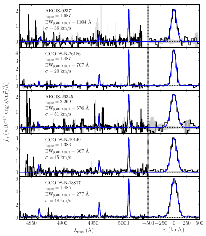
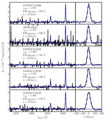
Figure 1: Example Keck/MOSFIRE spectra of ten EELGs at $z=1.3-2.4$ in our Sample I, in decreasing [O III] EW order. The left panel of each plot shows detections of H$\beta$, [O III] $\lambda 4959$, and [O III] $\lambda 5007$ emission lines. Blue curves present the best-fitting emission line profiles, and grey shaded regions present $\pm 1\sigma$ uncertainties. The right panel of each plot shows the zoom-in [O III] $\lambda 5007$ emission line profile (in velocity space), and the line width is used to compute the velocity dispersion. The resolution of our Keck/MOSFIRE spectra ranges from $R=3318$ to $R=3660$.

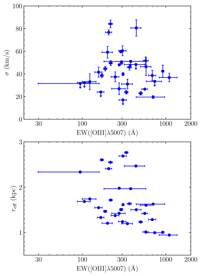
Figure 2: The velocity dispersion (measured from [O III] $\lambda 5007$ emission line width; top panel) and the effective radius (half-light radius; bottom panel) as functions of [O III] $\lambda 5007$ EW for our EELGs at $z=1.3-2.4$ with Keck/MOSFIRE spectra (Sample I). Objects with velocity dispersion smaller than the instrument resolution are shown as $3\sigma$ upper limits. Galaxies with the largest [O III] EWs tend to have smaller velocity dispersions, though with large scatter. Galaxies with larger [O III] EWs are also more compact sources with smaller sizes.

ID	R.A.	Decl.	$z_{\rm{spec}}$	EW[OIII]λ5007	$\log{(M_{\star,\rm{CSFH}}/M_{\odot})}$	sSFRCSFH	$\sigma$	$r_{\rm{eff}}$	$\log{(M_{\rm{dyn}}/M_{\odot})}$
	(hh:mm:ss)	(dd:mm:ss)		(Å)		(Gyr-1)	(km s-1)	(kpc)
COSMOS-19180	10:00:26.847	+02:22:26.727	$1.213$	$295\pm 10$	$8.74^{+0.05}_{-0.06}$	$13^{+2}_{-2}$	$50\pm 1$	$1.5$	$9.42\pm 0.38$
GOODS-S-28288	03:32:18.251	-27:46:51.964	$1.234$	$188\pm 8$	$9.02^{+0.05}_{-0.05}$	$3^{+0}_{-0}$	$44\pm 2$	$1.5$	$9.31\pm 0.38$
UDS-27523	02:17:06.812	-05:11:00.694	$1.670$	$123\pm 23$	$9.36^{+0.08}_{-0.06}$	$2^{+0}_{-0}$	$33\pm 7$	$1.7$	$9.12\pm 0.44$
UDS-36954	02:17:14.900	-05:09:06.174	$1.658$	$248\pm 27$	$9.12^{+0.08}_{-0.07}$	$6^{+2}_{-1}$	$37\pm 4$	$1.4$	$9.13\pm 0.40$
UDS-37070	02:17:04.624	-05:09:05.512	$1.416$	$94\pm 64$	$9.61^{+0.05}_{-0.06}$	$1^{+0}_{-0}$	$<31$	$2.3$	$<9.21$
AEGIS-02245	14:20:14.359	+52:54:09.481	$2.279$	$690\pm 70$	$8.19^{+0.20}_{-0.19}$	$38^{+21}_{-16}$	$38\pm 4$	$1.3$	$9.12\pm 0.40$
AEGIS-14784	14:20:08.796	+52:56:21.812	$2.291$	$218\pm 12$	$9.76^{+0.07}_{-0.06}$	$11^{+3}_{-2}$	$84\pm 3$	$2.5$	$10.10\pm 0.38$
AEGIS-15929	14:20:05.999	+52:56:10.029	$2.206$	$444\pm 62$	$8.67^{+0.12}_{-0.14}$	$33^{+24}_{-12}$	$80\pm 7$	$1.5$	$9.83\pm 0.39$
AEGIS-17167	14:19:55.518	+52:54:36.796	$2.207$	$157\pm 15$	$9.61^{+0.09}_{-0.15}$	$4^{+2}_{-1}$	$41\pm 4$	$1.5$	$9.27\pm 0.39$
AEGIS-29345	14:19:49.797	+52:56:30.463	$2.269$	$576\pm 41$	$8.15^{+0.22}_{-0.10}$	$70^{+16}_{-32}$	$51\pm 3$	$1.0$	$9.27\pm 0.38$
AEGIS-02371	14:20:47.930	+53:00:06.537	$1.687$	$1104\pm 268$	$7.18^{+0.17}_{-0.12}$	$151^{+57}_{-49}$	$36\pm 3$	$0.9$	$8.95\pm 0.39$
AEGIS-17916	14:20:25.737	+53:00:08.473	$1.628$	$307\pm 31$	$9.06^{+0.06}_{-0.08}$	$4^{+1}_{-0}$	$<17$	$2.7$	$<8.73$
AEGIS-10988	14:20:02.853	+52:54:26.496	$1.566$	$106\pm 19$	$8.91^{+0.19}_{-0.19}$	$1^{+1}_{-0}$	$<32$	$1.7$	$<9.09$
AEGIS-15240	14:19:56.598	+52:54:16.966	$1.648$	$171\pm 7$	$9.25^{+0.08}_{-0.09}$	$2^{+1}_{-0}$	$38\pm 1$	$2.6$	$9.43\pm 0.38$
AEGIS-15569	14:19:50.977	+52:53:25.728	$1.674$	$348\pm 52$	$8.40^{+0.17}_{-0.16}$	$8^{+6}_{-3}$	$31\pm 4$	$1.2$	$8.90\pm 0.40$
AEGIS-19374	14:19:57.008	+52:55:27.003	$1.685$	$380\pm 198$	$7.75^{+0.26}_{-0.29}$	$32^{+40}_{-17}$	$<51$	$2.0$	$<9.55$
AEGIS-22858	14:19:55.093	+52:55:55.815	$1.397$	$738\pm 154$	$7.56^{+0.21}_{-0.16}$	$79^{+40}_{-34}$	$<33$	$1.0$	$<8.89$
AEGIS-26531	14:19:52.778	+52:56:21.812	$1.588$	$303\pm 31$	$8.73^{+0.08}_{-0.08}$	$9^{+2}_{-2}$	$60\pm 4$	$1.2$	$9.50\pm 0.38$
AEGIS-29378	14:19:47.585	+52:56:07.873	$1.683$	$276\pm 51$	$8.55^{+0.11}_{-0.15}$	$5^{+2}_{-1}$	$26\pm 5$	$1.4$	$8.85\pm 0.43$
AEGIS-34848	14:19:39.730	+52:56:00.265	$1.524$	$200\pm 28$	$9.17^{+0.07}_{-0.08}$	$5^{+4}_{-2}$	$59\pm 5$	$1.2$	$9.47\pm 0.39$
GOODS-N-13876	12:36:10.789	+62:12:39.078	$1.625$	$581\pm 85$	$8.13^{+0.19}_{-0.25}$	$39^{+45}_{-16}$	$46\pm 7$	$1.6$	$9.38\pm 0.42$
GOODS-N-18360	12:36:10.480	+62:13:58.559	$1.674$	$923\pm 32$	$7.64^{+0.14}_{-0.12}$	$81^{+33}_{-23}$	$42\pm 5$	$1.0$	$9.10\pm 0.40$
GOODS-N-18548	12:36:17.755	+62:14:00.517	$1.485$	$337\pm 16$	$8.60^{+0.11}_{-0.15}$	$5^{+3}_{-1}$	$23\pm 1$	$2.8$	$9.04\pm 0.38$
GOODS-N-19659	12:36:24.654	+62:14:18.762	$1.451$	$289\pm 5$	$8.84^{+0.09}_{-0.06}$	$14^{+10}_{-4}$	$59\pm 1$	$1.5$	$9.57\pm 0.38$
GOODS-N-23634	12:36:27.007	+62:15:29.858	$1.676$	$440\pm 121$	$8.31^{+0.16}_{-0.14}$	$22^{+14}_{-9}$	$<48$	$2.5$	$<9.60$
GOODS-N-19149	12:36:32.669	+62:14:11.360	$1.383$	$367\pm 21$	$8.18^{+0.12}_{-0.11}$	$17^{+7}_{-4}$	$45\pm 2$	$1.6$	$9.38\pm 0.38$
GOODS-N-18817	12:36:40.516	+62:14:03.574	$1.485$	$277\pm 6$	$8.87^{+0.05}_{-0.05}$	$10^{+2}_{-1}$	$48\pm 1$	$2.0$	$9.50\pm 0.38$
GOODS-N-26186	12:36:38.417	+62:16:13.757	$1.487$	$707\pm 264$	$7.40^{+0.12}_{-0.08}$	$165^{+38}_{-42}$	$20\pm 1$	$1.6$	$8.64\pm 0.38$
GOODS-N-22263	12:37:17.724	+62:15:06.145	$1.488$	$501\pm 24$	$7.92^{+0.15}_{-0.16}$	$22^{+15}_{-8}$	$22\pm 1$	$1.2$	$8.65\pm 0.38$
GOODS-N-25465	12:37:21.196	+62:16:00.840	$1.433$	$166\pm 15$	$8.74^{+0.08}_{-0.09}$	$8^{+2}_{-2}$	$<24$	$1.3$	$<8.73$
GOODS-N-29675	12:37:07.081	+62:17:18.971	$1.684$	$561\pm 43$	$8.20^{+0.11}_{-0.12}$	$41^{+18}_{-10}$	$26\pm 0$	$1.4$	$8.84\pm 0.38$
GOODS-N-29190	12:36:56.424	+62:17:09.787	$1.488$	$219\pm 9$	$8.59^{+0.07}_{-0.08}$	$13^{+4}_{-3}$	$49\pm 2$	$1.7$	$9.47\pm 0.38$
GOODS-N-33726	12:36:59.343	+62:18:52.358	$1.450$	$308\pm 9$	$8.64^{+0.09}_{-0.08}$	$6^{+3}_{-2}$	$39\pm 1$	$1.6$	$9.25\pm 0.38$
GOODS-N-33438	12:36:43.891	+62:18:45.842	$1.684$	$207\pm 18$	$9.34^{+0.06}_{-0.07}$	$9^{+3}_{-2}$	$76\pm 2$	$2.4$	$9.99\pm 0.38$

Table 2: Coordinates, spectroscopic redshifts, [O III] $\lambda 5007$ EWs, stellar masses, sSFRs, velocity dispersions, effective radii, and dynamical masses of the $34$ EELGs in our Sample I. Redshifts are derived from [O III] $\lambda 5007$ emission lines. Stellar masses and sSFRs are derived from BEAGLE SED fitting with constant SFH models (Section 3.1). Velocity dispersions are computed from resolved [O III] $\lambda 5007$ emission line widths, and effective radii are measured from HST/WFC3 F160W imaging. Dynamical masses are computed using velocity dispersions and effective radii (Section 4.1).

ID	R.A.	Decl.	$z_{\rm{spec}}$	EW[OIII]λ5007	$\log{(M_{\star,\rm{CSFH}}/M_{\odot})}$	sSFRCSFH	ageCSFH
	(hh:mm:ss)	(dd:mm:ss)		(Å)		(Gyr-1)	(Myr)
AEGIS-04711	14:19:34.958	$+$52:47:50.219	$2.1839$	$1060\pm 25$	$2.3^{+0.1}_{-0.1}\times 10^{8}$	$118^{+9}_{-10}$	$8.5^{+0.8}_{-0.7}$
AEGIS-15778	14:19:11.210	$+$52:46:23.414	$2.1716$	$1001\pm 42$	$1.3^{+0.1}_{-0.1}\times 10^{8}$	$161^{+13}_{-13}$	$6.2^{+0.6}_{-0.5}$
UDS-08078	02:17:02.741	$-$05:14:57.498	$3.2277$	$881\pm 20$	$1.6^{+0.2}_{-0.1}\times 10^{9}$	$85^{+13}_{-14}$	$11.7^{+2.4}_{-1.5}$
UDS-09067	02:17:01.477	$-$05:14:45.359	$3.2288$	$1694\pm 42$	$3.0^{+0.3}_{-0.2}\times 10^{8}$	$136^{+12}_{-12}$	$7.3^{+0.8}_{-0.6}$
UDS-12539	02:17:53.733	$-$05:14:03.196	$1.6211$	$882\pm 33$	$1.1^{+0.1}_{-0.0}\times 10^{8}$	$188^{+8}_{-10}$	$5.3^{+0.3}_{-0.2}$
UDS-19167	02:17:43.535	$-$05:12:43.610	$2.1843$	$1532\pm 133$	$7.2^{+0.2}_{-0.2}\times 10^{7}$	$237^{+11}_{-11}$	$4.2^{+0.2}_{-0.2}$
UDS-21724	02:17:20.006	$-$05:12:10.624	$3.2278$	$1061\pm 34$	$3.3^{+0.3}_{-0.3}\times 10^{8}$	$137^{+9}_{-10}$	$7.3^{+0.7}_{-0.5}$

Table 3: Coordinates, spectroscopic redshifts, [O III] $\lambda 5007$ EWs, stellar masses, sSFRs, and stellar ages of the $7$ the most extreme [O III] emitters in our Sample II. The stellar masses, sSFRs, and stellar ages are derived from constant SFH models with BEAGLE (Section 3.1).

3 Spectral energy distribution fitting

We derive the physical properties (e.g., stellar mass) and constrain the stellar populations of EELGs in our Samples I and II from SED fitting. We first consider stellar population synthesis modeling with a constant star formation history using the BayEsian Analysis of GaLaxy sEds (BEAGLE, version 0.23.0; Chevallard & Charlot 2016) tool in Section 3.1. To better constrain potential older stellar populations ($>$ a few hundred Myr) in the most extreme [O III] emitters in Sample II, we also perform SED fitting with nonparametric SFH models using the Bayesian Analysis of Galaxies for Physical Inference and Parameter EStimation (BAGPIPES; Carnall et al. 2018) in Section 3.2.

3.1 Constant SFH model fitting

Following the procedures in T19, we model the broadband photometry and available emission line fluxes ([O II], H$\beta$, [O III], H$\alpha$) of the objects in Samples I and II using the BEAGLE tool. Here we use single stellar population models assuming a constant SFH (hereafter CSFH models). For the EELGs in Sample I, the stellar masses derived from CSFH model fitting are compared with dynamical masses in Section 4.1. We also examine whether the CSFH models are able to recover the rest-frame NIR luminosities of the most extreme [O III] emitters in Sample II, which may probe the hidden older stellar populations that might be masked by very young stars ($<10$ Myr) at rest-frame UV-to-optical wavelengths.

Details of the BEAGLE modeling have been described in T19 and we briefly summarise in the following. BEAGLE adopts the combination of the latest version of the Bruzual & Charlot (2003) stellar population synthesis models and the photoionisation models of star-forming galaxies of Gutkin et al. (2016) with CLOUDY (Ferland et al., 2013). We adopt a Chabrier (2003) initial mass function (IMF) and allow the metallicity to vary in the range $-2.2\leq\log{(Z/Z_{\odot})}\leq 0.25$ ($Z_{\odot}=0.01524$; Caffau et al. 2011). The gas-phase metallicity is set to equal to the stellar metallicity. The electron density is fixed to $n_{e}=100$ cm^-3 consistent with the density inferred from typical star-forming galaxies at $z\sim 2$ (e.g., Sanders et al., 2016; Steidel et al., 2016). The ionisation parameter $U$ and the dust-to-metal ratio $\xi_{\rm{d}}$ are adjusted in the range $-4.0\leq\log{U_{\rm{S}}}\leq-1.0$ and $0.1\leq\xi_{\rm{d}}\leq 0.5$. We assume the Calzetti et al. (2000) extinction curve to account for the dust attenuation in the neutral interstellar medium (ISM), and we adopt the prescription of Inoue et al. (2014) to include the absorption of intergalactic medium (IGM).

The best-fitting stellar masses and sSFRs are presented in Table 2. We find similar stellar mass and sSFR versus [O III] $\lambda 5007$ EW trends for Sample I as in T19, namely that galaxies with the largest [O III] $\lambda 5007$ EWs ($>800$ Å) have the lowest stellar masses ($M_{\star}\simeq 10^{7}-10^{8}\ M_{\odot}$) and undergo intense bursts of star formation (sSFR $\gtrsim 100$ Gyr^-1). For objects in Sample II, we fit the rest-frame UV-to-NIR SEDs with CSFH models as their robust IRAC (rest-frame NIR) fluxes are available, and the best-fitting stellar masses are presented in Table 3.

3.2 Nonparametric SFH model fitting

Nonparametric SFH fitting has the advantage it can recover more complex SFHs of galaxies (e.g., Tojeiro et al., 2007; Pacifici et al., 2016; Iyer et al., 2019; Leja et al., 2019; Lower et al., 2020; Tacchella et al., 2022a). In order to better reconstruct the potential past SFHs of the most extreme [O III] emitting galaxies, we use nonparametric SFH stellar population models to fit the rest-frame UV-to-NIR SEDs of the $7$ objects in Sample II using BAGPIPES. BAGPIPES uses the 2016 version of the Bruzual & Charlot (2003) stellar population synthesis models with a Kroupa (2001) IMF, and implements nebular emission models constructed using the CLOUDY photoionisation code following the methodology of Byler et al. (2017). We allow the metallicity to vary from $0$ to $2.5\ Z_{\odot}$. The ionisation parameter is fixed to $\log{U}=-2.0$, which is consistent with the typical ionisation parameter derived for the most extreme line emitters from BEAGLE (Tang et al., 2021a, b). We assume the Calzetti et al. (2000) extinction curve, with the dust attenuation ($A_{V}$) varies in the range $0-2$.

In order to recover the presence of earlier stellar populations, we fit the observed SEDs with nonparametric models for the mass formed in a series of piecewise constant functions in lookback time. With BAGPIPES we adopt the following seven time bins in models (where $t$ represents the lookback time):

$$0< t <3\ \rm{Myr};$$

$$3< t <10\ \rm{Myr};$$

$$10< t <30\ \rm{Myr};$$

$$30< t <100\ \rm{Myr};$$

$$100< t <300\ \rm{Myr};$$

$$300\ \rm{Myr}< t <1\ \rm{Gyr};$$

$$1\ \rm{Gyr}< t <4\ \rm{Gyr}.$$

Each time bin is spaced equally in logarithmic scale except the first and the last bin, as is common practice in the use of nonparametric SFH studies and it is more scalable in a sampling framework (e.g., Leja et al., 2017, 2019; Tacchella et al., 2022a). Such an approach is also consistent with Ocvirk et al. (2006) who find that the distinguish ability of simple stellar populations is roughly proportional to their separation in logarithmic time. For each time bin, we assume a constant SFH and fit the stellar mass formed in the bin as a free parameter (in the range $1<\log{(M_{\star}/M_{\odot})}<15$; the $\log{M}$ prior, see Leja et al. 2019). The BAGPIPES SED fitting is performed using Bayesian statistical techniques with nested sampling algorithms. The code outputs the posterior distribution of the stellar mass formed in each time bin and we compute the corresponding star formation rate. We will describe the stellar masses and stellar populations of the most extreme [O III] emitters in Sample II derived from both parametric and nonparametric model fitting in Section 4.2.

4 Constraining evolved stellar populations in the most extreme [O III] emitters

In this section, we address the possibility of evolved stellar populations in the most extreme [O III] emitting galaxies using dynamical mass measurements and SFHs derived from SED fitting. We first quantify the dependence of the dynamical mass and the dynamical-to-stellar mass ratio on [O III] EW for the objects in our Sample I (Section 4.1). We then characterize the stellar populations and SFHs of the most extreme [O III] emitting galaxies by fitting the rest-frame UV-to-NIR SEDs of the objects in Sample II (Section 4.2).

4.1 Dynamical masses of extreme [O III] emitters

The most intense optical line emitting galaxies have been found to have very young stellar ages ($<10$ Myr) and low stellar masses by fitting SEDs with constant SFH stellar population models (T19). If there are hidden older stellar populations in these systems, we would expect very large dynamical masses compared to the stellar masses inferred from CSFH models, and hence an increasing dynamical-to-stellar (CSFH) mass ratio with [O III] EW or sSFR (derived from CSFH models). The dynamical masses are computed using velocity dispersions measured from resolved [O III] $\lambda 5007$ emission line and half-light radii, and adopt the equation in Maseda et al. (2013):

$$M_{\rm{dyn}}=C\frac{r_{\rm{eff}}\sigma^{2}}{G},$$ (1)

where $\sigma$ is the velocity dispersion and $r_{\rm{eff}}$ is the half-light radius. The typical uncertainty of the half-light radius of EELGs at $z\sim 2$ is $10$ per cent (van der Wel et al., 2012; Maseda et al., 2014), and we adopt this in estimating the uncertainty of dynamical mass. The factor $C$ depends on the kinematic properties of galaxies. According to Price et al. (2016), dispersion-dominated galaxies result in $C\approx 5$, while $C\approx 2.7$ is adopted for rotation-dominated galaxies. Erb et al. (2006) assume a disk geometry and derive $C\approx 3.4$. In order to be consistent with other studies of emission line galaxies at $z\sim 1-2$ (e.g., Maseda et al., 2014; Masters et al., 2014), we adopt $C=3$ as used in Maseda et al. (2013) with a conservative uncertainty of $33$ per cent (e.g., Rix et al., 1997).

The dynamical masses of the EELGs in Sample I are presented in Table 2; they range from $10^{8.6}\ M_{\odot}$ to $10^{10.1}\ M_{\odot}$ with a median value of $10^{9.3}\ M_{\odot}$. These are systematically lower than the dynamical masses of typical $z\sim 2$ star-forming galaxies ($\sim 10^{10}-10^{11}\ M_{\odot}$; e.g., Erb et al. 2006; Price et al. 2016). In Fig. 3, we show the dynamical mass as functions of the [O III] $\lambda 5007$ EW and sSFR (derived from CSFH models) for our sample, and also the dynamical masses of the $22$ EELGs at $z\sim 1-2$ in Maseda et al. (2014). We notice that the Maseda et al. (2014) sample has slightly larger dynamical masses at fixed [O III] EW or sSFR compared to our sample as a result of their brighter targets. For both samples we find a moderate correlation between dynamical mass and [O III] EW (Spearman correlation coefficient $\rho=-0.45$ and $p$-value $p=1.9\times 10^{-2}$) and a weak correlation between dynamical mass and sSFR ($\rho=-0.18$, $p=0.37$), that galaxies with larger [O III] EWs or sSFRs have lower dynamical masses. For the most extreme line emitters with [O III] $\lambda 5007$ EW $>800$ Å or sSFR${}_{\rm{CSFH}}>100$ Gyr^-1, the dynamical masses (median $M_{\rm{dyn}}=10^{9.1}\ M_{\odot}$) are $\sim 2\times$ lower than those of galaxies with lower EWs (median $M_{\rm{dyn}}=10^{9.3}\ M_{\odot}$). This confirms the previous findings that the most extreme optical line emitting galaxies are low-mass systems (e.g., Reddy et al. 2018; T19; Sanders et al. 2020).

We next constrain the presence of older stellar populations in the most extreme [O III] emitters by comparing the dynamical mass to the stellar mass inferred from CSFH models. In Fig. 4, we plot the dynamical-to-stellar mass ratios of the objects in Sample I (blue solid circles) together with those of the Maseda et al. (2014) sample (grey open circles). In order to be consistent, we re-compute the stellar masses of the EELGs in Maseda et al. (2014) with BEAGLE, assuming single stellar population models with CSFH and following the same procedures as for our objects (see Section 3.1). It is remarkable that the dynamical-to-stellar mass ratio is strongly correlated with [O III] EW (Spearman correlation coefficient $\rho=0.84$ and $p$-value $p=3.5\times 10^{-8}$) and sSFR ($\rho=0.90$, $p=1.1\times 10^{-10}$), that the ratio increases with [O III] EW and sSFR_CSFH for both EELG samples. The median dynamical-to-stellar mass ratio of galaxies with [O III] $\lambda 5007$ EW $<300$ Å is $M_{\rm{dyn}}/M_{\star,\rm{CSFH}}=2$, and then this value increases to $10$ for galaxies with [O III] $\lambda 5007$ EW $=300-800$ Å and sSFR${}_{\rm{CSFH}}\simeq 10$ Gyr^-1 (i.e., the average [O III] EW and sSFR of typical $z\simeq 7-8$ star-forming galaxies; e.g., Labbé et al. 2013; Endsley et al. 2021). For galaxies with the largest [O III] $\lambda 5007$ EWs ($>800$ Å) and sSFRs ($>100$ Gyr^-1), the median dynamical-to-stellar mass ratio is $M_{\rm{dyn}}/M_{\star,\rm{CSFH}}\simeq 20$ with a maximum reaching $M_{\rm{dyn}}/M_{\star,\rm{CSFH}}\simeq 100$. Previous studies of more massive star-forming galaxies at $z\sim 2$ have also shown a positive correlation between the dynamical-to-stellar mass ratio and sSFR (e.g., Price et al., 2016) or H$\alpha$ EW (e.g., Erb et al., 2006). The increase of dynamical-to-stellar mass ratio with optical line EW and sSFR_CSFH indicates that the mass of recently formed stars ($<10$ Myr assuming CSFH) in the most intense line emitting galaxies comprises only $\sim 1-10$ per cent of the total dynamical mass. This suggests the dominant mass must arise from other components such as dark matter, gas, and perhaps the older stellar populations. We investigate each possibility in turn.

Regarding dark matter, recent studies (e.g., Wuyts et al., 2016; Price et al., 2020) have compared the baryonic mass (i.e., stellar mass and gas mass) to the dynamical mass for typical $z\sim 2$ star-forming galaxies. The results show that dark matter contributes only a small fraction ($\lesssim 10$ per cent) to the total dynamical mass. Assuming these results are representative for our sample, it suggests the bulk of the excess mass must be baryonic (i.e., gas or evolved stellar populations).

As our EELGs are undergoing intense bursts of star formation, it is likely that these systems have a large gas fraction. Ignoring for the moment a contribution from from evolved stars, we infer that the gas fraction must approach $\sim 80-90$ per cent of the dynamical mass (assuming a dark matter fraction of $10$ per cent). The commonly-used Kennicutt-Schmidt (KS) law (Kennicutt, 1998) is likely inapplicable here since starburst galaxies have higher star formation efficiencies (e.g., Bouché et al., 2007; Genzel et al., 2010; Wuyts et al., 2016). Using gas masses derived from CO or far-infrared emission, recent studies find that the gas fraction increases with sSFR (e.g., Dessauges-Zavadsky et al., 2015; Genzel et al., 2015; Schinnerer et al., 2016), reaching to $\sim 50-90$ per cent at sSFR $\sim 10$ Gyr^-1. This is lower or only marginally comparable to that required to explain our dynamical-to-stellar mass ratios in the absence of older stars. Maseda et al. (2014) also derive gas fractions for their sample of $z\sim 1-2$ EELGs based on the Jeans and Toomre instability criteria and quote values of $>67$ per cent. In summary, it is still unclear whether our large dynamical-to-stellar mass ratios can be explained solely due to gaseous reservoirs. In the next subsection, we will provide new constraints on the presence of older stars by fitting the rest-frame UV-to-NIR SEDs.

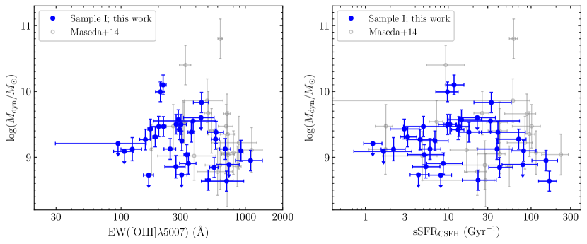
Figure 3: The dynamical mass versus [O III] $\lambda 5007$ EW (left panel) and sSFR (right panel) for the $34$ EELGs in our Sample I (blue solid circles) and the Maseda et al. (2014) EELGs at $z\sim 1-2$ (grey open circles). Objects with velocity dispersion smaller than instrument resolution are shown as $3\sigma$ upper limits. Galaxies with larger [O III] EWs or sSFRs tend to have lower dynamical masses, though with large scatter.

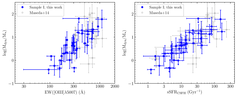
Figure 4: The dynamical-to-stellar mass ratio (assuming single stellar population models with CSFH) versus [O III] $\lambda 5007$ EW (left panel) and sSFR (inferred from single population CSFH models; right panel) for the $34$ EELGs in our Sample I (blue solid circles) and the Maseda et al. (2014) EELGs at $z\sim 1-2$ (grey open circles). A clear trend is shown that galaxies with larger [O III] EWs or sSFRs have larger dynamical-to-stellar mass ratios.

4.2 Stellar populations and star formation histories of the most extreme [O III] emitting galaxies

The final possibility for the large dynamical-to-stellar mass ratios is the presence of much older ($>$ a few hundred Myr) stars whose rest-frame UV-to-optical light is obscured by a young starburst. Such older stellar populations could be revealed via the SEDs of galaxies at rest-frame NIR wavelengths. In order to constrain the contribution of old stellar populations in the most extreme line emitters, we derive the stellar masses and SFHs of the $7$ galaxies with [O III] $\lambda 5007$ EW $>800$ Å and robust IRAC detections in our Sample II by fitting their rest-frame UV-to-NIR SEDs.

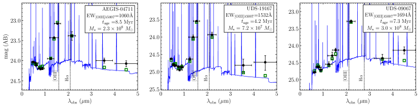
Figure 5: Broadband SEDs and the best-fitting CSFH models (derived from BEAGLE) of the most extreme [O III] emitters at $z=1.3-3.7$ with robust IRAC flux measurements in Sample II. Observed broadband photometry is shown as solid black circles. The best-fitting BEAGLE SED models are plotted by solid blue lines, and synthetic photometry is shown as open green squares. Strong rest-frame optical emission lines, [O III]$\lambda 5007$ and H$\alpha$, are highlighted by dashed black lines. Although the rest-frame UV-to-optical SEDs can be well reproduced by CSFH models, the rest-frame NIR (IRAC) luminosities for these objects are underestimated.

We first fit SEDs of the $7$ objects in Sample II using the constant CSFH models introduced in Section 3.1 with BEAGLE. The goal of this step is to investigate whether a single component stellar population model is able to reproduce the full observed SEDs especially at rest-frame NIR wavelengths. By fitting SEDs with CSFH models, we derive best-fitting stellar ages of the $7$ galaxies in Sample II ranging from $4$ to $12$ Myr. The stellar masses of these young systems are from $7\times 10^{7}\ M_{\odot}$ to $1.6\times 10^{9}\ M_{\odot}$ (Table 3). Although CSFH models can reproduce the rest-frame UV-to-optical SEDs of the most extreme line emitting sources, such models reproduce the observed IRAC (i.e., rest-frame NIR) luminosities for only $2$ of the $7$ objects in Sample II (UDS-08078, UDS-21724); they underestimate the IRAC luminosities for $5$ objects (AEGIS-04711, AEGIS-15778, UDS-09067, UDS-12539, UDS-19167). In Fig. 5, we plot rest-frame UV-to-NIR SEDs and the best-fitting CSFH models for the objects in Sample II. As shown in the figure, CSFH models only reproduce $50-80$ per cent of the observed IRAC luminosities, well below the observed $1\sigma$ lower limit.

We next fit SEDs of the objects in Sample II using nonparametric SFH models with BAGPIPES. As demonstrated in Section 3.2, we will derive the stellar masses formed in the seven lookback time bins from the most recent $3$ Myr to $>1$ Gyr ago. We aim to constrain the presence of possible older stellar populations in the most extreme optical line emitters, and whether the rest-frame NIR luminosities can be reproduced by including such stars. Note that in the following we will exclude UDS-21724 from our nonparametric SFH modeling since the strong nebular emission of this object cannot be well fitted by BAGPIPES which will result in an overestimation of the stellar mass.

The best-fitting BAGPIPES nonparametric SFH models for Sample II are plotted in Fig. 6. In contrast to the CSFH models, the SEDs and IRAC luminosities can be well reproduced within $1\sigma$ uncertainty by nonparametric SFH models. In Table 4 we present the stellar masses formed in the seven time bins for the objects in Sample II. We notice that the stellar masses formed in the first $10$ Myr inferred from nonparametric SFH models are from $5\times 10^{7}\ M_{\odot}$ to $5\times 10^{8}\ M_{\odot}$, roughly consistent with the stellar masses derived from CSFH models. More remarkably, however, a significant fraction of the total stellar mass was formed at $>100$ Myr ago. The evolved stellar masses of galaxies in Sample II range from $3\times 10^{9}\ M_{\odot}$ to $1\times 10^{10}\ M_{\odot}$, i.e. much greater than those associated with the secondary burst phase ($<10$ Myr). The results suggest that the rest-frame NIR light of these systems is likely dominated by stellar populations formed over a few hundred Myr ago, which cannot be easily identified at rest-frame UV-to-optical wavelengths.

The recovered SFHs from nonparametric models for objects in Sample II are also shown in Fig. 6. We notice that the models predict a “two-burst”-like SFH, the most recent $\leq 3$ Myr earlier following a first event between $100$ Myr and $1$ Gyr earlier. When EELGs are in the current burst phase, the massive stars are likely being formed in very young star clusters as demonstrated by spatially-resolved observations of a few strongly lensed galaxies at high redshift (e.g. Vanzella et al., 2019, 2022). When not in their present burst phase, they were forming stars with a negligible rate (lower than $10^{-2}\ M_{\odot}$ yr^-1 with large uncertainties). Such a low SFR implies a UV magnitude fainter than $31$ AB mag at $z\sim 2$, below the detection limit of current HST and even upcoming JWST imaging surveys (Robertson, 2021). However, we note that the recovered SFH does not necessarily mean these systems are actually in the quiescent phase between the two “bursts”. As reflected by the large uncertainties of SFRs (Fig. 6) and stellar masses (Table 4) formed between $\sim 10$ Myr and a few hundred Myr earlier, it is possible that the objects in Sample II followed a more gradual evolution during this period. The key point is that starlight from this period could be outshone by young massive stars at rest-frame UV-to-optical and by older stars at rest-frame NIR wavelengths. Nevertheless, we emphasise that the “burst” phase happened $>100$ Myr ago reflects the presence of evolved stellar populations in these systems.

Finally, we examine whether the extremely large dynamical-to-stellar mass ratios found in Section 4.1 could be explained by introducing evolved stellar populations inferred from nonparametric SFH fitting. Compared to the young stellar masses formed in the first $10$ Myr, the stellar masses formed at $>100$ Myr are $7-100\times$ (with a median of $39\times$) larger (Table 4), amounting to $87-99$ per cent (with a median of $97$ per cent) of the total stellar mass. This is consistent with studies of local extreme [O III] line emitting “Green Pea” galaxies (Cardamone et al., 2009) where only $\sim 4-20$ per cent of their stellar masses are produced in the most recent burst (Amorín et al., 2012). If the most intense line emitters in Sample II follow the $M_{\rm{dyn}}/M_{\star,\rm{CSFH}}$ - EW relation derived from our Sample I, the result could explain the large dynamical-to-stellar mass (derived from CSFH models) ratios ($M_{\rm{dyn}}/M_{\star,\rm{CSFH}}\simeq 10-100$) found for galaxies with [O III] $\lambda 5007$ EW $>800$ Å. The dynamical mass reflects not only the total stellar mass, but also the gas mass within the effective radius. Assuming the median old-to-young stellar mass ratio $\simeq 39$ derived from our Sample II, and the dynamical-to-stellar mass ratio $M_{\rm{dyn}}/M_{\star,\rm{CSFH}}\simeq 10-100$ found for the most extreme line emitters in Sample I, the gas fraction ($f_{\rm{gas}}=M_{\rm{gas}}/M_{\rm{dyn}}$) of the most extreme line emitters would be $60$ per cent or less. This is somewhat lower than the gas fraction derived for EELGs at $z\sim 1-2$ ($f_{\rm{gas}}\simeq 2/3$) in Maseda et al. (2014). On the other hand, if we assume the $f_{\rm{gas}}\simeq 2/3$ in Maseda et al. (2014), the evolved stellar mass needs to be $\simeq 3-33\times$ the young stellar mass in order to explain the dynamical-to-stellar mass ratio at EW${}_{\rm{[OIII]}}>800$ Å in Sample I, which is lower than the values derived in our Sample II. However, we consider this may be due to the following reasons. First, the current size of Sample II is small, and we focus on the subset with robust rest-frame NIR photometry detections which might bias the sample towards systems with larger evolved stellar mass (and hence brighter rest-frame NIR luminosity). Second, the gas fraction or the old-to-young stellar mass ratio may vary with [O III] EW, and the objects in our Sample II have larger [O III] EWs comparing to the average EW of the sample in Maseda et al. (2014). To test this scenario we need to compare with the gas fraction of the EW${}_{\rm{[OIII]}}>800$ Å galaxies in Maseda et al. (2014). However, there are only a handful (three) of such objects so currently the statistics are not good enough to make such comparison. Given the fact that the rest-frame UV-to-optical luminosities of the most intense optical line emitting galaxies are dominated by very young stellar populations, the SED fitting results demonstrate that the rest-frame NIR luminosity provides a valuable probe of the evolved stellar populations in these systems as reflected by their dynamical masses. In Section 5, we discuss the implications for the similar sources in the reionisation era.

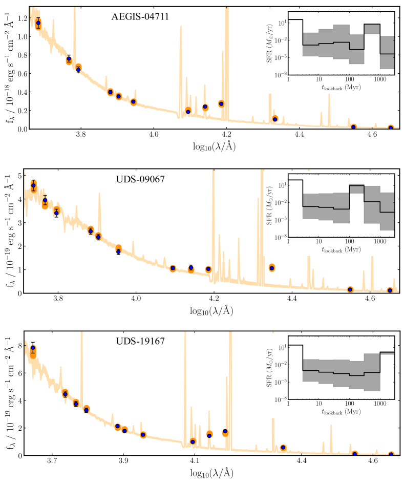
Figure 6: Broadband SEDs and the best-fitting nonparametric SFH models (derived from BAGPIPES) of the most extreme [O III] emitting galaxies in Sample II. Observed broadband fluxes including uncertainties are shown by blue circles, and the best-fitting model and the synthetic photometry (with the $84$th and $16$th percentiles) are shown by the orange line and the orange points. In the upper right of each SED plot, we show the SFH recovery of each object. The SFH is given by SFRs derived in the seven lookback time bins described in Section 3.2. Posterior median SFRs are plotted by black lines, and the grey shaded regions show the $16$th to $84$th percentiles (i.e., the $\pm 1\sigma$ uncertainties). The nonparametric SFH models can well reproduce the SEDs including the IRAC (rest-frame NIR) luminosities, and reconstruct the past SFHs ($>100$ Myr) for the most extreme [O III] emitters in addition to the intense bursts of star formation within $<10$ Myr.

Target ID	$\log{(M_{\star}/M_{\odot})}$	$\log{(M_{\star}/M_{\odot})}$	$\log{(M_{\star}/M_{\odot})}$	$\log{(M_{\star}/M_{\odot})}$	$\log{(M_{\star}/M_{\odot})}$	$\log{(M_{\star}/M_{\odot})}$	$\log{(M_{\star}/M_{\odot})}$
	$0-3$ Myr	$3-10$ Myr	$10-30$ Myr	$30-100$ Myr	$100-300$ Myr	$300$ Myr $-1$ Gyr	$>1$ Gyr
AEGIS-04711	$8.07^{+0.05}_{-0.05}$	$4.03^{+2.11}_{-1.92}$	$4.75^{+2.46}_{-2.31}$	$5.51^{+3.02}_{-2.88}$	$4.71^{+2.58}_{-2.47}$	$9.65^{+0.05}_{-1.68}$	$4.94^{+3.08}_{-2.58}$
AEGIS-15778	$7.67^{+0.16}_{-4.10}$	$6.17^{+1.79}_{-3.21}$	$4.30^{+2.32}_{-2.22}$	$4.59^{+2.38}_{-2.30}$	$4.92^{+3.06}_{-2.67}$	$9.67^{+0.05}_{-0.07}$	$5.34^{+2.66}_{-2.86}$
UDS-08078	$8.67^{+0.07}_{-2.94}$	$5.43^{+3.41}_{-2.95}$	$4.50^{+2.53}_{-2.34}$	$5.00^{+2.61}_{-2.64}$	$9.87^{+0.08}_{-4.57}$	$6.84^{+3.25}_{-3.85}$	$5.33^{+3.01}_{-2.82}$
UDS-09067	$8.41^{+0.05}_{-0.05}$	$4.17^{+2.20}_{-2.11}$	$4.49^{+2.39}_{-2.22}$	$4.73^{+2.79}_{-2.43}$	$9.25^{+0.27}_{-1.32}$	$7.01^{+2.68}_{-3.74}$	$5.65^{+3.37}_{-3.12}$
UDS-12539	$7.89^{+0.07}_{-0.12}$	$7.36^{+0.33}_{-0.46}$	$4.23^{+2.15}_{-1.98}$	$4.27^{+2.16}_{-2.13}$	$3.85^{+2.36}_{-1.81}$	$4.49^{+2.15}_{-2.06}$	$10.02^{+0.03}_{-0.03}$
UDS-19167	$7.89^{+0.04}_{-0.03}$	$3.85^{+1.92}_{-1.87}$	$4.03^{+2.11}_{-1.98}$	$4.33^{+2.37}_{-2.29}$	$4.44^{+2.47}_{-2.32}$	$5.52^{+3.25}_{-3.19}$	$9.49^{+0.11}_{-0.38}$

Table 4: Stellar masses formed in the seven lookback time bins for the most extreme [O III] emitting galaxies in Sample II. The time bins are introduced in Section 3.2, and the results are derived from BAGPIPES nonparametric SFH model fitting. A significant fraction of the total stellar mass is from evolved star formed at $>100$ Myr ago, and the mass of very young stellar populations ($<10$ Myr) compose a subdominant fraction of the total stellar mass.

5 Implications for stellar populations of galaxies in the reionisation era

The results described in Section 4 have suggested the possible presence of a significant population of evolved stars (age $>100$ Myr) in the most intense [O III] emitters at $z=1.3-3.7$. The evidence is based on both the extremely large dynamical masses compared to that derived for the young ($<10$ Myr) stellar population, and nonparametric SFHs recovered from fitting the rest-frame UV-to-NIR photometry. Although galaxies with EW${}_{\rm{[OIII]\lambda 5007}}>800$ Å are very rare at intermediate redshift (Boyett et al., 2021), this population is common in the reionisation era, comprising $20$ per cent at $z\sim 7$ (Endsley et al., 2021). Assuming our $z\sim 1-3$ EELG sample are representative of the sources at higher redshift, we consider the implications of our results for line emitting galaxies in the reionisation era.

Our results suggest that the stellar light associated with an evolved population would be masked by both the stellar and nebular emission at rest-frame UV and optical wavelengths from young starbursts. Upcoming JWST surveys with the Near Infrared Camera (NIRCam; Rieke et al. 2005) will target the rest-frame UV-to-optical imaging for a large population of galaxies at $z\gtrsim 7$, enabling more robust derivations of their stellar masses, SFRs and stellar ages (e.g. Tacchella et al., 2022b). Meanwhile, the analyses of our $z\simeq 1-3$ analogues suggest that the stellar masses and ages of the $z\simeq 7-8$ galaxies with the most extreme [O III] line emission may be significantly underestimated if they are based solely on analysing the rest-frame UV-to-optical photometry.

To illustrate this, we generate a mock galaxy spectrum at $z=8$ by adding a burst population (age $=5$ Myr) superposed on an evolved population with age $=300$ Myr following an instantaneous burst. Such a two-component system is consistent with a galaxy that first formed at $z\simeq 12$ and underwent a secondary burst phase of star formation at $z=8$. We use the latest Bruzual & Charlot (2003) stellar population synthesis models and incorporate nebular emission computed from the CLOUDY code. We assume a sub-solar metallicity ($Z=0.2Z_{\odot}$) and an ionisation parameter $\log{U}=-2$, consistent with recent estimates for sources in the reionisation era (e.g. Stark et al., 2017; Endsley et al., 2021). For various relative strengths of the burst and the evolved populations, we compute the JWST/NIRCam photometry for this mock $z=8$ galaxy using the NIRCam wide and medium filter transmission curves ensuring a SNR $=10$ to evaluate the uncertainties (i.e., the SNR that NIRCam reaches to observe a point source with M${}_{\rm{UV}}\simeq-18$ with $t\simeq 10$ ks; Robertson 2021). Using the BAGPIPES nonparametric SFH models described in Section 3.2, we attempt to detect the underlying evolved stellar population.

We find that even when the evolved stellar mass is $10\times$ the burst mass, nonparametric models cannot convincingly detect the presence of an evolved stellar population for the most extreme line emitters. This is the case for a system where we fix the burst ($5$ Myr) stellar mass to $10^{8}\ M_{\odot}$ and the evolved stellar mass to $10^{9}\ M_{\odot}$. Although the nonparametric models can adequately recover the mass formed in the burst phase ($M_{\star}=(1.1\pm 0.2)\times 10^{8}\ M_{\odot}$ in the $0-3$ Myr age bin), the stellar mass formed at $>100$ Myr is significantly underestimated (median $M_{\star}=1.8\times 10^{8}\ M_{\odot}$) with a large uncertainty ($1\sigma$ range $4\times 10^{3}-1\times 10^{9}\ M_{\odot}$). When the evolved stellar mass is $20\times$ the burst mass, it is more readily revealed (median $M_{\star}=1.5\times 10^{9}\ M_{\odot}$) but the uncertainty remains large ($1\sigma$ range $6\times 10^{3}-3\times 10^{9}\ M_{\odot}$). Here we notice that by choosing a different prior for the stellar mass distribution in the time bins in nonparametric SFH modeling (Section 3.2) might lead to a different median stellar mass. For example, a Dirichlet prior distribution favours an older mass-weighted stellar age or a longer star formation timescale (Leja et al., 2019; Tacchella et al., 2022a) than the uniform logarithm mass prior we used. Thus, we do not rule out that the choice of a different prior could potentially result in a derived median mass that was closer to the mass of the evolved population. However, without the knowledge of rest-frame NIR luminosity, it is difficult to robustly constrain the true stellar mass with small uncertainties.

The simulation described above reveals the large uncertainties associated with inferring the assembly history of galaxies in the reionisation era from such intense line emitters. Recent studies of $z\sim 7-8$ star-forming galaxies have argued that many are young systems with relatively low stellar masses (e.g. Labbé et al., 2013; Stefanon et al., 2022). These conclusions are usually derived by fitting the HST and Spitzer SEDs (i.e., rest-frame UV and optical at $z\sim 7-8$) with parametric SFH models (e.g., constant SFR). However, we have demonstrated in Section 4 that the stellar masses of EELGs could be underestimated by a factor of $\sim 40\times$ when considering CSFH fitting due to the difficulty of locating evolved stellar populations. Although it is perfectly possible that EELGs at $z\sim 1-3$ may not share the same SFHs as those at $z\sim 7-8$, our nonparametric fitting of mock NIRCam SEDs at $z=8$ suggests that the stellar masses of the most extreme line emitters could still be underestimated by $\sim 10\times$ if they are derived from rest-frame UV and optical photometry. Evidence of evolved stars has already been identified in a handful of galaxies at $z\gtrsim 9$ which formed prior to $z\simeq 12$ (e.g. Hashimoto et al., 2018; Roberts-Borsani et al., 2020; Laporte et al., 2021). As shown in the simulation at $z=8$ and the results inferred from EELGs at $z\sim 1-3$, if the stellar masses of the most extreme [O III] emitters (EW${}_{\rm{[OIII]}\lambda 5007}>800$ Å), which compose $20$ per cent of the $z\sim 7-8$ population (Endsley et al., 2021), were underestimated by a factor $\sim 10-40\times$, the total stellar mass density at $z\sim 7-8$ could be underestimated by a factor $\sim 2-8\times$. Conservatively, it seems reasonable to assume the mass density is underestimated by at least a factor $2\times$.

Finally, we consider the cosmic evolution of the UV luminosity density (and hence the SFR density) in the reionisation era in the context of the SFHs of EELGs presented in this study. Oesch et al. (2018) have argued for a rapid decline of the UV luminosity density at $z>8$, while McLeod et al. (2016) suggested a smoother decline. Here we revisit the test provided in the discussion sections of Roberts-Borsani et al. (2020) and Laporte et al. (2021). Considering the population of $z=8$ galaxies, we examine the fraction of their stellar mass that formed at earlier times. We focus on the stellar mass that formed at $z>9$, which represents an age $>100$ Myr for sources viewed at $z=8$. To derive the fraction of stellar mass formed at $z>9$ relative to $z=8$, we adopt the cosmic evolution of the SFR density in McLeod et al. (2016) and Oesch et al. (2018), which is converted from the UV luminosity density and assuming zero dust attenuation at $z>8$, and integrate the SFR with time to compute the stellar mass formed at a given redshift.

In Fig. 7, we show the redshift evolution of the fraction of stellar mass formed relative to $z=8$. Adopting the power-law function proposed by Oesch et al. (2014), a rapid decline of the UV luminosity density ($\rho_{\rm{UV}}\propto(1+z)^{-10.9}$) indicates that $27$ per cent of the stellar mass in $z=8$ galaxies was formed at $z>9$ (cyan dash-dotted line in Fig. 7), while this fraction becomes $58$ per cent in the case of smooth decline ($\rho_{\rm{UV}}\propto(1+z)^{-3.6}$; blue dashed line in Fig. 7). As demonstrated in our simulation of fitting NIRCam SEDs at $z=8$ with nonparametric SFH models, if the stellar masses of the most extreme line emitters (which compose $20$ per cent of the total population at $z=8$; Endsley et al. 2021) were underestimated by $10\times$, the total stellar mass density at $z=8$ could be underestimated by $2\times$. In this case, about $50$ per cent of the stellar mass at $z=8$ would be formed at $z>9$, which is consistent with a smooth decline of the UV luminosity density at $z>8$ (black solid line in Fig 7). Eventually, JWST observations with MIRI, which is capable of probing rest-frame NIR photometry at $z>7$, or deep NIRSpec observations targeting age indicators such as Balmer absorption lines, could help to determine the age and the assembly history of those systems in the reionisation era dominated by the light of very young stellar populations.

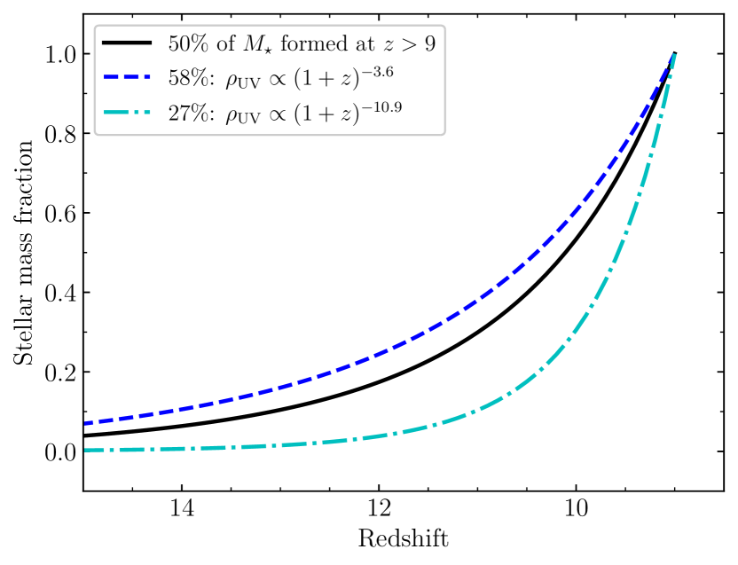
Figure 7: Redshift evolution of the fraction of stellar mass in $z=8$ galaxies that formed at $z>9$ (i.e., with an age $>100$ Myr). A smooth decline of UV luminosity function at $z>8$ ($\rho_{\rm{UV}}\propto[1+z]^{-3.6}$, blue dashed line; McLeod et al. 2016) would imply $58$ per cent of the stellar mass at $z=8$ was already in place at $z>9$, whereas this fraction would only be $27$ per cent in the case of a rapid decline ($\rho_{\rm{UV}}\propto[1+z]^{-10.9}$, cyan dash-dotted line; Oesch et al. 2018). As demonstrated in our simulation of fitting NIRCam SEDs at $z=8$ with nonparametric SFH models, the stellar masses of $20$ per cent of the galaxies at $z=8$ (i.e., the most extreme line emitters; Endsley et al. 2021) could be underestimated by $10\times$ if we only probe the rest-frame UV and optical photometry. Thus, the total stellar mass density at $z=8$ could be underestimated by $2\times$, that $50$ per cent of the stellar mass was formed at $z>9$ (black solid line, averaged at $z>9$), which favours a smooth decline. All the three curves are normalized at $z=9$.

Data Availability

The data underlying this article will be shared on reasonable request to the corresponding author.

References

- Amorín et al. (2012) Amorín R., Pérez-Montero E., Vílchez J. M., Papaderos P., 2012, ApJ, 749, 185
- Amorín et al. (2015) Amorín R., et al., 2015, A&A, 578, A105
- Astropy Collaboration et al. (2013) Astropy Collaboration et al., 2013, A&A, 558, A33
- Atek et al. (2011) Atek H., et al., 2011, ApJ, 743, 121
- Atek et al. (2014) Atek H., et al., 2014, ApJ, 789, 96
- Bertin & Arnouts (1996) Bertin E., Arnouts S., 1996, A&AS, 117, 393
- Bouché et al. (2007) Bouché N., et al., 2007, ApJ, 671, 303
- Boyett et al. (2021) Boyett K. N. K., Stark D. P., Bunker A. J., Tang M., Maseda M. V., 2021, arXiv e-prints, p. arXiv:2110.15858
- Brammer et al. (2012) Brammer G. B., et al., 2012, ApJS, 200, 13
- Bruzual & Charlot (2003) Bruzual G., Charlot S., 2003, MNRAS, 344, 1000
- Byler et al. (2017) Byler N., Dalcanton J. J., Conroy C., Johnson B. D., 2017, ApJ, 840, 44
- Caffau et al. (2011) Caffau E., Ludwig H. G., Steffen M., Freytag B., Bonifacio P., 2011, Sol. Phys., 268, 255
- Calzetti et al. (2000) Calzetti D., Armus L., Bohlin R. C., Kinney A. L., Koornneef J., Storchi-Bergmann T., 2000, ApJ, 533, 682
- Cardamone et al. (2009) Cardamone C., et al., 2009, MNRAS, 399, 1191
- Cardelli et al. (1989) Cardelli J. A., Clayton G. C., Mathis J. S., 1989, ApJ, 345, 245
- Carnall et al. (2018) Carnall A. C., McLure R. J., Dunlop J. S., Davé R., 2018, MNRAS, 480, 4379
- Chabrier (2003) Chabrier G., 2003, PASP, 115, 763
- Chevallard & Charlot (2016) Chevallard J., Charlot S., 2016, MNRAS, 462, 1415
- Chilingarian et al. (2015) Chilingarian I., Beletsky Y., Moran S., Brown W., McLeod B., Fabricant D., 2015, PASP, 127, 406
- Coil et al. (2015) Coil A. L., et al., 2015, ApJ, 801, 35
- Dessauges-Zavadsky et al. (2015) Dessauges-Zavadsky M., et al., 2015, A&A, 577, A50
- Donley et al. (2012) Donley J. L., et al., 2012, ApJ, 748, 142
- Ellis et al. (2013) Ellis R. S., et al., 2013, ApJ, 763, L7
- Endsley et al. (2021) Endsley R., Stark D. P., Chevallard J., Charlot S., 2021, MNRAS, 500, 5229
- Erb et al. (2006) Erb D. K., Steidel C. C., Shapley A. E., Pettini M., Reddy N. A., Adelberger K. L., 2006, ApJ, 646, 107
- Ferland et al. (2013) Ferland G. J., et al., 2013, Rev. Mex. Astron. Astrofis., 49, 137
- Förster Schreiber et al. (2014) Förster Schreiber N. M., et al., 2014, ApJ, 787, 38
- Freeman et al. (2019) Freeman W. R., et al., 2019, ApJ, 873, 102
- Genzel et al. (2010) Genzel R., et al., 2010, MNRAS, 407, 2091
- Genzel et al. (2015) Genzel R., et al., 2015, ApJ, 800, 20
- Grogin et al. (2011) Grogin N. A., et al., 2011, ApJS, 197, 35
- Gutkin et al. (2016) Gutkin J., Charlot S., Bruzual G., 2016, MNRAS, 462, 1757
- Hashimoto et al. (2018) Hashimoto T., et al., 2018, Nature, 557, 392
- Hunter (2007) Hunter J. D., 2007, Computing in Science and Engineering, 9, 90
- Inoue et al. (2014) Inoue A. K., Shimizu I., Iwata I., Tanaka M., 2014, MNRAS, 442, 1805
- Iyer et al. (2019) Iyer K. G., Gawiser E., Faber S. M., Ferguson H. C., Kartaltepe J., Koekemoer A. M., Pacifici C., Somerville R. S., 2019, ApJ, 879, 116
- Jiang et al. (2021) Jiang L., et al., 2021, Nature Astronomy, 5, 256
- Jones et al. (2001) Jones E., Oliphant T., Peterson P., et al., 2001, SciPy: Open source scientific tools for Python, http://www.scipy.org/
- Kennicutt (1998) Kennicutt Robert C. J., 1998, ARA&A, 36, 189
- Koekemoer et al. (2011) Koekemoer A. M., et al., 2011, ApJS, 197, 36
- Kriek et al. (2015) Kriek M., et al., 2015, ApJS, 218, 15
- Kroupa (2001) Kroupa P., 2001, MNRAS, 322, 231
- Labbé et al. (2013) Labbé I., et al., 2013, ApJ, 777, L19
- Laporte et al. (2021) Laporte N., Meyer R. A., Ellis R. S., Robertson B. E., Chisholm J., Roberts-Borsani G. W., 2021, MNRAS, 505, 3336
- Leja et al. (2017) Leja J., Johnson B. D., Conroy C., van Dokkum P. G., Byler N., 2017, ApJ, 837, 170
- Leja et al. (2019) Leja J., Carnall A. C., Johnson B. D., Conroy C., Speagle J. S., 2019, ApJ, 876, 3
- Lower et al. (2020) Lower S., Narayanan D., Leja J., Johnson B. D., Conroy C., Davé R., 2020, ApJ, 904, 33
- Maseda et al. (2013) Maseda M. V., et al., 2013, ApJ, 778, L22
- Maseda et al. (2014) Maseda M. V., et al., 2014, ApJ, 791, 17
- Masters et al. (2014) Masters D., et al., 2014, ApJ, 785, 153
- McLean et al. (2010) McLean I. S., et al., 2010, in McLean I. S., Ramsay S. K., Takami H., eds, Society of Photo-Optical Instrumentation Engineers (SPIE) Conference Series Vol. 7735, Ground-based and Airborne Instrumentation for Astronomy III. p. 77351E, doi:10.1117/12.856715
- McLean et al. (2012) McLean I. S., et al., 2012, in McLean I. S., Ramsay S. K., Takami H., eds, Society of Photo-Optical Instrumentation Engineers (SPIE) Conference Series Vol. 8446, Ground-based and Airborne Instrumentation for Astronomy IV. p. 84460J, doi:10.1117/12.924794
- McLeod et al. (2012) McLeod B., et al., 2012, PASP, 124, 1318
- McLeod et al. (2016) McLeod D. J., McLure R. J., Dunlop J. S., 2016, MNRAS, 459, 3812
- Momcheva et al. (2016) Momcheva I. G., et al., 2016, ApJS, 225, 27
- Newman et al. (2012) Newman S. F., et al., 2012, ApJ, 761, 43
- Ocvirk et al. (2006) Ocvirk P., Pichon C., Lançon A., Thiébaut E., 2006, MNRAS, 365, 46
- Oesch et al. (2014) Oesch P. A., et al., 2014, ApJ, 786, 108
- Oesch et al. (2016) Oesch P. A., et al., 2016, ApJ, 819, 129
- Oesch et al. (2018) Oesch P. A., Bouwens R. J., Illingworth G. D., Labbé I., Stefanon M., 2018, ApJ, 855, 105
- Oke & Gunn (1983) Oke J. B., Gunn J. E., 1983, ApJ, 266, 713
- Osterbrock & Ferland (2006) Osterbrock D. E., Ferland G. J., 2006, Astrophysics of gaseous nebulae and active galactic nuclei
- Pacifici et al. (2016) Pacifici C., Oh S., Oh K., Lee J., Yi S. K., 2016, ApJ, 824, 45
- Planck Collaboration et al. (2020) Planck Collaboration et al., 2020, A&A, 641, A6
- Price et al. (2016) Price S. H., et al., 2016, ApJ, 819, 80
- Price et al. (2020) Price S. H., et al., 2020, ApJ, 894, 91
- Reddy et al. (2018) Reddy N. A., et al., 2018, ApJ, 853, 56
- Rieke et al. (2005) Rieke M. J., Kelly D., Horner S., 2005, in Heaney J. B., Burriesci L. G., eds, Society of Photo-Optical Instrumentation Engineers (SPIE) Conference Series Vol. 5904, Cryogenic Optical Systems and Instruments XI. pp 1–8, doi:10.1117/12.615554
- Rix et al. (1997) Rix H.-W., Guhathakurta P., Colless M., Ing K., 1997, MNRAS, 285, 779
- Roberts-Borsani et al. (2016) Roberts-Borsani G. W., et al., 2016, ApJ, 823, 143
- Roberts-Borsani et al. (2020) Roberts-Borsani G. W., Ellis R. S., Laporte N., 2020, MNRAS, 497, 3440
- Robertson (2021) Robertson B. E., 2021, arXiv e-prints, p. arXiv:2110.13160
- Robertson et al. (2015) Robertson B. E., Ellis R. S., Furlanetto S. R., Dunlop J. S., 2015, ApJ, 802, L19
- Salmon et al. (2018) Salmon B., et al., 2018, ApJ, 864, L22
- Sanders et al. (2016) Sanders R. L., et al., 2016, ApJ, 816, 23
- Sanders et al. (2020) Sanders R. L., et al., 2020, MNRAS, 491, 1427
- Schinnerer et al. (2016) Schinnerer E., et al., 2016, ApJ, 833, 112
- Skelton et al. (2014) Skelton R. E., et al., 2014, ApJS, 214, 24
- Smit et al. (2014) Smit R., et al., 2014, ApJ, 784, 58
- Smit et al. (2015) Smit R., et al., 2015, ApJ, 801, 122
- Stark et al. (2017) Stark D. P., et al., 2017, MNRAS, 464, 469
- Stefanon et al. (2022) Stefanon M., Bouwens R. J., Labbé I., Illingworth G. D., Oesch P. A., van Dokkum P., Gonzalez V., 2022, ApJ, 927, 48
- Steidel et al. (2016) Steidel C. C., Strom A. L., Pettini M., Rudie G. C., Reddy N. A., Trainor R. F., 2016, ApJ, 826, 159
- Tacchella et al. (2022a) Tacchella S., et al., 2022a, ApJ, 926, 134
- Tacchella et al. (2022b) Tacchella S., et al., 2022b, ApJ, 927, 170
- Tang et al. (2019) Tang M., Stark D. P., Chevallard J., Charlot S., 2019, MNRAS, 489, 2572
- Tang et al. (2021a) Tang M., Stark D. P., Chevallard J., Charlot S., Endsley R., Congiu E., 2021a, MNRAS, 501, 3238
- Tang et al. (2021b) Tang M., Stark D. P., Chevallard J., Charlot S., Endsley R., Congiu E., 2021b, MNRAS, 503, 4105
- Tojeiro et al. (2007) Tojeiro R., Heavens A. F., Jimenez R., Panter B., 2007, MNRAS, 381, 1252
- Vanzella et al. (2019) Vanzella E., et al., 2019, MNRAS, 483, 3618
- Vanzella et al. (2022) Vanzella E., et al., 2022, A&A, 659, A2
- Wuyts et al. (2016) Wuyts S., et al., 2016, ApJ, 831, 149
- van der Wel et al. (2011) van der Wel A., et al., 2011, ApJ, 742, 111
- van der Wel et al. (2012) van der Wel A., et al., 2012, ApJS, 203, 24