Abstract

Deep neural networks (DNNs) are currently predominantly trained using first-order methods. Some of these methods (e.g., Adam, AdaGrad, and RMSprop, and their variants) incorporate a small amount of curvature information by using a diagonal matrix to precondition the stochastic gradient. Recently, effective second-order methods, such as KFAC, K-BFGS, Shampoo, and TNT, have been developed for training DNNs, by preconditioning the stochastic gradient by layer-wise block-diagonal matrices. Here we propose a "mini-block Fisher (MBF)" "preconditioned gradient method, that lies in between these two classes of methods. Specifically, our method uses a block-diagonal approximation to the empirical Fisher matrix, where for each layer in the DNN, whether it is convolutional or feed-forward and fully connected, the associated diagonal block is itself block-diagonal and is composed of a large number of mini-blocks of modest size. Our novel approach utilizes the parallelism of GPUs to efficiently perform computations on the large number of matrices in each layer. Consequently, MBF’s per-iteration computational cost is only slightly higher than it is for first-order methods. The performance of our proposed method is compared to that of several baseline methods, on both autoencoder and CNN problems, to validate its effectiveness both in terms of time efficiency and generalization power. Finally, it is proved that an idealized version of MBF converges linearly.

1 Introduction

First-order methods based on stochastic gradient descent (SGD) (Robbins & Monro, 1951), and in particular, the class of adaptive learning rate methods, such as AdaGrad (Duchi et al., 2011), RMSprop (Hinton et al., 2012), and Adam (Kingma & Ba, 2014), are currently the most widely used methods to train deep learning models (the recent paper (Schmidt et al., 2021) lists 65 methods that have “Adam” or “Ada” as part of their names). While these methods are easy to implement and have low computational complexity, they make use of only a limited amount of curvature information. Standard SGD and its mini-batch variants, use none. SGD with momentum (SGD-m) (Polyak, 1964) and stochastic versions of Nesterov’s accelerated gradient method (Nesterov, 1998), implicitly make use of curvature by choosing step directions that combine the negative gradient with a scaled multiple of the previous step direction, very much like the classical conjugate gradient method.

To effectively optimize ill-conditioned functions, one usually needs to use second-order methods, which range from the Newton’s method to those that use approximations to the Hessian matrix, such as BFGS quasi-Newton (QN) methods (Broyden, 1970; Fletcher, 1970; Goldfarb, 1970; Shanno, 1970), including limited memory variants (Liu & Nocedal, 1989), and Gauss-Newton (GN) methods (Ortega & Rheinboldt, 1970). To handle large machine learning data sets, stochastic methods such as sub-sampled Newton (Xu et al., 2019)), QN (Byrd et al., 2016; Gower et al., 2016; Wang et al., 2017), GN, natural gradient (NG) (Amari et al., 2000), Hessian-free (Martens, 2010), and Krylov subspace methods (Vinyals & Povey, 2012) have been developed. However, in all of these methods, whether they use the Hessian or an approximation to it, the size of the matrix becomes prohibitive when the number of training parameters is huge.

Therefore, deep learning training methods have been proposed that use layer-wise block-diagonal approximations to the second-order preconditioning matrix. These include a Sherman-Morrison-Woodbury based variant (Ren & Goldfarb, 2019) and a low-rank variant (Roux et al., 2008) of the block-diagonal Fisher matrix approximations for NG methods. Also, Kronecker-factored matrix approximations of the diagonal blocks in Fisher matrices have been proposed to reduce the memory and computational requirements of NG methods, starting from KFAC for multilayer preceptrons (MLPs) (Martens & Grosse, 2015), which was extended to CNNs in (Grosse & Martens, 2016); (in addition, see Heskes (2000); Povey et al. (2014); George et al. (2018)). Kronecker-factored QN methods (Goldfarb et al., 2020), generalized GN methods (Botev et al., 2017), an adaptive block learning rate method Shampoo (Gupta et al., 2018) based on AdaGrad, and an approximate NG method TNT (Ren & Goldfarb, 2021b), based on the assumption that the sampled tensor gradient follows a tensor-normal distribution have also been proposed.

Our Contributions:

We propose here a new Mini-Block Fisher (MBF) gradient method that lies in between adaptive first-order methods and block diagonal second-order methods. Specifically, MBF uses a block-diagonal approximation to the empirical Fisher matrix, where for each DNN layer, whether it is convolutional or feed-forward and fully-connected, the associated diagonal block is also block-diagonal and is composed of a large number of mini-blocks of modest size.

Crucially, MBF has comparable memory requirements to those of first-order methods, while its per-iteration time complexity is smaller, and in many cases, much smaller than that of popular second-order methods (e.g. KFAC) for training DNNs. Further, we prove convergence results for a variant of MBF under relatively mild conditions.

In numerical experiments on well-established Autoencoder and CNN models, MBF consistently outperformed state-of-the-art (SOTA) first-order methods (SGD-m and Adam) and performed favorably compared to popular second-order methods (KFAC and Shampoo).

2 Notation and Definitions

Notation. $\text{Diag}_{i\in[L]}(A_{i})$ is the block diagonal matrix with $\{A_{1},...,A_{L}\}$ on its diagonal; $[L]:=\{1,...,L\}$; $\bm{X}=[x_{1},...,x_{n}]^{\top}\in\mathbb{R}^{n\times d}$ is the input data; $\lambda_{\min}(M),\lambda_{\max}(M)$ are the smallest and largest eigenvalues of the matrix $M$; $\otimes$ denotes the Kronecker product; $\|.\|_{2}$ denotes the Euclidean norm of a vector or matrix; and $\text{vec}(A)$ vectorizes $A$ by stacking its columns.

We consider a DNN with $L$ layers, defined by weight matrices ${W_{l}}$, for $l\in[L]$, that transforms the input vector $\bm{x}$ to an output $f(\bm{W},\bm{x})$. For a data-point $(x,y)$, the loss $\ell\left(f(\bm{W},\bm{x}),y\right)$ between the output $f(\bm{W},\bm{x})$ and $y$, is a non-convex function of $\operatorname{vec}(\bm{W})^{\top}=\left[\operatorname{vec}\left(W_{1}\right)^{\top},...,\operatorname{vec}\left(W_{L}\right)^{\top}\right]\in\mathbb{R}^{p}$, containing all of the network’s parameters, and $\ell$ measures the accuracy of the prediction (e.g. squared error loss, cross entropy loss). The optimal parameters are obtained by minimizing the average loss $\pazocal{L}$ over the training set:

$${\pazocal{L}(\bm{W})=\frac{1}{n}\sum_{i=1}^{n}\ell(f(\bm{W},\textbf{x}_{i}),\textbf{y}_{i}),}$$ (1)

This setting is applicable to most common models in deep learning such as multilayer perceptrons (MLPs), CNNs, recurrent neural networks (RNNs), etc. In these models, the trainable parameter $W_{l}$ ($l=1,\ldots,L$) come from the weights of a layer, whether it be a feed-forward, convolutional, recurrent, etc. For the weight matrix $W_{l}\in\mathbb{R}^{p_{l}}$ corresponding to layer $l$ and a subset of indices $b\subset\{1,\ldots,p_{l}\}$, we denote by $W_{l,b}$, the subset of parameters of $W_{l}$ corresponding to $b$.

The average gradient over a mini-batch of size $m$, $\bm{g}^{(m)}=\frac{1}{m}\sum_{i=1}^{m}\frac{\partial\ell(f(\bm{W},\textbf{x}_{i}),\textbf{y}_{i})}{\partial\bm{W}}$, is computed using standard back-propagation. In the full-batch case, where $m=n$, $\bm{g}^{(n)}=\bm{g}=\frac{\partial\pazocal{L}(\bm{W})}{\partial\bm{W}}=\mathcal{D}\bm{W}$. Here, we are using the notation $\mathcal{D}\bm{X}:=\frac{\partial\pazocal{L}(\bm{W})}{\partial\bm{X}}$ for any subset of variables $\bm{X}\subset\bm{W}$.

The Jacobian $\bm{J}(\bm{W})$ of the loss $\pazocal{L}(\cdot)$ w.r.t the parameters $\bm{W}$ for a single output network is defined as $\bm{J}=[\bm{J}_{1}^{\top},...,\bm{J}_{n}^{\top}]^{\top}\in\mathbb{R}^{n\times p}$, where $\bm{J}_{i}^{\top}$ is the gradient of the loss w.r.t the parameters, i.e., $\bm{J}_{i}^{\top}=\operatorname{vec}(\frac{\partial\ell(f(\bm{W},\textbf{x}_{i}),\textbf{y}_{i})}{\partial\bm{W}})$. We use the notation ${\bm{J}_{i}^{X}}^{\top}=\operatorname{vec}(\frac{\partial\ell(f(\bm{W},\textbf{x}_{i}),\textbf{y}_{i})}{\partial X})$ and $\bm{J}^{X}=[{\bm{J}_{1}^{X}}^{\top},...,{\bm{J}_{n}^{X}}^{\top}]^{\top}$ for any subset of variables $X$ of $\bm{W}$.

The Fisher matrix $\bm{F}(\bm{W})$ of the model’s conditional distribution is defined as

$$\bm{F}(\bm{W})=\underset{{\begin{subarray}{c}x\sim Q_{x}\\ y\sim p_{\bm{W}}(\cdot|x)\end{subarray}}}{\mathbb{E}}\left[\frac{\partial\log p_{\bm{W}}(y|x)}{\partial\bm{W}}\left(\frac{\partial\log p_{\bm{W}}(y|x)}{\partial\bm{W}}\right)^{\top}\right],$$

where $Q_{x}$ is the data distribution of $x$ and $p_{\bm{W}}(\cdot|x)$ is the density function of the conditional distribution defined by the model with a given input $x$. As shown in (Martens, 2020), $\bm{F}(\bm{W})$ is equivalent to the Generalized Gauss-Newton (GGN) matrix if the conditional distribution is in the exponential family, e.g., a categorical distribution for classification or a Gaussian distribution for regression.

The empirical Fisher matrix (EFM) $\tilde{\bm{F}}(\bm{W})$ defined as:

$$\tilde{\bm{F}}(\bm{W}) ={\frac{1}{n}\sum_{i=1}^{n}\frac{\partial\ell(f(\bm{W},\textbf{x}_{i}),\textbf{y}_{i})}{\partial\bm{W}}\frac{\partial\ell(f(\bm{W},\textbf{x}_{i}),\textbf{y}_{i})}{\partial\bm{W}}^{\top}}$$

$$=\frac{1}{n}\bm{J}(\bm{W})^{\top}\bm{J}(\bm{W}),$$

is obtained by replacing the expectation over the model’s distribution in $\bm{F}(\bm{W})$ by an average over the empirical data. MBF uses the EMF rather than the Fisher matrix, since doing so does not require extra backward passes to compute additional gradients and memory to store them. We note that, as discussed in (Kunstner et al., 2019) and (Thomas et al., 2020), the EMF, which is an un-centered second moment of the gradient, captures less curvature information than the Fisher matrix, which coincides with the GGN matrix in many important cases, and hence is closely related to $\nabla^{2}\pazocal{L}(\bm{W})$. To simplify notation we will henceforth drop the "tilde" $\tilde{}$ and denote the EFM by $\bm{F}$. We denote by $\bm{F}^{X}=\frac{1}{n}(\bm{J}^{X})^{\top}\bm{J}^{X}$, the sub-block of $\bm{F}(\bm{W})$ associated with any subset of variables $X\subset\bm{W}$, and write $(\bm{F}^{X})^{-1}$ as $F^{-1}_{X}$.

3 Mini-block Fisher (MBF) method

At each iteration, MBF preconditions the gradient direction by the inverse of a damped EFM:

$${\bm{W}(k+1)=\bm{W}(k)-\alpha\left(\bm{F}(\bm{W}(k))+\lambda\bm{I}\right)^{-1}\bm{g}(k),}$$ (2)

where $\alpha$ is the learning rate and $\lambda$ is the damping parameter.

To avoid the work of computing and storing the inverse of the $p\times p$ damped EFM, $(\bm{F}+\lambda I)^{-1}$, where $p$ can be in the millions, we assume, as in KFAC and Shampoo, that the EFM has a block diagonal structure, where the $l_{th}$ diagonal block corresponds to the second moment of the gradient of the model w.r.t to the weights in the $l_{th}$ layer. Hence, the block-diagonal EFM is:

$$\bm{F}(\bm{W})\approx\text{Diag}\left(\bm{F}^{W_{1}},...,\bm{F}^{W_{L}}\right).$$

Figure 1 summarizes how several existing methods further approximate these diagonal blocks.

Figure 1: MBF vs other block-diagonal preconditioned gradient methods

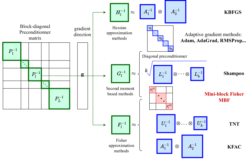
MBF further approximates each of the diagonal blocks $F_{W_{l}}$ by a block-diagonal matrix, composed of a typically large number mini-blocks, depending on the nature of layer $l$, as follows:

Figure 2: Illustration of MBF’s approximation for a convolutional layer.

Figure 3: Illustration of MBF’s preconditionner for a feed-forward fully-connected layer.

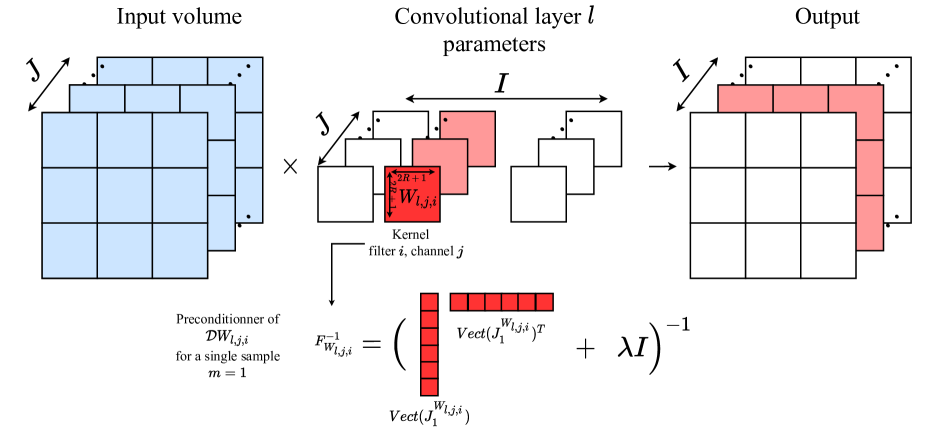
Layer $l$ is convolutionnal: For simplicity, we assume that the convolutional layer $l$ is 2-dimensional and has $J$ input channels indexed by $j=1,...,J$, and $I$ output channels indexed by $i=1,...,I$; there are $I\times O$ kernels $W_{l,j,i}$, each of size $(2R+1)\times(2R+1)$, with spatial offsets from the centers of each filter indexed by $\delta\in{\Delta}:=\{-R,...,R\}\times\{-R,...,R\}$; the stride is of length 1, and the padding is equal to $R$, so that the sets of input and output spatial locations ($t\in\mathcal{T}\subset\mathbf{R}^{2}$) are the same.. For such layers, we use the following $(IJ+1)\times(IJ+1)$ block-diagonal approximation to the $l_{th}$ diagonal block $\bm{F}^{W_{l}}$ of the Fisher matrix

$$\text{diag}\{\bm{F}^{W_{l,1,1}},...,\bm{F}^{W_{l,1,I}},...,\bm{F}^{W_{l,J,1}},...,\bm{F}^{W_{l,J,I}},\bm{F}^{b_{l}}\},$$

where each of the $IJ$ diagonal blocks $\bm{F}^{W_{l,j,i}}$ is a $|\Delta|\times|\Delta|$ symmetric matrix corresponding to the kernel vector $W_{l,j,i}$ and where $\bm{F}^{b_{l}}$ is an $I\times I$ diagonal matrix corresponding the bias vector $b_{l}$. Therefore, the preconditioning matrix $F^{-1}_{W_{l,j,i}}$ corresponding to the kernel for input-output channel pair $(j,i)$ is given by:

$$F^{-1}_{W_{l,j,i}}:=\left(\frac{1}{n}(\bm{J}^{W_{l,j,i}})^{T}\bm{J}^{W_{l,j,i}}+\lambda I\right)^{-1}$$

A common choice in CNNs is to use either a $3\times 3$ or $5\times 5$ kernel for all of the $IJ$ channel pairs in a layer. Therefore, all of these matrices are of the same (small) size, $|\Delta|\times|\Delta|$, and can be inverted efficiently by utilizing the parallelism of GPUs. We illustrate MBF’s approximation for a convolutional layer for the case of one data-point in Fig. 2. From Fig. 2, it is apparent that kernal matrices in a convolutional layer that connect input to output channels are analagous to scalar weights that connect input to output nodes in a ff-cc layer. Hence, MBF is analaous to using the squares of the components of the gradient in a ff-cc network, and hence is analagous to a "squared" version of an adaptive first-order method. This observation (detailed in Appendix 10) was in fact the motivation for our development of the MBF approach.

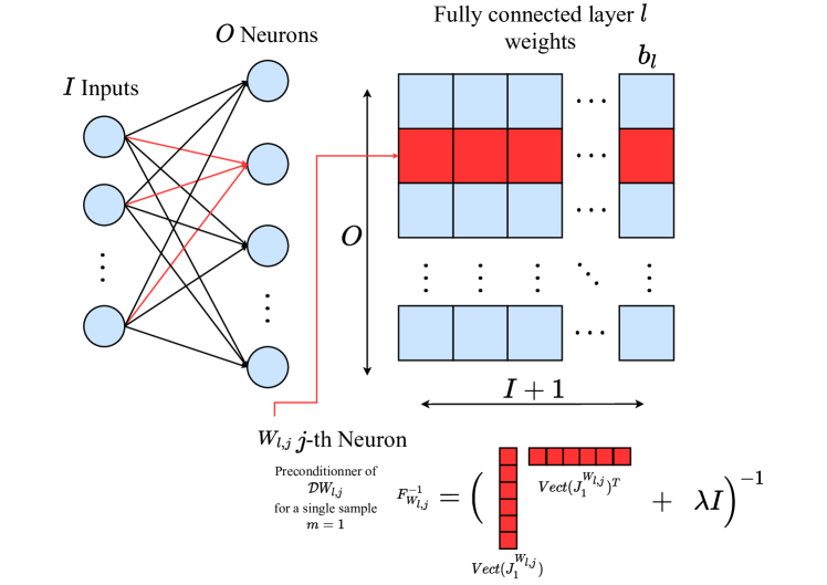
Layer $l$ is feed forward and fully connected (ff-fc): For a ff-fc layer with $I$ inputs and $O$ outputs, we use the following $O\times O$ block-diagonal approximation to the Fisher matrix

$$\bm{F}^{W_{l}}\approx\text{diag}\{\bm{F}^{W_{l,1}},\ldots,\bm{F}^{W_{l,O}}\},$$

whose $j_{th}$ diagonal block $\bm{F}^{W_{l,j}}$ is an $(I+1)\times(I+1)$ symmetric matrix corresponding to the vector $W_{l,j}$ of $I$ weights from all of the input neurons and the bias to the $j_{th}$ output neuron. Therefore, the preconditioning matrix $F^{-1}_{W_{l,j}}$ corresponding to the $j_{th}$ output neuron is given by:

$$F^{-1}_{W_{l,j}}:=\left(\frac{1}{n}(\bm{J}^{W_{l,j}})^{T}\bm{J}^{W_{l,j}}+\lambda I\right)^{-1}$$

Our choice of such a mini-block subdivision was motivated by the findings presented in (Roux et al., 2008), first derived in (Collobert, 2004), where it was shown that the Hessian of a neural network with one hidden layer with cross-entropy loss converges during optimization to a block-diagonal matrix, where the diagonal blocks correspond to the weights linking all the input units to one hidden unit and all of the hidden units to one output unit.

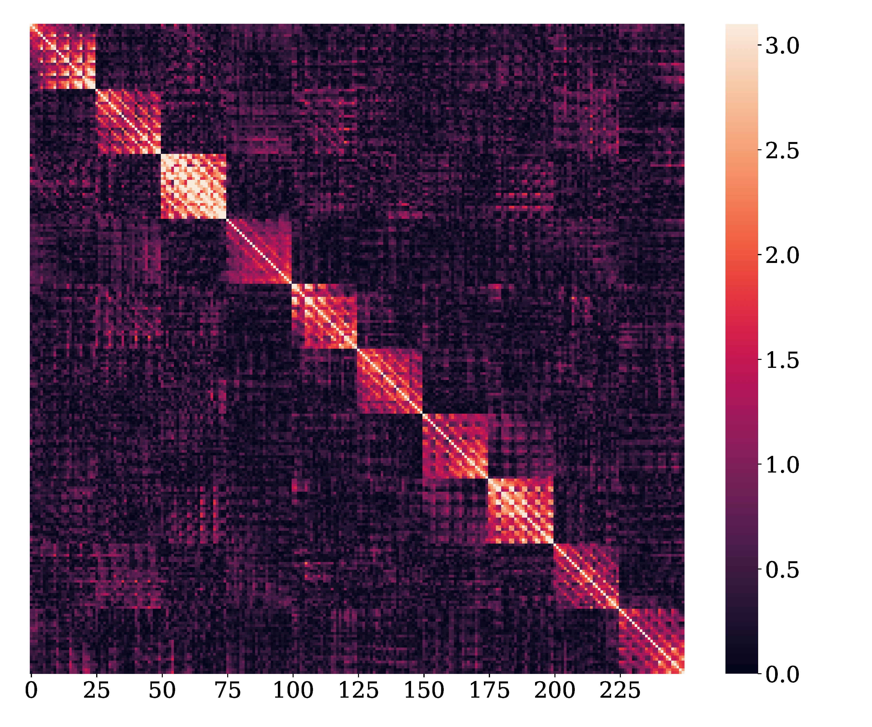
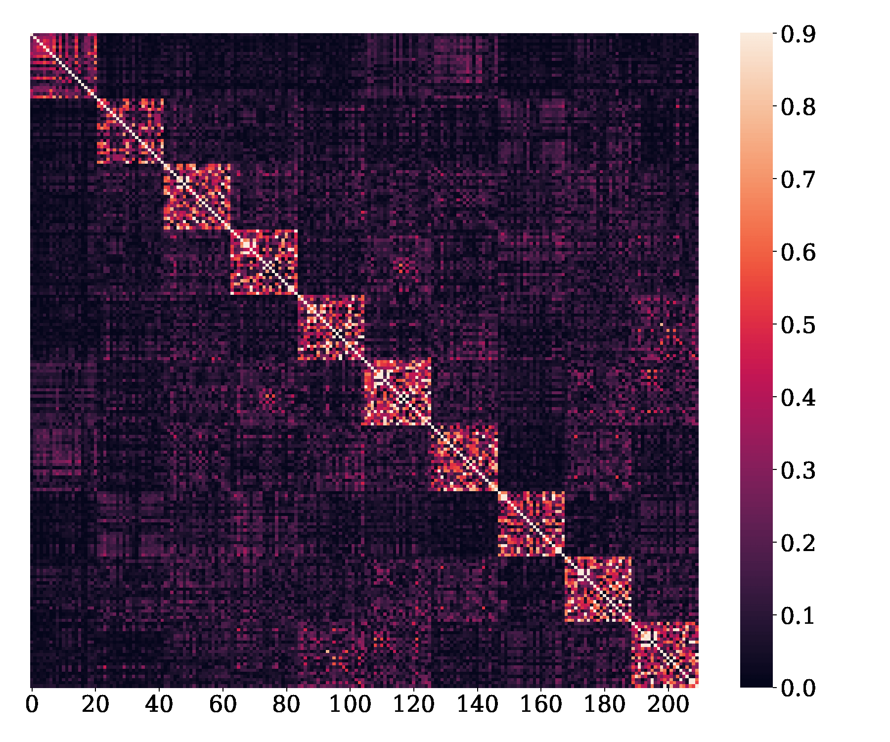
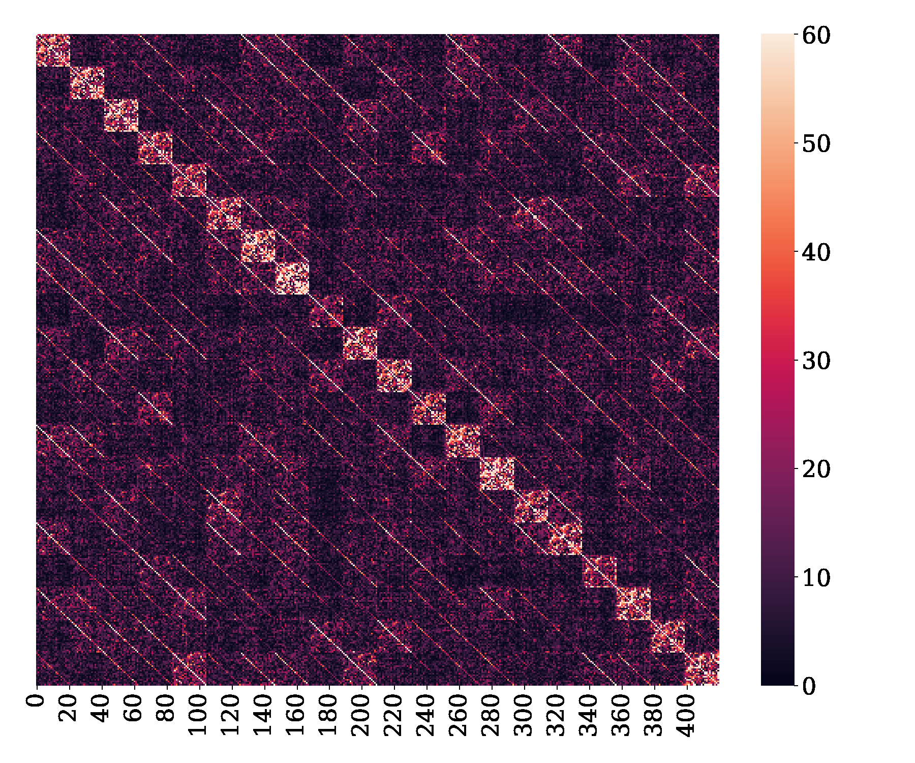
This suggests that a similar block-diagonal structure applies to the Fisher matrix in the limit of a sequence of iterates produced by an optimization algorithm. The latter suggestion was indeed confirmed by findings presented in (ichi Amari et al., 2018), where the authors proved that a "unit-wise" block diagonal approximation to the Fisher information matrix is close to the full matrix modulo off-diagonal blocks of small magnitude, which provides a justification for the quasi-diagonal natural gradient method proposed in (Ollivier, 2015) and our mini-block approximation in the case of fully connected layers. Finally, since the $O$ matrices $\bm{F}^{W_{l,j}}$, for $j=1,\dots,O$, are all of the same size, $(I+1)\times(I+1)$, they can be inverted efficiently by utilizing the parallelism of GPUs. We illustrate MBF’s approximation for a fully connected layer for the case of one data-point in Figure 5 for a $7$-layer (256-20-20-20-20-20-10) feed-forward DNN using $\tanh$ activations, partially trained to classify a $16\times 16$ down-scaled version of MNIST as in (Martens & Grosse, 2015).

Algorithm 1 Generic MBF training algorithm

0:  Given learning rates $\{\alpha_{k}\}$, damping value $\lambda$, batch size $m$

1:  for $k=1,2,...$ do

2:     Sample mini-batch $M$ of size $m$

3:     Perform a forward-backward pass over $M$ to compute stochastic gradient $\mathcal{D}W_{l}$ ($l=1,...,L$)

4:     for $l=1,...,L$ do

5:        for mini-block $b$ in layer $l$, in parallel do

6:           $F^{-1}_{W_{l,b}}:=\left(\frac{1}{m}(\bm{J}^{W_{l,b}})^{T}\bm{J}^{W_{l,b}}+\lambda I\right)^{-1}$

7:           $W_{l,b}=W_{l,b}-\alpha_{k}F^{-1}_{W_{l,b}}\mathcal{D}W_{l,b}$

8:        end for

9:     end for

10:  end for

Algorithm 1 below gives the pseudo-code for a generic version of MBF. Since updating the Fisher mini-blocks is time consuming in practice as it requires storing and computing the individual gradients, we propose in Section 7 below, a practical approach for approximating these matrices. However, we first present empirical results that justify and motivate both the kernel-based and the all-to-one mini-block subdivisions described above for convolutional and ff-fc layers, respectively, followed by a discussion of the linear convergence of an idealized version of the generic MBF algorithm.

After deriving our MBF method, we became aware of the paper (Anil et al., 2021), which proposes using sub-layer block-diagonal preconditioning matrices for Shampoo, a tensor based DNN training method. Specifically, it considers two cases: partitioning (i) very large individual ff-fc matrices (illustrating this for a matrix of size $[2^{9}\times 2^{11}]$ into either a $1\times 2$ or a $2\times 2$ block matrix with blocks all of the same size) and (ii) ResNet-50 layer-wise matrices into sub-layer blocks of size 128. However, (Anil et al., 2021) does not propose a precise method for using mini-blocks as does MBF.

Motivation for MBF:

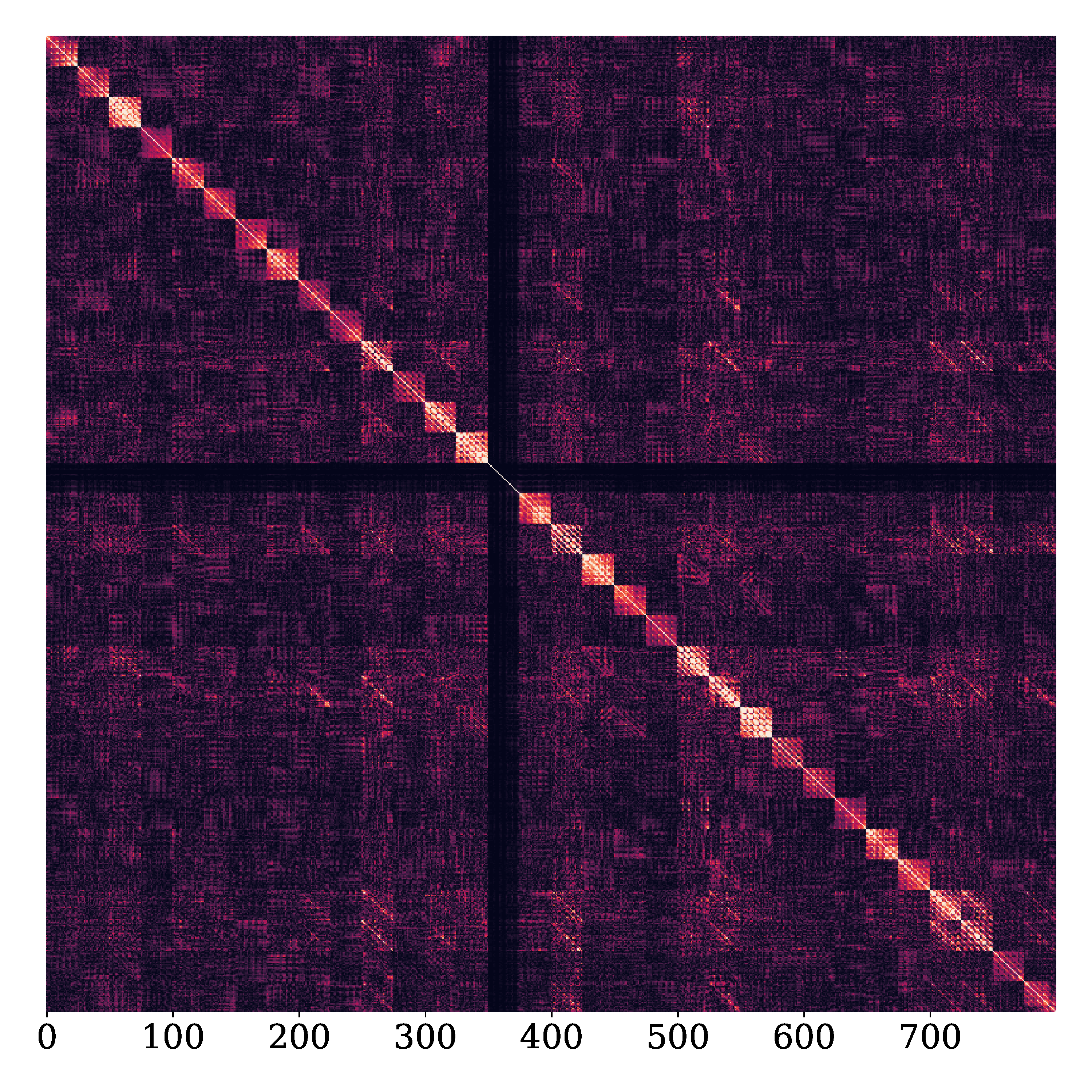
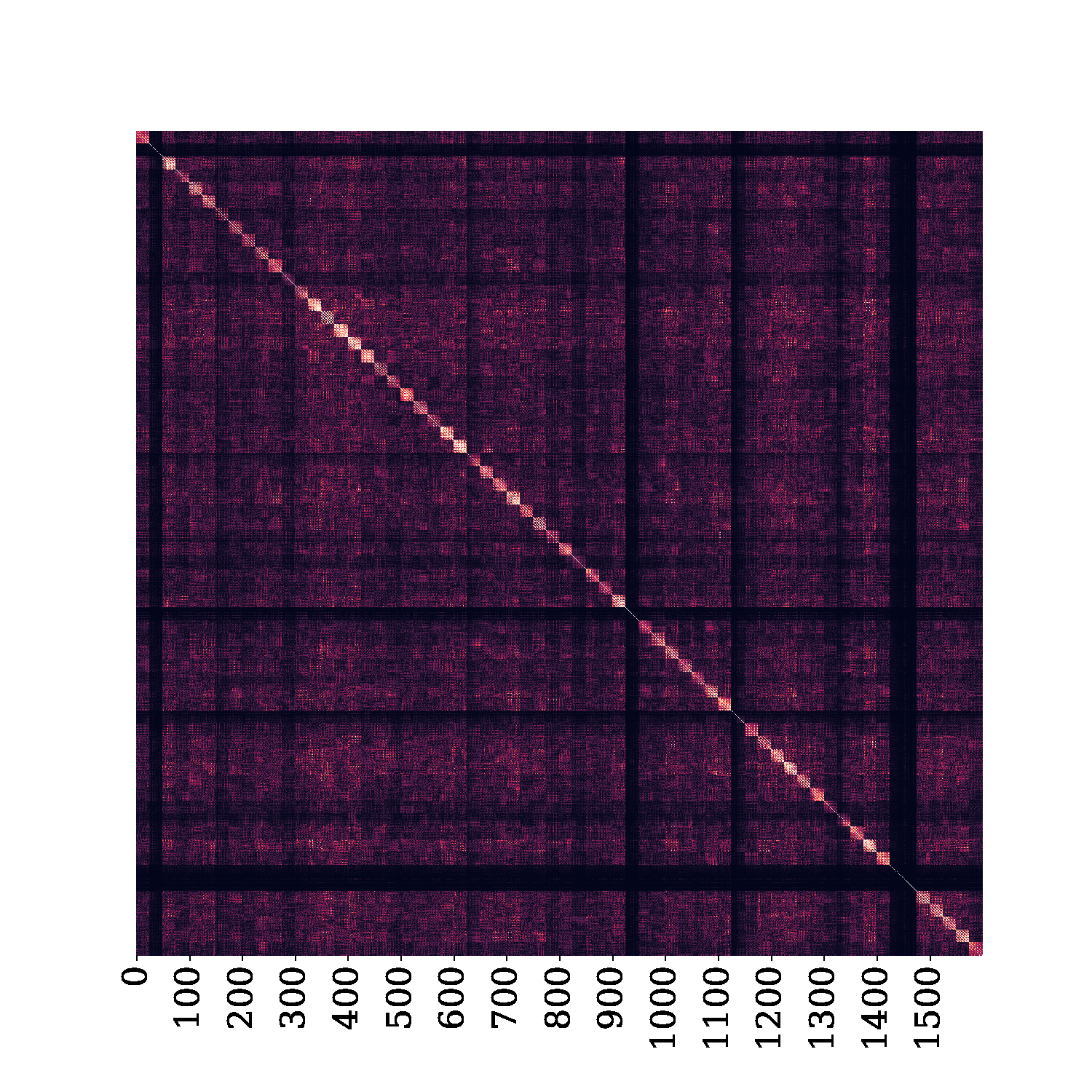
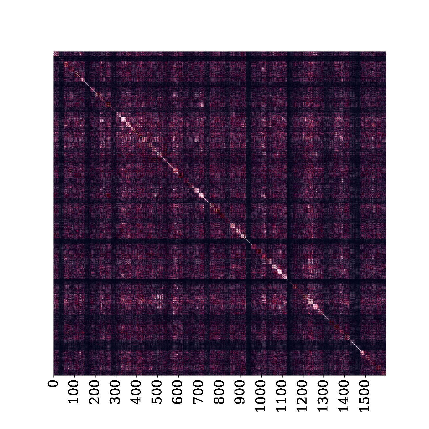
Our choice of mini-blocks for both the convolutional and ff-fc layers was motivated by the observation that most of the weight in the EFM inverse resides in diagonal blocks, and in particular in the mini-blocks described above. More specifically, to illustrate this observation for convolutional layers, we trained a simple convolutional neural network, Simple CNN, (see Appendix 11.4.5 for more details) on Fashion MNIST (Xiao et al., 2017). Figure 5 shows the heatmap of the absolute value of the EFM inverse corresponding to the first convolutional layer, which uses $32$ filters of size $5\times 5$ (thus 32 mini-blocks of size $25\times 25$ ). One can see that the mini-block (by filter) diagonal approximation is reasonable. Figures for the 2nd convolutional layer are included in the Appendix 11.4.5. Since the ff-fc layers in the Simple-CNN model result in an EFM for those layers that is too large to work with, we chose to illustrate the mini-block structure of the EFM on a standard DNN, partially trained to classify a $16\times 16$ down-scaled version of MNIST that was also used in (Martens & Grosse, 2015). Figure 5 shows the heatmap of the absolute value of the EFM inverse for the last and middle fully connected layers (including bias). One can see that the mini-block (by neuron) diagonal approximation is reasonable. A larger figure for the second fully-connected layer is included in Appendix 11.4.5).

(a) First CNN layer

(b) Zoom on first 10 blocks

Figure 4: Absolute EFM inverse after 10 epochs for the first convolutional layer of the Simple CNN network that uses $32$ filters of size $5\times 5$.

(a) Last layer

(b) Middle layer

Figure 5: Absolute EFM inverse after 50 epochs of the last and middle layers (including bias) of a small FCC-NN.

Comparison: directions of MBF and other methods vs. full block-diagonal EFM:

To explore how close is MBF’s direction to the one obtained by a block-diagonal full EFM method (BDF), where each block corresponds to one layer’s full EFM in the model, we computed the cosine similarity between these two directions. We also included SOTA first-order (SGD-m, Adam) and second-order (KFAC, Shampoo) methods for reference. The algorithms were run on a $16\times 16$ down-scaled MNIST (LeCun et al., 2010) dataset and a small feed-forward NN with layer widths 256-20-20-20-20-20-10 described in (Martens & Grosse, 2015). As in (Martens & Grosse, 2015), we only show the middle four layers. For all methods, we followed the trajectory obtained using the BDF method. In our implementation of the BDF method, both the gradient and the block-EMF matrices were estimated with a moving-average scheme, with the decay factors being 0.9. Note that MBF-True refers to the version of MBF in which, similarly to KFAC, the mini-block Fisher is computed by drawing one label from the model distribution for each input image as opposed to MBF, where we use the average over the empirical data. For a more detailed comparison on Autoencoder and CNN problems, see Appendix 11.

As shown in Figure 6, the cosine similarity between the MBF and MBF-True and the BDF direction falls on most iterations between 0.6 to 0.7 for all four layers and not surprisingly, falls midway between the SOTA first-order and block-diagonal second order methods - always better than SGD-m and Adam, but usually lower than that of KFAC and Shampoo. Moreover, the closeness of the plots for MBF and MBF-True shows that using moving average mini-block versions of the EMF rather than the Fisher matrix does not significantly affect the effectiveness of our approach.

We also report a comparison of the performance of MBF-True and MBF on autoencoders and CNN problems in Appendix 11.4.2. Note that, in MBF-True, the only difference between it and MBF is that we are using the mini-batch gradient $\overline{\mathcal{D}_{2}W_{l,b}}$ (denoted by $\mathcal{D}_{2}$) of the model on sampled labels $y_{t}$ from the model’s distribution to update the estimate of mini-block preconditioners, using a moving average (see lines 12, 13 in Algorithm 4 in Appendix 11.4.1), with a rank one outer-product, which is different from computing the true Fisher for that mini-block.

Figure 6: Cosine similarity between the directions produced by the methods shown in the legend and that of a block diagonal Fisher method (BDF).

4 Linear Convergence

We follow the framework established in (Zhang, Martens & Grosse, 2019) to provide convergence guarantees for the idealized MBF with exact gradients (i.e. full batch case with $m=n$) and the min-block version of the true Fisher matrix, rather than the EFM, as the underlying preconditioning matrix. We focus on the single-output case with squared error loss, but analysis of the multiple-output case is similar.

We denote by $\textbf{ {u}}(\bm{W})=[f(\bm{W},x_{1}),...,f(\bm{W},x_{n})]^{\top}$ the output vector and $y=[{y}_{1},...,{y}_{n}]^{\top}$ the true labels. We consider the squared error loss $\mathcal{L}$ on a given data-set $\{x_{i},y_{i}\}_{i=1}^{n}$ with $x_{i}\in\mathbb{R}^{d}$ and $y_{i}\in\mathbb{R}$, i.e. the objective is to minimize

$$\min_{\bm{W}\in\mathbb{R}^{p}}\mathcal{L}(\bm{W})=\frac{1}{2}\|\textbf{ {u}}(\bm{W})-y\|^{2}.$$

The update rule of MBF with exact gradient becomes

where $\bm{F}_{MB}(\bm{W}(k)):=\frac{1}{n}\bm{J}_{MB}(\bm{W}(k))^{\top}\bm{J}_{MB}(\bm{W}(k))$ is the mini-block-Fisher matrix and the mini-block Jacobian is defined as $\bm{J}_{MB}(k)=\text{Diag}_{l\in[L]}\text{Diag}_{b}\left(J^{\bm{W}_{l,b}}(k)\right)$ and

$$J^{\bm{W}_{l,b}}(k):=[\frac{\partial f(\bm{W}(k),\textbf{x}_{1})}{\partial\bm{W}_{l,b}},...,\frac{\partial f(\bm{W}(k),\textbf{x}_{n})}{\partial\bm{W}_{l,b}}]^{\top}$$

We use similar assumptions to those used in (Zhang, Martens & Grosse, 2019), where the first assumption, ensures that at initialization, the mini-block Gram matrices are all positive-definite, (i.e., the rows of their respective Jacobians are linearly independent), and the second assumption ensures the stability of the Jacobians by requiring that the network is close to a linearized network at initialization and therefore MBF’s update is close to the gradient descent direction in the output space. These assumptions allow us to control the convergence rate.

Assumption 4.1.

The mini-block Gram matrices $J^{\bm{W}_{l,b}}(0)J^{\bm{W}_{l,b}}(0)^{T}$ at initialization are positive definite, i.e. $\min_{l\in[L]}\min_{b}\lambda_{min}(J^{\bm{W}_{l,b}}(0)^{T}J^{\bm{W}_{l,b}}(0))=\lambda_{0}>0$.

Assumption 4.2.

There exists $0<C\leq\frac{1}{2}$ that satisfies $\|{\bm{J}(\bm{W}(k))}-\bm{J}(\bm{W}(0))\|_{2}\leq\frac{C}{3}\sqrt{\lambda_{0}}$ if $\|\bm{W}(k)-\bm{W}(0)\|_{2}\leq\frac{3}{\sqrt{\lambda_{0}}}\|\bm{y}-\bm{u}(0)\|_{2}$.

Theorem 1.

Suppose Assumptions 4.1, 4.2 hold. Consider the Generic BMF Algorithm 1, using exact gradients and the mini-block version of the true Fisher as the underlying preconditioning matrix for a network with $L$ layers. Then there exists an interval of suitable damping values $\lambda$ in $[\underline{\lambda},\overline{\lambda}]$ and corresponding small enough learning rates $\eta_{\lambda}$, such that for any learning rate $0\leq\eta\leq\eta_{\lambda}$ we have ${\|\textbf{ {u}}(\bm{W}(k))-\textbf{ {y}}\|_{2}^{2}\leq(1-\eta)^{k}\|\textbf{ {u}}(\bm{W}(0))-\textbf{ {y}}\|_{2}^{2}.}$

Theorem 1 states that an idealized verion of MBF converges to the global optimum with a linear rate under Assumptions 4.1 and 4.2. Our analysis is an adaptation of the proof in (Zhang, Martens & Grosse, 2019), where we first exploit Assumptions 4.1 and 4.2 to obtain a positive lower bound on the eigenvalues of mini-block version of the true Fisher matrix $\bm{F}_{MB}(\bm{W}(k))$, which then allows us to characterize the rate of convergence of the method. The proof can be found in the Appendix 9.

5 Implementation Details of MBF and Comparison on Complexity

Mini-batch averages, Exponentially decaying averages and Momentum: Because the size of training data sets is usually large, we use mini-batches to estimate the quantities needed for MBF. We use $\overline{X}$ to denote the average value of $X$ over a mini-batch for any quantity $X$. Moreover, for the EFM mini-blocks, we use moving averages to both reduce the stochasticity and incorporate more information from the past, more specifically, we use a moving average scheme to get a better estimate of the EFM mini-blocks, i.e.$\widehat{G_{W_{l,b}}}=\beta\widehat{G_{W_{l,b}}}+(1-\beta)\overline{G_{W_{l,b}}},$ where $\overline{G_{W_{l,b}}}$ is the current approximation to the mini-block EFM defined below. In order to bring MBF closer to a drop-in replacement for adaptive gradient methods such as Adam, we add momentum to the mini-batch gradient, let: $\widehat{\mathcal{D}W_{l}}=\mu\widehat{\mathcal{D}W_{l}}+\overline{\mathcal{D}W_{l}}$ and then apply the preconditioner to $\widehat{\mathcal{D}W_{l}}$ to compute the step.

Approximating the mini-block Fisher matrices: As mentioned previously, computing the matrices $\overline{G_{W_{l,b}}}:=\frac{1}{m}(\bm{J}^{W_{l,b}})^{T}\bm{J}^{W_{l,b}}$ to update the EFM mini-blocks is inefficient in practice as this requires storing and computing the individual gradients. Hence, we approximate these mini-block matrices by the outer product of the part of the mini-batch gradient corresponding to the subset of weights $W_{l,b}$, i.e., $\overline{G_{W_{l,b}}}\approx(\overline{\mathcal{D}W_{l,b}})(\overline{\mathcal{D}W_{l,b}})^{\top}$.

Spacial average for large fully-connected layers: In some CNN and autoencoder models, using the EFM mini-blocks can still be computationally prohibitive for fc layers, where both the input and output dimensions are large. Therefore, for such layers we used a Spatial Averaging technique, similar to one used in (Yao et al., 2021), where we maintained a single preconditioning matrix for all the mini-blocks by averaging the approximate mini-block EFM matrices whenever we updated the preconditioning matrix. This technique also leads to more stable curvature updates as a side benefit, as observed for the method proposed in (Yao et al., 2021), where the Hessian diagonal was "smoothed" across each layer. We also explored using spacial averaging for convolutional layers. However since the kernel-wise mini-blocks are small in size, spacial averaging doesn’t compare favorably to the full MBF method (see Appendix 11.4.3).

Amortized updates of the preconditioning matrices: The extra work for the above computations, as well as for updating the inverses $F^{-1}_{W_{l,j}}$ compared with first-order methods is amortized by only performing the Fisher matrix updates every $T_{1}$ iterations and computing their inverses every $T_{2}$ iterations. This approach which is also used in KFAC and Shampoo, does not seem to degrade MBF’s overall performance, in terms of computational speed.

Comparison of Memory and Per-iteration Time Complexity. In Table 1, we compare the space and computational requirements of the proposed MBF method with KFAC (see Appendix 11.1) and Adam, which are among the predominant 2nd and 1st-order methods, respectively, used to train DNNs. We focus on one convolutional layer, with $J$ input channels, $I$ output channels, kernel size $|\Delta|=(2R+1)^{2}$, and $|\mathcal{T}|$ spacial locations. Let $m$ denote the size of the minibatches, and $T_{1}$ and $T_{2}$ denote, respectively, the frequency for updating the preconditioners and inverting them for both KFAC and MBF. As indicated in Table 1, the amount of memory required by MBF is the same order of magnitude as that required by Adam, (specifically, more by a factor of $|\Delta|$, which is usually small in most CNN architectures; e.g, in VGG16 (Simonyan & Zisserman, 2014) $|\Delta|=9$) and less than KFAC, Shampoo and other SOTA Kronecker-factored preconditioners, (specifically, e.g., by a factor of $O\left(J+\frac{I}{|\Delta|}\right)$ for KFAC.

We can also see that MBF requires only a small amount more per-iteration time than Adam (i.e., by a factor of $\left(\frac{|\Delta|}{T_{1}}+\frac{|\Delta|^{2}}{T_{2}}+|\Delta|\right)$). Note that in our experiments, $T_{1}\approx|\Delta|$ and $T_{2}\approx|\Delta|^{2}$. The computationnal and storage requirements for fully connected layers are discussed in Appendix 11.1.5. Our MBF algorithm is described fully as Algorithm 2 in the Appendix 8.

Table 1: Computation and Storage Requirements per iteration for convolutional layer.

Algorithm	Additional pass	Curvature	Step $\Delta W_{l}$	Storage $P_{l}$
MBF	—	$O(\frac{IJ|\Delta|^{2}}{T_{1}}+\frac{IJ|\Delta|^{3}}{T_{2}})$	$O(IJ|\Delta|^{2})$	$O(IJ|\Delta|^{2})$
Shampoo	—	$O(\frac{(J^{2}+|\Delta|^{2}+I^{2})}{T_{1}}+\frac{J^{3}+I^{3}+|\Delta|^{3}}{T_{2}})$	$O((I+J+|\Delta|)IJ|\Delta|)$	$O(I^{2}+J^{2}+|\Delta|^{2})$
KFAC	$O(\frac{mIJ|\Delta||\mathcal{T}|}{T_{1}})$	$O(\frac{m(J^{2}|\Delta|^{2}+I^{2})|\mathcal{T}|}{T_{1}}+\frac{J^{3}|\Delta|^{3}+I^{3}}{T_{2}})$	$O(IJ^{2}|\Delta|^{2}+I^{2}J|\Delta|)$	$O(J^{2}|\Delta|^{2}+I^{2})$
Adam	—	$O(IJ|\Delta|)$	$O(IJ|\Delta|)$	$O(IJ|\Delta|)$

6 Experiments

In this section, we compare MBF with some SOTA first-order (SGD-m, Adam) and second-order (KFAC, Shampoo) methods. (See Appendix 11.1 on how these methods were implemented.) Since MBF uses information about the second-moment of the gradient to construct a preconditioning matrix, Adam, KFAC and Shampoo were obvious choices for comparison with MBF.

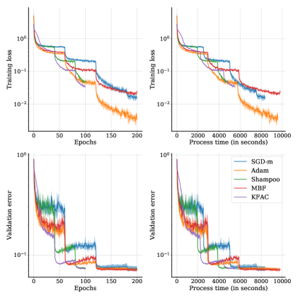
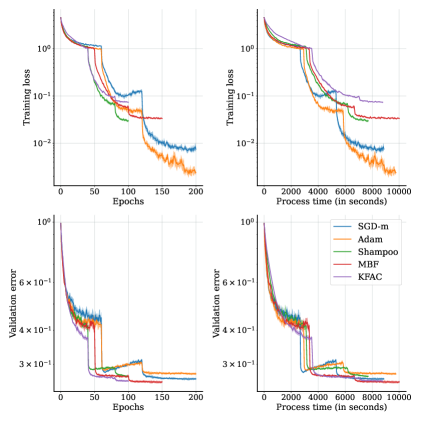
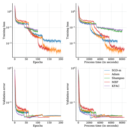
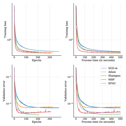
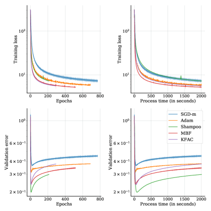
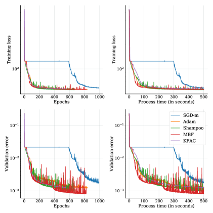
Our experiments were run on a machine with one V100 GPU and eight Xeon Gold 6248 CPUs using PyTorch Paszke et al. (2019). Each algorithm was run using the best hyper-parameters, determined by a grid search (specified in Appendices 11.3 and 11.2), and 5 different random seeds. The performance of MBF and the comparison algorithms is plotted in Figures 7 and 8: the solid curves depict the results averaged over the 5 different runs, and the shaded areas depict the $\pm$standard deviation range for these runs.

Generalization performance, CNN problems:

We first compared the generalization performance of MBF to SGD-m, Adam, KFAC and Shampoo on three CNN models, namely, ResNet32 He et al. (2016), VGG16 Simonyan & Zisserman (2014) and VGG11 Simonyan & Zisserman (2014), respectively, on the datasets CIFAR-10, CIFAR-100 and SVHN Krizhevsky et al. (2009). The first two have 50,000 training data and 10,000 testing data (used as the validation set in our experiments), while SVHN has 73,257 training data and 26,032 testing data. For all algorithms, we used a batch size of 128. In training, we applied data augmentation as described in Krizhevsky et al. (2012), including random horizontal flip and random crop, since these setting choices have been used and endorsed in many previous research papers, e.g. Zhang, Wang, Xu & Grosse (2019); Choi et al. (2019); Ren & Goldfarb (2021b). (see Appendix 11 for more details about the experimental set-up)

On all three model/dataset problems, the first-order methods were run for 200 epochs, and KFAC and Shampoo for 100 epochs, while MBF was run for 150 epochs on VGG16/CIFAR-100 and VGG11/SVHN, and 200 epochs on ResNet32/CIFAR-10. The reason that we ran MBF for 200 epochs (i.e., the same number as run for Adam) on ResNet32 was because all of ResNet32’s convolutional layers use small ($3\times 3$) kernels, and it contains just one fully connected layer of modest size $(I,O)=(64,10)$. Hence as we expected, MBF and Adam took almost the same time to complete 200 epochs. As can be seen in Figure 7, MBF could have been terminated after 150 epochs, without a significant change in validation error. On the other hand, since VGG16 and VGG11 have two large fully connected-layers (e.g [4096, 4096, 10/100]), MBF’s per-iteration computational cost is substantially larger than Adam’s due to these layers. Consequently, for both methods to finish roughly in the same amount of time, we ran MBF for only 150 epochs.

All methods employed a learning rate (LR) schedule that decayed LR by a factor of 0.1 every K epochs, where K was set to 40, 50 and 60, for the first-order methods, MBF, and KFAC/Shampoo, respectively, on the VGG16 and VGG11 problems, and set to 40, 60, and 80, respectively, on the ResNet32 problem

Moreover, weight decay, which has been shown to improve generalization across different optimizers Loshchilov & Hutter (2019); Zhang, Wang, Xu & Grosse (2019), was employed by all of the algorithms, and a grid search on the weight decay factor and the initial learning rate based on the criteria of maximal validation classification accuracy, was performed. Finally, the damping parameter was set to 1e-8 for Adam (following common practice), and 0.03 for KFAC (https://github.com/alecwangcq/KFAC-Pytorch). For Shampoo, we set $\epsilon=0.01$. For MBF, we set $\lambda=0.003$. We set $T_{1}=10$ and $T_{2}=100$ for KFAC, Shampoo and MBF.

From Figure 7, we see that MBF has a similar (and sometimes better) generalization performance than the other methods. Moreover, in terms of process time, MBF is roughly as fast as SGD-m and Adam on ResNet32/CIFAR-10 in Figure 7, and is competitive with all of the SOTA first and second-order methods in our experiments.

(a) CIFAR-10, ResNet-32

(b) CIFAR-100, VGG16

(c) SVHN, VGG11

Figure 7: Generalization ability of MBF, KFAC, Shampoo, Adam, and SGD-m on three CNN problems.

Optimization performance, Autoencoder Problems:

We also compared the optimization performance of the algorithms on three autoencoder problems Hinton & Salakhutdinov (2006) with datasets MNIST LeCun et al. (2010), FACES, and CURVES, which were also used for benchmarking algorithms in Martens (2010); Martens & Grosse (2015); Botev et al. (2017); Goldfarb et al. (2020). The details of the layer shapes of the autoencoders are specified in Appendix 11.2. For all algorithms, we used a batch size of 1,000, and settings that largely mimic the settings in the latter papers. Each algorithm was run for 500 seconds for MNIST and CURVES, and 2000 seconds for FACES.

For each algorithm, we conducted a grid search on the LR and damping value based on minimizing the training loss. We set the Fisher matrix update frequency $T_{1}=1$ and inverse update frequency $T_{2}=20$ for second-order methods, as in Ren & Goldfarb (2021b). From Figure 8, it is clear that MBF outperformed SGD-m and Adam, both in terms of per-epoch progress and process time. Moreover, MBF performed (at least) as well as KFAC and Shampoo. We postulate that the performance of MBF is due to its ability to capture important curvature information from the mini-block Fisher matrix, while keeping the computational cost per iteration low and close to that of Adam.

(a) MNIST autoencoder

(b) FACES autoencoder

(c) CURVES autoencoder

Figure 8: Optimization performance of MBF, KFAC, Shampoo, Adam, and SGD-m on three autoencoder problems.

7 Conclusion and Future Research

We proposed a new EMF-based method, MBF, for training DNNs, by approximating the EMF by a mini-block diagonal matrix that arises naturally from the structure of convolutional and ff-fc layers. MBF requires very mild memory and computational overheads, compared with first-order methods, and is easy to implement. Our experiments on various DNNs and datasets, demonstrate conclusively that MBF provides comparable and sometimes better results than SOTA methods, both from an optimization and generalization perspective. Future research will investigate extending MBF to other deep learning architectures such as Recurrent neural networks.

 

Supplementary Materials for "A Mini-Block Fisher Method for Deep Neural Networks"

 

8 MBF Full implementation

We present below pseudo-code for the full detailed implementation of our MBF algorithm thatwe us ed in producing the results in the main text.

Algorithm 2 Mini-Block Fisher method (MBF)

0:  Given batch size $m$, learning rate $\{\eta_{k}\}_{k\geq 1}$, weight decay factor $\gamma$, damping value $\lambda$, statistics update frequency $T_{1}$, inverse update frequency $T_{2}$

1:  $\mu=0.9$, $\beta=0.9$

2:  Initialize $\widehat{G_{l,b}}=\mathbb{E}[G_{l,b}]$ ($l=1,..,k$, mini-blocks $b$) by iterating through the whole dataset, $\widehat{\mathcal{D}W_{l,b}}=0$ ($l=1,..,k$, mini-blocks $b$)

3:  for $k=1,2,\ldots$ do

4:     Sample mini-batch $M_{t}$ of size $m$

5:     Perform a forward-backward pass over $M_{t}$ to compute the mini-batch gradient $\overline{\mathcal{D}W_{l,b}}$

6:     for $l=1,...L$ do

7:        for mini-block $b$ in layer $l$, in parallel do

8:           $\widehat{\mathcal{D}W_{l,b}}=\mu\widehat{\mathcal{D}W_{l,b}}+\overline{\mathcal{D}W_{l,b}}$

9:           if $k\equiv 0\pmod{T_{1}}$ then

10:              If Layer $l$ is convolutional: $\widehat{G_{l,j,i}}=\beta\widehat{G_{l,j,i}}+(1-\beta)\overline{\mathcal{D}W_{l,j,i}}\left(\overline{\mathcal{D}W_{l,j,i}}\right)^{\top}$

11:              If Layer $l$ is fully-connected: $\widehat{G_{l}}=\beta\widehat{G_{l}}+\frac{1-\beta}{O}\sum_{j=1}^{O}\overline{\mathcal{D}W_{l,j}}\left(\overline{\mathcal{D}W_{l,j}}\right)^{\top}$

12:           end if

13:           if $k\equiv 0\pmod{T_{2}}$ then

14:              Recompute and store $(\widehat{G_{l,b}}+\lambda I)^{-1}$

15:           end if

16:           $p_{l,b}=(\widehat{G_{l,b}}+\lambda I)^{-1}\widehat{\mathcal{D}W_{l,b}}+\gamma W_{l,b}$

17:           $W_{l,b}=W_{l,b}-\eta_{k}p_{l,b}$

18:        end for

19:     end for

20:  end for

9 Proof of Convergence of Algorithm MBF and Associated Lemmas

We follow the framework used in Zhang, Martens & Grosse (2019) to prove linear convergence of NG descent, to provide similar convergence guarantees for our idealized MBF Algorithm, that uses exact gradients (i.e. full batch case with $m=n$) and the mini-block version of the true Fisher as the underlying preconditioning matrix.

Proof of Theorem 1. If Assumption 6.2 holds, then one can obtain a lower bound on the minimum eigenvalue of the mini-block Fisher matrix $\bm{F}_{MB}(\bm{W}(k))=\frac{1}{n}\bm{J}_{MB}(k)^{\top}\bm{J}_{MB}(k)$ at each iteration.

In fact, if $\|\bm{W}(k)-\bm{W}(0)\|_{2}\leq\frac{3}{\sqrt{\lambda_{0}}}\|\bm{y}-\bm{u}(0)\|_{2}$, then, by Assumption 6.2, there exists $0<C\leq\frac{1}{2}$ that satisfies $\|{\bm{J}(\bm{W}(k))}-\bm{J}(\bm{W}(0))\|_{2}\leq\frac{C}{3}\sqrt{\lambda_{0}}$, and therefore, we have that

$$\|\bm{J}_{MB}(k)-\bm{J}_{MB}(0)\|_{2}\leq\frac{C\sqrt{\lambda_{0}}}{3}\leq\frac{\sqrt{\lambda_{0}}}{3}.$$

On the other hand, based on the inequality $\sigma_{\min}(\mathbf{A}+\mathbf{B})\geq\sigma_{\min}(\mathbf{A})-\sigma_{\max}(\mathbf{B})$, where $\sigma$ denotes singular value, we have

$$\sigma_{\min}(\bm{J}_{MB}(k)) \geq\sigma_{\min}(\bm{J}_{MB}(0))-\sigma_{\min}(\bm{J}_{MB}(k)-(\bm{J}_{MB}(k)))$$

$$\geq\sigma_{\min}(\bm{J}_{MB}(0))-\|\bm{J}_{MB}(k)-\bm{J}_{MB}(0)\|_{2}\geq\sqrt{\lambda_{0}}-\frac{\sqrt{\lambda_{0}}}{3}=\frac{2\sqrt{\lambda_{0}}}{3}.$$

Therefore

$$\lambda_{min}(\bm{G}_{MB}(\bm{W}(k)))\geq\frac{4\sqrt{\lambda_{0}}}{9}.$$

where $\bm{G}_{MB}(\bm{W}(k)):=\bm{J}_{MB}(\bm{W}(k))\bm{J}_{MB}(\bm{W}(k))^{\top}$ is the mini-block Gram matrix. We prove Theorem 1 by induction. Assume $||\textbf{ {u}}(\bm{W}(k))-\bm{y}||_{2}^{2}\leq(1-\eta)^{k}||\textbf{ {u}}(\bm{W}(0))-\textbf{ {y}}||_{2}^{2}$. One can see that the relationship between the Jacobian $\bm{J}(\bm{W}(k))$ and the mini-Block Jacobian $\bm{J}_{MB}(\bm{W}(k))$ is:

$$\bm{J}^{\top}(\bm{W}(k))=\bm{J}_{MB}(\bm{W}(k))^{\top}\bm{K},$$

where the matrix $\bm{K}=\underbrace{[I_{n},\dots,I_{n}]^{\top}}_{K}\in\mathbb{R}^{Kn\times n}$, $I_{n}$ is the identity matrix of dimension $n$, the number of samples, and $K$ is the total number of mini-blocks. We define

$$\bm{W}_{k}(s) =s\bm{W}(k+1)+(1-s)\bm{W}(k)$$

$$=\bm{W}(k)-s\frac{\eta}{n}\left(\bm{F}_{MB}(\bm{W}(k))+\lambda I\right)^{-1}\bm{J}(\bm{W}(k))^{\top}(\textbf{ {u}}(\bm{W}(k))-\bm{y}))-\textbf{ {u}}(\bm{W}(k)),$$

we have:

$$\textbf{ {u}}(\bm{W}(k+1))-\textbf{ {u}}(\bm{W}(k))$$

$$=\bm{u}(\bm{W}(k)-\frac{\eta}{n}\left(\bm{F}_{MB}(\bm{W}(k))+\lambda I\right)^{-1}\bm{J}(\bm{W}(k))^{\top}(\textbf{ {u}}(\bm{W}(k))-\bm{y}))-\textbf{ {u}}(\bm{W}(k))$$

$$=-\int_{s=0}^{1}\Big{\langle}\frac{\partial\bm{u}(\bm{W}_{k}(s))}{\partial\bm{W}^{\top}},\frac{\eta}{n}\left(\bm{F}_{MB}(\bm{W}(k))+\lambda I\right)^{-1}\bm{J}(\bm{W}(k))^{\top}(\bm{u}(\bm{W}(k))-\bm{y}))\Big{\rangle}ds$$

$$=-\underbrace{\int_{s=0}^{1}\Big{\langle}\frac{\partial\bm{u}(\bm{W}(k))}{\partial\bm{W}^{\top}},\frac{\eta}{n}\left(\bm{F}_{MB}(\bm{W}(k))+\lambda I\right)^{-1}\bm{J}(\bm{W}(k))^{\top}(\bm{u}(\bm{W}(k))-\bm{y}))\Big{\rangle}ds}_{\leavevmode\hbox to13.13pt{\vbox to13.13pt{\pgfpicture\makeatletter\hbox{\hskip 6.56548pt\lower-6.56548pt\hbox to0.0pt{\pgfsys@beginscope\pgfsys@invoke{ }\definecolor{pgfstrokecolor}{rgb}{0,0,0}\pgfsys@color@rgb@stroke{0}{0}{0}\pgfsys@invoke{ }\pgfsys@color@rgb@fill{0}{0}{0}\pgfsys@invoke{ }\pgfsys@setlinewidth{0.4pt}\pgfsys@invoke{ }\nullfont\hbox to0.0pt{\pgfsys@beginscope\pgfsys@invoke{ }{{{}}\hbox{\hbox{{\pgfsys@beginscope\pgfsys@invoke{ }{{}{{{}}}{{}}{}{}{}{}{}{}{}{}{}{{}\pgfsys@moveto{6.36548pt}{0.0pt}\pgfsys@curveto{6.36548pt}{3.5156pt}{3.5156pt}{6.36548pt}{0.0pt}{6.36548pt}\pgfsys@curveto{-3.5156pt}{6.36548pt}{-6.36548pt}{3.5156pt}{-6.36548pt}{0.0pt}\pgfsys@curveto{-6.36548pt}{-3.5156pt}{-3.5156pt}{-6.36548pt}{0.0pt}{-6.36548pt}\pgfsys@curveto{3.5156pt}{-6.36548pt}{6.36548pt}{-3.5156pt}{6.36548pt}{0.0pt}\pgfsys@closepath\pgfsys@moveto{0.0pt}{0.0pt}\pgfsys@stroke\pgfsys@invoke{ } }{{{{}}\pgfsys@beginscope\pgfsys@invoke{ }\pgfsys@transformcm{1.0}{0.0}{0.0}{1.0}{-2.625pt}{-2.39166pt}\pgfsys@invoke{ }\hbox{{\definecolor{pgfstrokecolor}{rgb}{0,0,0}\pgfsys@color@rgb@stroke{0}{0}{0}\pgfsys@invoke{ }\pgfsys@color@rgb@fill{0}{0}{0}\pgfsys@invoke{ }\hbox{{A}} }}\pgfsys@invoke{\lxSVG@closescope }\pgfsys@endscope}}} \pgfsys@invoke{\lxSVG@closescope }\pgfsys@endscope}}} } \pgfsys@invoke{\lxSVG@closescope }\pgfsys@endscope{{{}}}{}{}\hss}\pgfsys@discardpath\pgfsys@invoke{\lxSVG@closescope }\pgfsys@endscope\hss}}\lxSVG@closescope\endpgfpicture}}}$$

$$+\underbrace{\int_{s=0}^{1}\Big{\langle}\frac{\partial\bm{u}(\bm{W}(k))}{\partial\bm{W}^{\top}}-\frac{\partial\bm{u}(\bm{W}_{k}(s))}{\partial\bm{W}^{\top}},\frac{\eta}{n}\left(\bm{F}_{MB}(\bm{W}(k))+\lambda I\right)^{-1}\bm{J}(\bm{W}(k))^{\top}(\bm{u}(\bm{W}(k))-\bm{y}))\Big{\rangle}ds}_{\leavevmode\hbox to12.93pt{\vbox to12.93pt{\pgfpicture\makeatletter\hbox{\hskip 6.46587pt\lower-6.46587pt\hbox to0.0pt{\pgfsys@beginscope\pgfsys@invoke{ }\definecolor{pgfstrokecolor}{rgb}{0,0,0}\pgfsys@color@rgb@stroke{0}{0}{0}\pgfsys@invoke{ }\pgfsys@color@rgb@fill{0}{0}{0}\pgfsys@invoke{ }\pgfsys@setlinewidth{0.4pt}\pgfsys@invoke{ }\nullfont\hbox to0.0pt{\pgfsys@beginscope\pgfsys@invoke{ }{{{}}\hbox{\hbox{{\pgfsys@beginscope\pgfsys@invoke{ }{{}{{{}}}{{}}{}{}{}{}{}{}{}{}{}{{}\pgfsys@moveto{6.26587pt}{0.0pt}\pgfsys@curveto{6.26587pt}{3.46059pt}{3.46059pt}{6.26587pt}{0.0pt}{6.26587pt}\pgfsys@curveto{-3.46059pt}{6.26587pt}{-6.26587pt}{3.46059pt}{-6.26587pt}{0.0pt}\pgfsys@curveto{-6.26587pt}{-3.46059pt}{-3.46059pt}{-6.26587pt}{0.0pt}{-6.26587pt}\pgfsys@curveto{3.46059pt}{-6.26587pt}{6.26587pt}{-3.46059pt}{6.26587pt}{0.0pt}\pgfsys@closepath\pgfsys@moveto{0.0pt}{0.0pt}\pgfsys@stroke\pgfsys@invoke{ } }{{{{}}\pgfsys@beginscope\pgfsys@invoke{ }\pgfsys@transformcm{1.0}{0.0}{0.0}{1.0}{-2.47917pt}{-2.39166pt}\pgfsys@invoke{ }\hbox{{\definecolor{pgfstrokecolor}{rgb}{0,0,0}\pgfsys@color@rgb@stroke{0}{0}{0}\pgfsys@invoke{ }\pgfsys@color@rgb@fill{0}{0}{0}\pgfsys@invoke{ }\hbox{{B}} }}\pgfsys@invoke{\lxSVG@closescope }\pgfsys@endscope}}} \pgfsys@invoke{\lxSVG@closescope }\pgfsys@endscope}}} } \pgfsys@invoke{\lxSVG@closescope }\pgfsys@endscope{{{}}}{}{}\hss}\pgfsys@discardpath\pgfsys@invoke{\lxSVG@closescope }\pgfsys@endscope\hss}}\lxSVG@closescope\endpgfpicture}}}$$

In what follows, to simplify the notation, we drop $\bm{W}(k)$ whenever the context is clear. Thus, we have

$$=\frac{\eta}{n}\bm{J}\left(\bm{F}_{MB}+\lambda I\right)^{-1}\bm{J}^{\top}(\bm{y}-\bm{u}(k)).$$ (3)

Now, we bound the norm of :

$$||\leavevmode\hbox to15.9pt{\vbox to15.9pt{\pgfpicture\makeatletter\hbox{\hskip 7.9522pt\lower-7.9522pt\hbox to0.0pt{\pgfsys@beginscope\pgfsys@invoke{ }\definecolor{pgfstrokecolor}{rgb}{0,0,0}\pgfsys@color@rgb@stroke{0}{0}{0}\pgfsys@invoke{ }\pgfsys@color@rgb@fill{0}{0}{0}\pgfsys@invoke{ }\pgfsys@setlinewidth{0.4pt}\pgfsys@invoke{ }\nullfont\hbox to0.0pt{\pgfsys@beginscope\pgfsys@invoke{ }{{{}}\hbox{\hbox{{\pgfsys@beginscope\pgfsys@invoke{ }{{}{{{}}}{{}}{}{}{}{}{}{}{}{}{}{{}\pgfsys@moveto{7.7522pt}{0.0pt}\pgfsys@curveto{7.7522pt}{4.28146pt}{4.28146pt}{7.7522pt}{0.0pt}{7.7522pt}\pgfsys@curveto{-4.28146pt}{7.7522pt}{-7.7522pt}{4.28146pt}{-7.7522pt}{0.0pt}\pgfsys@curveto{-7.7522pt}{-4.28146pt}{-4.28146pt}{-7.7522pt}{0.0pt}{-7.7522pt}\pgfsys@curveto{4.28146pt}{-7.7522pt}{7.7522pt}{-4.28146pt}{7.7522pt}{0.0pt}\pgfsys@closepath\pgfsys@moveto{0.0pt}{0.0pt}\pgfsys@stroke\pgfsys@invoke{ } }{{{{}}\pgfsys@beginscope\pgfsys@invoke{ }\pgfsys@transformcm{1.0}{0.0}{0.0}{1.0}{-3.54167pt}{-3.41666pt}\pgfsys@invoke{ }\hbox{{\definecolor{pgfstrokecolor}{rgb}{0,0,0}\pgfsys@color@rgb@stroke{0}{0}{0}\pgfsys@invoke{ }\pgfsys@color@rgb@fill{0}{0}{0}\pgfsys@invoke{ }\hbox{{B}} }}\pgfsys@invoke{\lxSVG@closescope }\pgfsys@endscope}}} \pgfsys@invoke{\lxSVG@closescope }\pgfsys@endscope}}} } \pgfsys@invoke{\lxSVG@closescope }\pgfsys@endscope{{{}}}{}{}\hss}\pgfsys@discardpath\pgfsys@invoke{\lxSVG@closescope }\pgfsys@endscope\hss}}\lxSVG@closescope\endpgfpicture}}||_{2} \leq\frac{\eta}{n}\left\lVert\int_{s=0}^{1}\bm{J}(\bm{W}_{k}(s))-\bm{J}(\bm{W}(k))ds\right\rVert_{2}\left\lVert\left(\bm{F}_{MB}+\lambda I\right)^{-1}\bm{J}^{\top}(\bm{u}(k)-\bm{y})\right\rVert_{2}$$

$$\overset{(1)}{\leq}\frac{\eta 2C}{3n}\lambda_{0}^{\frac{1}{2}}\left\lVert\left(\frac{1}{n}\bm{J}_{MB}^{\top}\bm{F}_{MB}+\lambda I\right)^{-1}\bm{F}_{MB}^{\top}\bm{K}(\bm{u}(k)-\bm{y}))\right\rVert_{2}$$

$$\leq\frac{\eta 2C}{3n}\lambda_{0}^{\frac{1}{2}}\left\lVert\left(\frac{1}{n}\bm{J}_{MB}^{\top}\bm{J}_{MB}+\lambda I\right)^{-1}\bm{J}_{MB}^{\top}\right\rVert_{2}\left\lVert\bm{K}(\bm{u}(k)-\bm{y}))\right\rVert_{2}$$

$$\overset{(2)}{\leq}\frac{\eta C}{3\sqrt{\lambda n}}\sqrt{\lambda_{0}}\left\lVert\bm{K}(\bm{u}(k)-\bm{y}))\right\rVert_{2}\overset{(3)}{=}\frac{\eta C\sqrt{\lambda_{0}K}}{3\sqrt{\lambda n}}\left\lVert(\bm{u}(k)-\bm{y}))\right\rVert_{2},$$ (4)

where in (1) we used Assumption 6.2, which implies

$$\left\lVert\int_{s=0}^{1}\bm{J}(\bm{W}_{k}(s))-\bm{J}(\bm{W}(k))ds\right\rVert_{2} \leq\left\lVert\bm{J}(\bm{W}(k))-\bm{J}(\bm{W}(0))\right\rVert_{2}+\left\lVert\bm{J}(\bm{W}(k+1))-\bm{J}(\bm{W}(0))\right\rVert_{2}$$

$$\leq\frac{2C}{3}\sqrt{\lambda_{0}}.$$

The inequality (2) follows from the fact that

$$\left\lVert\left(\frac{1}{n}\bm{J}_{MB}^{\top}\bm{J}_{MB}+\lambda I\right)^{-1}\bm{J}_{MB}^{\top}\right\rVert_{2} =\sigma_{max}\left(\left(\frac{1}{n}\bm{J}_{MB}^{\top}\bm{J}_{MB}+\lambda I\right)^{-1}\bm{J}_{MB}^{\top}\right)$$

$$=\sqrt{\lambda_{max}\left(\bm{J}_{MB}\left(\frac{1}{n}\bm{J}_{MB}^{\top}\bm{J}_{MB}+\lambda I\right)^{-2}\bm{J}_{MB}^{\top}\right)},$$

and that

$$\lambda_{max}\left(\bm{J}_{MB}\left(\frac{1}{n}\bm{J}_{MB}^{\top}\bm{J}_{MB}+\lambda I\right)^{-2}\bm{J}_{MB}^{\top}\right)=\max_{\mu\text{ eigenvalue of }\bm{G}_{MB}}\frac{\mu}{(\frac{\mu}{n}+\lambda)^{2}}\leq\frac{n\lambda}{(\frac{n\lambda}{n}+\lambda)^{2}}=\frac{n}{4\lambda}.$$

and in the equality (3), we have used the fact that $\left\lVert\bm{K}(\bm{u}(k)-\bm{y}))\right\rVert_{2}=\sqrt{K}\left\lVert(\bm{u}(k)-\bm{y}))\right\rVert_{2}$. Finally, we have:

$$||\bm{u}(k+1)-\bm{y}||_{2}^{2} =||\bm{u}(k)-\bm{y}+\bm{u}(k+1)-\bm{u}(k)||_{2}^{2}$$

$$=||\bm{u}(k)-\bm{y}||_{2}^{2}-2\left(\bm{y}-\bm{u}(k)\right)^{\top}\left(\bm{u}(k+1)-\bm{u}(k)\right)+||\bm{u}(k+1)-\bm{u}(k)||_{2}^{2}$$

$$\leq||\bm{u}(k)-\bm{y}||_{2}^{2}-\frac{2\eta}{n}\underbrace{\left(\bm{y}-\bm{u}(k)\right)^{\top}\bm{J}(k)\left(\bm{F}_{MB}+\lambda I\right)^{-1}\bm{J}(k)^{\top}\left(\bm{y}-\bm{u}(k)\right)}_{\leavevmode\hbox to11.75pt{\vbox to11.75pt{\pgfpicture\makeatletter\hbox{\hskip 5.87407pt\lower-5.87407pt\hbox to0.0pt{\pgfsys@beginscope\pgfsys@invoke{ }\definecolor{pgfstrokecolor}{rgb}{0,0,0}\pgfsys@color@rgb@stroke{0}{0}{0}\pgfsys@invoke{ }\pgfsys@color@rgb@fill{0}{0}{0}\pgfsys@invoke{ }\pgfsys@setlinewidth{0.4pt}\pgfsys@invoke{ }\nullfont\hbox to0.0pt{\pgfsys@beginscope\pgfsys@invoke{ }{{{}}\hbox{\hbox{{\pgfsys@beginscope\pgfsys@invoke{ }{{}{{{}}}{{}}{}{}{}{}{}{}{}{}{}{{}\pgfsys@moveto{5.67407pt}{0.0pt}\pgfsys@curveto{5.67407pt}{3.13374pt}{3.13374pt}{5.67407pt}{0.0pt}{5.67407pt}\pgfsys@curveto{-3.13374pt}{5.67407pt}{-5.67407pt}{3.13374pt}{-5.67407pt}{0.0pt}\pgfsys@curveto{-5.67407pt}{-3.13374pt}{-3.13374pt}{-5.67407pt}{0.0pt}{-5.67407pt}\pgfsys@curveto{3.13374pt}{-5.67407pt}{5.67407pt}{-3.13374pt}{5.67407pt}{0.0pt}\pgfsys@closepath\pgfsys@moveto{0.0pt}{0.0pt}\pgfsys@stroke\pgfsys@invoke{ } }{{{{}}\pgfsys@beginscope\pgfsys@invoke{ }\pgfsys@transformcm{1.0}{0.0}{0.0}{1.0}{-1.75pt}{-2.25555pt}\pgfsys@invoke{ }\hbox{{\definecolor{pgfstrokecolor}{rgb}{0,0,0}\pgfsys@color@rgb@stroke{0}{0}{0}\pgfsys@invoke{ }\pgfsys@color@rgb@fill{0}{0}{0}\pgfsys@invoke{ }\hbox{{1}} }}\pgfsys@invoke{\lxSVG@closescope }\pgfsys@endscope}}} \pgfsys@invoke{\lxSVG@closescope }\pgfsys@endscope}}} } \pgfsys@invoke{\lxSVG@closescope }\pgfsys@endscope{{{}}}{}{}\hss}\pgfsys@discardpath\pgfsys@invoke{\lxSVG@closescope }\pgfsys@endscope\hss}}\lxSVG@closescope\endpgfpicture}}}$$

$$\quad\quad\quad+\frac{2\eta C\sqrt{\lambda_{0}K}}{3\sqrt{\lambda n}}\left\lVert(\bm{u}(k)-\bm{y}))\right\rVert_{2}^{2}+\underbrace{||\bm{u}(k+1)-\bm{u}(k)||_{2}^{2}}_{\leavevmode\hbox to11.75pt{\vbox to11.75pt{\pgfpicture\makeatletter\hbox{\hskip 5.87407pt\lower-5.87407pt\hbox to0.0pt{\pgfsys@beginscope\pgfsys@invoke{ }\definecolor{pgfstrokecolor}{rgb}{0,0,0}\pgfsys@color@rgb@stroke{0}{0}{0}\pgfsys@invoke{ }\pgfsys@color@rgb@fill{0}{0}{0}\pgfsys@invoke{ }\pgfsys@setlinewidth{0.4pt}\pgfsys@invoke{ }\nullfont\hbox to0.0pt{\pgfsys@beginscope\pgfsys@invoke{ }{{{}}\hbox{\hbox{{\pgfsys@beginscope\pgfsys@invoke{ }{{}{{{}}}{{}}{}{}{}{}{}{}{}{}{}{{}\pgfsys@moveto{5.67407pt}{0.0pt}\pgfsys@curveto{5.67407pt}{3.13374pt}{3.13374pt}{5.67407pt}{0.0pt}{5.67407pt}\pgfsys@curveto{-3.13374pt}{5.67407pt}{-5.67407pt}{3.13374pt}{-5.67407pt}{0.0pt}\pgfsys@curveto{-5.67407pt}{-3.13374pt}{-3.13374pt}{-5.67407pt}{0.0pt}{-5.67407pt}\pgfsys@curveto{3.13374pt}{-5.67407pt}{5.67407pt}{-3.13374pt}{5.67407pt}{0.0pt}\pgfsys@closepath\pgfsys@moveto{0.0pt}{0.0pt}\pgfsys@stroke\pgfsys@invoke{ } }{{{{}}\pgfsys@beginscope\pgfsys@invoke{ }\pgfsys@transformcm{1.0}{0.0}{0.0}{1.0}{-1.75pt}{-2.25555pt}\pgfsys@invoke{ }\hbox{{\definecolor{pgfstrokecolor}{rgb}{0,0,0}\pgfsys@color@rgb@stroke{0}{0}{0}\pgfsys@invoke{ }\pgfsys@color@rgb@fill{0}{0}{0}\pgfsys@invoke{ }\hbox{{2}} }}\pgfsys@invoke{\lxSVG@closescope }\pgfsys@endscope}}} \pgfsys@invoke{\lxSVG@closescope }\pgfsys@endscope}}} } \pgfsys@invoke{\lxSVG@closescope }\pgfsys@endscope{{{}}}{}{}\hss}\pgfsys@discardpath\pgfsys@invoke{\lxSVG@closescope }\pgfsys@endscope\hss}}\lxSVG@closescope\endpgfpicture}}}$$

$$\leq||\bm{u}(k)-\bm{y}||_{2}^{2}-\frac{2\eta K\lambda_{0}}{\lambda_{0}+\frac{9}{4}n\lambda}||\bm{u}(k)-\bm{y}||_{2}^{2}$$

$$+\frac{2\eta C\sqrt{\lambda_{0}K}}{3\sqrt{\lambda n}}\left\lVert(\bm{u}(k)-\bm{y}))\right\rVert_{2}^{2}+\eta^{2}\left(K+\frac{C\sqrt{\lambda_{0}K}}{3\sqrt{\lambda n}}\right)^{2}\left\lVert(\bm{u}(k)-\bm{y}))\right\rVert_{2}^{2}$$

$$\leq(1-\eta)\left\lVert(\bm{u}(k)-\bm{y}))\right\rVert_{2}^{2}$$

$$+\eta\left\lVert(\bm{u}(k)-\bm{y}))\right\rVert_{2}^{2}\left(\eta\left(K+\frac{C\sqrt{\lambda_{0}K}}{3\sqrt{\lambda n}}\right)^{2}-\left(\frac{2K\lambda_{0}}{\lambda_{0}+\frac{9}{4}n\lambda}-\frac{2C\sqrt{\lambda_{0}K}}{3\sqrt{\lambda n}}-1\right)\right).$$

Part is lower bounded as follows:

$$\begin{split}\leavevmode\hbox to14.18pt{\vbox to14.18pt{\pgfpicture\makeatletter\hbox{\hskip 7.09111pt\lower-7.09111pt\hbox to0.0pt{\pgfsys@beginscope\pgfsys@invoke{ }\definecolor{pgfstrokecolor}{rgb}{0,0,0}\pgfsys@color@rgb@stroke{0}{0}{0}\pgfsys@invoke{ }\pgfsys@color@rgb@fill{0}{0}{0}\pgfsys@invoke{ }\pgfsys@setlinewidth{0.4pt}\pgfsys@invoke{ }\nullfont\hbox to0.0pt{\pgfsys@beginscope\pgfsys@invoke{ }{{{}}\hbox{\hbox{{\pgfsys@beginscope\pgfsys@invoke{ }{{}{{{}}}{{}}{}{}{}{}{}{}{}{}{}{{}\pgfsys@moveto{6.89111pt}{0.0pt}\pgfsys@curveto{6.89111pt}{3.8059pt}{3.8059pt}{6.89111pt}{0.0pt}{6.89111pt}\pgfsys@curveto{-3.8059pt}{6.89111pt}{-6.89111pt}{3.8059pt}{-6.89111pt}{0.0pt}\pgfsys@curveto{-6.89111pt}{-3.8059pt}{-3.8059pt}{-6.89111pt}{0.0pt}{-6.89111pt}\pgfsys@curveto{3.8059pt}{-6.89111pt}{6.89111pt}{-3.8059pt}{6.89111pt}{0.0pt}\pgfsys@closepath\pgfsys@moveto{0.0pt}{0.0pt}\pgfsys@stroke\pgfsys@invoke{ } }{{{{}}\pgfsys@beginscope\pgfsys@invoke{ }\pgfsys@transformcm{1.0}{0.0}{0.0}{1.0}{-2.5pt}{-3.22221pt}\pgfsys@invoke{ }\hbox{{\definecolor{pgfstrokecolor}{rgb}{0,0,0}\pgfsys@color@rgb@stroke{0}{0}{0}\pgfsys@invoke{ }\pgfsys@color@rgb@fill{0}{0}{0}\pgfsys@invoke{ }\hbox{{1}} }}\pgfsys@invoke{\lxSVG@closescope }\pgfsys@endscope}}} \pgfsys@invoke{\lxSVG@closescope }\pgfsys@endscope}}} } \pgfsys@invoke{\lxSVG@closescope }\pgfsys@endscope{{{}}}{}{}\hss}\pgfsys@discardpath\pgfsys@invoke{\lxSVG@closescope }\pgfsys@endscope\hss}}\lxSVG@closescope\endpgfpicture}}&\geq\lambda_{\min}\left(\bm{J}_{MB}\left(\frac{1}{n}\bm{J}_{MB}^{\top}\bm{J}_{MB}+\lambda I\right)^{-1}\bm{J}_{MB}^{\top}\right)\|\bm{K}(\bm{u}(k)-\bm{y})\|_{2}^{2}\\ &=K\lambda_{\min}\left(\bm{J}_{MB}\left(\frac{1}{n}\bm{J}_{MB}^{\top}\bm{J}_{MB}+\lambda I\right)^{-1}\bm{J}_{MB}^{\top}\right)\|\bm{u}(k)-\bm{y}\|_{2}^{2}\\ &=nK\|\bm{u}(k)-\bm{y}\|_{2}^{2}\frac{\lambda_{min}(\bm{G}_{MB}(k))}{\lambda_{min}(\bm{G}_{MB}(k))+n\lambda}\\ &\geq\frac{nK\lambda_{0}}{\lambda_{0}+\frac{9}{4}n\lambda}\|\bm{u}(k)-\bm{y}\|_{2}^{2}.\end{split}$$

Part is upper bounded, on the other hand, using equality (3) and inequality (4). More specifically, we have:

$$||\bm{u}(k+1)-\bm{u}(k)||_{2}\leq\frac{\eta}{n}\left\lVert\bm{J}(k)\left(\bm{F}_{MB}+\lambda I\right)^{-1}\bm{J}(k)^{\top}(\bm{y}-\bm{u}(k)))\right\rVert+||\leavevmode\hbox to15.9pt{\vbox to15.9pt{\pgfpicture\makeatletter\hbox{\hskip 7.9522pt\lower-7.9522pt\hbox to0.0pt{\pgfsys@beginscope\pgfsys@invoke{ }\definecolor{pgfstrokecolor}{rgb}{0,0,0}\pgfsys@color@rgb@stroke{0}{0}{0}\pgfsys@invoke{ }\pgfsys@color@rgb@fill{0}{0}{0}\pgfsys@invoke{ }\pgfsys@setlinewidth{0.4pt}\pgfsys@invoke{ }\nullfont\hbox to0.0pt{\pgfsys@beginscope\pgfsys@invoke{ }{{{}}\hbox{\hbox{{\pgfsys@beginscope\pgfsys@invoke{ }{{}{{{}}}{{}}{}{}{}{}{}{}{}{}{}{{}\pgfsys@moveto{7.7522pt}{0.0pt}\pgfsys@curveto{7.7522pt}{4.28146pt}{4.28146pt}{7.7522pt}{0.0pt}{7.7522pt}\pgfsys@curveto{-4.28146pt}{7.7522pt}{-7.7522pt}{4.28146pt}{-7.7522pt}{0.0pt}\pgfsys@curveto{-7.7522pt}{-4.28146pt}{-4.28146pt}{-7.7522pt}{0.0pt}{-7.7522pt}\pgfsys@curveto{4.28146pt}{-7.7522pt}{7.7522pt}{-4.28146pt}{7.7522pt}{0.0pt}\pgfsys@closepath\pgfsys@moveto{0.0pt}{0.0pt}\pgfsys@stroke\pgfsys@invoke{ } }{{{{}}\pgfsys@beginscope\pgfsys@invoke{ }\pgfsys@transformcm{1.0}{0.0}{0.0}{1.0}{-3.54167pt}{-3.41666pt}\pgfsys@invoke{ }\hbox{{\definecolor{pgfstrokecolor}{rgb}{0,0,0}\pgfsys@color@rgb@stroke{0}{0}{0}\pgfsys@invoke{ }\pgfsys@color@rgb@fill{0}{0}{0}\pgfsys@invoke{ }\hbox{{B}} }}\pgfsys@invoke{\lxSVG@closescope }\pgfsys@endscope}}} \pgfsys@invoke{\lxSVG@closescope }\pgfsys@endscope}}} } \pgfsys@invoke{\lxSVG@closescope }\pgfsys@endscope{{{}}}{}{}\hss}\pgfsys@discardpath\pgfsys@invoke{\lxSVG@closescope }\pgfsys@endscope\hss}}\lxSVG@closescope\endpgfpicture}}||_{2}$$

$$\leq\frac{\eta K}{n}\left\lVert\bm{J}_{MB}(k)\left(\bm{F}_{MB}+\lambda I\right)^{-1}\bm{J}_{MB}(k)^{\top}\right\rVert\left\lVert(\bm{u}(k)-\bm{y}))\right\rVert_{2}+\frac{\eta C\sqrt{\lambda_{0}K}}{3\sqrt{\lambda n}}\left\lVert(\bm{u}(k)-\bm{y}))\right\rVert_{2}$$

$$\leq\eta\left(K+\frac{C\sqrt{\lambda_{0}K}}{3\sqrt{\lambda n}}\right)\left\lVert(\bm{u}(k)-\bm{y}))\right\rVert_{2}.$$

The last inequality follows from the fact that if $(\mu,v)$ is an (eigenvalue, eigenvector) pair for $\bm{G}_{MB}=\bm{J}_{MB}\bm{J}_{MB}^{\top}$, then $(\mu,\bm{J}_{MB}^{\top}v)$ and $(\frac{1}{\frac{\mu}{n}+\lambda},\bm{J}_{MB}^{\top}v)$ are such pairs for $\bm{F}_{MB}$ and $(\frac{1}{n}\bm{F}_{MB}+\lambda I)^{-1}$, respectively, and it follows that

$$\left\lVert\bm{J}_{MB}(k)\left(\bm{F}_{MB}+\lambda I\right)^{-1}\bm{J}_{MB}(k)^{\top}\right\rVert_{2} =\lambda_{max}\left(\bm{J}_{MB}(k)\left(\bm{F}_{MB}+\lambda I\right)^{-1}\bm{J}_{MB}(k)^{\top}\right)$$

$$=\max_{\mu\text{ eigenvalue of }\bm{G}_{MB}(k)}\frac{n\mu}{\mu+n\lambda}\leq n.$$

Let us consider the function $\lambda\overset{f}{\to}f(\lambda):=\left(\frac{2K\lambda_{0}}{\lambda_{0}+\frac{9}{4}n\lambda}-\frac{2C\sqrt{\lambda_{0}K}}{3\sqrt{\lambda n}}-1\right)$. We have that

$$f(\frac{4\lambda_{0}}{9n})=K-C\sqrt{K}-1\geq K-\frac{1}{2}\sqrt{K}-1>0\quad\text{for }K\geq 3.$$

Thereforem by continuity of the function $f(.)$, there exists an interval $[\underline{\lambda},\overline{\lambda}]$, such as $\frac{4\lambda_{0}}{9n}\in[\underline{\lambda},\overline{\lambda}]$, and for all damping values $\lambda$ in $[\underline{\lambda},\overline{\lambda}]$, the function $f(.)$ is positive. For such choice of damping value $\lambda$ (for example $\lambda=\frac{4\lambda_{0}}{9n}$), and for a small enough learning rate, i.e:

$$\eta\leq\frac{\frac{2K\lambda_{0}}{\lambda_{0}+\frac{9}{4}n\lambda}-\frac{2C\sqrt{\lambda_{0}K}}{3\sqrt{\lambda n}}-1}{\left(K+\frac{C\sqrt{\lambda_{0}K}}{3\sqrt{\lambda n}}\right)^{2}}:=\eta_{\lambda}.$$

We Hence, we get that

$$||\bm{u}(k+1)-\bm{y}||_{2}^{2}\leq(1-\eta)\left\lVert(\bm{u}(k)-\bm{y}))\right\rVert_{2}^{2},$$

which concludes the proof.

10 Motivation for kernel-wise mini-blocks choice in convolutional layers

We recall from the main manuscript the following assumptions and notation for a single convolutional layer from the CNN with trainable parameters (i.e. weights $W$ and biases $b$) :

1. the convolutional layer is 2-dimensional;

2. the layer has $J$ input channels indexed by $j=1,...,J$, $I$ output channels indexed by $i=1,...,I$;

3. there are $I\times J$ filters, each of size $(2R+1)\times(2R+1)$, with spatial offsets from the centers of each filter indexed by $\delta\in{\Delta}:=\{-R,...,R\}\times\{-R,...,R\}$;

4. the stride is of length 1, and the padding is equal to $R$, so that the sets of input and output spatial locations ($t\in\mathcal{T}\subset\mathbf{R}^{2}$) are the same.;

The weights $W$, corresponding to the elements of all of the filters in this layer, can be viewed as a 3-dimensional tensor of size $I\times J\times\Delta$, where $\Delta=(2R+1)^{2}$. We shall use $I$, $J$ and $\Delta$ to denote both sets of indices and the cardinalities of these sets. Each element of $W$ is denoted by $W_{i,j,\delta}$, where the first two indices $i,j$ are the output/input channels, and the third index $\delta$ specifies the spatial offset within a filter as indicated in item 3 above. The bias $b$ is a vector of length $I$.

For the weights and biases, we define the vectors

$${\mathbf{w}}_{i} :=\left(w_{i,1,\delta_{1}},...,w_{i,J,\delta_{|\Delta|}},b_{i}\right)^{\top}\in\mathbb{R}^{J|\Delta|+1},$$

for $i=1,...,I$, and from them the matrix

$${W}:=({{\mathbf{w}}}_{1},...,{{\mathbf{w}}}_{I})^{\top}\in\mathbb{R}^{I\times(J|\Delta|+1)}.\quad(1)$$

We shall also express the vectors ${\mathbf{w}}_{i}$ as

$${\mathbf{w}}_{i}:=\left(\hat{\mathbf{w}}_{i,1}^{\top},...,\hat{\mathbf{w}}_{i,J}^{\top},b_{i}\right)^{\top}\in\mathbb{R}^{J\Delta+1},\;\;\forall\;i\in I,$$

where

$$\hat{{\mathbf{w}}}_{i,j}:=({\mathbf{w}}_{i,1,j},\ldots,{\mathbf{w}}_{i,\Delta,j})^{\top}\in\mathbb{R}^{\Delta},\;\;\forall\;i\in I,\;j\in J.$$

Let the vector ${\mathbf{a}}:=\{a_{1,t},\ldots,a_{J,t}\}$, where $a_{j,t}$, denotes the input from channel $j$ of the previous layer to the current layer after padding is added, where $t$ denotes the spatial location of the padded input. Note that the index pairs $t\in\mathcal{T}\subset\mathbf{R}^{2}$ can be ordered, for example, lexicographically, into a one dimensional set of $\Delta$ indices.

It is useful to expand each component $a_{j,t}$ of ${\mathbf{a}}$ to a $\Delta$-dimensional vector $\hat{{\mathbf{a}}}_{j,t}$, that includes all components in the input ${\mathbf{a}}$ covered by the filter centered at $t$, yielding the following vectors defined for all locations $t\in\mathcal{T}$:

$${\mathbf{a}}_{t}:=\left(\hat{\mathbf{a}}_{1,t}^{\top},...,\hat{\mathbf{a}}_{J,t}^{\top},1\right)^{\top}\in\mathbb{R}^{J\Delta+1},$$

where

$$\hat{{\mathbf{a}}}_{j,t}:=({\mathbf{a}}_{j,1,t},\ldots,{\mathbf{a}}_{j,\Delta,t})^{\top}\in\mathbb{R}^{\Delta},\;\;\forall\;j\in J$$

hence

$${\mathbf{a}}_{t}:=\left(a_{1,t+\delta_{1}},...,a_{J,t+\delta_{|\Delta|}},1\right)^{\top}\in\mathbb{R}^{J|\Delta|+1}.$$

Note that a single homogeneous coordinate is concatenated at the end of ${\mathbf{a}}_{t}$. Expressing the pre-activation output for the layer at spatial location $t\in\mathcal{T}$ as a vector of length equal to the number of output channels, i.e.,

$${\mathbf{h}}_{t}:=\left(h_{1,t},...,h_{I,t}\right)^{\top}\in\mathbb{R}^{I},$$

for all spatial locations $t\in\mathcal{T}$. We note that, given inputs ${\mathbf{a}}$ and $W$, the pre-activation outputs ${\mathbf{h}}$ can be computed, for all locations $t\in\mathcal{T}$, as

$$h_{i,t}=\sum_{j=1}^{J}\sum_{\delta\in\Delta}w_{i,j,\delta}a_{j,t+\delta}+b_{i},\quad t\in\mathcal{T},\,i=1,...,I.$$ (5)

or equivalently, ${\mathbf{h}}_{t}=W{\mathbf{a}}_{t}$, whose $i$-th component $h_{i,t}$ we can write as

$$h_{i,t}=\sum_{j\in J}\hat{\mathbf{w}}_{i,j}^{\top}\hat{\mathbf{a}}_{j,t}+b_{i}.\quad(2)$$

Expressing the input-output relationship in a CNN this way, we see that it is analogous to the input-output relationship in a fully connected feed-forward NN, except that the role of input and output node sets $J$ and $I$ are taken on by the input and output channels and the affine mapping of of the vector of inputs ${\mathbf{a}}$ to the vector of outputs ${\mathbf{h}}$,

$$h_{i}=\sum_{j\in J}w_{i,j}a_{j}+b_{i},\quad\forall\;i\in I,$$

where the the terms $w_{i,j}a_{j}$ are the products of two scalars becomes in (2) the inner product of two $\Delta$-dimensional vectors, and this mapping is performed for all locations $t$.

Hence, MBF is analaous to using the squares of the components of the gradient in a ff-cc network, and hence is analagous to a "squared" version of an adaptive first-order method.

11 Experiment Details

11.1 Competing Algorithms

11.1.1 SGD-m

In SGD with momentum, we updated the momentum $m_{t}$ of the gradient using the recurrence

$$m_{t}=\mu\cdot m_{t-1}+g_{t}$$

at every iteration, where $g_{t}$ denotes the mini-batch gradient at current iteration and $\mu=0.9$. The gradient momentum is also used in the second-order methods, in our implementations. For the CNN problems, we used weight decay with SGD-m, as it is used in SGDW in Loshchilov & Hutter (2019).

11.1.2 Adam

For Adam, we followed exactly the algorithm in Kingma & Ba (2014) with $\beta_{1}=0.9$ and $\beta_{2}=0.999$, updating the momentum of the gradient at every iteration by the recurrence

$$m_{t}=\beta_{1}\cdot m{t-1}+(1-\beta_{1})\cdot g_{t}.$$

The role of $\beta_{1}$ and $\beta_{2}$ is similar to that of $\mu$ and $\beta$ in Algorithms 2 and 3, as we will describe below. For the CNN problems, we used weight decay with Adam, as it is used in AdamW in Loshchilov & Hutter (2019).

11.1.3 Shampoo

We implemented Shampoo as described below in Algorithm 3 following the description given in Gupta et al. (2018), and includes major improvements, following the suggestions in Anil et al. (2021). These improvements are (i) using a moving average to update the estimates $\widehat{G_{l}^{(i)}}$ and (ii) using a coupled Newton method to compute inverse roots of the preconditioning matrices,

Algorithm 3 Shampoo

0:  Given batch size $m$, learning rate $\{\eta_{k}\}_{k\geq 1}$, weight decay factor $\gamma$, damping value $\epsilon$, statistics update frequency $T_{1}$, inverse update frequency $T_{2}$

1:  $\mu=0.9$, $\beta=0.9$

2:  Initialize $\widehat{G_{l}^{(i)}}=\mathbb{E}[G^{(i)}_{l}]$ ($l=1,..,k$, $i=1,...,k_{l}$) by iterating through the whole dataset, $\widehat{\nabla_{W_{l}}\mathcal{L}}=0$ ($l=1,...,L$)

3:  for $k=1,2,\ldots$ do

4:     Sample mini-batch $M_{k}$ of size $m$

5:     Perform a forward-backward pass over the current mini-batch $M_{k}$ to compute the minibatch gradient $\overline{\nabla\mathcal{L}}$

6:     for $l=1,...L$  do

7:        $\widehat{\nabla_{W_{l}}\mathcal{L}}=\mu\widehat{\nabla_{W_{l}}\mathcal{L}}+\overline{\nabla_{W_{l}}\mathcal{L}}$

8:        if $k\equiv 0\pmod{T_{1}}$ then

9:           Update $\widehat{G_{l}^{(i)}}=\beta\widehat{G_{l}^{(i)}}+(1-\beta)\overline{G_{l}}^{(i)}$ for $i=1,...,k_{l}$ where $\overline{G_{l}}=\overline{\nabla_{W_{l}}\mathcal{L}}$

10:        end if

11:        if $k\equiv 0\pmod{T_{2}}$ then

12:           Recompute $\left(\widehat{G_{l}^{(1)}}+\epsilon I\right)^{-1/2k_{l}},...,\left(\widehat{G_{l}^{(k_{l})}}+\epsilon I\right)^{-1/2k_{l}}$ with the coupled Newton method

13:        end if

14:        $p_{l}=\widehat{\nabla_{W_{l}}\mathcal{L}}\times_{1}\left(\widehat{G_{l}^{(1)}}+\epsilon I\right)^{-1/2k_{l}}\times_{2}\cdots\times_{k}\left(\widehat{G_{l}^{(k_{l})}}+\epsilon I\right)^{-1/2k_{l}}$

15:        $p_{l}=p_{l}+\gamma W_{l}$

16:        $W_{l}=W_{l}-\eta_{k}\cdot p_{l}$

17:     end for

18:  end for

11.1.4 KFAC

In our implementation of KFAC, the preconditioning matrices that we used for linear layers and convolutional layers are precisely those described in Martens & Grosse (2015) and Grosse & Martens (2016), respectively. For the parameters in the BN layers, we used the gradient direction, exactly as in https://github.com/alecwangcq/KFAC-Pytorch. We did a warm start to estimate the pre-conditioning KFAC matrices in an initialization step that iterated through the whole data set, and adopted a moving average scheme to update them with $\beta=0.9$ afterwards. As in the implementation described in Ren & Goldfarb (2021a), for autoencoder experiments, we inverted the damped KFAC matrices and used them to compute the updating direction, where the damping factors for both $A$ and $G$ were set to be $\sqrt{\lambda}$, where $\lambda$ is the overall damping value; and for the CNN experiments, we employed the SVD (i.e. eigenvalue decomposition) implementation suggested in https://github.com/alecwangcq/KFAC-Pytorch, which, as we verified, performs better than splitting the damping value and inverting the damped KFAC matrices (as suggested in Martens & Grosse (2015), Grosse & Martens (2016)). Further, for the CNN problems, we implemented weight decay exactly as in MBF (Algorithm 2) and Shampoo (Algorithm 3).

11.1.5 MBF, other details

In Tables 2 and 3, we compared the space and computational requirements of the proposed MBF method with KFAC and Adam for a fully connected layer, with $d_{i}$ inputs and $d_{o}$ outputs. Note that these tables are the fully-connected analogs to Table 1 in Section 7, which compare the storage and computational requirements for MBF, KFAC and Adam for a convolutional layer. Here, $m$ denotes the size of the minibatches, and $T_{1}$ and $T_{2}$ denote, respectively, the frequency for updating the preconditioners and inverting them for both KFAC and MBF.

Table 2: Storage Requirements for fully connected layer

Algorithm	$\mathcal{D}W$	$P_{l}$
MBF	$O(d_{i}d_{o})$	$O(d_{i}^{2})$
KFAC	$O(d_{i}d_{o})$	$O(O(d_{i}^{2}+d_{o}^{2}+d_{i}d_{o}))$
Shampoo	$O(d_{i}d_{o})$	$O(O(d_{i}^{2}+d_{o}^{2}))$
Adam	$O(d_{i}d_{o})$	$O(d_{i}d_{o})$

Table 3: Computation per iteration beyond that required for the minibatch stochastic gradient for fully connected layer

Algorithm	Additional pass	Curvature	Step $\Delta W_{l}$
MBF	—	$O(\frac{d_{o}d_{i}^{2}}{T_{1}}+\frac{d_{i}^{3}}{T_{2}})$	$O(d_{o}d_{i}^{2})$
KFAC	$O(\frac{md_{i}d_{o}}{T_{1}})$	$O(\frac{md_{i}^{2}+md_{o}^{2}}{T_{1}}+\frac{d_{i}^{3}+d_{o}^{3}}{T_{2}})$	$O(d_{i}^{2}d_{o}+d_{o}^{2}d_{i})$
Shampoo	—	$O(\frac{d_{i}^{2}+d_{o}^{2}}{T_{1}}+\frac{d_{i}^{3}+d_{o}^{3}}{T_{2}})$	$O((d_{i}+d_{o})d_{i}d_{o})$
Adam	—	$O(d_{i}d_{o})$	$O(d_{i}d_{o})$

For the parameters in the BN layers, we used the direction used in Adam, which is equivalent to using mini-blocks of size 1, dividing each stochastic gradient component by that blocks square root. We did a warm start to estimate the pre-conditioning mini-block matrices in an initialization step that iterated through the whole data set, and adopted a moving average scheme to update them with $\beta=0.9$ afterwards as described in Algorithm 2).

11.2 Experiment Settings for the Autoencoder Problems

Table 6 describes the model architectures of the autoencoder problems. The activation functions of the hidden layers are always ReLU, except that there is no activation for the very middle layer.

Table 4: DNN architectures for the MLP autoencoder problems

	Layer width
MNIST	[784, 1000, 500, 250, 30, 250, 500, 1000, 784]
FACES	[625, 2000, 1000, 500, 30, 500, 1000, 2000, 625]
CURVES	[784, 400, 200, 100, 50, 25, 6, 25, 50, 100, 200, 400, 784]

MNIST, FACES, and CURVES contain 60,000, 103,500, and 20,000 training samples, respectively, which we used in our experiment to train the models and compute the training losses.

We used binary entropy loss (with sigmoid) for MNIST and CURVES, and squared error loss for FACES. The above settings largely mimic the settings in Martens (2010), Martens & Grosse (2015), Botev et al. (2017), Ren & Goldfarb (2021b). Since we primarily focused on optimization rather than generalization in these tasks, we also did not include $L_{2}$ regularization or weight decay.

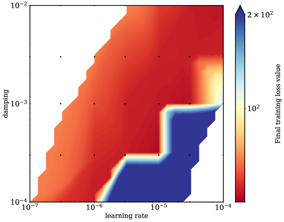
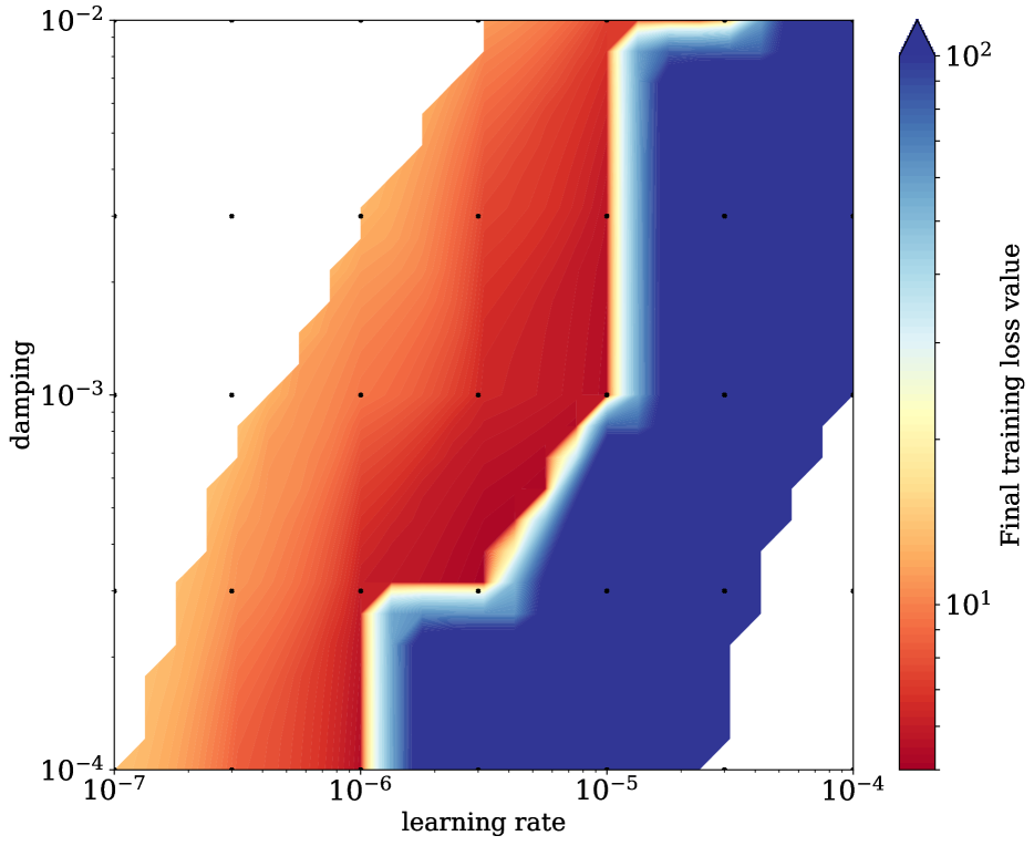
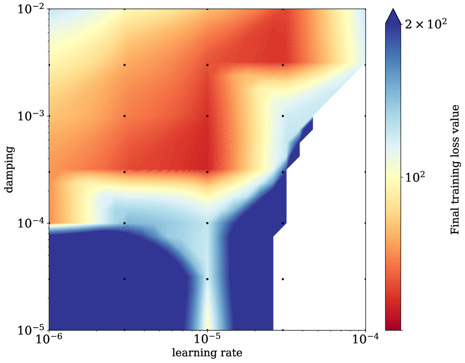
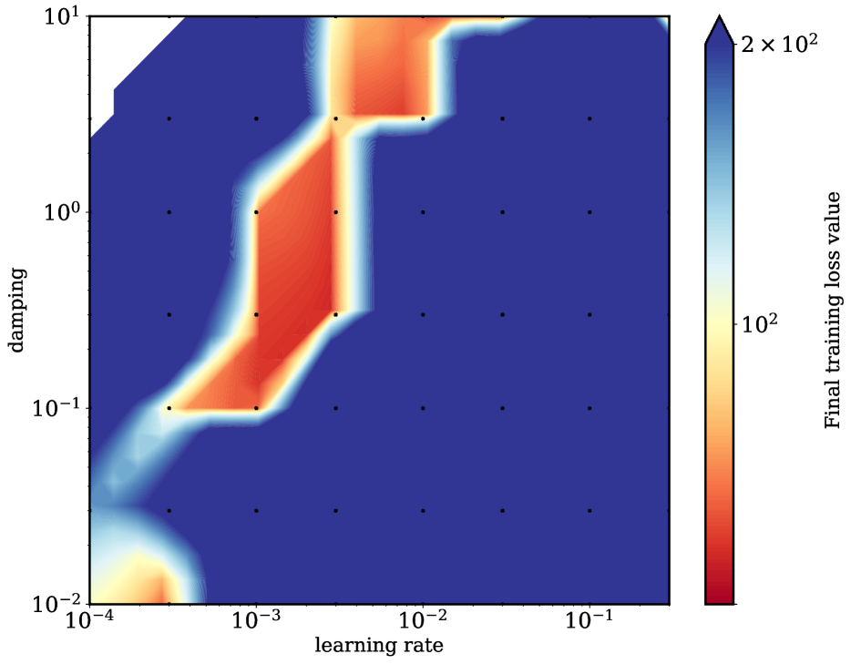
In order to obtain Figure 8, we first conducted a grid search on the learning rate (lr) and damping value based on the criteria of minimizing the training loss. The ranges of the grid searches used for the algorithms in our tests are specified in Table 5.

Table 5: Grid of hyper-parameters for autoencoder problems

Algorithm	learning rate	damping $\lambda$
SGD-m	1e-4, 3e-4, 1e-3, 3e-3, 1e-2, 3e-2	damping: not applicable
Adam	1e-5, 3e-5, 1e-4, 3e-4, 1e-3, 3e-3, 1e-2	1e-8, 1e-4, 1e-2
Shampoo	1e-5, 3e-5, 1e-4, 3e-4, 1e-3, 3e-3	1e-4, 3e-4, 1e-3, 3e-3, 1e-2
MBF	1e-7, 3e-7, 1e-6, 3e-6, 1e-5, 3e-5, 1e-4	1e-5, 3e-5, 1e-4, 3e-4, 1e-3, 3e-3, 1e-2
KFAC	1e-4, 3e-4, 1e-3, 3e-3, 1e-2, 3e-2, 1e-2, 3e-2	1e-2, 3e-2, 1e-1, 3e-1, 1e0, 3e0, 1e1

The best hyper-parameter values determined by our grid searches are listed in Table 4.

Table 6: Hyper-parameters (learning rate, damping) used to produce Figure 8

Name	MNIST	FACES	CURVES
MBF	(1e-5, 3e-4) $\to$ 51.49	(1e-6, 3e-3) $\to$ 5.17	(1e-5, 3e-4) $\to$ 55.14
KFAC	(3e-3, 3e-1) $\to$ 53.56	(1e-1, 1e1) $\to$ 5.55	(1e-2, 1e0) $\to$ 56.47
Shampoo	(3e-4, 3e-4) $\to$ 53.80	(3e-4, 3e-4) $\to$ 7.21	(1e-3, 3e-3) $\to$ 54.86
Adam	(3e-4, 1e-4) $\to$ 53.67	(1e-4, 1e-4) $\to$ 5.55	(3e-4, 1e-4) $\to$ 55.23
SGD-m	(3e-3, -) $\to$ 55.63	(1e-3, -) $\to$ 7.08	(1e-2, -) $\to$ 55.49

11.3 Experiment Settings for the CNN Problems

The ResNet32 model refers to the one in Table 6 of He et al. (2016), whereas the VGG16 model refers to model D of Simonyan & Zisserman (2014), with the modification that batch normalization layers were added after all of the convolutional layers in the model. For all algorithms, we used a batch size of 128 at every iteration.

We used weight decay for all the algorithms that we tested, which is related to, but not the same as $L_{2}$ regularization added to the loss function, and has been shown to help improve generalization performance across different optimizers Loshchilov & Hutter (2019), Zhang, Wang, Xu & Grosse (2019). The use of weight decay for MBF and Shampoo is implemented in lines 16 and 17 in Algorithm 2 and in lines 15 and 16 in Algorithm 3, respectively, and is similarly applied to SGD-m , Adam, and KFAC.

For MBF, we set $\lambda=0.003$. We also tried values around 0.003 and the results were not sensitive to the value of $\lambda$. Hence, $\lambda$ can be set to $0.003$ as a default value. For KFAC, we set the overall damping value to be 0.03, as suggested in the implementation in https://github.com/alecwangcq/KFAC-Pytorch. We also tried values around 0.03 for KFAC and confirmed that 0.03 is a good default value.

In order to obtain Figure 7, we first conducted a grid search on the initial learning rate (lr) and weight decay (wd) factor based on the criteria of maximizing the classification accuracy on the validation set. The range of the grid searches for the algorithms in our tests are specified in Table 7.

Table 7: Grid of hyper-parameters for CNN problems

Algorithm	learning rate	weight decay $\gamma$
SGD-m	3e-5, 1e-4, 3e-4, 1e-3, 3e-3, 1e-2, 3e-2, 1e-1, 3e-1, 1e0	1e-2, 3e-2, 1e-1, 3e-1, 1e0, 3e0, 1e1
Adam	1e-6, 3e-6, 1e-5, 3e-5, 1e-4, 3e-4, 1e-3, 3e-3, 1e-2, 3e-2	1e-2, 3e-2, 1e-1, 3e-1, 1e0, 3e0, 1e1
Shampoo	3e-5, 1e-4, 3e-4, 1e-3, 3e-3, 1e-2, 3e-2, 1e-1	1e-2, 3e-2, 1e-1, 3e-1, 1e0, 3e0, 1e1
MBF	1e-6, 3e-6, 1e-5, 3e-5, 1e-4, 3e-4, 1e-3, 3e-3	1e-2, 3e-2, 1e-1, 3e-1, 1e0, 3e0, 1e1
KFAC	3e-6, 1e-5, 3e-5, 1e-4, 3e-4, 1e-3, 3e-3, 1e-2, 3e-2	1e-2, 3e-2, 1e-1, 3e-1, 1e0, 3e0, 1e1

The best hyper-parameter values, and the validation classification accuracy obtained using them, are listed in Table 8.

Table 8: Hyper-parameters (initial learning rate, weight decay factor) used to produce Figure 7 and the average validation accuracy across 5 runs with different random seeds shown in Figure 7

Name	CIFAR-10 + ResNet32	CIFAR-100 + VGG16	SVHN + VGG11
MBF	(1e-4, 3e0) $\to$ 93.42%	(3e-5, 1e1) $\to$ 74.80%	(1e-3, 3e-1) $\to$ 96.59%
KFAC	(3e-3, 1e-1) $\to$ 93.02%	(1e-3, 3e-1) $\to$ 74.38%	(3e-3, 1e-1) $\to$ 96.37%
Shampoo	(1e-2, 1e-1) $\to$ 92.97%	(1e-3, 3e-1) $\to$ 73.37%	(3e-3, 1e-1) $\to$ 96.15%
Adam	(3e-3, 1e-1) $\to$ 93.34%	(3e-5, 1e1) $\to$ 72.95%	(3e-4, 1e0) $\to$ 96.34%
SGD-m	(1e-1, 1e-2) $\to$ 93.23%	(3e-2, 1e-2) $\to$ 73.99%	(3e-2, 1e-2) $\to$ 96.63%

11.4 More on MBF Implementation Motivations

11.4.1 Details on the Cosine similarity experiment

We provide in Algorithm 4 the full implementation of MBF-True for completeness. Note that, in MBF-True, the only difference with MBF is that we are using the mini-batch gradient $\overline{\mathcal{D}_{2}W_{l,b}}$ (denoted by $\mathcal{D}_{2}$ )of the model on sampled labels $y_{t}$ from the model’s distribution (see lines 10-13 in Algorithm 4) to update the estimate of mini-block preconditioners, using a moving average (lines 12, 13), with a rank one outer-product, which is different from computing the true Fisher for that mini-block.

Algorithm 4 MBF-True

0:  Given batch size $m$, learning rate $\{\eta_{k}\}_{k\geq 1}$, weight decay factor $\gamma$, damping value $\lambda$, statistics update frequency $T_{1}$, inverse update frequency $T_{2}$

1:  $\mu=0.9$, $\beta=0.9$

2:  Initialize $\widehat{G_{l,b}}=\mathbb{E}[G_{l,b}]$ ($l=1,..,k$, mini-blocks $b$) by iterating through the whole dataset, $\widehat{\mathcal{D}W_{l,b}}=0$ ($l=1,..,k$, mini-blocks $b$)

3:  for $k=1,2,\ldots$ do

4:     Sample mini-batch $M_{t}$ of size $m$

5:     Perform a forward-backward pass over $M_{t}$ to compute the mini-batch gradient $\overline{\mathcal{D}W_{l,b}}$

6:     for $l=1,...L$ do

7:        for mini-block $b$ in layer $l$, in parallel do

8:           $\widehat{\mathcal{D}W_{l,b}}=\mu\widehat{\mathcal{D}W_{l,b}}+\overline{\mathcal{D}W_{l,b}}$

9:           if $k\equiv 0\pmod{T_{1}}$ then

10:              Sample the labels $y_{t}$ from the model’s distribution

11:              Perform a backward pass over $y_{t}$ to compute the mini-batch gradients $\overline{\mathcal{D}_{2}W_{l,b}}$

12:              If Layer $l$ is convolutional: $\widehat{G_{l,j,i}}=\beta\widehat{G_{l,j,i}}+(1-\beta)\overline{\mathcal{D}_{2}W_{l,j,i}}\left(\overline{\mathcal{D}_{2}W_{l,j,i}}\right)^{\top}$

13:              If Layer $l$ is fully-connected: $\widehat{G_{l}}=\beta\widehat{G_{l}}+\frac{1-\beta}{O}\sum_{j=1}^{O}\overline{\mathcal{D}_{2}W_{l,j}}\left(\overline{\mathcal{D}_{2}W_{l,j}}\right)^{\top}$

14:           end if

15:           if $k\equiv 0\pmod{T_{2}}$ then

16:              Recompute and store $(\widehat{G_{l,b}}+\lambda I)^{-1}$

17:           end if

18:           $p_{l,b}=(\widehat{G_{l,b}}+\lambda I)^{-1}\widehat{\mathcal{D}W_{l,b}}+\gamma W_{l,b}$

19:           $W_{l,b}=W_{l,b}-\eta_{k}p_{l,b}$

20:        end for

21:     end for

22:  end for

As mentioned in the main manuscript, we explored how close MBF’s direction is to the one obtained by a block-diagonal full EFM method (that we call BDF). We provide here a detailed implementation of the procedure that we used for completeness. More specifically, for any algorithm X, we reported the cosine similarity between the direction given by X and that obtained by BDF in the procedure described in Algorithm 5.

Algorithm 5 Cosine(BDF, Algorithm X)

0:  All required parameters for Algorithm X

1:  $m=1000,\eta=0.01,\mu=0.9$, $\beta=0.9,\lambda=0.01$

2:  Initialize the block EFM matrices $\widehat{F_{l}}=\mathbb{E}[F_{l}]$ ($l=1,..,L$) by iterating through the whole dataset

3:  $\widehat{\mathcal{D}W_{l}}=0$ ($l=1,..,L$)

4:  for $k=1,2,\ldots$ do

5:     Sample mini-batch $M_{t}$ of size $m$

6:     Perform a forward-backward pass over $M_{t}$ to compute the mini-batch gradient $\overline{\mathcal{D}W_{l}}$

7:     for $l=1,...L$ do

8:        $\widehat{\mathcal{D}W_{l}}=\mu\widehat{\mathcal{D}W_{l}}+\overline{\mathcal{D}W_{l}}$

9:        $\widehat{F_{l}}=\beta\widehat{F_{l}}+(1-\beta)\mathbb{E}[F_{l}]$

10:        $p_{l}=(\widehat{F_{l}}+\lambda I)^{-1}\widehat{\mathcal{D}W_{l,b}}$

11:        Compute the direction $d_{l}$ given by algorithm X at the current iterate $W_{l}$

12:        Compute and store the cosine $\frac{|p_{l}^{T}d_{l}|}{\left\lVert p_{l}\right\rVert\left\lVert d_{l}\right\rVert}$

13:        $W_{l}=W_{l}-\eta p_{l}$

14:     end for

15:  end for

The algorithms were run on a $16\times 16$ down-scaled MNIST LeCun et al. (2010) dataset and a small feed-forward NN with layer widths 256-20-20-20-20-20-10 described in Martens & Grosse (2015). For all methods, we followed the trajectory obtained using the BDF method as described in Algorithm 5.

11.4.2 Comparison between MBF and MBF-True on Autoencoder and CNN problems

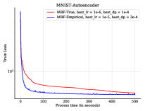
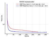
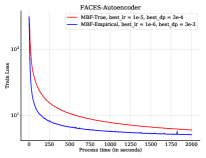
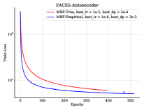
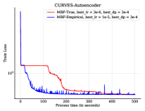
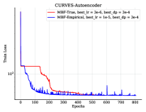
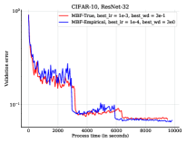
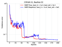
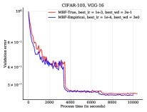
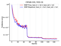
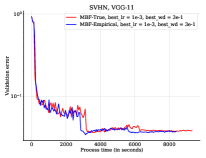
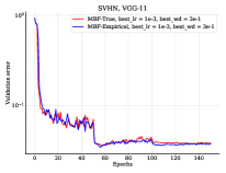
The cosine similarity results reported in the main manuscript (see Figure 6 and related discussion) on the down-scaled MNIST suggest that the direction obtained by MBF and MBF-True behave similarly with respect the direction obtained by BDF. In this section, we compare the performance of MBF-True to MBF on the same Autoencoder problems (MNIST, FACES, CURVES) described in 11.2 and the same CNN problems (CIFAR-10 + ResNet32, CIFAR-100 + VGG16, and SVHN + VGG11) described in 11.3. We used the same grid of parameters to tune MBF-True as the one described in 11.2 and 11.3. We report in Figures 9 and 10 the training and validation errors obtained on these problems, as well as the best hyper-parameters for both methods in the legends. It seems that using the symmetric outer product of the empirical mini-batch gradient to update the mini-block preconditioner yields better results than using the mini-batch gradient from sampled data from the model’s distribution to compute this inner product.

We think this might be the case because MBF is closer to being an adaptive gradient methods, which also use the empirical gradient such as ADAGRAD and ADAM, rather than a second-order natural gradient method such as KFAC, where in the latter case using a sampled gradient yields better results than using the empirical data. Note that, when the mini-block sizes are 1, MBF becomes a diagonal preconditioning method like ADAM minus the square root operation.

(a) MNIST autoencoder

(b) FACES autoencoder

(c) CURVES autoencoder

Figure 9: Training performance of MBF-True and MBF on three autoencoder problems.

(a) CIFAR-10, ResNet-32

(b) CIFAR-100, VGG-16

(c) SVHN, VGG-11

Figure 10: Testing performance of MBF-True and MBF on three CNN problems.

11.4.3 Spacial averaging on convolutional layers.

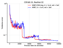
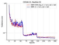
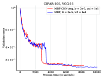
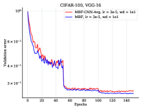
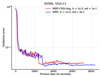
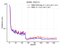
In this section, we compare the performance of MBF with spacial averaging applied to convolutional layers to MBF on the same three CNN problems (CIFAR-10 + ResNet-32, CIFAR-100 + VGG16, and SVHN + VGG11) described in 11.3. We used the same grid of parameters to tune MBF-CNN-Avg as the one described in 11.3. We report in Figure 11 the validation errors obtained on these problems, as well as the best hyper-parameters for both methods in the legends. It seems that using the average of the kernel-wise mini-blocks to update the preconditioner yields slightly worse results than using the individual mini-blocks as preconditioner. We think this might be the case because the averaging over all mini-blocks results into a loss of curvarture information as the kernel-wise mini-blocks are small in size. Note that, when using the average mini-blocks, MBF will require less memory than adaptive first order methods such as ADAM.

(a) CIFAR-10, ResNet-32

(b) CIFAR-100, VGG-16

(c) SVHN, VGG-11

Figure 11: Testing performance of MBF-CNN-Avg(MBF with spacial averaging applied to CNN layers) and MBF on three CNN problems.

11.4.4 On the effect of the update frequencies $T_{1},T_{2}$:

We also explored the effect of the update frequencies $T_{1},T_{2}$ for the mini-block preconditionners as used in Algorithm 2. To be more specific, we tuned the learning rate for various combinations of $T_{1},T_{2}$ depicted in Figure 12. Comparing the performance of Algorithm 2 for these different configurations, we can see that the effect of the frequencies $T_{1},T_{2}$ on the final performance of MBF is minimal and the configurations $T_{1},T_{2}=(1,20)$, $T_{1},T_{2}=(2,25)$ seem to yield the best performance in terms of process time for autoencoder problems.

(a) a) MNIST autoencoder, $T_{2}=10$

(b) b) MNIST autoencoder, $T_{2}=20$

(c) c) MNIST autoencoder, $T_{2}=25$

Figure 12: Training performance of MBF on MNIST autoencoder problems for some combinations of $T_{1},T_{2}$.

11.4.5 Additional inverse EMF heatmap illustrations

As mentioned in the main manuscript, we include here additional examples that illustrate that most of the weight in the inverse of the empirical Fisher matrix resides in the mini-blocks used in MBF. For convolutional layers, we trained a simple convolutional neural network, Simple CNN on Fashion MNIST (Xiao et al. 2017). The model is identical to the base model described in Shallue et al. (2019). It consists of 2 convolutional layers with max pooling with 32 and 64 filters each and $5\times 5$ filters with stride 1, “same” padding, and ReLU activation function followed by 1 fully connected layer. Max pooling uses a $2\times 2$ window with stride 2. The fully connected layer has 1024 units. It does not use batch normalization.

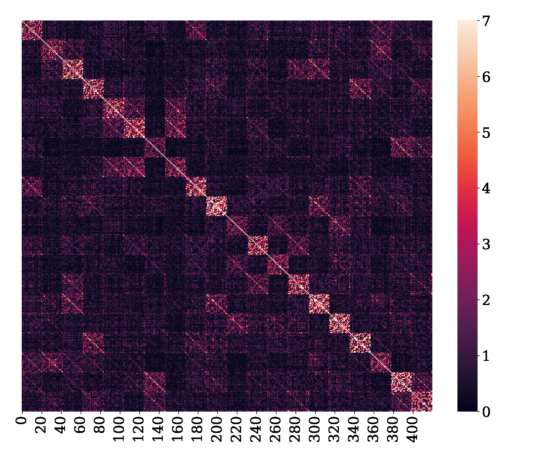
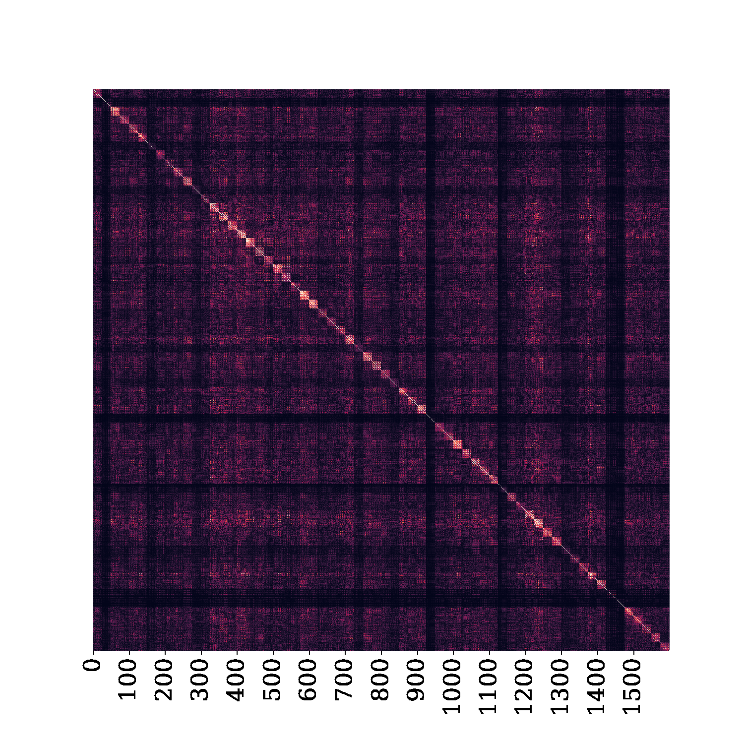
Figure 14 shows the heatmap of the absolute value of the inverse empirical Fisher corresponding to the second convolutional layer for channels 1, 16 and 32, which all use $64$ filters of size $5\times 5$ (thus 64 mini-blocks of size $25\times 25$ per channel). One can see that the mini-block (by filter) diagonal approximation is reasonable.

Figure 13: Absolute inverse EFM, second fully connected layer 20-20

(a) Absolute inverse EFM for channel 1

(b) Zoom on the 20th to 30th blocks

(c) Absolute inverse EFM for channel 16

(d) Zoom on the 20th to 30th blocks

(e) Absolute inverse EFM for channel 32

(f) Zoom on the 20th to 30th blocks

Figure 14: Absolute inverse of the empirical EFM after 10 epochs for the second convolutional layer of the Simple-CNN.

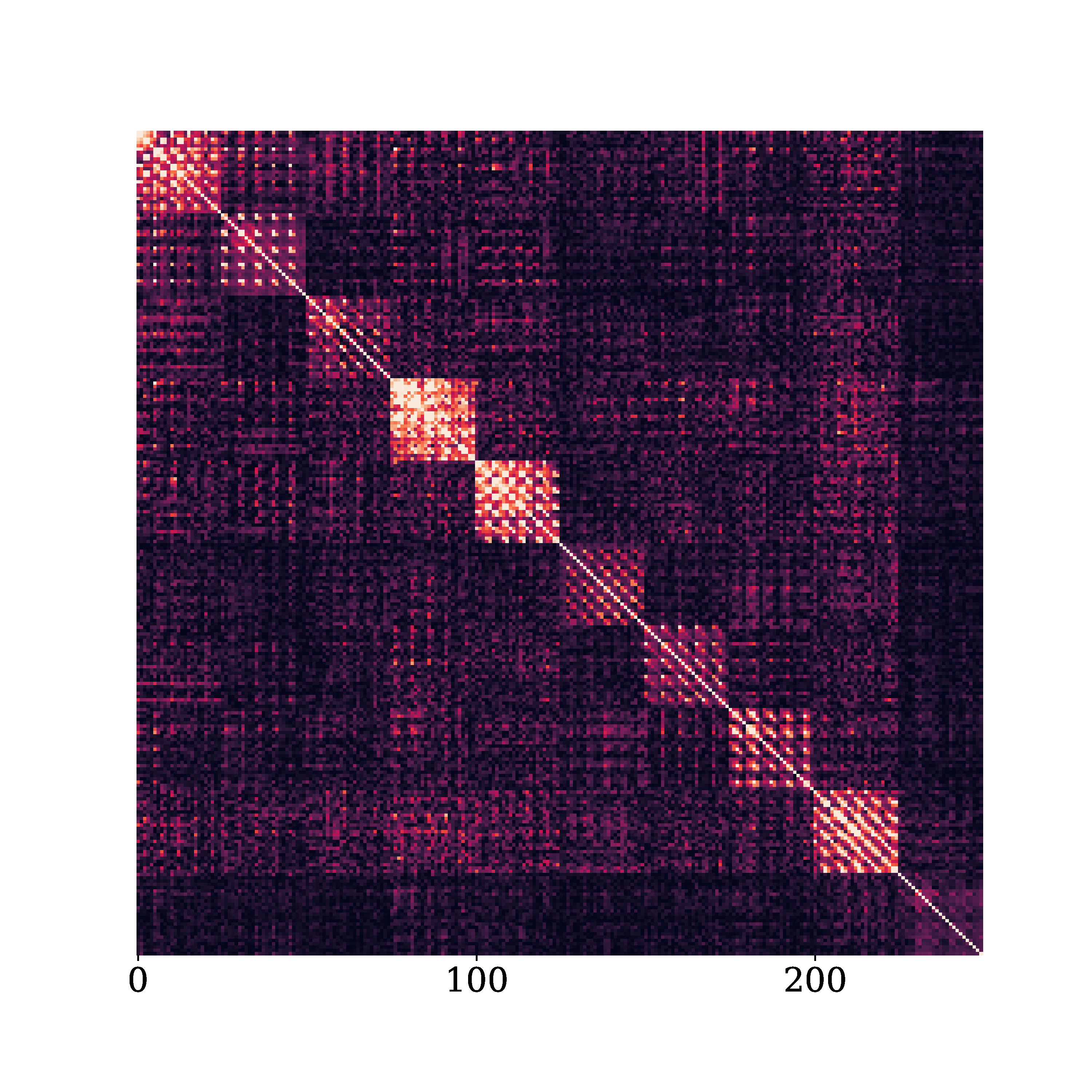
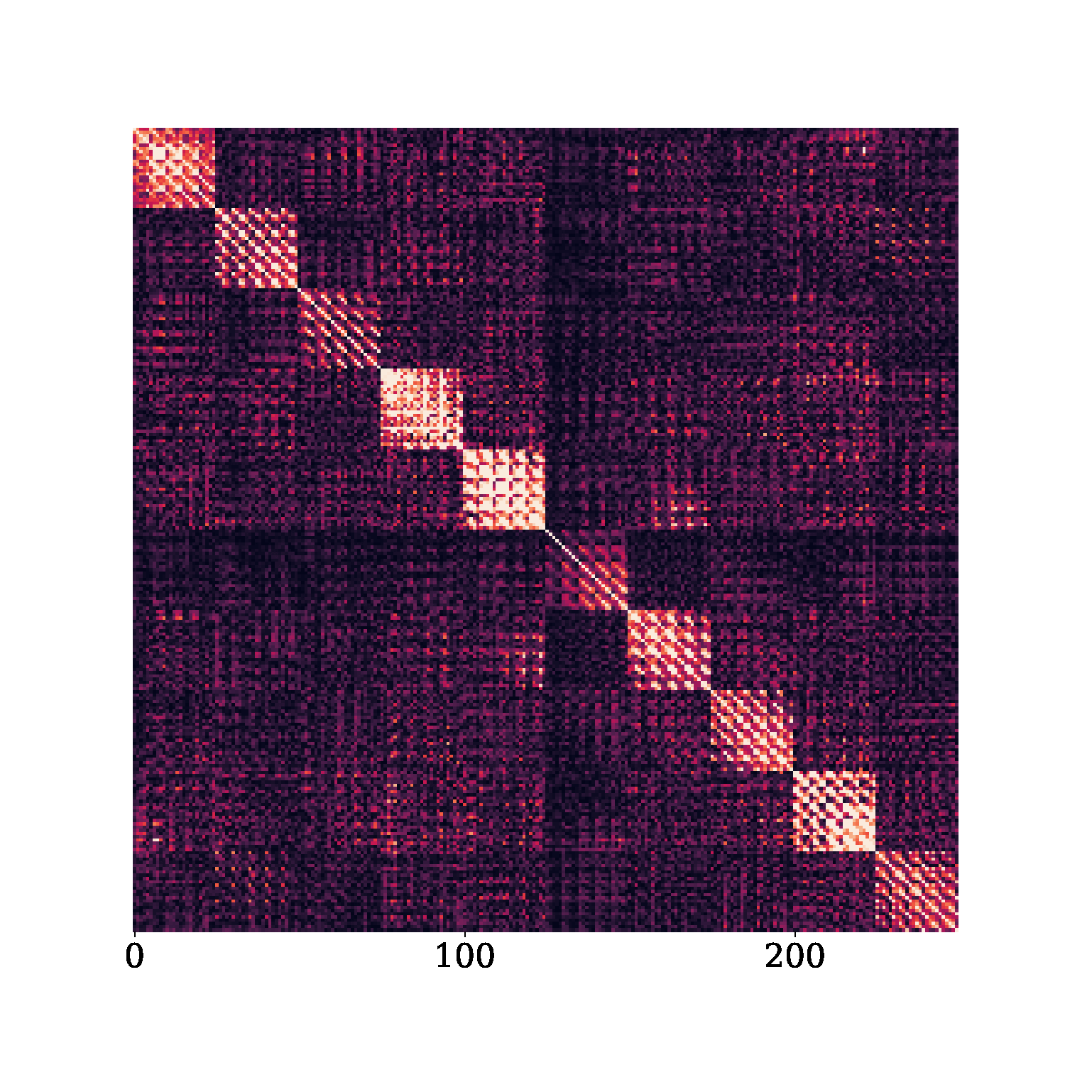
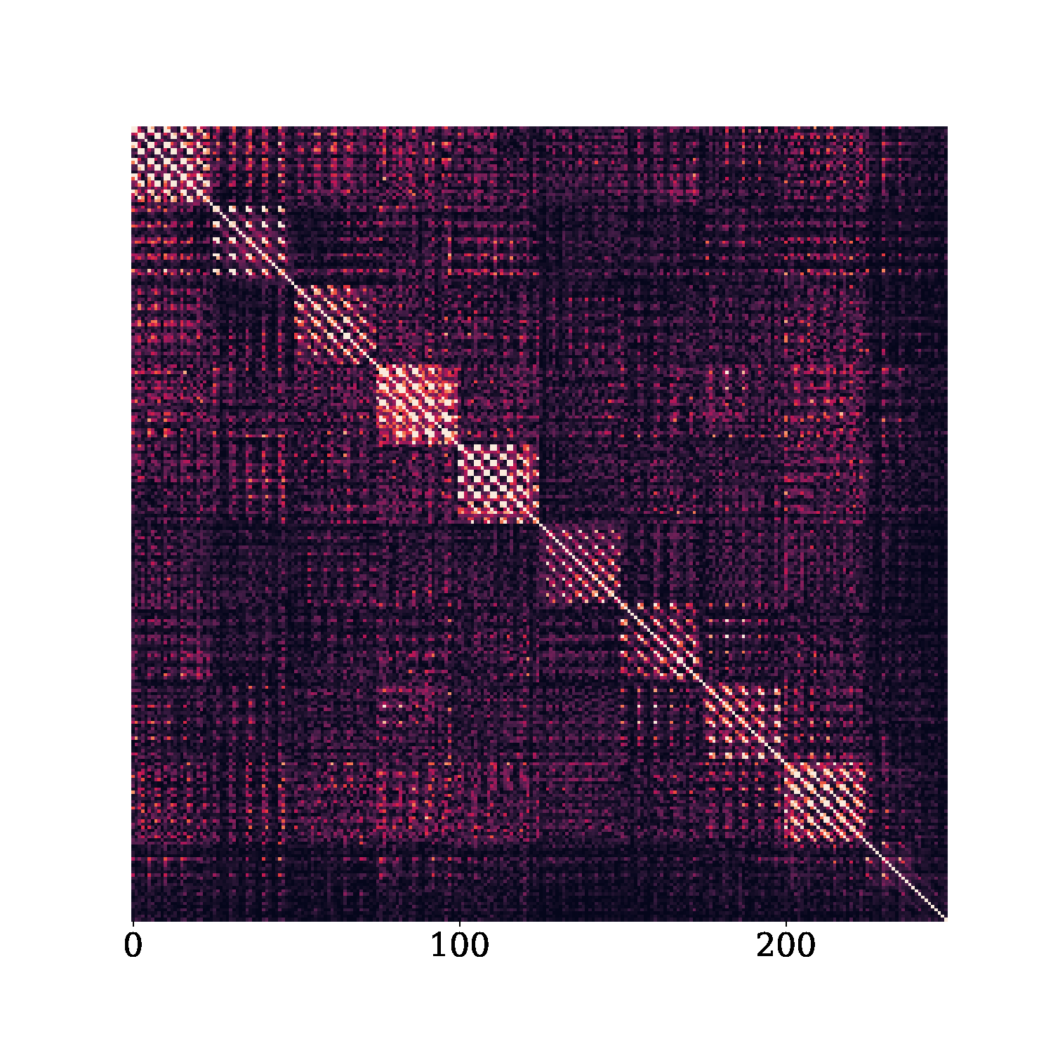
As mentioned in the manuscript, we illustrate the mini-block structure of the empirical Fisher matrix on a $7$-layer (256-20-20-20-20-20-10) feed-forward DNN using $\tanh$ activations, partially trained (after 50 epochs using SGD-m) to classify a $16\times 16$ down-scaled version of MNIST that was also used in (Martens & Grosse 2015). Figure 13 shows the heatmap of the absolute value of the inverse empirical FIM for the second fully connected layers (including bias). One can see that the mini-block (by neuron) diagonal approximation is reasonable.

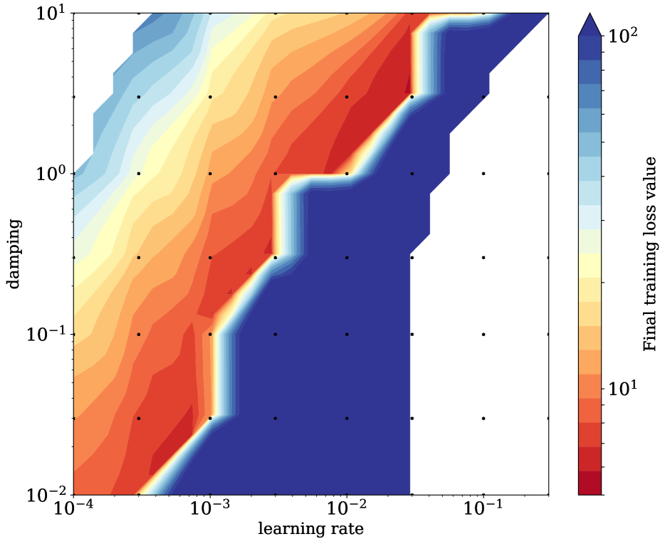
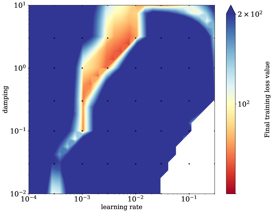
11.5 Sensitivity to Hyper-parameters:

11.6 MBF

Figure 15: Landscape of the final training loss value w.r.t hyper-parameters (i.e. learning rate and damping) for MBF. The left, middle, right columns depict results for MNIST, FACES, CURVES, which are terminated after 500, 2000, 500 seconds (CPU time), respectively.

11.7 KFAC

Figure 16: Landscape of the final training loss value w.r.t hyper-parameters (i.e. learning rate and damping) for KFAC. The left, middle, right columns depict results for MNIST, FACES, CURVES, which are terminated after 500, 2000, 500 seconds (CPU time), respectively.

11.8 Training and testing plots:

For completeness, we report in Figures 17 and 18 both training and testing performance of the results plotted in Figures 7 and 8 in the main manuscript.

(a) a) CIFAR-10, ResNet-32

(b) b) CIFAR-100, VGG16

(c) c) SVHN, VGG11

Figure 17: Training and testing performance of MBF, KFAC, Shampoo, Adam, and SGD-m on three CNN problems.

(a) MNIST autoencoder

(b) FACES autoencoder

(c) CURVES autoencoder

Figure 18: Training and testing performance of MBF, KFAC, Shampoo, Adam, and SGD-m on three autoencoder problems.

12 Limitations

We have explored using MBF in both Autoencoder and CNN problems. However, we believe it would be interesting to extend the method to other architectures such as RNNs and other sets of problems such as natural language processing (NLP) that predominately use Transformer models. It would also be interesting to extend our theoretical results to the fully stochastic case.

References

- (1)
- Amari et al. (2000) Amari, S.-I., Park, H. & Fukumizu, K. (2000), ‘Adaptive method of realizing natural gradient learning for multilayer perceptrons’, Neural computation 12(6), 1399–1409.
- Anil et al. (2021) Anil, R., Gupta, V., Koren, T., Regan, K. & Singer, Y. (2021), ‘Scalable second order optimization for deep learning’, arXiv preprint arXiv:2002.09018 .
- Botev et al. (2017) Botev, A., Ritter, H. & Barber, D. (2017), Practical gauss-newton optimisation for deep learning, in ‘International Conference on Machine Learning’, PMLR, pp. 557–565.
- Broyden (1970) Broyden, C. G. (1970), ‘The convergence of a class of double-rank minimization algorithms 1. general considerations’, IMA Journal of Applied Mathematics 6(1), 76–90.
- Byrd et al. (2016) Byrd, R. H., Hansen, S. L., Nocedal, J. & Singer, Y. (2016), ‘A stochastic quasi-newton method for large-scale optimization’, SIAM Journal on Optimization 26(2), 1008–1031.
- Choi et al. (2019) Choi, D., Shallue, C. J., Nado, Z., Lee, J., Maddison, C. J. & Dahl, G. E. (2019), ‘On empirical comparisons of optimizers for deep learning’, arXiv preprint arXiv:1910.05446 .
- Collobert (2004) Collobert, R. (2004), Large scale machine learning, Technical report, Université de Paris VI.
- Duchi et al. (2011) Duchi, J., Hazan, E. & Singer, Y. (2011), ‘Adaptive subgradient methods for online learning and stochastic optimization’, Journal of Machine Learning Research 12(Jul), 2121–2159.
- Fletcher (1970) Fletcher, R. (1970), ‘A new approach to variable metric algorithms’, The computer journal 13(3), 317–322.
- George et al. (2018) George, T., Laurent, C., Bouthillier, X., Ballas, N. & Vincent, P. (2018), ‘Fast approximate natural gradient descent in a kronecker-factored eigenbasis’, arXiv preprint arXiv:1806.03884 .
- Goldfarb (1970) Goldfarb, D. (1970), ‘A family of variable-metric methods derived by variational means’, Mathematics of computation 24(109), 23–26.
- Goldfarb et al. (2020) Goldfarb, D., Ren, Y. & Bahamou, A. (2020), Practical quasi-newton methods for training deep neural networks, in H. Larochelle, M. Ranzato, R. Hadsell, M. F. Balcan & H. Lin, eds, ‘Advances in Neural Information Processing Systems’, Vol. 33, Curran Associates, Inc., pp. 2386–2396.
- Gower et al. (2016) Gower, R., Goldfarb, D. & Richtárik, P. (2016), Stochastic block bfgs: Squeezing more curvature out of data, in ‘International Conference on Machine Learning’, pp. 1869–1878.
- Grosse & Martens (2016) Grosse, R. & Martens, J. (2016), A kronecker-factored approximate fisher matrix for convolution layers, in ‘International Conference on Machine Learning’, PMLR, pp. 573–582.
- Gupta et al. (2018) Gupta, V., Koren, T. & Singer, Y. (2018), Shampoo: Preconditioned stochastic tensor optimization, in J. Dy & A. Krause, eds, ‘Proceedings of the 35th International Conference on Machine Learning’, Vol. 80 of Proceedings of Machine Learning Research, PMLR, pp. 1842–1850.
- He et al. (2016) He, K., Zhang, X., Ren, S. & Sun, J. (2016), Deep residual learning for image recognition, in ‘Proceedings of the IEEE conference on computer vision and pattern recognition’, pp. 770–778.
- Heskes (2000) Heskes, T. (2000), ‘On "natural" learning and pruning in multilayered perceptrons’, Neural Computation 12.
- Hinton & Salakhutdinov (2006) Hinton, G. E. & Salakhutdinov, R. R. (2006), ‘Reducing the dimensionality of data with neural networks’, science 313(5786), 504–507.
- Hinton et al. (2012) Hinton, G., Srivastava, N. & Swersky, K. (2012), ‘Neural networks for machine learning lecture 6a overview of mini-batch gradient descent’, Cited on 14(8).
- ichi Amari et al. (2018) ichi Amari, S., Karakida, R. & Oizumi, M. (2018), ‘Fisher information and natural gradient learning of random deep networks’.
- Kingma & Ba (2014) Kingma, D. & Ba, J. (2014), ‘Adam: A method for stochastic optimization’, International Conference on Learning Representations .
- Krizhevsky et al. (2009) Krizhevsky, A., Hinton, G. et al. (2009), ‘Learning multiple layers of features from tiny images’.
- Krizhevsky et al. (2012) Krizhevsky, A., Sutskever, I. & Hinton, G. E. (2012), ‘Imagenet classification with deep convolutional neural networks’, Advances in neural information processing systems 25, 1097–1105.
- Kunstner et al. (2019) Kunstner, F., Hennig, P. & Balles, L. (2019), Limitations of the empirical fisher approximation for natural gradient descent, in H. Wallach, H. Larochelle, A. Beygelzimer, F. d'Alché-Buc, E. Fox & R. Garnett, eds, ‘Advances in Neural Information Processing Systems’, Vol. 32, Curran Associates, Inc.
- LeCun et al. (2010) LeCun, Y., Cortes, C. & Burges, C. (2010), ‘MNIST handwritten digit database’, ATT Labs [Online]. Available: http://yann.lecun.com/exdb/mnist 2.
- Liu & Nocedal (1989) Liu, D. C. & Nocedal, J. (1989), ‘On the limited memory bfgs method for large scale optimization’, Mathematical programming 45(1-3), 503–528.
- Loshchilov & Hutter (2019) Loshchilov, I. & Hutter, F. (2019), Decoupled weight decay regularization, in ‘International Conference on Learning Representations’.
- Martens (2010) Martens, J. (2010), Deep learning via hessian-free optimization., in ‘ICML’, Vol. 27, pp. 735–742.
- Martens (2020) Martens, J. (2020), ‘New insights and perspectives on the natural gradient method’, Journal of Machine Learning Research 21(146), 1–76.
- Martens & Grosse (2015) Martens, J. & Grosse, R. (2015), Optimizing neural networks with kronecker-factored approximate curvature, in ‘International conference on machine learning’, PMLR, pp. 2408–2417.
- Nesterov (1998) Nesterov, Y. (1998), ‘Introductory lectures on convex programming volume i: Basic course’, Lecture notes 3(4), 5.
- Ollivier (2015) Ollivier, Y. (2015), ‘Riemannian metrics for neural networks i: feedforward networks’.
- Ortega & Rheinboldt (1970) Ortega, J. & Rheinboldt, W. (1970), Iterative Solution of Nonlinear Equations in Several Variables, Classics in Applied Mathematics, Society for Industrial and Applied Mathematics (SIAM, 3600 Market Street, Floor 6, Philadelphia, PA 19104).
- Paszke et al. (2019) Paszke, A., Gross, S., Massa, F., Lerer, A., Bradbury, J., Chanan, G., Killeen, T., Lin, Z., Gimelshein, N., Antiga, L., Desmaison, A., Kopf, A., Yang, E., DeVito, Z., Raison, M., Tejani, A., Chilamkurthy, S., Steiner, B., Fang, L., Bai, J. & Chintala, S. (2019), Pytorch: An imperative style, high-performance deep learning library, in H. Wallach, H. Larochelle, A. Beygelzimer, F. d'Alché-Buc, E. Fox & R. Garnett, eds, ‘Advances in Neural Information Processing Systems 32’, Curran Associates, Inc., pp. 8024–8035.
- Polyak (1964) Polyak, B. (1964), ‘Some methods of speeding up the convergence of iteration methods’, Ussr Computational Mathematics and Mathematical Physics 4, 1–17.
- Povey et al. (2014) Povey, D., Zhang, X. & Khudanpur, S. (2014), ‘Parallel training of dnns with natural gradient and parameter averaging’, arXiv preprint arXiv:1410.7455 .
- Ren & Goldfarb (2019) Ren, Y. & Goldfarb, D. (2019), ‘Efficient subsampled gauss-newton and natural gradient methods for training neural networks’, arXiv preprint arXiv:1906.02353 .
- Ren & Goldfarb (2021a) Ren, Y. & Goldfarb, D. (2021a), ‘Kronecker-factored quasi-Newton methods for convolutional neural networks’, arXiv preprint arXiv:2102.06737 .
- Ren & Goldfarb (2021b) Ren, Y. & Goldfarb, D. (2021b), Tensor normal training for deep learning models, in A. Beygelzimer, Y. Dauphin, P. Liang & J. W. Vaughan, eds, ‘Advances in Neural Information Processing Systems’.
- Robbins & Monro (1951) Robbins, H. & Monro, S. (1951), ‘A stochastic approximation method’, The annals of mathematical statistics pp. 400–407.
- Roux et al. (2008) Roux, N., Manzagol, P.-a. & Bengio, Y. (2008), Topmoumoute online natural gradient algorithm, in J. Platt, D. Koller, Y. Singer & S. Roweis, eds, ‘Advances in Neural Information Processing Systems’, Vol. 20, Curran Associates, Inc.
- Schmidt et al. (2021) Schmidt, R. M., Schneider, F. & Hennig, P. (2021), ‘Descending through a crowded valley - benchmarking deep learning optimizers’.
- Shallue et al. (2019) Shallue, C. J., Lee, J., Antognini, J., Sohl-Dickstein, J., Frostig, R. & Dahl, G. E. (2019), ‘Measuring the effects of data parallelism on neural network training’.
- Shanno (1970) Shanno, D. F. (1970), ‘Conditioning of quasi-newton methods for function minimization’, Mathematics of computation 24(111), 647–656.
- Simonyan & Zisserman (2014) Simonyan, K. & Zisserman, A. (2014), ‘Very deep convolutional networks for large-scale image recognition’, arXiv preprint arXiv:1409.1556 .
- Soori et al. (2021) Soori, S., Can, B., Mu, B., Gürbüzbalaban, M. & Dehnavi, M. M. (2021), ‘Tengrad: Time-efficient natural gradient descent with exact fisher-block inversion’, CoRR abs/2106.03947.
- Thomas et al. (2020) Thomas, V., Pedregosa, F., van Merriënboer, B., Manzagol, P.-A., Bengio, Y. & Roux, N. L. (2020), On the interplay between noise and curvature and its effect on optimization and generalization, in S. Chiappa & R. Calandra, eds, ‘Proceedings of the Twenty Third International Conference on Artificial Intelligence and Statistics’, Vol. 108 of Proceedings of Machine Learning Research, PMLR, pp. 3503–3513.
- Vinyals & Povey (2012) Vinyals, O. & Povey, D. (2012), Krylov subspace descent for deep learning, in ‘Artificial Intelligence and Statistics’, pp. 1261–1268.
- Wang et al. (2017) Wang, M., Fang, E. X. & Liu, B. (2017), ‘Stochastic compositional gradient descent: Algorithms for minimizing compositions of expected-value functions’, Mathematical Programming 161(1-2), 419–449.
- Xiao et al. (2017) Xiao, H., Rasul, K. & Vollgraf, R. (2017), ‘Fashion-mnist: a novel image dataset for benchmarking machine learning algorithms’, arXiv preprint arXiv:1708.07747 .
- Xu et al. (2019) Xu, P., Roosta, F. & Mahoney, M. W. (2019), ‘Newton-type methods for non-convex optimization under inexact hessian information’, Mathematical Programming pp. 1–36.
- Yao et al. (2021) Yao, Z., Gholami, A., Shen, S., Keutzer, K. & Mahoney, M. W. (2021), ‘Adahessian: An adaptive second order optimizer for machine learning’, AAAI (Accepted) .
- Zhang, Martens & Grosse (2019) Zhang, G., Martens, J. & Grosse, R. (2019), ‘Fast convergence of natural gradient descent for overparameterized neural networks’, arXiv preprint arXiv:1905.10961 .
- Zhang, Wang, Xu & Grosse (2019) Zhang, G., Wang, C., Xu, B. & Grosse, R. (2019), Three mechanisms of weight decay regularization, in ‘International Conference on Learning Representations’.