Entanglement estimation in tensor network states via sampling

Abstract

We introduce a method for extracting meaningful entanglement measures of tensor network states in general dimensions. Current methods require the explicit reconstruction of the density matrix, which is highly demanding, or the contraction of replicas, which requires an effort exponential in the number of replicas and which is costly in terms of memory. In contrast, our method requires the stochastic sampling of matrix elements of the classically represented reduced states with respect to random states drawn from simple product probability measures constituting frames. Even though not corresponding to physical operations, such matrix elements are straightforward to calculate for tensor network states, and their moments provide the Rényi entropies and negativities as well as their symmetry-resolved components. We test our method on the one-dimensional critical XX chain and the two-dimensional toric code in a checkerboard geometry. Although the cost is exponential in the subsystem size, it is sufficiently moderate so that - in contrast with other approaches - accurate results can be obtained on a personal computer for relatively large subsystem sizes.

I introduction

Entanglement is the key feature of quantum mechanics that renders it different from classical theories. It takes centre stage in quantum information processing where it plays the role of a resource. The significance of notions of entanglement for capturing properties of condensed matter systems has also long been noted and appreciated Bennett et al. (1993); Horodecki et al. (2009). The observation that ground states of gapped phases of matter are expected to feature little entanglement – in fact, they feature what are called area laws for entanglement entropies Eisert et al. (2010) – is at the basis of tensor networks (TN) methods Verstraete et al. (2008); Orús (2014) accurately describing interacting quantum many-body systems. It has been noted that certain scalings of entanglement measures can indicate the presence of quantum phase transitions Osborne and Nielsen (2002); Amico et al. (2008). Indeed, the very fact that locally interacting quantum many body systems tend to be much less entangled than they could possibly be renders TN methods a powerful technique to capture their properties (Verstraete et al., 2008; Eisert et al., 2010; Eisert, 2013; Orús, 2014). Maybe most prominently, topologically ordered systems can be regarded as long ranged entangled systems Xie et al. (2019). In addition, detailed information about the scaling of entanglement properties can provide substantial diagnostic information about properties of condensed matter systems.

Accepting that tensor network states often provide an accurate and efficient classical description of interacting quantum systems, the question arises how one can meaningfully read off entanglement properties from tensor network states. This, however, constitutes a challenge. Current entanglement calculation methods in tensor network states in two and higher dimensions are highly impractical even for moderate-size systems, since they require a full reconstruction of the quantum states at heavy computational costs. For Rényi entropies one may instead employ the replica trick, which uses several copies of the RDM (as explained in Section  II.2 below); this, however, comes with an exponential scaling of the computational effort in the number of copies, often making the calculation unfeasible.

In this work, we develop a method for estimating the entanglement moments of general states represented by tensor networks. We do so by bringing together ideas of tensor network methods with those of random measurements (Merkel et al., 2010; Ohliger et al., 2013; van Enk and Beenakker, 2012; Tran et al., 2015; Elben et al., 2018; Ketterer et al., 2019; Brydges et al., 2019; Vermersch et al., 2019; Elben et al., 2020a; Cian et al., 2021; Knips et al., 2020; Joshi et al., 2020; Zhang et al., 2020) and shadow estimation Huang et al. (2020); Ohliger et al. (2013); Elben et al. (2020b); Helsen et al. (2021). In this context, it has been understood that entanglement features can be reliably estimated from expectation values of suitable random measurements.

Here, we bring these ideas to a new level by applying them to quantum states that are classically represented in the first place by tensor networks. The core idea of these methods is basically the following: While the entanglement moments naively require several copies of the system, we can refrain from this requirement by resorting to random sampling. The general protocol is to evolve the system under a random unitary drawn from the Haar measure followed by a measurement of a suitable projector. The process is repeated and moments of the results are averaged over different unitaries, giving as a result entanglement moments or other density-matrix-based properties. The effectiveness of this mindset has been demonstrated experimentally in a number of platforms, including that of cold atoms for Rényi entropies(Brydges et al., 2019; Zhang et al., 2020) and Rényi negativities(Elben et al., 2020b; Neven et al., 2021).

While these ideas have been further developed into estimation techniques Huang et al. (2020) giving rise to classical representations in their own right, we turn these ideas upside down by applying them to quantum systems that are already classically represented by tensor networks. There are some crucial differences that arise in classical representations compared to quantum experiments: First, they are much more suitable for a direct calculation of expectation values, rather than estimating them from sampling from measurements. Second, and importantly, when performing a classical simulation, we are not limited to physically-allowed actions, and specifically, we are not constrained to the application of unitary operators and measurements. This feature is to an extent reminiscent of shadow estimation in that also there, unphysical maps are made use of. It is the estimation procedure itself that is not physical here, however. The method we develop allows for having only a single copy of the simulated state, and at the same time for estimating the entanglement moments based on matrix elements that are naturally calculated. Instead of sampling operators from the Haar measure or some unitary $n$-design Gross et al. (2007), we only need to sample from a simple, finite set of tensor products of independent $d$-dimensional vectors – specifically from what are called frames or spherical complex 1-designs Renes (2004), where $d$ is the Hilbert space of a single site in the system. Furthermore, this simple structure allows our method to be applied to arbitrary system geometries.

The remainder of this work is organized as follows. Section II includes preliminary theoretical background. The Rényi moments we aim to estimate are defined and their relation to standard entanglement measures is discussed in Section II.1. Section II.2 covers the basic ideas of the TN ansatzes we use in our work: For one-dimensional systems, the matrix product state (MPS) ansatz, and in higher dimensions, projected-entangled-paired-states (PEPS) and its infinite system size version known as iPEPS. We discuss the algorithms we used for extracting the reduced density matrix and the naive method for estimating entanglement moments of states represented by these ansatzes. The solvable models used as benchmarks for testing our method are presented in Section II.4. In Section III we explain our proposed algorithm for using random variables for estimating the entanglement moments of TN in general dimension, and study the variance of the estimate in Section IV.2, from which arises the complexity of an estimation up to a chosen error. We benchmark the algorithm with the ground states of the exactly solvable toric code model, Eq. (13), using iPEPS, and the XX chain, Eq. (16), using MPS, in Section IV. Finally, we discuss the results and future steps in the conclusions, Section V. In the appendix, we present variance estimations of the Rényi moments in the general case (Appendix A), as well as specifically in the toric code model, which is used as a benchmark (Appendix B).

II Preliminaries

II.1 Entanglement measures

For a quantum system in a pure state $\rho=\ket{\psi}\bra{\psi}$, we define for a subsystem the reduced quantum state or reduced density matrix (RDM) as

$$\rho_{A}:=\mathrm{Tr}_{\overline{A}}(\rho).$$ (1)

The entanglement of the subsystem $A$ with its environment (consitutung its complement) $\overline{A}$ is encoded in the RDM. We introduce the moments of the RDM. For a positive integer $n$, the $n$-th RDM moment is defined to be

$$p_{n}(\rho_{A}):=\mathrm{Tr}(\rho_{A}^{n}),$$ (2)

also referred to as the Rényi moments. On top of being entanglement monotones (Wilde, 2016) and hence measures of entanglement in their own right, these moments are used for defining various entanglement measures with useful mathematical properties (Bennett et al., 1996; Hill and Wootters, 1997; Życzkowski et al., 1998; Rungta et al., 2001; Horodecki, 2001; Vidal and Werner, 2002; Kim, 2010; Yang et al., 2021). The RDM moments can – under mild mathematical conditions – be analytically continued to the entanglement measure featuring the strongest interpretation for pure bi-partite quantum states, the von Neumann entanglement entropy(Von Neumann, 1932) defined as

$$S(\rho_{A}):=-\mathrm{Tr}\left(\rho_{A}\log\rho_{A}\right)$$ (3)

for RDMs $\rho_{A}$, as the $1$-Rényi entropy. The von Neumann entropy is obtained in the limit $S(\rho_{A})=\lim_{n\rightarrow 1}(1-n)^{-1}\log\left(p_{n}(\rho_{A})\right)$. The Rényi moments are especially popular as entanglement indicators since they do not require a full reconstruction of the RDM spectrum. Therefore, they are often easier to either calculate theoretically or measure experimentally than other entanglement measures(van Enk and Beenakker, 2012; Daley et al., 2012; Tran et al., 2015; Islam et al., 2015; Pichler et al., 2016; Brydges et al., 2019; Elben et al., 2018; Cornfeld et al., 2019a; Zhang et al., 2020; Knips et al., 2020).

The measures above are appropriate when quantifying the entanglement between a subsystem $A$ and its environment $\overline{A}$ when $A\cup\overline{A}$ is in a pure state. When characterizing the entanglement between two subsystems $A_{1}$ and $A_{2}$ whose union $A$ is not necessarily pure, the quantities above will no longer be suitable to quantify entanglement, as they cannot distinguish between the quantum entanglement between $A_{1}$ and $A_{2}$ from their entanglement with the environment. One of the best known measures for the entanglement between two subsystems labeled as $A_{1}$ and $A_{2}$ is the entanglement negativity Eisert and Plenio (1999); Eisert (2001); Vidal and Werner (2002), based on the positive partial transpose (PPT) criterion(Peres, 1996; Hor, 1996; Horodecki et al., 2009)

$$\mathcal{N}(\rho_{A}):=\frac{\|\rho_{A}^{T_{2}}\|_{1}-1}{2},$$ (4)

where $\|\cdot\|_{1}$ denotes the trace norm, and $\rho_{A}^{T_{2}}$ the partial transposition of the degrees of freedom corresponding to $A_{2}$ in $\rho_{A}$,

$$\bra{i}_{A_{1}}\bra{j}_{A_{2}}\rho_{A}\ket{k}_{A_{1}}\ket{l}_{A_{2}}=\bra{i}_{A_{1}}\bra{l}_{A_{2}}\rho_{A}^{T_{2}}\ket{k}_{A_{1}}\ket{j}_{A_{2}},$$

for all vectors $(\ket{i},\ket{k}),(\ket{j},\ket{l})$ in an orthonormal basis of the Hilbert spaces of $A_{1},A_{2}$, respectively. The usefulness of the negativity as an entanglement measure for two subsystems in a mixed state Eisert (2001); Vidal and Werner (2002) leads us to define the moments of the partially-traced RDM, further referred to as PT moments. The $n$-th PT moment is defined to be

$$R_{n}(\rho_{A}):=\mathrm{Tr}\text{$\left((\rho_{A}^{T_{2}})^{n}\right)$}$$ (5)

for a positive integer $n$. The negativity can be obtained by an analytic continuation of the PT even integer moments by $\|\rho_{A}^{T_{2}}\|_{1}=\lim_{n\rightarrow 1/2}R_{2n}(\rho_{A})$. The PT moments are not entanglement monotones, but they can be used to detect entanglement between $A_{1}$ and $A_{2}$(Elben et al., 2020b; Neven et al., 2021), as well as for estimating the negativity(Gray et al., 2018). The popularity of the PT moments as entanglement indicators stems from the fact that they too do not require a full reconstruction of the partially transposed RDM, and are therefore easier to calculate and measure experimentally(Cornfeld et al., 2019a; Elben et al., 2020b).

For systems with a conserved charge $Q$, the quantum state of the full system typically commutes with the charge operator,

$$[\rho,\hat{Q}]=0.$$ (6)

A partial trace can be applied to the permutation relation above to give $[\rho_{A},\hat{Q}_{A}]=0$, where $\hat{Q}_{A}$ is the charge operator on subsystem $A$. The RDM is thus composed of blocks, each corresponding to a charge value $q$ in subsystem $A$, as illustrated in the inset of Fig. 6. We denote the RDM block corresponding to charge $q$ by $\rho_{A}(q)$. The entanglement measures, and specifically the RDM moments, can then be decomposed into suitable contributions from the different blocks called charge-resolved or symmetry-resolved moments(Laflorencie and Rachel, 2014; Goldstein and Sela, 2018; Xavier et al., 2018; Barghathi et al., 2018),

$$p_{n}(\rho_{A},q):=\mathrm{Tr}\left(\rho_{A}(q)^{n}\right),$$ (7)

again for positive integers $n$. This definition could be extended to the negativity as well(Cornfeld et al., 2018). The study of symmetry-resolved entanglement has drawn much interest lately, both analytically and numerically(Cornfeld et al., 2019b; Feldman and Goldstein, 2019; Fraenkel and Goldstein, 2020; Murciano et al., 2020; Capizzi et al., 2020; Parez et al., 2021; Tan and Ryu, 2020; Fuji and Ashida, 2020; Azses et al., 2020; Azses and Sela, 2020; Estienne et al., 2021; Zhao et al., 2021; Vitale et al., 2021; Neven et al., 2021; Fraenkel and Goldstein, 2021) as well as in the development of experimental measurement protocols(Goldstein and Sela, 2018; Cornfeld et al., 2018; Lukin et al., 2019; Cornfeld et al., 2019a). It reveals the relation between entanglement and charge and can point to effects such as topological phase transitions(Cornfeld et al., 2019b; Fraenkel and Goldstein, 2020; Azses et al., 2020) or to instances of dissipation in open systems dynamics(Vitale et al., 2021).

The estimation of symmetry-resolved entanglement can be done based on the analysis in Ref. Goldstein and Sela, 2018: We introduce the so-called flux-resolved RDM moments as

$$p_{n}(\rho_{A},\varphi):=\mathrm{Tr}\left(e^{i\varphi\hat{Q}_{A}}\rho_{A}^{n}\right),$$ (8)

where $\varphi\in[0,2\pi)$ can be thought of as an Aharonov-Bohm flux inserted in the replica trick. The symmetry-resolved moments can be extracted from the flux-resolved moments by a Fourier transform according to

$$p_{n}(\rho_{A},q):=\frac{1}{N_{A}}\sum_{\varphi}p_{n}(\rho_{A},\varphi)e^{-iq\varphi},$$ (9)

where $\varphi=2\pi k/N_{A}$ and $k=0,\dots,N_{A}-1$.

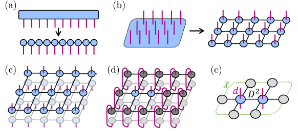
Figure 1: (a-b) A general pure quantum state can be thought of as a rank $N$ tensor represented by a single tensor with $N$ legs (indices), each with degree $d$. The full tensor capturing the entire quantum state can be decomposed into $N$ tensors, each representing a single site. The legs of the original tensor (in pink) are now divided between all tensors, and will be referred to as the physical index. Each tensor has additional legs connecting it to its neighbours, which will be referred to as the bond index. Contracting all the bond indices will result in the original tensor. (a) and (b) represent states in a one and two spatial dimensions, respectively. (c) Representing the density matrix of a pure state by taking two copies and applying complex conjugation to one of them, which is indicated by the physical index facing downwards. (d) The RDM of the sites in blue is obtained by tracing out the degrees of freedom of the sites in grey, which in turn is obtained by contracting the physical legs of both copies. (e) The RDM can be represented by the site tensors of the sites in $A$ from both copies, which is here represented by a single tensor with two physical legs, and boundary tensors, which have only bond indices. In order to obtain the boundary tensors, we use the boundary MPS method(Jordan et al., 2008a). The dimension of the bond indices in black is $D^{2}$, while that of the legs in green, connecting the boundary tensors to each other, is $\chi$, the bond dimension of the environment.

II.2 Tensor networks

We will now briefly review the TN tools that are being used to compute the quantities presented above in the remainder of this work by means of sampling techniques.

II.2.1 Matrix product states

We here consider a one-dimensional spin system, so of a finite local dimension, featuring $N$ lattice sites. The state vector of the system can be written as

$$\ket{\psi}=\sum_{\sigma_{1},\dots,\sigma_{N}}\Psi_{\sigma_{1},\dots,\sigma_{N}}\ket{\sigma_{1},\dots,\sigma_{N}},$$ (10)

where $\Psi$ is the rank $N$ tensor of the coefficients of $\ket{\psi}$. $\Psi$ has $d^{N}$ complex amplitudes, where $d$ is the Hilbert space size of a single spin. In an MPS representation we decompose $\Psi$ into $N$ different tensors, each corresponding to a single site, as illustrated in Fig. 1a. Each such tensor will have a single index corresponding to the indices of the original tensor, often called the ‘physical leg’ or the ‘physical index’, and two additional indices connecting with the tensors corresponding to the site’s neighbours, often called ‘entanglement legs’ or ‘bond indices’ (with only one bond index for the sites at the edges). Contracting all the bond indices will result in the original tensor $\Psi$. In many cases one can limit the dimension of the bond index to be some chosen constant $D$, also known as the bond dimension, and discard the least significant variables. In this way, the number of real parameters will be scaling as $O(ND^{2}d)$, at the cost of getting an approximate representation for the state. States that are expected to be well approximated by such limited tensors obey an entanglement area-law(Verstraete et al., 2008; Eisert et al., 2010; Eisert, 2013; Orús, 2014) (in fact, this is provably the case for area laws of suitable Rényi entropies Schuch et al. (2008)). This MPS decomposition is a widely used method for the simulation of ground states(White, 1992; Vidal, 2004), thermal states(Verstraete et al., 2004; Zwolak and Vidal, 2004; Weimer et al., 2021) and states undergoing a time evolution(Vidal, 2003; White and Feiguin, 2004; Orús and Vidal, 2008; Paeckel et al., 2019) generated by local Hamiltonians of one-dimensional systems.

For a system partitioned into two contiguous subsystems, the extraction of the spectrum of the RDM, also called the entanglement spectrum, is very naturalSchollwöck, 2011 and can often be useful in classifying phases of matter in one spatial dimension(Pollmann et al., 2010; Schuch et al., 2011; Pollmann et al., 2012; Kshetrimayum et al., 2015). We note that a decomposition of the system into two tensors, one corresponding to subsystem $A$ and one to $\overline{A}$, is built into the decomposition of the systems into site tensors, and that this decomposition can be transformed into the Schmidt decomposition of the state vector

$$\ket{\psi}=\sum_{i}\psi_{i}\ket{i}_{A}\ket{i}_{\overline{A}},$$ (11)

where $\{\ket{i}_{A}\},\{\ket{i}_{\overline{A}}\}$ are orthonormal bases of $A,\overline{A}$, respectively. The values $\{\psi_{i}\}$ are called the Schmidt values, and can be extracted by a singular value decompositionSchollwöck, 2011. The RDM is thus

$$\rho_{A}=\sum_{i}|\psi_{i}|^{2}\ket{i}_{A}\bra{i}_{A}.$$ (12)

The RDM eigenvalues are thus the squared absolute values of the Schmidt values, and by obtaining them, we can extract the RDM moment in all ranks $n$, as well as the von Neumann entropy. Specific techniques have been developed for the extraction of entanglement measures in some additional cases, such as the entanglement of a contiguous subsystem of an infinite system(Cirac et al., 2020) or the negativity of two contiguous subsystems(Ruggiero et al., 2016).

II.2.2 Projected entangled pair states

For two or higher dimensional lattice systems, the MPS formalism is extended to an ansatz called projected entangled pair states (PEPS)Verstraete and Cirac, 2004; Jordan et al., 2008b. The tensor capturing the state vector of the entire lattice is then decomposed into $N$ site tensors, each with a single physical index and a bond index for each neighbour of the site in the system. An example for a square lattice is depicted in Fig. 1b, and the generalization to other lattice configurations is straightforward.

The infinite version of PEPS, known as iPEPS(Jordan et al., 2008b), can be used to represent states in the thermodynamic limit in 2D. They are defined by a finite set of tensors repeated all over the lattice with some periodicity. iPEPS have found numerous applications in studying ground states(Corboz, 2016; Liao et al., 2017; Picot et al., 2016; Kshetrimayum et al., 2016, 2020a; Boos et al., 2019), thermal states(Czarnik et al., 2012; Kshetrimayum et al., 2019; Mondal et al., 2020) and non-equilibrium problems(Kshetrimayum et al., 2017; Czarnik et al., 2019; Hubig and Cirac, 2019; Kshetrimayum et al., 2020b, 2021; Dziarmaga, 2021) in two spatial dimensions, and have become state of the art numerical technique for studying strongly correlated two-dimensional problems. The technique does not suffer from the infamous sign problem(Barthel et al., 2009; Corboz et al., 2010) and can go to very large system sizes, thus allowing access to regimes where techniques like Quantum Monte Carlo and exact diagonalization fail.

The pure quantum state $\rho=\ket{\psi}\bra{\psi}$ of the quantum system can be obtained by taking a PEPS state vector and its Hermitian conjugate and placing them back to back as a tensor product, as depicted for PEPS in Fig. 1c. We now examine a rectangular subsystem $A$ with $N_{A}=w_{1}\times w_{2}$ sites, where $w_{1}\leq w_{2}$ (as will be the notation throughout this work). In order to get the RDM of $A$ as defined in Eq. (1), the degrees of freedom of $\overline{A}$ need to be traced out. This can be obtained by contracting the physical legs of all tensors corresponding to sites in $\overline{A}$ with the physical legs of the same tensor in the complex conjugate. We get a RDM composed of site tensors for the tensors in $A$, and boundary tensors resulting from the tensors in $\overline{A}$, as depicted in Fig. 1e. Such boundary tensors can be approximately computed for an infinite system. We remark here that exactly contracting PEPS tensors is a computationally hard problem (in worst case complexity and for meaningful probability measures even in average case)(Schuch et al., 2007; Haferkamp et al., 2020a) and therefore, we have to rely on approximation algorithms such as the corner transfer matrix renormalization group algorithm(Nishino and Okunishi, 1996; Orús and Vidal, 2009) boundary MPS techniques(Jordan et al., 2008a), higher order tensor renormalization group methods(Xie et al., 2012) or others. It is also known that those PEPS that are ground states of uniformly gapped parent Hamiltonians – which are interesting in the condensed matter context – can actually be contracted in quasi-polynomial time Schwarz et al. (2017). In this work, we make use of the boundary MPS technique: We create a one-dimensional TN representing the boundary of the (supposedly infinite) system, and multiply it by the ‘traced out’ tensors indicated in Fig. 1d. The boundary bond dimension is limited to a constant dimension $\chi$. This process is then repeated until the one-dimensional boundary tensors are converged, resulting in a one-dimensional boundary as depicted in Fig. 1e.

II.3 Entanglement measures computed from reduced states

The entanglement measures presented in Section II.1 can be extracted for two contiguous systems in an MPS as presented in Section II.2.1, as well as in additional specific cases in one(Ruggiero et al., 2016; Cirac et al., 2020) and two(Orús et al., 2014) spatial dimensions. However, for a general dimension and partition, there is no efficient way known to quantify the entanglement. A straightforward method can be contracting the tensors such that the RDM is obtained explicitly to then obtain its spectral decomposition. However, the explicit RDM is of dimension $d^{N_{A}}\times d^{N_{A}}$, which comes along with substantial computational effort and which imposes a strong restriction on the accessible system sizes.

That being said, the $n$-th RDM or PT moments defined in Eqs. (2, 5) can be calculated in polynomial time in $N_{A}$ using $n$ copies of the system tensors as depicted in Fig. 2 for a two-dimensional PEPS. The space complexity required for performing this multiplication for an MPS scales as $O\left(d^{2n}D^{2n}+D^{4n}\right)$. The space complexity for a two-dimensional PEPS is given by $O\left(\chi^{2n}D^{2(w_{1}+1)n}+D^{8n}d\right)$, where $\chi$ is the bond dimension of the environment as depicted in Fig. 1e, and $w_{1}$ is the short edge of the rectangular system, as define in Section II.2.2 above. For $n>1$, the exponential dependence of the cost on $n$ quickly makes it prohibitively large, despite the fact that for a narrow system (constant $w_{1}$), the time complexity is linear in $N_{A}$ and the space complexity does not depend on $N_{A}$ (except for the possible dependence of $D$ on $N_{A}$, as can sometimes happen in finite systems).

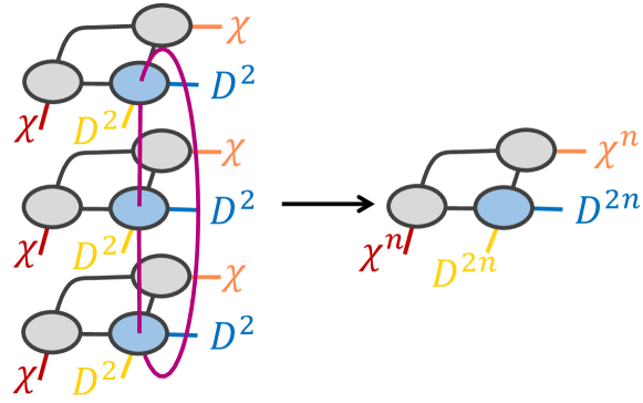
Figure 2: Contracting $n$ copies of the density matrix (here $n=3$) to get the $n$-th RDM moment can be done site by site as in the figure. The exponential dependence of the dimension of $\rho_{A}$ on $N_{A}$ turns into a linear dependence. However, a prohibitive exponential dependence on $n$ emerges instead.

II.4 Benchmark models

Before turning to presenting the actual sampling method for computing entanglement measures in quantum systems captured by tensor networks, we here first present the models we used for benchmarking our method: The two-dimensional gapped toric code model on a square lattice and the one-dimensional gapless XX model.

II.4.1 The toric code model

The first benchmark model we elaborate on is the analytically solvable toric code model on a square lattice. The toric code, introduced by Kitaev(Kitaev, 2003), transferring insights from topological quantum field theory to the realm of quantum spin systems, is a model of spins on a square lattice with local dimension $d=2$. The spins live on the edges of the lattice rather than its nodes. The Hamiltonian of the model is given by

$$H=-J_{s}\sum_{s}\otimes_{i\in s}\sigma_{i}^{x}-J_{p}\sum_{p}\otimes_{i\in p}\sigma_{i}^{z}.$$ (13)

$s$ in the equation above represents the set of edges around a single node in the lattice (a star) and $p$ represents the set of edges forming a plaquette in the lattice, as shown in Fig. 3. The ground state of toric code model displays several important properties, among which are topological order, which leads to robustness to local errors, making it an important candidate for fault-tolerant error correction code. For $J_{s},J_{p}>0$, the ground state vector of the model with open boundary conditions is known and can be written as

$$\ket{\psi_{0}}=\prod_{s}\frac{(\mathbb{I}+\otimes_{i\in s}\sigma_{i}^{x})}{2}\ket{0}^{\otimes N},$$ (14)

where $N$ is the number of all sites in the system. In the limit $N\rightarrow\infty$, the iPEPS representation of the infinite toric code ground state is given in Refs. Verstraete et al., 2006; Orús, 2014. A set of two site tensors, $T_{A}$ and $T_{B}$, are repeated infinitely such that all of the nearest-neighbours of a site represented by $T_{A}$ are of the form $T_{B}$ and vice versa. The bond dimension of all bond indices of $T_{A}$ and $T_{B}$ is $D=2$.

For a subsystem of the infinite system in the state defined in Eq. (14), the density-matrix-based measures can be analytically calculated(Hamma et al., 2005). This relies on the symmetry of the ground state under the application of $\otimes_{i\in s}\sigma_{i}^{x}$ for all stars $s$ and of $\otimes_{i\in p}\sigma_{i}^{z}$ for all plaquettes $p$. Due to this symmetry, the RDM is block diagonal, where the size of each block equals the order of the group generated by each operator, which is 2 for the operators above. Considering the fact that all non-zero blocks are identical, as can be seen from Eq. (14), the eigenvalues of the RDM can be extracted analytically. Note that the symmetry mentioned above is not utilized in the numerical method, so as to make our performance results applicable to general analytically-unsolvable models, which do not posses such local symmetries. Here, we estimate the 2nd, 3rd and 4th RDM moments, as well as the 3rd PT moment, for a checkerboard-like partition of a square subsystem ($w_{1}=w_{2}=w$), as shown for $w=6$ in Fig. 3. We study the cases of $w=4,6,8$. Note that while the toric code displays an area law type entanglement structure, here the entire system is in the area and therefore a volume law is reached. Such extensive partitions were shown to be interesting for the study of topological phases in Refs. (Hsieh and Fu, 2014; Vijay and Fu, 2015) and following works (a more traditional geometry is studied in Appendix B). For such systems, the $n$-th RDM moment is shown to be(Hamma et al., 2005)

$$p_{n}(\rho_{A})=R_{n}(\rho_{A})=2^{-(w^{2}/2-1)(n-1)}.$$ (15)

The log of the moment deviates from an area law by an additive constant term, reflecting the the topological order of the model(Kitaev and Preskill, 2006; Levin and Wen, 2006). Note that for the toric code ground state $p_{3}=R_{3}$ due to the structure of the RDM discussed above. However, we compute an estimate for $R_{3}$ based on the generally-applicable estimator defined in Eq. (25) for completeness.

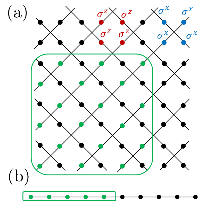
Figure 3: (a) The toric code model on a square lattice. In blue is an example of a star operator, $\otimes_{i\in s}\sigma_{i}^{x}$, and in red an example of a plaquette operator, $\otimes_{i\in p}\sigma_{i}^{z}$. Circled in green is an example subsystem of dimensions $w=6$, where the system is composed of the sites colored in green. (b) The XX model is defined on a finite one-dimensional chain, where subsystem $A$ is its left half as circled and colored in green.

II.4.2 The XX model

While suited for high dimensions, we note that our method is blind to the dimensionality of the system, and will apply to one-dimensional systems in precisely the same way as it would for higher dimensions. Therefore, we can use one-dimensional models as benchmark models for testing the system. We test our model on the ground state of the one-dimensional XX model captured by the local Hamiltonian

$$H=J\sum_{i}\sigma_{i}^{+}\sigma_{i+1}^{-}+\mathrm{h.c.,}$$ (16)

where $i$ stands for a site in the system. The Hamiltonian can be seen as a Hamiltonian of non-interacting fermions by virtue of the Jordan-Wigner transformation(Jordan and Wigner, 1928) and is thus analytically solvable(Peschel, 2003). We compute the ground state of a system of length $2l$ and extract the 2nd, 3rd and 4th RDM moments of a contiguous half of the system. In contrast to the toric code, the XX model is gapless in the absence of a large magnetic field and can be well approximated as a conformal system. For such systems, the RDM moments of a subsystem when the total system is in the ground state is to a good approximation predicted to be (Calabrese and Cardy, 2009; Jin and Korepin, 2004),

$$p_{n}(\rho_{A})\sim\frac{1+n^{-1}}{6}N_{A}^{-c(n-1/n)/6},$$ (17)

where $c=1$ is the conformal charge. As opposed to the toric code ground state RDM, which is composed of $2\times 2$ blocks, the XX ground state is not as structured, and the performance of the method is harder to predict. As such, the XX model ground state is a good complement to the toric code ground state in the study of the method’s performance.

III Method

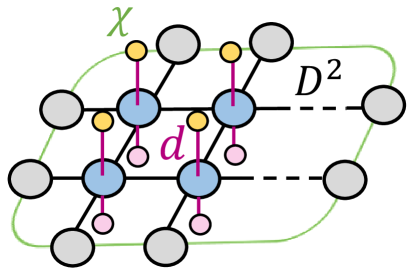
Figure 4: Graphical representation of the computation of a single element $\bra{V^{(i)}}\rho\ket{V^{(j)}}$ on an iPEPS. The system in the figure is a rectangle system of height $h=2$ (and a general width $w$). The local vectors $\ket{v^{[\alpha]}}$ are represented by the yellow and pink one-legged circles, where the two sets of local vectors are independent of each other.

We now turn to describing the method that is at the heart of this work. The core idea is that with suitable stochastic sampling techniques, one can more resource-efficiently estimate entanglement properties of systems captured by tensor networks. Inspired by the growing body of methods based on random unitaries, (Merkel et al., 2010; van Enk and Beenakker, 2012; Ohliger et al., 2013; Tran et al., 2015; Elben et al., 2018; Ketterer et al., 2019; Brydges et al., 2019; Vermersch et al., 2019; Elben et al., 2020a; Cian et al., 2021; Knips et al., 2020; Joshi et al., 2020; Zhang et al., 2020; Huang et al., 2020) and described in Section I, we now turn to describe our random-variables-based method for estimating the entanglement contained in a TN state. As mentioned in the introduction, our method differs from the protocols that are routinely implemented in experiments by two key aspects: First, we do not base the protocol on sampling local measurement results, which are cumbersome to extract from TNs, but on sampling of expectation values, which can be naturally calculated in TNs. Note that while actual sampling from MPS can be performed exactly(Ferris and Vidal, 2012), sampling from PEPS is shown to be computationally hard, in the worst as well as average case(Bermejo-Vega et al., 2018; Haferkamp et al., 2020b). The second difference between our method and the experimental protocols is that we do not have to limit ourselves to physically allowed processes, and specifically, our random operations are neither unitary nor quantum channels, which allows for a significant simplification of the protocol.

III.1 Sampling random vectors

In what follows, random vectors $\ket{v}\in\mathbb{C}^{d}$ drawn from appropriate probability measures will feature with the property such that

$$\mathbb{E}({\ket{v}\bra{v}})=\mathbb{I},$$ (18)

where $\mathbb{E}$ refers to the average over the chosen probability measure. This is up to the normalization that is only different by a factor of $d^{1/2}$ than what is commonly called a frame or a spherical complex 1-design Renes (2004); Gross et al. (2007). This convention is helpful in what follows. The set of vectors can be a discrete or a continuous set. We use the random variable to get simple estimators for the entanglement quantifiers based on Rényi moments of RDM of subsystems $A$, each site $\alpha\in A$ of which corresponds to a system of local dimension $d$. In this setting, we consider random vectors

$$\ket{V}=\otimes_{\alpha\in A}\ket{v^{[\alpha]}}\in\mathbb{C}^{d^{N_{A}}},$$ (19)

where $\ket{v^{[\alpha]}}\in\mathbb{C}^{d}$ are vectors drawn in an i.i.d. fashion as in Eq. (18), one for each site $\alpha$. Naturally

$$\mathbb{E}({\ket{V}\bra{V}})=\mathbb{I}$$ (20)

still holds true in this multi-partite setting.

III.2 Estimators of entanglement measures

By applying these random vectors to the reduced density matrix, we obtain an estimator of the second entanglement moment, also referred to as the purity, from expressions of the form

$$\hat{p}_{2}(\rho_{A})=\left|\bra{V}\rho_{A}\ket{V^{\prime}}\right|^{2}.$$ (21)

Indeed, averaging over the (independent) random vectors $\ket{V},\ket{V^{\prime}}$ drawn from a product probability measure as defined in Eq. (19), we consistently obtain the second moment as defined in Eq. (2) as the expectation

$$\mathbb{E}({\hat{p}_{2}}(\rho_{A})) =\mathbb{E}(\bra{V}\rho_{A}\ket{V^{\prime}}\bra{V^{\prime}}\rho_{A}\ket{V})$$ (22)

$$=\mathbb{E}(\mathrm{Tr}(\rho_{A}\ket{V}\bra{V}\rho_{A}\ket{V^{\prime}}\bra{V^{\prime}}))$$

$$=\mathrm{Tr}(\rho_{A}^{2})=p_{2}(\rho_{A}).$$

Note again that these quantities can be readily computed at hand of the classical description of the quantum state, but cannot be natively measured in a quantum system. In this sense, the random sampling technique proposed here resorts to ‘unphysical operations’.

The $n$-th RDM moment can be obtained by a generalization of Eq. (21) as the expectation $\mathbb{E}(\hat{p}_{n}(\rho_{A}))=p_{n}(\rho_{A})$ of

$$\hat{p}_{n}(\rho_{A})=\bra{V^{(1)}}\rho_{A}\ket{V^{(2)}}\dots\bra{V^{(n)}}\rho_{A}\ket{V^{(1)}},$$ (23)

where $\ket{V^{(1)}},\dots,\ket{V^{(n)}}$ are drawn in an i.i.d. fashion from the same probability measure. For the PT moments, perform the partial transposition with respect to subsystem $A_{2}$. Specifically, we define, for $i,j=1,\dots,n$, pairs of product vectors as

$$\ket{V^{(i,j)}}:=\otimes_{\alpha\in A_{1}}\ket{[v^{[\alpha]}]^{(i)}}\otimes_{\beta\in A_{2}}\ket{[v^{[\beta]}]^{(j)}},$$ (24)

so that the correct ordering of random product vectors can be reflected. The estimator of the negativity moment is obtained by

$$\hat{R}_{n}(\rho_{A})=\bra{V^{(1,n)}}\rho_{A}\ket{V^{(2,n-1)}}\bra{V^{(2,n-1)}}\rho_{A}\ket{V^{(3,n-2)}}$$ (25)

$$\times \dots\bra{V^{(n-1,2)}}\rho_{A}\ket{V^{(n,1)}}\bra{V^{(n,1)}}\rho_{A}\ket{V^{(1,n)}},$$

so that

$$\mathbb{E}(\hat{R}_{n}(\rho_{A}))=\mathrm{Tr}\left((\rho_{A}^{T_{2}})^{n}\right)={R}_{n}(\rho_{A}).$$ (26)

Computing such an estimator on a system represented by TN is pursued by separately computing each element $\bra{V^{(i)}}\rho\ket{V^{(j)}}$ or $\bra{V^{(i,k)}}\rho\ket{V^{(j,l)}}$, for $i,j,k,l=1,\dots,n$. The calculation of a single element is illustrated in Fig. 4, and is equivalent in terms of complexity to an expectation value calculation: For example, for a two-dimensional PEPS, the space complexity is $O\left(\chi^{2}D^{2(w_{1}+1)}+D^{4}d\right)$, and the time complexity is $O\left(nw_{2}\left(\chi D^{2(w_{1}+1)}\left(\chi+D^{2}\right)+D^{4}d\right)\right)$. The calculation is repeated $M$ times over realizations of the respective random vectors and the outcomes are averaged in order to get an estimate for the desired quantity. Thus the cost of the calculation of a single density matrix element given above, times the number of repetitions $M$, which is discussed in Secs. III.4 and IV.2, as well as in Appendix A.

III.3 Candidate probability measures

The required property of the random vectors, captured in Eq. (18), can be naturally obtained in a wealth of ways: After all, all that is required is to have up to normalization a spherical 1-design property. Still, since we do not require the vectors to necessarily constitute a spherical complex 2-design, the second moments will depend on the specific choice of the probability measure. For example, this can be done by choosing the vectors randomly out of some orthogonal basis, or several orthogonal bases. For prime dimension $d$, the clock and shift operators, Weyl operators, or simply $d-$dimensional Pauli matrices, are defined to be the operators

$$Z_{d}:=\sum_{i=0}^{d-1}\omega^{i}\ket{i}\bra{i},X_{d}:=\sum_{i=0}^{d-1}\ket{i}\bra{\text{mod}(i+1,d)},$$ (27)

where $\omega:=e^{2\pi i/d}.$ The $j$-th normalized eigenvector of the $i$-th $d$-dimensional Pauli matrix is denoted by $\ket{p^{(i,j)}}$, and we note that for prime $d$, the number of non-commuting Pauli matrices is $d+1$. We then compare two possible distributions that are particularly practical in the context given: First is the ‘full-basis’ distribution,

$$\ket{v}\in\left\{\sqrt{d}\ket{p^{(i,j)}}\right\}_{i=1,\dots,d+1,j=1,\dots,d},$$ (28)

The vectors are normalized such that Eq. (18) is obeyed. The second distribution is referred to as ‘partial-basis’, in which we sample from the eigenbasis of only $d$ Pauli matrices

$$\ket{v}\in\left\{\sqrt{d}\ket{p^{(i,j)}}\right\}_{i=1,\dots,d,j=1,\dots,d}.$$ (29)

For non-prime $d$, the Pauli matrices can be defined to be tensor products of the matrices in Eq. (27) in the dimensions of the factors of $d$. In this case, the vector distributions defined as in Eqs. (28, 29), but with the eigenbases of the independent products of the clock and shift operators. We compare the two probability measures (and discuss why it is sufficient to only consider these distributions) in Secs. III.4 and IV.2 and in Appendix A below. For states represented efficiently by TN, the partial-basis distribution (with an optimized basis choice, as detailed in Section IV.3) turns out to be more efficient, and therefore most of the presented results were obtained using this method.

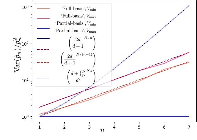
Figure 5: Maximal and minimal variance for a two-qubit system using the full-basis and partial-basis methods, as obtained by a gradient descent optimization. The results obtained for the maximally- and minimally-mixed states in Eqs. (42), (43), and (48), are presented in dashed lines for comparison.

III.4 Required number of repetitions

The method suggested makes use of random quantum states for the estimation of entanglement measures. When drawing random vectors from the probability measures indicated above, one finds for the probability of deviating from the expectation to be bounded by

$${\rm Pr}\biggl{(}|\hat{p}_{n}-\mathbb{E}(\hat{p}_{n})|\geq k\sigma(\hat{p}_{n})\biggr{)}\leq\frac{1}{k^{2}},$$ (30)

for real $k$ and $\sigma(\hat{p}_{n})^{2}:={\rm Var}(\hat{p}_{n})$. This is true by virtue of Chebychev’s inequality, a large deviation bound. We here and in the following suppress the dependence on $\rho_{A}$. For $M$ repetitions, the variance ${\text{Var}_{M}}$ of the estimator of the mean ${\mathbb{E}}(\hat{p}_{n})$ is given by

$${\text{Var}_{M}}:=\frac{\text{Var}(\hat{p}_{n})}{M}.$$ (31)

Since then

$$\varepsilon^{2}:=\frac{{\text{Var}_{M}}}{p_{n}^{2}}=\frac{\text{Var}(\hat{p}_{n})}{Mp_{n}^{2}},$$ (32)

for a given $\varepsilon>0$, the number of required repetitions scales as $M={\text{Var}(\hat{p}_{n})}/(p_{n}^{2}\varepsilon^{2})$.

The characteristics of the method lead us to expect an exponential dependence of the required number of repetitions $M$ on system size (whilst as can be seen below, a weak one). We thus define the scaling factor $\xi_{n}$ by

$$\frac{\text{Var}(\hat{p}_{n}(\rho_{A}))}{p_{n}(\rho_{A})^{2}}=:\xi_{n}^{N_{A}}.$$ (33)

We use the notation $\xi_{n}$ for the scaling factor of $\hat{R}_{n}$ as well, since the scaling factors for both properties are expected to behave similarly.

In Appendix A, we show that the variance of the estimators defined in Eqs. (23) and (25) is given by

$$\text{Var}\left(\hat{p}_{n}\right)=\mathrm{Tr}((\rho_{A}^{\otimes 2}\mathcal{E})^{n})-p_{n}(\rho_{A})^{2}$$ (34)

and

$$\text{Var}(\hat{R}_{n})=\mathrm{Tr}\left(\left((\rho_{A}^{T_{2}})^{\otimes 2}\mathcal{E}\right)^{n}\right)-R_{n}(\rho_{A})^{2},$$ (35)

where

$${\cal E}:=\mathbb{E}\left(\ket{V}\otimes\ket{V}\bra{V}\otimes\bra{V}\right).$$ (36)

Given the product structure of the probability measure, this expression is found to be $\mathcal{E}=\otimes_{\alpha\in A}\mathcal{E}^{[\alpha]}$, with

$${\cal E}^{[\alpha]}:=\mathbb{E}\left(\ket{v^{[\alpha]}}\otimes\ket{v^{[\alpha]}}\bra{v^{[\alpha]}}\otimes\bra{v}^{[\alpha]}\right).$$ (37)

In a coordinate representation, this is found to be

$$\mathcal{E}_{i,j,kl}^{[\alpha]}=\frac{d}{d+1}(\delta_{i,k}\delta_{j,l}+\delta_{i,l}\delta_{j,k})$$ (38)

for the full-basis distribution, and

$$\mathcal{E}_{i,j;k,l}^{[\alpha]}=\delta_{i,k}\delta_{j,l}+\delta_{i,l}\delta_{j,k}-\delta_{i,k}\delta_{j,l}\delta_{i,l}$$ (39)

for the partial-basis distribution. To give an even more specific example in a coordinate dependent form, for $d=2$, we have

$$\mathcal{E}^{[\alpha]}=\left(\begin{array}[]{cccc}\frac{4}{3}&0&0&0\\ 0&\frac{2}{3}&\frac{2}{3}&0\\ 0&\frac{2}{3}&\frac{2}{3}&0\\ 0&0&0&\frac{4}{3}\end{array}\right)$$ (40)

and

$$\mathcal{E}^{[\alpha]}=\left(\begin{array}[]{cccc}1&0&0&0\\ 0&1&1&0\\ 0&1&1&0\\ 0&0&0&1\end{array}\right)$$ (41)

for the full-basis and partial-basis distributions, respectively. The variance of the symmetry-resolved moments estimator is shown to be bounded from above by Eq. (34) in Appendix A.

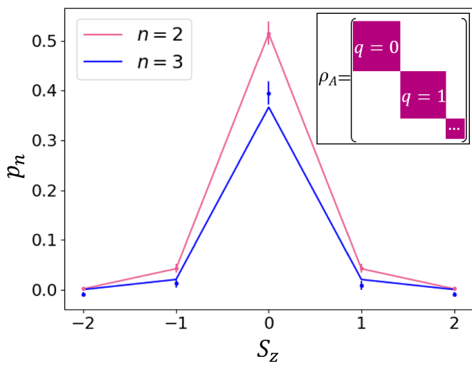
Figure 6: Symmetry-resolved RDM moments of the XX model ground state with $N_{A}=20$ and $n=2,3$. The lines are the exact values and dots are the extracted values using the partial-basis distribution, Eq. (29), with the errors estimated from the sample variance. The number of samples $M$ used is approximately $10^{2}\xi_{3}^{N_{A}},$ where $\xi_{3}=1.65$. Inset: When the RDM commutes with the charge operator $\hat{Q}_{A}$, it decomposes into blocks corresponding to different charges in subsystem $A$.

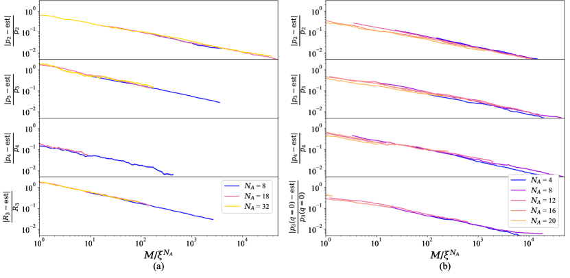
Figure 7: Relative error in the estimation of (a) the 2nd-4th RDM moments and the 3rd PT moment of the toric code ground state for a checkerboard partition ($N_{A}=w^{2}/2$), and (b) The 2nd-4th RDM moment and the 3rd symmetry-resolved RDM moment for $q=0$ of the XX model ground state, based on Eq. (23) for the RDM moments, on Eq. (25) for the PT moment and (51) for the symmetry-resolved moment. Here, we use the partial-basis distribution, Eq. (29). The normalization of $M$ by the scaling factor $\xi_{n}$ in the horizontal axis is extracted from Fig. 8 and presented in Table 1. The presented plots are averaged over 20 different permutations of the estimation results.

We first focus on discussing the full-basis distribution. As shown in Appendix A, the squared coefficient of variation in a product state $\rho=\otimes_{\alpha\in A}\ket{\psi}_{\alpha}\bra{\psi}_{\alpha}$ and in a maximally mixed case (i.e., subsystem $A$ being maximally entangled with the rest of the system), $\rho_{A}=\mathbb{I}/d^{N_{A}}$, are

$$\frac{\text{Var}(\hat{p}_{n})}{p_{n}^{2}}=\left(\frac{2d}{d+1}\right)^{nN_{A}}-1$$ (42)

and

$$\frac{\text{Var}(\hat{p}_{n})}{p_{n}^{2}}=\left(\frac{2d}{d+1}\right)^{(n-1)N_{A}}-1,$$ (43)

respectively. The same results apply for the PT moments. For example, for $d=2$,

$$\xi_{n}=\left(\frac{4}{3}\right)^{n}$$ (44)

for a product state and

$$\xi_{n}=\left(\frac{4}{3}\right)^{n-1}$$ (45)

for a maximally mixed state. Note that the scaling factors obtained below for the benchmark models, as displayed in Table 1, are in-between these two extreme cases.

As for the partial-basis distribution, as explained in detail in Appendix A, the highest variance, hence the largest additive sampling error, for both the RDM moments and PT moments arises for

$$\rho=\otimes_{\alpha\in A}\ket{\psi_{E}}\bra{\psi_{E}}_{\alpha},$$ (46)

where $\ket{\psi_{E}}$ stands for a state vector of the form

$$\ket{\psi_{E}}=\frac{1}{\sqrt{d}}\sum_{j=1}^{d}\left[e^{i\phi_{j}}\ket{j}\right],$$ (47)

with an equal magnitude of the amplitude for each state in the computational basis. In this case, the contribution of each site to the first term of the variance is

$$\xi_{n}=\left(\left(d+4\binom{d}{2}\right)/d^{2}\right)^{n},$$ (48)

and the overall variance is given by

$$\left(\left(d+4\binom{d}{2}\right)/d^{2}\right)^{nN_{A}}-1.$$ (49)

For example, for $d=2$, the scaling factor in such a case is $\xi_{n}=\left({3}/{2}\right)^{n}$. The best case is $\rho_{A}=\ket{0}\bra{0}^{\otimes N_{A}}$ (or any other basis state in the computational basis), in which the variance is 0. Both cases are completely disentangled, and the moments equal 1. Therefore, the former of these is not maximal in terms of the squared coefficient of variation, which is determined by the ratio between the standard deviation and the expected value. However, the analysis of the variance itself already serves to demonstrate that that the choice of basis for the vector $\ket{v}$ can have a significant impact on the variance and due to that on the performance of the algorithm, as discussed in Section IV.3 below. The coefficient of variation in the maximally nixed case in this method is calculated in Appendix A and equals

$$\frac{\text{Var}(\hat{p}_{n})}{p_{n}^{2}}=\left(\frac{d+\binom{d}{2}2^{n}}{d^{2}}\right)^{N_{A}}.$$ (50)

The two cases represented in Eqs. (42), (43), and (48) above, in which the variance can be calculated exactly, are not promised to be the best or worst case for the two distribution methods. For a two-qubit system we have performed a gradient descent search for the extreme cases in both distributions, where a basis optimization (as described in Section IV.3) has been included in the partial-basis method. Fig. 5 presents the results, which strongly support the hypothesis that the maximally- and minimally-mixed cases are indeed the extreme cases for the method’s performance.

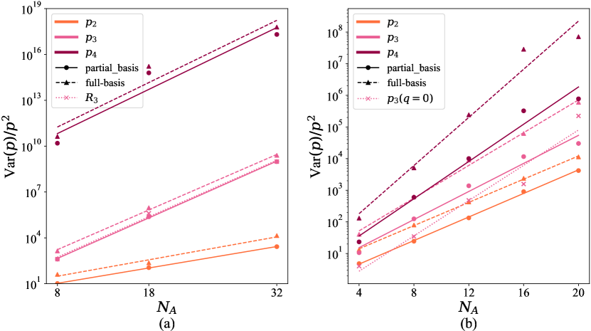
Figure 8: Numerical estimation of the variance of (a) the 2nd-4th RDM moments and the 3rd PT moment of the toric code ground state for a checkerboard partition; (b) the 2nd-4th RDM moment and the 3rd symmetry-resolved RDM moment for $q=0$ of the XX model ground state. Here, we mainly use the partial-basis distribution, Eq. (29), and add results for $p_{n}$ in the full-basis distribution, Eq. (28), which displays a very similar performance in the more strongly entangled toric code model, and a worst behaviour in the log-like entangled XX model. In the vertical axis title, $p$ stands for the estimated moment in all cases. The dependence of the variance on system size $\xi$, defined in Eq. (33), is extracted from the linear fit in the figure and shown in Table 1. Note that for the toric code ground state shown in (a), the behaviours of the 3rd RDM moment and the 3rd PT moment are expected to be identical, and are slightly different only due to the random nature of our protocol.

The best distribution choice is therefore case-dependent: For moderate or large $n$ and highly mixed cases, the full-basis distribution is advantageous. For small $n$ or weakly entangled cases, the partial-basis method with a smart basis choice (as discuss in Section IV.3) is more beneficial. Based on Eq. (50), the partial-basis seems to have a poor performance on highly entangled (mixed) states. However, states represented efficiently by TN feature an entanglement that exhibits an area law, which restrains the entanglement of relevant states to begin with. Note that even in this worst case our method is still favourable compared to the the time required for an exact diagonalization of the RDM, which scales as $O(d^{3N_{A}})$, for intermediate $n$. The variances calculated above compare favorably with the variances in the experimental sampling-based protocols(Merkel et al., 2010; Ohliger et al., 2013; van Enk and Beenakker, 2012; Tran et al., 2015; Elben et al., 2018; Ketterer et al., 2019; Brydges et al., 2019; Vermersch et al., 2019; Elben et al., 2020a; Cian et al., 2021; Knips et al., 2020; Joshi et al., 2020; Zhang et al., 2020; Huang et al., 2020; Elben et al., 2020b), as calculated in Ref.  Elben et al., 2020b: For $d=2$, the relative variances for $n=2,3$ are shown to be $\text{Var}(\hat{p}_{2})/p_{2}^{2}\geq(8/p_{2}^{2})\max\left\{2^{N_{A}}p_{2},2^{1.5N_{A}}\right\}$ and $\text{Var}(\hat{p}_{3})/p_{3}^{2}\geq\left(39/p_{3}^{2}\right)\max\left\{2^{N_{A}}p_{2}^{2},2^{1.5N_{A}}p_{2},2^{2N_{A}}\right\}$.

It would be interesting to use the analysis above as a basis for a study regarding the number of local samples required for the estimation of Rényi moments in general. Naively, the moments are defined as a function of the full RDM, which has $d^{2N_{A}}$ elements, hence should require a comparable number of samples. However, an extraction of a single degree of freedom is expected to require a smaller number of samples, as is the case in small $n$s in our method. Such analysis may point to the amount of information contained in Rényi moments of different ranks.

III.5 Symmetry-resolved RDM moments

Using the locality of the phase operator from Eq. (8), $e^{i\varphi\hat{Q}_{A}}=\otimes_{\alpha\in A}e^{i\varphi\hat{Q}_{\alpha}}$, we can extract the flux-resolved moments from the TN, and substitute them into Eq. (9) to get the symmetry-resolved moments. The estimator of the flux-resolved moment is similar to the estimator of the full moments in Eq. (23) and is obtained from

$$\hat{p}_{n}(\rho_{A},\varphi)= \bra{V^{(1)}}e^{i\varphi\hat{Q}_{A}}\rho_{A}\ket{V^{(2)}}\bra{V^{(2)}}\rho_{A}\ket{V^{(3)}}$$

$$\times\dots\bra{V^{(n)}}\rho_{A}\ket{V^{(1)}}.$$ (51)

The estimator of the charge-resolved moment is obtained from

$$\hat{p}_{n}(\rho_{A},q)= \sum_{\phi}e^{-iq\varphi}\bra{V^{(1)}}e^{i\varphi\hat{Q}_{A}}\rho_{A}\ket{V^{(2)}}\dots$$

$$\times\dots\bra{V^{(n)}}\rho_{A}\ket{V^{(1)}}.$$ (52)

A similar analysis of symmetry-resolved PT moments has been done in Ref. Cornfeld et al., 2018, and the extension to their estimation is natural. Below we estimate the symmetry-resolved RDM moments for the XX model and its conserved total $S_{z}$. For this model, the symmetry-resolved moments can be obtained exactly following Ref. Goldstein and Sela, 2018. The expected and extracted results for $q\mapsto p_{n}(\rho_{A},q)$ for $n=2,3$ are displayed in Fig. 6.

IV Testing the method against the benchmark models

IV.1 Specific tests

We have tested the model against the exactly solvable two-dimensional toric code model and one-dimensional XX model as detailed in Section II.4, employing the TensorNetwork library(Roberts et al., 2019). The precision of the estimation for both models as a function of $M$, the number of samples of the expressions in Eqs. (21), (23), (25), and (51) is shown in Fig. 7. The results are obtained using the partial-basis distribution, Eq. (29), and are optimized based on the analysis in Section IV.3 below. In order to reduce the numerical noise in the dependence of the precision in $M$, we averaged this dependence over several permutations of the $M$ repetitions. While the required number of repetitions $M$ (for a given allowed error $\varepsilon>0$) is exponential in system size (as discussed above in Section III.4), it has a relatively small base $\xi_{n}$. When considering the significant decrease in required memory space, our method can become advantageous for systems around $N_{A}=20$, for which the method described in Section II.2 can become too heavy in memory demands for a standard computer workstation.

IV.2 Variance estimation

Here we follow the analysis of the scaling factor $\xi_{n}$ in Section III.4 and estimate the scaling factors in the benchmark models, in order to get some idea regarding the variance in the general case. The scaling factors $\xi_{n}$ obtained for the toric code and XX ground states, for $n=2,3,4$ are estimated numerically. In Appendix B, we demonstrate an exact calculation of the expressions in Eqs. (34) and (35) for a narrow strip-like system in the toric code model, and show that the resulting expressions agree with the numerically estimated scaling factors.

We emphasize that the models used are not specifically suitable for the method, and are not expected to have a low scaling factors based on Eqs. (34) and (35). The estimated scaling factor $\xi_{n}$ can therefore be considered typical.

Fig. 8 presents the estimated variances of the benchmark models in the full-basis distribution and partial-basis distribution after the basis-choice optimization detailed in Section IV.3. The scaling factor can be extracted from the dependence of the variance on $N_{A}$. We see that the scaling factors are smaller than the worst case presented above. In the XX model, for which the entanglement is log-dependent in system size, we get a better performance with the basis-optimized partial-basis distribution. In the more strongly entangled (and therefore less basis-sensitive) toric code model, the difference in performance between the two methods is clearly less significant.

IV.3 Dependence on basis choice

In the partial-basis distribution, as shown above, the largest and smallest additive variance values both correspond to a completely disentangled case, and the difference between the two stems from the single-particle basis choice alone. This can be understood by the decomposition

$$\mathcal{E}^{[\alpha]}=\mathbb{I}\otimes\mathbb{I}+\frac{1}{2}\left(\sigma^{x}\otimes\sigma^{x}+\sigma^{y}\otimes\sigma^{y}\right),$$ (53)

as can be seen from Eqs. (40) and (41), that demonstrates the orientation dependence of $\mathcal{E}$ in this case (in contrast with

$$\mathcal{E}^{[\alpha]}=\mathbb{I}\otimes\mathbb{I}+\frac{1}{3}\left(\sigma^{x}\otimes\sigma^{x}+\sigma^{y}\otimes\sigma^{y}+\sigma^{z}\otimes\sigma^{z}\right)$$ (54)

in the full-basis case). For a translationally invariant system, one can expect that the optimal basis choice for each site will be the same. We can now attempt to decrease the variance by finding the basis for which $\text{Var}(\hat{p}_{1})$ is minimal, and use this basis for the estimation of higher moments. We have tested this idea against the first moment of the two benchmark models, by rotating the random vectors

$$\ket{v^{[\alpha]}}\longmapsto e^{i\phi\sigma^{x}}e^{i\theta\sigma^{y}}\ket{v^{[\alpha]}},$$ (55)

and finding the best basis, as demonstrated in Fig. 9. We plot the scaling factor for $n=1$, $\xi_{1}$, for the two benchmark models as a function of the basis choice. We then compare the best and worst choices of $\phi,\theta\in[0,2\pi)$ and extract the variance of the higher moments in the corresponding bases, as summarized in Table 1. We can see that the $p_{1}$ case acts as a good indicator for the basis choice of the moments in higher $n$s, and allows for a smart basis choice which decreases the variance.

Figure 9: $\xi_{1}$, the scaling factor of the normalized variance of the first moment with system size as defined in Eq. (33), as a function of the working basis defined by $\phi,\theta\in[0,2\pi)$ in Eq. (55) for the partial-basis distribution, Eq. (29), and for (a) the toric code ground state for a checkerboard partition and (b) the XX model ground state.

	Toric code best case	Toric code worst case	XX best case	XX worst case
$(\phi,\theta)$	$(0,0.3\pi)$	$(0.5\pi,0)$	$(0.5\pi,0.5\pi)$	$(0,0)$
$\xi_{1}$	$1.05$	$1.07$	$1.24$	$1.30$
$\xi_{2}$	$1.23$	$1.36$	$1.54$	$1.73$
$\xi_{2}$ [Full-basis]	$1.26$		$1.51$
$\xi_{3}$	$1.80$	$1.89$	$1.65$	$1.98$
$\xi_{3}$ [Full-basis]	$1.81$		$1.77$
$\xi_{4}$	$2.75$	$2.91$	$2.09$	$2.50$
$\xi_{4}$ [Full-basis]	$2.81$		$2.34$

Table 1: The extracted scaling factor defined in Eq. (33), $\xi_{n}$, for $n=2,3,4$ for the best and worst case in the toric code ground state extracted from Fig. 9 and the XX model ground state. The scaling factors obtained in the full-basis method are displayed for comparison. The worst and best case in $\xi_{1}$ are shown to predict well the dependence of $\xi_{n}$ on the basis choice.

V Conclusions and Outlook

In high-dimensional TN states, the naive computation of entanglement is highly sensitive to the size of the system (when explicitly extracting the RDM) or the bond dimension of the site tensors and boundaries (when performing the replica trick). We developed a method for estimating RDM moments in Eq. (2) and PT moments in Eq. (5) of such systems, as well as their symmetry-resolved components in Eqs. (7) and (8), without fully reconstructing the density matrix or contracting several copies of the state. The method uses randomization in order to correlate separate copies of the TN state, allowing for the estimation of properties that are defined using more than one copy of the RDM. Though we are inspired by recent experimental protocols(Tran et al., 2015; Merkel et al., 2010; van Enk and Beenakker, 2012; Ohliger et al., 2013; Elben et al., 2018; Ketterer et al., 2019; Brydges et al., 2019; Vermersch et al., 2019; Elben et al., 2020a; Cian et al., 2021; Knips et al., 2020; Joshi et al., 2020; Zhang et al., 2020; Huang et al., 2020), we developed a completely new algorithm which is suitable to classical simulations, takes advantage of their strengths such as ability to estimate the expectation value of non-Hermitian operators, and avoids their weakness in sampling the outcomes of random measurements.

We have demonstrated our method with the iPEPS representation of the toric code ground state and the MPS representation of the XX ground state, and compared the results with analytical calculations. The method can be readily used for any tensor network ansatz representing a spin or bosonic system, and provide information on the entanglement of systems that were formerly unreachable by today’s computers due to a strong exponential dependence of the memory space in the moment degree $n$. Additionally, our method is advantageous for nontrivial partitions in one or higher spatial dimensions, such as the checkerboard partition (Hsieh and Fu, 2014) or random partition (Vijay and Fu, 2015), for which the moments are hard to calculate even for one-dimensional MPS.

We compare two options for the random distribution, where each of the methods turns out to be suitable for different cases. For small $n$s, the scaling of required samples number $M$ with system size $N_{A}$ turns out to be lower than the scaling of RDM size, and can have implications regarding the information contained in these moments. It would be interesting to try and develop a sampling-based method which incorporates non-physical operations and compare its performance with ours. The analysis of such a protocol may shed more light on the power of Rényi moments.

The method should be suitable to fermionic PEPS(Barthel et al., 2009; Corboz et al., 2010), and can be generalized to additional Rényi measures, such as participation entropies, used for the detection of many-body localization(Macé et al., 2019). Exploring the possibility of derandomizing the algorithm, similarly to the recent results of Huang et al.(Huang et al., 2021) would also be interesting. In contrast to setting of shadow estimation, the very quantum state is already classically efficiently represented, and computing overlaps with suitable random vectors gives rise to an effective estimation of entanglement properties. Now that the option to use non-physical sampling has been opened, it can be expanded to various platforms, including experimental setting with a vectorized density matrix. It is the hope that this work contributes to the program of exploiting the power of random measurements in quantum physics, even in situations where the sampling scheme itself is not reflected by physical operations.

Appendix A Full derivation of the variance

Below we derive Eqs. (34), (40) and (41) of the main text, and use them to find density matrices which extremize the variance. First, we write the expression for the RDM moments estimator explicitly. In the above coordinate independent fashion, this derivation is straightforward. The $n$-th RDM moment is obtained as the expectation of

$$\hat{p}_{n}(\rho_{A})=\bra{V^{(1)}}\rho_{A}\ket{V^{(2)}}\dots\bra{V^{(n)}}\rho_{A}\ket{V^{(1)}},$$ (56)

where again, the product state vectors $\ket{V^{(1)}},\dots,\ket{V^{(n)}}$ are drawn in an i.i.d. fashion from the same probability measure. In expectation, we find

$$\mathbb{E}(\hat{p}_{n}(\rho_{A})) = \mathbb{E}(\bra{V^{(1)}}\rho_{A}\ket{V^{(2)}}\dots\bra{V^{(n)}}\rho_{A}\ket{V^{(1)}})$$

$$= \mathbb{E}(\mathrm{Tr}(\ket{V^{(1)}}\bra{V^{(1)}}\rho_{A}\ket{V^{(2)}}\dots\bra{V^{(n)}}\rho_{A}))$$

$$= \mathrm{Tr}(\rho_{A}^{n})=p_{n}(\rho_{A}).$$

Similarly, for the PT moments, one can make use of random vectors of the form

$$\ket{V^{(i,j)}}=\otimes_{\alpha\in A_{1}}\ket{[v^{[\alpha]}]^{(i)}}\otimes_{\beta\in A_{2}}\ket{[v^{[\beta]}]^{(j)}},$$ (58)

for $i,j=1,\dots,n$, so that the estimator of the negativity moment is

$$\hat{R}_{n}(\rho_{A}) = \bra{V^{(1,n)}}\rho_{A}\ket{V^{(2,n-1)}}\bra{V^{(2,n-1)}}\rho_{A}\ket{V^{(3,n-2)}}\times\dots\bra{V^{(n-1,2)}}\rho_{A}\ket{V^{(n,1)}}\bra{V^{(n,1)}}\rho_{A}\ket{V^{(1,n)}},$$

since one simply finds by performing partial transposes in all terms

$$\mathbb{E}(\hat{R}_{n}(\rho_{A})) = \mathbb{E}\mathrm{Tr}(\bra{V^{(1,n)}}\rho_{A}\ket{V^{(2,n-1)}}\bra{V^{(2,n-1)}}\rho_{A}\ket{V^{(3,n-2)}}$$

$$\times \dots\bra{V^{(n-1,2)}}\rho_{A}\ket{V^{(n,1)}}\bra{V^{(n,1)}}\rho_{A}\ket{V^{(1,n)}})$$

$$= \mathrm{Tr}\left((\rho_{A}^{T_{2}})^{n}\right),$$

so that indeed the correct moment of the partially transposed operator is recovered. The variance can then be calculated from the expectation of

$$\hat{p}_{n}(\rho_{A})^{2} = (\bra{V^{(1)}}\rho_{A}\ket{V^{(2)}})^{2}(\bra{V^{(2)}}\rho_{A}\ket{V^{(3)}})^{2}\dots(\bra{V^{(n)}}\rho_{A}\ket{V^{(1)}})^{2}$$ (60)

from which the square of $p_{n}(\rho_{A})$ is subtracted. The subtle point is now that projections appear twice rather than once. This can be reflected by making use of two tensor factors. Upon reordering the tensor entries, one immediately finds the expression

$$\hat{p}_{n}(\rho_{A})^{2} = \mathrm{Tr}\left((\bra{V^{(1)}}\otimes\bra{V^{(1)}})(\rho_{A}\otimes\rho_{A})(\ket{V^{(2)}}\otimes\ket{V^{(2)}})\dots(\bra{V^{(n)}}\otimes\bra{V^{(n)}})(\rho_{A}\otimes\rho_{A})(\ket{V^{(1)}}\otimes\ket{V^{(1)}})\right)$$ (61)

$$= \mathrm{Tr}\left(\prod_{j=1}^{n}(\ket{V^{(j)}}\otimes\ket{V^{(j)}})(\bra{V^{(j)}}\otimes\bra{V^{(j)}})(\rho_{A}\otimes\rho_{A})\right).$$ (62)

In expectation, this is $\mathbb{E}(\hat{p}_{n}(\rho_{A})^{2})=\mathrm{Tr}((\rho_{A}^{\otimes 2}\mathcal{E})^{n})$ with

$${\cal E}=\mathbb{E}\left(\ket{V}\otimes\ket{V}\bra{V}\otimes\bra{V}\right)$$ (63)

and hence $\mathcal{E}=\otimes_{\alpha\in A}\mathcal{E}^{[\alpha]}$, where

$${\cal E}^{[\alpha]}=\mathbb{E}\left(\ket{v^{[\alpha]}}\otimes\ket{v^{[\alpha]}}\bra{v^{[\alpha]}}\otimes\bra{{v}^{[\alpha]}}\right).$$ (64)

In this way, one finds the expression for the variance

$$\text{Var}(\hat{p}_{n}(\rho_{A}))=\mathrm{Tr}((\rho_{A}^{\otimes 2}\mathcal{E})^{n})-p_{n}^{2}.$$ (65)

Here it is relevant that the frames made use of do not necessarily have to constitute complex spherical 2-designs for estimating the above entanglement measures in an unbiased fashion, so that the average does not necessarily resemble that of the Haar average, and may depend on the ensemble. We now see why it is meaningful to consider the two probability measures specified above: Drawing vectors from the eigenbasis of a single Pauli matrix, i.e., randomly sampling RDM elements in this basis, would give, for example if we drew from the eigenbasis of $Z$,

$$\mathcal{E}_{i,k;j,l}^{[\alpha]}=\delta_{i,j}\delta_{k,l}+\delta_{i,k}\delta_{j,l}+\delta_{i,l}\delta_{j,k}-2\delta_{i,k}\delta_{j,l}\delta_{i,l}.$$ (66)

This matrix equals the matrix obtained above, with added positive terms, hence, can only increase the variance. The same argument can be made for any number of Pauli matrices between 2 and $d-1$. The Pauli matrices constitute a unitary 1-design Gross et al. (2007), which is the requirement for them to be a universal measure for the estimators in Eqs. (21), (23), (25), and (52). Therefore, it is unnecessary to consider additional distributions. In the maximally mixed case, $\rho_{A}=(\mathbb{I}_{d}/d)^{\otimes N_{A}}$, the normalized first term is

$$\frac{\mathrm{Tr}\left(\left[\rho_{A}^{\otimes 2}\mathcal{E}\right]^{n}\right)}{p_{n}^{2}} =\text{$\left(\frac{2d}{d+1}\right)$}^{(n-1)N_{A}}$$ (67)

for the full-basis and

$$\frac{\mathrm{Tr}\left(\left[\rho_{A}^{\otimes 2}\mathcal{E}\right]^{n}\right)}{p_{n}^{2}} =\left(\frac{d+\binom{d}{2}2^{n}}{d^{2}}\right)^{N_{A}}$$ (68)

for the partial-basis, respectively. In a product state, $\rho_{A}=\otimes_{\alpha\in A}\ket{\psi}_{\alpha}\bra{\psi}_{\alpha}$ in the full-basis distribution, one finds

$$\frac{\mathrm{Tr}\left(\left[\rho_{A}^{\otimes 2}\mathcal{E}\right]^{n}\right)}{p_{n}^{2}}=\text{$\left(\frac{2d}{d+1}\right)$}^{nN_{A}}.$$ (69)

The performance of the partial-basis distribution for a product state can be analyzed as follows: $\mathcal{E}^{[\alpha]}$ is a block diagonal matrix, with $d$ blocks of the form $B_{1}=(1)$ and $\binom{d}{2}$ blocks of the form

$$B_{2}=\left(\begin{array}[]{cc}1&1\\ 1&1\end{array}\right).$$ (70)

The largest eigenvalue of $\prod_{\alpha\in A}\mathcal{E}^{[\alpha]}$ is thus $2^{N_{A}}$, and corresponds to an eigenvector of the form $\otimes_{\alpha\in A}\ket{i,j}$, where $i$ and $j$ correspond to the spin of the site $\alpha$ in the two copies and $i,j=1,\dots,d$, for $i\neq j$. However, since $\rho_{A}^{\otimes 2}$ is constructed from two identical copies of $\rho_{A}$, vectors of the form above cannot be the only contributors to the RDM. The RDM with the largest possible variance has an equal weight to all vectors of the form above, which means it will have the form

$$\rho_{A}=\otimes_{\alpha\in A}\frac{1}{d}\left(\begin{array}[]{ccc}1&\dots&1\\ \vdots&\ddots&\vdots\\ 1&\dots&1\end{array}\right).$$ (71)

Then, the contribution of each site to the first term of the variance is

$$\xi_{n}=\left(\left(d+4\binom{d}{2}\right)/d^{2}\right)^{n}.$$ (72)

The RDM with smallest possible variance will be, for example,

$$\rho_{A}=\ket{0}\bra{0}^{\otimes N_{A}},$$ (73)

or any other product state in the computational basis. In this case, the first term of the variance sums up to 1 and $\text{Var}(\hat{p}_{n})=0$. In both cases A is disentangled from its environment, which demonstrates that the variance of the estimated value depends on the basis choice for the vectors $\ket{v}$.

The variance of the flux-resolved moment estimators of the complex valued random variable defined in Eq. (51) can similarly be computed from

$$|\hat{p}_{n}(\rho_{A},\varphi)|^{2} = \langle V_{1}|e^{i\varphi\hat{Q}_{A}}\rho_{A}|V_{2}\rangle\langle V_{2}|\rho_{A}|V_{3}\rangle\dots\langle V_{n}|\rho_{A}|V_{1}\rangle$$

$$\times \langle V_{1}|\rho_{A}|V_{n}\rangle\dots\langle V_{3}|\rho_{A}|V_{2}\rangle\langle V_{2}|\rho_{A}e^{-i\varphi\hat{Q}_{A}}\rho_{A}|V_{1}\rangle$$

$$= \mathrm{Tr}\left(\left(\rho_{A}e^{i\varphi\hat{Q}_{A}}\otimes e^{-i\varphi\hat{Q}_{A}}\rho_{A}\mathcal{E}\right)\left(\rho_{A}^{\otimes 2}\mathcal{E})^{n-1}\right)\right),$$

which is bounded from above by the variance for the non-resolved case, as the sum of the first term is composed of terms with the same absolute values, but with added phases. The estimator for the variance of the symmetry-resolved moments is therefore also bounded by

$$\text{Var}(\hat{p}_{n}(q)) = \frac{1}{N_{A}}\sum_{\varphi}\text{Var}(\hat{p}_{n}(\varphi))$$ (75)

$$\leq \frac{1}{N_{A}}\sum_{\varphi}\text{Var}(\hat{p}_{n})=\text{Var}(\hat{p}_{n}).$$

Figure 10: (a) A configuration of a strip-like subsystem of dimension $2\times 2l$, here $l=3$. (b) An example for a contributing configuration of operators to the term $\mathrm{Tr}((\rho_{A}^{\otimes 2}\mathcal{E})^{n})$ in Eqs. (34) and (35), for $n=2$ and a subsystem composed of $l=3$ stars. Depicted in pink and blue are stabilizers under which the subsystem RDM is invariant, and therefore each of them can be applied to any of the copies and contribute to the trace (Note that $\sigma^{y}=i\sigma^{z}\sigma^{x}$). In orange and purple is a pair of operators which commute with the star operator $\otimes_{i\in s}\sigma_{i}^{x}$ due to having an even number of $\sigma^{y}$ matrices. Such a pair of operators which commute with the stabilizer operator will also contribute to the trace, provided they are applied on both sides of the same copy of $\rho_{A}^{\otimes 2}$ factors. (c) An example element of the transfer matrix $T^{(2)}$. Applying the operators in orange to the $(l+1)$-th star, given that the operator configuration on the $l$-th operator is the one in pink, is allowed, and the expression will be multiplied by $2^{-4}$ due to the four $\frac{1}{2}\sigma^{y}\otimes\sigma^{y}$ applied to the $(l+1)$-th star. (d) An additional example element in the transfer matrix $T^{(2)}$. Applying the operators in orange to the $(l+1)$-th star will not contribute to the trace, since this operator configuration do not commute with the plaquette or star terms.

Appendix B Explicit variance calculation for the toric code

Here, we demonstrate how the variance can be calculated exactly in the toric code model for a subsystem shaped as a narrow strip (Fig. 10a for the partial-basis distribution, and compare it to the extracted variance. We start from Eqs. (34), (40) and (41), and the decomposition

$$\mathcal{E}^{[\alpha]}=\mathbb{I}+\frac{1}{2}\sigma^{x}\otimes\sigma^{x}+\frac{1}{2}\sigma^{y}\otimes\sigma^{y},$$ (76)

which applies for the partial-basis method in $d=2$. The full $\mathcal{E}$ matrix can be written as

$$\mathcal{E}=\sum_{\mathbf{S}}\otimes_{\alpha}S_{\alpha},$$

where $\mathbf{S}$ is an $N_{A}$-long configuration of the operators $\mathbb{I},\frac{1}{2}\sigma^{x}\otimes\sigma^{x},\frac{1}{2}\sigma^{y}\otimes\sigma^{y}$. We use the local symmetry of the toric code ground state

$$\otimes_{i\in s}\sigma_{i}^{x}\rho=\otimes_{i\in p}\sigma_{i}^{z}\rho=\rho\otimes_{i\in s}\sigma_{i}^{x}=\rho\otimes_{i\in p}\sigma_{i}^{z}=\rho,$$ (77)

in order to distinguish configurations $\mathbf{S}$ which will contribute to Eq. (34). An allowed configuration $\mathbf{S}$ will contain any number of star ($\otimes_{i\in s}\sigma_{i}^{x}$) or plaquette ($\otimes_{i\in p}\sigma_{i}^{z}$) operators, also called the stabilizers. Pairs of some operator which commutes with the stabilizers and act on two sides of the same copy of $\rho^{\otimes 2}$ are also allowed, as well as combinations of operators which can be transformed into such pairs by a multiplication of the operators by stabilizers. This is illustrated in Fig. 10b.

Figure 11: The estimated variances of a strip-like system in the toric code model.

	Exact variance	Estimated variance
$n=1$	$O\left(1.016^{N_{A}}\right)$	$O\left(1.016^{N_{A}}\right)$
$n=2$	$O\left(1.225^{N_{A}}\right)$	$O\left(1.220^{N_{A}}\right)$
$n=3$	$O(1.549^{N_{A}})$	$O\left(1.564^{N_{A}}\right)$

Table 2: Exact dependence of the variance on system size for the toric code model as calculated in by the transfer matrix method compared to the variance estimated from sampling of the expressions in Eqs. (34) and (35).

We calculate the variance for a narrow system of dimension $2\times 2l$, as depicted in Fig. 10a. Such a system is composed of a chain of $l$ contiguous stars. For a moment of rank $n$, we think of $n$ copies of the subsystem, and write a $3^{4n}$-dimensional vector of combinations of operators $\left[\mathbb{I},\sigma^{x}\otimes\sigma^{x},\sigma^{y}\otimes\sigma^{y}\right]$ on a single star in all $n$ copies. We now write a transfer matrix $T^{(n)}$ which takes the operator combinations on the $l$-th star to the contributing combinations on the $(l+1)$-th star: $T_{\mathbf{i},\mathbf{j}}^{(n)}$ equals the contribution of an operator combination with operators $\mathbf{j}$ on the $(l+1)$-th star to the variance in Eq. (34), given that the combination on the $l$-th star is $\mathbf{i}$, where the symmetries in Eq. (77) are considered, as well as the $\frac{1}{2}$ factors in Eq. (76). For clarity, we give a specific example in Fig. 10c-d. With these definitions, the first term in the left side of Eq. (34) for a subsystem of $2\times 2l$ sites is $\bra{c_{0}}(T^{(n)})^{l-1}\ket{c_{0}}$, where $\ket{c_{0}}$ is the vector of allowed contributions for the edges of the subsystem as can be deduced from the ground states of the toric code model in Eq. (14). The dependence of this term in the system size is thus $O\left(\lambda_{\max}^{4l}\right)$, where

$$\lambda_{\rm max}:=\|T^{(n)}\|$$ (78)

is the largest eigenvalue of the Hermitian $T^{(n)}$. One may, in fact, work with equivalent but much smaller transfer matrices, by considering only the two left sites of a star rather than the whole star. This allows decreasing the transfer matrix to dimension $3^{2n}\times 3^{2n}$. For $n\leq 3$ the matrix $T^{(n)}$ can be extracted and diagonalized exactly. We have performed an estimation of the variance for such strip-like systems, similarly to the one done in Fig. 8 in the main text. The estimated variances are displayed in Fig. 11. We have compared the results obtained exactly using the transfer matrix to the numerical variances and got a good agreement, demonstrating the accuracy of our PEPS calculations, as can be seen in the Table 2.

References

- Bennett et al. (1993) C. H. Bennett, G. Brassard, C. Crépeau, R. Jozsa, A. Peres, and W. K. Wootters, “Teleporting an unknown quantum state via dual classical and Einstein-Podolsky-Rosen channels,” Phys. Rev. Lett. 70, 1895–1899 (1993).
- Horodecki et al. (2009) R. Horodecki, P. Horodecki, M. Horodecki, and K. Horodecki, “Quantum entanglement,” Rev. Mod. Phys. 81, 865–942 (2009).
- Eisert et al. (2010) J. Eisert, M. Cramer, and M. B. Plenio, “Area laws for the entanglement entropy,” Rev. Mod. Phys. 82, 277–306 (2010).
- Verstraete et al. (2008) F. Verstraete, V. Murg, and J. I. Cirac, “Matrix product states, projected entangled pair states, and variational renormalization group methods for quantum spin systems,” Adv. Phys. 57, 143–224 (2008).
- Orús (2014) R. Orús, “A practical introduction to tensor networks: Matrix product states and projected entangled pair states,” Ann. Phys. 349, 117–158 (2014).
- Osborne and Nielsen (2002) T. J. Osborne and M. A. Nielsen, “Entanglement in a simple quantum phase transition,” Phys. Rev. A 66, 032110 (2002).
- Amico et al. (2008) L. Amico, R. Fazio, A. Osterloh, and V. Vedral, “Entanglement in many-body systems,” Rev. Mod. Phys. 80, 517–576 (2008).
- Eisert (2013) J. Eisert, “Entanglement and tensor network states,” Modeling and Simulation 3, 520 (2013).
- Xie et al. (2019) B. Z. Xie, C. D.-L. Zhou, and X.-G. Wen, Quantum information meets quantum matter: From quantum entanglement to topological phases of many-body systems (Springer, Berlin, 2019).
- Merkel et al. (2010) S. T. Merkel, C. A. Riofrío, S. T. Flammia, and I. H. Deutsch, “Random unitary maps for quantum state reconstruction,” Phys. Rev. A 81, 032126 (2010).
- Ohliger et al. (2013) M. Ohliger, V. Nesme, and J. Eisert, “Efficient and feasible state tomography of quantum many-body systems,” New J. Phys. 15, 015024 (2013).
- van Enk and Beenakker (2012) S. J. van Enk and C. W. J. Beenakker, “Measuring on single copies of using random measurements,” Phys. Rev. Lett. 108, 110503 (2012).
- Tran et al. (2015) M. C. Tran, B. Dakić, F. Arnault, W. Laskowski, and T. Paterek, “Quantum entanglement from random measurements,” Phys. Rev. A 92, 050301 (2015).
- Elben et al. (2018) A. Elben, B. Vermersch, M. Dalmonte, J. I. Cirac, and P. Zoller, “Rényi entropies from random quenches in atomic hubbard and spin models,” Phys. Rev. Lett. 120, 050406 (2018).
- Ketterer et al. (2019) A. Ketterer, N. Wyderka, and O. Gühne, “Characterizing multipartite entanglement with moments of random correlations,” Phys. Rev. Lett. 122, 120505 (2019).
- Brydges et al. (2019) T. Brydges, A. Elben, P. Jurcevic, B. Vermersch, C. Maier, B. P. Lanyon, P. Zoller, R. Blatt, and C. F. Roos, “Probing Rényi entanglement entropy via randomized measurements,” Science 364, 260–263 (2019).
- Vermersch et al. (2019) B. Vermersch, A. Elben, L. M. Sieberer, N. Y. Yao, and P. Zoller, “Probing scrambling using statistical correlations between randomized measurements,” Phys. Rev. X 9, 021061 (2019).
- Elben et al. (2020a) A. Elben, B. Vermersch, R. van Bijnen, C. Kokail, T. Brydges, C. Maier, M. K. Joshi, R. Blatt, C. F. Roos, and P. Zoller, “Cross-platform verification of intermediate scale quantum devices,” Phys. Rev. Lett. 124, 010504 (2020a).
- Cian et al. (2021) Z.-P. Cian, H. Dehghani, A. Elben, B. Vermersch, G. Zhu, M. Barkeshli, P. Zoller, and M. Hafezi, “Many-body Chern number from statistical correlations of randomized measurements,” Phys. Rev. Lett. 126, 050501 (2021).
- Knips et al. (2020) L. Knips, J. Dziewior, W. Kłobus, W. Laskowski, T. Paterek, P. J. Shadbolt, H. Weinfurter, and J. D. A. Meinecke, “Multipartite entanglement analysis from random correlations,” npj Quant. Inf. 6, 51 (2020).
- Joshi et al. (2020) M. K. Joshi, A. Elben, B. Vermersch, T. Brydges, C. Maier, P. Zoller, R. Blatt, and C. F. Roos, “Quantum information scrambling in a trapped-ion quantum simulator with tunable range interactions,” Phys. Rev. Lett. 124, 240505 (2020).
- Zhang et al. (2020) W.-H. Zhang, C. Zhang, Z. Chen, X.-X. Peng, X.-Y. Xu, P. Yin, S. Yu, X.-J. Ye, Y.-J. Han, J.-S. Xu, G. Chen, C.-F. Li, and G.-C. Guo, “Experimental optimal verification of entangled states using local measurements,” Phys. Rev. Lett. 125, 030506 (2020).
- Huang et al. (2020) H.-Y. Huang, R. Kueng, and J. Preskill, “Predicting many properties of a quantum system from very few measurements,” Nature Phys. 16, 1050–1057 (2020).
- Elben et al. (2020b) A. Elben, R. Kueng, H.-Y. Huang, R. van Bijnen, C. Kokail, M. Dalmonte, P. Calabrese, B. Kraus, J. Preskill, P. Zoller, and B. Vermersch, “Mixed-state entanglement from local randomized measurements,” Phys. Rev. Lett. 125, 200501 (2020b).
- Helsen et al. (2021) J. Helsen, M. Ioannou, I. Roth, J. Kitzinger, E. Onorati, A. H. Werner, and J. Eisert, “Estimating gate-set properties from random sequences,” arXiv:2110.13178 (2021).
- Neven et al. (2021) A. Neven, J. Carrasco, V. Vitale, C. Kokail, A. Elben, M. Dalmonte, P. Calabrese, P. Zoller, B. Vermersch, R. Kueng, and B. Kraus, “Symmetry-resolved entanglement detection using partial transpose moments,” npj Quant. Inf. 7, 152 (2021).
- Gross et al. (2007) D. Gross, K. Audenaert, and J. Eisert, “Evenly distributed unitaries: On the structure of unitary designs,” J. Math. Phys. 48, 052104 (2007).
- Renes (2004) J. Renes, “Frames, designs, and spherical codes in quantum information theory,” (2004), PhD thesis, California Institute of Technology.
- Wilde (2016) M. M. Wilde, From classical to quantum Shannon theory (Cambridge University Press, 2016).
- Bennett et al. (1996) C. H. Bennett, D. P. DiVincenzo, J. A. Smolin, and W. K. Wootters, “Mixed-state entanglement and quantum error correction,” Phys. Rev. A 54, 3824–3851 (1996).
- Hill and Wootters (1997) S. Hill and W. K. Wootters, “Entanglement of a pair of quantum bits,” Phys. Rev. Lett. 78, 5022–5025 (1997).
- Życzkowski et al. (1998) K. Życzkowski, P. Horodecki, A. Sanpera, and M. Lewenstein, “Volume of the set of separable states,” Phys. Rev. A 58, 883–892 (1998).
- Rungta et al. (2001) P. Rungta, V. Bužek, Carlton M. Caves, M. Hillery, and G. J. Milburn, “Universal state inversion and concurrence in arbitrary dimensions,” Phys. Rev. A 64, 042315 (2001).
- Horodecki (2001) M. Horodecki, Entanglement measures (Rinton Press, 2001).
- Vidal and Werner (2002) G. Vidal and R. F. Werner, “Computable measure of entanglement,” Phys. Rev. A 65, 032314 (2002).
- Kim (2010) J. S. Kim, “Tsallis entropy and entanglement constraints in multiqubit systems,” Phys. Rev. A 81, 062328 (2010).
- Yang et al. (2021) X. Yang, M.-X. Luo, Y.-H. Yang, and S.-M. Fei, “Parametrized entanglement monotone,” Phys. Rev. A 103, 052423 (2021).
- Von Neumann (1932) J. Von Neumann, Mathematical foundations of quantum mechanics (Berlin, Springer, 1932).
- Daley et al. (2012) A. J. Daley, H. Pichler, J. Schachenmayer, and P. Zoller, “Measuring entanglement growth in quench dynamics of bosons in an optical lattice,” Phys. Rev. Lett. 109, 020505 (2012).
- Islam et al. (2015) R. Islam, R. Ma, P. M. Preiss, M. Eric Tai, A. Lukin, M. Rispoli, and M. Greiner, “Measuring entanglement entropy in a quantum many-body system,” Nature 528, 77–83 (2015).
- Pichler et al. (2016) H. Pichler, G. Zhu, A. Seif, P. Zoller, and M. Hafezi, “Measurement protocol for the entanglement spectrum of cold atoms,” Phys. Rev. X 6, 041033 (2016).
- Cornfeld et al. (2019a) E. Cornfeld, E. Sela, and M. Goldstein, “Measuring fermionic entanglement: Entropy, negativity, and spin structure,” Phys. Rev. A 99, 062309 (2019a).
- Eisert and Plenio (1999) J. Eisert and M. B. Plenio, “A comparison of entanglement measures,” J. Mod. Opt. 46, 145 (1999).
- Eisert (2001) J. Eisert, “Entanglement in quantum information theory,” (2001), PhD thesis, University of Potsdam.
- Peres (1996) A. Peres, “Separability criterion for density matrices,” Phys. Rev. Lett. 77, 1413–1415 (1996).
- Hor (1996) “Information-theoretic aspects of inseparability of mixed states,” Phys. Rev. A 54, 1838–1843 (1996).
- Gray et al. (2018) J. Gray, L. Banchi, A. Bayat, and S. Bose, “Machine-learning-assisted many-body entanglement measurement,” Phys. Rev. Lett. 121, 150503 (2018).
- Laflorencie and Rachel (2014) N. Laflorencie and S. Rachel, “Spin-resolved entanglement spectroscopy of critical spin chains and Luttinger liquids,” J. Stat. Mech. 2014, P11013 (2014).
- Goldstein and Sela (2018) M. Goldstein and E. Sela, “Symmetry-resolved entanglement in many-body systems,” Phys. Rev. Lett. 120, 200602 (2018).
- Xavier et al. (2018) J. C. Xavier, F. C. Alcaraz, and G. Sierra, “Equipartition of the entanglement entropy,” Phys. Rev. B 98, 041106 (2018).
- Barghathi et al. (2018) H. Barghathi, C. M. Herdman, and A. Del Maestro, “Rényi generalization of the accessible entanglement entropy,” Phys. Rev. Lett. 121, 150501 (2018).
- Cornfeld et al. (2018) E. Cornfeld, M. Goldstein, and E. Sela, “Imbalance entanglement: Symmetry decomposition of negativity,” Phys. Rev. A 98, 032302 (2018).
- Cornfeld et al. (2019b) E. Cornfeld, L. A. Landau, K. Shtengel, and E. Sela, “Entanglement spectroscopy of non-Abelian anyons: Reading off quantum dimensions of individual anyons,” Phys. Rev. B 99, 115429 (2019b).
- Feldman and Goldstein (2019) N. Feldman and M. Goldstein, “Dynamics of charge-resolved entanglement after a local quench,” Phys. Rev. B 100, 235146 (2019).
- Fraenkel and Goldstein (2020) S. Fraenkel and M. Goldstein, “Symmetry resolved entanglement: Exact results in 1D and beyond,” J. Stat. Mech. 2020, 033106 (2020).
- Murciano et al. (2020) S. Murciano, G. Di Giulio, and P. Calabrese, “Symmetry resolved entanglement in gapped integrable systems: A corner transfer matrix approach,” SciPost Phys. 8, 46 (2020).
- Capizzi et al. (2020) L. Capizzi, P. Ruggiero, and P. Calabrese, “Symmetry resolved entanglement entropy of excited states in a CFT,” J. Stat. Mech. 2020, 073101 (2020).
- Parez et al. (2021) G. Parez, R. Bonsignori, and P. Calabrese, “Quasiparticle dynamics of symmetry-resolved entanglement after a quench: Examples of conformal field theories and free fermions,” Phys. Rev. B 103, L041104 (2021).
- Tan and Ryu (2020) M. T. Tan and S. Ryu, “Particle number fluctuations, Rényi entropy, and symmetry-resolved entanglement entropy in a two-dimensional Fermi gas from multidimensional bosonization,” Phys. Rev. B 101, 235169 (2020).
- Fuji and Ashida (2020) Y. Fuji and Y. Ashida, “Measurement-induced quantum criticality under continuous monitoring,” Phys. Rev. B 102, 054302 (2020).
- Azses et al. (2020) D. Azses, R. Haenel, Y. Naveh, R. Raussendorf, E. Sela, and E. G. Dalla Torre, “Identification of symmetry-protected topological states on noisy quantum computers,” Phys. Rev. Lett. 125, 120502 (2020).
- Azses and Sela (2020) D. Azses and E. Sela, “Symmetry-resolved entanglement in symmetry-protected topological phases,” Phys. Rev. B 102, 235157 (2020).
- Estienne et al. (2021) B. Estienne, Y. Ikhlef, and A. Morin-Duchesne, “Finite-size corrections in critical symmetry-resolved entanglement,” SciPost Phys. 10, 54 (2021).
- Zhao et al. (2021) S. Zhao, C. Northe, and R. Meyer, “Symmetry-resolved entanglement in AdS3/CFT2 coupled to Chern-Simons theory,” JHEP 2021, 30 (2021).
- Vitale et al. (2021) V. Vitale, A. Elben, R. Kueng, A. Neven, J. Carrasco, B. Kraus, P. Zoller, P. Calabrese, B. Vermersch, and M. Dalmonte, “Symmetry-resolved dynamical purification in synthetic quantum matter,” arXiv:2101.07814 (2021).
- Fraenkel and Goldstein (2021) S. Fraenkel and M. Goldstein, “Entanglement measures in a nonequilibrium steady state: Exact results in one dimension,” SciPost Phys. 11, 85 (2021).
- Lukin et al. (2019) A. Lukin, M. Rispoli, R. Schittko, M. E. Tai, A. M. Kaufman, S. Choi, V. Khemani, J. Léonard, and M. Greiner, “Probing entanglement in a many-body-localized system,” Science 364, 256–260 (2019).
- Jordan et al. (2008a) J. Jordan, R. Orús, G. Vidal, F. Verstraete, and J. I. Cirac, “Classical simulation of infinite-size quantum lattice systems in two spatial dimensions,” Phys. Rev. Lett. 101, 250602 (2008a).
- Schuch et al. (2008) N. Schuch, M. M. Wolf, F. Verstraete, and J. I. Cirac, “Entropy scaling and simulability by matrix product states,” Phys. Rev. Lett. 100, 030504 (2008).
- White (1992) S. R. White, “Density matrix formulation for quantum renormalization groups,” Phys. Rev. Lett. 69, 2863–2866 (1992).
- Vidal (2004) G. Vidal, “Efficient simulation of one-dimensional quantum many-body systems,” Phys. Rev. Lett. 93, 040502 (2004).
- Verstraete et al. (2004) F. Verstraete, J. J. García-Ripoll, and J. I. Cirac, “Matrix product density operators: Simulation of finite-temperature and dissipative systems,” Phys. Rev. Lett. 93, 207204 (2004).
- Zwolak and Vidal (2004) M. Zwolak and G. Vidal, “Mixed-state dynamics in one-dimensional quantum lattice systems: A time-dependent superoperator renormalization algorithm,” Phys. Rev. Lett. 93, 207205 (2004).
- Weimer et al. (2021) H. Weimer, A. Kshetrimayum, and R. Orús, “Simulation methods for open quantum many-body systems,” Rev. Mod. Phys. 93, 015008 (2021).
- Vidal (2003) G. Vidal, “Efficient classical simulation of slightly entangled quantum computations,” Phys. Rev. Lett. 91, 147902 (2003).
- White and Feiguin (2004) S. R. White and A. E. Feiguin, “Real-time evolution using the density matrix renormalization group,” Phys. Rev. Lett. 93, 076401 (2004).
- Orús and Vidal (2008) R. Orús and G. Vidal, “Infinite time-evolving block decimation algorithm beyond unitary evolution,” Phys. Rev. B 78, 155117 (2008).
- Paeckel et al. (2019) S. Paeckel, T. Köhler, A. Swoboda, S. R. Manmana, U. Schollwöck, and C. Hubig, “Time-evolution methods for matrix-product states,” Ann. Phys. 411, 167998 (2019).
- Schollwöck (2011) U. Schollwöck, “The density-matrix renormalization group in the age of matrix product states,” Ann. Phys. 326, 96 – 192 (2011).
- Pollmann et al. (2010) F. Pollmann, A. M. Turner, E. Berg, and M. Oshikawa, “Entanglement spectrum of a topological phase in one dimension,” Phys. Rev. B 81, 064439 (2010).
- Schuch et al. (2011) N. Schuch, D. Perez-Garcia, and I. Cirac, “Classifying quantum phases using matrix product states and projected entangled pair states,” Phys. Rev. B 84, 165139 (2011).
- Pollmann et al. (2012) F. Pollmann, E. Berg, A. M. Turner, and M. Oshikawa, “Symmetry protection of topological phases in one-dimensional quantum spin systems,” Phys. Rev. B 85, 075125 (2012).
- Kshetrimayum et al. (2015) A. Kshetrimayum, Hong-Hao Tu, and R. Orús, “All spin-1 topological phases in a single spin-2 chain,” Phys. Rev. B 91, 205118 (2015).
- Cirac et al. (2020) J. I. Cirac, D. Perez-Garcia, N. Schuch, and F. Verstraete, “Matrix product states and projected entangled pair states: Concepts, symmetries, and theorems,” (2020), arXiv:2011.12127 .
- Ruggiero et al. (2016) P. Ruggiero, V. Alba, and P. Calabrese, “Entanglement negativity in random spin chains,” Phys. Rev. B 94, 035152 (2016).
- Verstraete and Cirac (2004) F. Verstraete and J. I. Cirac, “Renormalization algorithms for quantum-many body systems in two and higher dimensions,” e-print cond-mat/0407066 (2004).
- Jordan et al. (2008b) J. Jordan, R. Orús, G. Vidal, F. Verstraete, and J. I. Cirac, “Classical simulation of infinite-size quantum lattice systems in two spatial dimensions,” Phys. Rev. Lett. 101, 250602 (2008b).
- Corboz (2016) P. Corboz, “Improved energy extrapolation with infinite projected entangled-pair states applied to the two-dimensional Hubbard model,” Phys. Rev. B 93, 045116 (2016).
- Liao et al. (2017) H. J. Liao, Z. Y. Xie, J. Chen, Z. Y. Liu, H. D. Xie, R. Z. Huang, B. Normand, and T. Xiang, “Gapless spin-liquid ground state in the Kagome antiferromagnet,” Phys. Rev. Lett. 118, 137202 (2017).
- Picot et al. (2016) T. Picot, M. Ziegler, R. Orús, and D. Poilblanc, “Spin- Kagome quantum antiferromagnets in a field with tensor networks,” Phys. Rev. B 93, 060407 (2016).
- Kshetrimayum et al. (2016) A. Kshetrimayum, T. Picot, R. Orús, and D. Poilblanc, “Spin- Kagome XXZ model in a field: Competition between lattice nematic and solid orders,” Phys. Rev. B 94, 235146 (2016).
- Kshetrimayum et al. (2020a) A. Kshetrimayum, C. Balz, B. Lake, and J. Eisert, “Tensor network investigation of the double layer Kagome compound ,” Ann. Phys. 421, 168292 (2020a).
- Boos et al. (2019) C. Boos, S. P. G. Crone, I. A. Niesen, P. Corboz, K. P. Schmidt, and F. Mila, “Competition between intermediate plaquette phases in under pressure,” Phys. Rev. B 100, 140413 (2019).
- Czarnik et al. (2012) P. Czarnik, L. Cincio, and J. Dziarmaga, “Projected entangled pair states at finite temperature: Imaginary time evolution with ancillas,” Phys. Rev. B 86, 245101 (2012).
- Kshetrimayum et al. (2019) A. Kshetrimayum, M. Rizzi, J. Eisert, and R. Orús, “Tensor network annealing algorithm for two-dimensional thermal states,” Phys. Rev. Lett. 122, 070502 (2019).
- Mondal et al. (2020) S. Mondal, A. Kshetrimayum, and T. Mishra, “Two-body repulsive bound pairs in a multibody interacting Bose-Hubbard model,” Phys. Rev. A 102, 023312 (2020).
- Kshetrimayum et al. (2017) A. Kshetrimayum, H. Weimer, and R. Orús, “A simple tensor network algorithm for two-dimensional steady states,” Nature Comm. 8, 1291 (2017).
- Czarnik et al. (2019) P. Czarnik, J. Dziarmaga, and P. Corboz, “Time evolution of an infinite projected entangled pair state: An efficient algorithm,” Phys. Rev. B 99, 035115 (2019).
- Hubig and Cirac (2019) C. Hubig and J. I. Cirac, “Time-dependent study of disordered models with infinite projected entangled pair states,” SciPost Phys. 6, 31 (2019).
- Kshetrimayum et al. (2020b) A. Kshetrimayum, M. Goihl, and J. Eisert, “Time evolution of many-body localized systems in two spatial dimensions,” Phys. Rev. B 102, 235132 (2020b).
- Kshetrimayum et al. (2021) A. Kshetrimayum, M. Goihl, D. M. Kennes, and J. Eisert, “Quantum time crystals with programmable disorder in higher dimensions,” Phys. Rev. B 103, 224205 (2021).
- Dziarmaga (2021) J. Dziarmaga, “Simulation of many body localization and time crystals in two dimensions with the neighborhood tensor update,” , arXiv:2112.11457 (2021).
- Barthel et al. (2009) T. Barthel, C. Pineda, and J. Eisert, “Contraction of fermionic operator circuits and the simulation of strongly correlated fermions,” Phys. Rev. A 80, 042333 (2009).
- Corboz et al. (2010) P. Corboz, R. Orús, B. Bauer, and G. Vidal, “Simulation of strongly correlated fermions in two spatial dimensions with fermionic projected entangled-pair states,” Phys. Rev. B 81, 165104 (2010).
- Schuch et al. (2007) N. Schuch, M. M. Wolf, F. Verstraete, and J. I. Cirac, “Computational complexity of projected entangled pair states,” Phys. Rev. Lett. 98, 140506 (2007).
- Haferkamp et al. (2020a) J. Haferkamp, D. Hangleiter, J. Eisert, and M. Gluza, “Contracting projected entangled pair states is average-case hard,” Phys. Rev. Research 2, 013010 (2020a).
- Nishino and Okunishi (1996) T. Nishino and K. Okunishi, “Corner transfer matrix renormalization group method,” J. Phys. Soc. Jap. 65, 891–894 (1996).
- Orús and Vidal (2009) R. Orús and G. Vidal, “Simulation of two-dimensional quantum systems on an infinite lattice revisited: Corner transfer matrix for tensor contraction,” Phys. Rev. B 80, 094403 (2009).
- Xie et al. (2012) Z. Y. Xie, J. Chen, M. P. Qin, J. W. Zhu, L. P. Yang, and T. Xiang, “Coarse-graining renormalization by higher-order singular value decomposition,” Phys. Rev. B 86, 045139 (2012).
- Schwarz et al. (2017) M. Schwarz, O. Buerschaper, and J. Eisert, “Approximating local observables on projected entangled pair states,” Phys. Rev. A 95, 060102 (2017).
- Orús et al. (2014) R. Orús, T.-C. Wei, O. Buerschaper, and A. García-Saez, “Topological transitions from multipartite entanglement with tensor networks: A procedure for sharper and faster characterization,” Phys. Rev. Lett. 113, 257202 (2014).
- Kitaev (2003) A. Yu. Kitaev, “Fault-tolerant quantum computation by anyons,” Ann. Phys. 303, 2 – 30 (2003).
- Verstraete et al. (2006) F. Verstraete, M. M. Wolf, D. Perez-Garcia, and J. I. Cirac, “Criticality, the area law, and the computational power of projected entangled pair states,” Phys. Rev. Lett. 96, 220601 (2006).
- Hamma et al. (2005) A. Hamma, R. Ionicioiu, and P. Zanardi, “Bipartite entanglement and entropic boundary law in lattice spin systems,” Phys. Rev. A 71, 022315 (2005).
- Hsieh and Fu (2014) T. H. Hsieh and L. Fu, “Bulk entanglement spectrum reveals quantum criticality within a topological state,” Phys. Rev. Lett. 113, 106801 (2014).
- Vijay and Fu (2015) S. Vijay and L. Fu, “Entanglement spectrum of a random partition: Connection with the localization transition,” Phys. Rev. B 91, 220101 (2015).
- Kitaev and Preskill (2006) A. Kitaev and J. Preskill, “Topological entanglement entropy,” Phys. Rev. Lett. 96, 110404 (2006).
- Levin and Wen (2006) M. Levin and X.-G. Wen, “Detecting topological order in a ground state wave function,” Phys. Rev. Lett. 96, 110405 (2006).
- Jordan and Wigner (1928) P. Jordan and E. Wigner, “Über das Paulische Äquivalenzverbot,” Z. Phys. 47, 631–651 (1928).
- Peschel (2003) I. Peschel, “Calculation of reduced density matrices from correlation functions,” J. Phys. A 36, L205–L208 (2003).
- Calabrese and Cardy (2009) P. Calabrese and J. Cardy, “Entanglement entropy and conformal field theory,” J. Phys. A 42, 504005 (2009).
- Jin and Korepin (2004) B.-Q. Jin and V. E. Korepin, “Quantum spin chain, toeplitz determinants and the fisher—hartwig conjecture,” J. Stat. Phys. 116, 79–95 (2004).
- Ferris and Vidal (2012) A. J. Ferris and G. Vidal, “Perfect sampling with unitary tensor networks,” Phys. Rev. B 85, 165146 (2012).
- Bermejo-Vega et al. (2018) J. Bermejo-Vega, D. Hangleiter, M. Schwarz, R. Raussendorf, and J. Eisert, “Architectures for quantum simulation showing a quantum speedup,” Phys. Rev. X 8, 021010 (2018).
- Haferkamp et al. (2020b) J. Haferkamp, D. Hangleiter, J. Eisert, and M. Gluza, “Contracting projected entangled pair states is average-case hard,” Phys. Rev. Res. 2, 013010 (2020b).
- Roberts et al. (2019) C. Roberts, A. Milsted, M. Ganahl, A. Zalcman, B. Fontaine, Y. Zou, J. Hidary, G. Vidal, and S. Leichenauer, “TensorNetwork: A library for physics and machine learning,” (2019), arXiv:1905.01330 .
- Macé et al. (2019) N. Macé, F. Alet, and N. Laflorencie, “Multifractal scalings across the many-body localization transition,” Phys. Rev. Lett. 123, 180601 (2019).
- Huang et al. (2021) H.-Y. Huang, R. Kueng, and J. Preskill, “Efficient estimation of pauli observables by derandomization,” Phys. Rev. Lett. 127, 030503 (2021).