The star formation burstiness and ionizing efficiency of low-mass galaxies

Abstract

We investigate the burstiness of star formation and the ionizing efficiency of a large sample of galaxies at $0.7<z<1.5$ using HST grism spectroscopy and deep ultraviolet (UV) imaging in the GOODS-N and GOODS-S fields. The star formation history (SFH) in these strong emission line low-mass galaxies indicates an elevated star formation rate (SFR) based on the H$\alpha$ emission line at a given stellar mass when compared to the standard main sequence. Moreover, when comparing the H$\alpha$ and UV SFR indicators, we find that an excess in SFR_Hα compared to SFR_UV is preferentially observed in lower-mass galaxies below $10^{9}$ M_⊙, which are also the highest-EW galaxies. These findings suggest that the burstiness parameters of these strong emission line galaxies may differ from those inferred from hydrodynamical simulations and previous observations. For instance, a larger burstiness duty cycle would explain the observed SFR_Hα excess. We also estimate the ionizing photon production efficiency $\xi_{\mathrm{ion}}$, finding a median value of Log($\xi_{\mathrm{ion}}$/erg^-1 Hz)$=24.80\pm 0.26$ when adopting a Galactic dust correction for H$\alpha$ and an SMC one for the stellar component. We observe an increase of $\xi_{\mathrm{ion}}$ with redshift, further confirming similar results at higher redshifts. We also find that $\xi_{\mathrm{ion}}$ is strongly correlated with $EW_{\mathrm{H}\alpha}$, which provides an approach for deriving $\xi_{\mathrm{ion}}$ in early galaxies. We observe that lower-mass, lower-luminosity galaxies have a higher $\xi_{\mathrm{ion}}$. Overall, these results provide further support for faint galaxies playing a major role in the reionization of the Universe.

1 Introduction

There is a growing interest in the study of low-mass galaxies at all epochs, both on the theoretical and observational fronts. Until recently, most of the efforts were dedicated to characterizing massive galaxy populations out to the highest redshifts, and little was known about high$-z$ star-forming galaxies with stellar masses below $10^{10}$ M_⊙. Near-infrared spectroscopic surveys from space, such as 3D-HST (Brammer et al., 2012) and WISPS (Atek et al., 2010), and subsequent follow-ups with ground-based multi-object spectrographs (e.g., Wisnioski et al., 2015; Kriek et al., 2015), have given access to the main rest-frame optical emission lines, which enable us to derive the physical properties of the ISM in high-redshift galaxies. In particular, various studies have recently focused on investigating the star formation histories of low-mass galaxies and how they compare to their massive counterparts (e.g., Guo et al., 2016; Sparre et al., 2017; Flores Velázquez et al., 2020).

In the classic picture of galaxy evolution in which the SFR varies smoothly with time, star-forming galaxies follow a well known relation between the SFR and the stellar mass M_⋆ (e.g., Brinchmann et al., 2004; Elbaz et al., 2007; Wuyts et al., 2011b; Whitaker et al., 2014). It is believed that such a relation is shaped by the complex interplay between several physical mechanisms that operate over long timescales (Giga years). For instance, the current SFR depends on the gas accretion and the merger history of the galaxy and star-formation suppression by the AGN feedback. While this relation is expected to hold for relatively massive galaxies (> $10^{10}$ M_⊙), it is unlikely that star formation quenching from AGN remains very efficient in low-mass galaxies. Supernova explosions become the most significant source of feedback processes. At a given redshift, low-mass galaxies appear to have a higher specific star formation rate (sSFR, which is the SFR per unit of stellar mass) than "normal" galaxies, and can double their total stellar mass on a very short timescale of 100 Myr (Rodighiero et al., 2011; Atek et al., 2014; Boogaard et al., 2018). Star formation is expected to occur mostly through a stochastic process in these galaxies as a result of two competing processes: gas accretion feeding intense bursts of star formation and feedback from supernova explosions. Such variations are expected to occur on short time scales ($\sim 10$ Myr) and imply that galaxy observables might not be representative of the averaged properties of galaxies (Domínguez et al., 2015). Bursty star formation also has important implications on galaxy formation and evolution, as it may be responsible for altering dark matter density profiles (Chan et al., 2015; Read et al., 2016; Pelliccia et al., 2020).

The burstiness of star formation can be investigated by comparing SFR(H$\alpha$) and SFR(UV), two indicators that trace different timescales: while the H$\alpha$ nebular emission traces the ionizing radiation from short-lived massive O stars over few to ten Myr, the UV continuum traces a population of longer-lived O, B and A stars over $\sim 100$ Myr (see Kennicutt & Evans, 2012, for a review). In the case of a constant star formation, the ratio between these two indicators will be close to unity after 100 Myr, whereas deviations are to be expected for rapidly varying star formation. Hydrodynamical simulations have shown that burstiness increases towards lower-mass galaxies (e.g. Shen et al., 2014; Flores Velázquez et al., 2020), which leads to a decreasing SFR_Hα/SFR_UV ratio with decreasing stellar mass.

This is due to the relatively rapid response of SFR(H$\alpha$) to the change in instantaneous SFR compared to SFR(UV) in the same burst period. This is why the ratio between these two SFRs is an indicator of burstiness. It means that, within a 10 Myr period of an instantaneous SF burst, SFR(H$\alpha$) will increase rapidly, following closely the "true" SFR, whereas SFR(UV) will slowly increase, falling behind the "true" SFR. In this phase we will have SFR_Hα/SFR_UV above unity (see for example Sparre et al., 2017). After the burst, The FUV emission will decrease slowly, whereas the H$\alpha$ emission fades quickly. Therefore, the SFR_Hα/SFR_UV goes below unity after the burst episode. Similar results were also observed in local and high-redshift galaxies (Weisz et al., 2012; Guo et al., 2016; Emami et al., 2019), whereas no sign of burstiness was found by Smit et al. (2016). Faisst et al. (2019) also find that more than half of their sample of $z\sim 4.5$ galaxies have an SFR_Hα/SFR_UV ratio above unity.

Low-mass galaxies are also suspected to be major contributors to cosmic reionization. According to the very steep slope ($\alpha\sim-2$) of the faint-end of the UV luminosity function at $z>6$ (e.g. Atek et al., 2015; Bouwens et al., 2015; Livermore et al., 2017; Ishigaki et al., 2018; Atek et al., 2018), the UV radiation budget is dominated by galaxies fainter than $M_{UV}=-17$ mag. One needs to convert this non-ionizing UV radiation to the ionizing emission below 912 Å, which can be achieved by estimating the ionizing efficiency $\xi_{\mathrm{ion}}$. It is a measure of the ionizing production rate relative to the UV luminosity density at 1500 Å. The primary method to compute $\xi_{\mathrm{ion}}$ is to use a nebular recombination line such H$\alpha$ to infer the ionizing photon production rate, which is then compared to UV luminosity. Therefore, this $\xi_{\mathrm{ion}}$ estimate is based on the same H$\alpha$/UV ratio used to investigate the star formation burstiness. Indirect measurements of H$\alpha$ have been obtained through the photometric excess in Spitzer IRAC bands to infer $\xi_{\mathrm{ion}}$ in $z\sim 4$ galaxies (e.g. Smit et al., 2016; Lam et al., 2019). Spectroscopic measurements of H$\alpha$ or H$\beta$ lines have also been conducted to infer $\xi_{\mathrm{ion}}$ of $z\sim 2-3$ galaxies. However, these studies either focused on relatively massive galaxies (M_⋆$=10^{9}-10^{11}$ M_⊙; Shivaei et al., 2018), a relatively small sample of galaxies (Emami et al., 2020), or SED fitting to infer the UV properties in bright Ly$\alpha$ emitters (Nakajima et al., 2016). At higher redshift, Stark et al. (2015) used stellar population and photoionization models to fit rest-frame UV spectra of $z\sim 7$ galaxies and infer $\xi_{\mathrm{ion}}$ from the best-fit SED model.

In this work, we use a large sample of galaxies at $0.7<z<1.5$ reaching down to a stellar mass of $\sim 10^{8}$ M_⊙, with both spectroscopic measurements of H$\alpha$ emission and deep UV imaging to o investigate the star formation burstiness. We used rest-frame optical spectra from 3DHST grism survey in the GOODS-S and GOODS-N fields and rest-frame UV imaging around 1500 Å from HDUV program. Nebular attenuation was inferred from a subsample of galaxies with Balmer decrement measurements and the mass-attenuation relation. The continuum attenuation was computed from the UV continuum slope $\beta$. We also used these quantities to directly compute the ionizing efficiency.

The paper is structured as follows. In Section 2, we present the observational data used in the paper. In Section 3, we describe how the galaxy sample was selected and how dust attenuation was derived. The star formation burstiness is discussed in Section 4. We investigate its impact on the location of galaxies in the SFR-M_⋆ plane and how the ratio of SFR indicators SFR_Hα/SFR_UV evolves towards low-mass galaxies. The method for deriving the ionizing efficiency is described in Section 5. We also discuss the impact of dust attenuation on the final $\xi_{\mathrm{ion}}$ results. Finally, we compare our estimate with a compilation of literature results and derive the redshift-evolution of $\xi_{\mathrm{ion}}$. In Section 6, we explore the evolution of $\xi_{\mathrm{ion}}$ with the H$\alpha$ end [Oiii] equivalent widths and the galaxies properties, such as the stellar mass and the UV magnitude. In Section 7, we discuss the implications of star formation burstiness and $\xi_{\mathrm{ion}}$ estimates on the contribution of galaxies to cosmic reionization, before presenting our summary and conclusions in Section 8. Throughout the paper, magnitudes are in the AB system (Oke & Gunn, 1983) and we adopt a cosmology with H${{}_{0}}=70$ km s^-1 Mpc^-1, $\Omega_{\Lambda}=0.7$, and $\Omega_{m}=0.3$.

2 Observations

The spectroscopic data used in this paper were obtained from the data release v4.1.5 of the 3D-HST survey (Brammer et al., 2012; Momcheva et al., 2016). The program uses about 250 orbits of the Hubble Space Telescope (HST) to observe a total of 124 pointings in four of the CANDELS fields (Grogin et al., 2011). The release also include similar observations in the fifth field (GOODS-N) obtained by the AGHAST program (GO-11600). Observations consist of slitless spectra obtained with the G141 grism on the Wide Field Camera 3 (WFC3) and short direct imaging observations with the F140W filter. The near-infrared (NIR) spectra cover the wavelength range 1.1 to 1.65 $\mu$m at an instrumental resolution of R=130. For more details about the data reduction, we refer the reader to Momcheva et al. (2016). We also use matched photometric catalogs constructed on the CANDELS and 3D-HST observations, which are complemented with ancillary data between 0.3 and 8 $\mu$m (cf. Skelton et al., 2014, for details).

The matched emission line catalogs include multiple quality flags down to an AB magnitude of $JH=24$. Beyond this magnitude limit, we visually inspected the spectral fits of all objects in the catalog. Most of the discarded objects were due to line misidentification and prominent noise features.

The ultraviolet imaging data used here are part of the HDUV legacy survey (GO-13872), which targets 13 pointings in the CANDELS areas of the GOODS-North and GOODS-South fields. The program obtains deep observations of typically 4 orbits in F275W and 8 orbits in F336W filters of the UVIS channel of WFC3, reaching down to a $5\sigma$ depth of 27.5-28 mag. The data also include very deep observations over the Hubble Ultra Deep Field (HUDF) obtained as part of the UVUDF program (Teplitz et al., 2013). The data reduction procedure is detailed in the survey paper by Oesch et al. (2018).

3 The galaxy Sample

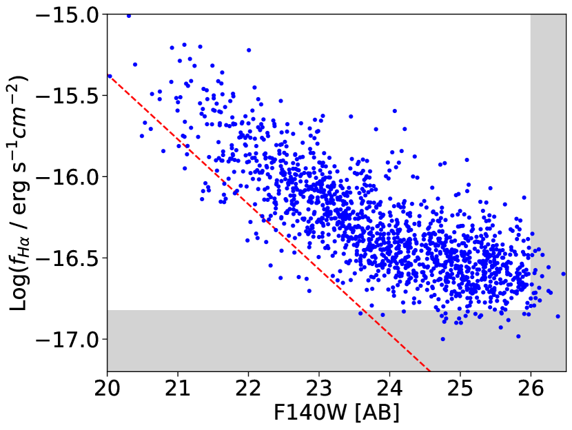
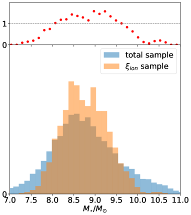
Figure 1: Completeness estimate of the sample selection. Left: H$\alpha$ flux as a function of magnitude in the NIR F140W band for the galaxy sample selected for this study. The red dashed line represents $EW_{\mathrm{H}\alpha}$= 80 Å, the observed equivalent width cut used in our selection. The gray-shaded areas denote the H$\alpha$ flux limit of $1.5\times 10^{-17}$ erg s^-1 cm^-2 and the magnitude limit of F140W images at $AB=26$ mag. Right: stellar mass distribution for the entire spectroscopic sample (in blue) and the selected sample (in orange). Both distributions are re-normalized. The top panel shows the ratio of the relative fractions of both samples. It shows a significant decrease in the completeness at the low (M_⋆$\sim 10^{8}$ M_⊙) and high (M_⋆$\sim 10^{9.5}$ M_⊙) stellar mass. Stellar masses are part of the 3D-HST data release and were originally estimated by Skelton et al. (2014).

The combination of the grism spectroscopy and the UV imaging provides us with the opportunity to explore the star formation activity on different timescales and measure the ionizing efficiency of star forming galaxies at $z\sim 1$ as a function of their physical parameters. We have selected our sample based on high-significance H$\alpha$ emission lines (above SNR=3) and equivalent widths higher than 80 Å in the spectroscopic data, and SNR$>3$ continuum detection in the F336W filter of the UV data. The final sample contains a total of 1167 objects in the redshift range $0.7<z<1.5$.

The NIR grism spectroscopy is particularly sensitive to strong nebular emission lines. Most of the objects in this sample will have relatively high equivalent widths, and in some cases, their continuum will remain undetected. Therefore, equivalent width measurements will be highly uncertain. We have re-computed the equivalent width of all the emission lines using the line flux and the broadband magnitude in the $JH_{140}$ images, correcting for the contribution of line flux to the observed magnitudes:

$$EW_{cor}=\frac{F_{line}}{f_{\lambda,140}-\frac{\int f_{\lambda,line}d\lambda}{\int d\lambda}}$$ (1)

where $f_{line}$ is the line flux and $f_{\lambda,140}$ is the flux density in the F140W filter. While continuum-selected samples are limited by the depth of the imaging data, our emission-line selection favors high equivalent width galaxies showing enough contrast between the line and the continuum. The left panel of Figure 1 shows the impact of this selection on the completeness in H$\alpha$ flux as a function of magnitude. While the faint-end limits of both continuum and line fluxes are represented by the shaded area, the line flux limit increases towards brighter magnitudes. Beyond a magnitude $JH\sim 24$, the sample is defined not only by the equivalent width, but also by the H$\alpha$ flux limit. For these faint galaxies, we will only select bright H$\alpha$ emitters relative to their continuum magnitude. This impact of this selection bias will be in Section 4. Comparing the stellar mass distribution for the H$\alpha$ sample and the parent sample, we can see on the right panel of Figure 1 that the selected sample becomes incomplete towards low stellar masses, typically around Log(M_⋆/M_⊙$=8$), and at high masses around Log(M_⋆/M_⊙$=9.5$). This is due to our sample selection, which is based on SNR cuts on both H$\alpha$ and UV emission, on one hand, and EW(H$\alpha$), on the other hand.

3.1 Dust attenuation correction

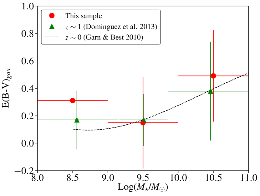
Figure 2: Nebular attenuation as a function of the stellar mass. The reddening E(B-V)_gas is computed using the Balmer decrement of a subsample of galaxies binned in stellar mass. Our data points (red circles) are plotted together with the results of Domínguez et al. (2013) (green triangles). The dashed line represents the relation derived for local galaxies by Garn & Best (2010).

To correct the parameter measurements for dust attenuation, we consider the H$\alpha$ and UV continuum emission independently. First, we compute the nebular attenuation from the Balmer decrement H$\alpha$/H$\beta$ for a subsample of 10 galaxies over a restricted redshift range of $1.3<z<1.51$, where both H$\alpha$ and H$\beta$ lines are visible in the G141 grism, and we examine the trends as a function of stellar mass and H$\alpha$ luminosity. Figure 2 shows a good agreement with the results of Domínguez et al. (2013) who used a stack of $0.75<z<1.5$ emission-line spectra to derive Balmer decrements as a function of stellar mass. It also follows the trend derived for local galaxies (Brinchmann et al., 2004; Garn & Best, 2010) with no sign of evolution with redshift, which was also observed at $z>1$ (e.g. Sobral et al., 2012; Domínguez et al., 2013). We apply the relation derived by Domínguez et al. (2013) to the entire galaxy sample to estimate the nebular attenuation.

As for the UV luminosity, we compute the UV slope over a rest-frame spectral range of $1300-3300$ Å by performing a multi-band fitting to the relation $f_{\lambda}\propto\lambda^{\beta}$. Then we derive the attenuation by adopting an intrinsic UV slope of $\beta_{0}=-2.62$ (Reddy et al., 2018a). The intrinsic UV slope is sensitive to the star formation history (SFH) of galaxies, which in turns affects the computed stellar attenuation. Galaxies with higher specific star formation rate have bluer UV colors due to a lower contribution of older stellar populations. The present sample has relatively high sSFRs and strong emission lines, with median values of sSFR=$10^{-8.4}$ yr^-1 and EW_rest(H$\alpha$)=160 Å (cf. Fig. 4). We show in Appendix C the effects of adopting the standard value of $\beta_{0}=-2.23$ of Meurer et al. (1999).

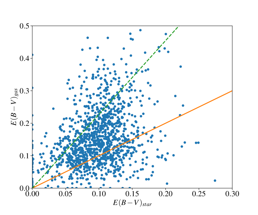
Figure 3: The nebular dust reddening vs the stellar dust reddening. The reddening values are computed using the main combination of dust laws: the Cardelli et al. (1989) attenuation law for $E_{B-V,\mathrm{gas}}$ and the SMC extinction law for $E_{B-V,\mathrm{stars}}$. The solid orange line denotes the 1:1 relation, while the dashed blue line marks the Calzetti et al. (2000) relation $E_{B-V,\mathrm{stars}}$= 0.44$E_{B-V,\mathrm{gas}}$.

Emission	Curve	E(B-V)	Correction Factor
H$\alpha$	Cardelli	0.14	1.40
H$\alpha$	Calzetti	0.12	1.50
UV	SMC	0.10	3.3
UV	Calzetti	0.23	11.3

Table 1: The importance of dust correction for the H$\alpha$ and UV emissions. We list the reddening estimates and the correction factors for the different extinction/attenuation laws considered in this work.The E(B-V) values represent the nebular and the stellar reddening for the H$\alpha$ and UV fluxes, respectively

.

Many efforts have been undertaken to investigate the attenuation law in high-redshift galaxies. There has been some evidence for a different calibration compared to local galaxies, possibly due to their younger age, lower metallicities or their different emission line properties in general (de Barros et al., 2014; Price et al., 2014; Reddy et al., 2015; Smit et al., 2016; Cowie et al., 2016). In Section 4 we adopt the Cardelli et al. (1989) curve for H$\alpha$ emission and the SMC extinction curve (Gordon et al., 2003) for the UV continuum. When computing absolute values such as the ionizing efficiency (Section 5) we explore the effects of adopting two laws for the nebular attenuation, namely the Calzetti et al. (2000) and Cardelli et al. (1989) curves. Regarding the stellar continuum, we also compare the SMC extinction curve (Gordon et al., 2003) with the Calzetti et al. (2000) attenuation curve in computing E(B-V)_s, keeping the same intrinsic slope $\beta_{0}=-2.62$. Table 1 shows the resulting correcting factors for H$\alpha$ and UV luminosities when adopting different dust laws. We also show in Figure 3 the relation between $E_{B-V,\mathrm{gas}}$ and $E_{B-V,\mathrm{stars}}$. An important dispersion is observed, with most of the sample lying between the 1:1 ratio and the 0.44 factor of Calzetti et al. (2000).

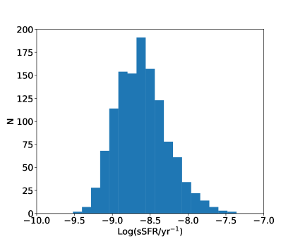
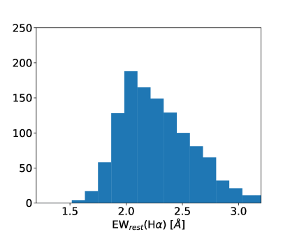
Figure 4: Left: specific star formation rate distribution from our sample, computed from the H$\alpha$ emission following Kennicutt & Evans (2012) calibration and corrected for dust attenuation using the Cardelli et al. (1989) law. Right: distribution of the H$\alpha$ equivalent width calculated in the rest frame.

4 Star Formation Burstiness in low-mass galaxies

While star formation is expected to proceed smoothly in massive galaxies, it becomes highly stochastic in lower mass galaxies, with short-lived intense bursts of star formation. These bursts are marked by high H$\alpha$ equivalent but also high $\xi_{\mathrm{ion}}$ as shown by hydrodynamical simulations (Shen et al., 2014; Domínguez et al., 2015). In this section, we will explore the effects of star formation burstiness on the galaxy observables.

4.1 SFR-M_⋆ relation

Observations from the local universe to high-redshift galaxies show a tight correlation between the star formation rate and stellar mass (e.g. Brinchmann et al., 2004; Noeske et al., 2007; Whitaker et al., 2014). The underlying picture is that galaxies accrete gas and build up their stellar mass in a gradual and smooth process, with constant SFR averaged over hundreds of Myrs. However, during the last decade, observations of low-mass galaxies, primarily selected upon their strong emission lines, have painted a different picture of star formation processes. In particular, extreme emission line galaxies (EELGs) experience short episodes of intense star formation, leading to excursions from the SFR-M_⋆ main sequence (Weisz et al., 2012; Atek et al., 2014; Guo et al., 2016; Faisst et al., 2019; Emami et al., 2019), although, the averaged SFR over cosmic time, would match a steady star formation scenario. Several hydrodynamical simulations also unveiled the stochastic processes at play in low-mass galaxies compared to their massive counterparts (Shen et al., 2014; Domínguez et al., 2015; Sparre et al., 2017), as a result of episodes of gas accretion that trigger star formation followed by stellar feedback and gas outflows, which hampers gas infall into the galaxy.

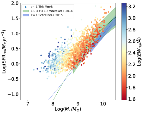
Figure 5: The star formation rate as function of stellar mass, known as the star formation main sequence. SFR(H$\alpha$) is corrected for dust attenuation using the Cardelli law. Our data points are also colored according to their H$\alpha$ equivalent width. The green solid line and the blue dashed line show the results of Whitaker et al. (2014) for $1<z<1.5$ galaxies and the relation derived by Schreiber et al. (2015) at $z=1$, respectively. the shaded areas are the associated uncertainties, while the dot-dashed lines represent an extrapolation of the above-mentioned relations below their stellar mass limits.

We first use the H$\alpha$ emission to compute the SFR following the Kennicutt & Evans (2012) calibration, assuming a solar metallicity and a Chabrier (2003) IMF, and a Cardelli dust attenuation correction. The SED fitting procedure used to constrain the stellar mass also assumes a Chabrier IMF (Skelton et al., 2014). In Figure 5, we plot the correlation between the SFR and M_⋆ for our sample of galaxies together with the best-fit relations in the literature at similar redshifts, which combined the observed UV and reprocessed IR light to derive the total SFR. Whitaker et al. (2014) derived the total IR luminosity using a luminosity-independent conversion factor from the Spitzer/MIPS 24 $\mu$m based on a single SED template (Wuyts et al., 2011a). Schreiber et al. (2015) compute the total IR luminosity by fitting SED templates from Chary & Elbaz (2001) to the Herschel flux densities and measure L_IR in the best-fit template. A significant fraction of the sample lies above the main sequence relations. We can see that the departure from the main sequence is associated with an increase in $EW_{\mathrm{H}\alpha}$. In fact, only galaxies with $EW_{\mathrm{H}\alpha}$ around a hundred Å follow the main sequence. AS explained earlier, this is the result of the elevated instantaneous SFR, probed by H$\alpha$, following a recent burst of star formation. The observed flattening of the slope towards low-mass galaxies is likely the result of H$\alpha$ flux incompleteness, as we reach SFRs below 1 M_⊙ yr^-1. However, it is clear that the deviation from the main sequence is much larger at low mass, as the highest $EW_{\mathrm{H}\alpha}$ values are observed at lower masses.

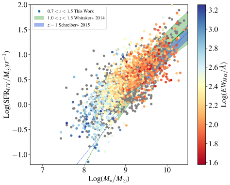
Figure 6: The star formation rate as derived from the UV (SFR_UV) as a function of the stellar mass. The colored points are the same as in Figure 5, except the SFR is derived from the UV emission and corrected for dust extinction using the SMC law. In addition, the gray points represent the total SFR, which is the sum of the uncorrected SFR_UV and the SFR_IR (Skelton et al., 2014).

Regardless of the SFR limit, the scatter seems to increase towards lower masses, indicating a higher stochasticity in star formation histories. In order to quantify the apparent increase of the scatter towards lower-galaxies, we populated the SFR-M_⋆ plane with simulated galaxies following the MS relation of Whitaker et al. (2014) with the corresponding scatter. Then we applied a similar H$\alpha$ flux selection used in the observations. We can see the results in Fig. 7. The blue points follow the expected MS trend, but below a stellar mass of Log(M_⋆/M_⊙)$\sim 9$, the H$\alpha$ flux selection removes most of the galaxies (represented by light blue points). The corresponding completeness limit in SFR(H$\alpha$) is indicated by the gray shaded region. In our observations, we are still detecting a significant fraction of galaxies (red points) below Log(M_⋆/M_⊙)$\sim 9$, most probably because of an increased scatter towards lower masses. A good agreement between the simulations and observations in the mass range below Log(M_⋆/M_⊙)$\sim 9$ is achieved by using a scatter a factor of 3 higher than the one observed at higher masses. This stands in contrast with other studies based on UV-selected samples or SED-based SFR indicators, who found no evidence of increasing scatter towards lower masses (Kurczynski et al., 2016), nor evidence for an enhanced H$\alpha$ luminosity compared to UV (Guo et al., 2016). Boogaard et al. (2018) also explored the low-mass end of the main sequence at $0.1<z<0.9$ by using Balmer lines to measure the SFR, finding an intrinsic scatter similar to Kurczynski et al. (2016) and a shallower slope compared to massive galaxy samples.

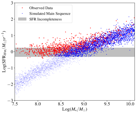
Figure 7: The evolution of the scatter in the SFR-M relation. The blue points represent simulated galaxies following the Main Sequence relation and scatter of Whitaker et al. (2014). The light-blue points are the galaxies excluded by the H$\alpha$ flux selection used in our observations. The gray shaded area represents the SFR_Hα limit in the redshift range of our sample. The red points are the observed galaxies shown in Fig. 5.

In Figure 6, we show how our sample fits in the main sequence diagram when the SFR is derived from the UV. When compared to Figure 5, the galaxies follow more closely the MS, although these relations are extrapolated here (dashed lines) at lower masses (mainly below $10^{9}$ M_⊙). This follows the scenario where, recent star formation traced by H$\alpha$, likely causes the excursion of galaxies out of the MS. In the same figure, we also compare the dust-corrected SFR_UV with the total SFR (represented by gray points), which was estimated by adding up the uncorrected SFR_UV and the SFR_IR derived from the IR luminosity at $8-1000$ $\mu$m measured from Spitzer/MIPS 24 $\mu$m photometry (Skelton et al., 2014). Although about 20% of the sample is missing because they are not detected in the Spitzer data, we can see the dust corrected SFR is globally in fair agreement with the total SFR.

4.2 H$\alpha$ and UV SFR indicators

The ratio between SFR_Hα and SFR_UV is often used an indicator of star formation burstiness in galaxies (e.g., Meurer et al., 2009; Weisz et al., 2012; Guo et al., 2016; Broussard et al., 2019). At the onset of a burst, the H$\alpha$ flux increases over a very short timescale of $\sim 10$ Myr, whereas UV bright and less massive stars will run on a longer period $\sim 100$ Myr) (e.g. Leitherer et al., 1999; Hao et al., 2011; Kennicutt & Evans, 2012; Calzetti, 2013). Therefore, important variations in SFR_Hα/SFR_UV ratio are expected when the star formation is non-steady and out of equilibrium. For instance, Weisz et al. (2012) produced a set of SFH history models to match the observations of a sample of local galaxies. They find that low-mass galaxies experience a bursty star formation, with burst episodes lasting less than 10 Myr and a period of 250 Myr between bursts. Those models appear to reproduce the observed variations of the $f(H\alpha)/f(UV)$ ratio, which are mostly below unity. Emami et al. (2019) improved this analysis with a larger parameter space with exponentially rising and declining SFH and find similar results, albeit with a larger burst duration. In their analysis, they explore the star formation burstiness by comparing the $L(H\alpha)/L(UV)$ with $\Delta L(H\alpha)$, which are correlated, in particular at lower stellar masses. The bursty nature of star formation in low-mass galaxies has been confirmed by hydrodynamical simulations. In the FIRE simulations, Sparre et al. (2017) show that the SFR probed on a short timescale by H$\alpha$ can vary by an order of magnitude compared to the UV indicator. They also find a significant fraction of galaxies with SFR_Hα/SFR_UV ratios well below unity.

In general, the explanation for the decline of the SFR_Hα/SFR_UV ratio observed in those studies is based on the different timescales of these emissions. At the onset of the burst, the H$\alpha$ emission is brighter than the FUV. The stars responsible for the FUV emission have a longer lifetime. This means that the FUV emission will gradually take over, and the SFR_Hα/SFR_UV will decline steadily below unity over the course of the burst in the first $\sim 50$ Myr. After the end of the burst, the H$\alpha$ emission from massive stars becomes negligible, as the stars responsible for this emission die after $\sim 10$ Myr. Over the next $100-200$ Myr, the FUV emission in turn starts to fade, as the less massive stars start to disappear, leading to a steady increase in the SFR_Hα/SFR_UV ratio. Around $300$ Myr, the SFR_Hα/SFR_UV returns to its equilibrium value of unity, which marks the end of the burst cycle (Weisz et al., 2012; Domínguez et al., 2015; Emami et al., 2019). According to this scenario, the observed SFR_Hα/SFR_UV ratio is below unity during most of the burst cycle.

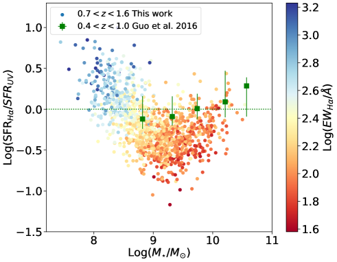
Figure 8: The ratio of H$\alpha$ and UV SFR indicators as a function of stellar mass. SFR_Hα is corrected for dust attenuation using the Cardelli law and SFR_UV with the SMC curve. Data points are also color-coded with $EW_{\mathrm{H}\alpha}$. The horizontal line indicates a one-to-one ratio. The results of Guo et al. (2016) are show with green squares. Note that these points represent the ratio SFR_Hβ/SFR_UV.

In Figure 8, we plot the SFR_Hα/SFR_UV ratio as a function of stellar mass for our sample, assuming an SMC dust correction for the UV continuum. At high masses ($>10^{9}$M_⊙), the ratio of SFR indicators is mainly close or below unity. For galaxies with M_⋆ $<10^{9}$M_⊙, the ratio is around unity or higher. From the same figure, we can see a similar trend with $EW_{\mathrm{H}\alpha}$, as galaxies with $EW_{\mathrm{H}\alpha}$ of a few hundreds to a thousand Å are the ones with higher SFR ratios. The main result is that we observe an SFR_Hα/SFR_UV ratio above unity mainly in low-mass galaxies (M_⋆ $<10^{9}$M_⊙) rather than in more massive galaxies (M_⋆ $>10^{9}$M_⊙). This result is different from what is observed in the studies mentioned earlier and the associated scenario, where SFR_Hα/SFR_UV is observed to be mainly below unity. Of course, because of our H$\alpha$ flux selection (see Section 3 and Figure 7), we might be missing SFR_Hα/SFR_UV lower than unity at M_⋆ $<10^{9}$M_⊙. However, the observation of elevated SFR_Hα/SFR_UV in low-mass galaxies still stands, and is not observed in more massive galaxies.

For comparison, the other notable studies along these findings are Shim et al. (2011) and Faisst et al. (2019) who analyze a sample of $z\sim 4$ galaxies for which they measure H$\alpha$ through the IRAC 3.6$\mu$m excess. Shim et al. (2011) find an SFR ratio of SFR_Hα/SFR_UV $=6.1\pm 4.1$, even higher than our result. Not surprisingly, their sample also has a very high H$\alpha$ equivalent width distribution ($EW_{\mathrm{H}\alpha}$= 140-1700 Å), due to the IRAC selection, which is sensitive to H$\alpha$ emitters with $EW_{\mathrm{H}\alpha}$ higher than 70-350 Å. This effect is clearly visible in Fig. 8, where high-$EW_{\mathrm{H}\alpha}$ galaxies have the highest SFR_Hα/SFR_UV. Similarly, Faisst et al. (2019) find that more than 50% of their sample has SFR_Hα in excess compared to SFR_UV, particularly in low-mass galaxies. They also find an anti-correlation between $EW_{\mathrm{H}\alpha}$ and stellar mass. The trend and SFR ratios observed at low masses differ from the results of some previous studies summarized above (Weisz et al., 2012; Sparre et al., 2017). This was already observed in Figure 5 where the scatter of the main sequence (i.e. $\Delta L(H\alpha)$) is larger at lower masses. We note that Emami et al. (2019) also find a larger scatter int the L(H$\alpha$) vs M_⋆ relation towards lower mass galaxies.

Given the timescales traced by H$\alpha$ and UV, the distribution of SFR_Hα/SFR_UV and its dispersion provides an indication on the SFH parameters. As discussed earlier, since SFR_UV runs on hundreds Myr, while SFR_Hα on 10 Myr, the distribution of observed galaxies should be centered on the low side of SFR_Hα/SFR_UV. However, a variation in the following two parameters will increase the prevalence of galaxies with higher SFR ratios like the ones observed here: (i) a larger $\tau$ in the exponential SF; or (ii) a higher duty cycle, i.e. a shorter period between successive SF bursts.

In this context, the results of Guo et al. (2016) are also shown in Fig. 5. They selected a sample of 165 galaxies at $0.4<z<1$ with SNR(H$\beta$)$>3$ and SNR(F275W)$>5$. They derived SFR_Hα using the H$\beta$ flux, the case B recombination ratio of 2.86, and the calibration of Kennicutt & Evans (2012). They derived SFR_UV using the UV luminosity at 1500 Å and the same calibration of Kennicutt & Evans (2012). Both determinations assume a Chabrier IMF and solar metallicity. We used the same calibration and parameters to derive the SFRs of the present sample. Guo et al. (2016) also showed that dust correction is negligible for these SFR determinations and apply a correction only for galaxies with SFR_UV+IR/SFR${}_{1500A}>20$. They do not find the mass-dependant trend observed in our sample, but rather an increase in the SFR ratio with increasing mass. Again, it is possible that these differences are partially due to selection effects, since their sample has a median $EW_{H\beta}=15$ Å, a factor of two lower than our sample. We argue that if this were only due to selection effects, these high-EW lines should also be present in higher-mass systems. Our sample most likely probes a low-mass galaxy population caught during a burst of star formation, rather than its decline as seen in those studies. Theoretical models of bursty star formation also predict an increase of this mode in low-mass galaxies (e.g. Faucher-Giguère, 2018) due to shorter dynamical timescales and probably higher gas fractions.

Another possible source for the variations in the SFR_Hα/SFR_UV ratio in low-mass galaxies is a stochastic sampling of the IMF. In the case of low-mass galaxies with a low SFR, massive stars could form less frequently than assumed, leading to deviations of SFR_Hα/SFR_UV from equilibrium even in the case of a steady star formation. Numerous studies have explored the effects on IMF sampling (Pflamm-Altenburg et al., 2009; Fumagalli et al., 2011; Weisz et al., 2012; Guo et al., 2016; Emami et al., 2019). Overall, the resulting variations in SFR indicators were insufficient to reproduce the observed decline of SFR_Hα/SFR_UV. The discrepancy is even larger for our results, where we observe a clear increase towards lower masses, which makes the IMF sampling an unlikely scenario.

Finally, several uncertainties remain regarding the determination of the SFR_Hα/SFR_UV ratio and its evolution as a function of galaxy parameters. Both SFR indicators use conversion factors from H$\alpha$ and UV luminosities assuming a constant star formation. Of course, we expect important deviations from these assumptions for different SFHs, particularly in the case of bursty star formation. If both SFR calibrations were correct, we would expect the SFR_Hα and SFR_UV to be equal. This is precisely why such a ratio can reveal deviations from steady star formation scenarios and trace bursty SFH. In addition to SFH, the inclusion of binary stars in stellar population models and a higher mass end (300 M_⊙) for the IMF (Wilkins et al., 2019) can increase SFR_UV by 0.15-0.2 dex, and SFR_Hα by 0.35 dex. Castellano et al. (2014) also showed that SFR_UV tend to underestimate the true SFR of $z\sim 3$ Lyman break galaxies with sub-solar metallicity by a factor of a few. It is unclear whether this underestimate would also apply to lower-mass galaxies at lower redshifts. Furthermore, if the attenuation curve for the stellar continuum is different in lower-mass galaxies (e.g., Salim & Narayanan, 2020), it will also affect the SFR ratio. One scenario that would contribute to the increase of SFR_Hα/SFR_UV ratio towards lower mass galaxies is the one where the dust attenuation law becomes steeper towards low-mass galaxies.

5 ionizing efficiency

We compute the ionizing efficiency $\xi_{\mathrm{ion}}$, which is defined as the ratio between the ionizing (Lyman continuum) photon production $\dot{N}_{\mathrm{ion}}$ and the observed non-ionizing UV luminosity density $L_{\rm UV}$ estimated at 1500 Å:

$$\xi_{\rm ion}=\frac{\dot{N}_{\rm ion}}{L_{UV}}~{}[erg^{-1}~{}Hz]$$ (2)

In the framework of the case B recombination theory (Osterbrock, 1989), $\dot{N}_{\rm ion}$ can be estimated from Hydrogen recombination lines (Leitherer & Heckman, 1995):

$$L(H\alpha)~{}[erg~{}s^{-1}]=1.36\times(1-f_{esc})~{}10^{-12}~{}{\dot{N}_{\rm ion}}~{}[s^{-1}]$$ (3)

where $L(H\alpha)$ is the H$\alpha$ luminosity and $f_{esc}$ is the escape fraction of Lyman continuum radiation from galaxies. Most results in the literature indicate a wide range of $f_{esc}$ values, both in low- and intermediate- redshift galaxies. Recent spectroscopic measurements in $z\sim 0.3$ compact star-forming galaxies reported by Izotov et al. (2016, 2018) indicate an escape fraction between 2 and 70%. Imaging campaigns at higher redshifts reported a few robust detections with escape fraction exceeding $f_{esc}$ $\sim 50\%$ (e.g., Shapley et al., 2016; Vanzella et al., 2016; Bian et al., 2017; Vanzella et al., 2018; Rivera-Thorsen et al., 2019). On the other hand, Rutkowski et al. (2017) estimate an upper limit of $f_{esc}$ $<15$ % in emission-line galaxies at $z\sim 2.5$, using partly the 3DHST G141-grism data in GOODS-N and UVUDF fields. For the sake of consistency with literature results, here we assume a zero escape fraction of LyC radiation. Accounting for $f_{esc}$(LyC) will result in a higher $\xi_{\mathrm{ion}}$.

According to equations 2 and 3, $\xi_{\mathrm{ion}}$ is equivalent to the ratio SFR_Hα/SFR_UV, modulo a factor of $1.3\times 10^{26}~{}(1-f_{esc})$. Therefore, in the case where we assume a zero escape fraction, this burstiness indicator is a direct probe of the ionizing efficiency and its evolution with galaxy parameters. The ionizing efficiency will be subject to the same uncertainties discussed earlier for the SFR ratio.

In Figure 9, we demonstrate how our sample selection translates into $\xi_{\mathrm{ion}}$ completeness. We plot the H$\alpha$ luminosity as a function of UV luminosity for our $\xi_{\mathrm{ion}}$ sample, together with their respective limits (gray shaded regions) derived from the depth of the observations. Combining the $EW_{\mathrm{H}\alpha}$ cut and H$\alpha$ flux limit, and using the observed correlation between the UV and IR magnitude, we computed the $\xi_{\mathrm{ion}}$ limit (red-shaded area), assuming a redshift range of $0.7<z<1.5$ in the simulations (cf. Appendix A). Overall, these simulations will be helpful in assessing the limits of the correlations we explore in Section 6.

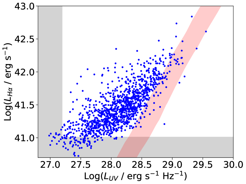
Figure 9: The H$\alpha$ luminosity as a function of rest-frame UV luminosity for the $\xi_{\mathrm{ion}}$ sample. The red-shaded region represents the $\xi_{\mathrm{ion}}$ lower limit imposed by our equivalent width cut (cf. Figure 1). The associated range of values account for the redshift range $0.7<z<1.5$ and the relationship between the IR and UV magnitudes (cf. text for details). Shaded regions along both axes indicate the detection limits in L(H$\alpha$) and L(UV), calculated at the mean redshift of the sample.

5.1 Ionizing efficiency results

The results of the dust-corrected estimates of $\xi_{\mathrm{ion}}$ are shown in Figure 10. Adopting standard attenuation corrections using the Cardelli et al. (1989) law for H$\alpha$ emission and the SMC curve for UV continuum, we obtain a median ionizing efficiency of Log($\xi_{\mathrm{ion}}$/erg^-1 Hz)$=24.80\pm 0.26$. Adopting the Calzetti law for the nebular attenuation has little effect on the ionizing efficiency, except when deriving the nebular attenuation by applying a factor of 1/0.44 to the stellar attenuation (Calzetti et al., 2000). The $\xi_{\mathrm{ion}}$ estimates are more sensitive to the attenuation curve in the UV domain. The derived $\xi_{\mathrm{ion}}$ are lower by 0.45 dex if we assume the Calzetti attenuation curve rather than the SMC curve for dust-correcting the UV luminosity density. The scatter in the $\xi_{\mathrm{ion}}$ distribution increases by 0.11 dex in this case. Table 1 summarizes the relative importance of dust correction to the H$\alpha$ and UV emissions. We can see that the correction factor applied to the UV emission is much larger than the one for H$\alpha$. Also, the choice of an attenuation law is more critical for the UV emission. In figure 11, we show the $\xi_{\mathrm{ion}}$ distribution in four mass bins to highlight the dependence on stellar mass discussed later in Section 6.

Figure 10: Distribution of the ionizing efficiency $\xi_{\mathrm{ion}}$. The blue, orange, green, and red histograms show the dust-corrected measurements using three different combinations of attenuation curves for the nebular emission and the UV continuum: Cardelli et al. (1989)/SMC, Calzetti et al. (2000)/Calzetti et al. (2000) but assuming the nebular attenuation is a factor of (1/0.44) higher than the stellar attenuation, Calzetti et al. (2000)/SMC, and Cardelli et al. (1989)/Calzetti et al. (2000) curves, respectively. The main combination used in Section 4 yields the green distribution. The median values for each configuration are Log($\xi_{\mathrm{ion}}$/erg^-1 Hz)$=24.80\pm 0.26$, $24.93\pm 0.24$, $24.83\pm 0.27$, $24.26\pm 0.36$.

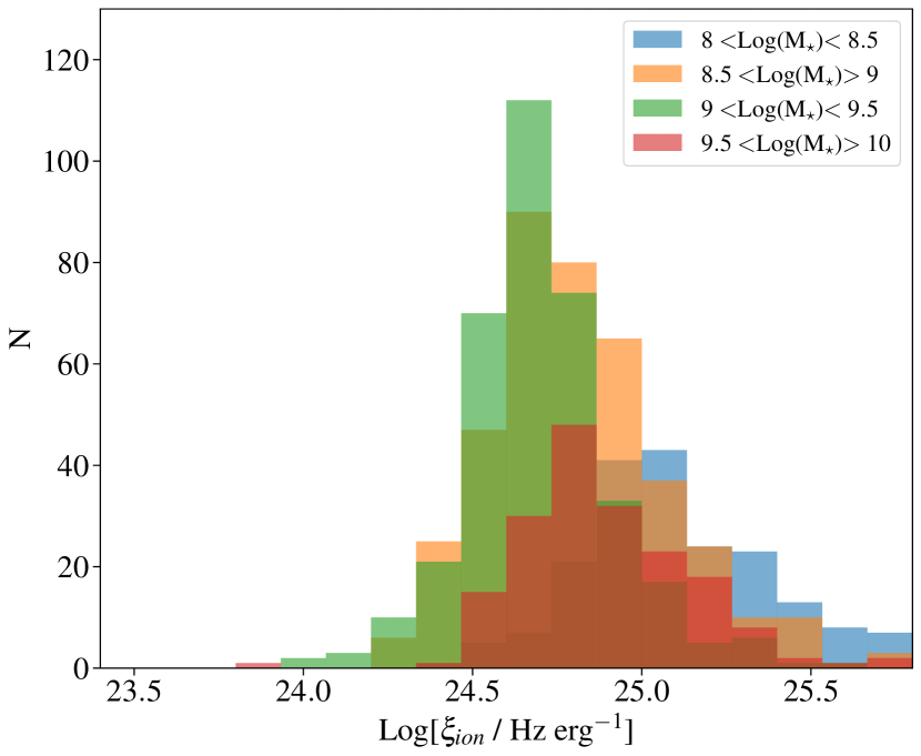
Figure 11: The $\xi_{\mathrm{ion}}$ distribution in four different bins of stellar mass. The Cardelli/SMC combination is adopted for dust correction.

These values are in general significantly lower than what has been found in previous studies and the canonical value of Log($\xi_{\mathrm{ion}}$)$=25.2$ widely used in computing the ionizing budget of galaxies (e.g., Robertson et al., 2013). As a comparison, Emami et al. (2020) report an average Log($\xi_{\mathrm{ion}}$)$=25.47\pm 0.09$ in a sample of lensed galaxies at $z\sim 2$, which is almost an order of magnitude higher. At a similar redshift, Shivaei et al. (2018) find Log($\xi_{\mathrm{ion}}$)$=25.34$. Both values are derived with an SMC extinction correction of the UV luminosity.

We list below a literature compilation of $\xi_{\mathrm{ion}}$ determinations at different redshifts.

• The results of Emami et al. (2020) are based on spectroscopic observations of 28 $z\sim 2$ lensed galaxies, with a similar stellar mass range probed by our sample ($8\leq Log(M_{\star}/M_{\odot})\leq 10$). The study follows the same approach used here for $\xi_{\mathrm{ion}}$ estimates and dust correction. However, their results are based on stacked spectra, in bins of physical properties (stellar mass, UV magnitude, UV continuum slope).

• Shivaei et al. (2018) used spectroscopic and UV imaging data from the MOSDEF survey to measure $\xi_{\mathrm{ion}}$ in a large sample of 673 galaxies at $1.4<z<2.6$. They use the Balmer decrement H$\alpha$/H$\beta$ to measure nebular attenuation, whereas it is available for only a sub-sample of our galaxies (cf. Section 3.1). Stellar attenuation is derived from SED fitting. Importantly, that work probes stellar masses above $Log(M_{\star}/M_{\odot})>9$, which is significantly higher than the present sample.

• Using spectroscopic observations to measure H$\beta$ emission and SED fitting to infer the UV continuum emission, Nakajima et al. (2016) measured $\xi_{\mathrm{ion}}$ in sample of 15 Ly$\alpha$ Emitters and Lyman Break Galaxies at $z\sim 3$. No dust attenuation was assumed in this determination. We computed an average $\xi_{\mathrm{ion}}$ in a sub-sample of $Log(M_{\star}/M_{\odot})\sim 9.7$ galaxies. Their sample also include galaxies with no H$\beta$ detection and whose $\xi_{\mathrm{ion}}$ upper limits and stellar masses are lower than the average values reported in the Figure.

• Unlike these studies, Matthee et al. (2017) used narrowband observations to measure the H$\alpha$ flux and infer $\xi_{\mathrm{ion}}$ in a sample of $z\sim 2.2$ galaxies. We select here their low-mass sample of H$\alpha$ emitters with an average stellar mass of Log($M_{\star}/M_{\odot})\sim 9.2$).

• In addition, several studies have used the broad-band excess between the $3.6\mu m$ and $4.5\mu m$ Spitzer/IRAC channels to derive the H$\alpha$ flux of $z>4$ galaxies. Based on this method, Bouwens et al. (2016) derived $\xi_{\mathrm{ion}}$ for galaxies at $z\sim 4.4$ and $z\sim 5.25$. These values were corrected for dust using a stellar attenuation derived from SED fitting. The results of two attenuation laws (Calzetti and SMC) are shown in the Figure. Their stellar mass range is also comparable to this work, with an average value around Log($M_{\star}/M_{\odot})\sim 9$).

• Similarly, Lam et al. (2019) used stacked IRAC colors to measure H$\alpha$ emission and infer $\xi_{\mathrm{ion}}$ in sample of 300 galaxies at $3.8<z<5.3$ with spectroscopic redshifts. The dust correction is based on UV continuum slope measurements and the SMC curve. We here report the average $\xi_{\mathrm{ion}}$ value computed in sub-sample over a stellar mass range of $8\leq Log(M_{\star}/M_{\odot})\leq 10$.

• At higher redshifts, Stark et al. (2015) obtained rest-frame UV spectroscopy of $z\sim 7$ lensed galaxies and used stellar population and photo-ionization models to infer the ionizing efficiency of one of them. As the authors note, the intense radiation field of this galaxy is not necessarily representative of the galaxy population at $z>6$ because of the strong equivalent width selection and the bright Ly$\alpha$ emission.

Within this list of studies, only Emami et al. (2020) has both spectroscopic measurements of the H$\alpha$ flux and UV imaging to accurately infer $\xi_{\mathrm{ion}}$ for galaxies in the same range of stellar mass as probed in this study. The main differences are the lower redshift range and the much larger sample size used in the present study. In figure 12, we keep only the studies that probe a similar stellar mass range and use the same dust prescriptions as our study. We observe a clear evolution of $\xi_{\mathrm{ion}}$ as a function of lookback time $t_{L}$, ranging from Log($\xi_{\mathrm{ion}}$)$=24.70$ at $t_{L}\sim 8.3$ Gyr to Log($\xi_{\mathrm{ion}}$)$=25.54$ at $t_{L}\sim 12.7$ Gyr. We perform a linear fit to all the data points by computing the maximum likelihood using Markov Chain Monte Carlo (MCMC) simulations using emcee (Foreman-Mackey et al., 2013). In Figure 12, we plot the best-fit relation and 95% confidence interval of the fit. We find a best-fit relation of Log($\xi_{\mathrm{ion}}$) $=0.21~{}t_{L}+22.82$. Such evolution is expected since galaxy physical properties are known to evolve with redshift. For instance, the emission-line selection naturally favors high equivalent widths for the H$\alpha$ line and the average H$\alpha$ equivalent width of emission-line galaxies is known to increase with redshift (e.g., Atek et al., 2011; Smit et al., 2014; Faisst et al., 2016; Reddy et al., 2018a). These effects can explain the higher $\xi_{\mathrm{ion}}$ values observed at higher redshifts (see also Section 6).

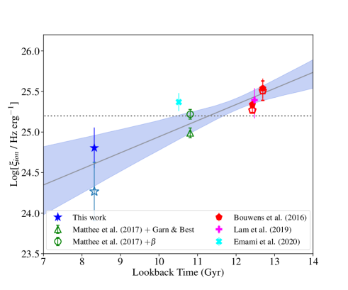
Figure 12: The ionizing efficiency as a function of lookback time. Our measurement at $z\sim 1$ (blue stars) are compared with literature results at higher redshifts. Note that the median stellar mass of our sample is comparable to the other studies on this figure (see text for details). The filled (open) symbols show the difference in $\xi_{\mathrm{ion}}$ measurements when an SMC (Calzetti) curve is used to correct or dust. The dotted horizontal line indicates the canonical value of Log($\xi_{\mathrm{ion}}$)$=25.20$. The gray line and the shaded area show our best-fit results and associated 95% confidence interval. The fit is performed on all the data points shown here.

6 Evolution of $\xi_{\mathrm{ion}}$ with galaxy properties

We now explore the evolution of $\xi_{\mathrm{ion}}$ as a function of the galaxy physical properties.

6.1 The relation between $\xi_{\mathrm{ion}}$ and $EW_{\mathrm{H}\alpha}$

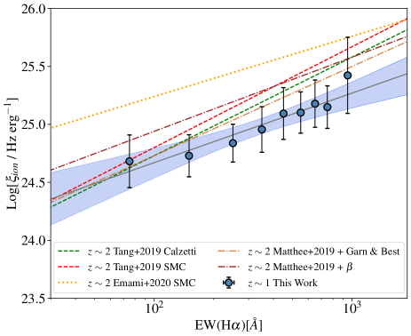
Figure 13: The ionizing efficiency as a function of H$\alpha$ line equivalent width (blue circles). Error bars indicate the dispersion in each $EW_{\mathrm{H}\alpha}$ bin. The best-fit relation is shown with a gray solid line with associated 68% confidence interval (shaded area). Other correlations found at higher redshift in the literature are also shown: orange dotted line for Emami et al. (2020), green and red dashed lines for Tang et al. (2019), orange and brown dot-dashed lines for Matthee et al. (2017). The legend also indicates the prescriptions used for dust corrections in each study.

As previously noted, $\xi_{\mathrm{ion}}$ is directly related to the Balmer recombination lines, but also the UV luminosity of galaxies. It is a measure of the contribution of young massive stars as traced by H$\alpha$ relative to a slightly older stellar population as traced by the non-ionizing stellar continuum. A good proxy for this ratio is the H$\alpha$ equivalent width, which is a good indicator of the age of the stellar population. In Figure 13, we show the clear correlation found between $\xi_{\mathrm{ion}}$ and $EW_{\mathrm{H}\alpha}$. The best fit relation is given by:

$$Log(\xi_{ion})=0.6^{+0.1}_{-0.1}\times Log(EW_{H\alpha})+23.47^{+0.26}_{-0.25}$$ (4)

The fitting procedure is similar to the one used in Figure 12. On average, the H$\alpha$ equivalent width is well correlated with $\xi_{\mathrm{ion}}$ because it is directly related to the star formation activity and the age of the stellar population. However, part of this tight correlation can also be explained by the fact that the H$\alpha$ luminosity is also used is computing $\xi_{\mathrm{ion}}$ (cf. Equation 3, 2).

Similarly, this strong relationship between $\xi_{\mathrm{ion}}$ and $EW_{\mathrm{H}\alpha}$ has been found at other redshifts. Combining a spectroscopic follow-up of strong line emitters and SED fitting, Tang et al. (2019) finds a similar relation at $z\sim 2$, albeit with a steeper slope of 0.87. We can also appreciate the effect of adopting different prescriptions for the dust correction. This is even more apparent in the case of Matthee et al. (2017) results, where a significant offset is observed between dust corrections based on the $\beta$ slope or the dust-M_⋆ relation of Garn & Best (2010). Emami et al. (2020) find a shallower slope of 0.53 although with a higher dispersion. Finally, (Reddy et al., 2018b) also explored the relation between $\xi_{\mathrm{ion}}$ and Balmer lines in the MOSDEF survey, over a lightly higher stellar mass range of (M_⋆$>10^{9}$ M_⊙). They find a strong correlation between $\xi_{\mathrm{ion}}$ and $EW_{\mathrm{H}\alpha}$.

Most of the $\xi_{\mathrm{ion}}$ determinations in the literature are based on samples that preferably select strong emission line galaxies (but see Reddy et al., 2018b). The extrapolation of these trends to low equivalent widths (below 200Å) was first questioned by Tang et al. (2019). We don’t find any significant flattening of the relation towards lower EWs, even though the sample becomes less complete below $EW=80$ Å. This result also confirms the findings of Emami et al. (2020) and Matthee et al. (2017).

6.2 Ionizing efficiency vs stellar mass and UV magnitude

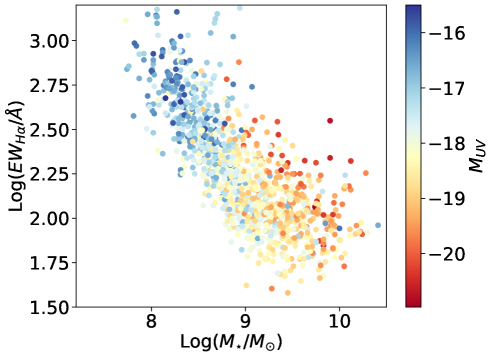
Figure 14: The rest-frame H$\alpha$ equivalent width as a function of the stellar mass. The color code translates the absolute UV magnitude of the sample.

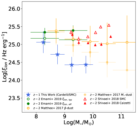
Figure 15: $\xi_{\mathrm{ion}}$as a function of the stellar mass. Our $\xi_{\mathrm{ion}}$ measurements are represented with filled blue stars. These $\xi_{\mathrm{ion}}$ estimates are derived by correcting H$\alpha$ line flux for nebular attenuation using the Cardelli curve and UV continuum luminosity for stellar extinction using SMC curve. Green filled (open) circles show the results of Emami et al. (2020) using the effective (standard) stacking method. The red filled (open) triangles show $\xi_{\mathrm{ion}}$ estimates by Shivaei et al. (2018) corrected for dust using Calzetti(SMC) curves. The results of Matthee et al. (2017) are shown with open, light-filled, and filled squares with dust corrections based on the $\beta$ slope, the mass-to-dust relation, and E(B-V) from SED fitting, respectively. More details on these literature results are given in Section 5.1

As we have seen, $\xi_{\mathrm{ion}}$ appears to correlate well with the H$\alpha$ equivalent width. At the same time, $EW_{\mathrm{H}\alpha}$ is anti-correlated with the stellar mass (cf. Figure 14). Similar results have been observed in galaxy samples at different redshifts (e.g. Reddy et al., 2018b; Faisst et al., 2019). It is therefore expected that $\xi_{\mathrm{ion}}$ will correlate with the stellar mass. However, several studies have found that $\xi_{\mathrm{ion}}$ is generally independent of the stellar mass. In particular, over the same mass range as our sample, Emami et al. (2020) find no evolution of $\xi_{\mathrm{ion}}$ between their two stacks binned in mass. At higher masses, Shivaei et al. (2018) find a small increase of 0.23 dex towards lower masses in the case of a Calzetti et al. (2000) attenuation curve for the stellar continuum emission. Figure 15 shows how $\xi_{\mathrm{ion}}$ is related to the stellar mass in our sample, together with literature results at higher redshifts. We see a higher $\xi_{\mathrm{ion}}$ at lower mass. Because of the redshift-evolution we have seen before, the general trend is slightly offset from the $z\sim 2$ results. The observed trend is unlikely the result of mass completeness (cf. Section 3). However, while the sample is generally limited by the equivalent width selection of EW$=80$ Å, it starts to be purely H$\alpha$-flux limited below $10^{9}$M_⊙(cf. Fig. 1). Such incompleteness could favor high $\xi_{\mathrm{ion}}$ values in lower-mass galaxies. Yet, we do not find high $\xi_{\mathrm{ion}}$ values in galaxies with stellar masses higher than $10^{9}$M_⊙, which is not affected by incompleteness. Deeper spectroscopic surveys of low-mass galaxies are required in order to confirm this trend.

The largest uncertainty remains the dust correction, as small variation in the dust content or the attenuation law has a large impact on the derived $\xi_{\mathrm{ion}}$, mainly because of the correction in the UV. We also over-plot the results of Matthee et al. (2017) with different dust correction methods, all of which show a trend of increase of $\xi_{\mathrm{ion}}$ towards lower masses, and highlight the dust-correction uncertainties. Note that, the $\beta$-based dust correction of Matthee et al. (2017) assumes $\beta_{0}=-2.21$ (Meurer et al., 1999), which contributes to the observed offset relative to our results.

We also investigate the relation between $\xi_{\mathrm{ion}}$ and the absolute UV magnitude, for which most studies do no report a clear correlation. As shown in Figure 16, Shivaei et al. (2018) and Emami et al. (2020) report no evolution with $M_{UV}$, while Matthee et al. (2017) show an increase towards fainter magnitudes. Similarly to our previous result regarding the stellar mass, faint galaxies show significantly higher ionizing efficiency. At even fainter magnitudes than our sample, a stacking analysis of a sample of LAEs at $z=4-5$ by Maseda et al. (2020) shows $\xi_{\mathrm{ion}}$ falling along this trend.

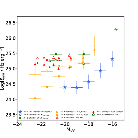
Figure 16: $\xi_{\mathrm{ion}}$ as a function of the absolute UV magnitude. Our $\xi_{\mathrm{ion}}$ estimates and literature results are represented with the same color code as in Figure 15. In addition, the results of Bouwens et al. (2016) at $3.8<z<5.0$ are represented with red circles. Their measurements are inferred from IRAC-based H$\alpha$ fluxes and corrected for dust attenuation using the $\beta$ slope and the SMC extinction curve. We also plot the result of Maseda et al. (2020) who similarly derived $\xi_{\mathrm{ion}}$ for a sample of Ly$\alpha$ emitters at $4<z<5$ using IRAC excess to estimate the H$\alpha$ flux. No dust correction was applied.

7 Implications for reionization

Early star-forming galaxies are currently the best candidates for driving cosmic reionization (Robertson et al., 2015; Bouwens et al., 2015; Atek et al., 2015). Given the most recent observational constraints on the shape of the UV luminosity function at $z>6$, low-mass galaxies could provide the bulk of the ionization budget (Livermore et al., 2017; Atek et al., 2018; Ishigaki et al., 2018; Finkelstein et al., 2019). However, precise knowledge of the ionizing properties of early galaxies and the escape fraction of ionizing radiation is still required to infer their exact contribution to reionization. Since such investigations are still challenging at $z>6$, many studies rely on lower-redshift galaxies, with the underlying assumption that they have the same properties as early galaxies. Therefore, it is important to focus on low-mass galaxies that are more representative of the galaxy population at the epoch of reionization.

It is clear that many physical properties and the SFH of low-mass galaxies are different from what is seen in their massive counterpart. The prevalence of intense emission lines, for instance, is much higher in low-mass galaxies, and increases with redshift. Star formation proceeds in successive bursts in low-mass galaxies, rather than a steady and constant star formation rate. Figure 8 shows how the relative increase in the recent SFR, as traced by H$\alpha$ relative to the averaged past SFR, as traced by the UV, indicate a recent burst of star formation in low-mass galaxies. While these observations cannot reveal successive SF bursts, many hydrodynamical simulations show that bursty star formation indeed happens mostly in low-mass galaxies, and can reproduce the observed variations of H$\alpha$/UV luminosity ratios. (Shen et al., 2014; Domínguez et al., 2015; Sparre et al., 2017; Emami et al., 2019). Confronting numerical simulations to the present observations is out of the scope of this paper and will be investigated in future work. Overall, understanding the burstiness parameters in these galaxies is crucial for several reasons:

• While the canonical value of Log($\xi_{\mathrm{ion}}$) $=25.2$, based on a constant star formation, might be adequate for massive galaxies, such assumptions do not hold in low-mass galaxies. Hydrodynamical simulations have shown that bursty star formation history leads to large variations in $\xi_{\mathrm{ion}}$ compared to constant SFH (e.g. Domínguez et al., 2015), which means the observed LyC photon production is not necessarily representative of the average value in these galaxies. For instance, these galaxies may remain undetected in LyC following a burst of star formation, although their average LyC production is high, and even if they have a high escape fraction. This is because it takes about 5 Myr for LyC emission to decrease by an order of magnitude after the burst, whereas the escape fraction will be significant only after 10 Myr, which corresponds to the supernovae timescale. However, accounting for binary stars in stellar population models (e.g. Stanway & Eldridge, 2018) lead to a significant increase in the number of ionizing photons produced over a larger range of masses, which result in a significant ionizing emission beyond 10 Myr (e.g. Chisholm et al., 2019).

• Bursty star formation also means that star formation feedback, which is responsible for disrupting the neutral ISM and clearing sight lines, will have significant impact on the LyC escape fraction. Hydrodynamical simulations also find large time variations of the escape fraction in low-mass galaxies, driven by supernovae explosions of massive stars (Kimm & Cen, 2014; Trebitsch et al., 2017). We note that in estimating $\xi_{\mathrm{ion}}$, we assumed $f_{esc}$$=0$. This is only a convention to ensure a fair comparison with literature results and the redshift-evolution of $\xi_{\mathrm{ion}}$. The most recent observing campaigns show a wide range of values for $f_{esc}$ at different redshifts (Izotov et al., 2016, 2018; Shapley et al., 2016; Vanzella et al., 2018; Flury et al., 2022). While empirically constraining the evolution of $f_{esc}$ remains challenging, hydrodynamical simulations find correlations with galaxy properties. For example, $f_{esc}$ increases with increasing star formation efficiency (or sSFR) and decreasing metallicity (e.g. Kimm et al., 2019).

These two quantities are pivotal in estimating the total ionizing power of galaxies. In addition to their dependency with galaxy physical parameters, these quantities might also be intertwined, as a higher ionizing photon production is likely followed by an increase in the escape fraction. Both their average values seem to increase with redshift, indicating a higher ionizing power in early galaxies than their low$-z$ analogs.

8 Conclusions

In this work, we used a combination of HST grism spectroscopy from the 3DHST survey and UV imaging from the HDUV survey for a large sample of 1167 galaxies across a redshift range of $0.7<z<1.5$. This represents a unique sample with its combination of direct measurements of H$\alpha$ down to an emission line flux limit of $1.5\times 10^{-17}$ erg s^-1 cm^-2 and deep UV imaging down to $M\sim 28$ mag. This combination enables us to probe star formation and UV output down to low stellar masses between $\sim 10^{8}$ and $10^{10}$ M_⊙. We have explored the star formation histories of these low-mass galaxies and estimated their ionizing efficiency $\xi_{\mathrm{ion}}$. In an attempt to extrapolate these findings to higher-redshift galaxies, we also explored how these parameters evolve with the physical properties of galaxies and with redshift.

We used the H$\alpha$ emission to infer the ionizing photon production rate, which in turn was combined with the UV luminosity at 1500 Å to compute the ionizing efficiency $\xi_{\mathrm{ion}}$. For removing the attenuation due to dust, we used the Cardelli curve to correct the H$\alpha$ flux and the SMC curve to correct the UV luminosity. With this combination, we obtained a median ionizing efficiency of Log($\xi_{\mathrm{ion}}$/erg^-1 Hz)$=24.80\pm 0.26$. While adopting different curves, the nebular attenuation has little impact on $\xi_{\mathrm{ion}}$  the UV attenuation is a source of significant uncertainty. For example, adopting Calzetti et al. (2000) law for the UV attenuation reduces the above median $\xi_{\mathrm{ion}}$ by 0.54 dex. Overall, our determination is significantly lower than literature results at higher redshifts. We find a clear evolution with lookback time, ranging from Log($\xi_{\mathrm{ion}}$)$=24.70$ at $t_{L}\sim 8.3$ Gyr to Log($\xi_{\mathrm{ion}}$)$=25.54$ at $t_{L}\sim 12.7$ Gyr. This evolution can be explained by higher star formation efficiency and higher emission line EWs on average at higher redshifts.

Investigating the relation between $\xi_{\mathrm{ion}}$ and galaxy properties:

• We observe a strong correlation with the H$\alpha$ equivalent width, consistent with the previous findings at different redshifts (Tang et al., 2019; Matthee et al., 2017; Reddy et al., 2018b; Emami et al., 2019).

• We found that $\xi_{\mathrm{ion}}$ is anti-correlated with stellar mass. This result should not be surprising since we also observe a strong anti-correlation between $EW_{\mathrm{H}\alpha}$ and stellar mass. However, incompleteness at the low-mass end likely affects the slope of the correlation. Previous studies found that $\xi_{\mathrm{ion}}$ is mostly independent of the stellar mass (Shivaei et al., 2018; Emami et al., 2019).

• Similarly, there is an evolution with absolute UV magnitude where fainter galaxies show higher $\xi_{\mathrm{ion}}$ values. Studies by Matthee et al. (2017) and Maseda et al. (2020) show results consistent with this trend.

When considering the SFR-M_⋆ relation, we find that a significant fraction of our sample lies above the main sequence, established at a similar redshift (Whitaker et al., 2014; Schreiber et al., 2015). Only galaxies around $EW_{\mathrm{H}\alpha}$ $\sim 100$ Å follow the MS, while higher $EW_{\mathrm{H}\alpha}$ galaxies depart from the MS, presumably because of an elevated instantaneous SFR following a recent burst. This is particularly true for lower-mass galaxies, below 10⁹ M_⊙, where high EWs are more common and contribute to a larger dispersion in the MS relation.

This result is confirmed when comparing the H$\alpha$ and UV continuum SFR indicators as a function of mass. We observe high SFR_Hα/SFR_UV ratios in galaxies with $10^{9}$ M_⊙. Unsurprisingly, these galaxies also show the highest $EW_{\mathrm{H}\alpha}$. Given the selection bias towards strong H$\alpha$ emitters in low-mass galaxies, these results can also be characterized as a higher scatter in the SFR_Hα/SFR_UV distribution in lower-mass galaxies, as it has been observed in previous studies (Weisz et al., 2012; Guo et al., 2016; Sparre et al., 2017; Emami et al., 2019). Faisst et al. (2019) results show that 50% of galaxies show a significant excess (more than a factor of 2) in SFR derived from H$\alpha$ with respect to the equilibrium. These galaxies also show the highest H$\alpha$ equivalent widths. In general, there is a large scatter around the equilibrium value of SFR_Hα/SFR_UV.

On the other hand, Broussard et al. (2019) compare theoretical predictions from semi-analytical models and hydrodynamical simulations to 3D-HST observations to infer the SF burstiness. They define the burstiness parameter $\eta$ as the logarithm of the ratio between SFR_Hα and SFR_UV. They find a positive correlation between the average of $\eta$ and stellar mass, and the scatter appears to be independent of the stellar mass. They note however that this correlation could be due to systematics in 3D-HST data that are not implemented in mock galaxies or to the dust prescriptions used. Our findings are in disagreement with those results, since we find that (i) the SFR_Hα/SFR_UV increases towards lower masses, even when using the same dust prescription to correct the H$\alpha$ and the UV emissions (Bottom-right panel of Figure 18); or (ii) given the selection effects (see Section 4.2) the scatter of SFR_Hα/SFR_UV ratio increases towards lower masses. This disagreement could be due to differences in both the sample selection and the methodology. Firstly, it is unclear whether the population of low-mass galaxies (fainter than H=24 AB mag) used in Broussard et al. (2019) has gone through additional checks including visual inspection, as it has been done in the present study. Indeed, this sub-sample of galaxies in the 3D-HST catalog is prone to uncertain measurements and spurious spectral identifications. Secondly, the SED fitting procedure and parameters used to derive their stellar population properties are different from the ones used in our study.

Some theoretical studies also show that burstiness is common in high-redshift galaxies across a wide mass range, whereas others show that only low-mass galaxies remain bursty all the way down to $z=0$ (Muratov et al., 2015; Flores Velázquez et al., 2020)). Our results suggest that burstiness parameters such as the duration of the burst or the duty cycle can differ from theoretical predictions. The prevalence of galaxies with enhanced H$\alpha$ relative to UV emission requires star formation variation on short time scales (less than 10 Myr) and/or short idle time between burst episodes on a rapid duty cycle. Direct implications on models of galaxy formation include modifications in the balance between the infall of gas, on one hand, and the ejection of gas or photoionization by the UV background, on the other hand.

Finally, a realistic model of reionization requires the convolution of the galaxy UV LF with physically-motivated ionization properties of galaxies. Recent attempts based on current observations lead to a variety of conclusions regarding the nature of galaxies contributing the most to reionization (e.g. Finkelstein et al., 2019; Naidu et al., 2020). A better understanding of the burstiness of galaxies and an accurate assessment of the volumetric escape fraction of galaxies (e.g. as a function of stellar mass) through deep LyC and rest-frame optical observations are needed to improve on this front.

Future NIR spectroscopic observations with the upcoming JWST will help obtain accurate measurements of the SFR and dust attenuation through the Balmer decrement for a large sample of galaxies across a wide range of redshifts to investigate in details the SF burstiness in galaxies down to even lower masses.

Data Availability

The data underlying this article are publicly available in the MAST archive at https://archive.stsci.edu/prepds/3d-hst/ and https://archive.stsci.edu/prepds/hduv/.

Appendix A Luminosity completeness

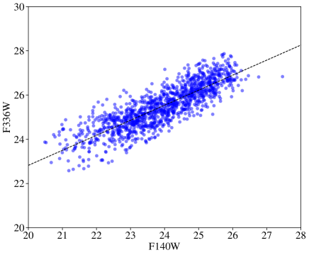
Figure 17: The UV magnitude in the F336W filter versus the NIR magnitude in the F140W filter for the $\xi_{\mathrm{ion}}$ sample. The dashed line shows the best-fit relation

In section 5, in order to estimate the completeness of our sample in terms of $\xi_{\mathrm{ion}}$ measurements, we combined the H$\alpha$ flux limit and the $EW_{\mathrm{H}\alpha}$. We simulated a sample of $EW_{\mathrm{H}\alpha}$ following the observed distribution, applying the same selection cut at 80Å. A combination with the H$\alpha$ flux limit gives a distribution in F140W magnitudes (rest-frame optical continuum). For the second term $L_{\rm UV}$, we use the observed correlation between the UV (F336W) and NIR (F140W) magnitudes and its associated dispersion. Figure 17 shows this relation, with a correlation of $UV_{mag}=(0.68\pm 0.012)\times H_{mag}+(9.22\pm 0.29)$

Appendix B Dust corrections

To explore how the choice of dust laws affects the burstiness results, we computed the SFR_Hα/SFR_UV ratio as a function of stellar mass for four different combinations of nebular/stellar corrections. The results are shown in Figure B. We first adopt the Calzetti attenuation law for both the SFR_Hα and SFR_UV (Top-left panel). As we have explained in Section 3.1 (see also Table 1), changing the dust law leads to significant difference in the correction factors mainly in the UV domain. Therefore, the adoption of the Calzetti law for the UV makes the SFR_UV significantly larger, especially for the more massive galaxies, which makes the SFR_Hα/SFR_UV much lower. The net result is a stronger dependence of the burstiness with stellar mass. We also investigate the following combinations: SMC/SMC and the Calzetti/Calzetti, but this time deriving the nebular attenuation from the stellar one, assuming a ratio of $E_{B-V,\mathrm{stars}}$/$E_{B-V,\mathrm{gas}}$=0.44. The fiducial combination Cardelli/SMC is also shown. These two combinations have little impact on the general trend of the SFR ratio, apart from slightly elevating the normalization of the bulk of the sample.

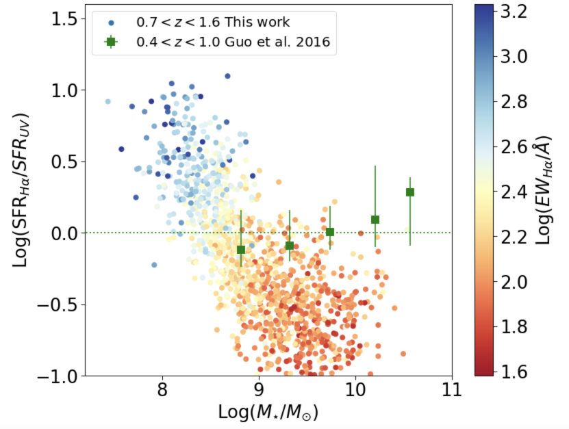
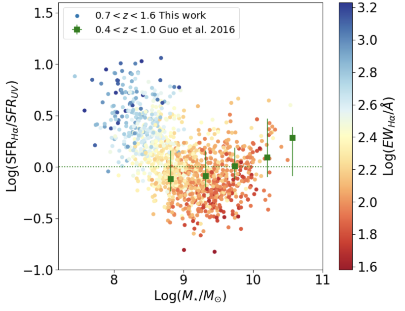
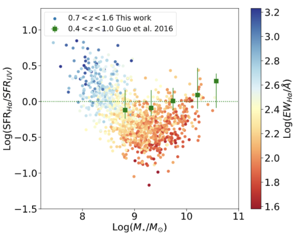
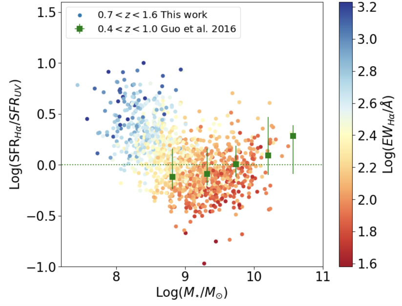
Figure 18: Effects of dust laws on the variations of the SFR_Hα/SFR_UV as a function of stellar mass. Four combinations for nebular/stellar dust are tested here. Top-left: Calzetti/Calzetti, top-right: SMC/SMC, Bottom-left: Cardelli/SMC, Bottom-right: Calzetti/Calzetti assuming $E_{B-V,\mathrm{stars}}$=0.44$E_{B-V,\mathrm{gas}}$. The color code is the same as in Figure 8.

Appendix C Intrinsic UV slope

In computing the dust extinction of the UV stellar continuum, we have measured and compared the observed UV slope $\beta$ with the intrinsic slope $\beta_{0}$. We adopted a value of $\beta_{0}=-2.62$ derived by Reddy et al. (2018a). This value is derived for a sample of $z\sim 2$ galaxies, assuming a stellar population model with an age of 100 Myr, $Z=0.14Z_{\odot}$ metallicity and a constant star formation history. To investigate the importance of this parameter choice, we also used the canonical value of $\beta_{0}=-2.23$ (Meurer et al., 1999) for comparison, which assumes a constant star formation history and a solar metallicity. In (Figure 19), we show the effect on the SFR_Hα/SFR_UV ratio as a function of stellar mass. We observe a slight elevation of the global values, with no noticeable impact on the overall trend. In Meurer et al. (1999), it is also shown that variations of the stellar populations properties, including instantaneous bursts of star formation, IMF and metallicity lead to variations between $\beta_{0}=-2.0$ and $\beta_{0}=-2.6$.

Similarly, we also show in Figure 20 the impact of adopting a different intrinsic UV slope on the $\xi_{\mathrm{ion}}$ distribution. First, adopting $\beta_{int}=-2.23$ results in a median value of Log($\xi_{\mathrm{ion}}$/erg^-1 Hz)$=25.12\pm 0.26$, adopting the fiducial dust correction combination Cardelli/SMC. For reference, we found Log($\xi_{\mathrm{ion}}$/erg^-1 Hz)$=24.80\pm 0.26$ when using $\beta_{int}=-2.62$. We also included a dispersion in the intrinsic UV slope by uniformly sampling the range $-2.62<\beta<-2.23$, resulting in the right panel of Figure 20. We find a median value of Log($\xi_{\mathrm{ion}}$/erg^-1 Hz)$=24.89\pm 0.27$. A slight increase of 0.05 dex in the dispersion of the $\xi_{\mathrm{ion}}$ distribution is notably observed for the Cardelli/Calzetti durst correction.

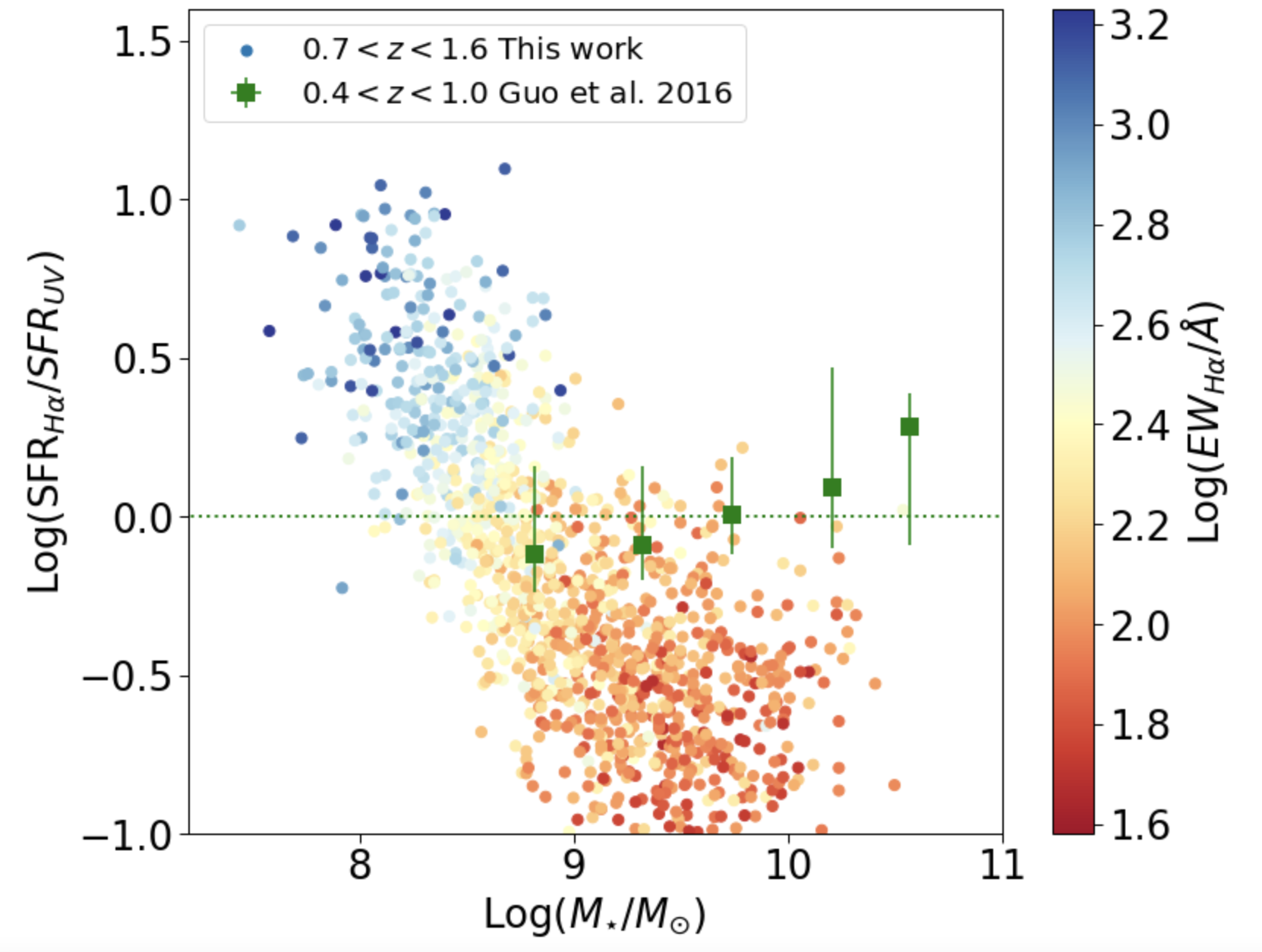
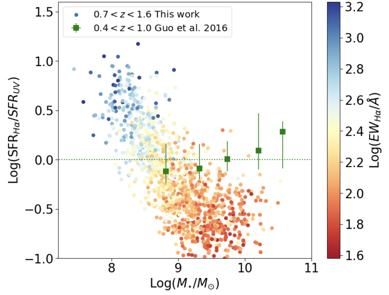
Figure 19: The impact of the intrinsic UV slope $\beta_{int}$ on the correlation between the SFR_Hα/SFR_UV and the stellar mass. We compare, in the left panel, the value adopted in this study $\beta_{0}=-2.62$ (Reddy et al., 2018a) and, in the right panel, the canonical value of $\beta_{0}=-2.21$ (Meurer et al., 1999). We used the Calzetti et al. (2000) attenuation curve for both the stellar and nebular dust correction (cf. fig. 18).

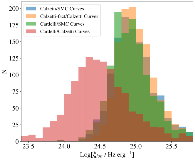
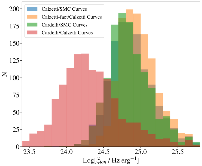
Figure 20: The impact of the intrinsic UV slope $\beta_{int}$ on $\xi_{\mathrm{ion}}$ distribution. The left panel shows the same distributions shown in figure 10 but adopting $\beta_{int}=-2.23$ (Meurer et al., 1999) instead of $\beta_{int}=-2.62$ (Reddy et al., 2018a). The right panel shows the result of using a dispersion in $\beta_{int}$ in the range defined by these two values.

References

- Atek et al. (2010) Atek H., et al., 2010, ApJ, 723, 104
- Atek et al. (2011) Atek H., et al., 2011, ApJ, 743, 121
- Atek et al. (2014) Atek H., et al., 2014, ApJ, 789, 96
- Atek et al. (2015) Atek H., et al., 2015, ApJ, 814, 69
- Atek et al. (2018) Atek H., Richard J., Kneib J.-P., Schaerer D., 2018, MNRAS, 479, 5184
- Bian et al. (2017) Bian F., Fan X., McGreer I., Cai Z., Jiang L., 2017, ApJ, 837, L12
- Boogaard et al. (2018) Boogaard L. A., et al., 2018, A&A, 619, A27
- Bouwens et al. (2015) Bouwens R. J., Illingworth G. D., Oesch P. A., Caruana J., Holwerda B., Smit R., Wilkins S., 2015, ApJ, 811, 140
- Bouwens et al. (2016) Bouwens R. J., Smit R., Labbé I., Franx M., Caruana J., Oesch P., Stefanon M., Rasappu N., 2016, ApJ, 831, 176
- Brammer et al. (2012) Brammer G. B., et al., 2012, ApJS, 200, 13
- Brinchmann et al. (2004) Brinchmann J., Charlot S., White S. D. M., Tremonti C., Kauffmann G., Heckman T., Brinkmann J., 2004, MNRAS, 351, 1151
- Broussard et al. (2019) Broussard A., et al., 2019, ApJ, 873, 74
- Calzetti (2013) Calzetti D., 2013, Star Formation Rate Indicators. p. 419
- Calzetti et al. (2000) Calzetti D., Armus L., Bohlin R. C., Kinney A. L., Koornneef J., Storchi-Bergmann T., 2000, ApJ, 533, 682
- Cardelli et al. (1989) Cardelli J. A., Clayton G. C., Mathis J. S., 1989, ApJ, 345, 245
- Castellano et al. (2014) Castellano M., et al., 2014, A&A, 566, A19
- Chabrier (2003) Chabrier G., 2003, ApJ, 586, L133
- Chan et al. (2015) Chan T. K., Kereš D., Oñorbe J., Hopkins P. F., Muratov A. L., Faucher-Giguère C. A., Quataert E., 2015, MNRAS, 454, 2981
- Chary & Elbaz (2001) Chary R., Elbaz D., 2001, ApJ, 556, 562
- Chisholm et al. (2019) Chisholm J., Rigby J. R., Bayliss M., Berg D. A., Dahle H., Gladders M., Sharon K., 2019, ApJ, 882, 182
- Cowie et al. (2016) Cowie L. L., Barger A. J., Songaila A., 2016, ApJ, 817, 57
- Domínguez et al. (2013) Domínguez A., et al., 2013, ApJ, 763, 145
- Domínguez et al. (2015) Domínguez A., Siana B., Brooks A. M., Christensen C. R., Bruzual G., Stark D. P., Alavi A., 2015, MNRAS, 451, 839
- Elbaz et al. (2007) Elbaz D., et al., 2007, A&A, 468, 33
- Emami et al. (2019) Emami N., Siana B., Weisz D. R., Johnson B. D., Ma X., El-Badry K., 2019, ApJ, 881, 71
- Emami et al. (2020) Emami N., Siana B., Alavi A., Gburek T., Freeman W. R., Richard J., Weisz D. R., Stark D. P., 2020, ApJ, 895, 116
- Faisst et al. (2016) Faisst A. L., et al., 2016, ApJ, 821, 122
- Faisst et al. (2019) Faisst A. L., Capak P. L., Emami N., Tacchella S., Larson K. L., 2019, ApJ, 884, 133
- Faucher-Giguère (2018) Faucher-Giguère C.-A., 2018, MNRAS, 473, 3717
- Finkelstein et al. (2019) Finkelstein S. L., et al., 2019, ApJ, 879, 36
- Flores Velázquez et al. (2020) Flores Velázquez J. A., et al., 2020, arXiv e-prints, p. arXiv:2008.08582
- Flury et al. (2022) Flury S. R., et al., 2022, arXiv e-prints, p. arXiv:2201.11716
- Foreman-Mackey et al. (2013) Foreman-Mackey D., Hogg D. W., Lang D., Goodman J., 2013, PASP, 125, 306
- Fumagalli et al. (2011) Fumagalli M., da Silva R. L., Krumholz M. R., 2011, ApJ, 741, L26
- Garn & Best (2010) Garn T., Best P. N., 2010, MNRAS, 409, 421
- Gordon et al. (2003) Gordon K. D., Clayton G. C., Misselt K. A., Land olt A. U., Wolff M. J., 2003, ApJ, 594, 279
- Grogin et al. (2011) Grogin N. A., et al., 2011, ApJS, 197, 35
- Guo et al. (2016) Guo Y., et al., 2016, ApJ, 833, 37
- Hao et al. (2011) Hao C.-N., Kennicutt R. C., Johnson B. D., Calzetti D., Dale D. A., Moustakas J., 2011, ApJ, 741, 124
- Ishigaki et al. (2018) Ishigaki M., Kawamata R., Ouchi M., Oguri M., Shimasaku K., Ono Y., 2018, ApJ, 854, 73
- Izotov et al. (2016) Izotov Y. I., Orlitová I., Schaerer D., Thuan T. X., Verhamme A., Guseva N. G., Worseck G., 2016, Nature, 529, 178
- Izotov et al. (2018) Izotov Y. I., Worseck G., Schaerer D., Guseva N. G., Thuan T. X., Fricke Verhamme A., Orlitová I., 2018, MNRAS, 478, 4851
- Kennicutt & Evans (2012) Kennicutt R. C., Evans N. J., 2012, ARA&A, 50, 531
- Kimm & Cen (2014) Kimm T., Cen R., 2014, ApJ, 788, 121
- Kimm et al. (2019) Kimm T., Blaizot J., Garel T., Michel-Dansac L., Katz H., Rosdahl J., Verhamme A., Haehnelt M., 2019, MNRAS, 486, 2215
- Kriek et al. (2015) Kriek M., et al., 2015, ApJS, 218, 15
- Kurczynski et al. (2016) Kurczynski P., et al., 2016, ApJ, 820, L1
- Lam et al. (2019) Lam D., et al., 2019, A&A, 627, A164
- Leitherer & Heckman (1995) Leitherer C., Heckman T. M., 1995, ApJS, 96, 9
- Leitherer et al. (1999) Leitherer C., et al., 1999, ApJS, 123, 3
- Livermore et al. (2017) Livermore R. C., Finkelstein S. L., Lotz J. M., 2017, ApJ, 835, 113
- Maseda et al. (2020) Maseda M. V., et al., 2020, MNRAS, 493, 5120
- Matthee et al. (2017) Matthee J., Sobral D., Best P., Khostovan A. A., Oteo I., Bouwens R., Röttgering H., 2017, MNRAS, 465, 3637
- Meurer et al. (1999) Meurer G. R., Heckman T. M., Calzetti D., 1999, ApJ, 521, 64
- Meurer et al. (2009) Meurer G. R., et al., 2009, ApJ, 695, 765
- Momcheva et al. (2016) Momcheva I. G., et al., 2016, ApJS, 225, 27
- Muratov et al. (2015) Muratov A. L., Kereš D., Faucher-Giguère C.-A., Hopkins P. F., Quataert E., Murray N., 2015, MNRAS, 454, 2691
- Naidu et al. (2020) Naidu R. P., Tacchella S., Mason C. A., Bose S., Oesch P. A., Conroy C., 2020, ApJ, 892, 109
- Nakajima et al. (2016) Nakajima K., Ellis R. S., Iwata I., Inoue A. K., Kusakabe H., Ouchi M., Robertson B. E., 2016, ApJ, 831, L9
- Noeske et al. (2007) Noeske K. G., et al., 2007, ApJ, 660, L43
- Oesch et al. (2018) Oesch P. A., et al., 2018, ApJS, 237, 12
- Oke & Gunn (1983) Oke J. B., Gunn J. E., 1983, ApJ, 266, 713
- Osterbrock (1989) Osterbrock D. E., 1989, Astrophysics of gaseous nebulae and active galactic nuclei. Research supported by the University of California, John Simon Guggenheim Memorial Foundation, University of Minnesota, et al. Mill Valley, CA, University Science Books, 1989, 422 p.
- Pelliccia et al. (2020) Pelliccia D., et al., 2020, ApJ, 896, L26
- Pflamm-Altenburg et al. (2009) Pflamm-Altenburg J., Weidner C., Kroupa P., 2009, MNRAS, 395, 394
- Price et al. (2014) Price S. H., et al., 2014, ApJ, 788, 86
- Read et al. (2016) Read J. I., Agertz O., Collins M. L. M., 2016, MNRAS, 459, 2573
- Reddy et al. (2015) Reddy N. A., et al., 2015, ApJ, 806, 259
- Reddy et al. (2018a) Reddy N. A., et al., 2018a, ApJ, 853, 56
- Reddy et al. (2018b) Reddy N. A., et al., 2018b, ApJ, 869, 92
- Rivera-Thorsen et al. (2019) Rivera-Thorsen T. E., et al., 2019, Science, 366, 738
- Robertson et al. (2013) Robertson B. E., et al., 2013, ApJ, 768, 71
- Robertson et al. (2015) Robertson B. E., Ellis R. S., Furlanetto S. R., Dunlop J. S., 2015, ApJ, 802, L19
- Rodighiero et al. (2011) Rodighiero G., et al., 2011, ApJ, 739, L40
- Rutkowski et al. (2017) Rutkowski M. J., et al., 2017, ApJ, 841, L27
- Salim & Narayanan (2020) Salim S., Narayanan D., 2020, ARA&A, 58, 529
- Schreiber et al. (2015) Schreiber C., et al., 2015, A&A, 575, A74
- Shapley et al. (2016) Shapley A. E., Steidel C. C., Strom A. L., Bogosavljević M., Reddy N. A., Siana B., Mostardi R. E., Rudie G. C., 2016, ApJ, 826, L24
- Shen et al. (2014) Shen S., Madau P., Conroy C., Governato F., Mayer L., 2014, ApJ, 792, 99
- Shim et al. (2011) Shim H., Chary R.-R., Dickinson M., Lin L., Spinrad H., Stern D., Yan C.-H., 2011, ApJ, 738, 69
- Shivaei et al. (2018) Shivaei I., et al., 2018, ApJ, 855, 42
- Skelton et al. (2014) Skelton R. E., et al., 2014, ApJS, 214, 24
- Smit et al. (2014) Smit R., et al., 2014, ApJ, 784, 58
- Smit et al. (2016) Smit R., Bouwens R. J., Labbé I., Franx M., Wilkins S. M., Oesch P. A., 2016, ApJ, 833, 254
- Sobral et al. (2012) Sobral D., Best P. N., Matsuda Y., Smail I., Geach J. E., Cirasuolo M., 2012, MNRAS, 420, 1926
- Sparre et al. (2017) Sparre M., Hayward C. C., Feldmann R., Faucher-Giguère C.-A., Muratov A. L., Kereš D., Hopkins P. F., 2017, MNRAS, 466, 88
- Stanway & Eldridge (2018) Stanway E. R., Eldridge J. J., 2018, MNRAS, 479, 75
- Stark et al. (2015) Stark D. P., et al., 2015, MNRAS, 454, 1393
- Tang et al. (2019) Tang M., Stark D. P., Chevallard J., Charlot S., 2019, MNRAS, 489, 2572
- Teplitz et al. (2013) Teplitz H. I., et al., 2013, AJ, 146, 159
- Trebitsch et al. (2017) Trebitsch M., Blaizot J., Rosdahl J., Devriendt J., Slyz A., 2017, MNRAS, 470, 224
- Vanzella et al. (2016) Vanzella E., et al., 2016, ApJ, 825, 41
- Vanzella et al. (2018) Vanzella E., et al., 2018, MNRAS, 476, L15
- Weisz et al. (2012) Weisz D. R., et al., 2012, ApJ, 744, 44
- Whitaker et al. (2014) Whitaker K. E., et al., 2014, ApJ, 795, 104
- Wilkins et al. (2019) Wilkins S. M., Lovell C. C., Stanway E. R., 2019, MNRAS, 490, 5359
- Wisnioski et al. (2015) Wisnioski E., et al., 2015, ApJ, 799, 209
- Wuyts et al. (2011a) Wuyts S., et al., 2011a, ApJ, 738, 106
- Wuyts et al. (2011b) Wuyts S., et al., 2011b, ApJ, 742, 96
- de Barros et al. (2014) de Barros S., Schaerer D., Stark D. P., 2014, A&A, 563, A81