Improved estimator for numerical renormalization group calculations of the self-energy

Abstract

We present a new estimator for the self-energy based on a combination of two equations of motion and discuss its benefits for numerical renormalization group (NRG) calculations. In challenging regimes, NRG results from the standard estimator, a ratio of two correlators, often suffer from artifacts: The imaginary part of the retarded self-energy is not properly normalized and, at low energies, overshoots to unphysical values and displays wiggles. We show that the new estimator resolves the artifacts in these properties as they can be determined directly from the imaginary parts of auxiliary correlators and do not involve real parts obtained by Kramers–Kronig transform. Furthermore, we find that the new estimator yields converged results with reduced numerical effort (for a lower number of kept states) and thus is highly valuable when applying NRG to multiorbital systems. Our analysis is targeted at NRG treatments of quantum impurity models, especially those arising within dynamical mean-field theory, but most results can be straightforwardly generalized to other impurity or cluster solvers.

I Introduction

Quantum impurity systems, a small number of interacting degrees of freedom embedded in a noninteracting bath, play an important role in many-body physics. On the one hand, they are fascinating on their own right, serving as a paradigm for strong-coupling phenomena and as the underlying model of quantum dot devices Hanson et al. (2007). On the other hand, they gained much attention recently in the study of strongly correlated lattice systems within the dynamical mean-field theory (DMFT) Georges et al. (1996).

For conventional quantum impurity models, central dynamic correlation functions are, e.g., the spectral function (local density of states) or the magnetic susceptibility. By contrast, in DMFT, the quintessential object is the (local but frequency-dependent) self-energy. It enters many observables, such as the momentum-dependent spectral function (used to describe angle-resolved photoemission spectroscopy), all types of conductivities in transport measurements, nonlocal susceptibilities that make up structure factors, and is needed to determine the Fermi-liquid parameters that pervade most low-energy properties. Moreover, for almost all lattices—the popular Bethe lattice being an exception—the self-energy is the crucial ingredient of the DMFT self-consistency iteration Georges et al. (1996).

The numerical renormalization group (NRG) Wilson (1975) is the gold standard for solving quantum impurity models Bulla et al. (2008). It is often used as a real-frequency impurity solver for DMFT, in Hubbard models with one Bulla (1999); Bulla et al. (2001); Deng et al. (2013); Lee et al. (2017); Vučičević et al. (2019); Vranić et al. (2020); Vučičević and Žitko (2021a); *Vucicevic2021b, two Pruschke and Bulla (2005); Peters and Pruschke (2010a); *Peters2010b; Peters et al. (2011); Greger et al. (2013, ); Kugler and Kotliar , and three orbitals Stadler et al. (2016, 2019); Kugler et al. (2019); Stadler et al. (2021), and recently even for realistic material systems Kugler et al. (2020). Modern formulations of NRG, a.k.a. full density-matrix (fdm) NRG Peters et al. (2006); Weichselbaum and von Delft (2007), give very accurate results for correlation functions of local operators. Yet, the self-energy $\Sigma$ is no such correlation function but an irreducible vertex object, and must be computed by different means. Since a direct inversion of the Dyson equation is numerically disadvantageous, $\Sigma$ is routinely computed through an equation of motion (eom) as a quotient between two correlators Bulla et al. (1998). In challenging (e.g., multiorbital) situations, however, the results for $\Sigma$ are not always as accurate as one expects from NRG. First, its spectral weight is not guaranteed to be properly normalized in fdm NRG, so that the (analytically known) high-frequency asymptote may be violated. Moreover, the imaginary part of the retarded self-energy, $\mathrm{Im}\!\;\Sigma_{\nu}$, can overshoot to positive values at low energies even though causality requires $\mathrm{Im}\!\;\Sigma_{\nu}\!\leq\!0$. This is often accompanied by wiggles in small values of $\mathrm{Im}\!\;\Sigma_{\nu}$.

In fact, while the high-energy resolution of NRG can be increased by averaging techniques Žitko and Pruschke (2009); Lee and Weichselbaum (2016); Lee et al. (2017), these tricks do not help much in resolving the problems of $\mathrm{Im}\!\;\Sigma_{\nu}$ at low energies—where NRG is most powerful. So far, the overshooting and wiggles in $\mathrm{Im}\!\;\Sigma_{\nu}$ could only be tackled by brute-force increase of numerical effort (increasing the number of kept states), so that accurate results for $\Sigma$ were a computational bottleneck.

In this paper, we present a new formula for the self-energy, based on a combination of a one- Bulla et al. (1998) and twofold Kaufmann et al. (2019) application of the eom. This result strongly alleviates the previously mentioned artifacts: The high-frequency asymptote of $\mathrm{Re}\!\;\Sigma$ is fulfilled exactly, overshooting of $\mathrm{Im}\!\;\Sigma$ is ruled out, and the value of $\mathrm{Im}\!\;\Sigma$ at zero energy is improved by several orders of magnitude. Our formula involves three instead of two Bulla et al. (1998) correlators. While this naively increases the numerical costs by a factor of $1.5$, we find that accurate results with the new formula are obtained already with less numerical effort (a lower number of kept states) compared to the standard scheme. Hence, our approach also makes NRG computations of $\Sigma$ more efficient and thus helps to equip DMFT+NRG with the tools needed for treating Hubbard models with ever more orbitals.

The rest of the paper is organized as follows. In Sec. II, we give an overview of the theoretical framework as well as the previous and new self-energy estimators. The derivation of these expressions and their properties is found in the subsequent Sec. III. In Sec. IV, we demonstrate the benefits of the new approach with numerical results. There, we start with the single-orbital Anderson impurity model and proceed with one-, two-, and three-orbital Hubbard models treated in DMFT. Section V contains our conclusions, Appendix A discusses the generalization to matrix-valued correlation functions, and Appendix B provides additional numerical data.

II Overview

II.1 Definitions

Quantum impurity models are naturally divided into the interacting impurity and the noninteracting bath. We denote electron creation operators of the former by $d^{\dagger}_{\alpha}$ and those of the latter by $c^{\dagger}_{k\alpha}$. The index $\alpha$ enumerates spin ($\sigma$) and possibly orbital ($m$) quantum numbers; the bath modes are further labeled by $k$, standing, e.g., for momentum. The noninteracting part of the Hamiltonian $H\!=\!H_{0}+H_{\mathrm{int}}$ generally reads

$$H_{0} =\textstyle\sum_{\alpha}\epsilon_{d,\alpha}d^{\dagger}_{\alpha}d_{\alpha}+\sum_{k,\alpha}\epsilon_{k\alpha}c^{\dagger}_{k\alpha}c_{k\alpha}$$

$$\ \textstyle+\sum_{k,\alpha}(V_{k\alpha}d_{\alpha}^{\dagger}c_{k\alpha}+\mathrm{H.c.}).$$ (1)

For the interacting part, we consider two examples. The single-orbital ($\alpha\!=\!\sigma$) Anderson impurity model Anderson (1961) has

$$H_{\mathrm{int}}=Un_{\uparrow}n_{\downarrow},\quad n_{\sigma}=d^{\dagger}_{\sigma}d_{\sigma}.$$ (2)

In the multiorbital case [$\alpha=(\sigma,m)$], we use the generalization of Eq. (2) introduced by Dworin and Narath Dworin and Narath (1970); Georges et al. (2013),

$$H_{\mathrm{int}}=\tfrac{3}{4}JN+\tfrac{1}{2}(U-\tfrac{3}{2}J)N(N-1)-J{\bm{S}}^{2},$$ (3)

where $N=\sum_{\alpha}d^{\dagger}_{\alpha}d_{\alpha}$ and ${\bm{S}}=\sum_{\sigma\sigma^{\prime}m}d^{\dagger}_{\sigma^{\prime}m}{\bm{\tau}}_{\sigma^{\prime}\sigma}d_{\sigma m}$ with the Pauli matrices ${\bm{\tau}}$.

We will be interested in correlation functions involving the fundamental operators $d_{\alpha}$, $d_{\alpha}^{\dagger}$ as well as the auxiliary operators

$$q_{\alpha}=[d_{\alpha},H_{\mathrm{int}}],\quad q_{\alpha}^{\dagger}=[H_{\mathrm{int}},d_{\alpha}^{\dagger}].$$ (4)

They allow us to define four fermionic correlation functions:

$$\qquad G_{\alpha z} =\langle\mspace{-3.0mu}\langle d_{\alpha},d_{\alpha}^{\dagger}\rangle\mspace{-3.0mu}\rangle_{z}, \quad I_{\alpha z} =\langle\mspace{-3.0mu}\langle q_{\alpha},q_{\alpha}^{\dagger}\rangle\mspace{-3.0mu}\rangle_{z},$$ (5a)

$$\qquad F^{\mathrm{L}}_{\alpha z} =\langle\mspace{-3.0mu}\langle q_{\alpha},d_{\alpha}^{\dagger}\rangle\mspace{-3.0mu}\rangle_{z}, \quad F^{\mathrm{R}}_{\alpha z} =\langle\mspace{-3.0mu}\langle d_{\alpha},q_{\alpha}^{\dagger}\rangle\mspace{-3.0mu}\rangle_{z}.$$ (5b)

Here, our notation follows Ref. Bulla et al. (1998): $z$ is a complex frequency variable. It can be a discrete imaginary frequency, $\mathrm{i}\nu$, or a continuous real frequency $\nu$. In the former case, $\langle\mspace{-3.0mu}\langle A,B\rangle\mspace{-3.0mu}\rangle_{z}$ is the Fourier transform of the imaginary-time correlator $-\langle\mathit{T}A(\tau)B\rangle$, with the time-ordering operator $\mathit{T}$. In the latter, it corresponds to the retarded correlator $-\mathrm{i}\theta(t)\langle\{A(t),B\}\rangle$, with the step function $\theta$ and the anticommutator $\{\cdot,\cdot\}$.

In systems defined by Eqs. (1)–(3), the fermionic correlation functions are diagonal in $\alpha$ (and thus carry only a single subscript). It then follows (as shown below) that $F^{\mathrm{L}}_{\alpha z}=F^{\mathrm{R}}_{\alpha z}$; we will hence mostly drop the superscript. Appendix A addresses the case where $H_{0}$ has off-diagonal contributions and the correlation functions become matrix-valued. Then, $F^{\mathrm{L}}$ and $F^{\mathrm{R}}$ are not equal, but still related by symmetry. For a close connection of both situations, we often use matrix-type notation in the main text, too, and restore the superscripts $\mathrm{L}$, $\mathrm{R}$ in key places. Moreover, even for $\alpha$-diagonal computations, $F^{\mathrm{L}}_{\alpha z}=F^{\mathrm{R}}_{\alpha z}$ might be slightly violated numerically. It may then be helpful to use the matrix-type formulas, which are symmetric in $F^{\mathrm{L}}$ and $F^{\mathrm{R}}$.

Before moving on to the self-energy, let us briefly recall how correlators like $G_{\alpha z}$, $F_{\alpha z}$, and $I_{\alpha z}$ are obtained in NRG.

II.2 NRG correlation functions

In NRG, a general correlator $C_{\alpha z}$ is first computed as a discrete version of the spectral part $-\tfrac{1}{\pi}\mathrm{Im}\!\;C_{\alpha\nu}$. After broadening $\mathrm{Im}\!\;C_{\alpha\nu}$, the real part follows by Kramers–Kronig transform as

$$\mathrm{Re}\!\;C_{\alpha\nu}=-\frac{1}{\pi}\,\mathcal{P}\!\!\int\!\mathrm{d}\nu^{\prime}\,\frac{\mathrm{Im}\!\;C_{\alpha\nu^{\prime}}}{\nu-\nu^{\prime}}.$$ (6)

By construction of fdm NRG, the total weight of $\mathrm{Im}\!\;C_{\alpha\nu}$ is guaranteed to be exact Peters et al. (2006); Weichselbaum and von Delft (2007). Further, by the very nature of NRG, results for $\mathrm{Im}\!\;C_{\alpha\nu}$ are most accurate at low energies. Going to larger frequencies, $\mathrm{Im}\!\;C_{\alpha\nu}$ can be significantly less accurate, reflecting the logarithmic discretization of the hybridization function. Refined averaging and adaptive broadening techniques Žitko and Pruschke (2009); Lee and Weichselbaum (2016); Lee et al. (2017) help to minimize overbroadening. Yet, the approximate nature of $\mathrm{Im}\!\;C_{\alpha\nu}$ for large $\nu$ remains. In particular, it is known that the moments $C^{(n)}=-\tfrac{1}{\pi}\!\int\!\mathrm{d}\nu\,\nu^{n}\mathrm{Im}\!\;C_{\alpha\nu}$ are not reproduced exactly for $n>0$. Now, by Eq. (6), the large-energy inaccuracies of $\mathrm{Im}\!\;C_{\alpha\nu}$ are not only passed down to $\mathrm{Re}\!\;C_{\alpha\nu}$ but are also spread in frequency space. Hence, in the following, we will aim to minimize the effect of real parts of correlation functions in the computation of $\Sigma$.

II.3 Self-energy formulas

The self-energy is defined by the Dyson equation as

$$\Sigma_{\alpha z}=(G^{0}_{\alpha z})^{-1}-(G_{\alpha z})^{-1}.$$ (7)

Here, $G^{0}_{\alpha z}$ is the bare propagator, which can be written in terms of the hybridization function $\Delta_{\alpha z}$ as

$$(G^{0}_{\alpha z})^{-1} =z-\epsilon_{d,\alpha}-\Delta_{\alpha z},\qquad\Delta_{\alpha z}=\sum_{k}\frac{|V_{k\alpha}|^{2}}{z-\epsilon_{k\alpha}}.$$ (8)

The retarded self-energy fulfills the Kramers–Kronig relation

$$\mathrm{Re}\!\;\Sigma_{\alpha\nu}=\Sigma^{\mathrm{H}}_{\alpha}-\frac{1}{\pi}\,\mathcal{P}\!\!\int\!\mathrm{d}\nu^{\prime}\,\frac{\mathrm{Im}\!\;\Sigma_{\alpha\nu^{\prime}}}{\nu-\nu^{\prime}},$$ (9)

where $\Sigma^{\mathrm{H}}_{\alpha}$ is the constant Hartree part. This relates the high-frequency asymptote of the real part to the total weight in the imaginary part. We define the $1/\nu$ coefficient of $\mathrm{Re}\!\;\Sigma_{\alpha\nu}$ (or the $1/z$ coefficient of $\Sigma_{\alpha z}$) as the moment $\Sigma_{\alpha}^{(0)}$ which fulfills

$$\Sigma_{\alpha}^{(0)}=\lim_{|\nu|\to\infty}\nu\,(\mathrm{Re}\!\;\Sigma_{\alpha\nu}-\Sigma^{\mathrm{H}}_{\alpha})=-\frac{1}{\pi}\!\int\!\mathrm{d}\nu\,\mathrm{Im}\!\;\Sigma_{\alpha\nu}.$$ (10)

For many algorithms that yield $G_{\alpha z}$ directly, Eq. (7) is not ideal to extract $\Sigma$. In NRG, it is basically inapplicable since $G^{0}_{\alpha z}$ involves the exact, continuous hybridization function. By contrast, $G_{\alpha z}$ is the result of an approximate calculation where $\Delta_{\alpha z}$ was discretized. Thus, cancellations between $G^{0}_{\alpha z}$ and $G_{\alpha z}$ required for Eq. (7) do not work properly and induce large numerical errors. For this reason, NRG self-energies are routinely computed by means of an eom yielding Bulla et al. (1998)

$$\Sigma_{\alpha z}^{\mathrm{FG}}=F_{\alpha z}(G_{\alpha z})^{-1}.$$ (11)

Our new formula, based on a combination of a one- and twofold Kaufmann et al. (2019) application of the eom, reads

$$\Sigma_{\alpha z}^{\mathrm{IFG}}=\Sigma^{\mathrm{H}}_{\alpha}+I_{\alpha z}-F^{\mathrm{L}}_{\alpha z}(G_{\alpha z})^{-1}F^{\mathrm{R}}_{\alpha z}.$$ (12)

We restored the superscript on $F$ in light of matrix-valued applications (see Appendix A). In the given $\alpha$-diagonal setting, the last term can be simply written as $F_{\alpha z}^{2}/G_{\alpha z}$. Now, what are the advantages of Eq. (12) over Eq. (11)?

Focusing on the imaginary part, from Eq. (11), we get

$$\mathrm{Im}\!\;\Sigma^{\mathrm{FG}}_{\alpha\nu} =\frac{\mathrm{Im}\!\;F_{\alpha\nu}\mathrm{Re}\!\;G_{\alpha\nu}-\mathrm{Re}\!\;F_{\alpha\nu}\mathrm{Im}\!\;G_{\alpha\nu}}{|G_{\alpha\nu}|^{2}}.$$ (13)

Evidently, $\mathrm{Im}\!\;\Sigma^{\mathrm{FG}}_{\alpha\nu}$ is determined by the imaginary parts and the real parts of NRG correlators. One finds that the total weight $\!\int\!\mathrm{d}\nu\,\mathrm{Im}\!\;\Sigma^{\mathrm{FG}}_{\alpha\nu}$ typically does not give the exact value. Further, due to the real parts involved, $\mathrm{Im}\!\;\Sigma^{\mathrm{FG}}_{\alpha\nu}$ at low energies is less accurate than one is used to for imaginary parts of correlators computed directly with NRG. In challenging regimes, one encounters the aforementioned artifacts that $\mathrm{Im}\!\;\Sigma^{\mathrm{FG}}_{\alpha\nu}$ overshoots to positive values and displays wiggles for low $\nu$.

By contrast, for $\Sigma_{\alpha z}^{\mathrm{IFG}}$, we will show that both the total weight of $\mathrm{Im}\!\;\Sigma^{\mathrm{IFG}}_{\alpha\nu}$, as an important high-energy property, as well as the low-energy behavior of $\mathrm{Im}\!\;\Sigma^{\mathrm{IFG}}_{\alpha\nu}$ is determined by the imaginary parts of NRG correlators only. Indeed, we have

$$\!\int\!\mathrm{d}\nu\,\mathrm{Im}\!\;\Sigma_{\alpha\nu}^{\mathrm{IFG}} =\!\int\!\mathrm{d}\nu\,\mathrm{Im}\!\;I_{\alpha\nu}-\frac{(\!\int\!\mathrm{d}\nu\,\mathrm{Im}\!\;F_{\alpha\nu})^{2}}{\!\int\!\mathrm{d}\nu\,\mathrm{Im}\!\;G_{\alpha\nu}},$$ (14)

and, for a Fermi liquid,

$$\mathrm{Im}\!\;\Sigma^{\mathrm{IFG}}_{\alpha\nu} =\mathrm{Im}\!\;I_{\alpha\nu}-\frac{(\mathrm{Im}\!\;F_{\alpha\nu})^{2}}{\mathrm{Im}\!\;G_{\alpha\nu}}+\kappa\mathit{O}(\nu^{4},T^{4},\nu^{2}T^{2}),$$ (15)

where $\kappa\sim 1/(T_{\mathrm{K}}^{2}\mathrm{Im}\!\;\Delta_{\alpha,\nu=0})$. (A similar relation also holds for non-Fermi liquids whenever $\mathrm{Im}\!\;\Sigma$ is small, but the remainder term may not be as easy to estimate.) For these imaginary parts of NRG correlators ($\mathrm{Im}\!\;I_{\alpha\nu}$, $\mathrm{Im}\!\;F_{\alpha\nu}$, $\mathrm{Im}\!\;G_{\alpha\nu}$), the exact total weight in Eq. (14) is guaranteed and the low-energy behavior in Eq. (15) is extremely accurate. Hence, because of Eqs. (14) and (15), we can expect $\Sigma_{\alpha z}^{\mathrm{IFG}}$ to give better results in NRG than $\Sigma_{\alpha z}^{\mathrm{FG}}$. Below, we will first derive these properties analytically and then demonstrate their benefits numerically.

III Derivations

III.1 Equations of motion

The starting point is the well-known equation of motion

$$\langle\{A,B\}\rangle =\langle\mspace{-3.0mu}\langle zA-[A,H],B\rangle\mspace{-3.0mu}\rangle_{z},$$ (16a)

$$\langle\{A,B\}\rangle =\langle\mspace{-3.0mu}\langle A,zB-[H,B]\rangle\mspace{-3.0mu}\rangle_{z},$$ (16b)

as used, e.g., in Refs. Bulla et al. (1998); Hafermann et al. (2012); Moutenet et al. (2018); Kaufmann et al. (2019). In short, Eqs. (16a) and (16b) follow by differentiating the time-dependent two-point correlator w.r.t. the first and second time argument, respectively. Then, the equal-time anticommutator stems from the time derivative of the (time-ordering) step function, $z$ from the time derivative itself after Fourier transform, and the commutator with $H$ from the the Heisenberg time evolution.

Commutators between the bare Hamiltonian $H_{0}$ and the basic operators $d_{\alpha}$ and $d_{\alpha}^{\dagger}$ can be immediately deduced as

$$[d_{\alpha},H_{0}] =\textstyle\epsilon_{d,\alpha}d_{\alpha}+\sum_{k}V_{k\alpha}c_{k\alpha},$$ (17a)

$$[H_{0},d_{\alpha}^{\dagger}] =\textstyle d_{\alpha}^{\dagger}\epsilon_{d,\alpha}+\sum_{k}c_{k\alpha}^{\dagger}V^{*}_{k\alpha}.$$ (17b)

The last summands involve bath operators. It can easily be shown via Eqs. (16) that, for general impurity operators $O_{d}$,

$$\textstyle\sum_{k}V_{k\alpha}\langle\mspace{-3.0mu}\langle c_{k\alpha},O_{d}\rangle\mspace{-3.0mu}\rangle_{z}=\Delta_{\alpha z}\langle\mspace{-3.0mu}\langle d_{\alpha},O_{d}\rangle\mspace{-3.0mu}\rangle_{z},$$ (18a)

$$\textstyle\sum_{k}\langle\mspace{-3.0mu}\langle O_{d},c^{\dagger}_{k\alpha}\rangle\mspace{-3.0mu}\rangle_{z}V^{*}_{k\alpha}=\langle\mspace{-3.0mu}\langle O_{d},d_{\alpha}^{\dagger}\rangle\mspace{-3.0mu}\rangle_{z}\Delta_{\alpha z}.$$ (18b)

In Eqs. (16), the equal-time term is trivial for the creation and annihilation operators, $\{d_{\alpha},d_{\alpha}^{\dagger}\}=1$. We thus get

$$1 =\langle\mspace{-3.0mu}\langle zd_{\alpha}-[d_{\alpha},H_{0}],d_{\alpha}^{\dagger}\rangle\mspace{-3.0mu}\rangle_{z}-\langle\mspace{-3.0mu}\langle[d_{\alpha},H_{\mathrm{int}}],d_{\alpha}^{\dagger}\rangle\mspace{-3.0mu}\rangle_{z}$$

$$=(z-\epsilon_{d,\alpha}-\Delta_{\alpha z})\langle\mspace{-3.0mu}\langle d_{\alpha},d_{\alpha}^{\dagger}\rangle\mspace{-3.0mu}\rangle_{z}-\langle\mspace{-3.0mu}\langle q_{\alpha},d_{\alpha}^{\dagger}\rangle\mspace{-3.0mu}\rangle_{z}$$

$$=(G^{0}_{\alpha z})^{-1}G_{\alpha z}-F^{\mathrm{L}}_{\alpha z}.$$ (19)

Using Eq. (16b) instead of (16a) yields $1\!=\!G_{\alpha z}(G^{0}_{\alpha z})^{-1}-F^{\mathrm{R}}_{\alpha z}$. In the given $\alpha$-diagonal setting, this implies $F^{\mathrm{R}}_{\alpha z}\!=\!F^{\mathrm{L}}_{\alpha z}$.

We next employ Eq. (16b) for $F^{\mathrm{L}}_{\alpha z}$. This way, the commutator acts on $d_{\alpha}^{\dagger}$, similarly as before. The equal-time term with one $q_{\alpha}$ operator gives the Hartree self-energy,

$$\Sigma^{\mathrm{H}}_{\alpha}=\langle\{[d_{\alpha},H_{\mathrm{int}}],d_{\alpha}^{\dagger}\}\rangle=\langle\{d_{\alpha},[H_{\mathrm{int}},d_{\alpha}^{\dagger}]\}\rangle.$$ (20)

In total, we get

$$\Sigma^{\mathrm{H}}_{\alpha} =\langle\mspace{-3.0mu}\langle q_{\alpha},zd_{\alpha}^{\dagger}-[H_{0},d_{\alpha}^{\dagger}]\rangle\mspace{-3.0mu}\rangle_{z}-\langle\mspace{-3.0mu}\langle q_{\alpha},[H_{\mathrm{int}},d_{\alpha}^{\dagger}]\rangle\mspace{-3.0mu}\rangle_{z}$$

$$=\langle\mspace{-3.0mu}\langle q_{\alpha},d_{\alpha}^{\dagger}\rangle\mspace{-3.0mu}\rangle_{z}(z-\epsilon_{d,\alpha}-\Delta_{\alpha z})-\langle\mspace{-3.0mu}\langle q_{\alpha},q_{\alpha}^{\dagger}\rangle\mspace{-3.0mu}\rangle_{z}$$

$$=F^{\mathrm{L}}_{\alpha z}(G^{0}_{\alpha z})^{-1}-I_{\alpha z}.$$ (21)

Applying Eq. (16a) to $F^{\mathrm{R}}_{\alpha z}$ yields $\Sigma^{\mathrm{H}}_{\alpha}\!=\!(G^{0}_{\alpha z})^{-1}F^{\mathrm{R}}_{\alpha z}-I_{\alpha z}$. Again, this shows $F^{\mathrm{R}}_{\alpha z}\!=\!F^{\mathrm{L}}_{\alpha z}$ in the $\alpha$-diagonal setting. We will hence drop the superscript in most of the following.

III.2 Self-energy estimators

Using the Dyson equation (7), the first-order eom result for $\Sigma_{\alpha z}$ directly follows from Eq. (19) as

$$\Sigma_{\alpha z} =F_{\alpha z}G_{\alpha z}^{-1}\equiv\Sigma^{\mathrm{FG}}_{\alpha z}.$$ (22)

This is the famous result from Ref. Bulla et al. (1998). Here and below, the expression after the $\equiv$ sign serves for future reference. Next, the second-order formula for $\Sigma$ is obtained by inserting the eom (21) for $F_{\alpha z}$ into the first-order result (22) for $\Sigma$:

$$\Sigma_{\alpha z} =(\Sigma^{\mathrm{H}}_{\alpha}+I_{\alpha z})G^{0}_{\alpha z}G_{\alpha z}^{-1}\equiv\Sigma^{\mathrm{IG}}_{\alpha z}.$$ (23)

Using Eq. (7) for $(G_{\alpha z})^{-1}$ and isolating $\Sigma_{\alpha z}$, we get

$$\Sigma_{\alpha z} =[1+(\Sigma^{\mathrm{H}}_{\alpha}+I_{\alpha z})G^{0}_{\alpha z}]^{-1}(\Sigma^{\mathrm{H}}_{\alpha}+I_{\alpha z})\equiv\Sigma^{\mathrm{I}}_{\alpha z},$$ (24)

the “symmetric improved estimator” derived in Ref. Kaufmann et al. (2019) .

Using Eq. (7) for $(G^{0}_{\alpha z})^{-1}$ instead of $(G_{\alpha z})^{-1}$ in Eq. (23), after bringing both propagators to the left of Eq. (23), yields

$$\Sigma_{\alpha z} =\Sigma^{\mathrm{H}}_{\alpha}+I_{\alpha z}-\Sigma_{\alpha z}G_{\alpha z}\Sigma_{\alpha z}.$$ (25)

This formula was used in Ref. Moutenet et al. (2018) for a recursive diagrammatic Monte Carlo scheme. Here, we process this result further by inserting the standard estimator for $\Sigma$ on the right, $\Sigma_{\alpha z}G_{\alpha z}\Sigma_{\alpha z}\!=\!F_{\alpha z}^{2}/G_{\alpha z}$, to obtain an improved estimator on the left. Restoring superscripts yields the symmetric expression

$$\Sigma_{\alpha z}=\Sigma^{\mathrm{H}}_{\alpha}+I_{\alpha z}-F^{\mathrm{L}}_{\alpha z}(G_{\alpha z})^{-1}F^{\mathrm{R}}_{\alpha z}\equiv\Sigma^{\mathrm{IFG}}_{\alpha z}.$$ (26)

This is our main result, as anticipated in Eq. (12), for a new, improved estimator for NRG calculations of the self-energy.

Equation (26) can also derived in a different way. First, we rephrase Eq. (19) as $(G^{\mathrm{impr}}_{\alpha z})^{-1}\!=\!(1+F^{\mathrm{L}}_{\alpha z})^{-1}(G^{0}_{\alpha z})^{-1}$ and Eq. (21) as $F^{\mathrm{R},\mathrm{impr}}_{\alpha z}\!=\!G^{0}_{\alpha z}(\Sigma^{\mathrm{H}}_{\alpha}+I_{\alpha z})$. As indicated by the superscript, we view these expressions for $G$ and $F$ as improved estimators in terms of the higher-order correlators $F$ and $I$, respectively. Thereby, we aim for an improved $\Sigma$ estimator by means of Eq. (22) in the form $\Sigma^{\mathrm{impr}}_{\alpha z}=(G^{\mathrm{impr}}_{\alpha z})^{-1}F^{\mathrm{R},\mathrm{impr}}_{\alpha z}$. This way, $G^{0}_{\alpha z}$ conveniently cancels. The expression we get is

$$\Sigma_{\alpha z} =(1+F_{\alpha z})^{-1}(\Sigma^{\mathrm{H}}_{\alpha}+I_{\alpha z})\equiv\Sigma^{\mathrm{IF}}_{\alpha z}.$$ (27)

Yet, the denominator turns out to be numerically disadvantageous. We thus multiply Eq. (27) by $1\!+\!F_{\alpha z}$ and use Eq. (22) again in the form $F_{\alpha z}\Sigma_{\alpha z}=F_{\alpha z}^{2}/G_{\alpha z}$ to reproduce Eq. (26).

With $\Sigma^{\mathrm{FG}}$, $\Sigma^{\mathrm{IG}}$, $\Sigma^{\mathrm{I}}$, $\Sigma^{\mathrm{IFG}}$, $\Sigma^{\mathrm{IF}}$, we have a total of five self-energy estimators available. However, $\Sigma^{\mathrm{IG}}$ and $\Sigma^{\mathrm{I}}$ are not ideal for NRG since they mix full and bare correlators. Thereby, they mix objects like $G_{\alpha z}$ and $I_{\alpha z}$, which are computed after discretization, with the exact, continuum object $G^{0}_{\alpha z}$. This hinders cancellations and often entails numerical artifacts. As already mentioned, the denominator in Eq. (27) makes $\Sigma^{\mathrm{IF}}$ numerically disadvantageous; we will elaborate on this in Sec. III.5. Consequently, $\Sigma^{\mathrm{FG}}_{\alpha z}$ and $\Sigma^{\mathrm{IFG}}_{\alpha z}$ are the most suitable estimators for NRG. Next, we derive the properties of their high- and low-energy behavior anticipated before.

III.3 High- and low-energy behavior

We start with the high-energy behavior. In Eq. (10), we defined the self-energy moment $\Sigma_{\alpha}^{(0)}$, which represents the total weight of $\mathrm{Im}\!\;\Sigma_{\alpha\nu}$ as well as the first term in a high-frequency expansion of $\mathrm{Re}\!\;\Sigma_{\alpha\nu}$. Via the second property, Eq. (14) can be derived in a few steps.

Let us consider again a general correlator $C_{z}=\langle\mspace{-3.0mu}\langle A,B\rangle\mspace{-3.0mu}\rangle_{z}$ with $C_{|z|\to\infty}=0$, as a placeholder for $G_{\alpha z}$, $F_{\alpha z}$, and $I_{\alpha z}$. The spectral representation implies the high-frequency expansion

$$C_{z} =\sum_{n=1}^{\infty}\frac{C^{(n-1)}}{z^{n}},\quad C^{(n)}=-\frac{1}{\pi}\!\int\!\mathrm{d}\nu\,\nu^{n}\mathrm{Im}\!\;C_{\alpha\nu}.$$ (28)

The $C^{(n)}$ can also be obtained from expectation values, as

$$C^{(0)}=\langle\{A,B\}\rangle,\quad C^{(1)}=\langle\{[A,H],B\}\rangle=\langle\{A,[H,B]\}\rangle,$$

etc. The leading coefficients for our specific correlators are $G^{(0)}_{\alpha}=1$, $F^{(0)}_{\alpha}=\Sigma^{\mathrm{H}}_{\alpha}$, $I^{(0)}_{\alpha}=\langle\{q_{\alpha},q_{\alpha}^{\dagger}\}\rangle$. For the self-energy estimators, we can then easily deduce

$$\Sigma^{\mathrm{FG}}_{\alpha z} =\frac{F^{(0)}_{\alpha}}{G^{(0)}_{\alpha}}+\Bigg{[}\frac{F^{(1)}_{\alpha}}{G^{(0)}_{\alpha}}-\frac{F^{(0)}_{\alpha}G^{(1)}_{\alpha}}{\big{(}G^{(0)}_{\alpha}\big{)}^{2}}\Bigg{]}\frac{1}{z}+\mathit{O}\bigg{(}\frac{1}{z^{2}}\bigg{)},$$ (29a)

$$\Sigma^{\mathrm{IFG}}_{\alpha z} =\Sigma^{\mathrm{H}}_{\alpha}+\Bigg{[}I^{(0)}_{\alpha}-\frac{\big{(}F^{(0)}_{\alpha}\big{)}^{2}}{G^{(0)}_{\alpha}}\Bigg{]}\frac{1}{z}+\mathit{O}\bigg{(}\frac{1}{z^{2}}\bigg{)}.$$ (29b)

The combination of Eqs. (10), (28), and (29b) implies Eq. (14).

As mentioned before, the exact $C^{(0)}$ is guaranteed by the sum-rule conserving fdm NRG Peters et al. (2006); Weichselbaum and von Delft (2007). However, $C^{(1)}$ is much less accurate as it probes $\mathrm{Im}\!\;C_{\nu}$ with increasing weight at large $\nu$ and thus suffers from NRG discretization artifacts. With the standard estimator $\Sigma^{\mathrm{FG}}_{\alpha z}$, the exact coefficients $F^{(0)}_{\alpha}$ and $G^{(0)}_{\alpha}$ generate the exact Hartree term $\Sigma^{\mathrm{H}}_{\alpha}=F^{(0)}_{\alpha}/G^{(0)}_{\alpha}$. Yet, $\Sigma^{\mathrm{H}}_{\alpha}$ is also readily available via expectation values, see Eq. (20), whereas the moment $\Sigma_{\alpha}^{(0)}$ in $\Sigma^{\mathrm{FG}}_{\alpha z}$ involves coefficients $F^{(1)}_{\alpha}$ and $G^{(1)}_{\alpha}$ and is thus not very accurate. By contrast, $\Sigma^{\mathrm{IFG}}_{\alpha z}$ takes $\Sigma^{\mathrm{H}}_{\alpha}$ as input and uses the exact coefficients $I^{(0)}_{\alpha}$, $F^{(0)}_{\alpha}$, $G^{(0)}_{\alpha}$ to generate the exact self-energy moment $\Sigma_{\alpha}^{(0)}$.

Next, we take a closer look at $\mathrm{Im}\!\;\Sigma$ at low energies. For $\Sigma^{\mathrm{FG}}_{\alpha z}$, Eq. (13) directly follows from Eq. (11) and requires no further comment. Deriving Eq. (15) for $\Sigma^{\mathrm{IFG}}_{\alpha z}$ takes only two steps. Straightforward algebra yields

$$\mathrm{Im}\!\;\Sigma^{\mathrm{IFG}}_{\alpha\nu} =\mathrm{Im}\!\;I_{\alpha\nu}-\mathrm{Im}\!\;\bigg{(}\frac{F_{\alpha\nu}^{2}}{G_{\alpha\nu}}\bigg{)}$$

$$=\mathrm{Im}\!\;I_{\alpha\nu}-\frac{(\mathrm{Im}\!\;F_{\alpha\nu})^{2}}{\mathrm{Im}\!\;G_{\alpha\nu}}+\frac{|G_{\alpha\nu}|^{2}}{\mathrm{Im}\!\;G_{\alpha\nu}}(\mathrm{Im}\!\;\Sigma^{\mathrm{FG}}_{\alpha\nu})^{2}.$$ (30)

The last term, expressed through $\mathrm{Im}\!\;\Sigma^{\mathrm{FG}}_{\alpha\nu}$ of Eq. (13), is typically very small, since $\mathrm{Im}\!\;\Sigma_{\alpha\nu}$ is small at low frequencies. Indeed, in a Fermi liquid, $-\mathrm{Im}\!\;\Sigma_{\alpha\nu}=\mathit{O}(\nu^{2}/T_{\mathrm{K}},T^{2}/T_{\mathrm{K}})$ in terms of the Kondo temperature $T_{\mathrm{K}}$, and, furthermore, $\mathrm{Im}\!\;G_{\alpha\nu}/|G_{\alpha\nu}|^{2}=-\mathrm{Im}\!\;1/G_{\alpha\nu}$, which gives $\mathrm{Im}\!\;\Delta_{\alpha,\nu=0}$ at $\nu,T\to 0$. Using this result in Eq. (30) yields Eq. (15).

Equation (30) reveals an intimate connection between $\mathrm{Im}\!\;\Sigma^{\mathrm{IFG}}_{\alpha\nu}$ and $\mathrm{Im}\!\;\Sigma^{\mathrm{FG}}_{\alpha\nu}$. We can infer that, if $\mathrm{Im}\!\;\Sigma^{\mathrm{FG}}_{\alpha\nu}$ shows artifacts at values of $|\mathrm{Im}\!\;\Sigma^{\mathrm{FG}}_{\alpha\nu}|=y$ (e.g., $y\approx 10^{-3}$ in appropriate units), then $\mathrm{Im}\!\;\Sigma^{\mathrm{IFG}}_{\alpha\nu}$ will show similar artifacts at values $\sim\!y^{2}$ (i.e., $10^{-6}$ in the example). This quadratic relation evidently enables a huge improvement, but it still hinders $\mathrm{Im}\!\;\Sigma^{\mathrm{IFG}}_{\alpha\nu}$ from reaching down all the way to zero in a $T\!=\!0$ Fermi liquid. Accordingly, for determining the Fermi-liquid parameter $\mathrm{Im}\!\;\Sigma_{\alpha,\nu=0}$, it may be preferential to directly use Eq. (15), i.e., incorporate the knowledge of Eq. (30) where $(\mathrm{Im}\!\;\Sigma^{\mathrm{FG}}_{\alpha,\nu\to 0})^{2}$ is negligible .

III.4 Shifting quadratic parts in the Hamiltonian

The derivations in Secs. III.1 and III.2 build on the separation $H\!=\!H_{0}+H_{\mathrm{int}}$. While $H_{0}$ is the quadratic part, Eq. (1), it is not specified whether or not $H_{\mathrm{int}}$ also contains a term quadratic in $d_{\alpha}^{({\dagger})}$. Indeed, we may shift both $H_{0}$ and $H_{\mathrm{int}}$ to

$$\tilde{H}_{0}=H_{0}+d_{\alpha}^{\dagger}\zeta_{\alpha}d_{\alpha},\quad\tilde{H}_{\mathrm{int}}=H_{\mathrm{int}}-d_{\alpha}^{\dagger}\zeta_{\alpha}d_{\alpha}.$$ (31)

This leaves $H$ invariant; hence, it does not change any properties of the system, and all above arguments still hold. The self-energies obtained in either way are related as

$$(\tilde{G}^{0}_{\alpha z})^{-1}-\tilde{\Sigma}_{\alpha z} =(G^{0}_{\alpha z})^{-1}-\Sigma_{\alpha z}\ \ \Rightarrow\ \ \Sigma_{\alpha z}=\zeta_{\alpha}+\tilde{\Sigma}_{\alpha z}.$$ (32)

How does this shift affect the numerical results for the two $\Sigma$ estimators $\Sigma^{\mathrm{FG}}$ and $\Sigma^{\mathrm{IFG}}$? From $\tilde{q}_{\alpha}=q_{\alpha}-\zeta_{\alpha}d_{\alpha}$, $\tilde{q}^{\dagger}_{\alpha}=q_{\alpha}^{\dagger}-d_{\alpha}^{\dagger}\zeta_{\alpha}$, we can directly infer that $\tilde{\Sigma}^{\mathrm{H}}_{\alpha}=\Sigma^{\mathrm{H}}_{\alpha}-\zeta_{\alpha}$ and $\tilde{F}^{\mathrm{L}}_{\alpha z}=F_{\alpha z}-\zeta_{\alpha}G_{\alpha z}$, $\tilde{F}^{\mathrm{R}}_{\alpha z}=F_{\alpha z}-G_{\alpha z}\zeta_{\alpha}$. Further, we have

$$\tilde{I}_{\alpha z} =I_{\alpha z}-F^{\mathrm{L}}_{\alpha z}\zeta_{\alpha}-\zeta_{\alpha}F^{\mathrm{R}}_{\alpha z}+\zeta_{\alpha}G_{\alpha z}\zeta_{\alpha}.$$ (33)

Applying these relations to the two $\Sigma$ estimators yields

$$\tilde{\Sigma}^{\mathrm{FG}}_{\alpha z} =\tilde{F}^{\mathrm{L}}_{\alpha z}(G_{\alpha z})^{-1}=F^{\mathrm{L}}_{\alpha z}(G_{\alpha z})^{-1}-\zeta_{\alpha},$$ (34a)

$$\tilde{\Sigma}^{\mathrm{IFG}}_{\alpha z} =\tilde{\Sigma}^{\mathrm{H}}_{\alpha}+\tilde{I}_{\alpha z}-\tilde{F}^{\mathrm{L}}_{\alpha z}(G_{\alpha z})^{-1}\tilde{F}^{\mathrm{R}}_{\alpha z}$$

$$=\Sigma^{\mathrm{H}}_{\alpha}-\zeta_{\alpha}+I_{\alpha z}-F^{\mathrm{L}}_{\alpha z}(G_{\alpha z})^{-1}F^{\mathrm{R}}_{\alpha z}.$$ (34b)

Hence, for an algorithm like NRG, which is bilinear in the arguments of a correlation function $\langle\mspace{-3.0mu}\langle A,B\rangle\mspace{-3.0mu}\rangle_{z}$, a shift does not affect the numerical results for $\Sigma^{\mathrm{FG}}$ and $\Sigma^{\mathrm{IFG}}$. For other estimators like $\Sigma^{\mathrm{IF}}$, involving shifted correlation functions in the denominator, the equivalence under a shift does not simply follow from linearity but requires more intricate cancellations that may be violated numerically. We also note that Eq. (33) naturally produces both $F^{\mathrm{L}}$ and $F^{\mathrm{R}}$. Hence, for the equivalence of $\Sigma^{\mathrm{IFG}}$ under shifts according to Eq. (34b), it is helpful to use the symmetric form $F^{\mathrm{L}}_{\alpha z}G_{\alpha z}^{-1}F^{\mathrm{R}}_{\alpha z}$—instead of $(F^{\mathrm{L}}_{\alpha z})^{2}G_{\alpha z}^{-1}$ or $G_{\alpha z}^{-1}(F_{\alpha z}^{\mathrm{R}})^{2}$—if $F^{\mathrm{L}}$ and $F^{\mathrm{R}}$ (slightly) differ numerically.

Now, even if the shifts leave the numerical results for $\Sigma^{\mathrm{FG}}$ and $\Sigma^{\mathrm{IFG}}$ invariant, they help us to gain more analytical insight. Two specific shifts are particularly suited for that.

The first is $\zeta_{\alpha}=\Sigma^{\mathrm{H}}_{\alpha}$. With $(\tilde{G}^{0}_{\alpha z})^{-1}=(G^{0}_{\alpha z})^{-1}-\Sigma^{\mathrm{H}}_{\alpha}$, it transforms the bare propagator into the Hartree propagator, $\tilde{G}^{0}_{\alpha z}=G^{\mathrm{H}}_{\alpha z}$. This is particularly convenient for particle-hole symmetric systems, where $\epsilon_{d,\alpha}$ and $\Sigma^{\mathrm{H}}_{\alpha}$ cancel. Furthermore, $\tilde{\Sigma}^{\mathrm{H}}=0$ simplifies the $\Sigma$ estimators involving the Hartree self-energy. One gets, e.g., $\tilde{\Sigma}^{\mathrm{IG}}_{\alpha z}\!=\!\tilde{I}_{\alpha z}G^{\mathrm{H}}_{\alpha z}(G_{\alpha z})^{-1}$, an estimator used in Ref. N. Enenkel et al. . Additionally, $\tilde{\Sigma}^{\mathrm{H}}=0$ implies $\tilde{F}_{\alpha}^{(0)}=0$ . With $\mathrm{Im}\!\;\Sigma_{\alpha\nu}=\mathrm{Im}\!\;\tilde{\Sigma}_{\alpha\nu}$, Eqs. (14) and (29b) then simplify as

$$\!\int\!\mathrm{d}\nu\,\mathrm{Im}\!\;\Sigma_{\alpha\nu}^{\mathrm{IFG}} =\!\int\!\mathrm{d}\nu\,\mathrm{Im}\!\;\tilde{I}_{\alpha\nu}\ \ \Rightarrow\ \ \Sigma^{(0)}_{\alpha}=\langle\{\tilde{q}_{\alpha},\tilde{q}_{\alpha}^{\dagger}\}\rangle.$$ (35)

The second interesting shift is $\zeta_{\alpha}=\frac{\mathrm{Im}\!\;F_{\alpha\bar{\nu}}}{\mathrm{Im}\!\;G_{\alpha\bar{\nu}}}$, where $\bar{\nu}$ is any given frequency, as it yields $\mathrm{Im}\!\;\tilde{F}_{\alpha\nu}=0$ at $\nu=\bar{\nu}$. With $\mathrm{Im}\!\;\Sigma_{\alpha\nu}=\mathrm{Im}\!\;\tilde{\Sigma}_{\alpha\nu}$, the result of Eq. (30) then simplifies as

$$\mathrm{Im}\!\;\Sigma^{\mathrm{IFG}}_{\alpha\bar{\nu}}=\mathrm{Im}\!\;\tilde{I}_{\alpha\bar{\nu}}+\frac{|G_{\alpha\bar{\nu}}|^{2}}{\mathrm{Im}\!\;G_{\alpha\bar{\nu}}}(\mathrm{Im}\!\;\Sigma^{\mathrm{FG}}_{\alpha\bar{\nu}})^{2}.$$ (36)

Here, the sign of the two summands is determined by $\mathrm{Im}\!\;\tilde{I}_{\alpha\bar{\nu}}$ and $\mathrm{Im}\!\;G_{\alpha\bar{\nu}}$, respectively, where $\tilde{I}_{\alpha\bar{\nu}}\!=\!\langle\mspace{-3.0mu}\langle\tilde{q}_{\alpha},\tilde{q}_{\alpha}^{\dagger}\rangle\mspace{-3.0mu}\rangle_{\bar{\nu}}$ and $G_{\alpha\bar{\nu}}\!=\!\langle\mspace{-3.0mu}\langle d_{\alpha},d_{\alpha}^{\dagger}\rangle\mspace{-3.0mu}\rangle_{\bar{\nu}}$. Since each of them is defined with a mutually conjugate pair of operators, their Lehmann representations, evaluated with fdm NRG, directly yield $\mathrm{Im}\!\;\tilde{I}_{\alpha\bar{\nu}}\!\leq\!0$ and $\mathrm{Im}\!\;G_{\alpha\bar{\nu}}\!\leq\!0$, thus ensuring $\mathrm{Im}\!\;\Sigma^{\mathrm{IFG}}_{\alpha\bar{\nu}}\!\leq\!0$. While this analytic argument refers to an arbitrary but fixed frequency $\bar{\nu}$, one need not actually perform a shift for each frequency value to numerically profit from Eq. (36). Instead, by linearity, NRG results are equivalent for any shift, and Eq. (36) ensures $\mathrm{Im}\!\;\Sigma^{\mathrm{IFG}}_{\alpha\nu}\leq 0$ for all frequencies at once.

Interestingly, we find from Eq. (36) that the retarded self-energy has a negative imaginary part without resorting to perturbation theory (which may break down for non-Fermi liquids) or to properties of the propagator Luttinger (1961). Hence, this argument also applies to general quantum impurity models, for which the retarded nature of $G_{\alpha\nu}=1/(\nu-\epsilon_{d,\alpha}-\Delta_{\alpha\nu}-\Sigma_{\alpha\nu})$ merely requires $\mathrm{Im}\!\;(\Delta_{\alpha\nu}+\Sigma_{\alpha\nu})\leq 0$, i.e., $\mathrm{Im}\!\;\Sigma_{\alpha\nu}\leq-\mathrm{Im}\!\;\Delta_{\alpha\nu}$, instead of $\mathrm{Im}\!\;\Sigma_{\alpha\nu}\leq 0$.

III.5 Denominator in $\Sigma^{\mathrm{IF}}$

We mentioned before that $\Sigma^{\mathrm{IF}}_{\alpha z}$ is disadvantageous since the denominator is problematic for systems with reduced spectral weight (such as bad metals in DMFT) or even spectral gaps (insulators). Indeed, let us consider a particle-hole symmetric system, where $\mathrm{Re}\!\;G_{\alpha\nu}$ and $\mathrm{Re}\!\;G^{\mathrm{H}}_{\alpha\nu}$ are antisymmetric in $\nu$ and thus vanish at $\nu=0$. From the analog of Eq. (19) under the shift $\zeta_{\alpha}=\Sigma^{\mathrm{H}}_{\alpha}$, we then have $G_{\alpha z}=G^{\mathrm{H}}_{\alpha z}(1+\tilde{F}_{\alpha z})$ and

$$\mathrm{Im}\!\;G_{\alpha,\nu=0}=\mathrm{Im}\!\;G^{\mathrm{H}}_{\alpha,\nu=0}\,(1+\mathrm{Re}\!\;\tilde{F}_{\alpha,\nu=0}).$$ (37)

Hence, if the spectrum is gapped, $\mathrm{Im}\!\;G_{\alpha,\nu=0}=0$, Eq. (37) shows that $1+\mathrm{Re}\!\;\tilde{F}_{\alpha,\nu=0}=0$, i.e., $\mathrm{Re}\!\;\tilde{F}_{\alpha,\nu=0}=-1$. However, it is numerically challenging to precisely resolve the finite value to which a Kramers–Kronig transformed object like $\mathrm{Re}\!\;\tilde{F}_{\alpha,\nu}$ converges. For this reason, $\Sigma^{\mathrm{IF}}_{\alpha z}$ is numerically disadvantageous for gapped system and, more generally, those with strongly reduced spectral weight (as demonstrated below).

As a curiosity, we mention that $\Sigma^{\mathrm{IFG}}_{\alpha\nu}$ can be viewed as a linear interpolation between $\Sigma^{\mathrm{IF}}_{\alpha\nu}$ and $\Sigma^{\mathrm{FG}}_{\alpha\nu}$, in the form

$$\Sigma^{\mathrm{IFG}}_{\alpha\nu}=\Sigma^{\mathrm{IF}}_{\alpha\nu}f_{\nu}+\Sigma^{\mathrm{FG}}_{\alpha\nu}(1-f_{\nu}),\quad f_{\nu}=1+F_{\alpha\nu}.$$ (38)

The weighting function $f_{\nu}$ is unity for $\nu\to\infty$ and close to unity for $\nu\to 0$ in a Fermi liquid. Hence, $\Sigma^{\mathrm{IFG}}_{\alpha\nu}$ and $\Sigma^{\mathrm{IF}}_{\alpha\nu}$ share many of their beneficial properties at high and low energies. Further, $f_{\nu}$ is small whenever $1+F_{\alpha\nu}$ is small, i.e., whenever the denominator in $\Sigma^{\mathrm{IF}}_{\alpha\nu}$ becomes problematic. In this region, $\Sigma^{\mathrm{IFG}}_{\alpha\nu}$ is given by $\Sigma^{\mathrm{FG}}_{\alpha\nu}$ and thus free from any instabilities.

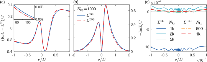
Figure 1: Self-energies $\Sigma^{\mathrm{FG}}$ and $\Sigma^{\mathrm{IFG}}$ for the single-orbital Anderson impurity model. (a) Real part (minus the Hartree shift), (b) imaginary part. The discrepancies in (a) and (b) reflect the fact that $\Sigma^{(0)}\!=\!-\frac{1}{\pi}\!\int\!\mathrm{d}\nu\,\mathrm{Im}\!\;\Sigma_{\nu}$ is exact in $\Sigma^{\mathrm{IFG}}$ but not in $\Sigma^{\mathrm{FG}}$. Indeed, the inset in (a) enlarges the high-frequency decay with the exact asymptote $\Sigma^{(0)}_{\mathrm{ex}}/\nu$ in gray. (c) $\mathrm{Im}\!\;\Sigma_{\nu}$ at low energies for an increasing number of kept states $N_{\mathrm{kp}}$ [SU(2) multiplets; $1\mathsf{k}\!=\!10^{3}$, etc.]. Crucially, $-\mathrm{Im}\!\;\Sigma^{\mathrm{IFG}}_{\nu}$ is nonnegative, free of any wiggles, and, on the given scale, converged for $N_{\mathrm{kp}}$ as low as $500$.

IV Numerical results

IV.1 NRG setting

We employ the fdm NRG Weichselbaum and von Delft (2007) in a state-of-the-art implementation based on the QSpace tensor library Weichselbaum (2012a); *Weichselbaum2012b; *Weichselbaum2020, allowing one to exploit Abelian and non-Abelian symmetries. Indeed, SU(2) spin symmetry is used throughout, while two calculations additionally have SU(2) charge and SU(3) orbital symmetry, respectively. The resolution at finite $\nu$ is improved by averaging the (discrete) spectral data over $n_{z}$ shifted discretization grids Žitko and Pruschke (2009) and through an adaptive broadening scheme Lee and Weichselbaum (2016); Lee et al. (2017). For the single-orbital results, we set the NRG discretization parameter to $\Lambda\!=\!2$ and $n_{z}\!=\!4$. For the multiorbital results, we use $\Lambda\!=\!4$ while fixing $n_{z}\!=\!2$ to reduce numerical run times. The only truncation criterion during the NRG iterative diagonalization is given by the number of kept states $N_{\mathrm{kp}}$. As usual, this bound is soft in order to respect emergent degeneracies in the spectrum.

We will first discuss the Anderson impurity model with a featureless hybridization function. All other results stem from DMFT solutions of lattice systems which are mapped onto self-consistently determined impurity models. For simplicity, we consider the Bethe lattice with a semicircular lattice density of states and converge the DMFT self-consistency iteration using the conventional self-energy scheme $\Sigma^{\mathrm{FG}}$. Although the self-consistency condition on the Bethe lattice can be phrased in terms of the spectral function $\mathcal{A}_{\alpha\nu}=-\tfrac{1}{\pi}\mathrm{Im}\!\;G_{\alpha\nu}$, it is standard practice to use the self-energy for an improved spectral function compared to the direct NRG output. Then, from the converged DMFT solution, we perform one more calculation to compare results with different self-energy estimators.

Generally, we use the half bandwidth $D=1$ of the (bare) hybridization function as our energy unit. For the plain Anderson impurity model, the size of $\Sigma$ is best compared to the hybridization strength $\Gamma$. In lattice systems, the self-energy adds to the dispersion relation in the inverse propagator; we thus plot $\Sigma/D$. For all our numerical results, we set $T/D=10^{-8}$, which can be considered as zero temperature.

IV.2 Single-orbital Anderson impurity model

We begin our presentation of numerical results with the single-orbital Anderson impurity model [cf. Eq. (2)], with a box-shaped hybridization function $-\mathrm{Im}\!\;\Delta_{\nu}=\Gamma\theta(D-|\nu|)$ of half bandwidth $D=1$ and strength $\Gamma$. We here choose $\Gamma=0.1$, an interaction value of $U=0.3$, and the on-site energy $\epsilon_{d}=-0.1$. With $\epsilon_{d}>-U/2$, the system is less than half filled, having $n_{d}=\sum_{\sigma}\langle n_{\sigma}\rangle\approx 0.87$. Appendix B provides additional results, obtained for the same parameter set as chosen in Ref. Bulla et al. (1998): $\Gamma=0.015$, $U=0.2$, and $\epsilon_{d}=-0.1$ (half filling). For the present model, $q_{\sigma}=Ud_{\sigma}n_{\bar{\sigma}}$. Hence, the Hartree self-energy gives the well-known $\Sigma^{\mathrm{H}}_{\sigma}=\langle\{q_{\sigma},d^{\dagger}_{\sigma}\}\rangle=Un_{d}/2$. Using Eq. (35), the (exact) self-energy moment is easily evaluated as $\Sigma^{(0)}_{\mathrm{ex}}\!=\!\langle\{\tilde{q}_{\sigma},\tilde{q}^{\dagger}_{\sigma}\}\rangle\!=\!U^{2}\tfrac{n_{d}}{2}(1\!-\!\tfrac{n_{d}}{2})$. Our temperature $T\!=\!10^{-8}$ is far below the Kondo temperature of $T_{\mathrm{K}}\approx 0.043$.

To set the stage, Figs. 1(a) and 1(b) show the real and imaginary part of $\Sigma$ on a wide energy window. Generally, $\Sigma^{\mathrm{FG}}_{\nu}$ and $\Sigma^{\mathrm{IFG}}_{\nu}$ yield consistent results, while slight deviations are observed at higher energies. This is expected since $\Sigma^{\mathrm{IFG}}_{\nu}$ gives the exact high-frequency asymptote for the real part [see inset of Fig. 1(a)] and the exact total weight for the imaginary part, whereas both properties are slightly violated in $\Sigma^{\mathrm{FG}}_{\nu}$. Before inspecting this further, we enlarge the low-energy behavior of $\mathrm{Im}\!\;\Sigma_{\nu}$ in Fig. 1(c) and compare results for different numbers of kept states $N_{\mathrm{kp}}$ [here SU(2) multiplets]. For $N_{\mathrm{kp}}=1000$, $-\mathrm{Im}\!\;\Sigma^{\mathrm{FG}}_{\nu}$ overshoots to negative values on the scale of $10^{-3}\Gamma$. Increasing $N_{\mathrm{kp}}$, $-\mathrm{Im}\!\;\Sigma^{\mathrm{FG}}_{\nu}$ approaches the $\nu$ axis. Importantly, however, the notable wiggles of $\mathrm{Im}\!\;\Sigma^{\mathrm{FG}}_{\nu}$ on the scale of $10^{-4}\Gamma$ remain, even for $N_{\mathrm{kp}}$ as high as $5000$. In striking contrast, $-\mathrm{Im}\!\;\Sigma^{\mathrm{IFG}}_{\nu}$ is nonnegative, free of any wiggles, and, on the given scale, already converged for $N_{\mathrm{kp}}$ as low as $500$.

In Fig. 2, we take a closer look at both the high-energy property $\Sigma^{(0)}=-\tfrac{1}{\pi}\!\int\!\mathrm{d}\nu\,\mathrm{Im}\!\;\Sigma_{\nu}$ and the low-energy property $\mathrm{Im}\!\;\Sigma_{\nu=0}$. The former should give $\Sigma^{(0)}_{\mathrm{ex}}=U^{2}\tfrac{n_{d}}{2}(1-\tfrac{n_{d}}{2})$, the latter zero at $T=0$ [or more generally $\mathit{O}(T^{2}/T_{\mathrm{K}}$)]. We plot both quantities as a function of $1/N_{\mathrm{kp}}$, i.e., with accuracy increasing toward the left. Starting with Fig. 2(a) and $\Sigma^{\mathrm{FG}}$, we see that the deviation of $\Sigma^{(0)}$ from $\Sigma^{(0)}_{\mathrm{ex}}$ decreases with increasing the number of kept states, $N_{\mathrm{kp}}$, and the number of $z$ shifts $n_{z}$. However, the relative deviation stays above $5\%$ even for the high-accuracy setting $N_{\mathrm{kp}}=5000$ and $n_{z}=4$. By contrast, for $\mathrm{Im}\!\;\Sigma^{\mathrm{IFG}}_{\nu}$ (and also $\mathrm{Im}\!\;\Sigma^{\mathrm{IF}}_{\nu}$), the exact total weight is guaranteed, no matter the chosen parameters.

As a low-energy property, $\mathrm{Im}\!\;\Sigma_{\nu=0}$, shown in Fig. 2(b), is basically independent of discretization details and thus almost the same for $n_{z}=2$ and $n_{z}=4$. One readily observes that $\mathrm{Im}\!\;\Sigma^{\mathrm{IFG}}_{\nu=0}$ is more accurate than $\mathrm{Im}\!\;\Sigma^{\mathrm{FG}}_{\nu=0}$ (and also $\mathrm{Im}\!\;\Sigma^{\mathrm{IF}}_{\nu=0}$) by several orders of magnitude. In more detail, for all self-energy estimators, the values improve (quasi) monotonically with $N_{\mathrm{kp}}$ and approach the exact value, zero. For the lower values of $N_{\mathrm{kp}}$, the numerical error in $\mathrm{Im}\!\;\Sigma^{\mathrm{IFG}}_{\nu=0}$ is dominated by $(\mathrm{Im}\!\;\Sigma^{\mathrm{FG}}_{\nu=0})^{2}$ in Eq. (30), leading to the quadratic relation between both curves in Fig. 2(b). For higher $N_{\mathrm{kp}}$ and extremely low values of $|\mathrm{Im}\!\;\Sigma^{\mathrm{IFG}}_{\nu=0}|$, uncertainties in the first two terms of Eq. (30) become noticeable. Indeed, at $N_{\mathrm{kp}}=1000$, e.g., $\Sigma^{\mathrm{FG}}$, $\Sigma^{\mathrm{IF}}$, and $\Sigma^{\mathrm{IFG}}$ roughly yield $10^{-3}$, $10^{-4}$, and $10^{-6}$, respectively. Increasing $N_{\mathrm{kp}}$ to $5000$, $-\mathrm{Im}\!\;\Sigma^{\mathrm{FG}}_{\nu=0}/\Gamma$ reaches down to $10^{-5}$ and $-\mathrm{Im}\!\;\Sigma^{\mathrm{IFG}}_{\nu=0}/\Gamma$ even down to $10^{-7}$.

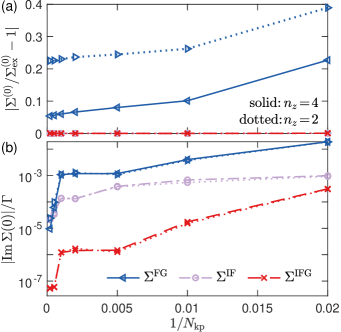
Figure 2: The self-energy moment $\Sigma^{(0)}\!=\!-\frac{1}{\pi}\!\int\!\mathrm{d}\nu\,\mathrm{Im}\!\;\Sigma_{\nu}$ and $\mathrm{Im}\!\;\Sigma_{\nu=0}$ as a function of $1/N_{\mathrm{kp}}$. (a) The $\Sigma^{\mathrm{FG}}$ results improve with increasing $N_{\mathrm{kp}}$ and $n_{z}$, the number of $z$ shifts; $\Sigma^{\mathrm{IFG}}$ (and $\Sigma^{\mathrm{IF}}$) always yield the exact value. (b) All results get closer to the exact value zero with increasing $N_{\mathrm{kp}}$ while being almost independent of $n_{z}$. Throughout, $\Sigma^{\mathrm{IFG}}$ improves upon $\Sigma^{\mathrm{FG}}$ by two to three orders of magnitude.

IV.3 Single-orbital Hubbard model

Next, we consider the DMFT+NRG solution of the single-orbital Hubbard model (Bethe lattice with half bandwidth $D=1$). We set the interaction value to $U=2.6$ in the metal–insulator coexistence region. Metallic and insulating solutions are obtained by approaching $U$ from below and above, respectively, in the DMFT self-consistency iteration. For this particle-hole symmetric setup, we exploit SU(2) charge and SU(2) spin symmetry, keeping $N_{\mathrm{kp}}=5000$ multiplets. Working with the shift $\zeta=\Sigma^{\mathrm{H}}$ (cf. Sec. III.4), we particularly have $\tilde{\Sigma}^{\mathrm{IF}}_{z}=\tilde{I}_{z}/(1+\tilde{F}_{z})$.

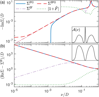
Figure 3: Self-energies for the single-orbital Hubbard model in (a) the metallic and (b) the insulating phase (see spectral functions in the insets) at $U/D\!=\!2.6$. (a) While $-\mathrm{Im}\!\;\Sigma^{\mathrm{FG}}_{\nu}$ overshoots to negative values and $-\mathrm{Im}\!\;\Sigma^{\mathrm{IF}}_{\nu}$ has artifacts when $|1\!+\!\tilde{F}_{\nu}|$ becomes small, $-\mathrm{Im}\!\;\Sigma^{\mathrm{IFG}}_{\nu}$ gives reliable results throughout. The red dotted line shows the low-energy behavior via Eq. (15) and follows the $\nu^{2}$ decay smoothly down to $-\mathrm{Im}\!\;\Sigma^{\mathrm{IFG}}_{\nu}/D\!\sim\!10^{-13}$. (b) $\mathrm{Re}\!\;\Sigma^{\mathrm{FG}}_{\nu}$ and $\mathrm{Re}\!\;\Sigma^{\mathrm{IFG}}_{\nu}$ follow the $1/\nu$ divergence of the Mott insulator, but $\mathrm{Re}\!\;\Sigma^{\mathrm{IF}}_{\nu}$ deviates from that as soon as $|1\!+\!\tilde{F}_{\nu}|$ levels off, due to inaccuracies in $\mathrm{Re}\!\;\tilde{F}_{\nu}$.

Figures 3(a) and 3(b) show $\mathrm{Im}\!\;\Sigma_{\nu}$ for the metallic solution and $\mathrm{Re}\!\;\Sigma_{\nu}$ for the insulating solution, respectively. Overall, $\Sigma^{\mathrm{FG}}$ and $\Sigma^{\mathrm{IFG}}$ give consistent results for both phases. For the metal, however, $-\mathrm{Im}\!\;\Sigma^{\mathrm{FG}}_{\nu}$ overshoots to unphysical negative values at the point $\nu\approx 2\cdot 10^{-3}$ and $-\mathrm{Im}\!\;\Sigma^{\mathrm{FG}}_{\nu}\approx 10^{-3}$, while $-\mathrm{Im}\!\;\Sigma^{\mathrm{IFG}}_{\nu}$ decreases smoothly down to $-\mathrm{Im}\!\;\Sigma_{\nu}\approx 10^{-6}$. Again, the two values are related quadratically by Eq. (30). The red dotted line in the plot gives the low-energy behavior of $\mathrm{Im}\!\;\Sigma^{\mathrm{IFG}}_{\nu}$ according to Eq. (15), i.e., by discarding the erroneous $(\mathrm{Im}\!\;\Sigma^{\mathrm{FG}}_{\nu})^{2}$ in Eq. (30). For this highly symmetric (and highly accurate) calculation, the result goes smoothly down in energy, all the way to $-\mathrm{Im}\!\;\Sigma^{\mathrm{IFG}}_{\nu}/D\!\sim\!10^{-13}$.

Turning to $\Sigma^{\mathrm{IF}}$ in Fig. 3(a), the curve also shows a clean $\nu^{2}$ decay, but it has a peculiar dip at larger frequencies, $\nu\approx 0.2$. The reason is that the spectral function in the metallic phase (see inset) exhibits strongly reduced weight at precisely these frequencies, separating the quasiparticle peak from the Hubbard bands. This leads to low values in $|1+\tilde{F}_{\nu}|$ (as explained in Sec. III.5) and artifacts in $\Sigma^{\mathrm{IF}}_{\nu}$. In the insulating phase, Fig. 3(b), $\mathrm{Re}\!\;\Sigma^{\mathrm{FG}}$ and $\mathrm{Re}\!\;\Sigma^{\mathrm{IFG}}$ nicely follow the $1/\nu$ divergence of the Mott insulator. There, $|1+\tilde{F}_{\nu}|$ should decrease to zero for $\nu\to 0$. However, due to inaccuracies in the real part obtained by Kramers–Kronig transform, $|1+\tilde{F}_{\nu}|$ levels off for $\nu<0.01$, so that $\mathrm{Re}\!\;\Sigma^{\mathrm{IF}}_{\nu}$ deviates from $1/\nu$. In total, for this strongly correlated setup, $\Sigma^{\mathrm{IF}}$ does not give reliable results since the denominator $1+\tilde{F}_{\nu}$ leads to numerical instabilities.

IV.4 Multiorbital Hubbard models

We now turn to DMFT+NRG results for multiorbital Hubbard models on the Bethe lattice with the interaction given by Eq. (3). We first consider two half-filled orbitals and different bandwidths of $D\equiv D_{1}=1$ and $D_{2}=0.5$. Setting $U=1.8$ and $J=0.3$ yields a simple realization of an orbital-selective Mott phase (OSMP). Indeed, in the absence of interorbital hopping Kugler and Kotliar , the 1-orbital is metallic while the 2-orbital is a Mott insulator with a gap in the spectrum (see inset of Fig. 4). Note that, for the present calculation, the Wilson chains of the two orbitals are interleaved Mitchell et al. (2014); Stadler et al. (2016) for extra efficiency.

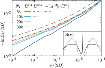
Figure 4: Self-energies $\Sigma_{1}$ of the metallic orbital in a two-orbital realization of the OMSP (see spectral functions in the inset). As a singular Fermi liquid, $-\mathrm{Im}\!\;\Sigma_{1,\nu}$ is expected to show a logarithmic singularity. With $\Sigma^{\mathrm{FG}}$, this behavior is only seen for the largest $N_{\mathrm{kp}}$. By contrast, $\mathrm{Im}\!\;\Sigma^{\mathrm{IFG}}_{1,\nu}$ perfectly agrees with the analytic curve and is, on the given scale, already converged for the lowest $N_{\mathrm{kp}}=5000$. The extra factor $2$ on the axes is used to have convenient tick marks.

The main panel of Fig. 4 shows the self-energy of the metallic 1-orbital, $\Sigma_{1}$, at low energies and for various $N_{\mathrm{kp}}$. It is known that, due to the unscreened magnetic moments of the 2-orbital, the 1-orbital is a singular Fermi liquid with logarithmic singularities in $\Sigma_{1}$ Greger et al. ; Kugler et al. (2019). The black dashed line shows the expected $a\ln^{-2}|\nu/T^{*}|$ behavior; where $a$ and $T^{*}$ are fitting parameters. We multiplied $a$ by an extra factor $1.2$ to separate the curves for better readability. The numerical data obtained with $\Sigma^{\mathrm{FG}}$ shifts notably by increasing $N_{\mathrm{kp}}$ from 5000 to 30000 SU(2) multiplets. For the lowest accuracy, $\mathrm{Im}\!\;\Sigma^{\mathrm{FG}}_{1,\nu}$ does not reproduce the analytically expected behavior and still contains notable wiggles. Increasing $N_{\mathrm{kp}}$, $\mathrm{Im}\!\;\Sigma^{\mathrm{FG}}_{1,\nu}$ approaches the expected behavior but is not fully converged at $N_{\mathrm{kp}}=30000$. By contrast, $\Sigma^{\mathrm{IFG}}$ always yields a stable curve, in excellent agreement with the analytic form, and is, on the given scale, already converged for the lowest number of kept states, $N_{\mathrm{kp}}=5000$.

We close our presentation of numerical results with a three-orbital setup of the Hund-metal category Haule and Kotliar (2009); Georges et al. (2013). Having three degenerate orbitals, we exploit the additional SU(3) symmetry permitted by Eq. (3). There, we set $U=3$, $J=0.5$ in units of the half bandwidth $D=1$. At a filling of two, the spectral function (see inset of Fig. 5) is highly asymmetric. The left part of $\mathcal{A}_{\nu}$ exhibits an intriguing orbital-resonance shoulder Stadler et al. (2016, 2019); Kugler et al. (2019), and we thus focus on $\nu<0$ for the analysis of $\Sigma$.

Figure 5 shows $|\mathrm{Im}\!\;\Sigma_{\nu}|$ for both estimators $\Sigma^{\mathrm{FG}}$ and $\Sigma^{\mathrm{IFG}}$ and for $N_{\mathrm{kp}}=3000$, $4000$, and $5000$ SU(2)$\times$SU(3) multiplets. In this challenging, three-orbital setup, $-\mathrm{Im}\!\;\Sigma^{\mathrm{FG}}_{\nu}$ overshoots to unphysical negative values already at the point where $-\nu$ and $-\mathrm{Im}\!\;\Sigma$ are around $10^{-2}$. For $\Sigma^{\mathrm{FG}}$ calculations with higher $N_{\mathrm{kp}}$, this point is shifted only marginally to lower $\nu$. Wiggles in $\mathrm{Im}\!\;\Sigma^{\mathrm{FG}}_{\nu}$ are on the scale of $10^{-3}$ for the lower $N_{\mathrm{kp}}$ and weaker but still present for the largest $N_{\mathrm{kp}}$. Again, $\Sigma^{\mathrm{IFG}}$ eradicates the overshooting problem. Even for the lowest $N_{\mathrm{kp}}$, $-\mathrm{Im}\!\;\Sigma^{\mathrm{IFG}}_{\nu}$ follows a clean $\nu^{2}$ decay down to values of $10^{-3}$, before wiggles appear on the scale of $10^{-4}$. For the highest $N_{\mathrm{kp}}=5000$, $-\mathrm{Im}\!\;\Sigma^{\mathrm{IFG}}_{\nu}$ follows the $\nu^{2}$ decay down to values of $10^{-4}$ and hardly any wiggles are to be found. Again, the values of $|\mathrm{Im}\!\;\Sigma^{\mathrm{FG}}_{\nu=0}|$ and $|\mathrm{Im}\!\;\Sigma^{\mathrm{IFG}}_{\nu=0}|$ relate quadratically [Eq. (30)]. The red dotted line shows $\mathrm{Im}\!\;\Sigma^{\mathrm{IFG}}_{\nu}$ for $|\nu|\to 0$ according to Eq. (15) and reaches down to values of $-\mathrm{Im}\!\;\Sigma^{\mathrm{IFG}}_{\nu}/D\sim 10^{-6}$.

It is clear from the plot that converging the standard estimator $\Sigma^{\mathrm{FG}}$ with $N_{\mathrm{kp}}$ toward a clean $\nu^{2}$ decay down to, say, $10^{-3}$ is very slow and practically unfeasible. By contrast, $\Sigma^{\mathrm{IFG}}$ gives very accurate results already for much lower $N_{\mathrm{kp}}$, and its low-energy behavior can be extracted very cleanly from Eq. (15). We hope that, in this way, our new self-energy estimator will expand the class of systems where NRG can be used as a highly-accurate, real-frequency DMFT impurity solver.

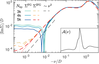
Figure 5: Self-energies in a degenerate three-orbital Hund-metal system. We focus on negative frequencies where the spectral function at filling $2$ has a pronounced shoulder (see inset). $-\mathrm{Im}\!\;\Sigma^{\mathrm{FG}}_{\nu}$ overshoots to unphysical negative values for $-\nu/D\!\lesssim\!10^{-2}$ for all numerically feasible $N_{\mathrm{kp}}$ [SU(2)$\times$SU(3) multiplets]. By contrast, $-\mathrm{Im}\!\;\Sigma^{\mathrm{IFG}}_{\nu}$ never overshoots and follows the $\nu^{2}$ decay down to $-\mathrm{Im}\!\;\Sigma^{\mathrm{IFG}}_{\nu}/D\!=\!10^{-3}$ and even $10^{-4}$ for $N_{\mathrm{kp}}\!=\!3000$ and $5000$, respectively. The red dotted line shows the low-energy behavior according to Eq. (15) and follows the $\nu^{2}$ decay smoothly down to $-\mathrm{Im}\!\;\Sigma^{\mathrm{IFG}}_{\nu}/D\sim 10^{-6}$.

V Conclusion

We presented a new self-energy estimator and showed that it yields greatly improved results in NRG calculations. The standard estimator $\Sigma^{\mathrm{FG}}=F/G$ [see Eqs. (5) and (11)] follows from an eom for $G$. While it yields much better results than employing the Dyson equation, $\Sigma^{\mathrm{FG}}$ still does not have all the qualities one is used to from fdm NRG correlators, as $\mathrm{Im}\!\;\Sigma^{\mathrm{FG}}$ is not properly normalized and can overshoot to positive values. Moreover, it often displays wiggles for very low energies.

By combining the eom for $G$ with an analogous eom for $F$, one can derive several $\Sigma$ estimators [see Eqs. (23)–(27)]. We identified $\Sigma^{\mathrm{IFG}}=\Sigma^{\mathrm{H}}+I-F^{2}/G$ as particularly well-suited for NRG. Indeed, we showed analytically that the normalization of $\mathrm{Im}\!\;\Sigma^{\mathrm{IFG}}$ [Eq. (14)] and its low-energy behavior [see Eq. (15)] are determined directly by $\mathrm{Im}\!\;I$, $\mathrm{Im}\!\;F$, and $\mathrm{Im}\!\;G$. Accordingly, there are no real parts (obtained by Kramers–Kronig transform) involved, and $\mathrm{Im}\!\;\Sigma^{\mathrm{IFG}}$ is as reliable as the imaginary part of any fdm NRG correlator: it is normalized, does not overshoot, and is extremely accurate at low energies.

We examined numerical results for the Anderson impurity model with a featureless hybridization and for the DMFT solutions of one-, two-, and three-orbital Hubbard models. In all cases, the above properties were confirmed and $\Sigma^{\mathrm{IFG}}$ yielded much better results than $\Sigma^{\mathrm{FG}}$. Furthermore, we found that $\Sigma^{\mathrm{IFG}}$ converged much faster with increasing the numerical effort (increasing the number of kept states $N_{\mathrm{kp}}$) than $\Sigma^{\mathrm{FG}}$. This is very important when applying NRG to multiorbital systems where the maximal $N_{\mathrm{kp}}$ is limited by numerical resources and finding accurate results for $\Sigma^{\mathrm{FG}}$ was the major challenge.

The estimator $\Sigma^{\mathrm{FG}}=F/G$ is also frequently used for other impurity solvers, such as exact diagonalization (ED) N. Enenkel et al. , the density-matrix renormalization group (DMRG) Zhu et al. (2017); Karp et al. (2020) and quantum Monte Carlo (QMC) Hafermann et al. (2012, 2013); Hafermann (2014); Gunacker et al. (2016). Although our analysis is targeted at NRG applications, we expect that $\Sigma^{\mathrm{IFG}}$ yields improved results for some of these methods, too.

Appendix A Matrix-valued correlation functions

In the main text, we focused on $\alpha$-diagonal fermionic correlation functions, as they follow from Eqs. (1)–(3). Matrix-valued correlation functions are obtained if the quadratic Hamiltonian is generalized to

$$H_{0} =\textstyle\sum_{\alpha\alpha^{\prime}}d^{\dagger}_{\alpha^{\prime}}\epsilon_{d,\alpha^{\prime}\alpha}d_{\alpha}+\sum_{k,\alpha\alpha^{\prime}}c^{\dagger}_{k\alpha^{\prime}}\epsilon_{k,\alpha^{\prime}\alpha}c_{k\alpha}$$

$$\ \textstyle+\sum_{k,\alpha\alpha^{\prime}}(d_{\alpha^{\prime}}^{\dagger}V_{k,\alpha^{\prime}\alpha}c_{k\alpha}+\mathrm{H.c.})$$ (39)

and has nonzero off-diagonal ($\alpha\!\neq\!\alpha^{\prime}$) elements. Indeed, this expression contains several matrices, which we denote by $\epsilon_{d}$, $\epsilon_{k}$, and $V_{k}$ without subscripts $\alpha$. Most results of the main text are purposefully phrased in such a way that they directly generalize to matrix form upon removing $\alpha$ indices. An exception is the hybridization function in Eq. (8), which is rephrased as

$$\textstyle\Delta_{z}=\sum_{k}V_{k}(z-\epsilon_{k})^{-1}V^{\dagger}_{k}.$$ (40)

The matrix-valued correlation functions are denoted by $G_{z}$, $I_{z}$, etc., without $\alpha$ indices. Their matrix elements are defined by

$$\quad G_{\alpha\alpha^{\prime},z} =\langle\mspace{-3.0mu}\langle d_{\alpha},d_{\alpha^{\prime}}^{\dagger}\rangle\mspace{-3.0mu}\rangle_{z},\quad I_{\alpha\alpha^{\prime},z} =\langle\mspace{-3.0mu}\langle q_{\alpha},q_{\alpha^{\prime}}^{\dagger}\rangle\mspace{-3.0mu}\rangle_{z},$$ (41)

$$\quad F^{\mathrm{L}}_{\alpha\alpha^{\prime},z} =\langle\mspace{-3.0mu}\langle q_{\alpha},d_{\alpha^{\prime}}^{\dagger}\rangle\mspace{-3.0mu}\rangle_{z},\quad F^{\mathrm{R}}_{\alpha\alpha^{\prime},z} =\langle\mspace{-3.0mu}\langle d_{\alpha},q_{\alpha^{\prime}}^{\dagger}\rangle\mspace{-3.0mu}\rangle_{z}.$$ (42)

In this generalized setting, too, one computes with NRG the Lehmann representation of a spectral function like

$$\mathcal{A}^{\mathrm{G}}_{\nu} =(G_{\nu}-G_{\nu}^{\dagger})/(-2\pi\mathrm{i}).$$ (43)

Its diagonal elements fulfill the standard relation $\mathcal{A}^{\mathrm{G}}_{\alpha\alpha,\nu}\!=\!-\frac{1}{\pi}\mathrm{Im}\!\;G_{\alpha\alpha,\nu}$, while the off-diagonal elements are generally complex. From the Lehmann representation, one also finds $\mathcal{A}^{\mathrm{F}^{\mathrm{L}}}_{\nu}\!=\!(\mathcal{A}^{\mathrm{F}^{\mathrm{R}}}_{\nu})^{\dagger}$ as the generalization of $F^{\mathrm{L}}_{\alpha\alpha,z}\!=\!F^{\mathrm{R}}_{\alpha\alpha,z}$ used in the main text. The retarded correlator subsequently follows as

$$G_{\nu}=\,\mathcal{P}\!\!\int\!\mathrm{d}\nu^{\prime}\frac{1}{\nu-\nu^{\prime}}\mathcal{A}^{\mathrm{G}}_{\nu^{\prime}}\,-\,\mathrm{i}\pi\mathcal{A}^{\mathrm{G}}_{\nu}.$$ (44)

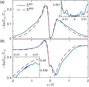
Figure 6: Imaginary part of two self-energy components for the Anderson impurity model with off-diagonal on-site energy and hybridization. For both a diagonal (a) and off-diagonal (b) element of $\Sigma$, the results from $\Sigma^{\mathrm{IFG}}$ are smoother than those of $\Sigma^{\mathrm{FG}}$ and free from wiggles at low energies. The total weight $\int\mathrm{d}\nu\mathcal{A}^{\Sigma}_{\nu}$ from $\Sigma^{\mathrm{IFG}}$ is in perfect agreement with the exact value $\langle\{\tilde{q}_{\alpha},\tilde{q}^{\dagger}_{\alpha^{\prime}}\}\rangle$, cf. Eq. (35), whereas that obtained with $\Sigma^{\mathrm{FG}}$ deviates by roughly 15% in each component.

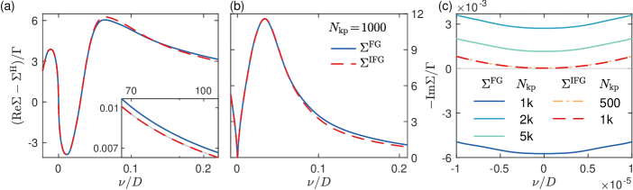
Figure 7: Self-energies $\Sigma^{\mathrm{FG}}$ and $\Sigma^{\mathrm{IFG}}$ for the single-orbital Anderson impurity model, as in Fig. 1, but at a stronger interaction, $\Gamma/U=0.075$, and half filling. (a) Real part (minus the Hartree shift) and (b) imaginary part on a wide frequency window. Discrepancies reflect the fact that $\Sigma^{(0)}$ is exact in $\Sigma^{\mathrm{IFG}}$ but not in $\Sigma^{\mathrm{FG}}$. We restrict the frequency range to $\nu>0$ in light of particle-hole symmetry. The inset in (a) enlarges the high-frequency decay with $\Sigma^{(0)}_{\mathrm{ex}}/\nu$ in gray. (c) $\mathrm{Im}\!\;\Sigma_{\nu}$ at low energies for an increasing number of kept states $N_{\mathrm{kp}}$ [SU(2)$\times$SU(2) multiplets]. One observes that $-\mathrm{Im}\!\;\Sigma^{\mathrm{FG}}_{\nu}$ overshoots to negative values for $N_{\mathrm{kp}}=1000$ and is not yet converged for the highest $N_{\mathrm{kp}}=5000$. By contrast, $-\mathrm{Im}\!\;\Sigma^{\mathrm{IFG}}_{\nu}$ shows a clean, nonnegative parabola and is, on the given scale, converged for $N_{\mathrm{kp}}$ as low as $500$.

The equations of motion (19) and (21) involving $F^{\mathrm{L}}$, together with their counterparts involving $F^{\mathrm{R}}$, were already given in a way that directly generalizes to matrix form. The same applies to the $\Sigma$ formulas (22)–(27) if $F$ without superscript is understood as $F^{\mathrm{L}}$. Here, we gather the various matrix-valued $\Sigma$ estimators in both their “left” and “right” forms:

$$\Sigma^{\mathrm{FG}}_{z} =F_{z}^{\mathrm{L}}G_{z}^{-1}$$ (45a)

$$=G_{z}^{-1}F_{z}^{\mathrm{R}},$$ (45b)

$$\Sigma^{\mathrm{IG}}_{z} =(\Sigma^{\mathrm{H}}+I_{z})G^{0}_{z}G_{z}^{-1}$$ (45c)

$$=G_{z}^{-1}G^{0}_{z}(\Sigma^{\mathrm{H}}+I_{z}),$$ (45d)

$$\Sigma^{\mathrm{I}}_{z} =[1+(\Sigma^{\mathrm{H}}+I_{z})G^{0}_{z}]^{-1}(\Sigma^{\mathrm{H}}+I_{z})$$ (45e)

$$=(\Sigma^{\mathrm{H}}+I_{z})[1+G^{0}_{z}(\Sigma^{\mathrm{H}}+I_{z})]^{-1},$$ (45f)

$$\Sigma^{\mathrm{IF}}_{z} =(1+F^{\mathrm{L}}_{z})^{-1}(\Sigma^{\mathrm{H}}+I_{z})$$ (45g)

$$=(\Sigma^{\mathrm{H}}+I_{z})(1+F^{\mathrm{R}}_{z})^{-1},$$ (45h)

$$\Sigma^{\mathrm{IFG}}_{z} =\Sigma^{\mathrm{H}}+I_{z}-F^{\mathrm{L}}_{z}G_{z}^{-1}F^{\mathrm{R}}_{z}.$$ (45i)

Note that the last term can also be written as $(F^{\mathrm{L}}_{z})^{2}G_{z}^{-1}$, $G_{z}^{-1}(F^{\mathrm{R}}_{z})^{2}$. However, this spoils the invariance under shifts (see Sec. III.4) and is therefore numerically disadvantageous.

Finally, we present an exemplary set of numerical results for matrix-valued self-energies. We consider an Anderson impurity model, similar to the one from Sec. IV.2, with a boxed-shaped hybridization function $\mathcal{A}^{\Delta}_{\nu}=\Gamma\theta(D-|\nu|)/\pi$, and interaction strength $U=0.3$ and temperature $T=10^{-8}$ in units of the half bandwidth $D=1$. However, differently from Sec. IV.2, we promote the on-site energy $\epsilon_{d}$ and the hybridization strength $\Gamma$ to non-diagonal matrices:

$$\epsilon_{d}=\begin{pmatrix}-0.2&0.05\mathrm{i}\\ -0.05\mathrm{i}&-0.1\end{pmatrix},\qquad\Gamma=\begin{pmatrix}1&-\mathrm{i}\\ \mathrm{i}&\phantom{+}1\end{pmatrix}.$$ (46)

This model exhibits only a U(1) charge symmetry, and we choose the NRG parameters as $\Lambda=2$, $n_{z}=2$, $N_{\mathrm{kp}}=8000$. The self-energies $\Sigma^{\mathrm{FG}}$ and $\Sigma^{\mathrm{IFG}}$ are obtained from their matrix expressions (45a) and (45i). Figure 6 shows the imaginary part of two exemplary components, $\Sigma_{11}$ and $\Sigma_{21}$. Overall, both estimators yield consistent results. However, already on the wide frequency window, one observes that $\Sigma^{\mathrm{IFG}}$ results are much smoother than those of $\Sigma^{\mathrm{FG}}$. The notable differences at large energies owe to the fact that $\Sigma^{\mathrm{IFG}}$ produces the exact total weight $\int\mathrm{d}\nu\mathcal{A}^{\Sigma}_{\nu}$ as known from $\langle\{\tilde{q}_{\alpha},\tilde{q}^{\dagger}_{\alpha^{\prime}}\rangle$ expectation values, cf. Eq. (35), while the corresponding results from $\Sigma^{\mathrm{FG}}$ deviate by roughly 15% in each component. The insets, enlarging the low-energy regime, reveal that, also in the non-diagonal setting, $\Sigma^{\mathrm{IFG}}$ is free from the wiggles present in $\Sigma^{\mathrm{FG}}$. Remarkably, this applies not only to the diagonal self-energy component where the imaginary part vanishes at $\nu=0$, but also to the off-diagonal component where this value is finite.

Appendix B Anderson impurity model at strong interaction

Here, we give additional numerical results for the ($\alpha$-diagonal) single-orbital Anderson impurity model at strong interaction. We choose the same parameter set as in Ref. Bulla et al. (1998): a box-shaped hybridization function of half bandwidth $D=1$ and strength $\Gamma=0.015$, an interaction value of $U=0.2$, and $\epsilon_{d}=-0.1$ corresponding to half filling. The particle-hole symmetry allows us to exploit SU(2) charge and SU(2) spin symmetry in the calculation, as already done in Sec. IV.3. We set $\Lambda=2$ and $n_{z}=4$ as in Sec. IV.2. The temperature $T=10^{-8}$ is again far below the Kondo temperature of $T_{\mathrm{K}}\approx 2.06\cdot 10^{-4}$, following from the same formula as used in Sec. IV.2.

Figure 7 is analogous to Fig. 1; we restrict panels (a) and (b) to positive frequencies in light of particle-hole symmetry. The findings from Sec. IV.2 also hold analogously in the current setting at strong interaction: $\Sigma^{\mathrm{FG}}$ and $\Sigma^{\mathrm{IFG}}$ are overall consistent; deviations at large frequencies in Figs. 7(a) and 7(b) reflect the fact that the high-frequency asymptote in the real part and the total weight in the imaginary part are exactly fulfilled by $\Sigma^{\mathrm{IFG}}_{\nu}$, whereas this is not the case for $\Sigma^{\mathrm{FG}}_{\nu}$. The agreement between $\mathrm{Re}\!\;\Sigma^{\mathrm{IFG}}_{\nu}$ and $\Sigma^{(0)}_{\mathrm{ex}}/\nu$ for large $\nu$ can be seen in the inset of Fig. 7(a).

The low-energy behavior of $\mathrm{Im}\!\;\Sigma_{\nu}$ for an increasing number of kept states $N_{\mathrm{kp}}$ [SU(2)$\times$SU(2) multiplets] is compared in Fig. 7(c). The wiggles of $\mathrm{Im}\!\;\Sigma^{\mathrm{FG}}_{\nu}$ at low energies, as for instance observed in Fig. 1(c), are absent in this particle-hole symmetric setting. However, for $N_{\mathrm{kp}}=1000$, $-\mathrm{Im}\!\;\Sigma^{\mathrm{FG}}_{\nu}$ still overshoots to negative values on the scale of $10^{-3}\Gamma$. Increasing $N_{\mathrm{kp}}$ to $2000$ and $5000$, $-\mathrm{Im}\!\;\Sigma^{\mathrm{FG}}_{\nu}$ continues to shift: it comes closer to the $\nu$ axis without fully reaching it, violating $\mathrm{Im}\!\;\Sigma^{\mathrm{FG}}(0)=0$ with errors on the order of $10^{-3}\Gamma$. By contrast, $-\mathrm{Im}\!\;\Sigma^{\mathrm{IFG}}_{\nu}$ shows a clean, nonnegative parabola which, on the given scale, has its vertex right at the origin and is converged for $N_{\mathrm{kp}}$ as low as $500$.

References

- Hanson et al. (2007) R. Hanson, L. P. Kouwenhoven, J. R. Petta, S. Tarucha, and L. M. K. Vandersypen, Rev. Mod. Phys. 79, 1217 (2007).
- Georges et al. (1996) A. Georges, G. Kotliar, W. Krauth, and M. J. Rozenberg, Rev. Mod. Phys. 68, 13 (1996).
- Wilson (1975) K. G. Wilson, Rev. Mod. Phys. 47, 773 (1975).
- Bulla et al. (2008) R. Bulla, T. A. Costi, and T. Pruschke, Rev. Mod. Phys. 80, 395 (2008).
- Bulla (1999) R. Bulla, Phys. Rev. Lett. 83, 136 (1999).
- Bulla et al. (2001) R. Bulla, T. A. Costi, and D. Vollhardt, Phys. Rev. B 64, 045103 (2001).
- Deng et al. (2013) X. Deng, J. Mravlje, R. Žitko, M. Ferrero, G. Kotliar, and A. Georges, Phys. Rev. Lett. 110, 086401 (2013).
- Lee et al. (2017) S.-S. B. Lee, J. von Delft, and A. Weichselbaum, Phys. Rev. Lett. 119, 236402 (2017).
- Vučičević et al. (2019) J. Vučičević, J. Kokalj, R. Žitko, N. Wentzell, D. Tanasković, and J. Mravlje, Phys. Rev. Lett. 123, 036601 (2019).
- Vranić et al. (2020) A. Vranić, J. Vučičević, J. Kokalj, J. Skolimowski, R. Žitko, J. Mravlje, and D. Tanasković, Phys. Rev. B 102, 115142 (2020).
- Vučičević and Žitko (2021a) J. Vučičević and R. Žitko, Phys. Rev. Lett. 127, 196601 (2021a).
- Vučičević and Žitko (2021b) J. Vučičević and R. Žitko, Phys. Rev. B 104, 205101 (2021b).
- Pruschke and Bulla (2005) T. Pruschke and R. Bulla, Eur. Phys. J. B 44, 217 (2005).
- Peters and Pruschke (2010a) R. Peters and T. Pruschke, Phys. Rev. B 81, 035112 (2010a).
- Peters and Pruschke (2010b) R. Peters and T. Pruschke, J. Phys. Conf. Ser. 200, 012158 (2010b).
- Peters et al. (2011) R. Peters, N. Kawakami, and T. Pruschke, Phys. Rev. B 83, 125110 (2011).
- Greger et al. (2013) M. Greger, M. Kollar, and D. Vollhardt, Phys. Rev. Lett. 110, 046403 (2013).
- (18) M. Greger, M. Sekania, and M. Kollar, arXiv:1312.0100 .
- (19) F. B. Kugler and G. Kotliar, arXiv:2112.14691 .
- Stadler et al. (2016) K. M. Stadler, A. K. Mitchell, J. von Delft, and A. Weichselbaum, Phys. Rev. B 93, 235101 (2016).
- Stadler et al. (2019) K. M. Stadler, G. Kotliar, A. Weichselbaum, and J. von Delft, Ann. Phys. 405, 365 (2019).
- Kugler et al. (2019) F. B. Kugler, S.-S. B. Lee, A. Weichselbaum, G. Kotliar, and J. von Delft, Phys. Rev. B 100, 115159 (2019).
- Stadler et al. (2021) K. M. Stadler, G. Kotliar, S.-S. B. Lee, A. Weichselbaum, and J. von Delft, Phys. Rev. B 104, 115107 (2021).
- Kugler et al. (2020) F. B. Kugler, M. Zingl, H. U. R. Strand, S.-S. B. Lee, J. von Delft, and A. Georges, Phys. Rev. Lett. 124, 016401 (2020).
- Peters et al. (2006) R. Peters, T. Pruschke, and F. B. Anders, Phys. Rev. B 74, 245114 (2006).
- Weichselbaum and von Delft (2007) A. Weichselbaum and J. von Delft, Phys. Rev. Lett. 99, 076402 (2007).
- Bulla et al. (1998) R. Bulla, A. C. Hewson, and T. Pruschke, J. Phys.: Condens. Matter 10, 8365 (1998).
- Žitko and Pruschke (2009) R. Žitko and T. Pruschke, Phys. Rev. B 79, 085106 (2009).
- Lee and Weichselbaum (2016) S.-S. B. Lee and A. Weichselbaum, Phys. Rev. B 94, 235127 (2016).
- Kaufmann et al. (2019) J. Kaufmann, P. Gunacker, A. Kowalski, G. Sangiovanni, and K. Held, Phys. Rev. B 100, 075119 (2019).
- Anderson (1961) P. W. Anderson, Phys. Rev. 124, 41 (1961).
- Dworin and Narath (1970) L. Dworin and A. Narath, Phys. Rev. Lett. 25, 1287 (1970).
- Georges et al. (2013) A. Georges, L. de’ Medici, and J. Mravlje, Annu. Rev. Condens. Matter Phys. 4, 137 (2013).
- Hafermann et al. (2012) H. Hafermann, K. R. Patton, and P. Werner, Phys. Rev. B 85, 205106 (2012).
- Moutenet et al. (2018) A. Moutenet, W. Wu, and M. Ferrero, Phys. Rev. B 97, 085117 (2018).
- Note (1) We note that requires only one correlator, , instead of the two needed for . Yet, with the same trick that led from Eq. (23\@@italiccorr) to (24\@@italiccorr), we can transform Eq. (22\@@italiccorr) to . This result, too, involves only a single full correlator. However, we numerically found to be less accurate than and hence do not discuss it any further.
- Note (2) One can also use the numerical result obtained for and substitute it on the right of Eq. (30\@@italiccorr) instead of . This yields a notable improvement at low energies but spoils high-energy properties such as the normalization of . Using Eq. (30\@@italiccorr) with on the right and solving the quadratic equation for did not turn out to be helpful.
- (38) N. Enenkel et al., unpublished.
- Note (3) In NRG, the value of may slightly differ among shifts. Using a -dependent shift makes each term consistently obey and slightly improves results.
- Luttinger (1961) J. M. Luttinger, Phys. Rev. 121, 942 (1961).
- Weichselbaum (2012a) A. Weichselbaum, Ann. Phys. 327, 2972 (2012a).
- Weichselbaum (2012b) A. Weichselbaum, Phys. Rev. B 86, 245124 (2012b).
- Weichselbaum (2020) A. Weichselbaum, Phys. Rev. Research 2, 023385 (2020).
- Note (4) Here, we use the well-known formula Haldane (1978); Merker et al. (2012) for the Kondo temperature .
- Haldane (1978) F. D. M. Haldane, Phys. Rev. Lett. 40, 416 (1978).
- Merker et al. (2012) L. Merker, A. Weichselbaum, and T. A. Costi, Phys. Rev. B 86, 075153 (2012).
- Mitchell et al. (2014) A. K. Mitchell, M. R. Galpin, S. Wilson-Fletcher, D. E. Logan, and R. Bulla, Phys. Rev. B 89, 121105 (2014).
- (48) M. Greger, M. Sekania, and M. Kollar, arXiv:1312.0100 .
- Haule and Kotliar (2009) K. Haule and G. Kotliar, New J. Phys. 11, 025021 (2009).
- Zhu et al. (2017) W. Zhu, D. N. Sheng, and J.-X. Zhu, Phys. Rev. B 96, 085118 (2017).
- Karp et al. (2020) J. Karp, M. Bramberger, M. Grundner, U. Schollwöck, A. J. Millis, and M. Zingl, Phys. Rev. Lett. 125, 166401 (2020).
- Hafermann et al. (2013) H. Hafermann, P. Werner, and E. Gull, Comput. Phys. Commun. 184, 1280 (2013).
- Hafermann (2014) H. Hafermann, Phys. Rev. B 89, 235128 (2014).
- Gunacker et al. (2016) P. Gunacker, M. Wallerberger, T. Ribic, A. Hausoel, G. Sangiovanni, and K. Held, Phys. Rev. B 94, 125153 (2016).