BPS equations and solutions for Maxwell-scalar theory

Abstract

Energy minimizing BPS equations and solutions are obtained for a class of models in Maxwell-scalar theory, where an abelian electric charge is immersed in an effective dielectric of a real scalar field. The first order BPS equations are developed using the straightforward “on-shell method” introduced by Atmaja and Ramadhan. Employment of an auxiliary function of the scalar field allows a scalar potential that displays a tachyonic instability. Consequently, a nontopological scalar soliton is found to form around the charge. Examples and solutions are provided for (1) a point charge or sphere in a flat Minkowski background, and (2) an “overcharged” compact object in a Reissner-Nordstrom background. The solutions presented here for the former (Minkowski) case recover those that have been previously obtained, while the latter solutions are new BPS solutions.

I Introduction

The possibility exists that elementary scalar fields may permeate the universe. Such scalars could have many possible origins, such as those that arise from scalar-tensor or tensor-multiscalar theories, extra dimensional theories, or string theories. At any rate, it is important to investigate possible interactions that scalar fields may have with known Standard Model fields. These interactions may be of new, possibly noncanonical form. Cvetic and Tseytlin Cvetic NPB94 have pointed out that a coupling of scalar fields to the Maxwell field and kinetic terms of nonabelian gauge fields is a generic feature of Kaluza-Klein and string theories. There, solutions have been obtained for cases where only one scalar field contributes to the action, as well as for cases where two scalar fields (dilaton and modulus) are present. It is assumed that the flat spacetime solutions approximate the exact solutions for the set of equations including gravity in regions where the curvature is small. Other studies, such as those in BBFR 03 -Brito EPJC14 have considered the effects of a dielectric medium, comprised of real (or complex) Issifu AHEP21 scalar fields coupled to abelian and/or nonabelian gauge fields. Such couplings permit new effects to emerge, including those that allow confining mechanisms.

Presently, attention is focused upon Maxwell-scalar theory, wherein a neutral scalar field $\phi$ couples nonminimally to the Maxwell field $F_{\mu\nu}$ via an “effective permittivity” coupling function $\varepsilon(r,\phi)$, which here, is allowed to develop a tachyonic instability that can result in a scalarization of an electric charge immersed in this scalar field. These types of solitonic structures have been recently investigated by Herdeiro, Oliveira, and Radu Herdeiro EPJC20 and by Bazeia, Marques, and Menezes in Bazeia EPJC21 for the case of a point charge immersed in a real scalar field, with the scalar-Maxwell interaction described by the coupling $-\frac{1}{4}\varepsilon(\phi)F_{\mu\nu}F^{\mu\nu}$. In those studies, energy minimizing first order Bogomolnyi equations and solutions were obtained for a Minkowski background, describing static, radially symmetric, charged solitonic objects. (See, e.g., Refs. Bogol 76 and Prasad PRL75 for classical papers on the subject of Bogomolnyi equations and “BPS” solutions.) Spherically symmetric static solutions for first order (Bogomolnyi) equations for the field $\phi(r)$, along with the electric field $\mathbf{E}(r)$ were found by minimizing the system energy. The resulting system describes a point charge surrounded by a scalar cloud. The presence of the scalar cloud allows the description of a new type of soliton with electric charge, and has an effect that modifies the electric field from that of Maxwell theory without the nonminimal coupling.

The methods used in Refs.Herdeiro EPJC20 and Bazeia EPJC21 work well for the case of spherical symmetry in a flat spacetime, where one can perform first integrations to obtain Bogomolnyi equations. For example, in Ref.Herdeiro EPJC20 a coordinate $x=1/r$ is defined, yielding a first integral for the equation of motion for the scalar field $\phi$. One can then, in principle, solve for $x(\phi)$, then invert to get $\phi(x)$ and transform to get $\phi(r)$. With an assumed form for $\varepsilon(\phi)$, the functions $\phi(r)$, $\varepsilon(r)$, and $\mathbf{E}(r)$ can be calculated. The authors of Ref.Herdeiro EPJC20 then proceed by considering the situation in a curved spacetime, and introduce a method of calculating the functions $\phi(r)$, $\varepsilon(r)$, and $\mathbf{E}(r)$ with perturbation theory.

The method for obtaining Bogomolnyi equations used here appears to be more direct, and follows that introduced by Atmaja and Ramadhan Atmaja PRD14 , which in the present case, is quite simple to apply. Moreover, it can be extended to accommodate the more general situation of a macroscopic compact object in a Reissner-Nordstrom background, where gravitational effects are taken into account. Also, exact closed-form solutions can be obtained, but at the cost of introducing a “noncanonical” coupling function $\varepsilon(r,\phi)$ (for the case of a curved spacetime) which can carry an explicit dependence upon the coordinate $r$. The function $\varepsilon(r,\phi)$ then depends on an auxiliary function $X(\phi)$ (as in the Minkowski case), but also on the spacetime metric $g_{\mu\nu}$. The idea is that the utility of a set of exact solutions may illuminate the basic features expected in the Maxwell-scalar theory with a coupling function of canonical form $\varepsilon(\phi)$. At any rate, the previously obtained solutions for a Minkowski background can be recovered in an economical way using the methods introduced here.

The idea of spontaneous scalarization of compact astrophysical objects, such as neutron stars, was introduced by Damour and Esposito-Farese Damour PRL93 ,Damour PRD96 within the context of scalar-tensor theory, due to strong gravitational field effects associated with high curvature. Much interest in the idea of scalarization has followed. (See, for example, the review by Herdiero and Radu Herdeiro IJMPD15 and references therein.) In particular, there has been interest in scalar fields around charged compact objects. (Much literature exists on this topic, but see Refs.Herdeiro EPJC20 and Bazeia EPJC21 and Herdeiro PRL18 -Garcia 21 for example.)

As has been pointed out by Sotiriou Sotiriou CQG15 , there are several motivations for being interested in scalar fields in curved spacetimes. These include testing no hair theorems for black holes, constraining alternate theories of gravity, and simply for the detection of scalar fields themselves, for which black holes and possibly other compact objects may be a good laboratory. Although compact objects may undergo a spontaneous scalarization due to gravitational effects, the idea of scalarization can be extended to situations where fields other than gravitation are involved.

Presently, Maxwell-scalar theory, as in Herdeiro EPJC20 and Bazeia EPJC21 , is extended here to describe more general situations, using the “on-shell method” introduced by Atmaja and Ramadhan Atmaja PRD14 to obtain Bogomolnyi equations and solutions. (See also JM PRD21 and Mandal EPL21 regarding solitons in curved spacetime.) With this method one introduces an auxiliary function $X(\phi)$ that reduces the second order equation of motion for a static, radially symmetric field $\phi(r)$, to a first order, energy minimizing, Bogomolnyi equation, along with a constraint on the form of the scalar potential $V(r,\phi)$, which depends upon $X(\phi)$ and the spacetime metric. This method is applied to the case of (i) a point charge in Minkowski spacetime, and (ii) a finite sized charged sphere, so that previously obtained results found in Bazeia EPJC21 and for the toy model of Herdeiro PRL18 and Herdeiro PRD21 are recovered. Next, the situation is extended to describe a system comprised of a charged compact object within a fixed external Reissner-Nordstrom (RN) background using the same forms of the auxiliary functions, yielding new, exact analytical solutions. For these exact analytical solutions the stress-energy of the scalar field is assumed to be negligible in comparison to that of the charged source and the Maxwell field, so that any back reaction of the scalar field on the spacetime geometry is ignored.

For microscopic systems with small values of mass and charge, the region of space of interest is assumed to be at distances from a charge where the metric is essentially flat, and the spacetime is well approximated by a four dimensional Minkowski spacetime. However, on astrophysical scales, large masses, and possibly large charges, may be encountered. It is speculated that enormous charges $\sim 10^{20}$ C might be supported by highly charged compact stars, such as neutron stars Ray PRD03 ,Ray BJP04 or white dwarfs Carvalho EPJC18 . (See also Pantop 21 and references therein regarding highly charged compact objects.) For such cases, we assume a Reissner-Nordstrom spacetime exterior to the compact object.

The Maxwell-scalar model is presented in Section 2, and in Section 3 a BPS ansatz is given to obtain first order Bogomolnyi equations and exact analytic solutions, based upon an assumed form of an “effective permittivity” function $\varepsilon(r,\phi)$ (which is dictated by the choice of auxiliary function $X(\phi)$ and the spacetime metric) that can display a tachyonic instability. The stress-energy and radial stability of the BPS ansatz solutions are considered in Section 4. The BPS ansatz solutions are determined to be radially stable.  In Section 5, scalarized charged objects are examined for (1) a point charge or charged sphere in Minkowski spacetime, and (2) a charged compact object in a Reissner-Nordstrom background. Exact solutions for the scalar and electric fields are found for each case, with the former set of examples in flat spacetime recovering those found in Bazeia EPJC21 and Herdeiro PRL18 , with the corresponding cases for a Reissner-Nordstrom background yielding new, exact, closed-form nontopological solitonic BPS solutions for the scalar field $\phi(r)$. A brief discussion forms Section 6.

II Maxwell-scalar model

Consider the Maxwell-scalar (MS) model of a real scalar field $\phi$ that is minimally coupled to gravity but nonminimally coupled to the Maxwell field $F^{\mu\nu}$ via a coupling function $\varepsilon(r,\phi)$, where $r$ is the radial coordinate for spherical symmetry. The geometry of the background spacetime is described by a metric $g_{\mu\nu}$, and it is assumed that the stress-energy of the scalar field $T_{\phi}^{\mu\nu}$ is negligible in comparison to that of Maxwell fields and matter sources, so that scalar backreactions on the spacetime can be ignored. We leave the exact nature of the Maxwellian source unspecified for now, simply assuming it to be some compact or point-like object with net (rationalized) electric charge Note $Q$.

The action to be considered for the region exterior to the source of charge $Q$ in a fixed gravitational background is $S=\int d^{4}x\sqrt{g}\mathcal{L}(\phi,A_{\mu})$, with $\mathcal{L}$ being comprised of scalar and Maxwell contributions, $\mathcal{L}=\mathcal{L}_{\phi}+\mathcal{L}_{EM}$. In particular, we focus on cases where the magnetic field vanishes, $\mathbf{B}=0$, but the electric field $\mathbf{E}(r)$ is sourced by some charge $Q$. The spacetime metric is given by

$$ds^{2}=A(r)dt^{2}-B(r)dr^{2}-r^{2}d\Omega^{2}$$ (1)

where $d\Omega^{2}=d\theta^{2}+\sin^{2}\theta d\varphi^{2}$. We denote $g=|\det g_{\mu\nu}|=A(r)B(r)r^{4}\sin^{2}\theta$ with the radial portion of $\sqrt{g}$ given by $f(r)\equiv\sqrt{A(r)B(r)}\ r^{2}$ so that $\sqrt{g}=f(r)\sin\theta$. We consider time independent fields that are spherically symmetric, being functions of only $r$. In particular, it is assumed that a static electric field $\mathbf{E}(r)$ exists due to the source $Q$, and a static scalar field $\phi(r)$ exists in a state of equilibrium. (We do not consider the equilibration process, during which $\phi=\phi(r,t)$.)

The action for our model is $S=\int d^{4}x\sqrt{g}\mathcal{L}$ with a Lagrangian given by

$$\mathcal{L}=\frac{1}{2}\partial_{\mu}\phi\partial^{\mu}\phi-\frac{1}{4}\varepsilon(r,\phi)F_{\mu\nu}F^{\mu\nu}-J^{\nu}A_{\nu},$$ (2)

where $\varepsilon(r,\phi)$ is a nonminimal coupling function which may display a tachyonic instability that can depend upon the radial distance $r$ from the coordinate origin. We want to consider the spatial region exterior to the source of charge $Q$, i.e., the region of space where $J^{\nu}\rightarrow 0$.

The equations of motion following from $\mathcal{L}$ are given by

$$\begin{array}[c]{cc}\nabla_{\mu}\nabla^{\mu}\phi+\frac{1}{4}(\partial_{\phi}\varepsilon)F_{\mu\nu}F^{\mu\nu}+\partial_{\phi}J^{\nu}A_{\nu}=0\vskip 3.0pt plus 1.0pt minus 1.0pt,&\\ \nabla_{\mu}(\varepsilon F^{\mu\nu})=J^{\nu},&\end{array}$$ (3)

where $\partial_{\phi}=\partial/\partial\phi$. Using $F_{\mu\nu}F^{\mu\nu}=-2(\mathbf{E}^{2}-\mathbf{B}^{2})$ and setting $J^{\nu}=0$ and $\mathbf{B}=0$, these reduce to

$$\begin{array}[c]{cc}\nabla_{\mu}\nabla^{\mu}\phi-\frac{1}{2}(\partial_{\phi}\varepsilon)\mathbf{E}^{2}=0,\vskip 3.0pt plus 1.0pt minus 1.0pt&\\ \nabla_{\mu}(\varepsilon F^{\mu\nu})=0.&\end{array}$$ (4)

Upon implementing the assumption of spherical symmetry, the Maxwell equation reduces to $\nabla_{r}(\varepsilon F^{r0})=\frac{1}{\sqrt{g}}\partial_{r}(\sqrt{g}\varepsilon F^{r0})=\frac{1}{f}\partial_{r}(f\varepsilon F^{r0})=0,$ which is solved by

$$F^{r0}(r,\phi)=\frac{Q}{f(r)\varepsilon(r,\phi)}\ \ \ \text{and\ \ }\ \ F_{r0}=g_{rr}g_{00}F^{r0}=-\frac{A(r)Q}{f(r)h(r)\varepsilon(r,\phi)}$$ (5)

where we define a “rationalized charge” $Q=Q_{0}/4\pi$, with $Q_{0}$ representing the actual charge, and

$$\mathbf{E}^{2}=-F_{r0}F^{r0}=\frac{g_{00}|g_{rr}|Q^{2}}{f^{2}\varepsilon^{2}}=\frac{AQ^{2}}{f^{2}h\varepsilon^{2}}\ ,$$ (6)

where $A(r)=g_{00}$, $h(r)=|g^{rr}|=1/B(r)$, and $f(r)=\sqrt{A(r)B(r)}r^{2}$. The equation of motion for $\phi(r)$ reduces to

$$-\frac{1}{f}\partial_{r}[fh\partial_{r}\phi]+\frac{AQ^{2}}{2f^{2}h}(\partial_{\phi}\varepsilon^{-1})=0.$$ (7)

Using (4) and (7) to rewrite the equation of motion for $\phi$ as $\nabla_{\mu}\nabla^{\mu}\phi+\partial_{\phi}V_{E}(r,\phi)=0$, or

$$-\frac{1}{f}\partial_{r}[fh\partial_{r}\phi]+\partial_{\phi}V_{E}(r,\phi)=0,$$ (8)

allows the definition of an effective potential

$$V_{E}(r,\phi)\equiv\frac{1}{2}\varepsilon\mathbf{E}^{2}=\ \ \frac{AQ^{2}}{2f^{2}h}\varepsilon^{-1}\ (r,\phi)$$ (9)

with $\varepsilon(r,\phi)$ to be specified. We have $\partial_{\phi}V_{E}(r,\phi)=\partial_{\phi}(\frac{1}{2}\varepsilon\mathbf{E}^{2})=-\ \frac{AQ^{2}}{2f^{2}h}(\frac{1}{\varepsilon^{2}}\partial_{\phi}\varepsilon)=-\frac{1}{2}(\partial_{\phi}\varepsilon)\mathbf{E}^{2}$, so that we have an effective equation of motion for $\phi$ given by $\square\phi+\partial_{\phi}V_{E}(r,\phi)=0$.

III BPS ansatz

We focus upon the effective equation of motion (EoM) for the scalar field. By (8), we have

$$\partial_{r}[f(r)h(r)\partial_{r}\phi]=f(r)\partial_{\phi}V_{E}(r,\phi)$$ (10)

with $V_{E}(r,\phi)$ given by (9). The “on shell” method of Atmaja and Ramadhan Atmaja PRD14 can be used to generate a first order Bogomolnyi equation by subtracting a term $\partial_{r}X(\phi)$ from both sides of (10):

$$\partial_{r}[f(r)h(r)\partial_{r}\phi-X(\phi)]=f(r)\partial_{\phi}V_{E}(r,\phi)-\partial_{r}X(\phi)$$ (11)

Equation (11) is then solved by solutions to the set of equations

$$f(r)h(r)\partial_{r}\phi =X(\phi)\ ,$$ (12a)

$$\ f(r)\partial_{\phi}V_{E}(r,\phi) =\partial_{r}X(\phi)\ .$$ (12b)

The first equation is the first order Bogomolnyi equation, whose solution also solves the second order EoM (8), while the second equation expresses the effective potential $V_{E}(r,\phi)$ in terms of $r$ and the function $X(\phi)$, since

$$\partial_{\phi}V_{E}=\frac{1}{f}\partial_{r}X=\frac{1}{f}\partial_{\phi}X\cdot\partial_{r}\phi=\partial_{\phi}X\cdot\frac{1}{f^{2}h}X=\frac{1}{2f^{2}h}\partial_{\phi}X^{2}\ .$$ (13)

Integrating gives a potential $V_{E}=(2f^{2}h)^{-1}(X^{2}+c)$. Upon setting the constant $c=0$ and requiring that the function $X(\phi)$ be chosen so that $V_{E}$ is everywhere finite (outside the source $Q$) for a finite energy solution, we have from (9)

$$V_{E}(r,\phi) =\frac{AQ^{2}}{2f^{2}h}\varepsilon^{-1}=\frac{1}{2f^{2}h}X^{2}\ ,$$ (14a)

$$\varepsilon^{-1}(r,\phi) =\frac{1}{AQ^{2}}X^{2}(\phi)\ .$$ (14b)

with $h(r)=1/B(r)$. From (5),

$$F^{r0}=\frac{Q}{f\varepsilon}=\frac{1}{AfQ}X^{2}\ ,\ \ \ F_{r0}=g_{rr}g_{00}F^{r0}=-\frac{1}{fhQ}X^{2}$$ (15)

with the physical electric field

$$E_{r}=\sqrt{g_{00}|g_{rr}|}F^{r0}=\frac{Q}{\varepsilon r^{2}}=\frac{1}{QAr^{2}}X^{2}\ ,$$ (16)

where $f=\sqrt{AB}r^{2}$.

In summary, a solution $\phi(r)$ to the Bogomolnyi equation of (12a), and the corresponding effective potential $V_{E}(r,\phi)$ of (12b), are given by

$$\int\frac{d\phi}{X(\phi)} =\int\frac{dr}{f(r)h(r)}=\int\frac{dr}{\sqrt{A/B}r^{2}}\ \ ,$$ (17a)

$$V_{E}(r,\phi) =\frac{1}{2f^{2}h}X^{2}=\frac{1}{2}\varepsilon\mathbf{E}^{2}=\frac{AQ^{2}}{2f^{2}h}\varepsilon^{-1}\ ,$$ (17b)

with an electric field (16) and an “effective permittivity function” $\varepsilon(r,\phi)$ shown in (14b). The effective potential $V_{E}(r,\phi)$ has the form $V_{E}(r,\phi)=F(r)P(\phi)$, where $F(r)=(f^{2}h)^{-1}$ and $P(\phi)=\frac{1}{2}X^{2}(\phi)$. The function $X(\phi)$ determines the effective potential $V_{E}(r,\phi)$, the coupling function $\varepsilon(r,\phi)$, and electric field $\mathbf{E}(r,\phi)$. The BPS solution given by (17a) determines $\phi(r)$, which, when inserted into $X[\phi(r)]$ gives the functions $\varepsilon$, $\mathbf{E}$, and $V_{E}$ as functions of $r$. Whether a charged compact object will admit BPS scalarizing solutions or not depends upon the form of $X(\phi)$ and possible tachyonic instabilities of the effective potential $V_{E}(r,\phi)=\frac{1}{2}F(r)X^{2}(\phi)$. (Even in the absence of BPS solutions to the first order Bogomolnyi equations, the full second order equations of motion may exhibit non-BPS scalarizing solutions.)

IV Stress-energy and stability

The Lagrangian for systems under consideration, described by (2) with $J^{\nu}=0$, can be written as $\mathcal{L}=\mathcal{L}_{1}(\partial\phi)+\mathcal{L}_{2}(\phi,A^{\mu})$, where $\mathcal{L}_{1}=\frac{1}{2}g_{\mu\nu}\partial^{\mu}\phi\partial^{\nu}\phi$ and $\mathcal{L}_{2}=-\frac{1}{4}\varepsilon(\phi)F_{\mu\nu}F^{\mu\nu}$  The stress-energy for the system is

$$\begin{array}[c]{ll}T^{\alpha\beta}&=2\frac{\partial\mathcal{L}}{\partial g_{\alpha\beta}}-g^{\alpha\beta}\mathcal{L}=(2\frac{\partial\mathcal{L}_{1}}{\partial g_{\alpha\beta}}-g^{\alpha\beta}\mathcal{L}_{1})+(2\frac{\partial\mathcal{L}_{2}}{\partial g_{\alpha\beta}}-g^{\alpha\beta}\mathcal{L}_{2})\\ &=\partial^{\alpha}\phi\partial^{\beta}\phi-g^{\alpha\beta}(\frac{1}{2}\partial^{\mu}\phi\partial_{\mu}\phi)+\varepsilon[g^{\alpha\nu}F_{\nu\gamma}F^{\gamma\beta}+\frac{1}{4}g^{\alpha\beta}F_{\gamma\nu}F^{\gamma\nu}]\end{array}$$ (18)

which, for $\phi=\phi(r)$ and $\mathbf{B}=0$, yields energy density and stress components

$$\begin{array}[c]{ll}T^{00}&=-\frac{1}{2}g^{00}\partial^{r}\phi\partial_{r}\phi+\frac{1}{2}g^{00}\varepsilon\mathbf{E}^{2}\\ T^{rr}&=\frac{1}{2}(\partial^{r}\phi)^{2}+\frac{1}{2}g^{rr}\varepsilon\mathbf{E}^{2}\end{array}$$ (19)

We define an energy density $\mathcal{H}\equiv T_{0}^{0}=\frac{1}{2}h(\partial_{r}\phi)^{2}+\frac{1}{2}\varepsilon\mathbf{E}^{2}=\frac{1}{2}h(\partial_{r}\phi)^{2}+V_{E}(r,\phi)$ so that by (9)

$$\mathcal{H}=T_{0}^{0}=\frac{1}{2}h(\partial_{r}\phi)^{2}+V_{E}(r,\phi)=\frac{1}{2}h(\partial_{r}\phi)^{2}+\ \frac{1}{2f^{2}h}X^{2}(\phi)$$ (20)

with a corresponding configuration energy

$$E=\int d^{3}x\sqrt{g}T_{0}^{0}=4\pi\int\mathcal{H\ }f(r)dr$$ (21)

with

$$\frac{E}{4\pi}=\int\frac{1}{2}fh(\partial_{r}\phi)^{2}dr+\int X^{2}(\phi)\frac{1}{2fh}dr$$ (22)

We can note that the auxiliary function $X(\phi)$ can be identified with a $\phi$ derivative of a superpotential $W(\phi)$, i.e., $X(\phi)=\pm\partial_{\phi}W(\phi)$. Additionally, the first order Bogomolnyi equation

$$\partial_{r}\phi=\frac{1}{fh}X(\phi)=\pm\frac{1}{fh}\partial_{\phi}W(\phi)$$ (23)

provides a lower bound to the energy. This is seen in the following way. The energy density of a system with an effective potential $V_{E}=\frac{1}{2f^{2}h}X^{2}$ is

$$\begin{array}[c]{ll}\mathcal{H}&=T_{0}^{0}=\frac{1}{2}h(\partial_{r}\phi)^{2}+\frac{1}{2f^{2}h}X^{2}\\ &=\frac{1}{2}h\left[(\partial_{r}\phi-\frac{1}{fh}X)^{2}+\frac{2}{fh}X\partial_{r}\phi-\frac{1}{f^{2}h^{2}}X^{2}\right]+\frac{1}{2f^{2}h}X^{2}\end{array}$$ (24)

For ansatz solutions satisfying (23), denoted by $\phi_{A}$, the gradient and potential parts of $\mathcal{H}$ are connected by $\partial_{r}\phi_{A}=\frac{1}{fh}X$, and for these ansatz solutions $\mathcal{H}(\phi)\rightarrow\mathcal{H}_{A}(\phi_{A})$, with $\mathcal{H}\geq\mathcal{H}_{A}$, where $\mathcal{H}$ is the energy density of any solution to the second order equation of motion for $\phi$, and $\mathcal{H}_{A}$ is the energy density of an ansatz solution $\phi_{A}$. That is, $\phi_{A}$ provides a nontrivial solution with the lower bound $\mathcal{H}_{A}$.

$$\mathcal{H}_{A}=\frac{1}{f}X\partial_{r}\phi_{A}-\frac{1}{2f^{2}h}X^{2}+\frac{1}{2f^{2}h}X^{2}=\frac{1}{f^{2}h}X^{2}=2V_{E}$$ (25)

Identifying $X(\phi)=\pm\partial_{\phi}W(\phi)$,

$$\begin{array}[c]{ll}\dfrac{E_{A}}{4\pi}&={\displaystyle\int_{r_{0}}^{\infty}}\dfrac{1}{f^{2}h}X^{2}fdr=\Big{|}{\displaystyle\int_{r_{0}}^{\infty}}\dfrac{1}{fh}X\cdot\partial_{\phi}Wdr\Big{|}=\Big{|}{\displaystyle\int_{r_{0}}^{\infty}}\partial_{\phi}W\cdot\partial_{r}\phi dr\Big{|}\\ &=\Big{|}{\displaystyle\int_{\phi(r_{0})}^{\phi(\infty)}}\partial_{\phi}Wd\phi\Big{|}=\Big{|}W(\phi(\infty))-W(\phi(r_{0}))\Big{|}=\Big{|}\Delta W\Big{|}\end{array}$$ (26)

By (17b), $\frac{1}{2}\varepsilon\mathbf{E}^{2}=V_{E}=\frac{1}{2f^{2}h}X^{2}$, so that with (19), the radial stress for an ansatz solution $\partial_{r}\phi=\frac{1}{fh}X$ is given by

$$T_{r}^{r}=\frac{1}{2}g^{rr}(\partial_{r}\phi)^{2}+\frac{1}{2f^{2}h}X^{2}=0\ .$$ (27)

Additionally, for BPS ansatz solutions, we have

$$\partial_{r}\phi=\pm\sqrt{2|g_{rr}|V_{E}(r,\phi)}=\pm(fh)^{-1}X(\phi)\ .$$ (28)

This is a radial generalization of the usual one-dimensional linear result $\partial_{x}\phi=\pm\sqrt{2V(\phi)}=\pm\partial_{\phi}W(\phi)$, where $W(\phi)$ is a superpotential, with $X$ playing the role of $\partial_{\phi}W$ (as well as a generalization of Eq.(3) of Ref.Bazeia PRL03 .) The radial stress vanishes for an ansatz solution, indicating a radial stability against spontaneous radial contraction or expansion. (Another argument for the radial stability for this type of system is given in JM PRD21 using scaling arguments along the lines of Derrick’s theorem Derrick .) This radially stable scalar field configuration differs from that of an ordinary, unstable scalar domain wall bubble with a canonical potential $V(\phi)$ in the absence of any external electric field.

V Scalarized charged objects

Consider now a charged source embedded within a scalar field, which acts as an effective permittivity medium, with an “effective permittivity” $\varepsilon(r,\phi)$. This “permittivity”, or Maxwell-scalar coupling function, may exhibit a tachyonic instability, allowing a solitonic scalar field to develop in the space around the charge. We focus on a final state of equilibrium where the scalar field $\phi(r,t)$ has settled down to a static, radially symmetric configuration $\phi(r)$.

Two separate models for the form of the effective permittivity $\varepsilon(r,\phi)$ are considered, each having been examined previously for the special case of a Minkowski background. (See Bazeia EPJC21 and Herdeiro PRL18 .) In this case, the coupling function $\varepsilon(\phi)$ has no explicit dependence upon $r$. Those results for BPS solutions $\phi(r)$ are recovered here, and then our method is extended for the case of a Reissner-Nordstrom background. From (17b) the scalar-Maxwell interaction is associated with an effective potential $V_{E}(r,\phi)=\frac{1}{2f^{2}h}X^{2}(\phi)=\frac{Q^{2}A}{2f^{2}h}\varepsilon^{-1}(r,\phi)$. The form of $X(\phi)$, along with the background metric $g_{\mu\nu}$, then determine the structure of the coupling function $\varepsilon(r,\phi)$ for the admission of BPS solutions (see Eq. (14)). Our first model is based on the function $X(\phi)=\lambda(\eta^{2}-\phi^{2})$ so that the potential $V_{E}(r,\phi)\propto\lambda^{2}(\eta^{2}-\phi^{2})^{2}$ exhibits a $Z_{2}$ symmetry that can be spontaneously broken. The vacua are located by $\phi=\pm\eta$ with a local maximum at $\phi=0$. The tachyonic instability in the potential allows for a nontopological BPS scalar soliton to form, with the same analytic structure as obtained in Bazeia EPJC21 . For the second model we take $X(\phi)=\lambda(\eta^{2}-\phi^{2})^{1/2}$, giving rise to $\varepsilon(\phi)$ similar in form to that used in the toy model presented in Herdeiro PRL18 , with $V_{E}\propto\lambda^{2}(\eta^{2}-\phi^{2})$. In this case $V_{E}$ is unbounded below as a function of $\phi$, with a maximum at $\phi=0$. Nevertheless, a finite-valued BPS solution for $\phi(r)$ exists, provided that there is a short distance cutoff (as is the case of a finite conducting sphere as in Herdeiro PRL18 and Herdeiro PRD21 ), reproducing the previously obtained results.

First, we look at a charge $Q$ in a Minkowski spacetime for each model, and secondly, we consider the situation for a charged compact object of charge $Q$ in a Reissner-Nordstrom background, where the object’s effects due to mass and charge are not neglected. In particular, we will see that for a Reissner-Nordstrom spacetime, where the scalarized source may be some astrophysical object like a highly charged neutron star Ray PRD03 ,Ray BJP04 or white dwarf Carvalho EPJC18 , we  must focus on the case of an overcharged object to obtain a BPS solution. It is seen that for the case of an undercharged object, or an extremal black hole, our ansatz does not admit BPS solutions to first order equations, although solitonic solutions to the full second order equations can exist. In each case we assume a fixed spacetime background so that any backreaction of the scalar field on the spacetime geometry can be ignored. In this sense, the focus is upon the development of BPS equations and solutions for the scalar fields and electric fields obtained, rather than upon the structure of the spacetime geometry due to backreactions. The resulting configurations describe electrically charged nontopological solitonic objects of the type studied in Bazeia EPJC21 and the toy model found in Herdeiro PRL18 and Herdeiro PRD21 , which are then extended for the case of a curved spacetime. We illustrate the emergence of exact, closed form BPS solutions for the two forms of the functions $X(\phi)$ and $\varepsilon(r,\phi)$ considered here, leading to the recovery of previously obtained solutions for a Minkowski background, but new solutions for a Reissner-Nordstrom background.

V.1 Charged body in Minkowski background

V.1.1 First model: $X(\phi)=\lambda(\eta^{2}-\phi^{2})$

The case of a point charge was described in Ref.Bazeia EPJC21 , and is briefly reproduced here to demonstrate the BPS ansatz presented above. In particular, we consider an auxiliary function $X(\phi)$ leading to a permittivity function $\varepsilon^{-1}(\phi)\propto\lambda^{2}(\eta^{2}-\phi^{2})^{2}$ corresponding to that used in Ref.Bazeia EPJC21 . For spherical symmetry, the metric is $ds^{2}=dt^{2}-dr^{2}-r^{2}d\Omega^{2}$, so that for this case

$$A=B=h=1,\ \ \ \ f(r)=r^{2},\ \ \ \ \sqrt{g}=f(r)\sin\theta\ ,$$ (29)

where $A=g_{00}$, $B=-g_{rr}$, and $h=|g^{rr}|=B^{-1}$.

A point charge $Q_{0}=4\pi Q$ is taken to be located at the coordinate origin, and the equations of motion for the scalar and Maxwell fields are given by (4). The electric field components are given by (5) and (6). Assuming spherical symmetry, the scalar field EoM is given by (10), where the effective potential is given by (9), $V_{E}=\ \ \frac{AQ^{2}}{2f^{2}h}\varepsilon^{-1}$. For the flat spacetime $V_{E}\rightarrow Q^{2}/(2\varepsilon r^{4})$. For a suitably chosen auxiliary function $X(\phi)$, the resulting Bogomolnyi solution for the scalar field $\phi$ and the effective potential $V_{E}$ are given by (17), which in this case become

$$\int\frac{d\phi}{X(\phi)}=\int\frac{dr}{r^{2}},\ \ \ \ V_{E}(r,\phi)=\frac{1}{2r^{4}}X^{2}(\phi)$$ (30)

By (16) and (14b), the electric field $E_{r}$ and permittivity function $\varepsilon$ are given by

$$E_{r}=\frac{Q}{\varepsilon r^{2}}=\frac{1}{Qr^{2}}X^{2},\ \ \ \ \varepsilon^{-1}(\phi)=\frac{1}{Q^{2}}X^{2}(\phi)$$ (31)

We proceed by choosing a simple auxiliary function which allows a tachyonic instability for $\varepsilon$, specifically,

$$X(\phi)=\lambda(\eta^{2}-\phi^{2})=K\eta(1-\psi^{2}),\ \ \ \ \ (K\equiv\lambda\eta,\ \ \psi\equiv\phi/\eta)$$ (32)

(Note: $K\eta$ and $\psi$ are dimensionless.) By (30), (32), (31), and (20) we have a solution $\psi(r)$, auxiliary function $X$, electric field $E_{r}(r)$, and energy density $\mathcal{H}=T_{0}^{0}=2V_{E}$, given as (Fig.1, Fig.2)

$$\psi(r) =\frac{\phi(r)}{\eta}=-\tanh\Big{(}\frac{K}{r}\Big{)},$$ (33a)

$$X(r) =K\eta\ \text{sech}^{2}\Big{(}\frac{K}{r}\Big{)},$$ (33b)

$$E_{r}(r) =\frac{1}{Qr^{2}}X^{2}=\frac{K^{2}\eta^{2}}{Qr^{2}}\ \text{sech}^{4}\Big{(}\frac{K}{r}\Big{)},$$ (33c)

$$\mathcal{H}(r) =2V_{E}(r)=\frac{1}{r^{4}}X^{2}(r)=\frac{K^{2}\eta^{2}}{r^{4}}\ \text{sech}^{4}\Big{(}\frac{K}{r}\Big{)}.$$ (33d)

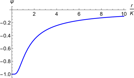
Figure 1: Sketch of the scalar field solution of Eq.(33), $\psi(r)=\phi(r)/\eta$ vs $r/K$, with $K\eta=1$.

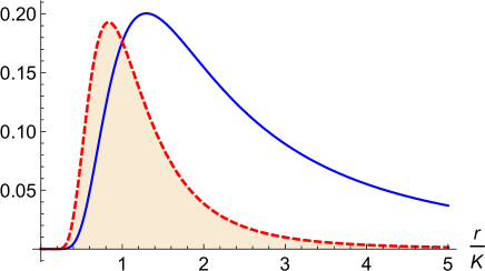
Figure 2: Sketches of the electric field, $QE_{r}(r)$ (solid) and the field energy density, $\mathcal{H}(r)$ (dashed, shaded)  of Eq.(33) vs $r/K$. ($K\eta$ has been set to $1$.)

For this model the BPS solution $\phi(r)$ is everywhere finite and asymptotes to zero at $r=\infty$. The energy density $\mathcal{H}(r)$ is localized, as typical for a solitonic configuration, and the electric field $E_{r}(r)$ deviates substantially from a pure $1/r^{2}$ behavior, instead, being pronounced with a maximum at a finite nonzero distance from the charge, and approaching zero near the charge. The total energy (mass) of the scalar field is

$$\mathcal{M}=4\pi\int_{0}^{\infty}\mathcal{H}(r)r^{2}dr=4\pi K^{2}\eta^{2}\int_{0}^{\infty}\frac{1}{r^{2}}\text{sech}^{4}\Big{(}\frac{K}{r}\Big{)}dr=8\pi K\eta^{2}\ .$$ (34)

From (33a) we have the asymptotic behavior $\phi(r)=-\eta\tanh(K/r)\sim-K\eta/r$, so that we can identify a scalar charge $Q_{s}=\pm K\eta$. (The $\pm$ sign is chosen since we could choose the $\pm$ sign for our $X(\phi)$ to get the same $\mathbf{E}$ and $\mathcal{H}$.)

V.1.2 Second model: $X(\phi)=\lambda(\eta^{2}-\phi^{2})^{1/2}$

This type of system was briefly looked at as an example of scalarization in the absence of gravity in Refs.Herdeiro PRL18 and Herdeiro PRD21 . In this case, by (30) and (31), $\varepsilon^{-1}(\phi)\sim X^{2}(\phi)\sim\lambda^{2}(\eta^{2}-\phi^{2})$ and $V_{E}(r,\phi)=\frac{1}{2r^{4}}\lambda^{2}(\eta^{2}-\phi^{2})$. The effective potential $V_{E}(r,\phi)\propto X^{2}(\phi)$ has no local minima in field space, but the effective scalar field mass parameter $m_{\phi}^{2}$ is negative, $\partial_{\phi}^{2}V_{E}(r,\phi)=-\lambda^{2}/r^{4}<0$, so that a tachyonic instability presents itself.

Again, by (30), (32), (31), and (20) we have a solution $\psi(r)=\phi(r)/\eta$, auxiliary function $X(r)$, electric field $E_{r}(r)$, and energy density $\mathcal{H}(r)$ (Fig.3),

$$\psi(r) =\sin\Big{(}\frac{\lambda}{r}\Big{)},$$ (35a)

$$X(r) =\lambda\eta\cos\Big{(}\frac{\lambda}{r}\Big{)},$$ (35b)

$$E_{r}(r) =\frac{1}{Q^{2}r^{2}}X^{2}(r)=\frac{\lambda^{2}\eta^{2}}{Q^{2}r^{2}}\cos^{2}\Big{(}\frac{\lambda}{r}\Big{)},$$ (35c)

$$\mathcal{H}(r) =2V_{E}(r)=\frac{1}{r^{4}}X^{2}(r)=\frac{\lambda^{2}\eta^{2}}{r^{4}}\cos^{2}\Big{(}\frac{\lambda}{r}\Big{)}.$$ (35d)

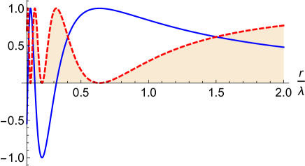
Figure 3: Sketch of the behavior of the scalar field solution of Eq.(35), $\psi(r)=\phi(r)/\eta$ (solid) and $X^{2}(r)$ (dashed, shaded) vs $r/\lambda$.  The electric field $E_{r}(r)$ and energy density $\mathcal{H}(r)$ vary rapidly with large amplitudes for small $r$.

This BPS solution is also localized (provided that the radius $r_{0}$ of the charge is nonzero), as are the electric field $E_{r}(r)$ and energy density $\mathcal{H}(r)$. Again it can be noted that the electric field is substantially different from a pure Coulombic case with a pure $1/r^{2}$ behavior. Instead, $E_{r}$ and $\mathcal{H}$ can oscillate at small distances from the charge, approaching zero as $r\rightarrow\infty$. The oscillatory behavior of $\mathcal{H}(r)$ can be associated with a sort of shell-like structure near the charge. The total energy (mass) of the scalar field is

$$\mathcal{M}(r_{0})=4\pi\int_{r_{0}}^{\infty}\mathcal{H}(r)r^{2}dr=4\pi\lambda^{2}\eta^{2}\int_{r_{0}}^{\infty}\frac{1}{r^{2}}\cos^{2}\Big{(}\frac{\lambda}{r}\Big{)}dr=\pi\lambda\eta^{2}\left[\sin\Big{(}\frac{2\lambda}{r_{0}}\Big{)}+\frac{2\lambda}{r_{0}}\right]\ ,$$ (36)

where $r_{0}$ is the radius of the charged object, serving as a short distance cutoff. From (35a), asymptotically $\phi\sim\lambda\eta/r$, allowing an identification of a scalar charge $Q_{s}=\pm\lambda\eta$.

V.2 Charged body in Reissner-Nordstrom background

The BPS ansatz for generating a first order Bogomolnyi equation for the Maxwell-scalar system in a fixed spacetime background can be extended to the case where an astrophysical object with mass $M$ and charge $Q_{0}=4\pi Q$ has a non-negligible effect upon the spacetime geometry. Here, we consider the case where the metric is the Reissner-Nordstrom metric:

$$ds^{2}=\left(1-\frac{r_{S}}{r}+\frac{r_{Q}^{2}}{r^{2}}\right)dt^{2}-\left(1-\frac{r_{S}}{r}+\frac{r_{Q}^{2}}{r^{2}}\right)^{-1}dr^{2}-r^{2}d\Omega^{2}$$ (37)

with $r_{S}=2GM$ and $r_{Q}^{2}=GQ_{0}^{2}/4\pi=4\pi GQ^{2}$. This can be rewritten in terms of geometrized mass and charge parameters $2\mu\equiv r_{S}$ and $q\equiv r_{Q}$, with $\mu$ and $q$ both having units of length. We then have

$$ds^{2}=\left(1-\frac{2\mu}{r}+\frac{q^{2}}{r^{2}}\right)dt^{2}-\left(1-\frac{2\mu}{r}+\frac{q^{2}}{r^{2}}\right)^{-1}dr^{2}-r^{2}d\Omega^{2}\ .$$ (38)

For this case we have

$$A(r)=\left(1-\frac{2\mu}{r}+\frac{q^{2}}{r^{2}}\right),\ \ \ B(r)=A^{-1}(r),\ \ \ h(r)=A(r),\ \ \ f(r)=r^{2}.$$ (39)

An important parameter to consider in this case is the ratio $\mu/q$ where $q$ is the magnitude of the charge, although here, for definiteness, we consider the charge to be positive. For $\mu>q$ there are two horizons located by $r_{\pm}=\mu\pm\sqrt{\mu^{2}-q^{2}},$ and for the extremal state $\mu=q$ the two coincide. However, for $\mu<q$ there are no horizons. This is the case that will be of interest here - the case $\mu/q<1$. The reason is that to find a real valued first order Bogomolnyi solution using the BPS ansatz of (17), the integral on the right hand side of (17a) must be real valued for all $r>0$:

$$\int\frac{dr}{f(r)h(r)}=\int\frac{dr}{\left(1-\frac{2\mu}{r}+\frac{q^{2}}{r^{2}}\right)r^{2}}=\frac{1}{\sqrt{q^{2}-\mu^{2}}}\tan^{-1}\left(\frac{r/q-\mu/q}{\sqrt{1-\mu^{2}/q^{2}}}\right)\ .$$ (40)

For $\mu/q>1$ this becomes complex valued, and therefore no real valued solution for all $r>\mu$ to the first order Bogomolnyi equation exists. We therefore consider the case $q>\mu$. The possibility that this condition may be physically realized for certain astrophysical objects has been considered (see, for example,Ray PRD03 ,Ray BJP04 ,Carvalho EPJC18 ).

V.2.1 First model: $X(\phi)=\lambda(\eta^{2}-\phi^{2})$

Now we again take $X(\phi)=\lambda(\eta^{2}-\phi^{2})$ as given in (32), or $X=K\eta(1-\psi^{2})$, with $\psi=\phi/\eta$ and $K=\lambda\eta$. Eqs. (17a) and (40) then yield the solution $\psi(r)$ (Fig.4),

$$\psi(r)=\tanh\left\{\frac{K/q}{\sqrt{1-\mu^{2}/q^{2}}}\Big{[}\tan^{-1}\Big{(}\frac{r/q-\mu/q}{\sqrt{1-\mu^{2}/q^{2}}}\Big{)}\Big{]}\right\}=\tanh\Theta(r),$$ (41)

where

$$\Theta(r)\equiv\frac{K/q}{\sqrt{1-\mu^{2}/q^{2}}}\Big{[}\tan^{-1}\Big{(}\frac{r/q-\mu/q}{\sqrt{1-\mu^{2}/q^{2}}}\Big{)}\Big{]}.$$ (42)

With (41), we obtain, with (14b), (16), and (25) (Fig.4),

$$X(r) =K\eta\left[1-\tanh^{2}\Theta(r)\right]=K\eta\ \text{sech}^{2}\Theta(r)\ ,$$ (43a)

$$\varepsilon^{-1}(r,\phi) =\frac{1}{AQ^{2}}X^{2}(\phi)=\frac{K^{2}\eta^{2}\ \text{sech}^{4}\Theta(r)}{Q^{2}(1-\frac{2\mu}{r}+\frac{q^{2}}{r^{2}})}\ ,$$ (43b)

$$E_{r} =\frac{Q}{\varepsilon r^{2}}=\frac{1}{QAr^{2}}X^{2}=\frac{K^{2}\eta^{2}\ \text{sech}^{4}\Theta(r)}{Qr^{2}(1-\frac{2\mu}{r}+\frac{q^{2}}{r^{2}})}\ ,$$ (43c)

$$\mathcal{H} =T_{0}^{0}=2V_{E}=\frac{1}{f^{2}h}X^{2}(\phi)=\frac{K^{2}\eta^{2}\ \text{sech}^{4}\Theta(r)}{r^{4}(1-\frac{2\mu}{r}+\frac{q^{2}}{r^{2}})}\ .$$ (43d)

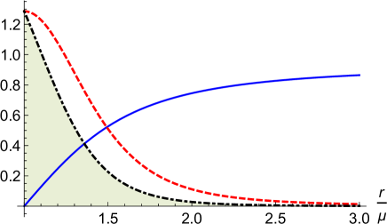
Figure 4: Sketches of the solution $\psi(r)$ (solid) of Eq.(41), electric field, $QE_{r}(r)$ (dashed) and the field energy density, $\mathcal{H}(r)$ (dot-dashed, shaded)  of Eq.(43) vs $r/\mu$. Here we use the settings $\mu/q=K/q=3/4$, and $K\eta$ has been set to $1$.

The solution for $\phi(r)$ is finite, and approaches a constant value of $\phi(\infty)=\eta\tanh\Theta(\infty)=\eta\tanh[\frac{\pi K/q}{2\sqrt{1-\mu^{2}/q^{2}}}]$. Again, the behaviors of $E_{r}(r)$ and $\mathcal{H}(r)$ differ from the Coulombic case, due to the factor of $A^{-1}(r)$sech${}^{4}\Theta(r)$.

To get an expression for a scalar charge, we look at the asymptotic behavior of (41). First, we write (41) as

$$\psi(r)=\tanh[A\tan^{-1}(x)];\ \ \ A=\frac{K/q}{\sqrt{1-q^{2}/\mu^{2}}},\ \ \ x=\Big{(}\frac{r/q-\mu/q}{\sqrt{1-\mu^{2}/q^{2}}}\Big{)},$$ (44)

and

$$\tanh[A\tan^{-1}(x)]\sim\tanh[A(\pi/2-1/x)]\sim\tanh(\frac{\pi A}{2})-\frac{A\text{sech}^{2}(\frac{\pi A}{2})}{x}\ .$$ (45)

As $r\rightarrow\infty$,

$$\frac{1}{x}=\sqrt{1-\mu^{2}/q^{2}}(\frac{r}{q}-\frac{\mu}{q})^{-1}\sim\frac{q\sqrt{1-\mu^{2}/q^{2}}}{r}\ .$$ (46)

We then have $\phi(r)\sim\phi_{0}+Q_{s}/r$ as $r\rightarrow\infty$, where $\phi_{0}=\phi(\infty)=\tanh(\frac{\pi A}{2})$. Then $\phi(r)\sim\phi_{0}-A$sech${}^{2}(\frac{\pi A}{2})\cdot\frac{q\sqrt{1-\mu^{2}/q^{2}}}{r}$. A scalar charge is then identified;

$$Q_{s}=\pm\eta A\text{sech}^{2}(\frac{\pi A}{2})\cdot q\sqrt{1-\mu^{2}/q^{2}}=\pm K\eta\ \text{sech}^{2}(\frac{\pi A}{2})\ .$$ (47)

V.2.2 Second model: $X(\phi)=\lambda(\eta^{2}-\phi^{2})^{1/2}$

For this model we have the same integral given by (40) and (17a) gives

$$\int\frac{d\phi}{X(\phi)}=\int\frac{d\phi}{\lambda(\eta^{2}-\phi^{2})^{1/2}}=\int\frac{d\psi}{\lambda(1-\psi^{2})^{1/2}}=\frac{1}{\lambda}\sin^{-1}\psi,$$ (48)

where $\psi=\phi/\eta$. Therefore, by (48) and (40),

$$\psi(r)=\sin\left\{\frac{\lambda}{\sqrt{q^{2}-\mu^{2}}}\tan^{-1}\left(\frac{r/q-\mu/q}{\sqrt{1-\mu^{2}/q^{2}}}\right)\right\}=\sin\Phi(r),$$ (49)

where

$$\Phi(r)\equiv\frac{\lambda}{\sqrt{q^{2}-\mu^{2}}}\tan^{-1}\left(\frac{r/q-\mu/q}{\sqrt{1-\mu^{2}/q^{2}}}\right)\ .$$ (50)

With (49) and with (14b), (16), and (25) we have (Fig.5)

$$X(r) =\lambda\eta(1-\psi^{2})^{1/2}=\lambda\eta\cos\Phi(r)\ ,$$ (51a)

$$\varepsilon^{-1}(r,\phi) =\frac{1}{AQ^{2}}X^{2}(\phi)=\frac{\lambda^{2}\eta^{2}\cos^{2}\Phi(r)}{Q^{2}(1-\frac{2\mu}{r}+\frac{q^{2}}{r^{2}})}\ ,$$ (51b)

$$E_{r} =\frac{Q}{\varepsilon r^{2}}=\frac{1}{QAr^{2}}X^{2}=\frac{\lambda^{2}\eta^{2}\cos^{2}\Phi(r)}{Qr^{2}(1-\frac{2\mu}{r}+\frac{q^{2}}{r^{2}})}\ ,$$ (51c)

$$\mathcal{H} =T_{0}^{0}=2V_{E}=\frac{1}{f^{2}h}X^{2}(\phi)=\frac{\lambda^{2}\eta^{2}\cos^{2}\Phi(r)}{r^{4}(1-\frac{2\mu}{r}+\frac{q^{2}}{r^{2}})}\ .$$ (51d)

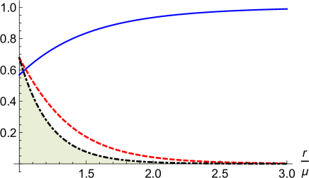
Figure 5: Sketches of the solution $\psi(r)$ (solid) of Eq.(49), electric field, $QE_{r}(r)$ (dashed) and the field energy density, $\mathcal{H}(r)$ (dot-dashed, shaded)  of Eq.(51) vs $r/\mu$. Here we use the settings $\mu/q=1/2$, and $\lambda/q$ has been set to $1$.

The solution for $\phi(r)$ is finite, and approaches a constant value of $\phi(\infty)=\eta\sin[\frac{\pi\lambda}{2\sqrt{q^{2}-\mu^{2}}}]$. Again, the behaviors of $E_{r}(r)$ and $\mathcal{H}(r)$ differ from the Coulombic case, due to the factor of $A^{-1}(r)$cos${}^{2}\Phi(r)$.

To find a scalar charge, write (49) as

$$\psi(r)=\sin[C\tan^{-1}(x)];\ \ \ C=\frac{\lambda/q}{\sqrt{1-\mu^{2}/q^{2}}},\ \ \ x=\Big{(}\frac{r/q-\mu/q}{\sqrt{1-\mu^{2}/q^{2}}}\Big{)}\ .$$ (52)

As $r\rightarrow\infty$,

$$\psi(r)\sim\sin[C(\frac{\pi}{2}-\frac{1}{x})]\sim\sin(\frac{\pi C}{2})-\frac{C\cos(\frac{\pi C}{2})}{x}\sim\sin(\frac{\pi C}{2})-\frac{Cq\sqrt{1-q^{2}/\mu^{2}}}{r}\cos(\frac{\pi C}{2})\ .$$ (53)

Then $\phi(r)=\eta\psi(r)$ with $\phi\sim\phi_{0}-Q_{s}/r$, where $\phi_{0}=\eta\sin(\frac{\pi C}{2})$ and

$$Q_{s}=\pm\eta Cq\sqrt{1-q^{2}/\mu^{2}}\cos(\frac{\pi C}{2})=\pm\lambda\eta\cos(\frac{\pi C}{2})\ .$$ (54)

To briefly summarize, we note that real-valued first order Bogomolnyi solutions (for all $r>0$) are not available for the Reissner-Nordstrom metric here for geometrized parameters $q\leq\mu$ (in which case there are horizons), which excludes such scalarized BPS ansatz solutions for undercharged or extremal Reissner-Nordstrom black holes. Solutions to the second order equations of motion can exist, though. However, real-valued first order Bogomolnyi solutions are available for compact objects for which $q>\mu$ (in which case there are no horizons). One possibility for such a compact object is an overcharged neutron star or white dwarf Ray PRD03 ,Ray BJP04 ,Carvalho EPJC18 , or an object that has collapsed to a naked singularity before losing all of its charge Ray PRD03 .

VI Discussion

The possibility of a scalar field being found concentrated around a gravitating object, such as a black hole, has been investigated extensively since the emergence of the idea in the context of scalar-tensor theory Damour PRL93 ,Damour PRD96 . (See the review by Herdeiro and Radu Herdeiro IJMPD15 , and references therein.) In addition, there have been investigations into the possibility of scalarizing solutions around electrically charged sources (see Refs.Cvetic NPB94 ,BBFR 03 -Issifu AHEP21 ,Herdeiro EPJC20 ,Bazeia EPJC21 , and Herdeiro PRL18 -Garcia 21 for example.) By adopting a fixed background metric, some of the complications due to gravitation can be evaded while capturing essential qualitative features Bazeia EPJC21 , Herdeiro PRL18 , Herdeiro PRD21 of the scalar field.

The idea of scalarization within the context of Maxwell-scalar theory has been considered here, where the “on-shell method” of Atmaja and Ramadhan Atmaja PRD14 has been used to obtain exact, analytic closed-form solutions to first order Bogomolnyi equations, along with a constraint on the form of the effective potential. The first order Bogomolnyi equation can then be solved by quadrature. These minimal energy BPS solutions automatically satisfy the second order Euler-Lagrange equations of motion, and are radially stable, i.e., stable against spontaneous radial expansion or collapse JM PRD21 ,Mandal EPL21 . A nonlinear coupling function, or “effective permittivity” $\varepsilon(r,\phi)$, may allow a tachyonic instability, which then gives rise to a scalar cloud, in the form of a nontopological soliton, around an electrically charged source.

Here, two examples of BPS solutions for a real scalar field $\phi(r)$ responding to an electrically charged source have been presented with two forms of an effective scalar-Maxwell coupling function $\varepsilon(r,\phi)$, generated by the auxiliary functions $X(\phi)$. These two forms for $\varepsilon$ have been looked at previously in the context of a flat Minkowski background Bazeia EPJC21 ,Herdeiro PRL18 ,Herdeiro PRD21 , where gravitation plays no part. These solutions for a Minkowski background have been recovered here, and then extended to the case of a Reissner-Nordstrom background, where both gravitation and electromagnetism are present, and are not ignored. Exact, closed form, analytical solutions have been found for each situation. These solutions provide descriptions for the profiles of the scalar field $\phi(r)$, the electric field $E_{r}(r)$, and the scalar field energy density $\mathcal{H}(r)=T_{0}^{0}(r)$.

The situations for a point charge or charged sphere in Minkowski spacetime, were briefly reviewed, and the basic results found in Refs.Bazeia EPJC21 and Herdeiro PRL18 were recovered. Next, using similar coupling functions, a nonrotating charged compact object with an exterior Reissner-Nordstrom background was considered. Specifically, an overcharged object with a geometrized charge to mass ratio $q/\mu>1$ was seen to provide an example of scalarization that could be relevant to highly charged neutron stars Ray PRD03 ,Ray BJP04 or white dwarfs Carvalho EPJC18 .

In these examples closed form analytical solutions have been obtained to describe the scalar cloud and attendant electric field $\mathbf{E}(r)$. The examples for a Minkowski background have recovered the solutions previously presented in Refs.Bazeia EPJC21 and Herdeiro PRL18 , and the solutions for the Reissner-Nordstrom background are, to our knowledge, new. The effective permittivity $\varepsilon(r,\phi)$ gives rise to electric fields $\mathbf{E}(r)$ which deviate substantially from the Coulombic ones that would be expected from pure Maxwell theory with $\varepsilon=1$ and no scalar coupling. If a gravitating source is electrically charged, and the electric field is modified from its Coulombic form, then there may be observable effects on a surrounding medium. For instance, radiation emitted by an accelerated charged particle in a such an altered electric field would differ from that of a charged particle in a Coulombic electric field of an unscalarized charged source. Consequently, it may be possible to infer the presence of scalar fields near charged, gravitating bodies. The features exhibited by exact, closed form BPS solutions are expected to also be seen, at least in a qualitative way, in non-BPS solutions where scalar back reactions are accounted for, or for a case where a coupling function $\varepsilon(\phi)$ is not of the BPS form. In addition, it could be of interest to see what the effects of a scalar mass or an additional scalar potential $V(\phi)$ may be.

References

- (1) M. Cvetic and A.A. Tseytlin, “Charged string solutions with dilaton and modulus fields”, Nucl. Phys. B 416 (1994) 137-172 • e-Print: hep-th/9307123 [hep-th]
- (2) D. Bazeia, F.A. Brito, W. Freire, R.F. Ribeiro, “Confining potential in a color dielectric medium with parallel domain walls”, Int. J. Mod. Phys. A 18 (2003) 5627-5636 • e-Print: hep-th/0210289 [hep-th]
- (3) D. Bazeia, F.A. Brito, W. Freire, R.F. Ribeiro, “Confinement from new global defect structures”, Eur. Phys. J. C 40 (2005) 531-537 • e-Print: hep-th/0311160 [hep-th]
- (4) F.A. Brito, M.L.F. Freire, W. Serafim, “Confinement and screening in tachyonic matter”, Eur. Phys. J. C 74 (2014) 12, 3202 • e-Print: 1411.5656 [hep-th]
- (5) A. Issifu, F.A. Brito, “An Effective Model for Glueballs and Dual Superconductivity at Finite Temperature”, Adv. High Energy Phys. 2021 (2021) 5658568 • e-Print: 2105.01013 [hep-ph]
- (6) C.A.R. Herdeiro, J.M.S. Oliveira, and E. Radu, “A class of solitons in Maxwell-scalar and Einstein–Maxwell-scalar models”, Eur. Phys. J. C 80 (2020) 1, 23 • e-Print: 1910.11021 [gr-qc]
- (7) D. Bazeia, M.A. Marques, R. Menezes, “Electrically charged localized structures”, Eur. Phys. J. C 81 (2021) 1, 94 • e-Print: 2011.01766 [physics.gen-ph]
- (8) E. B. Bogomolny, “Stability of Classical Solutions”, Yad. Fiz. 24 (1976) 861 [Sov. J. Nucl. Phys. 24 (1976) 449
- (9) M. K. Prasad and C. M. Sommerfield, “Exact Classical Solution for the ’t Hooft Monopole and the Julia-Zee Dyon”, Phys. Rev. Lett. 35 (1975) 760
- (10) A. N. Atmaja, H. S. Ramadhan, “Bogomol’nyi equations of classical solutions”, Phys. Rev. D 90 (2014) 10, 105009 • e-Print: 1406.6180 [hep-th]
- (11) T. Damour, G. Esposito-Farese, “Nonperturbative strong field effects in tensor - scalar theories of gravitation”, Phys. Rev. Lett. 70 (1993) 2220-2223
- (12) T. Damour, G. Esposito-Farese, “Tensor - scalar gravity and binary pulsar experiments”, Phys. Rev. D 54 (1996) 1474-1491 • e-Print: gr-qc/9602056 [gr-qc]
- (13) C.A.R. Herdeiro, E. Radu, “Asymptotically flat black holes with scalar hair: a review”, Int. J. Mod. Phys. D 24 (2015) 09, 1542014 • Contribution to: 7th Black Holes Workshop 2014 • e-Print: 1504.08209 [gr-qc]
- (14) C.A.R. Herdeiro, E. Radu, N. Sanchis-Gual, J.A. Font, “Spontaneous Scalarization of Charged Black Holes”, Phys. Rev. Lett. 121 (2018) 10, 101102 • e-Print: 1806.05190 [gr-qc]
- (15) C.A.R. Herdeiro, T. Ikeda, M. Minamitsuji, T. Nakamura, E. Radu, “Spontaneous scalarization of a conducting sphere in Maxwell-scalar models”, Phys. Rev. D 103 (2021) 4, 044019 • e-Print: 2009.06971 [gr-qc]
- (16) Y.S. Myung, De-Cheng Zou, “Quasinormal modes of scalarized black holes in the Einstein–Maxwell–Scalar theory”, Phys. Lett. B 790 (2019) 400-407 • e-Print: 1812.03604 [gr-qc]
- (17) P.G.S. Fernandes, C.A.R. Herdeiro, A.M. Pombo, E. Radu, N. Sanchis-Gual, “Spontaneous Scalarisation of Charged Black Holes: Coupling Dependence and Dynamical Features”, Class. Quant. Grav. 36 (2019) 13, 134002, Class.Quant.Grav. 37 (2020) 4, 049501 (erratum) • e-Print: 1902.05079 [gr-qc]
- (18) P.G.S. Fernandes, C.A.R. Herdeiro, A.M. Pombo, E. Radu, N. Sanchis-Gual, “Charged black holes with axionic-type couplings: Classes of solutions and dynamical scalarization”, Phys. Rev. D 100 (2019) 8, 084045 • e-Print: 1908.00037 [gr-qc]
- (19) De-Cheng Zou, Y.S. Myung,“ Scalarized charged black holes with scalar mass term”, Phys. Rev. D 100 (2019) 12, 124055 • e-Print: 1909.11859 [gr-qc]
- (20) Y. Brihaye, B. Hartmann, “Spontaneous scalarization of charged black holes at the approach to extremality”, Phys. Lett. B 792 (2019) 244-250 • e-Print: 1902.05760 [gr-qc]
- (21) T. Ikeda, T. Nakamura, M. Minamitsuji,“Spontaneous scalarization of charged black holes in the Scalar-Vector-Tensor theory”, Phys. Rev. D 100 (2019) 10, 104014 • e-Print: 1908.09394 [gr-qc]
- (22) P.G.S. Fernandes, “Einstein–Maxwell-scalar black holes with massive and self-interacting scalar hair”, Phys. Dark Univ. 30 (2020) 100716 • e-Print: 2003.01045 [gr-qc]
- (23) S. Hod, “Spontaneous scalarization of charged Reissner-Nordström black holes: Analytic treatment along the existence line”, Phys. Lett. B 798 (2019) 135025 • e-Print: 2002.01948 [gr-qc]
- (24) S. Hod, “Reissner-Nordström black holes supporting nonminimally coupled massive scalar field configurations”, Phys. Rev. D 101 (2020) 10, 104025 • e-Print: 2005.10268 [gr-qc]
- (25) D.D. Doneva, S. Kiorpelidi, P.G. Nedkova, E. Papantonopoulos, S.S. Yazadjiev, “Charged Gauss-Bonnet black holes with curvature induced scalarization in the extended scalar-tensor theories”, Phys. Rev. D 98 (2018) 10, 104056 • e-Print: 1809.00844 [gr-qc]
- (26) G. García, M. Salgado, “Regular scalar charged clouds around a Reissner-Nordstrom black hole and no-hair theorems”, Phys. Rev. D 104 (2021) 6, 064054 • e-Print: 2107.06933 [gr-qc]
- (27) T. P. Sotiriou,” Black Holes and Scalar Fields”, Class. Quant. Grav. 32 (2015) 21, 214002 • e-Print: 1505.00248 [gr-qc]
- (28) J.R. Morris, “Radially symmetric scalar solitons”, Phys. Rev. D 104 (2021) 1, 016013 • e-Print: 2107.02861 [hep-th]
- (29) S. Mandal, “Solitons in curved spacetime”, EPL (2021) (in press)
- (30) S. Ray, A.L. Espindola, M. Malheiro, J.P.S. Lemos, V.T. Zanchin, “Electrically charged compact stars and formation of charged black holes”, Phys. Rev. D 68 (2003) 084004 • e-Print: astro-ph/0307262 [astro-ph]
- (31) S. Ray, M. Malheiro, J.P.S. Lemos, V.T. Zanchin, “Charged polytropic compact stars”, Braz. J. Phys. 34 (2004) 310-314 • e-Print: nucl-th/0403056 [nucl-th]
- (32) G.A. Carvalho, J.D.V. Arbañil, R.M. Marinho, M. Malheiro, “White dwarfs with a surface electrical charge distribution: Equilibrium and stability”, Eur. Phys. J. C 78 (2018) 5, 411 • e-Print: 1805.07257 [astro-ph.SR]
- (33) G. Panotopoulos, T. Tangphati, A. Banerjee, “Electrically charged compact stars with an interacting quark equation of state”, e-Print: 2105.10638 [gr-qc]
- (34) For notational convenience (to avoid writing explicit factors of ), we use a rationalized charge , where is the total charge associated with an ordinary Gauss’ law and electric field in Minkowski space, with. The free space permittivity is , and in natural units (), . We have for the Reissner-Nordstrom metric.
- (35) D. Bazeia, J. Menezes, R. Menezes, “New global defect structures”, Phys. Rev. Lett. 91 (2003) 241601 • e-Print: hep-th/0305234 [hep-th]
- (36) G.H. Derrick, “Comments on nonlinear wave equations as models for elementary particles”, J. Math. Phys. 5 (1964) 1252-1254