Scaling, mirror symmetries and consonances among the distances of the planets of the solar system

Abstract

Orbital systems are often self-organized and/or characterized by harmonic relations. Inspired by music theory, we rewrite the Geddes and King-Hele (QJRAS, 24, 10–13, 1983) equations for mirror symmetries among the distances of the planets of the solar system in an elegant and compact form by using the 2/3rd power of the ratios of the semi-major axis lengths of two neighboring planets (eight pairs, including the belt of the asteroids). This metric suggests that the solar system could be characterized by a scaling and mirror-like structure relative to the asteroid belt that relates together the terrestrial and Jovian planets. These relations are based on a 9/8 ratio multiplied by powers of 2, which correspond musically to the interval of the Pythagorean epogdoon (a Major Second) and its addition with one or more octaves. Extensions of the same model are discussed and found compatible also with the still hypothetical vulcanoid asteroids versus the transneptunian objects. The found relation also suggests that the planetary self-organization of our system could be generated by the 3:1 and 7:3 resonances of Jupiter, which are already known to have shaped the asteroid belt. The proposed model predicts the main Kirkwood asteroid gaps and the ratio among the planetary orbital parameters with a 99% accuracy, which is three times better than an alternative, recently proposed harmonic-resonance model for the solar system. Furthermore, the ratios of neighboring planetary pairs correspond to four musical “consonances” having frequency ratios of 5/4 (Major Third), 4/3 (Perfect Fourth), 3/2 (Perfect Fifth) and 8/5 (Minor Sixth); the probability of obtaining this result randomly has a $p<0.001$. Musical consonances are “pleasing” tones that harmoniously interrelate when sounded together, which suggests that the orbits of the planets of our solar system could form some kind of gravitationally optimized and coordinated structure. Physical modeling indicates that energy non-conserving perturbations could drive a planetary system into a self-organized periodic state with characteristics vaguely similar of those found in our solar system. However, our specific finding suggests that the planetary organization of our solar system could be rather peculiar and based on more complex and unknown dynamical structures.

¹Danbury Music Centre, Danbury, CT, 06810 USA..

²Department of Earth Sciences, Environment and Georesources, University of Naples Federico II, Complesso Universitario di Monte S. Angelo, via Cinthia, 21, 80126 Naples, Italy.

^†These authors share first authorship.

^*Corresponding author: nicola.scafetta@unina.it

Keywords: Solar system; orbital self-organization; mirror symmetries; orbital resonances; music and astronomy.

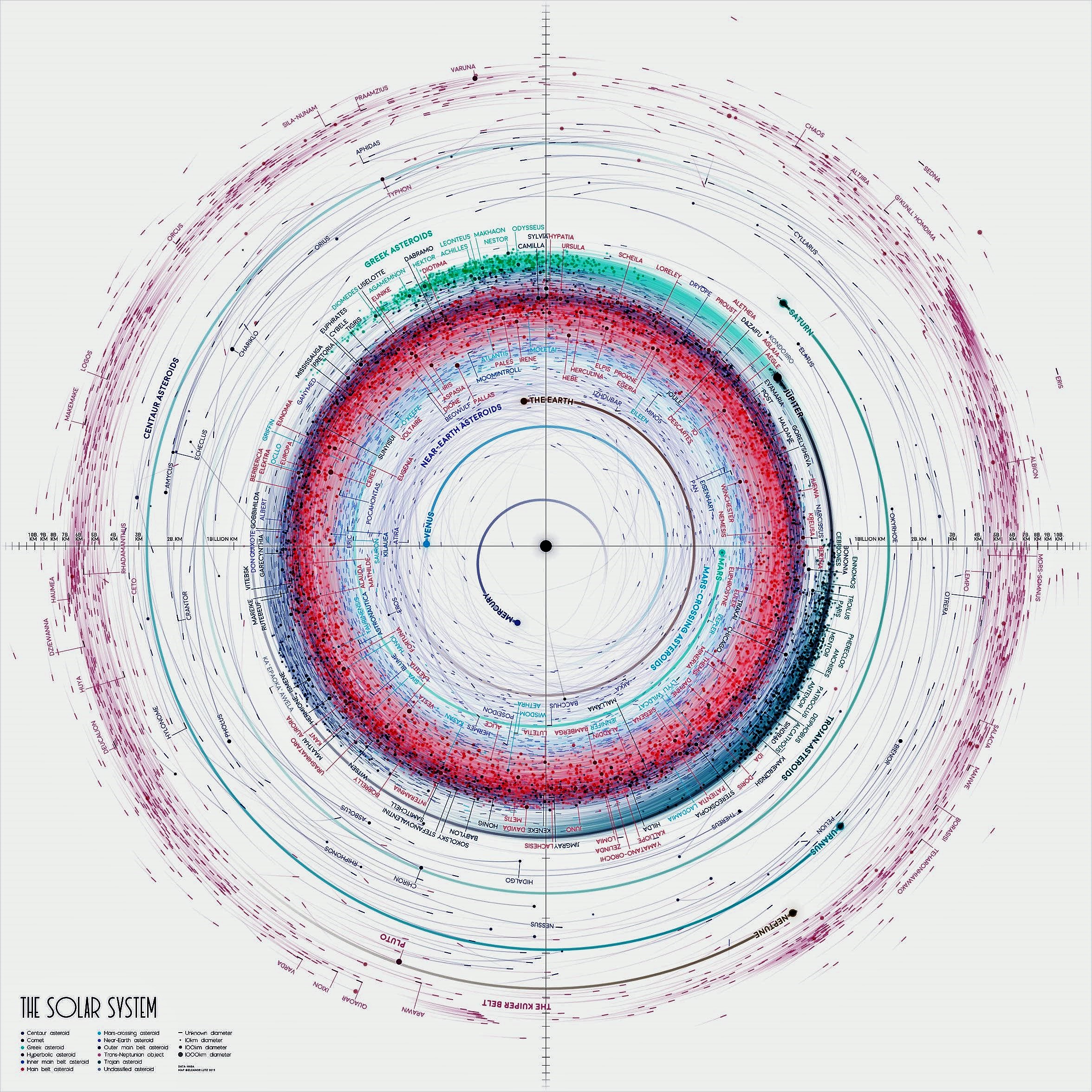
Figure 8: A nice presentation of the solar system. This map shows in a logarithmic scale the orbit paths of the planets of the solar system together with those of about 18,000 asteroids and comets larger than 10 km in diameter. Adapted from Lutz (2019, CC BY-NC-ND 4.0).

Note: The present copy slightly updates the published paper with the addition of Table 7 and relative comment on pages 15 and 16, with the artwork of the solar system depicted in Figure 8 (page 19) and the Appendix on page 20.

1 Introduction

Since ancient times the stability of the solar system, its regularities, and the movements of its planets have attracted the attention of astronomers and philosophers because their orbital revolutions appeared to be related by simple proportions (Haar, 1948; Stephenson, 1974; Godwin, 1992). This observation yielded the understanding that solar and lunar systems could be characterized by harmonic resonances, which are usually the result of self-organizing gravitational or tidal processes yielding to long-term stable planet and moon orbits (Aschwanden, 2018; Moons and Morbidelli, 1995). In fact, planetary circular orbits are dynamically unstable, unless their mutual orbital periods fall into harmonic whole number ratios called “orbital commensurabilities” (McFadden et al., 1999; Peale, 1976; Pakter and Levin, 2018).

For example, within our solar system, 5 orbital periods of Jupiter approximately correspond to 2 periods of Saturn, 13 orbital periods of Venus approximately correspond to 8 periods of the Earth, and Pluto makes two orbits for every three of Neptune (cf: Scafetta, 2014a). In addition, there are the well-known 1:2:4 resonances of Jupiter’s moons Ganymede, Europa and Io, which was studied by Pierre-Simon Laplace (1749 – 1827), and the primary gaps in the asteroid main-belt at the 4:1, 3:1, 5:2, 7:3, 2:1 mean-motion resonances between the asteroids and Jupiter, which was first noticed in 1866 by Daniel Kirkwood (1814 – 1895) (Moons and Morbidelli, 1995; Moons et al., 1998).

The Trappist-1 solar system is also a very peculiar exoplanetary example. It is made of a dwarf red star and seven earth-size planets labeled b, c, d, e, f, g, and h (three are in the habitable zone) whose stable orbits are characterized by three-body Laplace-type near-resonances (Gillon et al., 2017; Luger et al., 2017; Tamayo et al., 2017). The seven orbital periods are: 1.511, 2.422, 4.049, 6.101, 9.207, 12.352, and 18.773 days, respectively (Agol et al., 2021). Thus, the period ratios between adjacent planet pairs (c/b, d/c, e/d, f/e, g/f and h/g) are 1.603, 1.672, 1.507, 1.509, 1.342, 1.520, respectively. These ratios are very close to the following integer ratios: 8:5, 5:3, 3:2, 3:2, 4:3, 3:2, respectively, with a mean relative error of 0.6%, which is the longest known series of near-resonant exoplanets. The planetary resonances of the Trappist-1 system’s motion are so accurate and peculiar that they were translated into music (Chang, 2017; Russo, 2018).

On a wider perspective, gravitational self-organization and harmonic resonances, and more specifically the planetary invariant inequalities involving planetary conjunctions and their beats, generate complex planetary synchronization structures in the solar system that appear to modulate also solar variability and climate change on Earth. These phenomena are currently under study by several authors (e.g.: Beer et al., 2018; Charvatova, 1997; Scafetta, 2014b; Scafetta et al., 2016; Scafetta, 2020; Stefani et al., 2021; Tattersall, 2013, and others).

The philosophical concept of orbital resonance is known as “Musica Universalis” or “Music of the Spheres” or “Harmony of the Spheres”, and was first developed in the 6th century BC by Pythagoras of Samos (570–495 BC) and his followers (Stephenson, 1974; Godwin, 1992; Rogers, 2016), who related planetary periods with the principles of musical harmony. The philosopher noted that the pitch of a musical note is in inverse proportion to the length of the string that produces it, and that intervals between harmonious sound frequencies form simple numerical ratios. Furthermore, Pythagoras proposed that the bodies of the solar system (including the Sun, the Moon and the planets) all emit a unique hum based on their orbital revolution. According to Philolaus (470 – 385 BC), the planetary harmonics were characterized by four basic musical intervals: 2:1 (octave), 3:2 (fifth), 4:3 (fourth) and 1:1 (unison).

Herein we adopt a similar transdisciplinary approach and show that music theory can still be useful to explore some possible unknown features that characterize the interplanetary gravitational organization of our solar system. Indeed, Kepler himself was inspired by musical principles (Cartwright et al., 2021).

In fact, the correspondence between whole number ratios in orbital resonances and music theory was further developed by Johannes Kepler (1571 – 1630) in Harmonices Mundi (The Harmony of the World, 1619), in which he related musical tones with the periods, distances and angular velocities of the planets (cf. Rogers, 2016). Very likely, Kepler’s conception of the “Music of the Worlds” reflected the polyphony of his day as developed by composers such as Giovanni Pierluigi da Palestrina (1525 – 1594).

For example, he noted that, relative to the Sun, the angular speed of the Earth varies by a semitone (a ratio of 16:15), between aphelion and perihelion. Similar musical relations were found for the other planets as well so that Kepler hypothesized the existence of a celestial choir made up of a tenor (Mars), two basses (Saturn and Jupiter), a soprano (Mercury), and two altos (Venus and Earth). These inquiries brought forth his discovery of the “third law of planetary motion”. We recall that Kepler’s first and second law of planetary motions were proposed 10 years earlier in Astronomia Nova (1609). Kepler’s laws were empirically based and published almost 100 years before Newton proposed the gravitational law that provided their physical basis.

The third law establishes that the square of a planet’s orbital period $T$ is proportional to the cube of the length of the semi-major axis of its orbit $a$ as:

$$a^{3}=cT^{2}=\frac{G(M_{\odot}+m)}{4\pi^{2}}T^{2}\approx\frac{GM_{\odot}}{4\pi^{2}}T^{2},$$ (1)

where $G$ is the universal gravitational constant, $m$ is the mass of the planet and $M_{\odot}$ is the mass of the Sun. Since $M_{\odot}$ is much larger than any planetary mass, $c$ can be considered constant for the entire solar system. Furthermore, $c=1$ if the period is measured in years and the semi-major axis length is measured in astronomical units (that is the mean distance between the Sun and the Earth). Finally, by establishing a simple relation between the period and the semi-major axis of an orbit ($a=T^{2/3}$ or $T=a^{3/2}$), Eq. 1 allows the rewriting of any planetary equation depending on one of these orbital parameters as a function of the other.

Further attempts to model the solar system using simple relations included the “Titius–Bode law of Planetary Distances” (Bode, 1772; Titius, 1766) that, with a good approximation, correctly reproduced the orbital position of Mercury, Venus, Earth, Mars, Jupiter and Saturn, and successfully predicted those of Ceres and Uranus, although it failed for Neptune. Additional attempts to improve such methods were proposed by other authors (e.g.: Basano and Hughes, 1979; Louise, 1982; Molchanov, 1968; Nieto, 1972), up to very recent times (e.g.: Tattersall, 2013; Scafetta, 2014a; Aschwanden, 2018, and cited references).

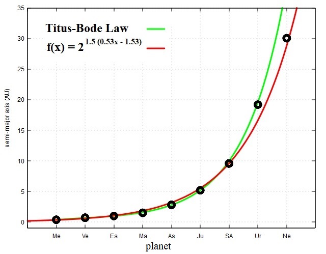
Figure 1: The semi-major axes of the planets versus the Titus-Bode law and a simple exponential fit.

Figure 1 shows the semi-major axes of the planets versus the Titus-Bode empirical law — $a_{z}=0.4+0.3\times 2^{z}$ for $z=-\infty$ (Mercury), 0 (Venus), 1 (Earth), 2 (Mars), … , 7 (Neptune) (Bode, 1772; Titius, 1766) — and a simple exponential fit of the type $f(x)=2^{(ax+b)\times 3/2}$, where the integer values of x denote the planet series number from 1 to 9. The fit gives $a=0.529\pm 0.016$ and $b=-1.53\pm 0.09$. These coefficients are very close to the whole-ratio 1/2 and -3/2, which might suggest an ideal equation of the type $a_{n}=2^{-9/4}2^{3n/4}\approx 0.21\times 1.68^{n}$, where $n$ goes from 1 (Mercury) to 9 (Neptune), and $n=5$ denotes the asteroid belt.

Similar relations are found in the theoretical literature. For example, Pakter and Levin (2018) studied the stability and self-organization of planetary systems similar to our solar system. Gravitational instabilities usually lead to catastrophic events because planets either collide or are ejected from the planetary system. However, these authors showed that if the planetary motion is quasi-periodic and the planets could gain or lose energy from interplanetary orbiting dust, then, computer simulations over astronomical time scales suggest that such systems could reach a planetary self-organized structure. The proposed equations were the following:

$$m\ddot{x}_{i}=-\frac{GMmx_{i}}{r_{i}^{3}}-\sum_{j}\frac{Gm^{2}(x_{i}-x_{j})}{r_{ij}}-f_{i}^{\theta}\frac{y_{i}}{r_{i}}$$ (2)

$$m\ddot{y}_{i}=-\frac{GMmy_{i}}{r_{i}^{3}}-\sum_{j}\frac{Gm^{2}(y_{i}-y_{j})}{r_{ij}}-f_{i}^{\theta}\frac{x_{i}}{r_{i}}$$ (3)

where $M$ is the sun’s mass, $m$ is the planet mass (which this model supposes to all be equal), $r_{i}$ is the distance between the sun and the planet $i$, $r_{ij}$ is the distance between the planets $i$ and $j$, and $f_{i}^{\theta}$ is the angular force responsible for the interaction between the planet $i$ and the residual dust of the protoplanetary disk.

Pakter and Levin (2018) demonstrated that systems up to 9 planets reach a self-organized dynamical state where the anomalistic periods between the radially adjacent planets could be synchronized in a near 2:1 resonance. Moreover, several simulations showed that the ratio of semi-major axis could follow a geometric progression of the type $r_{n}\sim c^{n}$, where $c$ is close to 1.6-1.7, which is similar to what was found for the solar system: see Figure 1. For example, for a perfect 2:1 resonance ratio, the semi-major axis lengths would follow a Titus-Bode-like relation of the type: $r_{n}\sim 2^{2n/3}\approx 1.59^{n}$. However, these authors were not able to find a stable planetary system made of more than 6 planets. They also acknowledged that the proposed mechanism could not be “unique” in explaining the self-organization of a solar system. In fact, they did not succeed in exactly simulating our solar system, which is made of 8 planets of different masses plus the Asteroid and Kuiper belts.

We also observe that a major problem with the Titius–Bode law (and also with the above fit function) is that such an equation is physically unconstrained because the parameter z (or n in the fitting function) do not have an upper theoretical limit, which implies that the equations would eventually fail the prediction. Also using $z=-\infty$ for Mercury in the original Titius–Bode law was arbitrary because such a value was chosen just to fix the divergence. Therefore, such equations do not appear to be statistically nor physically robust. In the following, we propose a mirror-like planetary model that does not suffer the same problem because it appears to be physically constrained by the properties of the solar system itself.

In this work, we first extend some of the calculations by Kepler (1619) to all eight planets of the solar system (in the 17th century the asteroid belt, Uranus and Neptune were unknown) and, in most cases, we found that simple whole-number ratios emerge in the periods, distances and angular velocities only for some planet pairs. This result, however, implies that a correspondent musical ratio can not be found for all planetary ratios, which suggests that our solar system is not characterized by a self-organization structure similar to that found, for example, in the Trappist-1 solar system. Thus, we searched alternative orbital metrics and checked whether they could produce a musical correspondence for all planetary pairs. The assumption is that ratios adopted in the traditional musical tuning systems and, in particular, those that form consonances, are peculiar because they are harmoniously interrelated and, therefore, may unearth important physical relations (Cartwright et al., 2021).

An interesting feature of the solar system is that it is made of four inner terrestrial planets (Mercury, Venus, Earth and Mars) and four outer gas-giant planets (Jupiter, Saturn, Uranus and Neptune) divided by the asteroid belt plus a large number of asteroids and comets: see the orbital map of the solar system, art-work by Lutz (2019). Thus, we focused on the mirror symmetries among the distances of the planets found by Geddes and King-Hele (1983), which are today better known only in the popular scientific literature (e.g.: Martineau, 2002).

These authors noted that the distances of the eight planets of the solar system from the Sun could be treated as a mirror-reflected system relative to the belt of the asteroids. Herein, we apply a non-linear transformation of these equations, which was inspired by the Western musical practice of dividing the octave (corresponding to a frequency doubling) into 12 equal parts, called half-steps.

These 12 equal parts correspond, for example, to the 12 keys of the octave of a piano: the correspondent twelve tones are $C$, $Db$, $D$, $Eb$, $E$, $F$, $Gb$, $G$, $Ab$, $A$, $Bb$, and $B$, with the $b$ (flat) notes represented by the black keys. Each tone corresponds to a specific number between 1 and 2 representing a frequency ratio between that tone and the original reference tone as summarized in Table 1. We use the listed musical tones as labels to express such numerical values.

#	Name	Tone	12-TET	ET-MC	12-TJI	JI-MC	Consonance
0	Unison	$C$	$2^{0/12}=1$	0	$1/1=1$	0	Yes
1	Minor Second	$Db$	$2^{1/12}\approx 1.0595$	100	$16/15=1.0667$	112	No
2	Major Second	$D$	$2^{2/12}\approx 1.1225$	200	$9/8=1.125$	204	No
3	Minor Third	$Eb$	$2^{3/12}\approx 1.1892$	300	$6/5=1.2$	316	Yes
4	Major Third	$E$	$2^{4/12}\approx 1.2599$	400	$5/4=1.25$	386	Yes
5	Perfect Fourth	$F$	$2^{5/12}\approx 1.3348$	500	$4/3=1.3333$	498	Yes
6	Tritone	$Gb$	$2^{6/12}\approx 1.4142$	600	$45/32=1.4063$	590	No
7	Perfect Fifth	$G$	$2^{7/12}\approx 1.4983$	700	$3/2=1.5$	702	Yes
8	Minor Sixth	$Ab$	$2^{8/12}\approx 1.5874$	800	$8/5=1.6$	814	Yes
9	Major Sixth	$A$	$2^{9/12}\approx 1.6818$	900	$5/3=1.6667$	884	Yes
10	Minor Seventh	$Bb$	$2^{10/12}\approx 1.7818$	1000	$9/5=1.8$	1018	No
11	Major Seventh	$B$	$2^{11/12}\approx 1.8877$	1100	$15/8=1.875$	1088	No
12	Octave	$C$	$2^{12/12}=2$	1200	$2/1=2$	1200	Yes

Table 1: Numerical values of the musical tones (in the key of $C$) of the equally tempered 12-TET and the justly tuned 12-TJI systems; their musical cents (MC) values evaluated with Eq. 5; and whether or not they form a consonance.

Of the 12 possible ratios within the octave, only 7 are considered traditional harmonic consonances (Stephenson, 1974). In the key of $C$, these are labeled $C$, $Eb$, $E$, $F$, $G$, $Ab$ and $A$, where $C$ is the reference note to which all other tones are compared. In music, tone pairs are considered harmonic consonances if they are perceived as “pleasing” when sounded together (Thompson, 1946). Their pleasing quality is thought to result from simple frequency ratios between their members, namely if the ratios are made of small whole numbers related to arithmetic and harmonic means. In physics, consonant ratios could be related to a concept of mutual stability and balance while dissonant ratios could express some form of instability or tension.

Inspired by the Classical musical tuning systems, we explore an alternative way to rewrite the equations proposed by Geddes and King-Hele (1983) in a very compact and elegant form, which suggests a possible rational gravitational organization of the solar system that involves scaling and mirror-symmetries. The same equations imply ratios by pairs of neighboring planets corresponding to four main harmonic musical consonances. Our proposed model is then compared against a recently proposed alternative harmonic orbital resonance model (Aschwanden, 2018) to test its performance in predicting the positions of the planets of the solar system and found to perform better. Finally, we respond to the brief, but in our opinion inadequate critique of Abhyankar (1983), which might have prevented until now a further scientific development of the ideas proposed by Geddes and King-Hele (1983) as desired by the same authors.

2 The 12-TJI and 12-TET tuning systems and their consonances

In this section, we introduce the reader to some basic concepts of the music tuning systems, which form the mathematical metric that we adopt for obtaining our results.

In current Western musical practice, the octave (corresponding to a doubling of frequency) is almost exclusively divided into 12 parts, labeled half-steps. The division of the octave into twelve half-steps likely derives from Pythagorean philosophy in which new tones were generated by taking the ratio $3/2$. After 12 such iterations, the pitch ratio to the original note is $(3/2)^{12}=129.746$. Transposing this note down 7 octaves (dividing the pitch by $2^{7}=128$), there is a return to the original tone with only a slight discrepancy of a $1.364\%$ error (known as the Pythagorean Comma). In this way twelve distinct tones or pitch classes can be defined with only a slight margin of error: see Rubinstein (2000) for additional details. Hence, the octave on the modern piano keyboard has 12 notes.

The 12-tone system, however, emerged from a long history of evolving acoustical knowledge and tuning systems. The fundamental ratio of string lengths is 2 to 1, which is known as the octave. The octave can be divided into two intervals by taking two different means (for $a=1$ and $b=2$):

• arithmetic mean = (a + b) / 2 = 3/2 (known as the “Perfect Fifth”);

• harmonic mean = 2ab / (a + b) = 4/3 (known as the “Perfect Fourth”).

This yields the four main notes of the Pythagorean musical set: Unison (1/1), Perfect Fourth (4/3), Perfect Fifth (3/2) and Octave (2/1). The difference between the Perfect Fifth and the Perfect Fourth gives the Pythagorean epogdoon 9/8 (Major Second), which corresponds musically to a whole tone, for example the interval from C to D. We note that the geometric mean ($\sqrt{ab}$) was not used for the calculation of the harmonic intervals because it produces $\sqrt{2}$, which is an irrational number that the Pythagoreans considered imperfect. Also the number 17 was considered imperfect because it separates the 16 from its epogdoon 18. Figure 2 summarizes the Pythagorean music theory. The four notes were discussed in Plato’s Timaeus where they were related to the harmony of the cosmos (Godwin, 1992); they are based on the numbers 1, 2, 3 and 4 (the sum is 10), which formed the mystical symbol of the tetractys that symbolized the musica universalis, the Cosmos, the four classical elements (fire, air, water, and earth) and the organization of space.

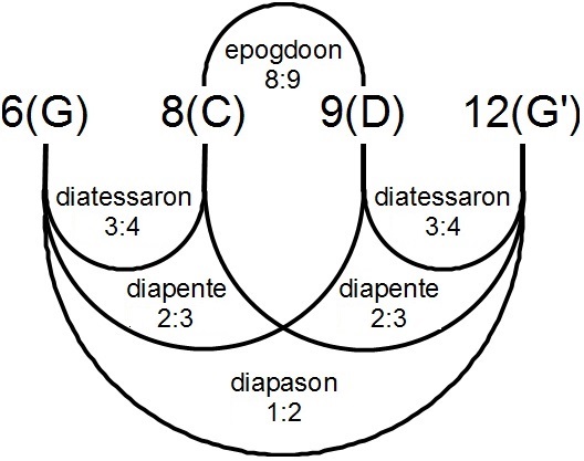
Figure 2: Pythagorean music theory: diagram showing relations between epogdoon, diatessaron, diapente, and diapason, which correspond to the Major Second (9/8), Perfect Fourth (4/3), Perfect Fifth (3/2) and Octave (2/1), respectively. Pythagorean length ratios in this figure are the multiplicative inverse of frequency relations as used in this article.

The four notes are also labeled harmonic consonances since they sound “pleasant” when played together. However, this property should not be understood just as a human perception, but as a consequence of the mathematical simple ratios that characterize these notes so that the subjective gradation from consonance to dissonance should correspond to a gradation of sound-frequency ratios from simple ratios to more complex ones. The International Cyclopedia of Music and Musicians (Thompson, 1946) explains: “Acoustically, consonance is the degrees of blending and fusion between two or more tones. The lower the ratio, such as 2:1, 3:2, 4:3, the greater the degree of fusion, hence consonance. Consonance may also be distinguished by the degree of freedom from beats. The octave (2:1) is the most perfect acoustic consonance and is free of beats; then follows, in order of degree, the fifth (3:2), the fourth (4:3), etc.; the series becoming more and more dissonant as the ratios depart from the simplest, i.e. 2:1.”

Several scientific works have linked the acoustics of consonances to their aesthetic qualities (Bones et al., 2014; McDermott et al., 2010; Plack, 2010). However, these ratios appear to have also a deep geometrical and physical meaning, which may explain why they may be relevant to reveal some hidden organization of the solar system and of other physical systems. For example, the four main tones of the Pythagorean musical set describe a Keplerian orbit. In fact, if $a$ is the semi-major axis, $b$ the semi-minor axis and $l=a(1-e^{2})$, it is found that $a$ is the arithmetic mean, $b$ the geometric mean and $l$ the harmonic mean of $r_{min}$ and $r_{max}$ (Cartwright et al., 2021).

In the 16th century, musical theorists such as Gioseffo Zarlino (1517–1590) completed the traditional set of harmonic consonances by adding four more intervals: the “Minor Third” (6/5); the “Major Third” (5/4); the “Minor Sixth” (8/5); and the “Major Sixth” (5/3) (Zarlino, 1558). These ratios can also be derived as harmonic and arithmetic means of 1/1 and 3/2 in the case of thirds and means between 4/3 and 2/1 in the case of sixths (Forster, 2010). The proposed system was defined as just because all notes are related by intervals that are defined by rational numbers (Cartwright et al., 2021). In the tuning systems employing just-intonation, exact harmonic consonance ratios are maximized.

In our analysis, we employ the five-limit twelve-tone scale which maximizes just intonation between tone pairs of the octave; we will refer to this as the twelve-tone just-intonation system (12-TJI). In this system, more complex ratios are assigned to the five remaining non-consonant (or dissonant) tones of the octave: (in the key of C) the “Minor Second” ($Db$, 16/15); the “Major Second” ($D$, 9/8); the “Tritone” ($Gb$, 45/32); the “Minor Seventh” ($Bd$, 9/5); and the “Major Seventh” ($B$, 15/8).

The utilization of perfect ratios of harmonic consonances within just-intonation tuning causes the size of half-steps to vary between different pairs of adjacent notes within the octave, as shown below. As a consequence, a keyboard instrument tuned to play in one key (e.g. $C$ major) can be wildly out of tune in another (e.g. $Gb$ major).

In order to minimize this limitation, different tuning systems evolved through the centuries, eventually yielding the twelve-tone equal-temperament (12-TET) system which, today, has been widely adopted. In general, an equal-tempered system is a musical tuning system that approximates just intervals by dividing an octave into equal steps. Therefore, the ratio of the frequencies of any adjacent pair of notes is the same. In the 12-TET, the smallest interval is a 1/12th of the width of an octave, and it is called a semitone or half-step. By normalizing the ratio of all half-steps in the octave to a value of

$$\gamma=2^{1/12}\approx 1.05946,$$ (4)

one can play equally in tune in any key (e.g. $C$ major, $Gb$ major, etc.), but this is achieved at the expense of introducing slight errors into all the perfect simple ratios of harmonic consonances, except the Unison and the Octave. A 12-TET system would have been unimaginable to ancient Greek philosophers because it involved roots of 2 which are irrational numbers.

To evaluate quantitatively how well specific tone pairs are tuned in the standard 12-TET system versus those in the 12-TJI system, the octave (that is the 2/1 ratio) is assumed to be made of 1200 cents. Given a real number $x$ between 1 and 2, its musical cent (MC) value is defined by the equation:

$$MC(x)=1200\log_{2}(x).$$ (5)

Thus, for $r=1$ (Unison) its MC value is 0 cents, while for $r=2$ (Octave) its MC value is 1200 cents. Moving sequentially by $n$ equal-tempered half-steps from a reference tone to a new tone, the frequency ratio between the two tones is exactly $\gamma^{n}=2^{n/12}$ so that its MC value is $100\times n$. If $r$ is larger than 2, Eq. 5 can still be used, and the correct tone relation can be estimated by subtracting an integer number of 1200 cents for each octave. For example, $MC=1200+100\times n$ cents ($x=2^{1+n/12}$) corresponds to the $n^{th}$ equal-tempered tone in the second octave; $MC=2400+100\times n$ cents ($x=2^{2+n/12}$) corresponds to the $n^{th}$ equal-tempered tone in the third octave; and so on.

In the idealized 12-TJI system, which uses the whole number ratios of harmonic consonances, the tones slightly diverge from the 12-TET ones: for example, a Perfect Fifth, a 3/2 ratio, has 702 cents while the 7 (equal-tempered) half-steps approximates a Perfect Fifth with $2^{7/12}$, which corresponds to 700 cents; similarly, a Major Third is 5/4 and corresponds to 386 cents, whereas 4 equal-tempered half-steps correspond to 400 cents; and so on. The differences between the 12-TJI and the 12-TET vary from 0 to 18 cents, with an average of 9 cents. Table 1 summarizes and compares the 12 tones in the 12-TET and 12-TJI systems.

The same MC notation can also be used to evaluate how close the ratios of orbital parameters between adjacent planets are to those of musical tones pairs in the 12-TJI and 12-TET systems.

In the following we will use both tuning systems: the 12-TJI allows a direct interpretation based on harmonic whole number ratios that recalls the resonance formalism of the orbital commensurabilities; the 12-TET system allows us to write the equations in a more compact mathematical formalism.

3 Basic attempts to find musical tones and consonances in the orbital parameter ratios of adjacent planets

In Harmonices Mundi Kepler (1619) attempted to find correspondences between ratios of planetary orbital parameters, musical harmony, and Platonic solids. Herein, we evaluate and study the ratios of the semi-major axis, sidereal periods, and mean orbital velocities of neighboring planets, including the asteroid belt.

The analysis aims to determine whether musical tones and, more specifically, consonances exist in such a series of orbital variables as found, for example, in the Trappist-1 solar system or among the moons of Jupiter. Table 2 reports the astronomical data herein used. The planets are listed from the closest to the farther from the Sun as: Mercury (Me); Venus (Ve); Earth (Ea); Mars (Ma); Asteroid (As); Jupiter (Ju); Saturn (Sa); Uranus (Ur); and Neptune (Ne).

Planet	S-M Axis	Period	Speed	$a^{2/3}$
	AU	year	km/s
Mercury	0.387	0.241	47.36	0.531
Venus	0.723	0.615	35.02	0.806
Earth	1.000	1.000	29.78	1.000
Mars	1.524	1.881	24.07	1.324
Asteroid	2.825	* 4.748	* 17.72	1.998
Jupiter	5.204	11.862	13.06	3.003
Saturn	9.583	29.457	9.68	4.512
Uranus	19.201	84.011	6.80	7.170
Neptune	30.048	164.79	5.43	9.665

Table 2: The semi-major axes $a$, sidereal period $T$ and mean orbital velocities $v$ of the planets of the solar system, including the belt of the asteroids located between Mars and Jupiter. Asteroid refers to the 5:2 Kirkwood asteroid-belt gap; (*) indicates theoretical values calculated using Eq. 1. The last column reports the values of $a^{2/3}$ discussed in the main text. (Data from: https://nssdc.gsfc.nasa.gov/planetary/factsheet/).

The asteroid belt distance from the Sun (As) was set at the 5:2 Kirkwood-gap ($2.825$ AU) as a surrogate (although negative or missing) planet because, in the following discussion, such a region is supposed to be a kind of “divergence” or “reflection” point separating the inner (or terrestrial) from the outer (or gas-giant) planets (cf.: Geddes and King-Hele, 1983; Moons and Morbidelli, 1995). This is the central gap of the asteroid belt and it is linked to the 5:2 resonance between Jupiter and Saturn. Such a distance is very close to the geometrical mean between Mars and Jupiter, $\sqrt{Ma\times Ju}\approx 2.816$ AU, and to the mean orbital radius of the dwarf planet Ceres (about $2.769$ AU).

Planets	Ratio	MC	12-TET	(Con)	ET-MCerr	12-TJI	(Con)	JI-MCerr
Semi-Major Axis Length
Ve/Me	1.868	1082	$B$	(N)	-18	$B$	(N)	-6
Ea/Ve	1.383	562	$Gb$	(N)	-38	$Gb$	(N)	-28
Ma/Ea	1.524	729	$G$	(Y)	29	$G$	(Y)	27
As/Ma	1.854	1068	$B$	(N)	-32	$B$	(N)	-20
Ju/As	1.842	1058	$B$	(N)	-42	$B$	(N)	-30
Sa/Ju	1.841	1057	$B$	(N)	-43	$Bb$/$B$	(N)	31/-31
Ur/Sa	2.004	1203	$C$	(Y)	3	$C$	(Y)	3
Ne/Ur	1.565	775	$Ab$	(Y)	-25	$Ab$	(Y)	-39
Orbital Period
Ve/Me	2.552	* 422	$E$	(Y)	22	$E$	(Y)	36
Ea/Ve	1.626	842	$Ab$	(Y)	42	$Ab$	(Y)	28
Ma/Ea	1.881	1094	$B$	(N)	-6	$B$	(N)	6
As/Ma	2.524	* 403	$E$	(Y)	3	$E$	(Y)	17
Ju/As	2.498	* 385	$E$	(Y)	-15	$E$	(Y)	-1
Sa/Ju	2.484	* 375	$E$	(Y)	-25	$E$	(Y)	-11
Ur/Sa	2.852	* 614	$Gb$	(N)	14	$Gb$	(N)	24
Ne/Ur	1.962	1166	$C$	(Y)	-34	$C$	(Y)	-34
Average Orbital Speed
Me/Ve	1.352	523	$F$	(Y)	23	$F$	(Y)	25
Ve/Ea	1.176	281	$Eb$	(Y)	-19	$Eb$	(Y)	-35
Ea/Ma	1.237	369	$E$	(Y)	-31	$E$	(Y)	-17
Ma/As	1.358	530	$F$	(Y)	30	$F$	(Y)	32
As/Ju	1.357	529	$F$	(Y)	29	$F$	(Y)	31
Ju/Sa	1.349	518	$F$	(Y)	18	$F$	(Y)	20
Sa/Ur	1.424	611	$Gb$	(N)	11	$Gb$	(N)	21
Ur/Ne	1.252	389	$E$	(Y)	-11	$E$	(Y)	3

Table 3: Musical tones in the semi-major axis, orbital period, average speed ratios of adjacent planets. The columns indicate: the adjacent planet couples; the orbital parameter ratio; its value in musical cents (MC), the symbol (*) indicates that the MC value is reduced by 1200 cents; 12-TET is the closest tone (for the inner planet of the pair when the outer planet is tuned to $C$) according to the exact 12-TET system with the Yes/No consonance property (Con); ET-MC_err is the relative error; 12-TJI and JI-MC_err are equivalent but relative to the 12 tones of the just-intonation 12-TJI system. (Refer to Table 1 for the numerical values of the tones).

Table 3 shows the chosen orbital ratios, their values in MC (using Eq. 5), and their closest tone (using Table 1) relative to both the 12-TET and the 12-TJI systems. In addition, we report in parenthesis whether or not the closest tone is a consonance and the error-distance in MC of the planetary ratio from the closest tone for both musical systems. Here we maintain Kepler’s practice of assigning the higher frequency tone to the faster moving, inner planet. We also assume that when the discrepancy between the orbital ratio and the music tone is equal or larger than 25 cents, the two values are not compatible (let us say “untuned”) and, therefore, such an orbital ratio cannot be interpreted as a musical tone in these tuning systems.

Table 3 shows that out of 8 planetary adjacent couples:

• using the semi-major axis – 6 or 5 ratios, in 12-TET and 12-TJI respectively, are untuned, and only 3 are close to consonances, of which 2 are untuned.

• using the orbital period – 3 ratios are untuned, and only 6 are close to consonances, of which 3 are untuned.

• using the average speed – 3 or 4 ratios are untuned, and only 7 are close to consonances, of which 3 or 4 are untuned, respectively.

Thus, the results are not satisfactory as each of these three metrics fails to find tuned musical correlates for several planetary pair ratios. However, one could wonder whether a different set of orbital measures could provide a better musical interpretation of the movements of the bodies of the solar system.

In this regard, we notice that Kepler’s third law of planetary motions (Eq. 1) indicates the existence of simple relations between the ratios of planetary measurements, which are characterized by specific exponents such as

$$\left\{\begin{array}[]{lll}(a_{1}/a_{2})^{3/2}&=&T_{1}/T_{2}\\ (a_{1}/a_{2})^{-1/2}&=&v_{1}/v_{2},\end{array}\right.$$ (6)

where the first equation derives directly from Kepler’s third law and the second by approximating the orbital perimeter as $2\pi a$, where $a$ is the semi-major axis, and using the definition of mean orbital speed as $v=2\pi a/T$. Thus, the ratios of average distances, orbital periods, and average velocities are mutually related by varying the exponents from $1$, to $3/2$, to $-1/2$ respectively.

Thus, in the following sections, we look for exponents $k$ such that the values

$$(a_{1}/a_{2})^{k}$$ (7)

for adjacent planets could be best expressed in musical tones and, more specifically, in harmonic consonances. To do this, we take advantage of the equations proposed by Geddes and King-Hele (1983).

4 The Geddes – King-Hele equations

Geddes and King-Hele (1983) noted that the orbits of the eight planets of the solar system appear as if they were “reflected” about the asteroid belt so that the following symmetries are found: Mercury$\leftrightarrow$Neptune, Venus$\leftrightarrow$Uranus, Earth$\leftrightarrow$Saturn, and Mars$\leftrightarrow$Jupiter.

More specifically, these authors found that the ratios among the mean distances from the Sun of the planets (in the following denoted by the planet’s name initials) could be approximated as powers of a single constant which these authors denoted by

$$r=2^{1/8}\approx 1.09051.$$ (8)

Then, the following nearly exact equations relating contiguous planets were found:

$$\left\{\begin{array}[]{lll}Ve\approx r^{7}Me;&Ea\approx r^{4}Ve;&Ma\approx r^{5}Ea;\\ As\approx r^{7}Ma;&Ju\approx r^{7}As;\\ Sa\approx r^{7}Ju;&Ur\approx r^{8}Sa;&Ne\approx r^{5}Ur.\end{array}\right.$$ (9)

The middle equations relate Mars, an estimate of the asteroid belt distance from the Sun and Jupiter, where the distance of the asteroid belt ($As$) was originally arbitrarily set at $\sqrt{Ma\times Ju}\approx 2.816$ AU, which is, nevertheless, very close to the 5:2 Kirkwood-gap at $2.825$ AU that we prefer to use in the following as the mirror point.

Geddes and King-Hele (1983) noted that the percent errors in the eight equations listed in the system 9 are very small. We get: 1.9%, -2.2%, -1.2%, 0.8%, 0.8%, 0.4%, 0.2%, 1.5% respectively.

The above equations can also be combined in several ways. For example, it is possible to obtain the mean distance from the Sun of all planets as a function of only that of Mercury and specific powers of $r$. It is also easy to obtain the following identity:

$$\frac{Ve\times Ju}{Me\times Sa}\approx\frac{Ea\times Ne}{Ma\times Ur}\approx 1,$$ (10)

which have an accuracy of 1.5% and 2.7%, respectively. Finally, it is possible to obtain the following Geddes – King-Hele equations that “mirror” the planets relative to the asteroid belt:

$$\frac{Me}{Ea}\times\frac{Ne}{Sa}\approx\frac{Ve}{Me}\times\frac{Ur}{Ne}\approx\frac{Ea}{Ma}\times\frac{Sa}{Ju}\approx r^{2}=2^{1/4}$$ (11)

$$\frac{Sa}{Ea}\times\frac{Ma}{Ju}\approx\frac{Ur}{Ve}\times\frac{Ea}{Sa}\approx\frac{Ne}{Me}\times\frac{Ve}{Ur}\approx r^{12}=2^{3/2}$$ (12)

It is to be noted that the chosen constant $r$ was interpreted by the authors as the mean frequency ratio between notes in a musical octave, although Abhyankar (1983) critiqued such an interpretation. However, as explained above, in Western musical practice, the octave is divided into 12 parts, not 8.

5 A non-linear transformation of the Geddes – King-Hele equations

Herein we convert the Geddes – King-Hele equations to a form that is compatible with the chromatic musical scale. This is done by raising each side of Eqs. 9 to the $k=2/3$ power. In fact, as previously stated, the frequency ratio between any adjacent half-steps in the 12-TET system is $\gamma=2^{1/12}\approx 1.05946$ (Eq. 4), which is equal to $r^{2/3}$.

Abhyankar (1983) also noted that such a change of metric would make the Geddes – King-Hele equations more compatible with the frequency ratios between the notes of the tuning systems proposed above. However, he summarily and erroneously concluded that there was “nothing particularly musical” about the mirror-symmetries between the distances of the planets nor that those symmetries were “telling us something about the origin of the Solar System or its stability”. Indeed, he did not realize the mathematical and physical properties of the new equations that the new metric implies. Let us disclose it.

The new planetary terms can now be related mathematically by powers of $\gamma$, which is equivalent to movements in half-steps in the 12-TET musical system because $\gamma=r^{2/3}$. Therefore, it follows that:

$$\left\{\begin{array}[]{lll}Ve^{\prime}\approx\gamma^{7}Me^{\prime};&Ea^{\prime}\approx\gamma{}^{4}Ve^{\prime};&Ma^{\prime}\approx\gamma{}^{5}Ea^{\prime};\\ As^{\prime}\approx\gamma{}^{7}Ma^{\prime};&Ju^{\prime}\approx\gamma{}^{7}As^{\prime};\\ Sa^{\prime}\approx\gamma{}^{7}Ju^{\prime};&Ur^{\prime}\approx\gamma{}^{8}Sa^{\prime};&Ne^{\prime}\approx\gamma{}^{5}Ur^{\prime}.\end{array}\right.$$ (13)

where $Me^{\prime}=Me^{2/3}$, $Ve^{\prime}=Ve^{2/3}$, $Ea^{\prime}=Ea^{2/3}$, $Ma^{\prime}=Ma^{2/3}$, $As^{\prime}=As^{2/3}$, $Ju^{\prime}=Ju^{2/3}$, $Sa^{\prime}=Sa^{2/3}$, $Ur^{\prime}=Ur^{2/3}$and $Ne^{\prime}=Ne^{2/3}$.

We can now employ the 12-TET system to express the ratios between adjacent planets in terms of musical half-steps. For example, $Ve^{\prime}=\gamma^{7}Me^{\prime}$ can be rewritten as:

$$\left(\frac{Ve}{Me}\right)^{\frac{2}{3}}=\frac{Ve^{\prime}}{Me^{\prime}}\approx\gamma^{7}=2^{7/12}.$$ (14)

This is equivalent to saying that the ratio of semi-major axis lengths of the orbits of Venus and Mars elevated to the 2/3rd power, that is $Ve^{\prime}/Me^{\prime}$, is equal to the ratio of frequencies of two pitches that are 7 half-steps apart, which corresponds to a Perfect Fifth (a ratio of 3/2).

Eq. 12 can be rewritten as:

$$\frac{Sa^{\prime}}{Ea^{\prime}}\times\frac{Ma^{\prime}}{Ju^{\prime}}\approx\frac{Ur^{\prime}}{Ve^{\prime}}\times\frac{Ea^{\prime}}{Sa^{\prime}}\approx\frac{Ne^{\prime}}{Me^{\prime}}\times\frac{Ve^{\prime}}{Ur^{\prime}}\approx\gamma^{12}=2,$$ (15)

which expresses octave ratios.

Abhyankar (1983) was able to derive Eq. 15, but he did not realize that it implies a series of scaling musical relations. In fact: $Ju^{\prime}/Ma^{\prime}\approx\gamma^{14}$ = 14 half-steps $\approx$ 2 Perfect Fifths = $\left(3/2\right)\times\left(3/2\right)=2.25$; $Sa^{\prime}/Ea^{\prime}$ adds an octave to that, doubling the ratio to 4.5; similarly, $Ur^{\prime}/Ve^{\prime}$ doubles this to 9; and $Ne^{\prime}/Me^{\prime}$ doubles that to 18. Consequently, Eq. 15 can be rewritten also in the following compact form:

$$1\frac{Ne^{\prime}}{Me^{\prime}}\approx 2\frac{Ur^{\prime}}{Ve^{\prime}}\approx 4\frac{Sa^{\prime}}{Ea^{\prime}}\approx 8\frac{Ju^{\prime}}{Ma^{\prime}}\approx 18,$$ (16)

which reveals, both a mirror-like and scaling structure relative to the asteroid belt. Note the sequence of the powers of 2 ($1=2^{0}$, $2=2^{1}$, $4=2^{2}$ and $8=2^{3}$) relative to planetary pairs approaching the asteroid belt.

As a function of the semi-major axis $a$, of the period $T$ and of the mean orbital speed $v$, Eq. 16 corresponds to

$$1\left(\frac{a_{Ne}}{a_{Me}}\right)^{\frac{2}{3}}\approx 2\left(\frac{a_{Ur}}{a_{Ve}}\right)^{\frac{2}{3}}\approx 4\left(\frac{a_{Sa}}{a_{Ea}}\right)^{\frac{2}{3}}\approx 8\left(\frac{a_{Ju}}{a_{Ma}}\right)^{\frac{2}{3}} \approx 18$$ (17)

$$1\left(\frac{T_{Ne}}{T_{Me}}\right)^{\frac{4}{9}}\approx 2\left(\frac{T_{Ur}}{T_{Ve}}\right)^{\frac{4}{9}}\approx 4\left(\frac{T_{Sa}}{T_{Ea}}\right)^{\frac{4}{9}}\approx 8\left(\frac{T_{Ju}}{T_{Ma}}\right)^{\frac{4}{9}} \approx 18$$ (18)

$$1\left(\frac{v_{Me}}{v_{Ne}}\right)^{\frac{4}{3}}\approx 2\left(\frac{v_{Ve}}{v_{Ur}}\right)^{\frac{4}{3}}\approx 4\left(\frac{v_{Ea}}{v_{Sa}}\right)^{\frac{4}{3}}\approx 8\left(\frac{v_{Ma}}{v_{Ju}}\right)^{\frac{4}{3}} \approx 18$$ (19)

where the Eqs. 6 were used. Using Table 2, the exact values of the four ratios multiplied by increasing powers of 2 are: 18.20, 17.80, 18.05 and 18.14, respectively, using the semi-major orbital axes; 18.20, 17.79, 17.99 and 18.14, respectively, using the periods; and 17.95, 17.79, 17.90 and 18.08, respectively, using the mean orbital velocities. Thus, Eq. 16 [or Eqs. 17, 18 and 19] describes the orbits of the planets of the solar system within about $1\%$ error (or with a 99% accuracy), and elegantly expresses its scaling and mirror-like symmetry structure with respect to the asteroid belt. More sprecifically, it suggests that the inner and outer orbits of the solar system are organized in a simple scaling structure.

Using the equations for planetary distances raised to the 2/3rd power and expressing the results in terms of half-steps, we now evaluate how well the planetary ratios can be assigned to musical tones.

Planets	Ratio	Ratio2/3	MC	NHS	Tone and Consonance			ET-MC	ET-MCerr	JI-MC	JI-MCerr
Ve/Me	1.868	1.517	721	7	$G$	Perfect Fifth	(Y)	700	21	702 ($3/2$)	19
Ea/Ve	1.383	1.241	374	4	$E$	Major Third	(Y)	400	-26	386 ($5/4$)	-12
Ma/Ea	1.524	1.324	486	5	$F$	Perfect Fourth	(Y)	500	-14	498 ($4/3$)	-12
As/Ma	1.854	1.509	712	7	$G$	Perfect Fifth	(Y)	700	12	702 ($3/2$)	10
Ju/As	1.842	1.503	705	7	$G$	Perfect Fifth	(Y)	700	5	702 ($3/2$)	3
Sa/Ju	1.841	1.502	705	7	$G$	Perfect Fifth	(Y)	700	5	702 ($3/2$)	3
Ur/Sa	2.004	1.589	802	8	$Ab$	Minor sixth	(Y)	800	2	814 ($8/5$)	-12
Ne/Ur	1.565	1.348	517	5	$F$	Perfect Fourth	(Y)	500	17	498 ($4/3$)	19

Table 4: Number of half-steps (NHS), musical tones and consonances in both the exact 12-TET (ET) and 12-TJI (JI) values, and in musical cents (MC), versus the semi-major axis ratios of adjacent planets elevated to the 2/3rd power, with the relative musical cent errors (MC_err). (Refer to Table 1 for the numerical values of the tones).

Table 4 reports the semi-major axis ratios of adjacent planets elevated to the 2/3rd power using the orbital data listed in Table 2, and compares them with their closest musical tones using both the 12-TET and 12-TJI values (expressed in musical cents, using Eq. 5). We also tabulated the relative musical cent errors from the closest tone. Figure 3 shows the results using both tone systems.

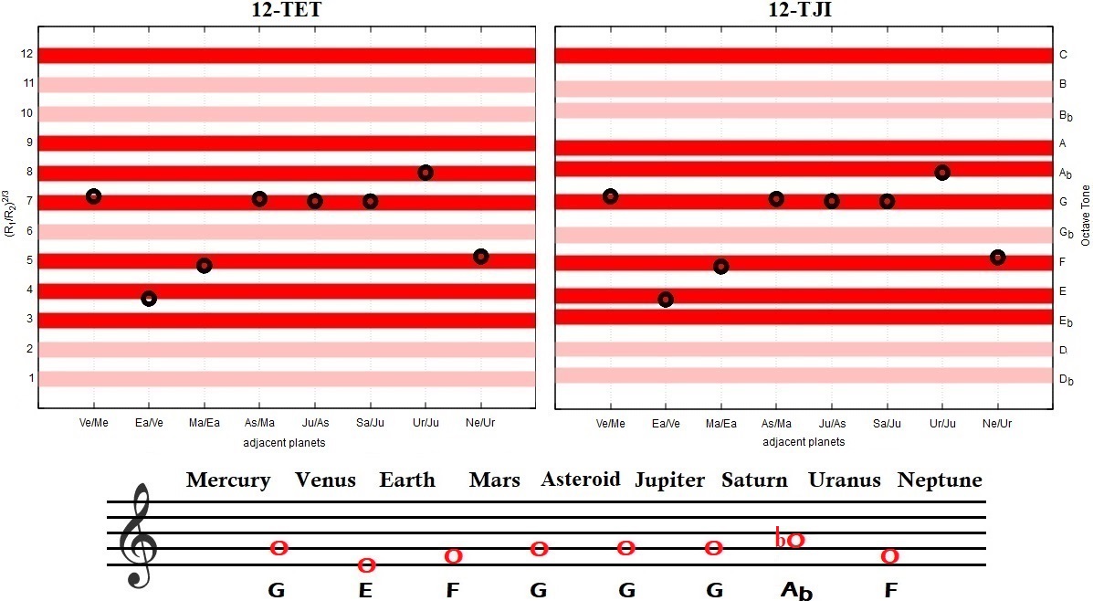
Figure 3: Top: The black circles indicate the distance ratios raised to the 2/3rds power of adjacent planets in both the equal tempered 12-TET and justly tuned 12-TJI (in the key of $C$ expressed as half-steps or MC/100): see Table 4. The red bars indicate the consonances, while the pink ones the dissonances. The width of each bar is 50 cents. Bottom: the musical notation gives the note for the inner planet of the pair when the outer planet is tuned to middle $C$. (Refer to Table 1 for the numerical values of the tones).

Using the 12-TET system, an absolute divergence between 2 and 26 cents, with an average of 13 cents is observed; whereas in the 12-TJI tuning, the absolute divergence is between 3 and 19 cents, with an average of 11 cents. These results suggest that the chosen planetary measure among couples of adjacent planets of the solar system can be well approximated by the tones of the Western musical tradition.

As previously stated, of the 12 possible tones within the octave, 7 are considered consonances (Stephenson, 1974). This happens when the exact value of the note can be well approximated by a ratio $n/m$ where the whole numbers $n$ and $m$ are small and members of the set: 3, 5, and powers of 2. The consonance ratios, in the key of $C$, are: Unison or Octave ($C$), 1/1 or 2/1; Minor Third ($Eb$), 6/5; Major Third ($E$), 5/4; Perfect Fourth ($F$), 4/3; Perfect Fifth ($G$), 3/2; Minor Sixth ($Ab$), 8/5; Major Sixth ($A$), 5/3. As summarized in Table 5, $Ve^{\prime}/Me^{\prime}$, $As^{\prime}/Ma^{\prime}$, $Ju^{\prime}/As^{\prime}$, and $Sa^{\prime}/Ju^{\prime}$ are tuned to a Perfect Fifth, $Ma^{\prime}/Ea^{\prime}$ and $Ne^{\prime}/Ur^{\prime}$ are tuned to a Perfect Fourth, $Ea^{\prime}/Ve^{\prime}$ is tuned to a Major Third, and $Ur^{\prime}/Sa^{\prime}$ to a Minor Sixth.

#	Name	Tone	Consonance	Planet ratio
1	Minor second	$Db$	No
2	Major second	$D$	No
3	Minor third	$Eb$	Yes
4	Major Third	$E$	Yes	$Ea^{\prime}/Ve^{\prime}$
5	Perfect Fourth	$F$	Yes	$Ma^{\prime}/Ea^{\prime}$; $Ne^{\prime}/Ur^{\prime}$
6	Tritone	$Gb$	No
7	Perfect Fifth	$G$	Yes	$Ve^{\prime}/Me^{\prime}$; $As^{\prime}/Ma^{\prime}$;
				$Ju^{\prime}/As^{\prime}$; $Sa^{\prime}/Ju^{\prime}$
8	Minor sixth	$Ab$	Yes	$Ur^{\prime}/Sa^{\prime}$
9	Major Sixth	$A$	Yes
10	Minor seventh	$Bb$	No
11	Major Seventh	$B$	No
12	Octave	$C$	Yes

Table 5: Comparison between the 12 tones and the semimajor axis ratios among the adjacent planets raised to the $k=2/3$ power deduced from the corrected Geddes–King-Hele planetary distance equations (Eq. 13). The tone is that of the inner planet of the pair when the outer planet is tuned to C. (Refer to Table 1 for the numerical values of the tones).

Thus, not only do all these planetary ratios appear sufficiently well-tuned to be members of the traditional music octave, but all of them also correspond to the musical consonance ratios according to both the 12-TET and 12-TJI systems. This result suggests that, taken as a set, the orbits of the planets present a specific well tuned and harmonized structure.

6 Statistical significance and robustness of the exponent k = 2/3

We now check whether the close fit between idealized musical ratios and planetary data using the exponent $k=2/3$ is coincidental. Thus, we repeated the above calculations by varying the value of $k$ between 0.3 to 1 in steps of 0.001.

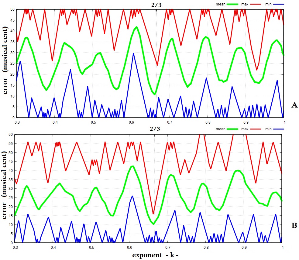
Figure 4: Exponent $k$ versus average, maximum and minimum error measured in musical cents from adjacent planet distance ratios raised to the exponent $k$ to the closest musical tone for: A) the equal tempered 12-TET system; B) the justly tuned 12-TJI. The value for $k=2/3\approx 0.667$ is highlighted.

Figure 4 plots the average, maximum and minimum error (measured in MC) between the eight adjacent planet semi-major axis ratios raised to the power of $k$ and the closest of the twelve musical tones listed in Table 1 as a function of the exponent $k$. Figure 4A uses the tones of the 12-TET system while Figure 4B uses those of the 12-TJI system. The analysis depicted in Figure 5 uses only the 7 consonances and ignores the other 5 tones. The position of the value for $k=2/3$ is highlighted in both figures.

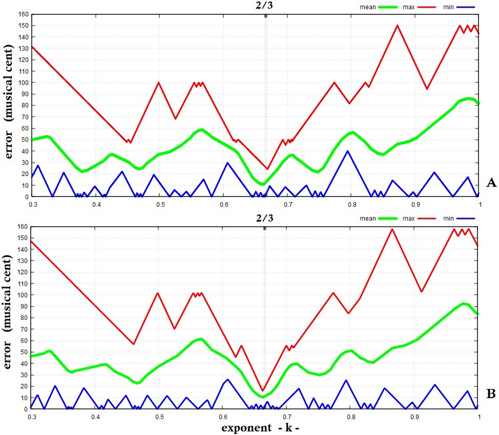
Figure 5: Exponent $k$ versus average, maximum and minimum error measured in musical cents from adjacent planet distance ratios raised to the exponent $k$ to the closest musical consonance for: A) 12-TET system; B) the 12-TJI system. The value for $k=2/3\approx 0.667$ is highlighted.

Figures 4 and 5 show that $k\approx 2/3$ corresponds to the absolute minimum in the average error (green curve) between our proposed model and both musical tuning systems, which suggests that the chosen measure could be physically meaningful. Regarding the maximal error (red curve), $k\approx 2/3$ corresponds in Figure 4A to the second-lowest minimum, and to the absolute minimum in Figure 4B and in both Figures 5A and 5B, which refer to the consonances alone. The result suggests that the exponent $k=2/3$ optimizes the metrics expressed by Eq. 7 to reproduce the simple ratios found in musical consonances.

To further test the statistical relevance of our result, we now evaluate the probability of obtaining the 8 planetary ratios close to musical consonances against the null hypothesis that they are randomly distributed. Above we found that the planetary data yield the simple ratios of harmonic consonances within a mean accuracy of about 11-13 cents up to a maximum of 26 cents in just a single case relative to the 12-TET system. The range in MC of planetary distance ratios elevated to the 2/3rd power is 428 cents: from 374 cents (close to a Major Third for Ea’/Ve’) to 802 cents (close to a Minor Sixth for Ur’/Sa’). To each end of this range, we add the associated error-value, to obtain a total band range of 475 cents from 350 to 825 cents. Within this range, four idealized consonance ratios lie: the Major Third, the Perfect Fourth, the Perfect Fifth, and the Minor Sixth. Each of these four tones can be assumed to have a maximum error range of $\pm$25 cents. Therefore, their total error range accommodates at most 200 cents of the total available 475 cent range, that is 50 cents for each of the four consonances. Thus, the statistical chance that the eight planetary ratios occur randomly with this proximity to the four selected consonances is $p=(200/475)^{8}<0.001=0.1\%$. Thus, it is very unlikely that our result occurs by chance.

7 Comparison versus the harmonic orbit resonance model

Aschwanden (2018) studied the regularity of the spaced patterns of the distances of the planets of the solar system and showed that logarithmic spacing models, such as both the Titus-Bode law and its generalized form, perform poorly versus a harmonic resonance model based on quantized scaling factors. More specifically, the author showed that the planet distances $R_{i}$ from the Sun and their orbital periods $T_{i}$ (where $i=1$ for Mercury, $i=2$ for Venus, etc.) are related to scaling laws of the type:

$$\frac{R_{i+1}}{R_{i}}=\left(\frac{T_{i+1}}{T_{i}}\right)^{\frac{2}{3}}=\left(\frac{H_{i+1}}{H_{i}}\right)^{\frac{2}{3}}$$ (20)

where the $2/3$ exponent derives from Eq. 1, and the whole number ratios $H_{i+1}/H_{i}$ yield to the following planetary equations linking the semi-major axes of neighboring planet pairs:

$$\left\{\begin{array}[]{ll}Ve\approx(5/2)^{2/3}Me;&Ea\approx(5/3)^{2/3}Ve;\\ Ma\approx(2/1)^{2/3}Ea;&As\approx(5/2)^{2/3}Ma;\\ Ju\approx(5/2)^{2/3}As;&Sa\approx(5/2)^{2/3}Ju;\\ Ur^{\prime}\approx(3/1)^{2/3}Sa;&Ne\approx(2/1)^{2/3}Ur.\end{array}\right.$$ (21)

The Eqs. 21 express a planetary model of the solar system alternative to that of Eqs. 13. The scaling factors are different. Thus, it is important to determine which one of the two planetary models performs better in predicting the size of the orbits of the solar system.

To do this, we observe that given a semi-major axis $a$ for a planet (see Table 2), the equation sets 13 and 21 can be used to predict the position of the other eight planets relative to the chosen one. Thus, for each of the two models, we can obtain nine different sets of predictions starting from each planet. Finally, the two prediction groups are statistically compared.

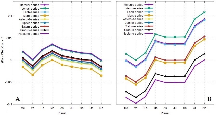
Figure 6: Relative errors regarding the predictions of the semi-major axis lengths of the planets of the solar system according to: [A] the Geddes – King-Hele 12-TET based model (Eqs. 13) herein proposed; [B] the harmonic orbit resonance model by Aschwanden (2018) (Eqs. 21).

This is done in Figure 6 that shows the relative error for each planet given by the expression:

$$relative\;error=\frac{prediction-observation}{observation}-1.$$ (22)

The figure shows that the Geddes – King-Hele 12-TET based model (Eqs. 13) performs significantly better than the harmonic orbit resonance model by Aschwanden (2018) (Eqs. 21). This is demonstrated by the lower dispersion and trend bias in the relative error sets produced by the former model relative to the latter one. Table 6 reports the average predictions for each planet relative to the nine sets for each model with the relative errors relative to the observations. It is found that on average the Geddes – King-Hele 12-TET model predicts the correct semi-major axis lengths with a mean error of 0.8%, while the harmonic orbit resonance model has a mean error of 2.5%. The latter also presents a trend bias because the semi-major axis lengths of Mercury, Venus and Earth are underestimated by about 4% while those of Uranus and Neptune are overestimated by about 5%.

Planet	S-M Axis	GKH 12-TET		HOR
	Observations	Predictions	Error (%)	Predictions	Error (%)
Mercury	0.387	0.388	0.26	0.374	-3.26
Venus	0.723	0.712	-1.58	0.690	-4.62
Earth	1.000	1.006	0.63	0.969	-3.06
Mars	1.524	1.552	1.83	1.539	0.97
Asteroid	2.825	2.846	0.75	2.834	0.34
Jupiter	5.204	5.220	0.31	5.221	0.33
Saturn	9.583	9.574	-0.10	9.617	0.36
Uranus	19.201	19.147	-0.28	20.005	4.19
Neptune	30.048	29.529	-1.73	31.756	5.68

Table 6: Mean predictions and relative errors in the semi-major axes of the planets of the solar system relative to: [A] the Geddes – King-Hele 12-TET based model (Eqs. 13) herein proposed; [B] the harmonic orbit resonance (HOR) model by Aschwanden (2018) (Eqs. 21).

The poor performance of the harmonic orbit resonance model was somewhat expected from the results discussed in section 3 because it approximates the orbital period ratios listed in Table 3 with consonances (within two octaves), which, however, are not always the closest of the twelve tones to the period ratios. Even if the harmonic orbit resonance model would have adopted the more accurate ratios listed in Table 3, it would have nevertheless inadequately agreed with the data, as we discussed in Section 3.

8 Prediction of the Kirkwood gaps of the asteroid-belt

As a final test, we extend the Geddes – King-Hele 12-TET model to evaluate its prediction ability. For example, the increasing powers of 2 present in Eq. 17 as the planet pairs approach the mirror point given by the asteroid belt, suggest the existence of a final step characterized by the multiplicative factor $2^{4}=16$, which is the highest possible value compatible with the constant 18 that satisfies the condition $a_{i+1}/a_{i}>1$.

This extension suggests the existence of one last inner pair of close orbits (semi-major axis $a_{1}<a_{2}$) that are mirror-symmetric relative to the asteroid belt and that fulfill the following condition:

$$16\left(\frac{a_{2}}{a_{1}}\right)^{\frac{2}{3}}\approx 18.$$ (23)

Since the two orbits would be very close to each other, they should characterize the geometry of the asteroid belt itself. Note that the ratio $18/16=9/8$ corresponds to the Pythagorean epogdoon (Figure 2).

Indeed, the asteroid main-belt is characterized by five primary gaps at the 4:1, 3:1, 5:2, 7:3, 2:1 mean-motion resonances between the asteroids and Jupiter (Moons and Morbidelli, 1995; Moons et al., 1998). The central region is characterized by the three central gaps at $a_{3:1}=2.502$ AU, $a_{5:2}=2.825$ AU, and $a_{7:3}=2.958$ AU, respectively. Ceres is nearly in the middle at $a_{c}=2.769$ AU. By assuming the mirror point at Ceres or at $a_{5:2}$ (which is what we adopted above for the entire solar system), we have the possible mirroring pair given by $a_{3:1}\leftrightarrow a_{7:3}$. By applying Eq. 23, we get:

$$16\left(\frac{a_{7:3}}{a_{3:1}}\right)^{\frac{2}{3}}=16\left(\frac{3}{7}\times\frac{3}{1}\right)^{\frac{4}{9}}=16\left(\frac{9}{7}\right)^{\frac{4}{9}}=17.89,$$ (24)

where we used Eqs. 1 and 17, together with the period of Jupiter (11.86 years) to get $a_{3:1}$ and $a_{7:3}$. Thus, the prediction of Eq. 23 has an error of 0.6% and it is linked to Jupiter’s resonances.

It is interesting to notice that if the ratios $As/Ma$ and $Ju/As$ (where above we chose $As=a_{5:2}$ as the mirror point and the asteroid-belt position) are evaluated as $a_{3:1}/Ma$ and $Ju/a_{7:3}$, we would get 572 and 652 MC, respectively, which do not correspond to any tone and occur near 600 MC that corresponds to a Tritone (a dissonant tone relation). Perhaps, these relations explain why $a_{3:1}$ and $a_{7:3}$ are gaps despite their orbital resonance with Jupiter and, in general, why the asteroid belt occupies an unstable gravitational region.

In conclusion, Eq. 17 with its mathematical extension Eq. 23 appears to well characterize the regularity of the spaced patterns of the distances of the planets of the solar system including the inner main structure of the asteroid belt.

9 Vulcanoid asteroids versus transneptunian objects

Eq. 17 plus Eq. 23 should complete our model, which is, therefore, physically fully constrained. In fact, no other extension of the equation would be possible since it would require an additional, but unknown terrestrial planet between the Sun and Mercury — the mythical planet Vulcan that Urbain Le Verrier suggested in the 1850s to explain the anomalies of the orbit of Mercury (a problem that was later solved by Albert Einstein) or some vulcanoid asteroids which are still hypothesized (Evans et al., 1999) — and another planet between Neptune and the termination shock or the heliopause boundary (between 30 and 100 AU from the Sun) where only small transneptunian objects like Pluto, Eris, and other comets are found, which are not classified as regular planets of the solar system. Furthermore, it is not possible to extend our model beyond the gaps of the asteroid main-belt limit expressed by Eq. 23.

This property greatly differentiates our model from, for example, the Titius–Bode’s law whose upper limit (and also the lower limit in the case of Mercury) is unconstrained and, therefore, also yields questions of statistical robustness.

On the contrary, our equation is fully constrained. Thus, the statistical robustness of its predictions cannot be easily questioned, and it establishes that it is possible to evaluate the planetary orbits of the outer planets from those of the inner planets up to the gaps of the asteroid-belt with a single scaling and mirror-like equation (depicted graphically in Figure 7) within an average error of 1% or, alternatively, with a 99% accuracy.

In any case, let us try to extend the proposed model further; an operation that can be done by doubling and doubling again Eq. 17 for each pair of added symmetric bodies that, in the case of the solar system, can only generically represent astronomical bands, as actual real planets are missing.

By assuming Pluto ($a_{P}=39.237$ au), which could represent the Kuiper belt, and by doubling Eq. 17 to accommodate another planet pair, the semi-major axis of its specular body, the mythical planet Vulcan, would be expected at $a_{V}\approx 39.237/(18*2)^{3/2}=0.182$ au between the Sun and Mercury. Relative to their neighboring planets — Neptune and Mercury, respectively — we have $(a_{P}/Ne)^{2/3}=1.195\approx 6/5$ (Minor Third) and $(Me/a_{V})^{2/3}=1.65\approx 5/3$ (Major Sixth), which are both consonances.

By assuming Eris ($a_{E}=67.9$ au), which could represent the Scattered disk (a scarcely populated region at the boundary of the solar system), and by doubling again Eq. 17 to accommodate a second planet pair, its specular scattered disk would be expected at $a_{Sz}\approx 67.9/(18*4)^{3/2}=0.111$ au. Relative to their neighboring planets — Pluto and Vulcan, respectively — we have $(a_{E}/a_{P})^{2/3}=1.44\approx 45/32$ (Tritone) and $(a_{V}/a_{Sz})^{2/3}=1.39\approx 45/32$ (Tritone), which are both dissonant tones, as scattered regions would suggest.

Beyond the Scattered disk there is only the Oort cloud.

Thus, the Kuiper belt and the Scattered disk could be specular to the hypothesized vulcanoid asteroid belts and gaps, which could theoretically exist inside the orbit of Mercury at distances of 0.06-0.21 au from the Sun (Evans et al., 1999).

With the last considerations, we have completed the description of the solar system with a single scaling-mirror equation: Eq. 17 plus Eq. 23, plus its possible extensions obtained by doubling it for each pair of additional specular bodies or gravitational bands.

10 Discussion

The dynamics of celestial bodies follow the laws of gravitation complemented by some dissipative processes. The problem is that, even in the simplest case of three bodies interacting gravitationally, a closed-form solution for this case does not exist. However, empirical evidences suggest that orbital systems can self-organize in alternative synchronization structures which are not yet fully understood.

In the specific case of the solar system, we found that the rewriting of the Geddes – King-Hele equations in the proposed new form yields a very compact and elegant expression — Eq. 16 or, equivalently, Eqs. 17, 18, and 19 — which appears to disclose the hidden gravitational self-organization structure of our planetary system. When raised to the 2/3 power (a non-linear transformation), the orbits of the planets show a rational organization that is not apparent in the non-transformed orbital parameters. The fact that the 2/3 exponent minimizes the deviations and the planetary equations are more accurate than alternative harmonic resonance models, supports the robustness of our result.

Figure 7A graphically represents the orbital scaling and mirror-symmetries of the solar system in the following compact equation:

$$1\left(\frac{a_{Ne}}{a_{Me}}\right)^{\frac{2}{3}}\approx 2\left(\frac{a_{Ur}}{a_{Ve}}\right)^{\frac{2}{3}}\approx 4\left(\frac{a_{Sa}}{a_{Ea}}\right)^{\frac{2}{3}}\approx 8\left(\frac{a_{Ju}}{a_{Ma}}\right)^{\frac{2}{3}} \approx 16\left(\frac{a_{7:3}}{a_{3:1}}\right)^{\frac{2}{3}}\approx 18,$$ (25)

which links together the eight planets of the solar system plus the asteroid belt by highlighting the scaling and mirror symmetries among their semi-major axis lengths according to the 12-TET model of the Geddes – King-Hele equations. The above equation has a clear aesthetic appeal, and its five ratios have an accuracy of 99%.

Eq. 25 can also be further extended by doubling it for each pair of additional mirror-symmetric bodies. The first two possible extensions appear to have a physical meaning because they would correspond to the bands of the hypothesized vulcanoid asteroids versus the transneptunian objects and to the internal and external limits of the planetary disk of the solar system. According to this model, the planetary disk of the solar system would be constrained between two dissonant regions, that is a divergent or scattered zone very close to the sun (Sz) at about 0.1 au, and an equally divergent specular region corresponding to the Scattered disk (represented by Eris) and extending up to about 100 au from the sun. The asteroid belt, represented by Ceres, at about 2.0-3.5 au divides the planetary disk into an inner and outer region; this belt would also be a dissonant-divergent zone. Then, the inner region split into five rings would correspond to the orbits of Mars, Earth, Venus, Mercury, and, finally, the hypothesized Vulcanoid belt close to the sun. Similarly, the outer region split into five rings would correspond to the orbits of Jupiter, Saturn, Uranus, Neptune, and, finally, the Kuiper belt (represented by Pluto). In this way, the planetary disk of the Solar System would be fully described by the following extended mirror-scaling equation:

$$1\left(\frac{a_{Er}}{a_{Sz}}\right)^{\frac{2}{3}}\approx 2\left(\frac{a_{Pl}}{a_{Vu}}\right)^{\frac{2}{3}}\approx 4\left(\frac{a_{Ne}}{a_{Me}}\right)^{\frac{2}{3}}\approx 8\left(\frac{a_{Ur}}{a_{Ve}}\right)^{\frac{2}{3}}\approx$$

$$16\left(\frac{a_{Sa}}{a_{Ea}}\right)^{\frac{2}{3}}\approx 32\left(\frac{a_{Ju}}{a_{Ma}}\right)^{\frac{2}{3}} \approx 64\left(\frac{a_{7:3}}{a_{3:1}}\right)^{\frac{2}{3}}\approx 72,$$ (26)

which is shown in Figure 7B. The two sequences suggest that the orbital scaling-mirror symmetries of the solar system are expressed by the Pythagorean epogdoon (the tone ratio $9/8=18/16=72/64$) and its addition with one or more octaves.

Table 7 summaries the value and accuracy of each element of Eq. 26 obtained with the orbital data in Table 2. The equation was divided by 64 for normalization. We found that each planetary-pair ratio differs from the Pythagorean epogdoon (9/8) by at most 1%.

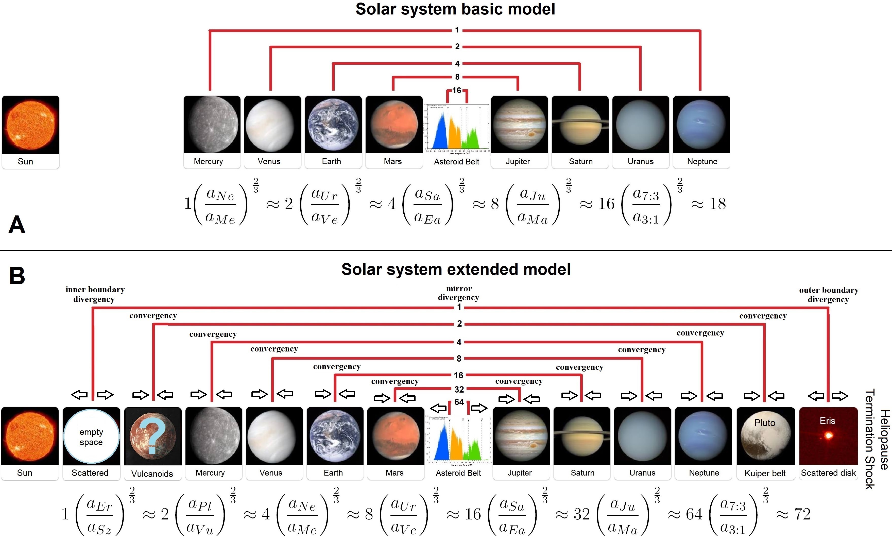
Figure 7: [A] Graphical representation of Eq. 25 expressing the scaling and the mirror symmetries among the semi-major axis lengths of the eight planets of the solar system, including the central region of the asteroid belt, according to the 12-TET model of the Geddes – King-Hele equations (99% accuracy). [B] Graphical representation of the hypothesized scaling and mirror-symmetric planetary organization of the solar system according to the extended model (Eq. 26). The ratio sequences are based on the Pythagorean epogdoon (the interval ratio $9/8=18/16=72/64$) and its addition with up to six octaves.

Eq. 26	$\frac{1}{64}\left(\frac{a_{Er}}{a_{Sz}}\right)^{\frac{2}{3}}$	$\frac{1}{32}\left(\frac{a_{Pl}}{a_{Vu}}\right)^{\frac{2}{3}}$	$\frac{1}{16}\left(\frac{a_{Ne}}{a_{Me}}\right)^{\frac{2}{3}}$	$\frac{1}{8}\left(\frac{a_{Ur}}{a_{Ve}}\right)^{\frac{2}{3}}$	$\frac{1}{4}\left(\frac{a_{Sa}}{a_{Ea}}\right)^{\frac{2}{3}}$	$\frac{1}{2}\left(\frac{a_{Ju}}{a_{Ma}}\right)^{\frac{2}{3}}$	$1\left(\frac{a_{7:3}}{a_{3:1}}\right)^{\frac{2}{3}}$	9/8
val.	1.125 *	1.125 *	1.137	1.113	1.128	1.134	1.118	1.125
acc.	( 100% )	( 100% )	( 101% )	( 99% )	( 100% )	( 101% )	( 99% )

Table 7: Value and accuracy of each element of Eq. 26 obtained with the orbital data in Table 2. ( * Theoretical).

Both Eqs. 25 and 26 can be rewritten as functions of the orbital periods or mean speeds by substituting the exponent 2/3 with 4/9 and 4/3 as in Eqs. 18 and 19, respectively. This transformation does not allow us to interpret the quotients as simple orbital period ratios. Nor does it allow us to do so for orbital frequency relations, which are simply the multiplicative inverses of those derived from orbital periods. The traditional understanding of a gravitational self-organization structure involves some form of linear relation among the orbital frequencies and excludes the application of non-linear transformations. Nevertheless, Eqs. 25 and 26 express relations of pure rational numbers as all quotients are non-dimensional, which is a strong indication of some kind of (still unknown) synchronization phenomena that can emerge from planetary dynamics produced by adding more gravitational bodies and dissipative interactions (tidal forces, radiation pressure, friction, etc.). The question remains on how a non-linear transformation of orbital periods forms these rational ratios, and this represents a challenge from a dynamical point of view that can be addressed in future research. Nevertheless, the robustness of the results is impressive. Once the exponent of the non-linear transformation is optimized at $k=2/3$ (as depicted in Figures 4 and 5), the transformed orbital ratios between neighboring planetary pairs are compatible not only with the tone relations of the traditional 12-TJI and 12-TET musical tuning systems, but also specifically with their consonances. The fact that the error is slightly smaller for just intonation (12-TJI) compared with equal tempered (12-TET) tuning may suggest that the solar system is mostly characterized by super-particular ratios, that is by 3/2, 4/3, 5/4 and 6/5 (including Pluto) used in the former. Moreover, Eqs. 25 and 26 are based on the super-particular ratio 9/8 (Major Second) multiplied by powers of 2. The ratio 9 to 8 was known in Pythagorean music theory as the epogdoon, which corresponds to the whole tone and is derived from the Pythagorean consonances. By extending the mirror-scaling equation (Eq. 26) by two additional rings and noting the planetary contiguous ratios produced, we see that all musical tone relations from the Major Second to the Major Sixth are represented in this model.

The physical interpretation of the result is still based on preliminary planetary models, analogies and speculations.

For example, Pakter and Levin (2018) proposed a planetary model suggesting that, under specific constraints and energy non-conserving perturbations, a planetary system could reach a self-organized periodic state from arbitrary initial conditions. Their model, however, was simplistic and could not properly simulate our solar system. Moreover, no simulation using more than 6 identical planets was stable.

Our proposed empirical planetary model of the solar system is rather peculiar because it suggests a planetary self-organization mechanism that does not directly involve the traditional planetary commensurability models based on whole number ratios of orbital periods, as usually proposed in the literature (cf.: Aschwanden, 2018; Peale, 1976). In fact, the $a^{2/3}$ metric cannot be directly interpreted using the third law of Kepler, Eq. 1, because the latter links the orbital periods to a $a^{3/2}$ metric. Moreover, as demonstrated in section 3, the orbital-period metric does not yield ratios between contiguous planets of our solar system that could be expressed by consonances. Thus, our solar system is not gravitationally self-organized like, for example, the Trappist-1 solar system.

Eqs. 13 may suggest an alternative orbital self-organization process that could involve gravity accelerations, and space and volume ratios instead of the orbital period ones. For example, by assuming that the orbits are circular (so that the semi-major axis coincides with the orbital radius, $a_{1}=R_{1}$ and $a_{2}=R_{2}$), Eq. 7 with $k=2/3$ can be rewritten as:

$$\left(\frac{a_{1}}{a_{2}}\right)^{\frac{2}{3}}=\left(\frac{R_{1}}{R_{2}}\right)^{\frac{2}{3}}=\left(\frac{m_{1}}{m_{2}}\frac{F_{2}}{F_{1}}\right)^{\frac{1}{3}}\approx f$$ (27)

where $m_{1}$ and $m_{2}$ are the masses of the two adjacent planets, and $F_{1}$ and $F_{2}$ are the gravitational forces that attract them toward the Sun ($F=GM_{\odot}m/R^{2}$); for each couple of adjacent planets, the frequencies $f$ assume one of the values $2^{n/12}$ with $n$ = 4, 5, 7 and 8, or, alternatively, $f$ = 5/4, 4/3, 3/2 and 8/5. Thus, our result and Eq. 27 indicate that the cube root of the ratio between the centripetal orbital acceleration of adjacent planets of the solar system can be interpreted as musical tones and, more specifically, as consonances.

A 2/3rd power of an orbital radius could also be interpreted as a geometrical transformation of an ellipsoid of radius $R_{e}$ and fixed height $H$ into an equal volume sphere of radius $R_{s}$ according to the equation $R_{s}=\sqrt[3]{HR^{2}}$. In fact, the solar system is made of a planetary disk and its geometry could be approximated by an ellipsoid with a given height $H$. Thus, each planetary orbit could be associated with an ellipsoid with orbital radius $R$ and a constant height $H$, and could be transformed into a sphere with radius $R^{\prime}=\sqrt[3]{hR^{2}}$. Our results would then imply that the ratios of spherically transformed orbital radii of adjacent planets of the solar system express musical consonances as:

$$\left(\frac{R_{1}}{R_{2}}\right)^{\frac{2}{3}}=\frac{R^{\prime}_{1}}{R^{\prime}_{2}}\approx f.$$ (28)

Table 1 reports the $R^{\prime}$ values for each planet.

We also observe that in physics, equations where cube frequencies appear are not frequent, but one of them is the Planck’s law (or its Wien’s approximation) describing the spectral density of electromagnetic radiation emitted by a black body in thermal equilibrium at a given temperature T (Planck, 1914). Finally, it is interesting to note that the operation needed to obtain the above result from planetary distances – raising them to the 2/3 power – is somehow specular to the operation which relates planetary distances to orbital periods by Kepler’s third law, raising them to the 3/2 power (Eq. 1).

On whether the above or alternative analogies might yield a physical relation between the relatively stable orbits of the solar system and the distribution of gravitational energy in it linked to a 2/3rd power of the orbital radii of the planets, is left to future investigations.

11 Conclusion

An interesting feature of the solar system is its specular-reflection-like architecture which is made of four inner terrestrial planets (Mercury, Venus, Earth and Mars) and four outer gas-giant planets (Jupiter, Saturn, Uranus and Neptune) divided by the asteroid belt. No other exoplanetary system similar to our has been discovered yet.

We have shown the Geddes–King-Hele equations for mirror symmetries among the distances of the planets, when raised to the 2/3rd power, express values that are very close to the simple ratios found in the harmonic consonances of the 12-TET and 12-TJI tuning systems used in Classical and Western music. This result contradicts the brief critique of Abhyankar (1983) that there is “nothing particularly musical” in such equations. Of course, herein, we intend for the word “musical” to relate to the presence of the ratios found in Classical tuning systems which have specific mathematical properties.

Geddes and King-Hele noted the mirror symmetries but not the scaling that we highlighted in our equations. This result further contradicts Abhyankar (1983)’s claim that such equations cannot tell us anything “about the origin of the solar system or its stability”. In fact, it appears that our solar system could be interpreted by Eq. 25 (depicted in Figure 7) or Eq. 26 that relates the ratios of planet pairs mirrored by the asteroid belt as a series weighted by increasing powers of 2 of the Pythagorean tone epogdoon (the 9/8 ratio).

The orbital radii of the inner planets can be predicted from those of the outer ones, and vice versa, with a precision that is about three times superior to that of the harmonic orbit resonance model recently proposed by Aschwanden (2018). In fact, it shows just a 0.8% average error (that is an accuracy larger than 99%) against a 2.5% error of the alternative method. In addition, the probability of finding only musical consonances among such adjacent ratios has a p-value $<0.1$%, which makes it improbable that this is a random result. Furthermore, our model could be extended to predict the inner gap structure of the asteroid belt as well as the transneptunian objects.

Furthermore, Eq. 23 (or Eq. 24) show that the coefficient 18 in Eq. 16 is directly linked to the 3:1 and 7:3 resonances with Jupiter that, by virtue of its large mass, has likely played a decisive role in the orbital architecture of the solar system. This main role seems confirmed in Figure 6A where the planetary predictions of Eq. 13 based on Jupiter (blue curve with circles) are well balanced among the other series. The two cited resonances characterize the main Kirkwood gaps of the asteroid belt. Thus, although the physics behind such a result is not determined yet, these empirical relations do not appear to be coincidental.

We also determined that for exponents $k$ close to $2/3$ there is a convergent minimum both in the average and maximum error between our proposed planetary metric and both the 12 musical tones and the 7 harmonic consonances. More specifically, for the solar system, such planetary ratios are represented by harmonic musical consonances that assume frequency values equal to $2^{n/12}$ with $n$ = 4, 5, 7 and 8, or, alternatively, 5/4 (Major Third), 4/3 (Perfect Fourth), 3/2 (Perfect Fifth) and 8/5 (Minor Sixth). Interestingly, the seven planets of the Trappist-1 solar system (labeled b, c, d, e, f, g and h) present a set of approximate orbital resonance ratios in the periods of adjacent planets (from b$\leftrightarrow$c to g$\leftrightarrow$h) that includes the same consonances: these are 8:5, 5:3, 3:2, 3:2, 4:3, 3:2 (cf. Agol et al., 2021; Gillon et al., 2017; Tamayo et al., 2017), which correspond to the tones $Ab$, $A$, $G$, $G$, $F$ and $G$ (with C as a reference tone). Thus, we suggest that quasi-stable orbital systems could be characterized by standard whole number ratios as those that characterize the musical consonances. However, these ratios can involve physical observables other than the orbital periods. Therefore, alternative and/or complementary orbital metrics should be considered for describing orbital systems.

In fact, mean motion resonances, in which the orbital periods or mean angular velocities of planetary bodies are in ratios of small integers, are commonplace in planetary systems, both in our own solar system and in exoplanetary systems. The Trappist system that we mention is a good example, while in our own solar system, a whole network of mean motion resonances exist among the inner satellites of Saturn, for example, with many other examples existing elsewhere (e.g. Aschwanden, 2018). These relationships are today well-understood as they satisfy Kepler’s third law and can be easily explained within the context of the laws of planetary motion based on Newtonian gravity. The physical mechanisms underpinning them, together with the secular and tidal evolution processes which bring them about are well-established, and astrophysicists have a good understanding of the interplay between regular and chaotic motion which is fundamental to these (and actually to some degree all) dynamical systems. However, such findings do not exclude the possibility of alternative physical forms of self-organization of orbital systems which are today still unknown or have not yet been investigated.

For our solar system, the consonant ratios among adjacent planets emerge when the ellipsoid orbital radii are transformed into equal-volume spherical radii using the exponent $k=2/3$, but for the Trappist-1 system, the orbital radii are to be transformed into periods using the exponent $k=3/2$. Thus, it appears that what happens for the solar system cannot be easily explained in terms of the usual Newtonian motion resonance approaches. The evidence suggests that the exponent $k$ could differ for different orbital systems and the found $k=2/3$ exponent may express an alternative metric capable of producing a self-organizing orbital structure.

These different kinds of harmonic structures could in the future be properly understood and classified as more and more exoplanetary systems are discovered. This task is made more difficult today because testing for a relationship such as Eq. 25 in exoplanetary systems may not be possible until our knowledge of them is complete. In fact, it is difficult to fully characterize detailed orbital information for all the large and small planets, in addition to possible asteroid belts in distant exoplanetary systems. The challenge for future research would be to justify the proposed metric on physical grounds or to find a better physical explanation for the self-organization of the solar system, which, however, is today a matter of debate.

In conclusion, the ratios of the orbital radii of adjacent planets of our solar system, when raised to the 2/3rd power, express the simple ratios found in harmonic musical consonances and can be expressed by a simple, elegant, and highly precise equation that reveals scaling and mirror-like symmetries of its planetary orbital distribution relative to the asteroid belt, whose inner structure is also predicted by the same model depicted in Figure 7. Eqs. 25 and 26 suggest that the orbital scaling-mirror symmetries of the solar system could be expressed by the Pythagorean epogdoon (the tone ratio 9/8) and its addition with up to six octaves. Furthermore, the ratio 9/8 is closely related to the 3:1 and 7:3 resonances of Jupiter that shape the asteroid belt (Eq. 24), which indicates the primary role played by Jupiter in organizing the planetary orbits of the solar system.

The mathematical correlation which we presented between idealized musical ratios and planetary data is very similar to what Johannes Kepler was seeking when he published his Harmonices Mundi in 1619. Our result further indicates that the orbital movements of the major bodies of the solar system are likely highly organized. In this regard, we would also like to point out that aesthetic perception of patterns in our surroundings is a fundamental dimension of the human culture, and it has been crucial in the development of a scientific understanding of the natural world. Thus, our empirical model could lead to the future discovery of important dynamical structures of orbital systems, which today are still unknown. The final paragraph of Geddes & King-Hele’s original 1983 paper is worth quoting:

“The significance of the many near-equalities is very difficult to assess. The hard-boiled may dismiss them as mere playing with numbers; but those with eyes to see and ears to hear may find traces of ‘something far more deeply interfused’ in the fact that the average interval between the musical notes emerges as the only numerical constant required - a result that would surely have pleased Kepler.”

Appendix

Eq. 26 can be rewritten also in the following forms that highlight better how each pairs of planets is directly linked to the Pythagorean epogdoon ratio 9/8 (or 8/9):

$$\frac{1}{64}\left(\frac{a_{Er}}{a_{Sz}}\right)^{\frac{2}{3}}\approx\frac{1}{32}\left(\frac{a_{Pl}}{a_{Vu}}\right)^{\frac{2}{3}}\approx\frac{1}{16}\left(\frac{a_{Ne}}{a_{Me}}\right)^{\frac{2}{3}}\approx\frac{1}{8}\left(\frac{a_{Ur}}{a_{Ve}}\right)^{\frac{2}{3}}\approx\frac{1}{4}\left(\frac{a_{Sa}}{a_{Ea}}\right)^{\frac{2}{3}}\approx\frac{1}{2}\left(\frac{a_{Ju}}{a_{Ma}}\right)^{\frac{2}{3}}\approx 1\left(\frac{a_{7:3}}{a_{3:1}}\right)^{\frac{2}{3}}\approx\frac{9}{8}$$ (29)

$$64\left(\frac{a_{Sz}}{a_{Er}}\right)^{\frac{2}{3}}\approx 32\left(\frac{a_{Vu}}{a_{Pl}}\right)^{\frac{2}{3}}\approx 16\left(\frac{a_{Me}}{a_{Ne}}\right)^{\frac{2}{3}}\approx 8\left(\frac{a_{Ve}}{a_{Ur}}\right)^{\frac{2}{3}}\approx 4\left(\frac{a_{Ea}}{a_{Sa}}\right)^{\frac{2}{3}}\approx 2\left(\frac{a_{Ma}}{a_{Ju}}\right)^{\frac{2}{3}}\approx 1\left(\frac{a_{3:1}}{a_{7:3}}\right)^{\frac{2}{3}}\approx\frac{8}{9}$$ (30)

Data availability

The calculations presented herein are based on the orbital data listed in Table 2 which are provided by NASA: https://nssdc.gsfc.nasa.gov/planetary/factsheet/

Contributions

MB contributed to the interpretation of the results based on music theory; NS developed the scientific and astronomical interpretation of the results, wrote and organized the paper. Both authors share first authorship, contributed to the discussion and have read and edited the text of the final manuscript.

Competing interests

The authors declare that the research was conducted in the absence of any commercial or financial relationships that could be construed as a potential conflict of interest.

References

- Abhyankar (1983) Abhyankar, K.D. (1983). Music of the spheres. The Observatory 103, 260–260.
- Agol et al. (2021) Agol, E., Dorn, C., Grimm, S.L., et al. (2021). Refining the Transit-timing and Photometric Analysis of TRAPPIST-1: Masses, Radii, Densities, Dynamics, and Ephemerides. Planetary Science Journal 2, 1.
- Aschwanden (2018) Aschwanden, M.J. (2018). Self-organizing systems in planetary physics: Harmonic resonances of planet and moon orbits. New Astronomy 58, 107–123.
- Basano and Hughes (1979) Basano, L., Hughes, D.W. (1979). A modified Titius-Bode law for planetary orbits. Il Nuovo Cimento C 2, 505–510.
- Beer et al. (2018) Beer, J., Tobias, S.M., Weiss, N.O. (2018). On long-term modulation of the Sun’s magnetic cycle. Monthly Notices of the Royal Astronomical Society 473, 1596–1602.
- Bode (1772) Bode, J. E. Anleitung zur Kenntnis des gestirten Himmels, (2nd Edn., Hamburg, 1772).
- Bones et al. (2014) Bones, O., Hopkins, K., Krishnan, A., Plack, C.J. (2014). Phase locked neural activity in the human brainstem predicts preference for musical consonance. Neuropsychologia 58, 23–32.
- Cartwright et al. (2021) Cartwright, J.H.E., González, D.L., Piro, O. (2021). Dynamical Systems, Celestial Mechanics, and Music: Pythagoras Revisited. Math Intelligencer 43, 25–39.
- Chang (2017) Chang, K. The Harmony That Keeps Trappist-1’s 7 Earth-size Worlds From Colliding. (The New York Times, 10 May 2017. Retrieved 4 May, 2021).
- Charvatova (1997) Charvàtovà, I. (1997). Solar-terrestrial and climatic phenomena in relation to solar inertial motion. Surveys in Geophysics 18, 131–146.
- Evans et al. (1999) Evans, N. W, Tabachnik, S. (1999). Possible long-lived asteroid belts in the inner solar system. Nature 399, 41–43.
- Forster (2010) Forster, C. Musical Mathematics: On the Art and Science of Acoustic Instruments. (Chronicle Books, 2010).