Distribution Regression with Sliced Wasserstein Kernels

Abstract

The problem of learning functions over spaces of probabilities – or distribution regression – is gaining significant interest in the machine learning community. A key challenge behind this problem is to identify a suitable representation capturing all relevant properties of the underlying functional mapping. A principled approach to distribution regression is provided by kernel mean embeddings, which lifts kernel-induced similarity on the input domain at the probability level. This strategy effectively tackles the two-stage sampling nature of the problem, enabling one to derive estimators with strong statistical guarantees, such as universal consistency and excess risk bounds. However, kernel mean embeddings implicitly hinge on the maximum mean discrepancy (MMD), a metric on probabilities, which may fail to capture key geometrical relations between distributions. In contrast, optimal transport (OT) metrics, are potentially more appealing. In this work, we propose an OT-based estimator for distribution regression. We build on the Sliced Wasserstein distance to obtain an OT-based representation. We study the theoretical properties of a kernel ridge regression estimator based on such representation, for which we prove universal consistency and excess risk bounds. Preliminary experiments complement our theoretical findings by showing the effectiveness of the proposed approach and compare it with MMD-based estimators.

1 Introduction

Distribution regression studies the problem of learning a real-valued function defined on the space of probability distributions from a sequence of input/output observations. A peculiar feature of this setting is that, typically, the input distributions are not observed directly but only accessed through finite samples, adding complexity to the problem (Póczos et al., 2013). A typical example in the literature (see Szabó et al., 2016; Fang et al., 2020) is the task of predicting some health indicator of patients, labeled by $t$, based on their distribution $\mathbb{P}_{t}$ over results of clinical investigations, e.g. blood measurements. The underlying distribution of test results for each patient is observed only through repeated medical tests $x_{t,i}\sim\mathbb{P}_{t}$, $i=1,\ldots,n_{t}$, forming an approximation of $\mathbb{P}_{t}$ through $\hat{\mathbb{P}}_{t,n_{t}}=\frac{1}{n_{t}}\sum_{i=1}^{n_{t}}\delta_{x_{i}}$. Given labeled examples $(\hat{\mathbb{P}}_{t,n_{t}},y_{t})_{t=1}^{T}$, where $y_{t}$ is the health indicator, we seek to learn an accurate mapping $f:\hat{\mathbb{P}}_{n}\to y$ for a new patient identified by $\mathbb{P}$. Other examples of interest for the machine learning community include the task of predicting summary statistics of distributions such as the entropy or the number of modes (Oliva et al., 2014) or for conditional meta-learning (Denevi et al., 2020).

Historically, distribution regression has been tackled by means of a two-stage procedure, that build upon the kernel mean embedding machinery (Smola et al., 2007; Muandet et al., 2017). A first positive definite (p.d.) kernel (Smola & Schölkopf, 1998) defined on the underlying data space is used to embed the distribution $\hat{\mathbb{P}}_{t,n_{t}}$ into an Hilbert space, and then a second kernel is used as a similarity measure between the embedded distributions to perform Kernel Ridge Regression (KRR). This approach has been theoretically investigated in Szabó et al. (2016) and further analyzed in Fang et al. (2020). More recently, a SGD variant (Mücke, 2021) and a robust variant (Yu et al., 2021) have been suggested.

The two stages above allow to build a p.d. kernel on the space of probability distributions and provide an example of distance substitution kernel, a class of kernels that can be built from distances on metric spaces (Haasdonk & Bahlmann, 2004). In that particular setting the chosen distance is the Maximum Mean Discrepancy (MMD), a metric on probability distributions (Gretton et al., 2012). A main theme of this paper is that distance substitution kernels based on optimal transport (with the Wasserstein distance) might be preferable over MMD-based ones, as they may better capture the geometry of the space of distributions (Peyré et al., 2019).

The above observations lead us to introduce a Wasserstein-based p.d. kernel for distribution regression. As the original Wasserstein distance cannot be used to build a p.d. kernel on the space of distributions our construction exploits the Sliced-Wasserstein (SW) distance (Bonneel et al., 2015), a computationally cheapest alternative to the standard Wasserstein distance. SW is raising significant interest in the machine learning community due to its attractive topological and statistical properties (Nadjahi et al., 2019, 2020; Nadjahi, 2021) and its strong numerical performances (Kolouri et al., 2018, 2019; Deshpande et al., 2018, 2019; Lee et al., 2019) and references therein.

A SW-based kernel was first introduced in Kolouri et al. (2016), but their construction was restricted to the subset of absolutely continuous distributions. Hence, this approach is not suitable for the distribution regression problem where we need to handle empirical distributions of the form $\hat{\mathbb{P}}_{t,n}$. In parallel, a SW-based kernel has been developed for persistence diagrams in topological data analysis Carriere et al. (2017). Bachoc et al. (2017); Trang et al. (2021) defined a p.d. kernel based on the Wasserstein distance valid for any probability measure defined on $\mathbb{R}$; while Bachoc et al. (2020) used a similar extension to ours to $\mathbb{R}^{r}$, $r\geq 1$ focusing on Gaussian process distribution regression. In this paper however, we focus on statistical properties of the estimator within a kernel method setting.

Finally, there are deep learning heuristic methods to tackle the problem of learning from distributions such as deep sets Zaheer et al. (2017) and references therein. While they might perform well in practice, they are harder to analyse theoretically and fall outside the scope of kernel methods which is the focus of this present work.

Contributions.   This paper provides four main contributions: 1) we present a Wasserstein-based p.d. kernel valid for any probability distribution on $\mathbb{R}^{r}$; 2) we show that such kernel is universal in the sense of Christmann & Steinwart (2010), allowing us to asymptotically learn any distribution regression function; 3) we provide excess risk bounds for the KRR estimator based on such kernels, which implies its consistency; 4) finally, we provide empirical evidences that the SW kernels behave better than MMD kernels on a number of distribution regression tasks.

Paper organisation.   The rest of the paper is organized as follows: Sec. 2 introduces the distribution regression setting and Sec. 3 reviews distance substitution kernels as a way to approach such problems. Sec. 4 shows that the SW distance can be used to obtain universal distance substitution kernels. Sec. 5 characterizes the generalization properties of distribution regression estimators based on distance substitution kernels. Sec. 6 reports empirical evidences supporting the adoption of SW kernels in practical applications.

2 Distribution regression

Tools and notations.  By convention, vectors $v\in\mathbb{R}^{r}$ are seen as $r\times 1$ matrices and $\|v\|$ denotes their Euclidean norm. $A^{\top}$ denotes the transpose of any $r\times k$ matrix $A$, $I_{r}\in\mathbb{R}^{r\times r}$ the identity matrix and $I$ the identity operator. For a measurable space $(\Omega,\mathcal{A})$ we denote by $\mathcal{M}_{+}^{1}(\Omega)$ the space of probability measures on $(\Omega,\mathcal{A})$. Throughout most of the paper we use $\mathcal{M}_{+}^{1}(\Omega_{r})$ with $\Omega_{r}$ a compact subset of $\mathbb{R}^{r}$. For two measurable spaces $(\Omega,\mathcal{A}),(\mathcal{X},\mathcal{B})$ and a measurable map $T:\Omega\to\mathcal{X}$, the push-forward operator $T_{\#}:\mathcal{M}_{+}^{1}(\Omega)\to\mathcal{M}_{+}^{1}(\mathcal{X})$ is defined such that for all $\alpha\in\mathcal{M}_{+}^{1}(\Omega)$ and for all measurable set $B\in\mathcal{B}$, $T_{\#}(\alpha)(B)=\alpha(T^{-1}(B))$. $S^{r-1}=\{x\in\mathbb{R}^{r}\mid\|x\|_{2}=1\}$ denotes the unit sphere in $\mathbb{R}^{r}$. $\lambda^{r}$ is the Lebesgue measure on $\mathbb{R}^{r}$ and $\sigma^{r}$ is the uniform probability measure on the unit sphere, we use $dx$ instead of $\lambda^{r}(dx)$ and $d\theta$ instead of $\sigma^{r}(d\theta)$ when there is no ambiguity. For a vector $\theta\in S^{r-1}$, $\theta^{*}:\mathbb{R}^{r}\to\mathbb{R},x\mapsto\langle x,\theta\rangle$. For a univariate probability measure $\alpha\in\mathcal{M}_{+}^{1}(\mathbb{R})$, we denote by $F_{\alpha}$ its cumulative distribution function, $F_{\alpha}(x)=\alpha((-\infty,x])\in[0,1]$, by $F_{\alpha}^{[-1]}$ its generalised inverse cumulative distribution function, $F_{\alpha}^{[-1]}(x)=\inf\{t\in\mathbb{R}:F_{\alpha}(t)\geq x\}$, and by $F_{\alpha}^{-1}$ its inverse cumulative distribution function, if it exists. On a measure space $(\Omega,\mathcal{A},\mu)$ we denote by $L^{2}(\Omega,\mu)$, abbreviated $L^{2}_{\mu}$ if the context is clear, the Hilbert space of square-integrable functions with respect to $\mu$ from $\Omega$ to $\mathbb{R}$ with norm $\|\cdot\|_{L^{2}_{\mu}}$ induced by the inner product $\langle f,g\rangle_{L^{2}_{\mu}}=\int_{\Omega}f(w)g(w)d\mu(w)$. Finally, for a compact set $\Omega$, $\mathcal{U}(\Omega)$ denotes the uniform distribution on $\Omega$.

Problem set-up.  Linear regression considers Euclidean vectors as covariate while kernel regression extends the framework to any covariate space $X$ on which we can define a p.d. kernel $K:X\times X\to\mathbb{R}$ (Hofmann et al., 2008). In distribution regression, $X$ is a space of probability measures with the additional difficulty that the covariates $\mathbb{P}\in X$ cannot be directly observed (Póczos et al., 2013). Each $\mathbb{P}\in X$ is only accessed through i.i.d. samples $\{x_{i}\}_{i=1}^{n}\sim\mathbb{P}$, which forms a noisy measurement of $\mathbb{P}$. The formal problem set up is as follows. $X:=\mathcal{M}_{+}^{1}(\Omega_{r})$ is a space of probability distributions, we refer to $X$ as the input space and $\Omega_{r}$ as the (compact) data space. $Y\subseteq\mathbb{R}$ is a real subset and $\rho$ is an unknown distribution on $Z:=X\times Y$. $\rho_{X}$ is its marginal distribution on $X$ and $\rho_{Y\mid X}$ is its conditional distribution: $\rho(\mathbb{P},y)=\rho_{Y\mid X}(y\mid\mathbb{P})\rho_{X}(\mathbb{P})$. The goal is to find a measurable map $f:X\to Y$ with low expected risk

$$\mathcal{E}(f)=\int_{Z}(f(\mathbb{P})-y)^{2}d\rho(\mathbb{P},y).$$ (1)

The minimizer of this functional (see Prop. 11) is the regression function

$$f_{\rho}(\mathbb{P})=\int_{Y}yd\rho_{Y\mid X}(y\mid\mathbb{P}),\qquad\forall~{}\mathbb{P}\in X,$$ (2)

which is not accessible since $\rho$ is unknown. To approximate $f_{\rho}$ we draw a set of input-label pairs $\mathcal{D}=(\mathbb{P}_{t},y_{t})_{t=1}^{T}\sim^{i.i.d}\rho$. We call this the first stage sampling. If we were in a standard regression setting, i.e. the inputs $\mathbb{P}_{t}$ were directly observable, given a p.d. kernel $K$ on $X$, one approach would be to apply KRR by minimizing the regularized empirical risk:

$$\mathcal{E}_{T,\lambda}(f)=\frac{1}{T}\sum_{t=1}^{T}\left(f\left(\mathbb{P}_{t}\right)-y_{t}\right)^{2}+\lambda\|f\|_{\mathcal{H}_{K}}^{2}$$ (3)

where $\mathcal{H}_{K}$ is te Reproducing Kernel Hilbert Space (RKHS) induced by $K$. We refer to this quantity as the first stage empirical risk and denote its minimizer $f_{\mathcal{D},\lambda}$. The difference with standard regression comes from the second stage of sampling were instead of directly observing the covariates we receive for each input a bag of samples: $\hat{\mathcal{D}}=\{((x_{t,i})_{i=1}^{n},y_{t})\}_{t=1}^{T}$, $(x_{t,i})_{i=1}^{n}\sim^{i.i.d}\mathbb{P}_{t}$. For ease of notations, we assume without loss of generality that each bag has the same number of points $n$. The strategy is then to plug the empirical distributions $\hat{\mathbb{P}}_{t,n}=\frac{1}{n}\sum_{i=1}^{n}\delta_{x_{t,i}}$ in the first stage risk leading to the second stage risk:

$$\mathcal{E}_{T,n,\lambda}(f)=\frac{1}{T}\sum_{t=1}^{T}\left(f\left(\hat{\mathbb{P}}_{t,n}\right)-y_{t}\right)^{2}+\lambda\|f\|_{\mathcal{H}_{K}}^{2}.$$ (4)

We denote by $f_{\hat{\mathcal{D}},\lambda}$ its minimizer.

Kernel distribution regression.  Equipped with a p.d. kernel $K:X\times X\to\mathbb{R}$, minimizing $\mathcal{E}_{T,n,\lambda}$ over $\mathcal{H}_{K}$ leads to a practical algorithm. For a new test point $\mathbb{P}\in X$,

$$f_{\hat{\mathcal{D}},\lambda}(\mathbb{P})=(y_{1},\ldots,y_{T})(K_{T}+\lambda TI_{T})^{-1}k_{\mathbb{P}}$$ (5)

where $[K_{T}]_{t,l}=K(\hat{\mathbb{P}}_{t,n},\hat{\mathbb{P}}_{l,n})\in\mathbb{R}^{T\times T}$ and
$k_{\mathbb{P}}=(K(\mathbb{P},\hat{\mathbb{P}}_{t,n}),\ldots,K(\mathbb{P},\hat{\mathbb{P}}_{T,n}))^{\top}\in\mathbb{R}^{T}$ (see Prop. 12). Let us note that in practice the new test points will also have the form of empirical distributions $\hat{\mathbb{P}}_{n}=\frac{1}{n}\sum_{i=1}^{n}\delta_{x_{i}}$. The algorithm will differ by which kernel is used on $X$.

3 Distance substitution kernels

In this section, we derive two types of kernels that can be defined on $X$. We approach this through the prism of distance substitution kernels. Let us assume that we have a set $M$ on which we want to define a p.d. kernel and we are given a pseudo-distance $d$ on $M$. Pseudo means that $d$ might not satisfy $d(x,y)=0\implies x=y$ for all $(x,y)\in M^{2}$. One could think of using $d$ to define a p.d kernel on $M$ by substituting $d$ to the Euclidean distance for usual Euclidean kernels (Haasdonk & Bahlmann, 2004). For example,

$$K_{\rm Gauss}(x,y)=e^{-\gamma d(x,y)^{2}},$$ (6)

(with $x,y\in M$) generalizes the well-known Gaussian kernel $K_{\rm Gauss}(x,y)=e^{-\gamma\|x-y\|^{2}}$ (with $x,y\in\mathbb{R}^{r}$). Analogously, given an origin point $x_{0}\in M$, the kernel

$$\langle x,y\rangle_{d}^{x_{0}}:=\frac{1}{2}\Big{(}d(x,x_{0})^{2}+d(y,x_{0})^{2}-d(x,y)^{2}\Big{)},$$ (7)

generalizes the linear kernel (with origin in $0$)

$$\langle x,y\rangle=\frac{1}{2}\Big{(}\|x\|^{2}+\|y\|^{2}-\|x-y\|^{2}\Big{)}.$$ (8)

However, this type of substitution does not always lead to a valid kernel. In fact, the class of distances such that $K_{\rm Gauss}$ and $\langle\cdot,\cdot\rangle_{d}^{x_{0}}$ are p.d. is completely characterised by the notion of Hilbertian (pseudo-)distance (Hein & Bousquet, 2005). A pseudo-distance $d$ is said to be Hilbertian if there exists a Hilbert space $\mathcal{F}$ and a feature map $\Phi:\mathcal{X}\to\mathcal{F}$ such that $d(x,y)=||\Phi(x)-\Phi(y)||_{\mathcal{F}}$ for all $x,y\in M$. The functions $K_{\rm Gauss}$ and $\langle\cdot,\cdot\rangle_{d}^{x_{0}}$ are p.d. kernels if and only if the corresponding $d$ is Hilbertian. We refer to such kernels as distance substitution kernels and we denote them as $K(d)$ (Proposition 13 in the Appendix provides more details on distance substitution kernels).

Remark 1.

An Hilbertian pseudo-distance $d$ is a proper distance if and only if $\Phi$ is injective.

Remark 2.

For an Hilbertian distance $d$, $\langle x,y\rangle_{d}^{x_{0}}=\langle\Phi(x)-\Phi(x_{0}),\Phi(y)-\Phi(x_{0})\rangle_{\mathcal{F}}$.

Hence defining p.d. kernels on $M=X$ boils down to find Hilbertian distances on $X$. Below we give two examples of such distances.

MMD-based kernel.  For a bounded kernel $K_{\Omega}$ defined on the data space $\Omega_{r}$ and its RKHS $\mathcal{H}_{\Omega}$, the Maximum Mean Discrepancy (MMD) pseudo-distance is for all $(\mathbb{P},\mathbb{Q})\in X^{2}$

$$d_{\rm MMD}(\mathbb{P},\mathbb{Q})=\|\mu_{K_{\Omega}}(\mathbb{P})-\mu_{K_{\Omega}}(\mathbb{Q}))\|_{\mathcal{H}_{\Omega}},$$ (9)

where $\mu_{K_{\Omega}}:\mathbb{P}\mapsto\int_{\Omega_{r}}K_{\Omega}(x,\cdot)d\mathbb{P}(x)\in\mathcal{H}_{\Omega}$ is the kernel mean embedding operator (Berlinet & Thomas-Agnan, 2011). $d_{\rm MMD}$ is by construction Hilbertian with $\mathcal{F}=\mathcal{H}_{\Omega}$ and $\Phi=\mu_{K_{\Omega}}$. Note that using MMD to build a kernel on $X$ requires two kernels, a kernel on $\Omega_{r}$ to build $d_{\rm MMD}$ and the outer kernel $K(d_{\rm MMD})$. Previous theoretical studies of distribution regression focused exclusively on MMD-based kernels (Szabó et al., 2016; Fang et al., 2020). We will show that the established theory for MMD-based distribution regression can be extended to a larger class of distance substitution kernels.

Remark 3.

$d_{\rm MMD}$ is a proper distance if and only if $K_{\Omega}$ is characteristic, i.e. $\mu_{K_{\Omega}}$ is injective.

Fourier Kernel.  Let $\mathbb{P}\in X$, its Fourier transform $F\left(\mathbb{P}\right)$ is defined by $F\left(\mathbb{P}\right)(t)=\int e^{i\langle x,t\rangle}d\mathbb{P}(x)$, $t\in\mathbb{R}^{r}$. In Christmann & Steinwart (2010) the distance

$$d_{F}(\mathbb{P},\mathbb{Q})=\|F\left(\mathbb{P}\right)-F\left(\mathbb{Q}\right)\|_{L^{2}_{\mu}}$$ (10)

was considered, where $\mu$ is a finite Borel measure with support over $\mathbb{R}^{r}$. $d_{F}$ is clearly Hilbertian and is a proper distance since the Fourier transform is injective.

Universality of Gaussian-like kernels.  Kernels of the form 6 with both the MMD and the Fourier distances can be shown to be universal for $X$ equipped with the topology of the weak convergence in probability.

Definition 1.

A continuous kernel $K$ on a compact metric space $(\mathcal{X},d_{\mathcal{X}})$ is called universal if the RKHS $\mathcal{H}_{K}$ of $K$ is dense in $C(\mathcal{X},d_{\mathcal{X}})$, i.e. for every function $g:\mathcal{X}\to\mathbb{R}$ continuous with respect to $d_{\mathcal{X}}$ and all $\varepsilon>0$ there exists an $f\in\mathcal{H}_{K}$ such that $\|f-g\|_{\infty}:=\sup_{x\in X}|f(x)-g(x)|\leq\varepsilon$.

Universality is an important property that indicates when a RKHS is powerful enough to approximate any continuous function with arbitrarily precision. We recall here a fundamental result regarding universality that we will use in the next section.

Theorem 4 (Christmann & Steinwart (2010), Theorem 2.2).

On a compact metric space $(\mathcal{X},d_{\mathcal{X}})$ and for a continuous and injective map $\Phi:\mathcal{X}\to\mathcal{F}$ where $\mathcal{F}$ is a separable Hilbert space, $K(x,y)=e^{-\gamma\|\Phi(x)-\Phi(x^{\prime})\|_{\mathcal{F}}^{2}}$ is universal.

For $\mathcal{X}=X$ and $d_{P}$ the Prokhorov distance, which induced the topology describing the weak convergence of probability measures, Christmann & Steinwart (2010) uses this result to show that MMD (when the inner kernel is characteristic) and Fourier based Gaussian-like kernels are universal.

4 Sliced Wasserstein Kernels

We introduce the tools needed to define the Sliced Wasserstein kernels and give the first proof that SW Gaussian-like kernels are universal. Arising from the field of optimal transport (Villani, 2009), the Wasserstein metric is a natural distance to compare probability distributions.

Wasserstein distance.  For $p\geq 1$, the $p-$Wasserstein distance on $X=\mathcal{M}_{+}^{1}(\Omega_{r})$ is

$$d_{W_{p}}(\mathbb{P},\mathbb{Q})^{p}:=\inf_{\pi\in\mathcal{U}(\mathbb{P},\mathbb{Q})}\int_{\mathbb{R}^{r}\times\mathbb{R}^{r}}\|x-y\|^{p}_{2}\mathrm{d}\pi(x,y),$$ (11)

where $\mathcal{U}(\mathbb{P},\mathbb{Q}):=\{\pi\in X\otimes X\mid P^{1}_{\#}\pi=\mathbb{P},P^{2}_{\#}\pi=\mathbb{Q}\}$ and $P^{i}:\mathbb{R}^{r}\times\mathbb{R}^{r}\to\mathbb{R}^{r},(x_{1},x_{2})\mapsto x_{i}$, $i=1,2$.

One dimensional optimal transport.  The Wasserstein distance usually cannot be computed in closed form. For empirical distributions, it requires to solve a linear program that becomes significantly expensive in high-dimension. However, when $r=1$, the following closed form expression holds (Santambrogio, 2015, Proposition 2.17)

$$d_{W_{p}}(\mathbb{P},\mathbb{Q})=\|F_{\mathbb{P}}^{[-1]}-F_{\mathbb{Q}}^{[-1]}\|_{L^{p}(0,1)},$$ (12)

where $L^{p}(0,1)$ if the set of $p-$integrable functions w.r.t the Lebesgue measure on $(0,1)$. If $\mathbb{P}$ and $\mathbb{Q}$ are empirical distributions, this can be handily computed by sorting the points and computing the average distance between the sorted samples; see Appendix D for more details. In what follows, we will either consider $p=1$ or $p=2$.

Sliced Wasserstein distance.  The closed-form expression of the one-dimensional Wasserstein distance can be lifted to $r>1$ using the mechanism of sliced divergences Nadjahi et al. (2020). The Sliced Wasserstein (SW) distance is defined as,

$$d_{{\rm SW}_{p}}(\mathbb{P},\mathbb{Q})^{p}=\int_{\mathbb{S}^{r-1}}d_{W_{p}}{\left(\theta^{*}_{\#}\mathbb{P},\theta^{*}_{\#}\mathbb{Q}\right)}^{p}d\theta.$$ (13)

The distance averages the one-dimensional distances by projecting the data in every direction $\theta\in\mathbb{S}^{r-1}$. In practice, the integral over $S^{r-1}$ is approximated by sampling directions uniformly, see Appendix D. $d_{{\rm SW}_{p}}$ was introduced in Bonneel et al. (2015) in the context of Wasserstein barycenters and has been heavily used since as a computationally cheaper alternative to the Wasserstein distance. In addition to keeping a closed form expression, $d_{{\rm SW}_{p}}$ inherits useful topological properties from $d_{{\rm W}_{p}}$: it defines a distance on $\mathcal{M}_{+}^{1}(\Omega_{r})$ that implies the weak convergence of probability measures (Nadjahi et al., 2019, 2020). More importantly, $d_{{\rm SW}_{1}}$ and $d_{{\rm SW}_{2}}$ can be used to build a p.d. kernel on $\mathcal{M}_{+}^{1}(\Omega_{r})$, while it would not be possible with the original Wasserstein distance as the induced Wasserstein space has curvature Feragen et al. (2015). Indeed, we now show that $\sqrt{d_{{\rm SW}_{1}}}$ and $d_{{\rm SW}_{2}}$ are Hilbertian distances. Leveraging on the observations in Sec. 3 we conclude that $e^{-\gamma{\rm SW}_{2}^{2}(\cdot,\cdot)}$ and $e^{-\gamma{\rm SW}_{1}(\cdot,\cdot)}$ are valid kernels on probability measures.

${\rm SW}_{2}$-kernel.  To show that $d_{{\rm SW}_{2}}$ is Hilbertian we build an explicit feature map and feature space.

Proposition 5.

$d_{{\rm SW}_{2}}$ is Hilbertian.

Proof.

Taking $\mathcal{F}=L^{2}\left((0,1)\times S^{r-1},\lambda^{1}\otimes\sigma^{r}\right)$ and

$$\Phi:X\to\mathcal{F},\mathbb{P}\mapsto\left((t,\theta)\mapsto F_{\theta^{*}_{\#}\mathbb{P}}^{[-1]}(t)\right),$$ (14)

we have,

$$d_{{\rm SW}_{2}}(\mathbb{P},\mathbb{Q})^{2} =\int_{S^{r-1}}\left\|F_{\theta^{*}_{\#}\mathbb{P}}^{[-1]}-F_{\theta^{*}_{\#}\mathbb{Q}}^{[-1]}\right\|_{L^{2}([0,1])}^{2}d\theta$$

$$=\int_{S^{r-1}}\int_{0}^{1}\left(F_{\theta^{*}_{\#}\mathbb{P}}^{[-1]}(t)-F_{\theta^{*}_{\#}\mathbb{Q}}^{[-1]}(t)\right)^{2}dtd\theta$$

$$=\|\Phi(\mathbb{P})-\Phi(\mathbb{Q})\|_{\mathcal{F}}^{2},$$

as desired. ∎

Note that since we already know that $d_{{\rm SW}_{2}}$ is a proper distance, it implies that $\Phi$ is injective.

Comparison with Kolouri et al. (2016).  Distance substitution kernels with $d_{{\rm SW}_{2}}$ were originally proposed in Kolouri et al. (2016) where it was first shown that such distance is Hilbertian. However, these results were limited to probability distributions admitting a density with respect to the Lebesgue measure. This was due to a different choice of feature map $\Phi$ in the proof of Prop. 5 based on the Radon transform. In dimension one, when a probability $\mathbb{P}\in\mathcal{M}_{+}^{1}(\Omega_{1})$ admits a density $f=\frac{d\mathbb{P}}{d\lambda^{1}}$, the $2-$Wasserstein distance is

$$d_{W_{2}}(\mathbb{P},\mathbb{Q})^{2}=\int_{\mathbb{R}}(F_{\mathbb{Q}}^{[-1]}\circ F_{\mathbb{P}}(t)-t)^{2}f(t)dt.$$

If $\mathbb{P}\in\mathcal{M}_{+}^{1}(\Omega_{r})$ admits a density, then for any direction $\theta\in\mathbb{S}^{r-1}$, $\theta^{*}_{\#}\mathbb{P}$ admits as density $\mathcal{R}f(.,\theta)$ on $\mathbb{R}$, with $\mathcal{R}$ the Radon transform. Then the SW distance is,

$$d_{{\rm SW}_{2}}(\mathbb{P},\mathbb{Q})^{2}=\int(F_{\theta^{*}_{\#}\mathbb{Q}}^{[-1]}\circ F_{\theta^{*}_{\#}\mathbb{P}}(t)-t)^{2}\mathcal{R}f(t,\theta)dtd\theta,$$

Showing that $d_{{\rm SW}_{2}}$ is Hilbertian using the above characterization is less direct than our approach since it requires introducing a reference measure $\mathbb{P}_{0}$ admitting a density. By defining

$$\Phi_{\mathbb{P}_{0}}(\mathbb{P}):(t,\theta)\mapsto\left(F_{\theta_{\#}^{*}\mathbb{P}}^{[-1]}\circ F_{\theta_{\#}^{*}\mathbb{P}_{0}}(t)-t\right)\sqrt{\mathcal{R}f(t,\theta)}$$

it can be shown that $d_{{\rm SW}_{2}}$ is Hilbertian, namely ${d_{{\rm SW}_{2}}(\mathbb{P},\mathbb{Q})=\|\Phi_{\mathbb{P}_{0}}(\mathbb{P})-\Phi_{\mathbb{P}_{0}}(\mathbb{Q})\|_{L^{2}(\mathbb{R}\times S^{r-1})}}$. In practice, this raises the question of how to choose the reference measure (and how it will impact the downstream learning algorithm). More importantly, the result in (Kolouri et al., 2016) is only valid for absolutely continuous distributions and is not applicable when dealing with empirical distributions $\hat{\mathbb{P}}_{n}$ as in distribution regression (this would require a density estimation step that might be expensive and introduce additional errors). Our strategy avoids this.

${\rm SW}_{1}$-kernel.  For the ${\rm SW}_{1}$ distance we have the following.

Proposition 6.

$\sqrt{d_{{\rm SW}_{1}}}$ is Hilbertian.

$d_{{\rm SW}_{1}}$ is not Hilbertian while its squared root $\sqrt{d_{{\rm SW}_{1}}}$ is. This was originally observed in Carriere et al. (2017), as the authors used it to build a kernel between persistence diagrams, but without a complete proof. For the sake of completeness, we provide a proof in Appendix B. The result hinges on Schoenberg’s theorem. Up to our knowledge, it is the first time that $K(d_{{\rm SW}_{1}})$ is used in the context of distribution regression. Note that the Gaussian-like kernel $K(\mathbb{P},\mathbb{Q})=\exp\left(-\gamma d_{{\rm SW}_{1}}(\mathbb{P},\mathbb{Q})\right)$ has no square in the exponential since it is the square root of the distance that is Hilbertian and not the distance itself. The result implies that there is some Hilbert space $\mathcal{F}$ and feature map $\Phi:X\to\mathcal{F}$ such that $\sqrt{d_{{\rm SW}_{1}}}(\mathbb{P},\mathbb{Q})=\|\Phi(\mathbb{P})-\Phi(\mathbb{Q})\|_{\mathcal{F}}$. Interestingly, it implies that $\sqrt{d_{{\rm SW}_{1}}}$ is also a distance.

Alternative Optimal Transport embeddings.  Linear Optimal Transportation (LOT) Wang et al. (2013); Mérigot et al. (2020); Moosmüller & Cloninger (2020) defines an alternative transport-based Hilbertian distance. It requires the choice of a reference measure and a discretization scheme to be used in practice that add further complexity. Nonetheless, a separate study for LOT estimators would be an interesting future direction.

Algorithm.  We refer to kernels built on $X$ by substitution with either $d_{{\rm SW}_{2}}$ or $\sqrt{d_{{\rm SW}_{1}}}$ as Sliced-Wasserstein (SW) kernels. Evaluating such kernels requires to evaluate 13 for $p=1,2$. Instead of approximating the outer integral by sampling $\mathcal{U}(S^{r-1})$ and evaluating exactly the inner integral we suggest to approximate both integrals as follows:

$$\hat{d}_{p}(\mathbb{P},\mathbb{Q})^{p}:=\frac{1}{MN}\sum_{\begin{subarray}{c}m=1\\ \ell=1\end{subarray}}^{M,N}\left|F_{(\theta_{m}^{*})_{\#}\mathbb{P}}^{[-1]}(t_{\ell})-F_{(\theta_{m}^{*})_{\#}\mathbb{Q}}^{[-1]}(t_{\ell})\right|^{p},$$

$\theta_{1},\ldots,\theta_{M}\sim^{i.i.d}\mathcal{U}(S^{r-1})$, $(t_{1},\ldots,t_{N})\sim^{i.i.d}\mathcal{U}(0,1)$. This is akin to build a finite dimensional representation $\hat{\Phi}_{M,N}(\mathbb{P})=\left(MN\right)^{-1/p}(F_{(\theta_{m}^{*})_{\#}\mathbb{P}}^{[-1]}(t_{\ell}))_{m,\ell=1}^{M,N}\in\mathbb{R}^{MN}$ and

$$\hat{d}_{p}(\mathbb{P},\mathbb{Q})=\|\hat{\Phi}_{M,N}(\mathbb{P})-\hat{\Phi}_{M,N}(\mathbb{Q})\|_{\ell_{p}(MN)}.$$ (15)

For empirical distributions $\hat{\mathbb{P}}_{n}=\frac{1}{n}\sum_{i=1}^{n}\delta_{x_{i}}$, we can make use of the closed form evaluation of $F_{\theta^{*}_{\#}\hat{\mathbb{P}}_{n}}^{[-1]}$, and we emphasize that the empirical distributions we evaluate are not required to have the same number of points (see Appendix D). The full procedure to evaluate $\hat{\Phi}_{M,N}(\hat{\mathbb{P}}_{n})$ is summarized in Alg. 1. It can then be plugged in 15 and the approximated distance itself can be plugged in the distance substitution kernel of choice.

Algorithm 1 Evaluation of $\hat{\Phi}_{M,N}(\hat{\mathbb{P}}_{n})$

  Input: data $\hat{\mathbb{P}}_{n}=\frac{1}{n}\sum_{i=1}^{n}\delta_{x_{i}}\in\mathcal{M}_{+}^{1}(\Omega_{r})$, $M,N\geq 1$

  Init: $\Phi=0$ matrix of size $M$ by $N$

  for $m=1$ to $M$ do

     Sample $\theta_{m}\sim\mathcal{U}(S^{d-1})$

     Sort sequence $x^{\theta_{m}}_{i}:=\langle\theta_{m},x_{i}\rangle,i=1,\ldots,n$

     Label ordered sequence $x^{\theta_{m}}_{(1)}\leq\ldots\leq x^{\theta_{m}}_{(n)}$

     for $\ell=1$ to $N$ do

        Sample $t_{\ell}\sim\mathcal{U}(0,1)$

        $\Phi_{m,\ell}=x_{(k)}^{\theta_{m}}\quad\text{ if }\quad t_{\ell}\in[\frac{k-1}{n},\frac{k}{n}),\quad 1\leq k\leq n$

     end for

  end for

  Output: Flatten$(\Phi)\in\mathbb{R}^{MN}$

Universality of Gaussian SW kernels.  We exploit Thm. 4 to show that SW kernels are universal.

Proposition 7.

$K_{1}:X^{2}\to\mathbb{R},(\mathbb{P},\mathbb{Q})\mapsto e^{-\gamma{\rm SW}_{1}(\mathbb{P},\mathbb{Q})}$ and $K_{2}:X^{2}\to\mathbb{R},(\mathbb{P},\mathbb{Q})\mapsto e^{-\gamma{\rm SW}_{2}^{2}(\mathbb{P},\mathbb{Q})}$ are universal for the topology induced by the weak convergence of probability measures.

Proof.

We prove the result for $K_{2}$, the proof for $K_{1}$ requires a slightly longer argument that is deferred to Prop. 18. Firstly, the compactness of $\Omega_{r}$ implies that $X$ is weakly compact (Thm 6.4 Parthasarathy, 2005). Secondly, $d_{{\rm SW}_{2}}$ is Hilbertian with feature space given by $\mathcal{F}=L^{2}\left((0,1)\times S^{r-1},\lambda^{1}\otimes\sigma^{r}\right)$, which is separable, and feature map given by 14. Since $d_{{\rm SW}_{2}}(\mathbb{P},\mathbb{Q})=\|\Phi(\mathbb{P})-\Phi(\mathbb{Q})\|_{\mathcal{F}}$, $\Phi$ is continuous w.r.t $d_{{\rm SW}_{2}}$ and injective. Indeed $d_{{\rm SW}_{2}}$ satisfying the identity of indiscernibles implies that $\Phi$ is injective and $\Phi$ as a map from $(X,d_{{\rm SW}_{2}})$ to $(\mathcal{F},\|.\|_{\mathcal{F}})$ is 1-Lipschitz, hence continuous. Finally, it has been shown in Nadjahi et al. (2020) that $d_{{\rm SW}_{2}}$ metrizes the weak convergence, hence continuity and compactness w.r.t $d_{{\rm SW}_{2}}$ is equivalent to weak continuity and weak compactness. By Thm. 4, the universality of $K_{2}$ follows. ∎

5 Consistency in distribution regression with distance substitution kernels

Up to our knowledge, every theoretical work on distribution regression has been focusing on MMD-based kernels. Here, we provide the first analysis of distribution regression for any distance substitution kernel $K(d)$ on $X$ with known sample complexity for the chosen distance $d$. We follow the approach of Fang et al. (2020) which slightly improved the results in Szabó et al. (2016). Using recent results on the sample complexity of the Sliced Wasserstein distance Nadjahi et al. (2020) we apply our excess risk bound to show that the KRR estimator with the SW kernel for distribution regression is consistent.

Given a Hilbertian distance $d$ (e.g. MMD or SW) on $X$ with feature map $\Phi:X\to\mathcal{F}$, we consider a radial distance substitution kernel $K:X\times X\to\mathbb{R},(\mathbb{P},\mathbb{Q})\mapsto q(d(\mathbb{P},\mathbb{Q}))=q(\|\Phi(\mathbb{P})-\Phi(\mathbb{Q})\|_{\mathcal{F}})$ with $q:\mathbb{R}\to\mathbb{R}$. Valid functions $q$ are the one for which $K$ is a valid substitution kernel, for example $q:x\mapsto e^{-\gamma x^{2\beta}}$, $\gamma>0,\beta\in[0,1]$ Prop. 13. The fact that $d$ is assumed to be a distance implies that $d(\mathbb{P},\mathbb{Q})=0$ if and only if $\mathbb{P}=\mathbb{Q}$ and therefore $K(\mathbb{P},\mathbb{Q})=q(0)$ when $\mathbb{P}=\mathbb{Q}$. We denote by $\mathcal{H}_{K}$ the induced RKHS and by $K_{\mathbb{P}}\in\mathcal{H}_{K}$ the canonical feature map of $K$: $K(\mathbb{P},\mathbb{Q})=\langle K_{\mathbb{P}},K_{\mathbb{Q}}\rangle_{\mathcal{H}_{K}}$ for all $(\mathbb{P},\mathbb{Q})\in X^{2}$. Equipped with this kernel we consider the minimizer of the second stage risk 5 and search for a bound on the excess risk $\mathcal{E}(f_{\hat{\mathcal{D}},\lambda})-\mathcal{E}(f_{\rho})=\|f_{\hat{\mathcal{D}},\lambda}-f_{\rho}\|_{L^{2}_{\rho_{X}}}^{2}$.

In the context of MMD-based distribution regression Szabó et al. (2016) provided high probability bounds on the excess risk while Fang et al. (2020) provided bounds on the expected excess risk with a slightly different analysis. The key assumption behind both approaches is that $K$ must be Hölder continuous with respect to the MMD. More precisely, that there exists constants $L>0$ and $h\in(0,1]$ such that for all $(\mathbb{P},\mathbb{Q})\in X^{2}$ we have $\|K_{\mathbb{P}}-K_{\mathbb{Q}}\|_{\mathcal{H}_{K}}\leq Ld_{\rm MMD}(\mathbb{P},\mathbb{Q})^{h}$. This assumption is instrumental to bound quantities that depend on the discrepancy between $\mathbb{P}$ and $\hat{\mathbb{P}}_{n}$ by the sample complexity of the MMD distance. Here, we advocate extending this assumption to a generic Hilbertian distance $d$,

$$\|K_{\mathbb{P}}-K_{\mathbb{Q}}\|_{\mathcal{H}_{K}}\leq Ld(\mathbb{P},\mathbb{Q})^{h}.$$ (16)

Let us note that 16 does not depend on $d$ but rather on the regularity of $q$ (see discussion in Sec. E.1 for more details). We now provide the main result of this section by first introducing the integral operator as a central tool in learning theory for kernel algorithms.

Integral operator.  Since $X$ is compact, under the assumptions that $K$ is p.d., continuous and $\sup_{\mathbb{P}\in X}K(\mathbb{P},\mathbb{P})\leq\kappa^{2}$ (i.e. $K$ is a Mercer kernel Aronszajn (1950)), the integral operator $L_{K}:L_{\rho_{X}}^{2}\to L_{\rho_{X}}^{2}$ defined by

$$L_{K}(f)=\int_{X}K_{\mathbb{P}}f\left(\mathbb{P}\right)d\rho_{X}(\mathbb{P}),\quad f\in L_{\rho_{X}}^{2}$$

is compact, positive and self-adjoint. Furthermore $\mathcal{H}_{K}$ is composed of continuous functions from $X$ to $\mathbb{R}$ and $L_{K}^{1/2}$ forms an isometry between $L^{2}_{\rho_{X}}$ and $\mathcal{H}_{K}$: every function $f\in\mathcal{H}_{K}$ can be written as $f=L_{K}^{1/2}g$ for some $g\in L^{2}_{\rho_{X}}$ and $\|f\|_{\mathcal{H}_{K}}=\|g\|_{L^{2}_{\rho_{X}}}$ (section 1,2,3, chapter 3 Cucker & Smale (2002)).

Theorem 8.

Under the assumption that $\exists A>0,|y|\leq A$, $\rho$ a.s., $f_{\rho}\in\mathcal{H}_{K}$, $q$ is such that $K$ is a valid kernel, $K$ satisfies the Hölder condition 16, $K$ is continuous and $\sup_{\mathbb{P}\in X}K(\mathbb{P},\mathbb{P})\leq\kappa^{2}$, if the expected sample complexity of $d$ is controlled such that $\mathbb{E}[d(\mathbb{P},\hat{\mathbb{P}}_{n})^{2}]\leq\alpha(n)$, $\alpha:\mathbb{N}\to\mathbb{R}_{+}$, $\mathbb{P}\in X$, then

$$\begin{split}\mathbb{E}\|&f_{\hat{\mathcal{D}},\lambda}-f_{\rho}\|_{L^{2}_{\rho_{X}}}\leq C\Bigg{\{}\left(\kappa\left\|f_{\rho}\right\|_{{\mathcal{H}}_{K}}+\frac{A\mathcal{B}_{T,\lambda}^{2}}{\lambda}+\frac{A\mathcal{B}_{T,\lambda}}{\sqrt{\lambda}}\right)\\ &\times\frac{L\alpha(n)^{h/2}}{\sqrt{\lambda}}\left(\sqrt{\kappa^{2}\frac{\mathcal{N}(\lambda)}{T\lambda}}+\frac{L\kappa\alpha(n)^{h/2}}{\lambda}+1\right)\\ &+\left(\frac{\mathcal{B}_{T,\lambda}}{\sqrt{\lambda}}+1\right)^{2}\frac{A}{\kappa}\mathcal{B}_{T,\lambda}+\left(\mathcal{B}_{T,\lambda}+\sqrt{\lambda}\right)\left\|f_{\rho}\right\|_{\mathcal{H}_{K}}\Bigg{\}}\end{split}$$

where $\mathcal{N}(\lambda):=\operatorname{Tr}\left(L_{K}\left(L_{K}+\lambda I\right)^{-1}\right)$, $\lambda>0$ is the effective dimension, $\mathcal{B}_{T,\lambda}:=\frac{2\kappa}{\sqrt{T}}\left(\frac{\kappa}{\sqrt{T\lambda}}+\sqrt{\mathcal{N}(\lambda)}\right)$ and $C$ is a constant the does not depend on any other quantity.

Proof.

We sketch the proof strategy here while Sec. E.2 provides a complete proof. We start by decomposing

$$\|f_{\hat{\mathcal{D}},\lambda}-f_{\rho}\|_{L^{2}_{\rho_{X}}}\leq\|f_{\hat{\mathcal{D}},\lambda}-f_{\mathcal{D},\lambda}\|_{L^{2}_{\rho_{X}}}+\|f_{\mathcal{D},\lambda}-f_{\rho}\|_{L^{2}_{\rho_{X}}}.$$

The term $\|f_{\mathcal{D},\lambda}-f_{\rho}\|_{L^{2}_{\rho_{X}}}$ corresponds to the excess risk of a KRR estimator that has access to the true input distributions (namely $\mathbb{P}$ rather than a sample $\hat{\mathbb{P}}_{n}$, see discussion in Sec. 2). Bounds for such quantity have been thoroughly analysed in the literature (see e.g. Caponnetto & De Vito, 2007). This term is responsible for the last row in the bound of Thm. 8. The term $\|f_{\hat{\mathcal{D}},\lambda}-f_{\mathcal{D},\lambda}\|_{L^{2}_{\rho_{X}}}$ is specific to the two-stage sampling nature of distribution regression and measures how much we loose by accessing each distribution through bag of samples. A leading term controlling this quantity is $\|K_{\hat{\mathbb{P}}_{n}}-K_{\mathbb{P}_{n}}\|_{\mathcal{H}_{K}}$, which is further bounded by the sample complexity of $d$ using the Hölder assumption in 16. ∎

$\left\|f_{\rho}\right\|_{\mathcal{H}_{K}}$ is an indicator of the regularity of $f_{\rho}$. The bound indicates that the excess risk goes down with the easiness of the learning problem that is reflected in the RKHS norm of $f_{\rho}$. Bounds as in Thm. 8 are often refined using the so called source condition: $\exists g_{\rho}\in L^{2}_{\rho_{X}}$ such that $f_{\rho}=L_{K}^{\epsilon}g_{\rho}$, $\epsilon>0$. The larger $\epsilon$ the smoother is $f_{\rho}$ and for $\epsilon\geq 1/2$ we are in the well-specified setting, $f_{\rho}\in\mathcal{H}_{K}$.

The effective dimension $\mathcal{N}(\lambda)$ is the other parameter controlling the bound and is used to describe the complexity of $\mathcal{H}_{K}$. A common assumption is that $\mathcal{N}(\lambda)\leq c\lambda^{-\nu}$, $\nu\in(0,1]$ Caponnetto & De Vito (2007). Note that, in the worst case scenario, this is always true with $\nu=1$.

$$\mathcal{N}(\lambda)=\sum_{i\geq 0}\frac{\lambda_{i}}{\lambda_{i}+\lambda}\leq\frac{Tr(L_{K})}{\lambda}\leq\frac{\kappa^{2}}{\lambda}$$

Plugging this bound and an explicit control over $\alpha(n)$ allows to get more explicit rates.

Corollary 9.

Under the assumptions of Thm. 8, for $\alpha(n)=cn^{-\beta}$, $\beta,c>0$, taking $\lambda=\max(\frac{1}{\sqrt{T}},\frac{1}{n^{h\beta/2}})$ the bound can be simplified as

$$\mathbb{E}\|f_{\hat{\mathcal{D}},\lambda}-f_{\rho}\|_{L^{2}_{\rho_{X}}}\leq C\left(\frac{1}{\sqrt[4]{T}}+\frac{1}{n^{h\beta/4}}\right)\left(\left\|f_{\rho}\right\|_{\mathcal{H}_{K}}+1\right)$$

where $C$ is a constant that depends only on $A$, $\kappa$ and $L$.

We defer the proof to Sec. E.4. For $d_{\rm MMD}$ it is known that $\beta=1$, for completeness the proof is given in Sec. E.3. Plugging this rate in Cor. 9, for the Gaussian-like kernel for example (h=1), leads to the same result as presented in Fang et al. (2020), the excess risk is in $\frac{1}{\sqrt[4]{T}}+\frac{1}{\sqrt[4]{n}}$. For SW, it is shown in Nadjahi et al. (2020) that both $\mathbb{E}[d_{{\rm SW}_{2}}(\mathbb{P},\hat{\mathbb{P}}_{n})^{2}]$ and $\mathbb{E}[d_{{\rm SW}_{1}}(\mathbb{P},\hat{\mathbb{P}}_{n})]$ are in $O(n^{-1/2})$, hence $\beta=1/2$. Leading for $h=1$ to an expected excess risk in the order of $\frac{1}{\sqrt[4]{T}}+\frac{1}{\sqrt[8]{n}}$. Due to its slower sample complexity, the bound appears worse for SW than for MMD, when we neglect $\left\|f_{\rho}\right\|_{\mathcal{H}_{K}}$. However, such term captures the regularity of the solution $f_{\rho}$ in terms of the underlying metric used to compare probability distribution and can potentially differ significantly between MMD and SW-based kernels. In particular, we argue that when $f_{\rho}$ needs to be sensitive to geometric properties of distributions in $\mathcal{M}_{+}^{1}(\Omega_{r})$, then $\left\|f_{\rho}\right\|_{\mathcal{H}_{K}}$ might be significantly smaller for $\mathcal{H}_{K}$ the space associated to a SW kernel rather than the MMD based one. In the following, we provide empirical experiments supporting this perspective, showing that SW kernels are often superior to MMD ones in real and synthetic applications. We postpone the theoretical investigation of this important question to future work.

6 Experiments

In this section we compare the numerical performance of SW kernels versus MMD kernels on two tasks. First, we look at the synthetic task that consists of counting the number of components of Gaussian mixture distributions. Then, we present results for distribution regression on the MNIST and Fashion MNIST datasets.

Remark 10.

In both tasks, considered as classification as the labels are discrete, we use KRR hence the mean squared error loss. According to the theory of surrogate methods Bartlett et al. (2006), the squared loss is “classification calibrated” (by using 1-hot encoding and sign or argmax decoding), namely it is a valid surrogate loss for classification problems, similarly to hinge and logistic losses (see e.g. Mroueh et al. (2012) and Meanti et al. (2020) for theoretical and empirical analyses, respectively). In particular, excess risk bounds for KRR (e.g. our Thm. 8) automatically yield bounds for classification (see [2]).

Synthetic Mode classification.  Taken from Oliva et al. (2014), we consider the problem of counting the number of modes in a Gaussian Mixture Model (GMM). This can be seen as a model selection process where given a set of points we want to fit a GMM but first we learn a mapping from the set of points to the number of components $p$. The data are simulated as follows. Let $T$ be the number of GMM distributions, $n$ the number of points drawn from each GMM, $C$ the maximum number of components and $r$ the input dimension. For each $t=1,\ldots,T$ we sample independently $p\sim\mathcal{U}(\{1,\ldots,C\})$, $\mu_{1},\ldots,\mu_{p}\sim^{i.i.d}\mathcal{U}([-5,5]^{r})$, and $\Sigma_{j}=a_{j}A_{j}A_{j}^{\top}+B_{j},j=1,\ldots,p$ where $a_{j}\sim\mathcal{U}([1,4])$, $A_{j}$ is a $r\times r$ matrix with entries sampled from $\mathcal{U}([-1,1])$ and $B_{j}$ is a diagonal matrix with entries sampled from $\mathcal{U}([0,1])$. Fig. 1 presents examples of GMM distributions sampled as above for $r=2$, $C=3$ and $n=100$. We compare the Gaussian ${\rm SW}_{1}$ and ${\rm SW}_{2}$ kernels (with $M=100$, $N=100$ 15) against the doubly Gaussian MMD kernel. In Table 1 we report the RMSE for different configurations of $T,n,C$ and $r$. A validation set of size $50$ is used to select the bandwidth of the Gaussian kernels and the regularisation parameter $\lambda$ (see Appendix F for details) and a test set of size 100 is used for the results. Each experiment is repeated 5 times.

Table 1: Test RMSE and standard deviation for the mode classification task with different configuration for $T$, $n$, $C$ and $r$ (tested $5$ times each). Comparison of a doubly Gaussian MMD kernel and Gaussian ${\rm SW}_{2}$ and ${\rm SW}_{1}$ kernels.

$T$	$n$	$C$	$r$	${\rm MMD}$	${\rm SW}_{2}$	${\rm SW}_{1}$
$100$	$50$	$2$	$2$	$0.64~{}(0.09)$	$0.48~{}(0.03)$	$\mathbf{0.47~{}(0.06)}$
$100$	$50$	$10$	$2$	$3.66~{}(0.88)$	$\mathbf{2.92~{}(0.32)}$	$3.01~{}(0.24)$
$100$	$50$	$2$	$10$	$0.68~{}(0.02)$	$0.54~{}(0.05)$	$\mathbf{0.53~{}(0.05)}$
$100$	$50$	$10$	$10$	$3.48~{}(0.95)$	$\mathbf{3.17~{}(0.32)}$	$3.19~{}(0.14)$
$500$	$50$	$2$	$2$	$0.66~{}(0.08)$	$0.44~{}(0.07)$	$\mathbf{0.42~{}(0.07)}$
$500$	$50$	$10$	$2$	$4.1~{}(1.03)$	$\mathbf{2.63~{}(0.27)}$	$2.68~{}(0.24)$
$500$	$50$	$2$	$10$	$0.64~{}(0.13)$	$0.44~{}(0.08)$	$\mathbf{0.42~{}(0.04)}$
$500$	$50$	$10$	$10$	$3.72~{}(1.14)$	$\mathbf{3.07~{}(0.42)}$	$3.08~{}(0.35)$
$500$	$250$	$2$	$2$	$0.64~{}(0.1)$	$\mathbf{0.39~{}(0.03)}$	$0.42~{}(0.04)$
$500$	$250$	$10$	$2$	$3.8~{}(0.1)$	$\mathbf{2.4~{}(0.15)}$	$2.41~{}(0.16)$
$500$	$250$	$2$	$10$	$0.65~{}(0.15)$	$\mathbf{0.39~{}(0.01)}$	$0.41~{}(0.03)$
$500$	$250$	$10$	$10$	$3.64~{}(0.83)$	$2.84~{}(0.17)$	$\mathbf{2.8~{}(0.31)}$

MNIST Classification.  MNIST (LeCun et al., 2010) and Fashion MNIST (Xiao et al., 2017) are constituted of gray images of size 28 by 28. Classes in MNIST are the digits from 0 to 9 and classes in Fashion MNIST are 10 categories of clothes. SW and MMD kernels take as inputs probability distributions, we therefore convert each image to an histogram. For an image $t$, let $(x^{t}_{i},y^{t}_{i})_{i=1}^{n_{t}}$ denotes the positions of the active pixels (i.e. with an intensity greater than $0$), $n_{t}$ is the number of active pixels. The positions are renormalised to be in the grid $[-1,1]^{2}$. We therefore have $\Omega_{2}=[-1,1]^{2}$. Let $(I^{t}_{i})_{i=1}^{n_{t}}\in\{0,\ldots 255\}$ be the associated pixel intensities. We consider the weighted histograms $\hat{\mathbb{P}}_{t}=\sum_{i=1}^{n_{t}}c^{t}_{i}\delta_{\{x^{t}_{i},y^{t}_{i}\}}\in\mathcal{M}_{+}^{1}([-1,1]^{2})$ where $c^{t}_{i}=I^{t}_{i}/\sum_{j=1}^{n_{t}}I^{t}_{j}$. We consider Gaussian distance substitution kernels 6 for $d_{\rm MMD}$, $d_{{\rm SW}_{2}}$ and $\sqrt{d_{{\rm SW}_{1}}}$ (with $M=100$, $N=100$ 15). The kernel chosen to build $d_{\rm MMD}$ is also Gaussian. For comparison we also apply an Euclidean Gaussian kernel on the flatten images. We consider the mean squared error loss and build KRR estimators 5. We use a train set of 1000 images, a validation set of 300 images and a test set of 500 images to evaluate the estimators. Each set is balanced. We use the train-validation split to select the bandwidth of the Gaussian kernels and the regularisation parameter $\lambda$ (see Appendix F for details). In order to make the task more challenging we test the kernels in three configurations: on the raw images and on images randomly rotated (with a maximum angle of either $\pm 15$ or $\pm 30$ degrees) and translated, Fig. 2. We run the experiment 5 times on different part of the MNIST and Fashion MNIST datasets. Results are given in Table 2.

Comparison.  SW kernels consistently beat MMD kernels in both experiments, which indicates that the SW distance is a better measure of similarity between histograms than the MMD distance. On the Fashion MNIST dataset for which the images are very well centered both MMD and SW are beaten by the standard Gaussian kernel on the flatten images. However, this kernel is less robust and its performance deteriorates far quicker than SW kernels when we perturb the images, the MMD kernel is even less robust. While the focus of this work is to suggest an alternative to MMD-based distribution regression, in Appendix G we also make a comparison to KRR with the square root total variation and Hellinger distances, which are both c.n.d.

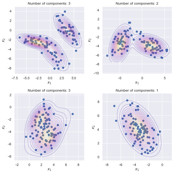
Figure 1: Samples and level curves for sample GMMs in the mode classification experiment, with $r=2$, $C=3$ and $n=100$.

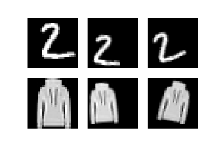
Figure 2: Sample transformations applied to MNIST (Top row) and Fashion MNIST (Bottom row) images. (Left column) raw $28\times 28$ pixel images. Images are padded to $34\times 34$ pixels and randomly roto-translated by degree drawn uniformly (for each image) on $[-15,15]$ (Middle column) and $[-30,30]$ (Right column.

Table 2: Mean accuracy and standard deviation on rotated MNIST and Fashion MNIST with maximum rotation $\theta_{\vee}=0,\pi/12,\pi/6$ respectively. Comparison between KRR estimators with standard Gaussian kernel (RBF), doubly Gaussian MMD kernel (MMD), a Gaussian ${\rm SW}_{2}$ kernel and a Gaussian ${\rm SW}_{1}$.

MNIST	RBF	MMD	${\rm SW}_{2}$	${\rm SW}_{1}$
Raw	$0.9~{}(0.01)$	$0.79~{}(0.03)$	$\mathbf{0.93~{}(0.01)}$	$0.91~{}(0.03)$
$\theta_{\vee}=\frac{\pi}{12}$	$0.51~{}(0.03)$	$0.40~{}(0.05)$	$\mathbf{0.85~{}(0.02)}$	$0.66~{}(0.02)$
$\theta_{\vee}=\frac{\pi}{6}$	$0.47~{}(0.03)$	$0.34~{}(0.04)$	$\mathbf{0.82~{}(0.01)}$	$0.61~{}(0.01)$

Fashion	RBF	MMD	${\rm SW}_{2}$	${\rm SW}_{1}$
Raw	$\mathbf{0.82~{}(0.01)}$	$0.75~{}(0.01)$	$0.81~{}(0.01)$	$0.77~{}(0.01)$
$\theta_{\vee}=\frac{\pi}{12}$	$0.66~{}(0.01)$	$0.48~{}(0.03)$	$\mathbf{0.74~{}(0.01)}$	$0.60~{}(0.02)$
$\theta_{\vee}=\frac{\pi}{6}$	$0.64~{}(0.01)$	$0.45~{}(0.01$)	$\mathbf{0.70~{}(0.01)}$	$0.58~{}(0.01$)

7 Conclusion

The main goal of this work was to address distribution regression from the perspective of Optimal Transport (OT), in contrast to the more common and well-established MMD-based strategies. For this purpose we proposed the first kernel ridge regression estimator for distribution regression, using Sliced Wasserstain distances to define a distance substitution kernel. We proved finite learning bounds for these estimators, extending previous work from Fang et al. (2020). We empirically evaluated our estimator on a number of real and simulations experiments, showing that tackling distribution regression with OT-based methods outperforms MMD-based approaches in several settings.

We identify two main directions for future research: firstly, we plan to better identify which regimes are more favorable for OT-based and MMD-based distribution regression. This is an open question in the literature and requires delving deeper in the analysis of the approximation properties of the distance substitution kernels induced by the two distances respectively. Secondly, our theoretical results, do not account for the fact that the Sliced Wasserstein distance needs to be approximated via Monte-Carlo methods. This analysis was beyond the scope of this work, which focuses on comparing OT and MMD based distribution regression. However, we plan to account for this further (third) sampling stage in future work.

Software and Data

Code is available at https://github.com/DimSum2k/DRSWK.

Supplementary Material

Below we give an overview of the structure of the supplementary material.

• Appendix A contains two derivations related to the distribution regression set up: the decomposition of the excess risk and the closed-form expression of the minimizer of the second-stage empirical risk.

• In Appendix B we present more examples of distance substitution kernels and the proof that $\sqrt{d_{{\rm SW}_{1}}}$ is Hilbertian.

• Appendix C contains the proof of Prop. 7 for ${\rm SW}_{1}$.

• In Appendix D we show how the Sliced Wasserstein distance can be computed and approximated in practice.

• Appendix E contains a discussion around the Hölder assumption and shows that it holds for $q:x\mapsto e^{-\gamma x^{2\beta}}$. Specifically, Sec. E.2 contains the proof of Thm. 8 and Sec. E.3 contains the proof of Cor. 9.

• Appendix F contains the details of the choice of hyperparameters for the experimental section.

• Appendix G contains additional experiments with the Hellinger and total variation distances.

Appendix A Distribution Kernel Ridge Regression

Proposition 11.

For all $f:X\rightarrow\mathbb{R}$ measurable,

$$\mathcal{E}(f):=\int_{X\times Y}(f(\mathbb{P})-y)^{2}d\rho(\mathbb{P},y)=\|f-f_{\rho}\|_{L^{2}_{\rho_{X}}}^{2}+\mathcal{E}(f_{\rho}).$$

The second term is independent of $f$ and the first term is minimised for $f=f_{\rho}$ a.e. which implies

$$f_{\rho}(\mathbb{P})=\operatorname*{argmin}_{f}\mathcal{E}(f)=\operatorname*{argmin}_{f}\|f-f_{\rho}\|_{L^{2}_{\rho_{X}}}.$$

Proof.

$$\int_{X\times Y}(f(\mathbb{P})-y)^{2}d\rho(\mathbb{P},y) =\int_{X\times Y}(f(\mathbb{P})-f_{\rho}(\mathbb{P})+f_{\rho}(\mathbb{P})-y)^{2}d\rho(\mathbb{P},y)$$

$$=\int_{X}(f(\mathbb{P})-f_{\rho}(\mathbb{P}))^{2}d\rho_{X}(\mathbb{P})+2\int_{X\times Y}(f(\mathbb{P})-f_{\rho}(\mathbb{P}))(f_{\rho}(\mathbb{P})-y)d\rho(\mathbb{P},y)+\mathcal{E}(f_{\rho})$$

$$=\|f-f_{\rho}\|_{L^{2}_{\rho_{X}}}^{2}+2\int_{X}(f(\mathbb{P})-f_{\rho}(\mathbb{P}))(f_{\rho}(\mathbb{P})-\underbrace{\int_{Y}yd\rho_{Y\mid X}(y\mid\mathbb{P})}_{=f_{\rho(\mathbb{P})}})d\rho_{X}(\mathbb{P})+\mathcal{E}(f_{\rho})$$

$$=\|f-f_{\rho}\|_{L^{2}_{\rho_{X}}}^{2}+\mathcal{E}(f_{\rho})$$

∎

The following proposition shows how to derive the explicit form of the minimizer of the second-stage empirical risk 4.

Proposition 12.

Let $K:X\times X\to\mathbb{R}$ be a p.d. kernel with RKHS denoted as $\mathcal{H}_{K}$, then

$$f_{\hat{\mathcal{D}},\lambda}=\operatorname*{argmin}_{f\in\mathcal{H}_{K}}\frac{1}{T}\sum_{t=1}^{T}\left(f\left(\hat{\mathbb{P}}_{t,n_{t}}\right)-y_{t}\right)^{2}+\lambda\|f\|_{\mathcal{H}_{K}}^{2}$$ (17)

takes the form

$$f_{\hat{\mathcal{D}},\lambda}(\mathbb{P})=(y_{1},\ldots,y_{T})(K_{T}+\lambda TI_{T})^{-1}k_{\mathbb{P}},\quad\forall\mathbb{P}\in X$$

where $[K_{T}]_{t,l}=K\left(\hat{\mathbb{P}}_{t,n_{t}},\hat{\mathbb{P}}_{l,n_{l}}\right)\in\mathbb{R}^{T\times T}$ and $k_{\mathbb{P}}=\left(K\left(\mathbb{P},\hat{\mathbb{P}}_{1,n_{1}}\right),\ldots,K\left(\mathbb{P},\hat{\mathbb{P}}_{T,n_{T}}\right)\right)^{\top}\in\mathbb{R}^{T}$.

Proof.

By the representer theorem Schölkopf et al. (2001) a minimizer of the empirical risk takes the form $f_{\alpha}(\cdot)=\sum_{t=1}^{T}\alpha_{t}K(\hat{\mathbb{P}}_{t,n_{t}},\cdot)$. The minimisation of the empirical risk is therefore equivalent to

$$\alpha^{*} =\operatorname*{argmin}_{\alpha\in\mathbb{R}^{T}}\|K_{T}\alpha-y\|_{\mathbb{R}^{T}}^{2}+\lambda T\alpha^{\top}K_{T}\alpha$$

$$=\operatorname*{argmin}_{\alpha\in\mathbb{R}^{T}}\alpha^{T}K_{T}\left(K_{T}+\lambda TI_{T}\right)\alpha-2y^{\top}K_{T}\alpha.$$

Taking the gradient with respect to $\alpha$, we obtain the first order condition $K_{T}\left[(K_{T}+\lambda TI_{T})\alpha-y\right]=0$. Hence any solution takes the form

$$\alpha^{\prime}=\underbrace{(K_{T}+\lambda TI_{T})^{-1}y}_{=:\alpha^{*}}+\epsilon,\text{ with }K_{T}\epsilon=0.$$

When $K_{T}$ is singular we have an infinity of solutions, however, they all lead to the same solution in $\mathcal{H}_{K}$. Indeed, if $\alpha^{\prime}=\alpha^{*}+\epsilon$ with $K_{T}\epsilon=0$, then:

$$\left\|f_{\alpha^{\prime}}-f_{\alpha^{*}}\right\|_{\mathcal{H}_{K}}^{2}=\left(\alpha^{\prime}-\alpha^{*}\right)^{\top}K_{T}\left(\alpha^{\prime}-\alpha^{*}\right)=0$$

therefore $f_{\alpha^{\prime}}=f_{\alpha^{*}}$. It shows that Kernel Ridge Regression has a unique solution $f^{*}\in\mathcal{H}_{K}$ defined by

$$f^{*}(\mathbb{P})=(y_{1},\ldots,y_{T})(K_{T}+\lambda TI_{T})^{-1}k_{\mathbb{P}},\quad\left(\mathbb{P}\in X\right)$$

which can potentially be expressed by several $\alpha$’s if $K_{T}$ is singular. ∎

Appendix B Distance substitution kernels

Proposition 13 (Proposition 1 (Haasdonk & Bahlmann, 2004)).

For a set $M$ and a pseudo-distance distance $d$ on $M$, the following statements are equivalent:

• $d$ is a Hilbertian pseudo-distance;

• $K_{lin}(x,y)=\langle x,y\rangle_{d}^{x_{0}}$, for all $x_{0}\in M$, $(x,y)\in M^{2}$ is p.d.;

• $K_{poly}(x,y)=(c+\langle x,y\rangle_{d}^{x_{0}})^{\ell}$ for all $c\geq 0$ and $\ell\in\mathbb{N}$, $(x,y)\in M^{2}$ is p.d.;

• $K(x,y)=\exp(-\gamma d^{2\beta}(x,y))$ for all $\gamma\geq 0,\beta\in[0,1]$, $(x,y)\in M^{2}$ is p.d.;

We can therefore embed Hilbertian pseudo-distances in polynomial-like, Laplace-like ($\beta=1/2$) and Gaussian-like ($\beta=1$) kernels. Furthermore Szabó et al. (2016) provides examples of Cauchy-like, t-student-like and inverse multiquadratic-like kernels.

We now prove that $\sqrt{d_{{\rm SW}_{1}}}$ is Hilbertian by showing that $d_{{\rm SW}_{1}}$ is conditionally negative definite (c.n.d). We first recall the definition of a c.n.d function and how it relates to Hilbertian pseudo-distances.

Definition 2.

Let $M$ be a set. A map $f:M\times M\rightarrow\mathbb{R}$ is called conditionally negative definite (c.n.d.) if and only if it is symmetric and satisfies:

$$\sum_{i,j=1}^{n}a_{i}a_{j}f(x_{i},x_{j})\leq 0$$

for any $n\in\mathbb{N}$, $(x_{1},\ldots,x_{n})\in M^{n}$ and $(a_{1},\ldots,a_{n})\in\mathbb{R}^{n}$ with $\sum_{i=1}^{n}a_{i}=0$.

Square of Hilbertian pseudo-distances are c.n.d.

Proposition 14.

Let $\Phi:M\to\mathcal{F}$ be a mapping to a Hilbert space $\mathcal{F}$ and $f(x,y)=\|\Phi(x)-\Phi(y)\|^{2}_{\mathcal{F}}$, then $f$ is c.n.d.

Proof.

$f$ is symmetric and for $n\in\mathbb{N}$, $(a_{1},\dots,a_{n})\in\mathbb{R}^{n}$, $(x_{1},\dots,x_{n})\in M^{n}$, we have:

$$\sum_{1\leq i,j\leq n}a_{i}a_{j}f(x_{i},x_{j}) =\sum_{1\leq i,j\leq n}a_{i}a_{j}\left(\|\Phi(x_{i})\|^{2}+\|\Phi(x_{j})\|^{2}-2\langle\Phi(x_{i}),\Phi(x_{j})\rangle\right)$$

$$=2\left(\sum_{i=1}^{n}a_{i}\|\Phi(x_{i})\|^{2}\right)\left(\sum_{j=1}^{n}a_{j}\right)-2\left\|\sum_{i=1}^{n}a_{i}\Phi(x_{i})\right\|^{2}$$

Under the constraint $\sum_{i=1}^{n}a_{i}=0$, the first term disappears and only a nonpositive term remains. Hence, $f:(x,y)\mapsto\|\Phi(x)-\Phi(y)\|^{2}$ is c.n.d. ∎

A corollary of Schoenberg’s theorem (see chapter 3 in (Berg et al., 1984)) shows that the converse holds.

Proposition 15.

Let $f$ be a c.n.d. function on $M$ such that $f(x,x)=0$ for any $x\in M$. Then, there exists a Hilbert space $\mathcal{F}$ and a mapping $\Phi:M\rightarrow\mathcal{F}$ such that for any $(x,y)\in M^{2}$,

$$f(x,y)=||\Phi(x)-\Phi(y)||^{2}_{\mathcal{F}}.$$

As a consequence showing that $\sqrt{d_{{\rm SW}_{1}}}$ is Hilbertian is equivalent to showing that $d_{{\rm SW}_{1}}$ is c.n.d. We start with the following lemma.

Lemma 16.

Let $M$ be a set, $(\Omega,\mathcal{A},\mu)$ a measurable space and $\phi:M\times\Omega\to\mathbb{R}$ be such that $\phi(x,\cdot)\in L_{1}(\mu)$ for all $x\in M$. Then, $f:M\times M\to\mathbb{R},(x,y)\mapsto\int_{\Omega}|\phi(x,\omega)-\phi(y,\omega)|d\mu(\omega)$ is c.n.d.

Proof.

First, notice that for all $(u,v)\in[a,+\infty)$, $\displaystyle\min(u,v)=\int_{a}^{+\infty}1_{t\leq u}1_{t\leq v}dt+a$. Secondly, for all $u,v\in\mathbb{R}$, $|u-v|=u+v-2\min(u,v)$. For all $n\in\mathbb{N}^{*}$, $(x_{1},\ldots,x_{n})\in M^{n}$ and $\omega\in\Omega$ define $a_{n}^{\omega}:=a(\omega;x_{1},\ldots,x_{n}):=\min_{i=1,\ldots,n}\phi(x_{i},\omega)$. For all $(a_{1},\ldots,a_{n})\in\mathbb{R}^{n}$ such that $\sum_{i=1}^{n}a_{i}=0$,

$$\sum_{i,j=1}^{n}a_{i}a_{j}f(x_{i},x_{j}) =\int_{\Omega}\sum_{i,j=1}^{n}a_{i}a_{j}\left\{\phi(x_{i},\omega)+\phi(x_{j},\omega)-2\min(\phi(x_{i},\omega),\phi(x_{j},\omega))\right\}d\mu(\omega)$$

$$=-2\int_{\Omega}\sum_{i,j=1}^{n}a_{i}a_{j}\min(\phi(x_{i},\omega),\phi(x_{j},\omega))d\mu(\omega)\qquad\text{ since }\sum_{i=1}^{n}a_{i}=0$$

$$=-2\int_{\Omega}\sum_{i,j=1}^{n}a_{i}a_{j}\left(\int_{a_{n}^{\omega}}^{+\infty}1_{t\leq\phi(x_{i},\omega)}1_{t\leq\phi(x_{j},\omega)}dt+a_{n}^{\omega}\right)d\mu(\omega)$$

$$=-2\int_{\Omega}\int_{a_{n}^{\omega}}^{+\infty}\left(\sum_{i=1}^{n}a_{i}1_{t\leq\phi(x_{i},\omega)}\right)^{2}dt+\left(\sum_{i=1}^{n}a_{i}\right)^{2}a_{n}^{\omega}d\mu(\omega)$$

$$=-2\int_{\Omega}\int_{a_{n}^{\omega}}^{+\infty}\left(\sum_{i=1}^{n}a_{i}1_{t\leq\phi(x_{i},\omega)}\right)^{2}dtd\mu(\omega)\qquad\text{ since }\sum_{i=1}^{n}a_{i}=0$$

$$\leq 0$$

which proves that $f$ is c.n.d. ∎

Applying the result to $d_{W_{1}}(\mathbb{P},\mathbb{Q})=\int_{0}^{1}|F_{\mathbb{P}}^{[-1]}(x)-F_{\mathbb{Q}}^{[-1]}(x)|dx$ shows that $d_{W_{1}}$ is c.n.d. We conclude that $d_{{\rm SW}_{1}}$ is c.n.d by linearity of the integral.

Proposition 17.

$d_{{\rm SW}_{1}}(\mathbb{P},\mathbb{Q})=\int_{\mathbb{S}^{r-1}}d_{W_{1}}\left(\theta^{*}_{\#}\mathbb{P},\theta^{*}_{\#}\mathbb{Q}\right)d\theta$ is c.n.d.

Proof.

For all $n\in\mathbb{N}$, $(a_{1},\dots,a_{n})\in\mathbb{R}^{n}$ such that $\sum_{i=1}^{n}a_{i}=0$ and $(\mathbb{P}_{1},\dots,\mathbb{P}_{n})\in X^{n}$,

$$\sum_{1\leq i,j\leq n}a_{i}a_{j}d_{{\rm SW}_{1}}(\mathbb{P}_{i},\mathbb{P}_{j})=\int_{\mathbb{S}^{r-1}}\underbrace{\sum_{1\leq i,j\leq n}a_{i}a_{j}d_{W_{1}}\left(\theta^{*}_{\#}\mathbb{P}_{i},\theta^{*}_{\#}\mathbb{P}_{j}\right)}_{\leq 0}d\theta\leq 0.$$

∎

Hence by Prop. 15, $\sqrt{d_{{\rm SW}_{1}}}$ is Hilbertian. It is important to observe that the proof that $\sqrt{d_{{\rm SW}_{1}}}$ is Hilbertian does not lead to an explicit feature map and feature space while for $d_{{\rm SW}_{2}}$ we have an explicit construction.

Appendix C Universality with ${\rm SW}_{1}$

Proposition 18.

$K_{1}:X\times X\to\mathbb{R},(\mathbb{P},\mathbb{Q})\mapsto e^{-\gamma{\rm SW}_{1}(\mathbb{P},\mathbb{Q})}$ is universal for $(X,d_{LP})$ where $d_{LP}$ is the Lévy–Prokhorov distance.

Since we do not know explicitely the feature map nor the feature space for $\sqrt{d_{{\rm SW}_{1}}}$ we need to take a little detour for the separability requirement.

Proof.

Since $\sqrt{d_{{\rm SW}_{1}}}$ is Hilbertian, there is a feature map $\Phi:\mathcal{M}_{+}^{1}(\Omega_{r})\to\mathcal{F}$ where $\mathcal{F}$ is a Hilbert space such that $\sqrt{d_{{\rm SW}_{1}}}(\mathbb{P},\mathbb{Q})=\|\Phi(\mathbb{P})-\Phi(\mathbb{Q})\|_{\mathcal{F}}$. Since $d_{{\rm SW}_{1}}$ satisfies the identity of indiscernibles, $\sqrt{d_{{\rm SW}_{1}}}$ too, which implies that $\Phi$ is injective and hence $\sqrt{d_{{\rm SW}_{1}}}$ is a distance. (Nadjahi et al., 2019) showed that $d_{{\rm SW}_{1}}$ metrizes the weak convergence and by continuity of the square root $\sqrt{d_{{\rm SW}_{1}}}$ too. Therefore, we can reason as for $K_{2}$ except that we need to show that $\mathcal{F}$ is separable. By Proposition 2.2 (Smola & Schölkopf, 1998), $\mathcal{F}$ can be chosen as the RKHS induced by the kernel

$$\tilde{k}(\mathbb{P},\mathbb{Q})=d_{{\rm SW}_{1}}(\mathbb{P}_{0},\mathbb{P})+d_{{\rm SW}_{1}}(\mathbb{P}_{0},\mathbb{Q})-d_{{\rm SW}_{1}}(\mathbb{P},\mathbb{Q})=2\langle\Phi(\mathbb{P})-\Phi(\mathbb{P}_{0}),\Phi(\mathbb{Q})-\Phi(\mathbb{P}_{0})\rangle_{\mathcal{F}}.$$

for $\mathbb{P}_{0}\in\mathcal{M}_{+}^{1}(\Omega_{r})$. By Lemma 4.33 in (Steinwart & Christmann, 2008), if the input space is separable and $\tilde{k}$ is continuous then the RKHS is separable. Here the input space is $\mathcal{M}_{+}^{1}(\Omega_{r})$ which is weakly compact (since we have assumed $\Omega_{r}$ compact) hence weakly separable. Furthermore $\Phi$ continuous w.r.t $\sqrt{d_{{\rm SW}_{1}}}$ implies $\tilde{k}$ continuous (Lemma 4.29 in (Steinwart & Christmann, 2008)). ∎

Appendix D Practical implementation of the Sliced Wasserstein kernel

Computing SW kernel values requires to evaluate the SW distance. In this section we detail how. The following lemma explain how the generalised inverse of the cumulative distribution function of an empirical measure can be evaluated.

Lemma 19.

We consider the distribution $\hat{\alpha}=\sum_{k=1}^{+\infty}p_{k}\delta_{x_{k}}$ where $(x_{k})_{k\geq 1}\in\mathbb{R}^{\mathbb{N}}$ and $(p_{k})_{k\geq 1}\in\mathbb{R}^{\mathbb{N}}_{+}$ such that $\sum_{k\geq 1}p_{k}=1$. We refer to the sorted sequence as $(x_{(k)})_{k\geq 1}\in\mathbb{R}^{\mathbb{N}}$ with reordered weights $(p_{(k)})_{k\geq 1}$ and define $\displaystyle s_{k}=\sum_{i=1}^{k}p_{(i)}$, $s_{0}=0$. Then, we have

$$F_{\hat{\alpha}}(x)=\mathbb{P}_{\hat{\alpha}}(X\leq x)=\sum_{k=1}^{+\infty}p_{k}1_{x_{k}\leq x}=s_{\max(k\mid x_{(k)}\leq x)}\qquad\left(x\in\mathbb{R}\right),$$

$$F_{\hat{\alpha}}^{[-1]}(t)=\inf\left\{x\in\mathbb{R}:\sum_{k=1}^{+\infty}p_{k}1_{x_{k}\leq x}\geq t\right\}=\{x_{(k)}\mid s_{k-1}<t\leq s_{k},k\geq 1\},\qquad F_{\hat{\alpha}}^{[-1]}(0)=-\infty.$$

In particular, for a uniform empirical distribution on a set of $n$ points $\displaystyle\hat{\alpha}=\frac{1}{n}\sum_{i=1}^{n}\delta_{x_{i}}$, we get

$$F_{\hat{\alpha}}(x) =\frac{\max(k\mid x_{(k)}\leq x)}{n}\qquad\left(x\in\mathbb{R}\right),$$ (18)

$$F_{\hat{\alpha}}^{[-1]}(t) =x_{(k)}\quad\text{ if }\frac{k-1}{n}<t\leq\frac{k}{n}\quad 1\leq k\leq n\quad-\infty\text{ if }t=0\quad\left(t\in[0,1]\right).$$

$F_{\hat{\alpha}}^{[-1]}(t)$ is a piece-wise constant function on the uniform grid with step $\displaystyle\left(\frac{k-1}{n},\frac{k}{n}\right],1\leq k\leq n$.

We can use 18 to compute the W distance and approximate the SW distance between empirical distributions.

Balanced setting.

For two empirical distributions with the same number of points: $\displaystyle\hat{\alpha}=\frac{1}{n}\sum_{i=1}^{n}\delta_{x_{i}}$, $\displaystyle\hat{\beta}=\frac{1}{n}\sum_{i=1}^{n}\delta_{y_{i}}$, $x_{i},y_{i}\in\mathbb{R}$ exploiting 18, we get

$$d_{W_{p}}(\hat{\alpha},\hat{\beta})^{p} =\int_{0}^{1}\left|F_{\hat{\alpha}}^{[-1]}(t)-F_{\hat{\beta}}^{[-1]}(t)\right|^{p}dt$$ (19)

$$=\sum_{k=1}^{n}\int_{\frac{k-1}{n}}^{k/n}\left|F_{\hat{\alpha}}^{[-1]}(t)-F_{\hat{\beta}}^{[-1]}(t)\right|^{p}dt$$

$$=\sum_{k=1}^{n}\int_{\frac{k-1}{n}}^{k/n}\left|x_{(k)}-y_{(k)}\right|^{p}dt$$

$$=\frac{1}{n}\sum_{k=1}^{n}\left|x_{(k)}-y_{(k)}\right|^{p}$$

Now we consider $\displaystyle\hat{\alpha}=\frac{1}{n}\sum_{i=1}^{n}\delta_{x_{i}}$, $\displaystyle\hat{\beta}=\frac{1}{n}\sum_{i=1}^{n}\delta_{y_{i}}$, with points in $\mathbb{R}^{r}$ instead of $\mathbb{R}$. We recall that for $\theta\in S^{r-1}$, we denote by $\theta^{*}$ the map $\theta^{*}:\mathbb{R}^{r}\to\mathbb{R},x\mapsto\langle x,\theta\rangle$ and by $\theta^{*}_{\#}$ the associated push-forward operator. We have $\theta^{*}_{\#}\alpha=\frac{1}{n}\sum_{i=1}^{n}\delta_{\langle x_{i},\theta\rangle}$. We denote by $(x_{(i)}^{\theta})_{i=1}^{n}$ the sorted sequence after projection, i.e. $x_{i}^{\theta}:=\langle x_{i},\theta\rangle$ for all $i=1,\ldots,n$ and

$$x_{(1)}^{\theta}\leq\ldots\leq x_{(n)}^{\theta}$$ (20)

By 19 the Sliced Wasserstein distance is given by

$$d_{{\rm SW}_{p}}(\hat{\alpha},\hat{\beta})^{p}=\frac{1}{n}\sum_{k=1}^{n}\int_{S^{r-1}}\left|x_{(k)}^{\theta}-y_{(k)}^{\theta}\right|^{p}d\theta$$ (21)

which can be approximated as

$$d_{{\rm SW}_{p}}(\hat{\alpha},\hat{\beta})^{p}\approx\frac{1}{nM}\sum_{m=1}^{M}\sum_{k=1}^{n}\left|x_{(k)}^{\theta_{m}}-y_{(k)}^{\theta_{m}}\right|^{p}$$ (22)

where $\theta_{m}\sim^{i.i.d}\mathcal{U}(S^{d-1})$.

Unalanced setting.

For two empirical distributions: $\displaystyle\hat{\alpha}=\frac{1}{n}\sum_{i=1}^{n}\delta_{x_{i}}$, $\displaystyle\hat{\beta}=\frac{1}{m}\sum_{i=1}^{m}\delta_{y_{i}}$, $x_{i},y_{i}\in\mathbb{R}$, as the functions $F_{\hat{\alpha}}^{[-1]}$ and $F_{\hat{\beta}}^{[-1]}$ are piece-wise constant functions on the uniform grid with respectively $n$ and $m$ points, $t\mapsto\left|F_{\hat{\alpha}}^{[-1]}(t)-F_{\hat{\beta}}^{[-1]}(t)\right|$ is piece-wise constant on the intervals defined by the intersection of the two uniform grids and the value it takes on each interval is given by the ordered sequences. The computation of $d_{W_{p}}(\hat{\alpha},\hat{\beta})^{p}$ and the approximation of $d_{{\rm SW}_{p}}(\hat{\alpha},\hat{\beta})^{p}$ when we go to $\mathbb{R}^{r}$ is therefore performed in a fashion similar to the balanced setting. The only additional step is to deal with the intersection of the grids.

Appendix E Main proofs of Sec. 5

E.1 Discussion around the Hölder assumption

Assumption 16 might make the reader think that its validity depends on the chosen Hilbertian metric $d$ while it does not. Indeed, as noticed in Szabó et al. (2015) we can write

$$\|K_{\mathbb{P}}-K_{\mathbb{Q}}\|_{\mathcal{H}_{K}}^{2} =K(\mathbb{P},\mathbb{P})+K(\mathbb{Q},\mathbb{Q})-2K(\mathbb{P},\mathbb{Q})$$

$$=2\left(q(0)-q(d(\mathbb{P},\mathbb{Q}))\right).$$

Therefore, the Hölder condition on $K$ can be replaced by a regularity condition on $q$ only. There are constants $L>0$ and $h\in(0,1]$ such that

$$\frac{q(0)-q(x)}{x^{2h}}\leq L,\quad\forall x\in\mathbb{R}_{+}^{*}$$ (23)

which is independent of the underlying distance $d$. For example, it holds with $h=\beta$ for $q:x\mapsto e^{-\gamma x^{2\beta}}$ as shown below in Prop. 20. Inequality 16 is important as the derivations for the excess risk bound involve multiple times the difference $\|K_{\mathbb{P}}-K_{\hat{\mathbb{P}}_{n}}\|_{\mathcal{H}_{K}}$ which can be controlled by $d(\mathbb{P},\hat{\mathbb{P}}_{n})$ thanks to the regularity assumption.

Proposition 20.

For $\gamma>0$ and $\beta\in[0,1]$, $q:\mathbb{R}_{+}\to\mathbb{R},x\mapsto e^{-\gamma x^{2\beta}}$ satisfies

$$\frac{q(0)-q(x)}{x^{2h}}\leq L,\quad\forall x\in\mathbb{R}_{+}^{*}$$

for $h=\beta$ and some $L>0$.

Proof.

$x\to\frac{q(0)-q(x)}{x^{2h}}$ is continuous and goes to $0$ as $x$ goes to $+\infty$. Therefore it remains to show that the limit exists when $x\to 0^{+}$. By L’Hôpital’s rule,

$$\lim_{x\rightarrow 0^{+}}\frac{q(0)-q(x)}{x^{2h}}=\lim_{x\rightarrow 0^{+}}\frac{1-e^{-\gamma x^{2\beta}}}{x^{2h}}=\lim_{x\rightarrow 0^{+}}\frac{\gamma\beta x^{2\beta-1}e^{-\gamma x^{2\beta}}}{hx^{2h-1}}$$

The largest $h$ for which the limit exists is $h=\beta$. ∎

E.2 Proof of the main theorem

Before proving the main theorem we introduce the approximations of the integral operator.

Integral operator approximations.

Given the first and second stage sampling inputs we introduce the operators

$$\Phi_{\mathcal{D}}\colon\mathbb{R}^{T} \rightarrow\mathcal{H}_{K}\qquad \Phi_{\hat{\mathcal{D}}}\colon\mathbb{R}^{T} \rightarrow\mathcal{H}_{K}$$

$$\alpha \mapsto\sum_{t=1}^{T}\alpha_{t}K_{\mathbb{P}_{t}}\qquad \alpha \mapsto\sum_{t=1}^{T}\alpha_{t}K_{\hat{\mathbb{P}}_{t,n}}$$

their adjoint operators are the first and second stage sampling operators

$$\Phi_{\mathcal{D}}^{*}\colon\mathcal{H}_{K} \rightarrow\mathbb{R}^{T}\qquad \Phi_{\hat{\mathcal{D}}}^{*}\colon\mathcal{H}_{K} \rightarrow\mathbb{R}^{T}$$

$$f \mapsto f(\mathbb{P}_{t})_{t=1}^{T}\qquad f \mapsto f(\hat{\mathbb{P}}_{t,n})_{t=1}^{T}$$

The integral operator is approximated at first and second stage respectively by $L_{K,\mathcal{D}}:=\frac{1}{T}\Phi_{\mathcal{D}}\circ\Phi_{\mathcal{D}}^{*}$ and
$L_{K,\hat{\mathcal{D}}}:=\frac{1}{T}\Phi_{\hat{\mathcal{D}}}\circ\Phi_{\hat{\mathcal{D}}}^{*}$.

$$L_{K,\mathcal{D}}\colon\mathcal{H}_{K} \rightarrow\mathcal{H}_{K}\qquad \L_{K,\hat{\mathcal{D}}}\colon\mathcal{H}_{K} \rightarrow\mathcal{H}_{K}$$

$$f \mapsto\frac{1}{T}\sum_{t=1}^{T}f(\mathbb{P}_{t})K_{\mathbb{P}_{t}}\qquad f \mapsto\frac{1}{T}\sum_{t=1}^{T}f(\hat{\mathbb{P}}_{t,n})K_{\hat{\mathbb{P}}_{t,n}}$$

The introduction of the integral operator and its approximations from finite samples is convenient as we can express the solution of the regularized empirical risk minimization problems as follows,

$$f_{\mathcal{D},\lambda}=(L_{K,\mathcal{D}}+\lambda I)^{-1}\frac{\Phi_{\mathcal{D}}}{T}y\qquad f_{\hat{\mathcal{D}},\lambda}=(L_{K,\hat{\mathcal{D}}}+\lambda I)^{-1}\frac{\Phi_{\hat{\mathcal{D}}}}{T}y$$ (24)

Plan of the proof.

Our goal is to control $\mathcal{E}(f_{\hat{\mathcal{D}},\lambda})-\mathcal{E}(f_{\rho})$ the expected excess risk. But since $\mathcal{E}$ can be decomposed as

$$\mathcal{E}(f)=\|f-f_{\rho}\|_{L^{2}_{\rho_{X}}}^{2}+\mathcal{E}(f_{\rho}),$$ (25)

we will consider the decomposition

$$\left(\mathcal{E}(f_{\hat{\mathcal{D}},\lambda})-\mathcal{E}(f_{\rho})\right)^{1/2} =\|f_{\hat{\mathcal{D}},\lambda}-f_{\rho}\|_{L_{2}}$$ (26)

$$\leq\underbrace{\|f_{\hat{\mathcal{D}},\lambda}-f_{\mathcal{D},\lambda}\|_{L^{2}}}_{=:B}+\underbrace{\|f_{\mathcal{D},\lambda}-f_{\rho}\|_{L_{2}}}_{=:A}.$$

Both terms can be written in terms of the integral operator and its approximations as defined previously,

$$A =\|f_{\mathcal{D},\lambda}-f_{\rho}\|_{L^{2}}=\left\|L_{K}^{1/2}\left((L_{K,\mathcal{D}}+\lambda I)^{-1}\frac{\Phi_{\mathcal{D}}}{T}y-(L_{K,\mathcal{D}}+\lambda I)^{-1}(L_{K,\mathcal{D}}+\lambda I)f_{\rho}\right)\right\|_{\mathcal{H}_{K}}$$ (27)

$$\leq\left\|L_{K}^{1/2}(L_{K,\mathcal{D}}+\lambda I)^{-1}\left(\frac{\Phi_{\mathcal{D}}}{T}y-L_{K,\mathcal{D}}f_{\rho}\right)\right\|_{\mathcal{H}_{K}}+\lambda\left\|L_{K}^{1/2}(L_{K,\mathcal{D}}+\lambda I)^{-1}L_{K}^{1/2}g_{\rho}\right\|_{\mathcal{H}_{K}}.$$

Where we used the isometry $L_{K}^{1/2}$ and that since $f_{\rho}\in\mathcal{H}_{K}$, $f_{\rho}=L_{K}^{1/2}(g_{\rho})$ for some $g_{\rho}\in L^{2}_{\rho_{X}}$. Those quantities do not depend on the sampling rate of the chosen distance for the kernel. Bounding the expected value of $A$ boils down to control for $\mathbb{E}\left[\left\|(L_{K}+\lambda I)(L_{K,\mathcal{D}}+\lambda I)^{-1}\right\|\right]$ and $\mathbb{E}\left[\left\|(L_{K}+\lambda I)^{-1}\left(\frac{\Phi_{\mathcal{D}}}{T}y-L_{K,\mathcal{D}}f_{\rho}\right)\right\|\right]$, Proposition 5 Fang et al. (2020). This can be obtained through concentration inequalities. Term A is the excess risk for standard Kernel Ridge Regression (1-stage sampling) and we can directly plug known results, for example Lemma 4 Fang et al. (2020):

$$E\left[\left\|f_{\mathcal{D},\lambda}-f_{\rho}\right\|_{L^{2}}\right]\leq C\left\{\left(\frac{\mathcal{B}_{T,\lambda}}{\sqrt{\lambda}}+1\right)^{2}\frac{A}{\kappa}\mathcal{B}_{T,\lambda}+\left\|g_{\rho}\right\|_{L_{2}}\left(\mathcal{B}_{T,\lambda}+\sqrt{\lambda}\right)\right\},$$ (28)

where $C$ is a constant that does not depend on any parameter, $\mathcal{B}_{T,\lambda}=\frac{2\kappa}{\sqrt{T}}\left(\frac{\kappa}{\sqrt{T\lambda}}+\sqrt{\mathcal{N}(\lambda)}\right)$, $\mathcal{N}(\lambda)$ is the effective dimension, $\mathcal{N}(\lambda)=\operatorname{Tr}\left(L_{K}\left(L_{K}+\lambda I\right)^{-1}\right)$ $\forall\lambda>0$ and $A$ is such that $|y|\leq A$, $\rho$ a.s.

Term B is the error induced by the fact that we only access the covariates $(\mathbb{P}_{t})_{t=1}^{T}$ through empirical approximations $(\hat{\mathbb{P}}_{t,n})_{t=1}^{T}$, this term is specific to distribution regression. We follow a decomposition of $B$ similar to the one used in (Fang et al., 2020), but while they focused on MMD-based kernels we adapt the decomposition to incorporate the sample rate of any distance substitution kernels.

$$B =\|f_{\hat{\mathcal{D}},\lambda}-f_{\mathcal{D},\lambda}\|_{L^{2}_{\rho_{X}}}=\left\|(L_{K,\hat{\mathcal{D}}}+\lambda I)^{-1}\frac{\Phi_{\hat{\mathcal{D}}}}{T}y-(L_{K,\mathcal{D}}+\lambda I)^{-1}\frac{\Phi_{\mathcal{D}}}{T}y\right\|_{L^{2}_{\rho_{X}}}$$ (29)

$$=\left\|(L_{K,\hat{\mathcal{D}}}+\lambda I)^{-1}\left(\frac{\Phi_{\hat{\mathcal{D}}}}{T}y-\frac{\Phi_{\mathcal{D}}}{T}y\right)+\left((L_{K,\hat{\mathcal{D}}}+\lambda I)^{-1}-(L_{K,\mathcal{D}}+\lambda I)^{-1}\right)\frac{\Phi_{\mathcal{D}}}{T}y\right\|_{L^{2}_{\rho_{X}}}$$

$$=\left\|(L_{K,\hat{\mathcal{D}}}+\lambda I)^{-1}\left(\frac{\Phi_{\hat{\mathcal{D}}}}{T}y-\frac{\Phi_{\mathcal{D}}}{T}y\right)+(L_{K,\hat{\mathcal{D}}}+\lambda I)^{-1}\left(L_{K,\mathcal{D}}-L_{K,\hat{\mathcal{D}}}\right)f_{\mathcal{D},\lambda}\right\|_{L^{2}}$$

$$\leq\underbrace{\left\|L_{K}^{1/2}(L_{K,\hat{\mathcal{D}}}+\lambda I)^{-1}\left(\frac{\Phi_{\hat{\mathcal{D}}}}{T}y-\frac{\Phi_{\mathcal{D}}}{T}y\right)\right\|_{\mathcal{H}_{K}}}_{=:C}+\underbrace{\left\|L_{K}^{1/2}(L_{K,\hat{\mathcal{D}}}+\lambda I)^{-1}\left(L_{K,\mathcal{D}}-L_{K,\hat{\mathcal{D}}}\right)f_{\mathcal{D},\lambda}\right\|_{\mathcal{H}_{K}}}_{:=D}.$$

Where we used that for two invertible operators $A^{-1}-B^{-1}=A^{-1}(B-A)B^{-1}$, 24 and the isometry $L_{K}^{1/2}$. We aim at bounding $\mathbb{E}\|f_{\hat{\mathcal{D}},\lambda}-f_{\mathcal{D},\lambda}\|_{L^{2}}$ in expectation, and we will see that it involves the sample complexity $d(\mathbb{P},\hat{\mathbb{P}}_{n})$. Let us start with term $C$, by the Cauchy-Schwarz inequality,

$$\mathbb{E}[C] =\mathbb{E}\left[\left\|L_{K}^{1/2}(L_{K,\hat{\mathcal{D}}}+\lambda I)^{-1}\left(\frac{\Phi_{\hat{\mathcal{D}}}}{T}y-\frac{\Phi_{\mathcal{D}}}{T}y\right)\right\|_{\mathcal{H}_{K}}\right]$$ (30)

$$\leq\mathbb{E}\left[\left\|L_{K}^{1/2}(L_{K,\hat{\mathcal{D}}}+\lambda I)^{-1}\right\|_{op}\left\|\left(\frac{\Phi_{\hat{\mathcal{D}}}}{T}y-\frac{\Phi_{\mathcal{D}}}{T}y\right)\right\|_{\mathcal{H}_{K}}\right]$$

$$\leq\left(\mathbb{E}\left[\left\|L_{K}^{1/2}(L_{K,\hat{\mathcal{D}}}+\lambda I)^{-1}\right\|_{op}\right]^{2}\right)^{1/2}\left(\mathbb{E}\left[\left\|\frac{\Phi_{\hat{\mathcal{D}}}}{T}y-\frac{\Phi_{\mathcal{D}}}{T}y\right\|_{\mathcal{H}_{K}}\right]^{2}\right)^{1/2},$$

where $\|\cdot\|_{op}$ denotes the operator norm. For the second term we have,

$$\left(\mathbb{E}\left[\left\|\frac{\Phi_{\hat{\mathcal{D}}}}{T}y-\frac{\Phi_{\mathcal{D}}}{T}y\right\|_{\mathcal{H}_{K}}^{2}\right]\right)^{1/2} =\left(\mathbb{E}\left[\left\|\frac{1}{T}\sum_{t=1}^{T}y_{t}\left(K(\mathbb{P}_{t},\cdot)-K(\hat{\mathbb{P}}_{t,n},\cdot)\right)\right\|_{\mathcal{H}_{K}}\right]^{2}\right)^{1/2}$$ (31)

$$\leq\frac{A}{\sqrt{T}}\left(\sum_{t=1}^{T}\mathbb{E}\left\|K(\mathbb{P}_{t},\cdot)-K(\hat{\mathbb{P}}_{t,n})\right\|_{\mathcal{H}_{K}}^{2}\right)^{1/2}$$

$$\leq\frac{AL}{\sqrt{T}}\left(\sum_{t=1}^{T}\mathbb{E}\left[d(\mathbb{P}_{t},\hat{\mathbb{P}}_{t,n})^{2h}\right]\right)^{1/2}$$

$$\leq\frac{AL}{\sqrt{T}}\left(\sum_{t=1}^{T}\mathbb{E}\left[d(\mathbb{P}_{t},\hat{\mathbb{P}}_{t,n})^{2}\right]^{h}\right)^{1/2}$$

$$\leq AL\alpha(n)^{h/2}.$$

where we used the Jensen inequality ($h<1$), $|y|\leq A$, 16 and the control over the sample complexity of $d$. For the first term, Lemma 8 in Fang et al. (2020) shows

$$\left\|L_{K}^{1/2}(L_{K,\hat{\mathcal{D}}}+\lambda I)^{-1}\right\|^{2}_{op}\leq\frac{3\Sigma_{\mathcal{D}}^{2}}{\lambda^{2}}+\frac{3}{\lambda^{3}}\|L_{K,\mathcal{D}}-L_{K,\hat{\mathcal{D}}}\|^{2}_{op}+\frac{3}{\lambda},$$ (32)

where $\Sigma_{\mathcal{D}}=\left\|\left(L_{K}+\lambda I\right)^{-\frac{1}{2}}\left(L_{K}-L_{K,\mathcal{D}}\right)\right\|_{op}$. We now show that the middle term can be controlled with $\alpha(n)$. For all $f\in\mathcal{H}_{K}$,

$$\|(L_{K,\mathcal{D}}-L_{K,\hat{\mathcal{D}}})(f)\|^{2}_{\mathcal{H}_{K}} =\left\|\frac{1}{T}\sum_{t=1}^{T}K(\mathbb{P}_{t},\cdot)f(\mathbb{P}_{t})-K(\hat{\mathbb{P}}_{t,n},\cdot)f(\hat{\mathbb{P}}_{t,n})\right\|_{\mathcal{H}_{K}}^{2}$$ (33)

$$\leq\frac{1}{T}\sum_{t=1}^{T}\left\|K(\mathbb{P}_{t},\cdot)f(\mathbb{P}_{t})-K(\hat{\mathbb{P}}_{t,n})f(\hat{\mathbb{P}}_{t,n})\right\|_{\mathcal{H}_{K}}^{2}$$

$$\leq\frac{2}{T}\sum_{t=1}^{T}(f(\mathbb{P}_{t})-f(\hat{\mathbb{P}}_{t,n}))^{2}\left\|K(\mathbb{P}_{t},.)\right\|_{\mathcal{H}_{K}}^{2}+f(\hat{\mathbb{P}}_{t,n})^{2}\left\|K(\mathbb{P}_{t},.)-K(\hat{\mathbb{P}}_{t,n})\right\|_{\mathcal{H}_{K}}^{2}$$

$$\leq\frac{2\kappa^{2}}{T}\sum_{t=1}^{T}(f(\mathbb{P}_{t})-f(\hat{\mathbb{P}}_{t,n}))^{2}+\|f\|_{\mathcal{H}_{K}}^{2}\left\|K(\mathbb{P}_{t},.)-K(\hat{\mathbb{P}}_{t,n})\right\|_{\mathcal{H}_{K}}^{2}$$

$$\leq\frac{4\kappa^{2}L^{2}\|f\|_{\mathcal{H}_{K}}^{2}}{T}\sum_{t=1}^{T}d(\mathbb{P}_{t},\hat{\mathbb{P}}_{t,n})^{2h},$$

where we used that $K(\mathbb{P},\mathbb{P})$ is bounded by $\kappa^{2}$ for all $\mathbb{P}\in X$ and

$$f(\hat{\mathbb{P}}_{t,n})^{2} \leq\|f\|_{\mathcal{H}_{K}}^{2}\left\|K(\hat{\mathbb{P}}_{t,n},.)\right\|_{\mathcal{H}_{K}}^{2}\leq\|f\|_{\mathcal{H}_{K}}^{2}\kappa^{2},$$ (34)

$$\left(f(\mathbb{P}_{t})-f(\hat{\mathbb{P}}_{t,n})\right)^{2} \leq\|f\|_{\mathcal{H}_{K}}^{2}\left\|K(\mathbb{P}_{t},.)-K(\hat{\mathbb{P}}_{t,n},.)\right\|_{\mathcal{H}_{K}}^{2}\leq L^{2}\|f\|_{\mathcal{H}_{K}}^{2}d(\mathbb{P}_{t},\hat{\mathbb{P}}_{t,n})^{2h},$$

by the Hölder assumption. Hence,

$$\|L_{K,\mathcal{D}}-L_{K,\hat{\mathcal{D}}}\|^{2}_{op}\leq\frac{4\kappa^{2}L^{2}}{T}\sum_{t=1}^{T}d(\mathbb{P}_{t},\hat{\mathbb{P}}_{t,n})^{2h},$$ (35)

which implies

$$\mathbb{E}\left[\|L_{K,\mathcal{D}}-L_{K,\hat{\mathcal{D}}}\|^{2}_{op}\right]\leq\frac{4\kappa^{2}L^{2}}{T}\sum_{t=1}^{T}\mathbb{E}[d(\mathbb{P}_{t},\hat{\mathbb{P}}_{t,n})^{2h}]\leq 4\kappa^{2}L^{2}\alpha(n)^{h},$$ (36)

and finally

$$\mathbb{E}\left\|L_{K}^{1/2}(L_{K,\hat{\mathcal{D}}}+\lambda I)^{-1}\right\|^{2}_{op}\leq\frac{3\mathbb{E}\left[\Sigma_{\mathcal{D}}^{2}\right]}{\lambda^{2}}+\frac{12}{\lambda^{3}}L^{2}\kappa^{2}\alpha(n)^{h}+\frac{3}{\lambda}.$$ (37)

Putting the bounds together, we have

$$\mathbb{E}[C] \leq AL\alpha(n)^{h/2}\sqrt{\frac{3\mathbb{E}[\Sigma_{\mathcal{D}}^{2}]}{\lambda^{2}}+\frac{12}{\lambda^{3}}L^{2}\kappa^{2}\alpha(n)^{h}+\frac{3}{\lambda}}$$ (38)

$$\leq\sqrt{3}AL\alpha(n)^{h/2}\left(\frac{\mathbb{E}[\Sigma_{\mathcal{D}}^{2}]^{1/2}}{\lambda}+\frac{2}{\lambda^{3/2}}L\kappa\alpha(n)^{h/2}+\frac{1}{\sqrt{\lambda}}\right)$$

$$\leq\frac{\sqrt{3}AL\alpha(n)^{h/2}}{\sqrt{\lambda}}\left(\kappa\sqrt{\frac{\mathcal{N}(\lambda)}{T\lambda}}+\frac{2}{\lambda}L\kappa\alpha(n)^{h/2}+1\right),$$

where we used Lemma 17 in Lin et al. (2017): $\mathbb{E}[\Sigma^{2}_{\mathcal{D}}]\leq\frac{\kappa^{2}\mathcal{N}(\lambda)}{T}$. Now for D,

$$\mathbb{E}[D] =\left\|L_{K}^{1/2}(L_{K,\hat{\mathcal{D}}}+\lambda I)^{-1}\left(L_{K,\mathcal{D}}-L_{K,\hat{\mathcal{D}}}\right)f_{\mathcal{D},\lambda}\right\|_{\mathcal{H}_{K}}$$ (39)

$$\leq\mathbb{E}_{\mathcal{D}}\left[\mathbb{E}_{\hat{\mathcal{D}}\mid\mathcal{D}}\left\{\left\|L_{K}^{1/2}(L_{K,\hat{\mathcal{D}}}+\lambda I)^{-1}\right\|_{op}\left\|L_{K,\mathcal{D}}-L_{K,\hat{\mathcal{D}}}\right\|_{op}\right\}\left\|f_{\mathcal{D},\lambda}\right\|_{\mathcal{H}_{K}}\right]$$

$$\leq\mathbb{E}_{\mathcal{D}}\left[\mathbb{E}_{\hat{\mathcal{D}}\mid\mathcal{D}}\left\{\left\|L_{K}^{1/2}(L_{K,\hat{\mathcal{D}}}+\lambda I)^{-1}\right\|^{2}_{op}\right\}^{1/2}\mathbb{E}_{\hat{\mathcal{D}}\mid\mathcal{D}}\left\{\left\|L_{K,\mathcal{D}}-L_{K,\hat{\mathcal{D}}}\right\|^{2}_{op}\right\}^{1/2}\left\|f_{\mathcal{D},\lambda}\right\|_{\mathcal{H}_{K}}\right].$$

All terms have already been dealt with except $\left\|f_{\mathcal{D},\lambda}\right\|_{\mathcal{H}_{K}}$,

$$\mathbb{E}[D] \leq\mathbb{E}_{\mathcal{D}}\left[\mathbb{E}_{\hat{\mathcal{D}}\mid\mathcal{D}}\left\{\left\|L_{K}^{1/2}(L_{K,\hat{\mathcal{D}}}+\lambda I)^{-1}\right\|^{2}_{op}\right\}^{1/2}2\kappa L\alpha(n)^{h/2}\left\|f_{\mathcal{D},\lambda}\right\|_{\mathcal{H}_{K}}\right]$$ (40)

$$\leq\mathbb{E}_{\mathcal{D}}\left[\sqrt{3}\left\{\frac{\Sigma_{\mathcal{D}}}{\lambda}+\frac{2}{\lambda^{3/2}}L\kappa\alpha(n)^{h/2}+\frac{1}{\sqrt{\lambda}}\right\}\left(2\kappa L\alpha(n)^{h/2}\right)\left\|f_{\mathcal{D},\lambda}\right\|_{\mathcal{H}_{K}}\right]$$

$$\leq\frac{2\sqrt{3}\kappa L\alpha(n)^{h/2}}{\sqrt{\lambda}}\left(\mathbb{E}_{\mathcal{D}}\left[\frac{\Sigma_{\mathcal{D}}^{2}}{\lambda}\right]^{1/2}\mathbb{E}_{\mathcal{D}}\left[\left\|f_{\mathcal{D},\lambda}\right\|_{\mathcal{H}_{K}}^{2}\right]^{1/2}+\mathbb{E}_{\mathcal{D}}\left[\left\|f_{\mathcal{D},\lambda}\right\|_{\mathcal{H}_{K}}\right]\left(\frac{2}{\lambda}L\kappa\alpha(n)^{h/2}+1\right)\right)$$

$$\leq\frac{2\sqrt{3}\kappa L\alpha(n)^{h/2}}{\sqrt{\lambda}}\mathbb{E}_{\mathcal{D}}\left[\left\|f_{\mathcal{D},\lambda}\right\|_{\mathcal{H}_{K}}^{2}\right]^{1/2}\left(\kappa\sqrt{\frac{\mathcal{N}(\lambda)}{T\lambda}}+\left(\frac{2}{\lambda}L\kappa\alpha(n)^{h/2}+1\right)\right).$$

We conclude with Proposition 7 Fang et al. (2020) that states

$$\mathbb{E}_{\mathcal{D}}\left[\left\|f_{\mathcal{D},\lambda}\right\|_{\mathcal{H}_{K}}^{2}\right]^{1/2}\leq\left(\frac{\mathcal{B}_{T,\lambda}}{\sqrt{\lambda}}+1\right)\frac{25A}{\kappa}\frac{\mathcal{B}_{T,\lambda}}{\sqrt{\lambda}}+6\left\|g_{\rho}\right\|_{\rho},$$ (41)

hence,

$$\mathbb{E}[D]\leq\sqrt{3}\left\{\left(\frac{\mathcal{B}_{T,\lambda}}{\sqrt{\lambda}}+1\right)\frac{25A}{\kappa}\frac{\mathcal{B}_{T,\lambda}}{\sqrt{\lambda}}+6\left\|g_{\rho}\right\|_{\rho}\right\}\left(\frac{\kappa\sqrt{\mathcal{N}(\lambda)}}{\sqrt{T\lambda}}+\frac{2\kappa L}{\lambda}\alpha(n)^{h/2}+1\right)\frac{2\kappa L}{\sqrt{\lambda}}\alpha(n)^{h/2}.$$ (42)

Putting C and D together, we get

$$\mathbb{E}[B] \leq\mathbb{E}[C]+\mathbb{E}[D]$$ (43)

$$\leq\frac{\sqrt{3}L\alpha(n)^{h/2}}{\sqrt{\lambda}}\left(\kappa\sqrt{\frac{\mathcal{N}(\lambda)}{T\lambda}}+\frac{2}{\lambda}L\kappa\alpha(n)^{h/2}+1\right)\left[A+2\kappa\left\{\left(\frac{\mathcal{B}_{T,\lambda}}{\sqrt{\lambda}}+1\right)\frac{25A}{\kappa}\frac{\mathcal{B}_{T,\lambda}}{\sqrt{\lambda}}+6\left\|g_{\rho}\right\|_{\rho}\right\}\right]$$

$$\leq\frac{\sqrt{3}L\alpha(n)^{h/2}}{\sqrt{\lambda}}\left(\kappa\sqrt{\frac{\mathcal{N}(\lambda)}{T\lambda}}+\frac{2}{\lambda}L\kappa\alpha(n)^{h/2}+1\right)\left[A+12\kappa\left\|g_{\rho}\right\|_{\rho}+50A\left(\frac{\mathcal{B}_{T,\lambda}}{\sqrt{\lambda}}+1\right)\frac{\mathcal{B}_{T,\lambda}}{\sqrt{\lambda}}\right].$$

E.3 Sample complexity MMD

Proposition 21.

If $K_{\Omega}$ is bounded, $\sup_{x\in\Omega}K_{\Omega}(x,x)\leq B$ then $d_{\rm MMD}(\mathbb{P},\mathbb{Q})=\|\mu_{K_{\Omega}}(\mathbb{P})-\mu_{K_{\Omega}}(\mathbb{Q}))\|_{\mathcal{H}_{\Omega}}$ is such that

$$\mathbb{E}[d_{\rm MMD}(\mathbb{P},\hat{\mathbb{P}}_{n})^{2}]\leq\frac{B}{n},$$

where $\mathbb{P}\in X$, $\hat{\mathbb{P}}_{n}=\frac{1}{n}\sum_{i=1}^{n}\delta_{x_{i}}$, $x_{i}\sim^{i.i.d}\mathbb{P}$.

Proof.

We denote by $\psi$ the canonical feature map of the kernel $K_{\Omega}$: $K_{\Omega}(x,y)=\langle\psi(x),\psi(y)\rangle_{\mathcal{H}_{\Omega}}$. Then,

$$\mathbb{E}[d_{\rm MMD}(\mathbb{P},\hat{\mathbb{P}}_{n})^{2}] =\mathbb{E}\left[\left\|\mu_{K_{\Omega}}(\mathbb{P})-\mu_{K_{\Omega}}(\hat{\mathbb{P}}_{n})\right\|_{\mathcal{H}_{\Omega}}^{2}\right]$$

$$=\mathbb{E}\left[\left\|\frac{1}{n}\sum_{i=1}^{n}\left(\psi(X_{i})-\mu_{K_{\Omega}}(\mathbb{P})\right)\right\|_{\mathcal{H}_{\Omega}}^{2}\right]$$

$$=\frac{1}{n^{2}}\mathbb{E}\left[\sum_{i=1}^{n}\left\|\psi(X_{i})-\mu_{K_{\Omega}}(\mathbb{P})\right\|_{\mathcal{H}_{\Omega}}^{2}+2\sum_{1\leq i<j\leq n}\langle\psi(X_{i})-\mu_{K_{\Omega}}(\mathbb{P}),\psi(X_{j})-\mu_{K_{\Omega}}(\mathbb{P})\rangle_{\mathcal{H}_{\Omega}}\right]$$

$$=\frac{1}{n}\mathbb{E}_{X\sim\mathbb{P}}\left[\left\|\psi(X)-\mu_{K_{\Omega}}(\mathbb{P})\right\|_{\mathcal{H}_{\Omega}}^{2}\right]$$

$$=\frac{1}{n}\left\{\mathbb{E}_{X\sim\mathbb{P}}\left[\left\|\psi(X)\right\|_{\mathcal{H}_{\Omega}}^{2}\right]+\left\|\mu_{K_{\Omega}}(\mathbb{P})\right\|_{\mathcal{H}_{\Omega}}^{2}-2\mathbb{E}_{X\sim\mathbb{P}}\left[\langle\psi(X),\mu_{K_{\Omega}}(\mathbb{P})\rangle_{\mathcal{H}_{\Omega}}\right]\right\}$$

$$=\frac{1}{n}\left\{\mathbb{E}_{X\sim\mathbb{P}}[K_{\Omega}(X,X)]-\left\|\mu_{K_{\Omega}}(\mathbb{P})\right\|_{\mathcal{H}_{\Omega}}^{2}\right\}$$

$$\leq\frac{1}{n}\mathbb{E}_{X\sim\mathbb{P}}[K_{\Omega}(X,X)]$$

$$\leq\frac{B}{n}.$$

Where we use the fact that the points are i.i.d, that

$$\mathbb{E}_{X\sim\mathbb{P}}\left[\langle\psi(X),\mu_{K_{\Omega}}(\mathbb{P})\rangle_{\mathcal{H}_{\Omega}}\right]=\mathbb{E}_{X\sim\mathbb{P}}\left[\mu_{K_{\Omega}}(\mathbb{P})(X)\right]=\left\|\mu_{K_{\Omega}}(\mathbb{P})\right\|_{\mathcal{H}_{\Omega}}^{2},$$

and that for $X$ independent of $Y$ following $\mathbb{P}$,

$$\mathbb{E}_{X,Y}\langle\psi(X)-\mu_{K_{\Omega}}(\mathbb{P}),\psi(Y)-\mu_{K_{\Omega}}(\mathbb{P})\rangle_{\mathcal{H}_{\Omega}}=\langle\mathbb{E}_{X}\left[\psi(X)\right]-\mu_{K_{\Omega}}(\mathbb{P}),\mathbb{E}_{Y}\left[\psi(Y)\right]-\mu_{K_{\Omega}}(\mathbb{P})\rangle_{\mathcal{H}_{\Omega}}=0.$$

∎

It is possible to obtain a bound in probability instead of expectation using McDiarmid’s inequality Theorem 8 (Gretton et al., 2012). In Fang et al. (2020) they convert the bound in probability to a bound in expectation using $\mathbb{E}[X]=\int_{0}^{+\infty}\mathbb{P}(X>t)dt$ which leads to the less optimal bound

$$\mathbb{E}\left[d_{\rm MMD}(\mathbb{P},\hat{\mathbb{P}}_{n})^{2}\right]\leq 2(2+\sqrt{\pi})\frac{B}{n}$$ (44)

E.4 Proof of Cor. 9

In this section $\vee$ denotes the maximum and $\wedge$ the minimum between two elements.

Corollary 22.

Under the assumptions of Thm. 8, for $\alpha(n)=cn^{-\beta}$, $\beta,c>0$, taking $\lambda=\frac{1}{\sqrt{T}}\vee\frac{1}{n^{h\beta/2}}$, the bound can be simplified as

$$\mathbb{E}\|f_{\hat{\mathcal{D}},\lambda}-f_{\rho}\|_{L^{2}_{\rho_{X}}}\leq C\left(\frac{1}{\sqrt[4]{T}}+\frac{1}{n^{h\beta/4}}\right)\left(\left\|f_{\rho}\right\|_{\mathcal{H}_{K}}+1\right)$$

where $C$ is a constant that depends only on $M$, $\kappa$ and $L$.

Proof.

The bound $\mathcal{N}(\lambda)\leq\kappa^{2}/\lambda$ allows to bound $\frac{\mathcal{B}_{T,\lambda}}{\sqrt{\lambda}}\leq\frac{2\kappa^{2}}{\lambda}\left(\frac{1}{T}+\frac{1}{\sqrt{T}}\right)\leq\frac{4\kappa^{2}}{\sqrt{T}\lambda}$. Adding $\alpha(n)=cn^{-\beta}$ into the bound leads to the result.

$$\mathbb{E}\|f_{\hat{\mathcal{D}},\lambda}-f_{\rho}\|_{L^{2}_{\rho_{X}}} \leq C\bigg{\{}\frac{1}{n^{h\beta/2}\lambda^{1/2}}\left(\frac{1}{\lambda}\left(\frac{1}{T^{1/2}}+\frac{1}{n^{h\beta/2}}\right)+1\right)\left(\left\|f_{\rho}\right\|_{\mathcal{H}_{K}}+\left(\frac{1}{\sqrt{T}\lambda}+1\right)\frac{1}{\sqrt{T}\lambda}\right)$$

$$+\left(\frac{1}{\sqrt{T}\lambda}+1\right)^{2}\frac{1}{\sqrt{T\lambda}}+\sqrt{\lambda}\left(\frac{1}{\sqrt{T}\lambda}+1\right)\left\|f_{\rho}\right\|_{\mathcal{H}_{K}}\bigg{\}}$$

Note that $\lambda^{-1}=\sqrt{T}\wedge n^{h\beta/2}\leq\sqrt{T}$ thus $\frac{1}{\sqrt{T}\lambda}\leq 1$, $\frac{1}{\sqrt{T\lambda}}\leq T^{-1/4}$, furthermore $\sqrt{\lambda}=T^{-1/4}\vee n^{-h\beta/4}\leq T^{-1/4}+n^{-h\beta/4}$ hence

$$\mathbb{E}\|f_{\hat{\mathcal{D}},\lambda}-f_{\rho}\|_{L^{2}_{\rho_{X}}}\leq C\bigg{\{}\frac{1}{n^{h\beta/2}\lambda^{1/2}}\left(\frac{1}{\lambda n^{h\beta/2}}+1\right)\left(\left\|f_{\rho}\right\|_{\mathcal{H}_{K}}+1\right)+\frac{1}{\sqrt[4]{T}}+\left(\frac{1}{\sqrt[4]{T}}+\frac{1}{n^{h\beta/4}}\right)\left\|f_{\rho}\right\|_{\mathcal{H}_{K}}\bigg{\}}$$

We also have $\lambda^{-1}=\sqrt{T}\wedge n^{h\beta/2}\leq n^{h\beta/2}$ thus $\frac{1}{\lambda n^{h\beta/2}}\leq 1$, $\frac{1}{\sqrt{\lambda}n^{h\beta/2}}\leq\frac{1}{n^{h\beta/4}}$, hence

$$\mathbb{E}\|f_{\hat{\mathcal{D}},\lambda}-f_{\rho}\|_{L^{2}_{\rho_{X}}} \leq C\bigg{\{}\frac{1}{n^{h\beta/4}}\left(\left\|f_{\rho}\right\|_{\mathcal{H}_{K}}+1\right)+\frac{1}{\sqrt[4]{T}}+\left(\frac{1}{\sqrt[4]{T}}+\frac{1}{n^{h\beta/4}}\right)\left\|f_{\rho}\right\|_{\mathcal{H}_{K}}\bigg{\}}$$

$$\leq C\left(\frac{1}{\sqrt[4]{T}}+\frac{1}{n^{h\beta/4}}\right)\left(\left\|f_{\rho}\right\|_{\mathcal{H}_{K}}+1\right)$$

which concludes the proof. The notation $C$ absorbs all the terms independent of $n$, $T$ and $\lambda$ throughout the proof. ∎

Appendix F Experimental details

The hyperparameters tested on both experiments are as follows.

• Regularization for the Kernel Ridge regression ($\lambda$): 25 points between $10^{-8}$ and $100$ in logarithmic scale;

• $\gamma$ for the Euclidean Gaussian kernel: 14 points between $10^{-3}$ and $1$ in logarithmic scale;

• $\gamma$ for the inner Gaussian MMD kernel: 14 points between $10^{-6}$ and $100$ in logarithmic scale;

• $\gamma$ for the outer Gaussian MMD kernel: 7 points between $10^{-3}$ and $100$ in logarithmic scale;

• $\gamma$ for the Gaussian Sliced Wasserstein kernels: 14 points between $10^{-5}$ and $100$ in logarithmic scale;

Appendix G Additional experiments: Hellinger and total variation distances

For two probability measures $\mathbb{P}$ and $\mathbb{Q}$ both absolutely continuous with respect to a third probability measure $\mu$, the Hellinger distance between $\mathbb{P}$ and $\mathbb{Q}$ is

$$d_{H}\left(\mathbb{P},\mathbb{Q}\right)^{2}=\frac{1}{2}\int\left(\sqrt{\frac{d\mathbb{P}}{d\mu}}-\sqrt{\frac{d\mathbb{Q}}{d\mu}}\right)^{2}d\mu.$$

It can be shown that this definition does not depend on $\mu$, so the Hellinger distance between $\mathbb{P}$ and $\mathbb{Q}$ does not change if $\mu$ is replaced with a different probability measure with respect to which both $\mathbb{P}$ and $\mathbb{Q}$ are absolutely continuous. The Hellinger distance is bounded by 1 and it is not difficult to show that for empirical distributions with disjoint supports it is always equal to 1. This explain why we cannot use the Hellinger distance on the Synthetic Mode classification experiment without a density estimation step as the raw empirical distributions built from the mixtures will have disjoint supports with probability 1. For two empirical distributions with the same support (as it is the case in the MNIST classification experiment), the Hellinger distance between $\displaystyle\hat{\mathbb{P}}=\sum_{i=1}^{n}\alpha_{i}\delta_{x_{i}}$, and $\displaystyle\hat{\mathbb{Q}}=\sum_{i=1}^{n}\beta_{i}\delta_{x_{i}}$, $x_{i}\in\mathbb{R}^{r}$ is

$$d_{H}\left(\hat{\mathbb{P}},\hat{\mathbb{Q}}\right)^{2}=\frac{1}{2}\sum_{i=1}^{n}\left(\sqrt{\alpha_{i}}-\sqrt{\beta_{i}}\right)^{2}=\frac{1}{2}\left\|\sqrt{\alpha}-\sqrt{\beta}\right\|^{2}_{2},$$

where the square root is applied component-wise. Similarly, the total variation distance is given by

$$d_{TV}\left(\hat{\mathbb{P}},\hat{\mathbb{Q}}\right)=\frac{1}{2}\left\|\alpha-\beta\right\|_{1}.$$

Both $d_{H}$ and $\sqrt{d_{TV}}$ are Hilbertian, we can therefore plug them in a Gaussian kernel to perform KRR. Table 3 extends the results of Table 2 to those two distances. The setting of the experiment is the same as in the main text. Both $d_{H}$ and $\sqrt{d_{TV}}$ do not incorporate information about differences in the support of the distributions. Therefore, they can perform well when the images are well aligned (no rotation or translation) but their performance degrades significantly when the images are perturbed. This is similar to the performance of the RBF kernel.

Table 3: Mean accuracy and standard deviation on rotated MNIST and Fashion MNIST with maximum rotation $\theta_{\vee}=0,\pi/12,\pi/6$ respectively. Comparison between KRR estimators with standard Gaussian kernel (RBF), doubly Gaussian MMD kernel (MMD) and Gaussian kernels with the distances ${\rm SW}_{2}$, ${\rm SW}_{1}$, Hellinger and total variation.

MNIST	RBF	MMD	${\rm SW}_{2}$	${\rm SW}_{1}$	$TV$	Hellinger
Raw	$0.9~{}(0.01)$	$0.79~{}(0.03)$	$\mathbf{0.93~{}(0.01)}$	$0.91~{}(0.03)$	$0.87~{}(0.01)$	$0.92~{}(0.01)$
$\theta_{\vee}=\frac{\pi}{12}$	$0.51~{}(0.03)$	$0.40~{}(0.05)$	$\mathbf{0.85~{}(0.02)}$	$0.66~{}(0.02)$	$0.44~{}(0.02)$	$0.58~{}(0.02)$
$\theta_{\vee}=\frac{\pi}{6}$	$0.47~{}(0.03)$	$0.34~{}(0.04)$	$\mathbf{0.82~{}(0.01)}$	$0.61~{}(0.01)$	$0.4~{}(0.03)$	$0.55~{}(0.02)$

Fashion	RBF	MMD	${\rm SW}_{2}$	${\rm SW}_{1}$	$TV$	Hellinger
Raw	$0.82~{}(0.01)$	$0.75~{}(0.01)$	$0.81~{}(0.01)$	$0.77~{}(0.01)$	$0.83~{}(0.01)$	$\mathbf{0.84~{}(0.02)}$
$\theta_{\vee}=\frac{\pi}{12}$	$0.66~{}(0.01)$	$0.48~{}(0.03)$	$\mathbf{0.74~{}(0.01)}$	$0.60~{}(0.02)$	$0.67~{}(0.02)$	$0.67~{}(0.02)$
$\theta_{\vee}=\frac{\pi}{6}$	$0.64~{}(0.01)$	$0.45~{}(0.01$)	$\mathbf{0.70~{}(0.01)}$	$0.58~{}(0.01$)	$0.65~{}(0.02$)	$0.65~{}(0.02$)

References

- Aronszajn (1950) Aronszajn, N. Theory of reproducing kernels. Transactions of the American mathematical society, 68(3):337–404, 1950.
- Bachoc et al. (2017) Bachoc, F., Gamboa, F., Loubes, J.-M., and Venet, N. A gaussian process regression model for distribution inputs. IEEE Transactions on Information Theory, 64(10):6620–6637, 2017.
- Bachoc et al. (2020) Bachoc, F., Suvorikova, A., Ginsbourger, D., Loubes, J.-M., and Spokoiny, V. Gaussian processes with multidimensional distribution inputs via optimal transport and hilbertian embedding. Electronic journal of statistics, 14(2):2742–2772, 2020.
- Bartlett et al. (2006) Bartlett, P. L., Jordan, M. I., and McAuliffe, J. D. Convexity, classification, and risk bounds. Journal of the American Statistical Association, 101(473):138–156, 2006.
- Berg et al. (1984) Berg, C., Christensen, J. P. R., and Ressel, P. Harmonic analysis on semigroups: theory of positive definite and related functions, volume 100. Springer, 1984.
- Berlinet & Thomas-Agnan (2011) Berlinet, A. and Thomas-Agnan, C. Reproducing kernel Hilbert spaces in probability and statistics. Springer Science & Business Media, 2011.
- Bonneel et al. (2015) Bonneel, N., Rabin, J., Peyré, G., and Pfister, H. Sliced and radon wasserstein barycenters of measures. Journal of Mathematical Imaging and Vision, 51(1):22–45, 2015.
- Caponnetto & De Vito (2007) Caponnetto, A. and De Vito, E. Optimal rates for the regularized least-squares algorithm. Foundations of Computational Mathematics, 7(3):331–368, 2007.
- Carriere et al. (2017) Carriere, M., Cuturi, M., and Oudot, S. Sliced wasserstein kernel for persistence diagrams. In International conference on machine learning, pp. 664–673. PMLR, 2017.
- Christmann & Steinwart (2010) Christmann, A. and Steinwart, I. Universal kernels on non-standard input spaces. Advances in Neural Information Processing Systems, 23:406–414, 2010.
- Cucker & Smale (2002) Cucker, F. and Smale, S. On the mathematical foundations of learning. Bulletin of the American Mathematical Society, 39:1–49, 2002.
- Denevi et al. (2020) Denevi, G., Pontil, M., and Ciliberto, C. The advantage of conditional meta-learning for biased regularization and fine tuning. Advances in Neural Information Processing Systems, 33:964–974, 2020.
- Deshpande et al. (2018) Deshpande, I., Zhang, Z., and Schwing, A. G. Generative modeling using the sliced wasserstein distance. In Proceedings of the IEEE/CVF Conference on Computer Vision and Pattern Recognition, pp. 3483–3491, 2018.
- Deshpande et al. (2019) Deshpande, I., Hu, Y.-T., Sun, R., Pyrros, A., Siddiqui, N., Koyejo, S., Zhao, Z., Forsyth, D., and Schwing, A. G. Max-sliced wasserstein distance and its use for gans. In Proceedings of the IEEE/CVF Conference on Computer Vision and Pattern Recognition, pp. 10648–10656, 2019.
- Fang et al. (2020) Fang, Z., Guo, Z.-C., and Zhou, D.-X. Optimal learning rates for distribution regression. Journal of Complexity, 56:101426, 2020.
- Feragen et al. (2015) Feragen, A., Lauze, F., and Hauberg, S. Geodesic exponential kernels: When curvature and linearity conflict. In Proceedings of the IEEE/CVF Conference on Computer Vision and Pattern Recognition, pp. 3032–3042, 2015.
- Gretton et al. (2012) Gretton, A., Borgwardt, K. M., Rasch, M. J., Schölkopf, B., and Smola, A. A kernel two-sample test. The Journal of Machine Learning Research, 13(1):723–773, 2012.
- Haasdonk & Bahlmann (2004) Haasdonk, B. and Bahlmann, C. Learning with distance substitution kernels. In Joint pattern recognition symposium, pp. 220–227. Springer, 2004.
- Hein & Bousquet (2005) Hein, M. and Bousquet, O. Hilbertian metrics and positive definite kernels on probability measures. In International Workshop on Artificial Intelligence and Statistics, pp. 136–143. PMLR, 2005.
- Hofmann et al. (2008) Hofmann, T., Schölkopf, B., and Smola, A. J. Kernel methods in machine learning. The annals of statistics, 36(3):1171–1220, 2008.
- Kolouri et al. (2016) Kolouri, S., Zou, Y., and Rohde, G. K. Sliced wasserstein kernels for probability distributions. In Proceedings of the IEEE/CVF Conference on Computer Vision and Pattern Recognition, pp. 5258–5267, 2016.
- Kolouri et al. (2018) Kolouri, S., Pope, P. E., Martin, C. E., and Rohde, G. K. Sliced wasserstein auto-encoders. In International Conference on Learning Representations, 2018.
- Kolouri et al. (2019) Kolouri, S., Nadjahi, K., Simsekli, U., Badeau, R., and Rohde, G. Generalized sliced wasserstein distances. Advances in Neural Information Processing Systems, 32, 2019.
- LeCun et al. (2010) LeCun, Y., Cortes, C., and Burges, C. Mnist handwritten digit database. ATT Labs [Online]. Available: http://yann.lecun.com/exdb/mnist, 2, 2010.
- Lee et al. (2019) Lee, C.-Y., Batra, T., Baig, M. H., and Ulbricht, D. Sliced wasserstein discrepancy for unsupervised domain adaptation. In Proceedings of the IEEE/CVF Conference on Computer Vision and Pattern Recognition, pp. 10285–10295, 2019.
- Lin et al. (2017) Lin, S.-B., Guo, X., and Zhou, D.-X. Distributed learning with regularized least squares. The Journal of Machine Learning Research, 18(1):3202–3232, 2017.
- Meanti et al. (2020) Meanti, G., Carratino, L., Rosasco, L., and Rudi, A. Kernel methods through the roof: handling billions of points efficiently. Advances in Neural Information Processing Systems, 33:14410–14422, 2020.
- Mérigot et al. (2020) Mérigot, Q., Delalande, A., and Chazal, F. Quantitative stability of optimal transport maps and linearization of the 2-wasserstein space. In International Conference on Artificial Intelligence and Statistics, pp. 3186–3196. PMLR, 2020.
- Moosmüller & Cloninger (2020) Moosmüller, C. and Cloninger, A. Linear optimal transport embedding: Provable wasserstein classification for certain rigid transformations and perturbations. arXiv preprint arXiv:2008.09165, 2020.
- Mroueh et al. (2012) Mroueh, Y., Poggio, T., Rosasco, L., and Slotine, J.-J. Multiclass learning with simplex coding. Advances in Neural Information Processing Systems, 25, 2012.
- Muandet et al. (2017) Muandet, K., Fukumizu, K., Sriperumbudur, B., Schölkopf, B., et al. Kernel mean embedding of distributions: A review and beyond. Foundations and Trends® in Machine Learning, 10(1-2):1–141, 2017.
- Mücke (2021) Mücke, N. Stochastic gradient descent meets distribution regression. In International Conference on Artificial Intelligence and Statistics, pp. 2143–2151. PMLR, 2021.
- Nadjahi (2021) Nadjahi, K. Sliced-Wasserstein distance for large-scale machine learning: theory, methodology and extensions. PhD thesis, Institut Polytechnique de Paris, 2021.
- Nadjahi et al. (2019) Nadjahi, K., Durmus, A., Simsekli, U., and Badeau, R. Asymptotic guarantees for learning generative models with the sliced-wasserstein distance. Advances in Neural Information Processing Systems, 32, 2019.
- Nadjahi et al. (2020) Nadjahi, K., Durmus, A., Chizat, L., Kolouri, S., Shahrampour, S., and Simsekli, U. Statistical and topological properties of sliced probability divergences. Advances in Neural Information Processing Systems, 33:20802–20812, 2020.
- Oliva et al. (2014) Oliva, J., Neiswanger, W., Póczos, B., Schneider, J., and Xing, E. Fast distribution to real regression. In International Conference on Artificial Intelligence and Statistics, pp. 706–714. PMLR, 2014.
- Parthasarathy (2005) Parthasarathy, K. R. Probability measures on metric spaces, volume 352. American Mathematical Soc., 2005.
- Peyré et al. (2019) Peyré, G., Cuturi, M., et al. Computational optimal transport: With applications to data science. Foundations and Trends® in Machine Learning, 11(5-6):355–607, 2019.
- Póczos et al. (2013) Póczos, B., Singh, A., Rinaldo, A., and Wasserman, L. Distribution-free distribution regression. In International Conference on Artificial Intelligence and Statistics, pp. 507–515. PMLR, 2013.
- Santambrogio (2015) Santambrogio, F. Optimal transport for applied mathematicians. Birkäuser, NY, 55(58-63):94, 2015.
- Schölkopf et al. (2001) Schölkopf, B., Herbrich, R., and Smola, A. J. A generalized representer theorem. In International Conference on Computational Learning Theory, pp. 416–426. Springer, 2001.
- Smola et al. (2007) Smola, A., Gretton, A., Song, L., and Schölkopf, B. A hilbert space embedding for distributions. In International Conference on Algorithmic Learning Theory, pp. 13–31. Springer, 2007.
- Smola & Schölkopf (1998) Smola, A. J. and Schölkopf, B. Learning with kernels. Citeseer, 1998.
- Steinwart & Christmann (2008) Steinwart, I. and Christmann, A. Support vector machines. Springer Science & Business Media, 2008.
- Szabó et al. (2015) Szabó, Z., Gretton, A., Póczos, B., and Sriperumbudur, B. Two-stage sampled learning theory on distributions. In International Conference on Artificial Intelligence and Statistics, pp. 948–957. PMLR, 2015.
- Szabó et al. (2016) Szabó, Z., Sriperumbudur, B. K., Póczos, B., and Gretton, A. Learning theory for distribution regression. The Journal of Machine Learning Research, 17(1):5272–5311, 2016.
- Trang et al. (2021) Trang, B. T. T., Loubes, J.-M., Risser, L., and Balaresque, P. Distribution regression model with a reproducing kernel hilbert space approach. Communications in Statistics - Theory and Methods, 50(9):1955–1977, 2021.
- Villani (2009) Villani, C. Optimal transport: old and new, volume 338. Springer, 2009.
- Wang et al. (2013) Wang, W., Slepčev, D., Basu, S., Ozolek, J. A., and Rohde, G. K. A linear optimal transportation framework for quantifying and visualizing variations in sets of images. International journal of computer vision, 101(2):254–269, 2013.
- Xiao et al. (2017) Xiao, H., Rasul, K., and Vollgraf, R. Fashion-mnist: a novel image dataset for benchmarking machine learning algorithms. arXiv preprint arXiv:1708.07747, 2017.
- Yu et al. (2021) Yu, Z., Ho, D. W., Shi, Z., and Zhou, D.-X. Robust kernel-based distribution regression. Inverse Problems, 37(10):105014, 2021.
- Zaheer et al. (2017) Zaheer, M., Kottur, S., Ravanbakhsh, S., Poczos, B., Salakhutdinov, R. R., and Smola, A. J. Deep sets. Advances in Neural Information Processing Systems, 30, 2017.