The Cosmic Mach Number as an Environment Measure for the Underlying Dark Matter Density Field

Abstract

Using cosmological dark matter only simulations of a $(1.6$ Gpc$/h)^{3}$ volume from the Legacy simulation project, we calculate Cosmic Mach Numbers (CMN) and perform a theoretical investigation of their relation with halo properties and features of the density field to gauge their use as an measure of the environment. CMNs calculated on individual spheres show correlations with both the overdensity in a region and the density gradient in the direction of the bulk flow around that region. To reduce the scatter around the median of these correlations, we introduce a new measure, the rank ordered Cosmic Mach number ($\hat{\mathcal{M}}_{g}$), which shows a tight correlations with the overdensity $\delta=\frac{\rho-\bar{\rho}}{\bar{\rho}}$. Measures of the large scale density gradient as well as other average properties of the halo population in a region show tight correlations with $\hat{\mathcal{M}}_{g}$ as well. Our results in this first empirical study suggest that $\hat{\mathcal{M}}_{g}$ is an excellent proxy for the underlying density field and hence environment that can circumvent reliance on number density counts in a region. For scales between $10$ and $100\,\mathrm{Mpc}/h$, Mach numbers calculated using dark matter halos $(>10^{12}$ M${}_{\odot})$ that would typically host massive galaxies are consistent with theoretical predictions of the linear matter power spectrum at a level of $10\%$ due to non-linear effects of gravity. At redshifts $z\geq 3$, these deviations disappear. We also quantify errors due to missing large scale modes in simulations. Simulations of box size $\leq 1$ Gpc/$h$ typically predict CMNs 10-30% too small on scales of$\sim 100$ Mpc$/h$.

1 Introduction

The current standard paradigm of structure formation assumes a Universe dominated by dark energy, cold dark matter and that is geometrically flat on large scales. The so-called $\Lambda$CDM model has been investigated and confronted with observations over the last several decades and shown to be a remarkably successful (Turner, 1997; Hinshaw et al., 2013; Planck Collaboration et al., 2020) .

Within this framework, structures are understood to form in a hierarchical manner, with small structures forming first, and subsequently merging to form larger ones (Davis et al., 1985a, b). Simulations have shown the distribution of dark matter and haloes along a complex network of cosmic filaments and nodes (Springel et al., 2005). The general build up of structure can be analysed by using dark matter halos/galaxies as dynamical tracers of the underlying velocity field. A prime example for this is the pairwise velocity dispersion of galaxies or halos $\sigma_{12}$. The latter is at the center of the Cosmic Virial Theorem (Peebles, 1980; Bartlett & Blanchard, 1996), and depends strongly on the local density field. Besides the velocity field halos and e.g their clustering properties via the correlation function (Peebles, 1980) or cluster counts (Vikhlinin et al., 2009) contain information about the background cosmology.

An alternative measure of the the power-spectrum of density fluctuation is the Cosmic Mach Number (CMN) $\mathcal{M}$. It is a dimensionless number first introduced by Ostriker & Suto (1990). $\,\mathcal{M}$ is defined as the ratio between the bulk flow $u$ and the velocity dispersion $\sigma$ of halos or galaxies, within a given region. These two quantities, when averaged over a large statistical sample of regions of the same size allow to estimate the shape of the power spectrum. Their ratio, $\,\mathcal{M}\equiv u/\sigma$, is independent of the normalization of the power spectrum of density fluctuations and of galaxy bias with respect to the underlying dark matter density field. Repeated measurements of $\,\mathcal{M}$ as a function of scale then provide the shape of the power spectrum.

Ostriker & Suto (1990) used the CMN to show that the standard Cold Dark Matter (sCDM) model, popular at the time, is inconsistent with observations. Comparisons of Mach numbers between models, simulations, and observations, make it possible to rule out the sCDM with up to $99\%$ of confidence (Suto et al., 1992; Strauss et al., 1993). Similar results can be expected in the future, as $\,\mathcal{M}$ can distinguish between other models, such as modified gravity or massive neutrino models (Ma et al., 2011).

Although the CMN has first been used as a cosmological probe, the definition of $\mathcal{M}$ suggests that it depends both on local and large-scale features of the underlying density field. Therefore, it is possible that the Mach number of a single region can act as a measure of the properties of its local environment. In a first attempt Nagamine et al. (2001) show that the ’local’ CMN is a weakly decreasing function of overdensity and galaxy age using hydrodynamical simulations, demonstrating the use of the Mach number beyond cosmology and as a potential environment estimator and probe of galaxy formation. However, the size of the simulation volume in their study $(L=100$ Mpc$/h)^{3}$ limits the ability to probe high density environments.

The aim of this study is to revisit and extend the study of the CMN as an environment tracer and investigate further correlations with halo properties. Here we will solely focus on the idealised case of dark matter N-body simulations and report empirical findings. In doing so we introduce a new quantity, the rank ordered CMN, which amplifies existing correlations between the CMN, halo and environmental properties of a region. As we will show in the following, the rank ordered Mach number also reveals a number of tight correlations with properties of the underlying dark matter density field.

In section 2, we give details on the theory behind the CMN and and lay out the assumptions and approach in calculating it from our simulations. In section 3, we describe the Legacy simulation and the halo catalogs used to calculate $\mathcal{M}$. Our results are presented in section 4. Finally, we discuss our findings and summarise the main conclusions in section 5.

2 Theoretical framework

We here briefly present the Ansatz for the CMN (see for more details e.g. Peebles, 1980; Ostriker & Suto, 1990) . The bulk flow $\mathbb{u(x_{0}},r)$ of a sphere of radius $r$ centered at some position $\mathbb{x_{0}}$ is given by:

$$\mathbb{u(x_{0}},r)=\int\mathrm{dx}\,\mathbb{v(x)}W(\left|\mathbb{x-x_{0}}\right|,r)$$ (1)

Where $W$ is the window function used to average the velocity field inside that region of characteristic size $r$. Natural choices for the window function $W$ are a top-hat or Gaussian, or any function $W(x)$ that is close to $1$ inside of the sphere and quickly decreases towards $0$ as you move away from the region. Similarly the velocity dispersion of objects in that sphere is given by:

$$\sigma^{2}(\mathbb{x_{0}},r)=\int\mathrm{dx}\,\left|\mathbb{v(x)}\right|^{2}W(\left|\mathbb{x-x_{0}}\right|,r)-\left|\mathbb{u(x_{0}},r)\right|^{2}$$ (2)

In practice we will be working with discrete data sets composed of individual tracers/halos in which case the following equations will apply:

$$\mathbb{u(x_{0}},r)=\sum_{i}\mathbb{v}_{i}W_{i}$$ (3)

and

$$\sigma^{2}(\mathbb{x_{0}},r)=\sum_{i}\,\left|\mathbb{v}_{i}\right|^{2}W_{i}-\left|\mathbb{u}(\mathbb{x_{0}},r)\right|^{2}$$ (4)

In this case, the weights $W_{i}$ can also represent the uncertainties associated with observational data. Indeed, it seems natural to give less weights to objects with high observational uncertainties. We here assume for $W_{i}$ a top-hat function.

The Cosmic Mach Number $\,\mathcal{M}(r)$ is generally defined as the ratio of the average of $u$ and $\sigma$ (Ostriker & Suto, 1990):

$$\mathcal{M}_{g}(r)\equiv\sqrt{\frac{\left\langle{u^{2}(x_{0},r)}\right\rangle}{\left\langle{\sigma^{2}(x_{0},r)}\right\rangle}}$$ (5)

where the average is taken over all positions $\mathbb{x_{0}}$ in space. This yields a single value of the CMN for a given radius $r$ and describes the average flow of regions of this size. For this reason, we label it the global CMN. However, one can also define a local CMN, which describes the flow in a single sphere via :

$$\mathcal{M}_{l}(x_{0},r)\equiv\frac{u(x_{0},r)}{\sigma(x_{0},r)}$$ (6)

As we will see below, $\mathcal{M}_{g}$ is directly related with the overall background cosmology, and the local $\mathcal{M}_{l}$ is related to the properties and the environment of an individual given region. We further study and compare these two quantities in section 4. We use $\mathcal{M}$ to refer to both of these quantities.

In Fourier space, one can rewrite equation (1) as:

$$\mathbb{u(x_{0}},r)=\int\mathrm{\mathbb{dk}}\,\mathbb{\widetilde{v}(k)}\widetilde{W}(kr)e^{-i\mathbb{k\cdot x_{0}}}$$ (7)

Where $\widetilde{W}$ denotes the Fourier transform of the real-space window function $W$, $\mathbb{\widetilde{v}}$ the transform of the velocity, and $\mathbb{k}$ the modes. In the linear regime peculiar velocities and the matter overdensity are related via (e.g. Peebles, 1980):

$$\mathbb{\widetilde{v}(k)}=ifH_{0}\widetilde{\delta}(k)\frac{\mathbb{k}}{k^{2}}$$ (8)

Where $f$ is the linear velocity growth factor and $H_{0}$ the Hubble constant. This in turn implies that the velocity power spectrum $P_{v}(k)$ is proportional to the matter power spectrum:

$$P_{v}(k)=(fH_{0})^{2}\frac{P(k)}{k^{2}}$$ (9)

This allows the mean square bulk flow velocity $\left\langle{u^{2}(x_{0},r)}\right\rangle$ (where the average is taken over all positions $x_{0}$) to be written as (Weinberg, 2008) :

$$\left\langle{u^{2}(r)}\right\rangle= \int\mathrm{\mathbb{dk}}\,P_{v}(k)\widetilde{W}^{2}(kr)$$ (10)

$$= \int\mathrm{\mathbb{dk}}\,(fH_{0})^{2}\frac{P(k)}{k^{2}}\widetilde{W}^{2}(kr)$$ (11)

Since $f\sim\Omega_{m}^{0.55}$ (Linder, 2005), the average bulk flow velocity and velocity dispersion (after a similar derivation) can be written as :

$$\langle u^{2}(r)\rangle=\frac{H_{0}^{2}\Omega_{m}^{1.1}}{2\pi^{2}}\int\mathrm{dk}P(k)\widetilde{W}\,^{2}(kr)$$ (12)

$$\langle\sigma^{2}(r)\rangle=\frac{H_{0}^{2}\Omega_{m}^{1.1}}{2\pi^{2}}\int\mathrm{dk}P(k)(1-\widetilde{W}\,^{2}(kr))$$ (13)

The implications of these equations are relatively straightforward. $\widetilde{W}$ is close to $1$ on scales larger than $r$, and close to $0$ for modes dominating on scales smaller than $r$. Therefore, the bulk flow velocity mostly depends on the part of the power spectrum that represents large-scale fluctuations, while the velocity dispersion is sensitive to the small-scale fluctuations, given by $k\geq\frac{1}{r}$. Both situations seem to be easily interpreted in real space, the bulk flow of groups of dark matter halos are expected to be dominated by large scale overdensities, whereas their individual movement diverges from the average one due to local fluctuations in the density field.
It is interesting to note that equations (12) and (13) imply that the global Mach number does not depend on cosmological parameters such as $H_{0}$ and $\Omega_{m}$, nor on the normalization of the power spectrum. Thanks to this, $\mathcal{M}_{g}$ as a function of $r$ is essentially a measure of the shape of the power spectrum on scales where the linear theory still applies.

In the non-linear regime, the relation between the power spectrum and the Mach number is not as straightforward, as equation (8) does not hold strictly. To focus only on linear fluctuations the density field is generally smoothed on scales of $r_{s}$ large enough (typically chosen to be $\sim 5$ Mpc) to remove non-linear fluctuations (Ostriker & Suto, 1990). A common choice is to use a k-space window function that is a Gaussian (Ostriker & Suto (1990)):

$$\widetilde{W}=e^{-\frac{(kr_{s})^{2}}{2}}$$ (14)

We use the above equation when calculating CMNs from both theoretical power spectra and power spectra computed from the simulations. When working with catalogs of discrete objects (i.e., galaxies or halos), we divide each region into cubes of length, $r_{s}$, and calculate the value of any property as the mass-weighted average within the cube. For mass, we simply take the sum of virial masses. After this, we calculate the values of $\sigma$ and $u$ as the unweighted average of all cubes. In Appendix A, we examine the effect of using unweighted averages instead of mass-weighted averages for properties within each cube.

3 The Legacy simulations

$\Omega_{L}$	$\Omega_{m}$	$\Omega_{b}$	h	$\sigma_{8}$	$n_{S}$	$Y_{He}$	$N_{\mu}$	$w$
$0.7150$	$0.2850$	$0.0450$	$0.6950$	$0.828$	$0.9632$	$0.2480$	$3.0400$	$-1.0$

Table 1: WMAP9 Cosmological parameters used in the Legacy simulations.

The Legacy project consist of a suite of cosmological N-body, dark matter (DM) only simulations run with the Gadget-4 code (Springel (2005), Springel et al. (2020)). Initial conditions were generated using the MUSIC code (Hahn & Abel (2011)). The cosmological parameters used in the simulations are listed in Table 1. They were chosen to be consistent with the WMAP9 results (Hinshaw et al. (2013)).

In this work we will be using the main Legacy simulation which consist of a simulation volume of side length $1600\,\mathrm{Mpc}/h$ and $2048^{3}$ DM particles of $5.43\times 10^{10}\,\mathrm{M}_{\odot}$ each. Gravity is softened on a scale of 5.3328 kpc/h. The simulation has been run from $z=99.0$ to $z=0$, and $101$ snapshots with the full particle information are stored at regular intervals, evenly spaced in log of the expansion factor. On top of this halo catalogs are generated for each snapshot using the Rockstar halo finder (Behroozi et al., 2013). The volume and resolution of the simulation ensures to includes both small and large modes that are essential for the calculation of the CMN, as we will discuss later.

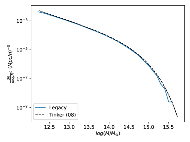
Figure 1: Mass function of dark matter halos in the Legacy simulation at redshift z=0. The mass function is consistent with the mass function fit presented in Tinker et al. (2008). All halos contain at least 20 dark matter particles.

In Figure 1 we shows the mass functions of the Legacy simulations used in this study. Over a mass range from $10^{12.2}-10^{15.5}$ M_⊙ the mass function is in good agreement with the fit proposed by Tinker et al. (2008). The latter has been matched against various different simulations by other groups and suggests that our simulations are consistent. In the following we will only consider halos with particle numbers $n\geq 20$ ( $\geq 1.086\times 10^{12}$ M_⊙) which corresponds to the mass range shown in the figure.

4 Results

We start this section by presenting results that confirm that the computation of the CMN from our simulations is consistent with the expected trends, before extending the analysis to estimate environmental dependencies.

4.1 Power Spectrum

The CMN is directly related to the shape of the power spectrum via Eqs. (13) and (12). In Figure 2 we show the input power spectrum from which the initial conditions of the simulations are generated, linearly extrapolated to $z=0$. The power spectrum measured from the simulation data at $z=0$ with the nbodykit software (Hand et al., 2018) is shown in the same figure as symbols with error bars. the errors are calculated using the estimator presented in Feldman et al. (1994) and Colombi et al. (2009) via:

$$\left(\frac{\Delta P}{P(k)}\right)^{2}=\frac{1}{C(k)}\left[1+\frac{2}{N_{p}P(k)}+\frac{1}{N_{p}^{2}P^{2}(k)}\right]$$ (15)

Where $C(k)$ is the number of statistically independent available wavenumbers, and $N_{p}$ the numbers of particles. The power spectrum of the simulation is in very good agreement with linear predictions for scales $\geq 5$ Mpc$/h$, but drops slightly, although still consistent within the errors, below the expectations at scales close to the simulation box sizes $>1000$ Mpc$/h$. On scales $<5$ Mpc$/h$ clear deviations from the linear power spectrum are found which are due to non-linear growth of structures. The derivation of the CMN starting from Eqs. (8) assumes linear growth of structure and hence is most applicable to the linear and mildly non-linear range of the power spectrum. We will therefore focus on CMNs on larger scales and smooth over scales of 5 Mpc$/h$ in the following sections.

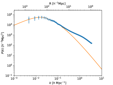
Figure 2: Input power spectrum used to generate the initial conditions for the simulation linearly extrapolated to $z=0$ (orange), and the power spectrum calculated from the simulation at $z=0$ (blue). Error bars show $1-\sigma$ errors. Deviations on small scales ($\leq 5\,\mathrm{Mpc}/h$, large $k$) are due to non-linear growth of structure. Overall the measured spectrum is in good agreement with the expectations from the input spectrum within errors.

4.2 The Global Cosmic Mach Number $\mathcal{M}_{g}$

4.2.1 Simulation Requirements

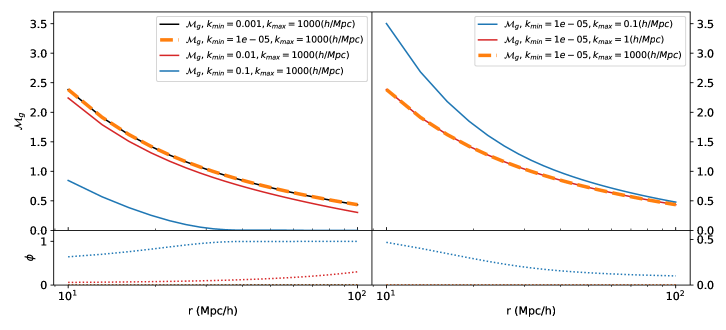
Figure 3: $\mathcal{M}_{g}$ as a function of the radius, for different upper and lower limits of the integration range of the power spectrum. This effectively truncates the power spectrum on one side or the other representing simulation volume and resolution limitations. Left: $\mathcal{M}_{g}$ as a function of $r$ for different $k_{min}$. $k_{max}$ has been set at $1000\,\mathrm{h/Mpc}$ . Right: $\mathcal{M}_{g}$ as a function of $r$ for different $k_{max}$. $k_{min}$ has been set, $10^{-5}\,h/\mathrm{Mpc}$. The solid/dashed lines are the results for different ranges of modes. The dotted lines in the bottom panel show the relative difference, compared to the case taking the full power spectrum from $k_{max}$ to $k_{min}$ corresponding to all modes on scales between $\sim 5\,\mathrm{Mpc}/h$ and $\sim 10^{3}\,\mathrm{Mpc}/h$. The black line, corresponding to $k_{min}=10^{-3}\sim h/$Mpc, is identical to the orange one, which confirms that, in $\Lambda$CDM, for $k_{min}\leq 10^{-3}\sim h/$Mpc results for the CMNs converge. The bottom panel shows the residual ${\phi=\frac{\mathcal{M}_{\mathrm{full}}-\mathcal{M}_{\mathrm{truncated}}}{\mathcal{M}_{\mathrm{full}}}}$ , the relative error between the results from the initial full spectrum (orange dashed line) and those from the truncated spectra.

In this section we will quantify the intrinsic errors in the calculation of the global Mach number depending on the simulation setup and show that the Legacy simulation used here minimises such errors. The CMN depends on the power spectrum across many scales, but all scales do not contain the same power. As numerical simulations cover the power spectrum only on scales from the Nyquist frequency of the simulation setup up to the size of the simulation volume, one expects this to affect CMNs measured in simulations. Too coarse resolution will result in an underestimate of the velocity dispersion $\sigma$ due to missing small scale power, and a simulation volume not covering to large enough scales will result in an underestimate of the bulk flow $u$. Figure 3 shows the global Mach numbers as predicted analytically using different integration limits $k_{\mathrm{min}}$ and $k_{\mathrm{max}}$ for the theoretical input power spectrum, mimicking different simulation setups. As expected, increasing the lower limit $k_{\mathrm{min}}$, and therefore ignoring large-scale modes, result in lower Mach numbers, as these large modes contribute to the bulk flow. Eventually, the Mach number will tend towards zero, once $k_{\mathrm{min}}\sim 1/r$ corresponding to the size of the region over which the CMN is calculated. Similarly, lowering $k_{\mathrm{max}}$ results in higher Mach numbers, as fewer small scales are resolved and contribute to the velocity dispersion. However, the relation between the Mach number and the power spectrum strictly only holds in the linear regime, so increasing the resolution will not change the Mach numbers measured at redshift zero, as the contributions on scales smaller than $\sim 5\,\mathrm{Mpc}/h$ are smoothed over in our approach. A higher resolution might be useful when measuring $\mathcal{M}$ at a larger redshift with a smaller smoothing scales, when non-linearities are still confined to small scales. Based on Fig. 3 constraints on CMNs with accuracy better than $10\%$ are only achieved for simulations that include modes up to scales of $1000\,\mathrm{Mpc}/h$, and at least resolve all scales in the linear regime (i.e. larger than $\sim 5\,\mathrm{Mpc}/h$). Mach numbers computed with the full input power spectrum from $k_{\mathrm{min}}=10^{-5}\,h/\mathrm{Mpc}$ to $k_{\mathrm{max}}=1000\,h/\mathrm{Mpc}$ are identical to those calculated with parameters consistent with the full box size of the Legacy simulation, supporting the notion that our simulation volume in this study is large enough to capture all relevant scales and to predict accurate Mach numbers. Present state-of-the-art cosmological hydrodynamics simulations like e.g. The Eagle (Crain et al., 2015; Schaye et al., 2015) or Illustris (Springel et al., 2018) use volumes of a few hundred $\,\mathrm{Mpc}/h$ on the side. Therefore, one would expect CMNs calculated using these simulations to be $\sim 5\%$ smaller than what they should be on scales of $\sim 10\,\mathrm{Mpc}/h$, and $\sim 30\%$ smaller at scales of a $\sim 100\,\mathrm{Mpc}/h$.

4.2.2 The CMN as a function of scale

We here show the distribution of global CMN, calculated as the average CMN of 50 randomly placed non-overlapping spheres in the simulation volume using Eq. (5).

Figure 4 shows the distribution of 500 global CMNs, calculated each averaging over 50 spheres of radius $R=10,\,20\,$ and $40\,\mathrm{Mpc}/h$, respectively. The distributions are well described by Gaussians. As the radius increases, both the average and width of the distributions decrease reflecting the shape of the power spectrum and the increase in homogeneity of the universe averaging over larger scales, respectively.

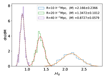
Figure 4: Distribution of the CMN for spheres of radius $10$, $20$, and $40\,\mathrm{Mpc}/h$. The distributions are well fitted by Gaussian distributions (dashed lines).

Figure 5 shows the predicted CMN from the simulation for radii $R=10-100\,\mathrm{Mpc}/h$. In order to compare with the theoretical expectations, CMNs were calculated using Equations (12) and (13) by integrating the extrapolated input power spectra shown in Figure 2, with smoothing applied over $r_{s}=5\,\mathrm{Mpc}/h$ for both simulation data and theoretical predictions, as discussed in section 2. The power spectrum was smoothed using a Gaussian filter and the simulation data using cubes, but as noted by Suto et al. (1992) and also seen in our own tests, the actual shape of the smoothing function is not as important as the smoothing scale.

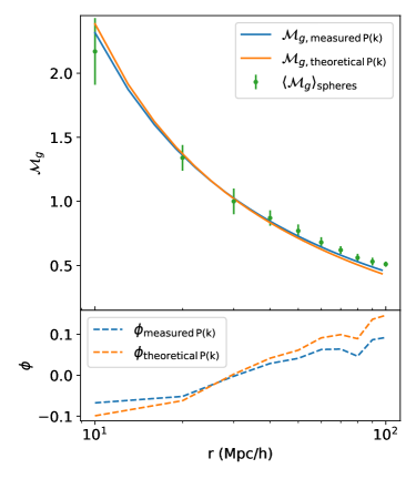
Figure 5: The global CMN as a function of radius. The orange and blue solid lines show the results inferred from the theoretical input and measured power spectra, respectively, integrating Eqs. (13) and (12). The green points are calculated using the halos in the simulation (100 groups of 50 spheres at each radius). All results were obtained using a $5\,\mathrm{Mpc}/h$ smoothing length. Error bars are standard deviations around the mean value. The bottom panel shows the relative error between the results from the spectra and those from the spheres, e.g $\phi_{\mathrm{measured\,P(k)}}=\frac{\langle\mathcal{M}_{g}\rangle_{\mathrm{spheres}}-\mathcal{M}_{g,\mathrm{measured\,P(k)}}}{\mathcal{M}_{g,\mathrm{spheres}}}$

The orange solid line of Figure 5 shows CMNs obtained by integrating the theoretical power spectrum, while the blue line shows the results integrating the measured power spectrum (the orange and blue spectra of Figure 2, respectively ) from $r=10$ to $100\,\mathrm{Mpc}/h$ in Eq. (12) and (13). The green points are obtained by calculating the average $\left<\mathcal{M}_{g}\right>$ over a hundred $\mathcal{M}_{g}$. The latter are averaged over $50$ spheres at each radius. Error bars are the standard deviation around the average $\left<\mathcal{M}_{g}\right>$. There is a small disagreement between the results using the theoretical input spectrum versus the measured one, which is a consequence in the slight difference in the power spectra shown in Figure 2, which lies within the errors of the measured spectrum. At small scales, $\mathcal{M}_{g}$ obtained from averaging spheres match the predictions quite well, but as scales increases, a small discrepancy starts to appear, as the measured average value $\left<\mathcal{M}_{g}\right>$ (green points) lie systematically above the expected values from integrating the power spectra.

We do not expect this deviation to be due to the smoothing scale. We confirm this in Appendix A by changing the smoothing scales $r_{s}$ systematically and finding the same deviation. A possible explanation for the deviation is that linear theory underestimates the bulk flow of structure as seen in the velocities of clusters (Colberg et al., 2000; Sheth & Diaferio, 2001; Cen et al., 1994). Further support for the notion of this being related to the build-up of large scale structure in the cosmic web comes in section 4.2.4 in which we show that these deviations on large scales are systematically reduced going to higher redshift when structures on these scales are still not well developed. Deviations are also expected to some extent given that halos are not perfect tracers of the underlying matter density field. As we show in Appendix A our results improve if all dark matter particles within a region are taken into account. However, we will continue to calculate CMNs using halos in this study and not dark matter particles to allow the connection to observations which rely on galaxies whose movements follow closely those of their hosting dark matter halos. In general, the agreement between all three methods shown in Fig. 5 is good, with a maximum deviation of the measured $\left<\mathcal{M}_{g}\right>$ at scales of $\sim 100\,\mathrm{Mpc}/h$ that leads to an error of $\sim 10\%$. As presented in section 4.2.4, our results indicate that this deviation disappears at higher redshift, when non-linearities on small large scale are not developed yet.

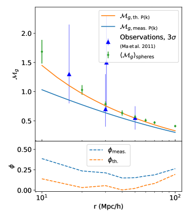
Figure 6: $\mathcal{M}_{g}$ vs $r$ without smoothing on scales smaller than $r_{s}=5$ Mpc$/h$. Coincidentally, the simulation results overlap with calculations using the linear input power spectrum of the simulation (orange line), while they are offset with regards to the calculations using the actual power spectrum of the simulation (blue line). The blue triangles represent the results from observations (obtained without smoothing) presented in Ma et al. (2011). Like on the previous figure, the residuals on the bottom panel are calculated via e.g $\phi_{\mathrm{meas.\,P(k)}}=\frac{\langle\mathcal{M}_{g}\rangle_{\mathrm{spheres}}-\mathcal{M}_{g,\mathrm{meas.\,P(k)}}}{\mathcal{M}_{g,\mathrm{spheres}}}$ We show that the CMNs calculated using halos are consistent with observations, but they are significantly larger than the results obtained from the measured spectrum, highlighting the need to smooth over non-linearities.

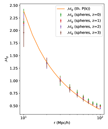
Figure 7: $\mathcal{M}_{g}$ as a function of radius, for redshift 0 to 3. High redshift points are consistent with the theoretical spectrum, as non linearities develop later. All results were obtained using a $5\,\mathrm{Mpc}/h$ smoothing length.

4.2.3 Impact of non-linearities

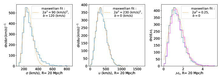
Figure 8: Distributions of $u$,$\sigma$, and $\mathcal{M}$, for 4000 realizations, fitted with distributions of the form $P(x)=\sqrt{\frac{2}{\pi}}\frac{(x-b)^{2}e^{(x-b)^{2}/2a^{2}}}{a^{3}}$.The magenta dashed histogram in the third panel shows the results of a Monte-Carlo simulation of the CMN based on randomly choosing values for $u$ and $\sigma$ from the fitted distribution shown in the two left most panels.

The main assumption in the derivation of the CMN is that linear theory holds on scales of interest. While it should do so also in the mildly non-linear regime, it is interesting to gauge the impact of non-linear structure on the estimates of the CMN on different scales. As we have shown in Fig. 2 the power spectrum deviates on scales $<5~{}$Mpc$/h$ from the linear extrapolation. As a consequence smoothing is applied over these scales in simulations as well as in observations (Ostriker & Suto, 1990). Figure 6 shows our results if we do not apply any smoothing in the calculation of $\mathcal{M}_{g}$ for the same three methods we applied in the previous section, i.e. the CMNs calculated with the theoretical and measured spectra, and using the halos. The Mach numbers calculated with the measured spectrum (including non-linearities) using linear theory lie below those found with the theoretical input spectrum linearly extrapolated to $z=0$, as the non-linearities cause an increase in power on small scales and result in a generally larger velocity dispersion $\sigma$. The Mach numbers calculated using our simulated halos deviate from the other estimates.The maximum deviation appears on scales of $\sim 10\,\mathrm{Mpc}/h$ where there is a $\sim 18\%$ difference between the results of the halos and the results of the theoretical input spectrum. This increases to $\sim 40\%$ for the measured spectrum. On large scales, the results from the halos and the theoretical input spectrum overlap and are off-set compared to those of the measured spectrum, which includes significant excess power due to non-linearities. The agreement between $\mathcal{M}_{g}$ derived from halos with the theoretical one is most likely coincidence, as linear theory, which connects the CMN calculated in real space with the spectrum integration, only holds if the non-linearities are not too large . These results confirm that extending linear calculations for $\mathcal{M}_{g}$ to the non-linear regime is not as straightforward as simply using the full non-linear power spectrum. For completeness, we also compare $\mathcal{M}_{g}$ obtained from halos in the simulation to observations (both without smoothing) presented in Ma et al. (2011), which reveals good agreement within albeit large uncertainties of the observations. Future surveys will be key to significantly reduce uncertainties in observations and provide stronger constraining power.

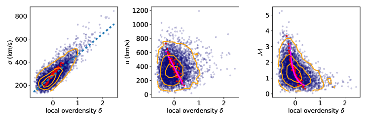
Figure 9: Blue points: local $\sigma$, $u$, and $\mathcal{M}_{l}$ for individual halos, as functions of the overdensity $\delta$ enclosed in the corresponding spheres, for 4000 random spheres of radius 20 Mpc$/h$. The contours show the regions where the distribution lie above $5\%$,   $33\%$, and $66\%$ of its maximum, respectively. $\sigma$ is correlated with $\delta$, while $u$ does not show any strong trend, as a consequence $\mathcal{M}$ is a decreasing function of the overdensity. The blue dashed line shows the best linear fit for $\sigma$. Red points: Same for the rank ordered global Mach numbers $\hat{\mathcal{M}}_{g}$, averaged over groups of 50 spheres of similar local Mach numbers $\mathcal{M}_{l}$. The averaged bulk flow $u$ now depends clearly on the averaged overdensity $\delta$ while no such trend is visible in the local values (blue points).The magenta dotted lines shows the best fit for $\hat{\mathcal{M}}_{g}$ with the form $\hat{\mathcal{M}}_{g}=\frac{1}{\alpha+\beta\delta}$, with $\alpha=0.895$ and $\beta=2.68$ , as well as the best linear fit for the global ranked bulk flow $u=A\delta+B$ with $A=-680,B=389$.

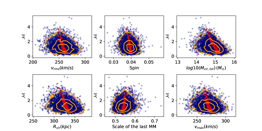
Figure 10: $\mathcal{M}_{l}$ (blue points) as a function of average halo properties of halos contained in spheres of radius $20~{}{\mathrm{M}pc}/h$. The studied properties are: spin, virial radius $R_{vir}$, velocity dispersion $v_{rms}$, maximum circular velocity $v_{max}$, scale of the last major merger. $M_{l}$ shows a broadening of the the total Mass distribution going to smaller values. The rank ordered global Mach number$\hat{\mathcal{M}}_{g}$ (red points) shows tight correlations with halo properties (see section 4.4 for more details on $\hat{\mathcal{M}}_{g}$).

4.2.4 Evolution with redshift

The global CMN by construction does not show any redshift dependency, as both $u$ and $\sigma$ scale with the power spectrum similarly see Eq. (12) and (13). If anything, the Mach numbers calculated with dark matter halos should match more accurately the theoretical predictions at higher redshift, when non-linearities have not appeared yet. The scale at which non-linearities kick in decreases with redshift thus suggesting that the CMN provides a more accurate measure of the power spectrum at smaller scales at high redshift.

In Figure 7 we show $\mathcal{M}_{g}$ as a function of radius for different redshift $z$ as well as the results obtained doing the theoretical calculation from the corresponding power spectra, measured in the simulation. First, we see that the results at $z>0$ agree with those at $z=0$. This is the case both for the results measured from spheres in the simulation volume, and for those obtained by integrating the power spectrum. We also notice that the agreement between the measured $\mathcal{M}_{g}$ and the theoretical predictions does get better at higher redshift. The differences between the results at $z=0$ and those at $z>0$ come solely from the non-linearities that appear as redshift decreases.

4.3 The local Cosmic Mach Number $\mathcal{M}_{l}$

As shown on Figure 4, the distributions of the CMNs are fairly wide. Given the relation of $\mathcal{M}_{g}$ with the matter power spectrum, which describes the density fluctuations of the Universe, the difference between the Mach numbers at a given scale are expected to arise from differences in the "local" environment on scales over which halos are averaged. In the following sections, we investigate potential links between the Mach number of a single region and the properties of the region over which we average including their environment. The Mach numbers $\mathcal{M}_{g}$ presented so far are obtained from averaging over a large number of randomly chosen non-overlapping spheres on a given scale $r$, in effect averaging over variations in, $u$ and $\sigma$, and their dependence on physical properties. To investigate physical connections more directly we calculate an alternative Mach number which does not rely on ensemble averaging. We will calculate the local Mach number $\mathcal{M}_{l}$ for individual spheres as the ratio of the bulk flow and the velocity dispersion of halos inside said spheres in contrast to the global Mach number $\mathcal{M}_{g}$ which is computed using many such spheres. Note that $\mathcal{M}_{g}\equiv\left<u\right>/\left<\sigma\right>$ is by construction not the average of $\mathcal{M}_{l}=u/\sigma$ for individual spheres. The local nature of $\mathcal{M}_{l}$ trades the clear connection to the power spectrum of the simulation for, potentially, more straightforward relations to environmental physical properties. In the following, $\mathcal{M}_{l}$ will be explored.

Figure 8 shows the distributions of the bulk flow $u$, the velocity dispersion $\sigma$, and the local Mach number $\mathcal{M}_{l}$, for one thousand spheres of radius $20\,\mathrm{Mpc}/h$ . The bulk flow is well described by a Maxwellian distribution. Each component of the average velocity of the group of halos in a sphere follows a Gaussian distribution so the bulk flow of the group follows a Maxwellian distribution (Kumar et al., 2015). The velocity dispersion does not follow a Maxwellian distribution as closely as the bulk flow, as it shows some excess at the large $\sigma$ tail, but the discrepancy is not large. The velocity dispersion is however closer to a Maxwellian distribution than the results shown by Nagamine et al. (2001). The difference can be attributed to the smoothing of non-linear small-scale fluctuations which has been omitted in Nagamine et al. (2001). The Mach number is well described by a Maxwellian distribution too, in agreement with previous findings (Nagamine et al., 2001). Randomly choosing $u$ and $\sigma$ values using their respective distributions and calculating $\mathcal{M}_{l}$ produce the green dashed histogram in the third panel, which agrees very well with the measured distribution of $\mathcal{M}_{l}$ in the simulation. This confirms that $u$ and $\sigma$ can be considered independent variables which is a feature of Gaussian random density fields, where modes on different scales are independent of each other.

Since the definition of $\mathcal{M}_{l}$ relies only on dynamical properties of a system of halos, and dark matter dynamics are primarily driven by the the density field, we expect the Mach number to show correlations with density estimates of the local environment and its vicinity. Figure 9 shows for 4000 spheres of radius $20\,\mathrm{Mpc}/h$ $\mathcal{M}_{l}$, $u$, and $\sigma$, against the overdensity $\delta=\frac{\rho-\rho_{m}}{\rho_{m}}$, with $\rho$ as the density in a sphere and $\rho_{m}$ the average density in the Universe. The density $\rho$ is calculated using all the dark matter particles in the relevant region, not only those associated with dark matter halos. While the bulk flow shows no clear correlation with the overdensity, the velocity dispersion seems to be linearly related with it. As a result, $\mathcal{M}_{l}$ is a decreasing function of overdensity.

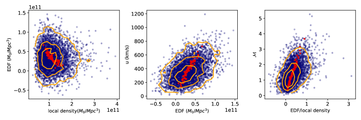
Figure 11: Left: Environmental density fluctuation (EDF) between two nearby, diametrically opposed $60\,\mathrm{Mpc}/h$ spheres vs local density in a 20 $\,\mathrm{Mpc}/h$ sphere, for 4000 realizations. Center: $u$ vs EDF, the panel shows a positive correlation, which is expected due the relation between $u$ and the density gradient in the region. Right: $\mathcal{M}_{l}$ vs the ratio of EDF to local density. $u$ depends on the EDF, which is a measure of the large scale density gradient. The EDF and $\delta$ are uncorrelated, so $\mathcal{M}_{l}$ is also a measure of their ratio. Blue shows local values, while red is for rank ordered global CMN $\hat{\mathcal{M}}_{g}$ obtained from averaging in groups of spheres of similar local Mach numbers (see section 4.4 for more details). In addition to the relations with local values, we observe a strong correlation between $\delta$ and the EDF, which causes the relation between the global $u$ and $\delta$ seen in Figure 9.

The pair-wise velocity dispersion $\sigma_{12}(r)$, which is the dispersion of a pair of tracers separated by a distance $r$ shows a very similar trend. The Cosmic Virial Theorem predicts a relation between $\sigma_{12}$ and density, and this relation has been previously observed in N-body simulations (Strauss et al., 1998). It is therefore not surprising that the velocity dispersion of the groups exhibit a similar behavior. These results are overall consistent with those presented in Nagamine et al. (2001), even though the Legacy simulation includes significantly more large scale modes that are essential for the calculation of $u$, $\mathcal{M}$, and the overdensity, as shown in Figure 3. We also note that we do not find a clear correlation between $\delta$ and the bulk flow. As for $\mathcal{M}_{l}$ we find that the median of the distribution of overdensities $\delta$ systematically gets larger as $\mathcal{M}_{l}$ gets smaller with an increasing scatter. Our results predict that regions with $\mathcal{M}_{l}\leq 1$ have on average a matter densities corresponding to $\delta>0$. The latter is not surprising given the positive correlation of $\sigma$ with $\delta$ and the lack of a clear correlation of the bulk flow, but it also reflects the fact that more overdense regions are typically the dominant large scale gravitational sources in their environment and therefore do not show much bulk flow themselves but have mostly matter moving towards them. Halos in underdense regions like voids in contrast could either be moving with a large bulk velocity towards a more overdense region and hence show large $\mathcal{M}_{l}$ or still be in the process of getting accelerated.

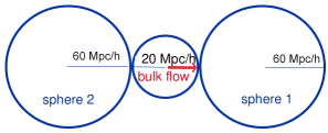
Figure 12: Definition of the environmental density fluctuation. Sphere 1 (2) is in the direction (opposite direction) of the bulk flow. The EDF is defined as the density difference between these two large spheres via $\eta_{{\mathrm{E}DF}}=\rho_{1}-\rho_{2}$.

Figure 10 shows $\mathcal{M}_{l}$ plotted against the average halo properties of the objects in 4000 spheres of radius $20\,\mathrm{Mpc}/h$, except for the virial mass $M_{\mathrm{vir}}$, which is the total of all halos, for the following properties: Spin, virial radius $R_{\mathrm{vir}}$, velocity dispersion $v_{\mathrm{rms}}$, maximum circular velocity $v_{\mathrm{max}}$, scale of the last major merger and spin .

$\mathcal{M}_{l}$ does not show any strong correlation with average halo properties, except for a weak correlation with the total mass of halos, which is a tracer of the underlying density field. We find similar trends also for the average velocity dispersion $v_{rms}$ and maximum circular velocity $v_{max}$, both of which are related to the total mass of halos in a region. Interestingly, the average last major merger halos in high $\mathcal{M}_{l}$ regions experience is slightly later than in low $\mathcal{M}_{l}$ regions although these regions can have individually last major mergers that happen later. The intrinsic scatter of the time of the average last major merger decreases with $\mathcal{M}_{l}$. The average spin parameter of halos show a very slight dependence on $\mathcal{M}_{l}$ in becoming somewhat smaller for larger $\mathcal{M}_{l}$.

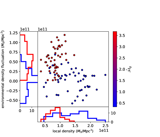
Figure 13: Main panel: same as the top left panel of 11 but showing the extreme groups (red : highest $\hat{\mathcal{M}}_{g}$; blue : lowest) Side panels: histograms of the density and EDF of each group.

The expectation is that a large scale bulk-flow of a region follows density fluctuations around that region that source gradients in the gravitational potential. To quantify this effect we calculate the density in two larger adjacent spheres, one in the direction of the bulk flow $\rho_{1}$, and one in the opposite direction $\rho_{2}$ (see Figure 12). We call the density difference between these two spheres $\eta_{\mathrm{EDF}}=\rho_{1}-\rho_{2}$ the environmental density fluctuation (EDF). The top right panel of Figure 11 shows how the bulk flow depends on the environmental density fluctuation. A positive correlation is clearly visible. This is explained by the fact that a large overdensity will attract our group of halos if its influence is not compensated by an overdensity in the opposite direction. However, the scatter is quite large ($\sigma_{{\mathrm{E}DF}}/\left\langle\eta_{{\mathrm{E}DF}}\right\rangle\sim 3$ for the $33\%$ contour), which can be explained by two factors. First, a single overdensity in a nearby region is only the simplest scenario, the two spheres are but a rough simplification of the often complex topology of the gravitational potential which drives the motion of a group of halos. Also, the environmental density fluctuation is only an approximation of the local density gradient in the direction of the bulk flow, and this gradient has been shown to strongly correlate with the bulk flow (Kumar et al., 2015). This large scatter results in cases of negative EDF for $\mathcal{M}_{l}$.

Since the velocity dispersion linearly depends on the local density, the local Mach number correlates tightly with the ratio of the environmental density fluctuation and the local density, as shown on the panel all to the right of Figure 11. The pair of large spheres do not overlap with the central small sphere in order to avoid any accidental correlation between the environmental density and the local density, as shown in Figure 12. Overall, Figure 11 shows a clear relation between the Mach number and the properties of the density field of that region.Alternative definitions of the local density gradient by Kumar et al. (2015) show similar results.

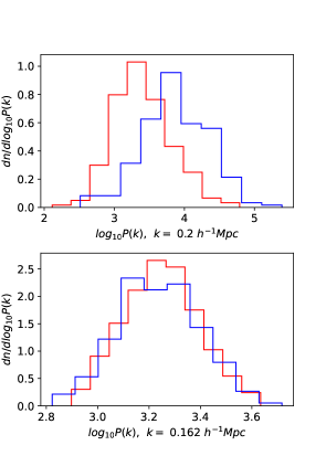
Figure 14: Distributions of the power of a small (top) and large (bottom) scale, for the 250 spheres with the highest (red) and lowest (blue) Mach numbers $\mathcal{M}_{l}$. The power on large scales is measured in a cube of side $120\,\mathrm{Mpc\,h^{-1}}$, around each sphere. The power of small-scale fluctuations is clearly correlated with the local CMN $\mathcal{M}_{l}$, but the large scale fluctuations are indistinguishable, suggesting the driver for the difference in $\mathcal{M}_{l}$ on a given scale is the velocity dispersion of halos on that scale.

Another way of looking at the relation between $\mathcal{M}_{l}$ and the environment is to look at the local power spectrum. We calculate the power spectrum of the density field in each sphere (corresponding to scales smaller than the radius) along with the power spectrum in a cube of $(120\,\mathrm{h^{-1}Mpc)^{3}}$ centered around the sphere, to measure the fluctuations on scales larger than the sphere. Figure 14 shows, for 250 spheres with the lowest local CMN $\mathcal{M}_{l}\sim 0.5$ (blue) and highest $\mathcal{M}_{l}\sim 3.5$ (red), the distribution of the value of the power spectrum for a typical large scale mode $k=0.2\,\mathrm{h/Mpc}$ (top panel) and small scale mode $k=0.162\,\mathrm{h/Mpc}$ (bottom panel). While the two histograms are almost identical for large sales, the distributions for small-scale fluctuations are clearly distinct, the power is typically larger for lower Mach numbers, as they typically have larger $\sigma$. The average large scale fluctuations do not seem to affect $\mathcal{M}_{l}$ as strongly as small scale modes, suggesting $\mathcal{M}_{l}$ is a good probe of the small scale power. These results show the same trend for all small and large modes we measured.

4.4 The rank ordered global Mach number

As we have shown in the previous section environmental effects are not easy discernible by measuring $\mathcal{M}_{l}$ for an individual sphere as they show large scatters around general trends. To overcome this limitation we here propose to enhance any potential signal in the data by stacking spheres of similar $\mathcal{M}_{l}$ and using them to calculate a rank ordered global CMN via $\hat{\mathcal{M}}_{g}\equiv\left<u\right>/\left<\sigma\right>$, where the average is taken over 50 spheres that are chosen to have similar local Mach numbers $\mathcal{M}_{l}$. The halo properties associated with these stacked spheres are calculated as the average of their value in each sphere of the stack. We focus on this ranked ordered Mach number instead of e.g. the average local Mach number, as $\hat{\mathcal{M}}_{g}$ can be connected to cosmology and the fluctuations of the power spectrum (see equations 12 & 13).

We use $4000$ non-overlapping spheres of the catalogs and sort them based on their local $\mathcal{M}_{l}$. Then, the $50$ spheres with the highest local Mach numbers are selected and used to calculate one global $\hat{\mathcal{M}}_{g}$, which is expected to be high. Another global $\hat{\mathcal{M}}_{g}$ is then calculated using the next $50$ spheres, and so on. Since spheres with a large $\mathcal{M}_{l}$ have a relatively large bulk flow and a small velocity dispersion we expect $\hat{\mathcal{M}}_{g}$ calculated based on these $\mathcal{M}_{l}$ to be large as well. By grouping spheres in this manner, the $\hat{\mathcal{M}}_{g}$ distribution covers a larger range in $\delta$ than the $\mathcal{M}_{g}$ distribution, as we force the creation of a number of extremely low and high $\hat{\mathcal{M}}_{g}$ values that would only rarely appear for $\mathcal{M}_{g}$ if the selection of spheres was kept fully random in the averaging process.

The red points of Figure 9 show the rank ordered Mach number $\hat{\mathcal{M}}_{g}$, $u$, and $\sigma$, obtained by the selection mentioned above. The linear relation between $\sigma$ and the local overdensity remains, but a new tight relation appears between $u$ and $\delta$. As a result, $\hat{\mathcal{M}}_{g}$ is now strongly correlated with $\delta$ and can be reasonably well fitted by a simple relation of the form $\hat{\mathcal{M}}_{g}=\frac{1}{\alpha+\beta\delta}$, with $\alpha=0.895$ and $\beta=2.68$.

The red points in Figure 10 show the relations between $\hat{\mathcal{M}}_{g}$ and halo properties. Again, the selection process and the grouping reveal a number of correlations that did not clearly appear with $\mathcal{M}_{l}$ (see Figure 10 blue points). The relation between $\hat{\mathcal{M}}_{g}$ and the total halo mass $M_{{\mathrm{v}ir,tot}}$ in the spheres, which is directly linked to $\delta$ is becoming much clearer. Because of the relation between $M_{{\mathrm{v}ir,tot}}$ and other halo properties, correlations with $\hat{\mathcal{M}}_{g}$ emerge. It is interesting to note that, when the global CMNs $\mathcal{M}_{g}$ are calculated using random spheres, they are likely to lie somewhere between $\sim 1$ and $\sim 1.5$, where the scatter is too large and erases most of the trends in the Figure. One particular interesting feature is the fact that $\hat{\mathcal{M}}_{g}$ increases with the average scale factor at which the last major merger took place. We observe later mergers in regions with a high Mach number. This would suggest that regions with a high Mach number (and therefore a low density) evolve more slowly than denser regions as is expected in the $\Lambda$CDM paradigm. We provide fits for the relations between $\hat{\mathcal{M}}_{g}$ and the halo properties in table 2.

The red points in Figure 11 show again results for $\hat{\mathcal{M}}_{g}$. The trends for $\mathcal{M}_{l}$ with $u$, and $\sigma$ are recovered although with much tighter scatter for $\hat{\mathcal{M}}_{g}$. However, a new clear anti-correlation between the environmental density fluctuation and the local density appears. This explains the trend seen in the red points of the middle panel of Figure 9. Since $u$ increases with the environmental density fluctuation, which appears to decrease with $\delta$, $u$ now decreases with $\delta$. As a result, $\hat{\mathcal{M}}_{g}$ is now a tight linear function of these different features of the density field. As such, it can be used as a proxy to measure them and extend the use of the CMN as a probe of structure formation in the Universe.

We highlight the impact of the rank ordering in Figure 13 which shows the environmental density fluctuation against the local density for the 4000 spheres of radius $20\,\mathrm{Mpc}/h$, presented in Figure 11,but color coded to represent the two groups of 50 spheres used to calculate the highest (red) and lowest (blue) global Mach numbers. The side panels show the histograms of $\delta$ and the EDF for each group. The trend shown in red on the first panel of Figure 11 is highlighted here by the selection process. Groups of high $\hat{\mathcal{M}}_{g}$ typically correspond to high EDF and low local densities, while lower $\hat{\mathcal{M}}_{g}$ lie lower on the figure, indicating a lower EDF. The average of the histograms changes with $\hat{\mathcal{M}}_{g}$, and the distributions of the bottom panel get wider as $\hat{\mathcal{M}}_{g}$ decreases. However, while there is a relation between the CMN and enclosed mass, we note that the shape of the mass function does not change significantly as $\mathcal{M}_{l}$ or $\hat{\mathcal{M}}_{g}$ increases.

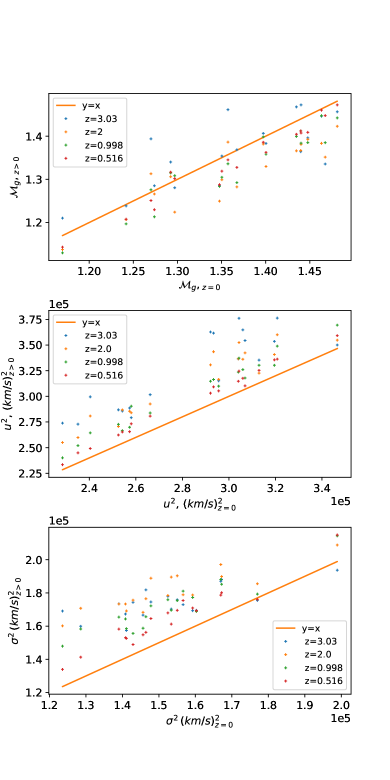
Figure 15: $\hat{\mathcal{M}}_{g},\,u^{2},\,\sigma^{2}$ for redshift 0 to 3, for rank ordered groups of spheres of $20\,\mathrm{Mpc}/h$. The same spheres were followed as $z$ increases. The values for the bulk flow and the dispersion have been linearly extrapolated to z=0. The high-z bulk flow is in good agreement with estimates at z=0, but the dispersions significantly differ at higher redshift, suggesting that we deviate from the linear regime at z=0 even after the smoothing.

To investigate further the impact of cosmic evolution on the CMN we use the rank ordered $\hat{\mathcal{M}}_{g}$ and follow the exact same co-moving spheres back in time and calculate their properties. Figure 15 show how $\hat{\mathcal{M}}_{g}$, and the corresponding linearly extrapolated $\sigma$ and $u$ evolve as $z$ increases. At $z=2$, the difference in $\hat{\mathcal{M}}_{g}$ can be as large as $20\%$ for high-$\hat{\mathcal{M}}_{g}$ groups, but is close to $5\%$ on average. In addition, the values of the linearly extrapolated bulk flow are consistent with the results at $z=0$, but linearly extrapolating $\sigma^{2}$ results in an overestimate of $\sim 20\%$ at $z=3$. This suggests that, although we smooth over non-linearities this does not fully remove them and that they still can impact results slightly, which complements the results shown on Figure 7. As $z$ decreases, non linearities develop. This mostly impacts the small-scale velocity fluctuations, and the difference between $\sigma(z>0)$ and $\sigma(z=0)$ increases as $z$ increases.

property	A	B
$v_{\mathrm{rms}}$	-0.073	20.00
Spin	-357.0	15.10
${\mathrm{log}}_{10}(M_{\mathrm{vir,tot}})$	-1.774	27.66
$R_{\mathrm{vir}}$	-0.047	16.67
scale factor of last major merger	34.71	-17.68
$v_{\mathrm{max}}$	-0.077	22.07

Table 2: Parameters used to fit $\hat{\mathcal{M}}_{g}$ to the halo properties with a linear function : $\hat{\mathcal{M}}_{g}=A\times\mathrm{property}+B$

5 Discussion and conclusion

In this work, we revisit the role of the Cosmic Mach Numberas a probe of the environment of halos introducing new measures. We have used a large scale cosmological N-body simulation from the Legacy project to calculate global Mach numbers for scales between $10$ and $100\,\mathrm{Mpc}/h$, comparing the theoretical predictions using the input power spectrum of the simulation and the power spectrum measured from the matter distribution in the simulation against Mach numbers calculated using halos found in the simulation. All these methods show good agreement when the density field is smoothed over non-linear scales of $5\,\mathrm{Mpc}/h$. We also highlight that smoothing the field and removing non-linearities is essential to achieve good agreement in the calculation of the CMN.

Including all dark matter particles in a region, and not just dark matter halos, improves the estimates of the CMN compared to theoretical expectation from $17\%$ to $10\%$ relative error and suggest intrinsic errors for estimates from galaxy surveys of the same level. We show that simulations are intrinsically limited in the accuracy they can achieve for the CMN based on the range of modes they include. Any simulation used to calculate Mach numbers with accuracy up to $\sim 10\%$ compared to theoretical predictions must include modes as large as $\sim 1000\,\mathrm{Mpc}/h$ and as small as $\sim 5\,\mathrm{Mpc}/h$ to accurately resolve all relevant scales. Present state-of-the-art simulations such as Eagle (Crain et al. (2015), Schaye et al. (2015)) or Illustris (Springel et al. (2018)) do resolve small scale-fluctuations, but consist of simulation volumes of a few hundred $\,\mathrm{Mpc}/h$, too small to include relevant large sale modes. Simulated CMN computed using these simulation may be $\sim 5\%$ too small at scales of $\sim 10\,\mathrm{Mpc}/h$, and up to $\sim 30\%$ too small at larger scales ($\sim 100\,\mathrm{Mpc}/h$), compared to expected results.

In addition, we study the relation between local Mach numbers and the properties of both the density field and the halos of a region. First, we corroborate the findings of previous studies, that the velocity dispersion strongly depends on the overdensity of the region and the bulk flow does not, which results in the local Mach number being a decreasing function of overdensity. Since dark matter halos act as tracers of the density field, it weakly correlates with the total halo mass within a region as well. We also show that the bulk flow of a sphere is positively correlated with the density difference between two diametrically opposed adjacent larger spheres $\eta_{\rm{EDF}}$, which acts as a measure of the density gradient of the region. The local CMN $\mathcal{M}_{l}$ thus provide a proxy of the relative strength of the density fluctuation measure $\eta_{\rm{EDF}}$ in contrast to the local density. The reason for these correlations seems to be two-fold. First, the relation between $u$ and $\eta_{\rm{EDF}}$ is clear, halos are drawn towards dense regions, especially if this attraction is not compensated by the action of another dense region in the opposite direction, hence this is why $u$ is correlated with the density gradient. Concerning $\sigma$, the velocity dispersion is conceptually similar to the pair-wise velocity dispersion $\sigma_{12}$, which is in turn closely linked to the local density by the Cosmic Virial Theorem. The regions we study are not virialized, but they are overdensities on their way towards eventual collapse and virialization. This suggests that $\sigma$ and $\sigma_{12}$ would behave in similar ways. We also show that the local Mach numbers are qualitatively consistent with the power spectra in that region.

While the local Mach number shows a correlation that has a large scatter with $\eta_{\rm{EDF}}$ it does not show strong correlations with local environmental measures or average halo properties. Therefore, we introduce a new quantity, the rank ordered global Mach number $\hat{\mathcal{M}}_{g}$ by grouping spheres of similar local Mach numbers together and use them to calculate the global cosmic Mach number instead of using a random sample of regions.

$\hat{\mathcal{M}}_{g}$ shows strong empirical correlations with many halo properties, such as total mass, average radius and velocity dispersion, for which we provide fits in Section 2, as well as with the local density and the environmental density fluctuation. Grouping the spheres in that manner also reveals a correlation between the enclosed density and $\eta_{\rm{EDF}}$.

The impact of non-linearities can be seen in the deviation of $\mathcal{M}_{g}$ from expectations based on the linear extrapolated power spectrum. While at low redshift we find deviations from the theoretical predicted CMNs for spheres with $r>40$ Mpc these vanish at $z\geq 3$ when the power spectrum on all scales follows the linearly extrapolated one. As shown in appendix B, our findings also suggest that focusing solely on massive objects does not significantly alter the derived global Mach numbers. We studied the effect of focusing on halos more massive than $10^{12.5}\,M_{\odot}$ and $10^{13}\,M_{\odot}$, and find the average CMN to be within 2 % and 8 %, respectively, of the value obtained using all halos above $10^{12.2}M_{\odot}$.

The results presented in this paper are the first part of a study exploring the suitability of the CMN as an environment probe. While we here focus on the exploration of N-body simulations, further studies will focus on the observational viability as well as on the comparison to other common environment measures. However, our results suggest that from an observational point of view the most efficient strategy to derive environmental information using the CMN on a given scale would be to group regions of similar local CMN $\mathcal{M}_{l}$ together for the calculation of their rank ordered $\hat{\mathcal{M}}_{g}$ and use such grouped spheres to investigate environmental effects of structure formation on the galaxy population. The grouping of spheres with similar $\mathcal{M}_{l}$ will allow to enhance underlying correlations and allow the efficient use of peculiar velocity surveys such as 6DFGS, the SDSS peculiar velocity catalogs. Studies based on the CMN will serve as a complementary approach to classic environment measures based on e.g. number densities and have the potential to be more robust given the weak dependence on survey depths compared to number density studies. In a future study we plan to investigate correlations between the CMN and classic environmental measure in more detail, as well as extend this work to galaxies instead of halos.

6 Acknowledgements

The Legacy simulations presented here were run on ARCHER and Cirrus hosted by EPCC. SK is grateful for support from the UK STFC via grant ST/V000594/1.’

7 Data availability

The data underlying this article will be shared on reasonable request to the corresponding author.

Appendix A Impact of smoothing scales and averaging procedure

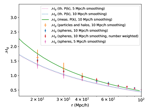
Figure 16: $\mathcal{M}_{g}$ vs $R$, for different smoothing lengths and averaging methods. Using the masses as weights does not seem to significantly impact the results, as the blue and red points overlap. The Mach numbers calculated with halos are consistent with theoretical predictions when the smoothing length $r_{s}$ is set to $5\,\mathrm{Mpc}/h$, but lie consistently lower when $r_{s}$ is increased to $10\,\mathrm{Mpc}/h$.

We here discuss the impact of smoothing non-linearities on various scales and the used averaging procedure on the predicted CMNs. Figure 16 shows measures of the Mach number following the same smoothing procedure with a smoothing length of $10\,\mathrm{Mpc}/h$ instead of the fiducial $5\,\mathrm{Mpc}/h$. We also show results calculated with a smoothing length of $10\,\mathrm{Mpc}/h$ and where the halos are averaged by number (we use $w_{i}=1$ in Equation 10 ). While the theoretical and measured Mach numbers are in good agreement at small scales when the field is smoothed over $5\,\mathrm{Mpc}/h$, a significant discrepancy appears when using a $10\,\mathrm{Mpc}/h$ smoothing length. The averaging method does not seem to matter, as the results from the mass-weighted and number-weighted (see Equation (9)) procedures are almost identical. A possible explanation for the observed discrepancy is that halos are not perfect tracers of the density field. To test this, we perform the calculation of M using both the halos and all the dark matter particles that do not belong in a halo within a sphere. We here show the results calculated with 10 groups of 10 spheres. Including particles greatly increases the computation time, so the sample size was decreased. This seems to improve our results at low scale (even though it would benefit from an increased sample size), as we more efficiently capture the density modes with the particles. The amplitude of the effect seems to increase with the smoothing scale, as the particles are not needed for consistent results with a $5\,\mathrm{Mpc}/h$ smoothing scale. Indeed, by using the particles, we can measure Mach numbers that are consistent with those predicted by the measured power spectrum. However, in this study, we calculate CMNs with dark matter halos since observations focus on galaxies, which reside in halos. We note that there is a $\sim 10\%$ discrepancy between the results using halos only and those also including particles at scales $\lesssim 30\,\mathrm{Mpc}/h$, for a smoothing length of $10\,\mathrm{Mpc}/h$.

Appendix B Effects of sample selection

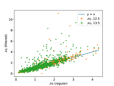
Figure 17: The local Mach numbers $\mathcal{M}_{l}$ calculated using only halos more massive than $10^{12.5}\,M_{\odot}$ (orange points) or than $10^{13}\,M_{\odot}$ (green points) vs $\mathcal{M}_{l}$ calculated with all resolved halos. The CMN calculated without the small halo are on average slightly larger than the actual CMN, with some rare rare points reaching significantly higher values. Although $\gtrsim 55\%$ ($\gtrsim 85\%$) of the halos are lighter than $10^{12.5}\,M_{\odot}$ ($10^{13}\,M_{\odot}$), the impact on the final global ranked Mach number is small (2% and 8% on average) .

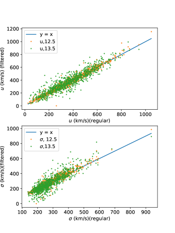
Figure 18: Similar to 17, but for $u$ (top) and $\sigma$ (bottom). On average, $u$ and $\sigma$ are not significantly affected by the mass filter, but the some dispersion are reduced to very small values, causing a large overestimate of the corresponding CMN.

Observational surveys have completeness limits based on their depth. To model the impact on the CMN we here apply mass cuts to halos in our simulation volume. Figure 17 shows $\mathcal{M}_{l}$ calculated after filtering out all halos less massive than $10^{12.5}\,M_{\odot}$ (orange) or $10^{13}\,M_{\odot}$ (green) plotted against $\mathcal{M}_{l}$ without mass cut for the same group of spheres. We see that most Mach numbers remain virtually unchanged, which is of interest for observational measures of $\mathcal{M}_{l}$. This also suggests that the small halos, (which on average account for $\sim 55\%$ of the total number of halos in these $20\,\mathrm{Mpc}/h$ spheres for the $10^{12.5}\,M_{\odot}$ filter and $\sim 85\%$ for the $10^{13}\,M_{\odot}$ filter), are not the main drivers of $\mathcal{M}_{l}$. In the terms of the CMN massive halos are therefore accurate tracers of the underlying velocity fields and the associated matter power spectrum. First, the average $\mathcal{M}_{l}$ is overestimated by 2% (8%) when using the $10^{12.5}\,M_{\odot}$ ($10^{13}\,M_{\odot}$) filter. Some CMNs reach extremely high values when calculated without the lighter halos : up to ten times the average. These come from spheres where the dispersion has been reduced to very small values (of the order of a dozen km/s), as only few, very massive objects remain in the region.

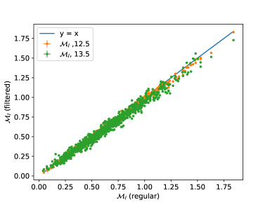
Figure 19: Similar to 17, but for spheres of $60\,\mathrm{Mpc}/h$. With such large spheres, no extremely high $\mathcal{M}_{l}$ can be seen, but $\mathcal{M}_{l}$ tends to decrease by a few $\%$ as the lighter halos are removed.

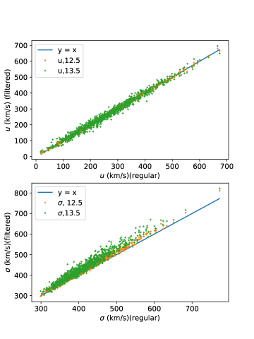
Figure 20: Similar to 18, but for spheres of $60\,\mathrm{Mpc}/h$. $u$ suffers no systematic changes as the mass cut increases, but $\sigma$ tends to be overestimated by up to $10\%$ when only keeping halos more massive than $13.5M_{\odot}$.

We note that this average systematic effect is smaller than the statistical dispersion around the average values of the CMN presented in Figure 5, and therefore do not invalidate the conclusions drawn from it. Also, this systematic effect seem to disappear at larger radii, as we show in figures 19 and 20. As few spheres are left with very small dispersion and few objects, no Mach numbers reach abnormally high values. However, they tend to decrease as the mass limit increases. Using only the most massive halos result in an overestimate of $\sim 10$ % of the velocity dispersion, while no systematic change can be detected in $u$. This shows that smaller halos tend to more accurately follow the bulk flow formed by larger halos, which do not correctly represent the small scale fluctuations of the velocity field. Once more, this effect is roughly as strong as the observed scatter and is not likely to alter the conclusions of the previous sections.

References

- Agarwal & Feldman (2013) Agarwal S., Feldman H. A., 2013, MNRAS, 432, 307
- Bartlett & Blanchard (1996) Bartlett J. G., Blanchard A., 1996, A&A, 307, 1
- Behroozi et al. (2013) Behroozi P. S., Wechsler R. H., Wu H.-Y., 2013, ApJ, 762, 109
- Cen et al. (1994) Cen R., Bahcall N. A., Gramann M., 1994, ApJ, 437, L51
- Colberg et al. (2000) Colberg J. M., White S. D. M., MacFarland T. J., Jenkins A., Pearce F. R., Frenk C. S., Thomas P. A., Couchman H. M. P., 2000, MNRAS, 313, 229
- Colombi et al. (2009) Colombi S., Jaffe A., Novikov D., Pichon C., 2009, MNRAS, 393, 511
- Crain et al. (2015) Crain R. A., et al., 2015, MNRAS, 450, 1937
- Davis et al. (1985a) Davis M., Efstathiou G., Frenk C. S., White S. D. M., 1985a, ApJ, 292, 371
- Davis et al. (1985b) Davis M., Efstathiou G., Frenk C. S., White S. D. M., 1985b, ApJ, 292, 371
- Feldman et al. (1994) Feldman H. A., Kaiser N., Peacock J. A., 1994, ApJ, 426, 23
- Hahn & Abel (2011) Hahn O., Abel T., 2011, MNRAS, 415, 2101
- Hand et al. (2018) Hand N., Feng Y., Beutler F., Li Y., Modi C., Seljak U., Slepian Z., 2018, Astron. J., 156, 160
- Hinshaw et al. (2013) Hinshaw G., et al., 2013, ApJS, 208, 19
- Kumar et al. (2015) Kumar A. N., Wang Y., Feldman H. A., Watkins R. J., 2015, Bulletin of the American Physical Society, 2016
- Linder (2005) Linder E. V., 2005, Phys. Rev. D, 72, 043529
- Ma et al. (2011) Ma Y.-Z., Ostriker J., Zhao G.-B., 2011, Journal of Cosmology and Astroparticle Physics, 2012
- Nagamine et al. (2001) Nagamine K., Ostriker J. P., Cen R., 2001, ApJ, 553, 513
- Ostriker & Suto (1990) Ostriker J. P., Suto Y., 1990, ApJ, 348, 378
- Peebles (1980) Peebles P. J. E., 1980, The large-scale structure of the universe
- Planck Collaboration et al. (2020) Planck Collaboration et al., 2020, A&A, 641, A6
- Schaye et al. (2015) Schaye J., et al., 2015, MNRAS, 446, 521
- Sheth & Diaferio (2001) Sheth R. K., Diaferio A., 2001, Monthly Notices of the Royal Astronomical Society, 322, 901
- Springel (2005) Springel V., 2005, Mon. Not. Roy. Astron. Soc., 364, 1105
- Springel et al. (2005) Springel V., et al., 2005, Nature, 435, 629
- Springel et al. (2018) Springel V., et al., 2018, MNRAS, 475, 676
- Springel et al. (2020) Springel V., Pakmor R., Zier O., Reinecke M., 2020, arXiv e-prints, p. arXiv:2010.03567
- Strauss et al. (1993) Strauss M. A., Cen R., Ostriker J. P., 1993, ApJ, 408, 389
- Strauss et al. (1998) Strauss M. A., Ostriker J. P., Cen R., 1998, Astrophys. J., 494, 20
- Suto et al. (1992) Suto Y., Cen R., Ostriker J. P., 1992, ApJ, 395, 1
- Tinker et al. (2008) Tinker J., Kravtsov A. V., Klypin A., Abazajian K., Warren M., Yepes G., Gottlöber S., Holz D. E., 2008, ApJ, 688, 709
- Turner (1997) Turner M. S., 1997, arXiv e-prints, pp astro–ph/9703161
- Vikhlinin et al. (2009) Vikhlinin A., et al., 2009, ApJ, 692, 1060
- Weinberg (2008) Weinberg S., 2008, Cosmology. Oxford University Press