An Improved Analysis of Gradient Tracking
for Decentralized Machine Learning

Anastasia Koloskova
EPFL
anastasia.koloskova@epfl.ch &Tao Lin
EPFL
tao.lin@epfl.ch &Sebastian U. Stich
EPFL
sebastian.stich@epfl.ch
Current affiliation: CISPA Helmholtz Center for Information Security.
Abstract

We consider decentralized machine learning over a network where the training data is distributed across n𝑛n agents, each of which can compute stochastic model updates on their local data. The agent’s common goal is to find a model that minimizes the average of all local loss functions. While gradient tracking (GT) algorithms can overcome a key challenge, namely accounting for differences between workers’ local data distributions, the known convergence rates for GT algorithms are not optimal with respect to their dependence on the mixing parameter p𝑝p (related to the spectral gap of the connectivity matrix).
We provide a tighter analysis of the GT method in the stochastic strongly convex, convex and non-convex settings. We improve the dependency on p𝑝p from 𝒪(p2)𝒪superscript𝑝2\mathcal{O}(p^{-2}) to 𝒪(p1c1)𝒪superscript𝑝1superscript𝑐1\mathcal{O}(p^{-1}c^{-1}) in the noiseless case and from 𝒪(p3/2)𝒪superscript𝑝32\mathcal{O}(p^{-3/2}) to 𝒪(p1/2c1)𝒪superscript𝑝12superscript𝑐1\mathcal{O}(p^{-1/2}c^{-1}) in the general stochastic case, where cp𝑐𝑝c\geq p is related to the negative eigenvalues of the connectivity matrix (and is a constant in most practical applications). This improvement was possible due to a new proof technique which could be of independent interest.

1 Introduction

Methods that train machine learning models on decentralized data offer many advantages over traditional centralized approaches in core aspects such as data ownership, privacy, fault tolerance and scalability [12, 33]. Many current efforts in this direction come under the banner of federated learning [17, 29, 28, 12], where a central entity orchestrates the training and collects aggregate updates from the participating devices. Fully decentralized methods, that do not rely on a central coordinator and that communicate only with neighbors in an arbitrary communication topology, are still in their infancy [24, 18].

The work of Lian et al. [24] on decentralized stochastic gradient descent (D-SGD) has spurred the research on decentralized training methods for machine learning models. This lead to improved theoretical analyses [16] and to improved practical schemes, such as support for time-varying topologies [32, 3, 16] and methods with communication compression [45, 51, 15, 47]. One of the most challenging aspect when training over decentralized data is data-heterogeneity, i.e. training data that is in a non-IID fashion distributed over the devices (for instance in data-center training) or generated in non-IID fashion on client devices [21, 13, 22, 23]. For example, the D-SGD method has been shown to be affected by the heterogenity [16].

In contrast, certain methods can mitigate the impact of heterogeneous data in decentralized optimization. For instance the gradient tracking (GT) methods developed by Lorenzo and Scutari [26] and Nedić et al. [34], or the later D2 method by Tang et al. [46] which is designed for communication typologies that remain fixed and do not change over time.

It is well known that GT methods do not depend on the heterogeneity of the data and that they converge linearly on distributed strongly convex problem instances without stochastic noise [26, 34]. However, when we apply these methods in the context of machine learning, we need to understand how they are affected by stochastic noise and how they behave on non-convex tasks.

In this paper, we develop a new, and improved, analysis of the gradient tracking algorithm with a novel proof technique. Along with the parallel contribution [55] that developed a tighter analysis of the D2 algorithm, we now have a more accurate understanding of in which setting GT works well and in which ones it does not, and our results allow for a more detailed comparison between the D-SGD, GT and D2 methods (see Section 5 below).

Our analysis improves over all existing results that analyze the GT algorithm. Specifically, we prove a weaker dependence on the connectivity of the network (spectral gap) which is commonly incorporated into the convergence rates via the standard parameter p𝑝p. For example, in the strongly convex setting with stochastic noise we prove that GT converges at the rate 𝒪~(σ2nε+1c(σpε+1plog1ε))~𝒪superscript𝜎2𝑛𝜀1𝑐𝜎𝑝𝜀1𝑝1𝜀\tilde{\mathcal{O}}\bigl{(}\frac{\sigma^{2}}{n\varepsilon}+\frac{1}{c}\cdot\bigl{(}\frac{\sigma}{\sqrt{p\varepsilon}}+\frac{1}{p}\log\frac{1}{\varepsilon}\bigr{)}\bigr{)} where σ2superscript𝜎2\sigma^{2} is an upper bound on the variance of the stochastic noise, and cp𝑐𝑝c\geq p a new parameter (often a constant). By comparing this result with the previously best known upper bound, 𝒪~(σ2nε+1p(σpε+1plog1ε))~𝒪superscript𝜎2𝑛𝜀1𝑝𝜎𝑝𝜀1𝑝1𝜀\tilde{\mathcal{O}}\bigl{(}\frac{\sigma^{2}}{n\varepsilon}+\frac{1}{p}\cdot\bigl{(}\frac{\sigma}{\sqrt{p\varepsilon}}+\frac{1}{p}\log\frac{1}{\varepsilon}\bigr{)}\bigr{)}, by Pu and Nedić [39], we see that our upper bound improves the last two terms by a factor of cp1𝑐𝑝1\smash{\frac{c}{p}}\geq 1 and that the first term matches with known lower bounds [37]. The D2 algorithm [46] only converges under the assumption that c𝑐c is a constant111In D2 the smallest eigenvalue of the mixing matrix W𝑊W must bounded from below: miniλi(W)13subscript𝑖subscript𝜆𝑖𝑊13\min_{i}\lambda_{i}(W)\geq-\tfrac{1}{3}. and the recent upper bound from [55] coincides with our worst case complexity for GT on all topologies where D2 can be applied. We provide additional comparison of GT convergence rates in the Tables 1 and 2.

Table 1: Important advances for Gradient Tracking in the strongly convex case. Our analysis improves upon all prior rates for both with and without the stochastic noise in terms of the graph parameter p𝑝p.
Reference rate of convergence to ϵitalic-ϵ\epsilon-accuracy considered stochastic noise
Nedić et al. [34] 𝒪(L3μ3p2log1ε)𝒪superscript𝐿3superscript𝜇3superscript𝑝21𝜀\mathcal{O}\left(\dfrac{L^{3}}{\mu^{3}p^{2}}\log\frac{1}{\varepsilon}\right)
Alghunaim et al. [1] 𝒪(Lμlog1ε+1p2log1ε)𝒪𝐿𝜇1𝜀1superscript𝑝21𝜀\mathcal{O}\left(\dfrac{L}{\mu}\log\frac{1}{\varepsilon}+\dfrac{1}{p^{2}}\log\frac{1}{\varepsilon}\right)
Qu and Li [40] 𝒪(L2μ2p2log1ε)𝒪superscript𝐿2superscript𝜇2superscript𝑝21𝜀\mathcal{O}\left(\dfrac{L^{2}}{\mu^{2}p^{2}}\log\frac{1}{\varepsilon}\right)
Pu and Nedić [39] 𝒪~(σ2μnε+Lσμppε+C1ε)~𝒪superscript𝜎2𝜇𝑛𝜀𝐿𝜎𝜇𝑝𝑝𝜀subscript𝐶1𝜀\tilde{\mathcal{O}}\left(\dfrac{\sigma^{2}}{\mu n\varepsilon}+\dfrac{\sqrt{L}\sigma}{\mu\sqrt{p}p\sqrt{\varepsilon}}+\dfrac{C_{1}}{\sqrt{\varepsilon}}\right)222C1subscript𝐶1C_{1} is a constant that is independent of ε𝜀\varepsilon, but can depend on other parameters, such as σ,μ,L,p𝜎𝜇𝐿𝑝\sigma,\mu,L,p
this work 𝒪~(σ2μnε+Lσμpcε+Lμpclog1ε)~𝒪superscript𝜎2𝜇𝑛𝜀𝐿𝜎𝜇𝑝𝑐𝜀𝐿𝜇𝑝𝑐1𝜀\tilde{\mathcal{O}}\left(\dfrac{\sigma^{2}}{\mu n\varepsilon}+\dfrac{\sqrt{L}\sigma}{\mu\sqrt{p}c\sqrt{\varepsilon}}+\dfrac{L}{\mu pc}\log\frac{1}{\varepsilon}\right)

Contributions. Our main contributions can be summarized as:

  • We prove better complexity estimates for the GT algorithm than known before with a new proof technique (which might be of independent interest).

  • In the non-asymptotic regime (of importance in practice), the convergence rate depends on the network topology. By defining new graph parameters, we can give a tighter description of this dependency, explaining why the worst case behavior is rarely observed in practice (see Section 5.1). We verify this dependence in numerical experiments.

  • We show that in the presence of stochastic noise, the leading term in the convergence rate of GT is optimal—we are the first to derive this in the non-convex setting—and matching the unimprovable rate of all-reduce mini-batch SGD.

2 Related Work

Decentralized Optimization.

Decentralized optimization methods have been studied for decades in the optimization and control community [48, 30, 52, 6]. Many decentralized optimization methods [30, 11] are based on gossip averaging [14, 53, 4]. Such methods usually also work well on non-convex problems and can be used used for training deep neural networks [3, 24, 46]. There exists other methods, such as based on alternating direction method of multipliers (ADMM) [52, 10], dual averaging [6, 31, 41], primal-dual methods [2, 19], block-coordinate methods for generalized linear models [8] or using new gradient propagation mechanisms [50].

Decentralized Optimization with Heterogeneous Objective Functions.

There exists several algorithms that are agnostic to data-heterogeneity. Notably, EXTRA [42] and decentralized primal-dual gradient methods [2] do not depend on the data heterogeneity and achieve linear convergence in the strongly convex noiseless setting. However, these algorithms are not designed to be used for non-convex tasks.

D2 [46, 55] (also known as exact diffusion [56, 57]) and Gradient Tracking (GT) [26] (also known as NEXT [26] or DIGing [34]) are both algorithms that are agnostic to the data heterogeneity level, can tolerate the stochastic noise, and that can be applied to non-convex objectives such as the training of deep neural networks in machine learning. A limitation of the D2 algorithm is that it is not clear how it can be applied to time-varying topologies, and that it can only be used on constant mixing topologies with negative eigenvalue bounded from below by 1313-\tfrac{1}{3}. Other authors proposed algorithms that perform well on heterogeneous DL tasks [25, 59], but theoretical proofs that these algorithms are independent of the degree of heterogeneity are still pending.

Gradient Tracking.

There is a vast literature on the Gradient Tracking method itself. A tracking mechanism was used by Zhu and Martínez [61] as a way to track the average of a distributed continuous process. Lorenzo and Scutari [26] applied this technique to track the gradients, and analyzed its asymptotic behavior in the non-convex setting with a time-varying topologies. Nedić et al. [34] analyze GT (named as DIGing) in the strongly convex noiseless case with a time-varying network. Qu and Li [40] extend the GT analysis to the non-convex, weakly-convex and strongly convex case without stochastic noise. Nedić et al. [35] allow the different stepsizes on different workers. Yuan et al. [58] analyze asymptotic behavior of GT for dynamic optimization. Pu and Nedić [39] studied the GT method on stochastic problems and strongly convex objectives. Further, Xin et al. [54] analyze asymptotic behavior of GT with stochastic noise. For non-convex stochastic functions GT was analyzed by Zhang and You [60] and Lu et al. [27]. Li et al. [20] combine GT with variance reduction to achieve linear convergence in the stochastic case. Tziotis et al. [49] obtain second order guarantees for GT.

Table 2: Important advances for Gradient Tracking in the non-convex case. Our result improves upon all existing rates in terms of the graph parameter p𝑝p.
Reference rate of convergence to ϵitalic-ϵ\epsilon-accuracy considered stochastic noise
Lorenzo and Scutari [26] asymptotic convergence guarantees
Zhang and You [60] 𝒪(Lnσ2ε2+Lnp3ε)𝒪𝐿𝑛superscript𝜎2superscript𝜀2𝐿𝑛superscript𝑝3𝜀\mathcal{O}\left(\dfrac{Ln\sigma^{2}}{\varepsilon^{2}}+\dfrac{Ln}{p^{3}\varepsilon}\right)
Lu et al. [27] 𝒪(C1+C2σε2)𝒪subscript𝐶1subscript𝐶2𝜎superscript𝜀2\mathcal{O}\left(\dfrac{C_{1}+C_{2}\sigma}{\varepsilon^{2}}\right)333C1subscript𝐶1C_{1} and C2subscript𝐶2C_{2} are constants that are independent of ε𝜀\varepsilon, but can depend on other parameters, such as σ,n,L,p𝜎𝑛𝐿𝑝\sigma,n,L,p.
this work 𝒪~(Lσ2nε2+Lσ(pc+pn)ε3/2+Lpcε)~𝒪𝐿superscript𝜎2𝑛superscript𝜀2𝐿𝜎𝑝𝑐𝑝𝑛superscript𝜀32𝐿𝑝𝑐𝜀\tilde{\mathcal{O}}\left(\dfrac{L\sigma^{2}}{{n}\varepsilon^{2}}+\dfrac{L\sigma}{(\sqrt{p}c+p\sqrt{n})\varepsilon^{\nicefrac{{3}}{{2}}}}+\dfrac{L}{pc\varepsilon}\right)

3 Setup

We consider optimization problems where the objective function is distributed across n𝑛n nodes,

min𝐱d[f(𝐱):=1ni=1n[fi(𝐱)=𝔼ξ𝒟iFi(𝐱,ξ)]],subscript𝐱superscript𝑑assign𝑓𝐱1𝑛superscriptsubscript𝑖1𝑛delimited-[]subscript𝑓𝑖𝐱subscript𝔼similar-to𝜉subscript𝒟𝑖subscript𝐹𝑖𝐱𝜉\displaystyle\min_{\mathbf{x}\in\mathbb{R}^{d}}\left[f(\mathbf{x}):=\frac{1}{n}\sum_{i=1}^{n}\big{[}f_{i}(\mathbf{x})=\operatorname{{\mathbb{E}}}_{\xi\sim\mathcal{D}_{i}}F_{i}(\mathbf{x},\xi)\big{]}\right]\,, (1)

where fi:d:subscript𝑓𝑖superscript𝑑f_{i}\colon\mathbb{R}^{d}\to\mathbb{R} denotes the local function available to the node i𝑖i, i[n]:={1,n}𝑖delimited-[]𝑛assign1𝑛i\in[n]:=\{1,\dots n\}. Each fisubscript𝑓𝑖f_{i} is a stochastic function fi(𝐱)=𝔼ξ𝒟iFi(𝐱,ξ)subscript𝑓𝑖𝐱subscript𝔼similar-to𝜉subscript𝒟𝑖subscript𝐹𝑖𝐱𝜉f_{i}(\mathbf{x})=\operatorname{{\mathbb{E}}}_{\xi\sim\mathcal{D}_{i}}F_{i}(\mathbf{x},\xi) with access only to stochastic gradients Fi(𝐱,ξ)subscript𝐹𝑖𝐱𝜉\nabla F_{i}(\mathbf{x},\xi). This setting covers empirical risk minimization problems with 𝒟isubscript𝒟𝑖\mathcal{D}_{i} being a uniform distribution over the local training dataset. It also covers deterministic optimization when Fi(𝐱,ξ)=fi(𝐱)subscript𝐹𝑖𝐱𝜉subscript𝑓𝑖𝐱F_{i}(\mathbf{x},\xi)=f_{i}(\mathbf{x}), ξfor-all𝜉\forall\xi.

We consider optimization over a decentralized network, i.e. when there is an underlying communication graph G=(V,E)𝐺𝑉𝐸G=(V,E), |V|=n𝑉𝑛|V|=n, each of the nodes (e.g. a connected device) can communicate only along the edges E𝐸E. In decentralized optimization it is convenient to parameterize communication by a mixing matrix Wn×n𝑊superscript𝑛𝑛W\in\mathbb{R}^{n\times n}, where wij=0subscript𝑤𝑖𝑗0w_{ij}=0 if and only if nodes i𝑖i and j𝑗j are not communicating, (i,j)E𝑖𝑗𝐸(i,j)\notin E.

Definition 1 (Mixing Matrix).

A matrix with non-negative entries W[0,1]n×n𝑊superscript01𝑛𝑛W\!\in\![0,1]^{n\times n} that is symmetric (W=W𝑊superscript𝑊topW\!=\!W^{\top}) and doubly stochastic (W𝟏=𝟏𝑊11W\mathbf{1}\!=\!\mathbf{1}, 𝟏W=𝟏superscript1top𝑊superscript1top\mathbf{1}^{\top}W\!=\!\mathbf{1}^{\top}\!), where 𝟏1\mathbf{1} denotes the all-one vector in nsuperscript𝑛\mathbb{R}^{n}.

3.1 Notation

We use the notation 𝐱i(t)dsuperscriptsubscript𝐱𝑖𝑡superscript𝑑\mathbf{x}_{i}^{(t)}\in\mathbb{R}^{d}, 𝐲i(t)dsuperscriptsubscript𝐲𝑖𝑡superscript𝑑\mathbf{y}_{i}^{(t)}\in\mathbb{R}^{d} to denote the iterates and the tracking sequence, respectively, on node i𝑖i at time step t𝑡t. For vectors 𝐳idsubscript𝐳𝑖superscript𝑑\mathbf{z}_{i}\in\mathbb{R}^{d} (𝐳isubscript𝐳𝑖\mathbf{z}_{i} could for instance be 𝐱i(t)superscriptsubscript𝐱𝑖𝑡\mathbf{x}_{i}^{(t)} or 𝐲i(t)superscriptsubscript𝐲𝑖𝑡\mathbf{y}_{i}^{(t)}) defined for i[n]𝑖delimited-[]𝑛i\in[n] we denote by 𝐳¯=1ni=1n𝐳i¯𝐳1𝑛superscriptsubscript𝑖1𝑛subscript𝐳𝑖\bar{\mathbf{z}}=\frac{1}{n}\sum_{i=1}^{n}\mathbf{z}_{i}.

We use both vector and matrix notation whenever it is more convenient. For vectors 𝐳idsubscript𝐳𝑖superscript𝑑\mathbf{z}_{i}\in\mathbb{R}^{d} defined for i[n]𝑖delimited-[]𝑛i\in[n] we denote by a capital letter the matrix with columns 𝐳isubscript𝐳𝑖\mathbf{z}_{i}, formally

Z:=[𝐳1,,𝐳n]d×n,assign𝑍subscript𝐳1subscript𝐳𝑛superscript𝑑𝑛\displaystyle\textstyle Z:=\left[\mathbf{z}_{1},\dots,\mathbf{z}_{n}\right]\in\mathbb{R}^{d\times n}\,, Z¯:=[𝐳¯,,𝐳¯]Z1n𝟏𝟏,assign¯𝑍¯𝐳¯𝐳𝑍1𝑛superscript11top\displaystyle\bar{Z}:=\left[\bar{\mathbf{z}},\dots,\bar{\mathbf{z}}\right]\equiv Z\tfrac{1}{n}\mathbf{1}\mathbf{1}^{\top}\,, ΔZ:=ZZ¯.assignΔ𝑍𝑍¯𝑍\displaystyle\Delta Z:=Z-\bar{Z}\,. (2)

We extend this definition to gradients of (1), with F(X(t),ξ(t)),f(X(t))d×n𝐹superscript𝑋𝑡superscript𝜉𝑡𝑓superscript𝑋𝑡superscript𝑑𝑛\nabla F(X^{(t)},\xi^{(t)}),\nabla f(X^{(t)})\in\mathbb{R}^{d\times n}:

F(X(t),ξ(t))𝐹superscript𝑋𝑡superscript𝜉𝑡\displaystyle\nabla F(X^{(t)},\xi^{(t)}) :=[F1(𝐱1(t),ξ1(t)),,Fn(𝐱n(t),ξn(t))],assignabsentsubscript𝐹1superscriptsubscript𝐱1𝑡superscriptsubscript𝜉1𝑡subscript𝐹𝑛superscriptsubscript𝐱𝑛𝑡superscriptsubscript𝜉𝑛𝑡\displaystyle:=\left[\nabla F_{1}(\mathbf{x}_{1}^{(t)},\xi_{1}^{(t)}),\dots,\nabla F_{n}(\mathbf{x}_{n}^{(t)},\xi_{n}^{(t)})\right]\,,
f(X(t))𝑓superscript𝑋𝑡\displaystyle\nabla f(X^{(t)}) :=[f(𝐱1(t)),,f(𝐱n(t))].assignabsent𝑓superscriptsubscript𝐱1𝑡𝑓superscriptsubscript𝐱𝑛𝑡\displaystyle:=\left[\nabla f(\mathbf{x}_{1}^{(t)}),\dots,\nabla f(\mathbf{x}_{n}^{(t)})\right]\,.

3.2 Algorithm

The Gradient Tracking algorithm (or NEXT, DIGing) can be written as

(X(t+1)γY(t+1))=(X(t)γY(t))(W0WW)+γ(0F(X(t+1),ξ(t+1))F(X(t),ξ(t)))superscriptmatrixsuperscript𝑋𝑡1𝛾superscript𝑌𝑡1topsuperscriptmatrixsuperscript𝑋𝑡𝛾superscript𝑌𝑡topmatrix𝑊0𝑊𝑊𝛾superscriptmatrix0𝐹superscript𝑋𝑡1superscript𝜉𝑡1𝐹superscript𝑋𝑡superscript𝜉𝑡top\displaystyle\begin{pmatrix}X^{(t+1)}\\ \gamma Y^{(t+1)}\end{pmatrix}^{\top}=\begin{pmatrix}X^{(t)}\\ \gamma Y^{(t)}\end{pmatrix}^{\top}\begin{pmatrix}W&0\\ -W&W\end{pmatrix}+\gamma\begin{pmatrix}0\\ \nabla F(X^{(t+1)},\xi^{(t+1)})-\nabla F(X^{(t)},\xi^{(t)})\end{pmatrix}^{\top} (GT)

in matrix notation. Here and X(t)d×nsuperscript𝑋𝑡superscript𝑑𝑛X^{(t)}\in\mathbb{R}^{d\times n} denotes the iterates, Y(t)d×nsuperscript𝑌𝑡superscript𝑑𝑛Y^{(t)}\in\mathbb{R}^{d\times n}, with Y(0)=F(X(t),ξ(t))superscript𝑌0𝐹superscript𝑋𝑡superscript𝜉𝑡Y^{(0)}=\nabla F(X^{(t)},\xi^{(t)}) the sequence of tracking variables, and γ>0𝛾0\gamma>0 denotes the stepsize. This update is summarized in Algorithm 1.

Algorithm 1 Gradient Tracking
0:  Initial values 𝐱i(0)dsuperscriptsubscript𝐱𝑖0superscript𝑑\mathbf{x}_{i}^{(0)}\in\mathbb{R}^{d} on each node i[n]𝑖delimited-[]𝑛i\in[n], communication graph G=([n],E)𝐺delimited-[]𝑛𝐸G=([n],E) and mixing matrix W𝑊W, stepsize γ𝛾\gamma, initialize 𝐲i(0)=Fi(𝐱i(0),ξi(0))superscriptsubscript𝐲𝑖0subscript𝐹𝑖superscriptsubscript𝐱𝑖0superscriptsubscript𝜉𝑖0\mathbf{y}_{i}^{(0)}=\nabla F_{i}(\mathbf{x}_{i}^{(0)},\xi_{i}^{(0)}), 𝐠i(0)=𝐲i(0)superscriptsubscript𝐠𝑖0superscriptsubscript𝐲𝑖0\mathbf{g}_{i}^{(0)}=\mathbf{y}_{i}^{(0)} in parallel for i[n]𝑖delimited-[]𝑛i\in[n].
1:  in parallel on all workers i[n]𝑖delimited-[]𝑛i\in[n], for t=0,,T1𝑡0𝑇1t=0,\dots,T-1 do
2:     each node i𝑖i sends (𝐱i(t),𝐲i(t))superscriptsubscript𝐱𝑖𝑡superscriptsubscript𝐲𝑖𝑡\Big{(}\mathbf{x}_{i}^{(t)},\mathbf{y}_{i}^{(t)}\Big{)} to is neighbors
3:     𝐱i(t+1)=j:{i,j}Ewij(𝐱j(t)γ𝐲j(t))superscriptsubscript𝐱𝑖𝑡1subscript:𝑗𝑖𝑗𝐸subscript𝑤𝑖𝑗superscriptsubscript𝐱𝑗𝑡𝛾superscriptsubscript𝐲𝑗𝑡\mathbf{x}_{i}^{(t+1)}=\sum_{j:\{i,j\}\in E}w_{ij}\Big{(}\mathbf{x}_{j}^{(t)}-\gamma\mathbf{y}_{j}^{(t)}\Big{)} \triangleright update model parameters
4:     Sample ξi(t+1)superscriptsubscript𝜉𝑖𝑡1\xi_{i}^{(t+1)}, compute gradient 𝐠i(t+1)=Fi(𝐱i(t+1),ξi(t+1))superscriptsubscript𝐠𝑖𝑡1subscript𝐹𝑖superscriptsubscript𝐱𝑖𝑡1superscriptsubscript𝜉𝑖𝑡1\mathbf{g}_{i}^{(t+1)}=\nabla F_{i}\Big{(}\mathbf{x}_{i}^{(t+1)},\xi_{i}^{(t+1)}\Big{)}
5:     𝐲i(t+1)=j:{i,j}Ewij𝐲j(t)+(𝐠i(t+1)𝐠i(t))superscriptsubscript𝐲𝑖𝑡1subscript:𝑗𝑖𝑗𝐸subscript𝑤𝑖𝑗superscriptsubscript𝐲𝑗𝑡superscriptsubscript𝐠𝑖𝑡1superscriptsubscript𝐠𝑖𝑡\mathbf{y}_{i}^{(t+1)}=\sum_{j:\{i,j\}\in E}w_{ij}\mathbf{y}_{j}^{(t)}+\Big{(}\mathbf{g}_{i}^{(t+1)}-\mathbf{g}_{i}^{(t)}\Big{)} \triangleright update tracking variable
6:  end parallel for

Each node i𝑖i stores and updates two variables, the model parameter 𝐱i(t)superscriptsubscript𝐱𝑖𝑡\mathbf{x}_{i}^{(t)} and the tracking variable 𝐲i(t)superscriptsubscript𝐲𝑖𝑡\mathbf{y}_{i}^{(t)}. The model parameters are updated on line 3 with a decentralized SGD update but using 𝐲i(t)superscriptsubscript𝐲𝑖𝑡\mathbf{y}_{i}^{(t)} instead of a gradient. Variable 𝐲i(t)superscriptsubscript𝐲𝑖𝑡\mathbf{y}_{i}^{(t)} tracks the average of all local gradients on line 5. Intuitively, the algorithm is agnostic to the functions heterogeneity because 𝐲i(t)superscriptsubscript𝐲𝑖𝑡\mathbf{y}_{i}^{(t)} is ‘close’ to the full gradient of f(𝐱)𝑓𝐱f(\mathbf{x}) (suppose we would replace line 5 with exact averaging in every timestep, then 𝐲i(t+1)=1ni=1n𝐠i(t+1)superscriptsubscript𝐲𝑖𝑡11𝑛superscriptsubscript𝑖1𝑛superscriptsubscript𝐠𝑖𝑡1\mathbf{y}_{i}^{(t+1)}=\frac{1}{n}\sum_{i=1}^{n}\mathbf{g}_{i}^{(t+1)}. For further discussion of the tracking mechanism refer to [26, 34, 39].

graph/topology 1/p1𝑝1/p c𝑐c
ring 𝒪(n2)𝒪superscript𝑛2\mathcal{O}(n^{2}) 8/989\nicefrac{{8}}{{9}}
2d-torus 𝒪(n)𝒪𝑛\mathcal{O}(n) 4/5absent45\geq\nicefrac{{4}}{{5}}
fully connected 𝒪(1)𝒪1\mathcal{O}(1) 111
Table 3: Parameters p𝑝p and c𝑐c for some common network topologies on n𝑛n nodes for uniformly averaging W𝑊W, i.e. wij=1deg(i)=1deg(j)subscript𝑤𝑖𝑗1𝑑𝑒𝑔𝑖1𝑑𝑒𝑔𝑗w_{ij}=\frac{1}{deg(i)}=\frac{1}{deg(j)} for {i,j}E𝑖𝑗𝐸\{i,j\}\in E, see e.g. [36].

3.3 Assumptions

We first state an assumption on the mixing matrix.

Assumption 1 (Mixing Matrix).

Let λi(W)subscript𝜆𝑖𝑊\lambda_{i}(W), i[n]𝑖delimited-[]𝑛i\in[n], denote the eigenvalues of the mixing matrix W𝑊W with 1=λ1(W)>λ2(W)λn(W)>1.1subscript𝜆1𝑊subscript𝜆2𝑊subscript𝜆𝑛𝑊11=\lambda_{1}(W)>\lambda_{2}(W)\geq\dots\geq\lambda_{n}(W)>-1. With this, we can define the spectral gap δ=1max{|λ2(W)|,|λn(W)|}𝛿1subscript𝜆2𝑊subscript𝜆𝑛𝑊\delta=1-\max\{|\lambda_{2}(W)|,|\lambda_{n}(W)|\}, and the mixing parameters

p=1max{|λ2(W)|,|λn(W)|}2,\displaystyle p=1-\max\{|\lambda_{2}(W)|,|\lambda_{n}(W)|\}^{2}\,, c=1min{λn(W),0}2.\displaystyle c=1-\min\{\lambda_{n}(W),0\}^{2}\,. (3)

We assume that p>0𝑝0p>0 (and consequently c>0𝑐0c>0).

The assumption p>0𝑝0p>0 ensures that the network topology is connected, and that the consensus distance decreases linearly after each averaging step, i.e. XWX¯F2(1p)XX¯F2,Xd×n.formulae-sequencesuperscriptsubscriptdelimited-∥∥𝑋𝑊¯𝑋𝐹21𝑝superscriptsubscriptdelimited-∥∥𝑋¯𝑋𝐹2for-all𝑋superscript𝑑𝑛\left\lVert XW-\bar{X}\right\rVert_{F}^{2}\leq(1-p)\left\lVert X-\bar{X}\right\rVert_{F}^{2}\,,\forall X\in\mathbb{R}^{d\times n}. The parameter p𝑝p is closely related to the spectral gap δ𝛿\delta as it holds p=2δδ2𝑝2𝛿superscript𝛿2p=2\delta-\delta^{2}. From this we can conclude that δp2δ𝛿𝑝2𝛿\delta\leq p\leq 2\delta and, asymptotically for δ0𝛿0\delta\to 0, p2δ𝑝2𝛿p\to 2\delta. Assuming a lower bound on p𝑝p (or equivalently δ𝛿\delta) is a standard assumption in the literature.

The parameter c𝑐c is related to the most negative eigenvalue. From the definition (3) it follows that the auxiliary mixing parameter cp𝑐𝑝c\geq p for all mixing matrices W𝑊W. The parameters p𝑝p and c𝑐c are only equal when |λn(W)||λ2(W)|subscript𝜆𝑛𝑊subscript𝜆2𝑊|\lambda_{n}(W)|\geq|\lambda_{2}(W)| and λn(W)0subscript𝜆𝑛𝑊0\lambda_{n}(W)\leq 0. Moreover, if the diagonal entries wiisubscript𝑤𝑖𝑖w_{ii} (self-weights) of the mixing matrix are all strictly positive, then c𝑐c has to be strictly positive.

Remark 1 (Lower bound on c𝑐c.).

Let W𝑊W be a mixing matrix with diagonal entries (self-weights) wiiρ>0subscript𝑤𝑖𝑖𝜌0w_{ii}\geq\rho>0, for a parameter ρ𝜌\rho. Then λn(W)2ρ1subscript𝜆𝑛𝑊2𝜌1\lambda_{n}(W)\geq 2\rho-1 and cmin{2ρ,1}𝑐2𝜌1c\geq\min\{2\rho,1\}.

This follows from Gershgorin’s circle theorem [7] that guarantees λn(W)2ρ1subscript𝜆𝑛𝑊2𝜌1\lambda_{n}(W)\geq 2\rho-1, and hence c1min{2ρ1,0}2min{2ρ,1}c\geq 1-\min\{2\rho-1,0\}^{2}\geq\min\{2\rho,1\}.

For many choices of W𝑊W considered in practice, most notably when the graph G𝐺G has constant node-degree and the weights wijsubscript𝑤𝑖𝑗w_{ij} are chosen by the popular Metropolis-Hastings rule, i.e. wij=wji=min{1deg(i)+1,1deg(j)+1}subscript𝑤𝑖𝑗subscript𝑤𝑗𝑖1degree𝑖11degree𝑗1w_{ij}=w_{ji}=\min\bigl{\{}\frac{1}{\deg(i)+1},\frac{1}{\deg(j)+1}\bigr{\}} for (i,j)E𝑖𝑗𝐸(i,j)\in E, wii=1j=1nwij1maxj[n]deg(j)subscript𝑤𝑖𝑖1superscriptsubscript𝑗1𝑛subscript𝑤𝑖𝑗1subscript𝑗delimited-[]𝑛degree𝑗w_{ii}=1-\sum_{j=1}^{n}w_{ij}\geq\frac{1}{\max_{j\in[n]}\deg(j)}, see also [53, 4]. In this case, the parameter c𝑐c can be bounded by a constant depending on the maximal degree. Moreover, for any given W𝑊W, considering 12(W+In)12𝑊subscript𝐼𝑛\frac{1}{2}(W+I_{n}) instead (i.e. increasing the self-weights), ensures that c=1𝑐1c=1. However, in contrast to e.g. the analysis in [55] we do not need to pose an explicit bound on c𝑐c as an assumption. In practice, for many graphs, the parameter c𝑐c is bounded by a constant (see Table 3).

We further use the following standard assumptions:

Assumption 2 (L𝐿L-smoothness).

Each function fi:d:subscript𝑓𝑖superscript𝑑f_{i}\colon\mathbb{R}^{d}\to\mathbb{R}, i[n]𝑖delimited-[]𝑛i\in[n] is differentiable and there exists a constant L0𝐿0L\geq 0 such that for each 𝐱,𝐲d𝐱𝐲superscript𝑑\mathbf{x},\mathbf{y}\in\mathbb{R}^{d}:

fi(𝐲)fi(𝐱)L𝐱𝐲.delimited-∥∥subscript𝑓𝑖𝐲subscript𝑓𝑖𝐱𝐿delimited-∥∥𝐱𝐲\displaystyle\left\lVert\nabla f_{i}(\mathbf{y})-\nabla f_{i}(\mathbf{x})\right\rVert\leq L\left\lVert\mathbf{x}-\mathbf{y}\right\rVert\,. (4)

Sometimes we will in addition assume that the functions are (strongly) convex.

Assumption 3 (μ𝜇\mu-strong convexity).

Each function fi:d:subscript𝑓𝑖superscript𝑑f_{i}\colon\mathbb{R}^{d}\to\mathbb{R}, i[n]𝑖delimited-[]𝑛i\in[n] is μ𝜇\mu-strongly convex for constant μ0𝜇0\mu\geq 0, i.e. for all 𝐱,𝐲d𝐱𝐲superscript𝑑\mathbf{x},\mathbf{y}\in\mathbb{R}^{d}:

fi(𝐱)fi(𝐲)+μ2𝐱𝐲22fi(𝐱),𝐱𝐲.subscript𝑓𝑖𝐱subscript𝑓𝑖𝐲𝜇2superscriptsubscriptdelimited-∥∥𝐱𝐲22subscript𝑓𝑖𝐱𝐱𝐲\displaystyle\textstyle f_{i}(\mathbf{x})-f_{i}(\mathbf{y})+\frac{\mu}{2}\left\lVert\mathbf{x}-\mathbf{y}\right\rVert_{2}^{2}\leq\langle\nabla f_{i}(\mathbf{x}),\mathbf{x}-\mathbf{y}\rangle\,. (5)
Assumption 4 (Bounded noise).

We assume that there exists constant σ𝜎\sigma s.t. 𝐱1,𝐱ndfor-allsubscript𝐱1subscript𝐱𝑛superscript𝑑\forall\mathbf{x}_{1},\dots\mathbf{x}_{n}\in\mathbb{R}^{d}

1ni=1n𝔼ξiFi(𝐱i,ξi)fi(𝐱i)22σ2.1𝑛superscriptsubscript𝑖1𝑛subscript𝔼subscript𝜉𝑖subscriptsuperscriptdelimited-∥∥subscript𝐹𝑖subscript𝐱𝑖subscript𝜉𝑖subscript𝑓𝑖subscript𝐱𝑖22superscript𝜎2\displaystyle\textstyle\frac{1}{n}\sum_{i=1}^{n}{\mathbb{E}}_{\xi_{i}}\left.\left\lVert\nabla F_{i}(\mathbf{x}_{i},\xi_{i})-\nabla f_{i}(\mathbf{x}_{i})\right\rVert\right.^{2}_{2}\leq\sigma^{2}\,. (6)

We discuss possible relaxations of these assumptions in Section 4.1 below.

4 Convergence results

We now present our novel convergence results for GT in Section 4.1 and Section 4.2 below. We provide a proof sketch to explain the key difficulties and technical novelty compared to prior results later in the next Section 6.

4.1 Main theorem—GT convergence in the general case

Theorem 2.

Let 𝐱i(t)superscriptsubscript𝐱𝑖𝑡\mathbf{x}_{i}^{(t)}, i[n]𝑖delimited-[]𝑛i\in[n], T>2plog(50p(1+log1p))𝑇2𝑝50𝑝11𝑝T>\frac{2}{p}\log\big{(}\frac{50}{p}(1+\log\frac{1}{p})\big{)} denote the iterates of the GT Algorithm 1 with a mixing matrix as in Definition 1. If Assumptions 1, 2 and 4 hold, then there exists a stepsize γ𝛾\gamma such that the optimization error is bounded as follows:
Non-convex: Let F0=f(𝐱¯(0))fsubscript𝐹0𝑓superscript¯𝐱0superscript𝑓F_{0}=f(\bar{\mathbf{x}}^{(0)})-f^{\star} for fmin𝐱df(𝐱)superscript𝑓subscript𝐱superscript𝑑𝑓𝐱f^{\star}\leq\min_{\mathbf{x}\in\mathbb{R}^{d}}f(\mathbf{x}). Then it holds

1T+1t=0Tf(𝐱¯(t))22ε,1𝑇1superscriptsubscript𝑡0𝑇superscriptsubscriptdelimited-∥∥𝑓superscript¯𝐱𝑡22𝜀\displaystyle{\textstyle\frac{1}{T+1}\sum_{t=0}^{T}\left\lVert\nabla f(\bar{\mathbf{x}}^{(t)})\right\rVert_{2}^{2}}\leq\varepsilon\,, after 𝒪~(σ2nε+σ(pc+pn)ε3/2+1+LR~02F01pcε)LF0~𝒪superscript𝜎2𝑛𝜀𝜎𝑝𝑐𝑝𝑛superscript𝜀321𝐿superscriptsubscript~𝑅02superscriptsubscript𝐹01𝑝𝑐𝜀𝐿subscript𝐹0\displaystyle\tilde{\mathcal{O}}\left({\frac{\sigma^{2}}{n\varepsilon}}+\frac{\sigma}{({\sqrt{p}c+p\sqrt{n}})\varepsilon^{\nicefrac{{3}}{{2}}}}+\frac{1+L\tilde{R}_{0}^{2}F_{0}^{-1}}{pc\varepsilon}\right)\!\cdot\!LF_{0}\, iterations.

Strongly-convex: Under the additional Assumption 3 with μ>0μ0\mu>0 and weights wt0subscriptwt0w_{t}\geq 0, WT=t=0TwtsubscriptWTsuperscriptsubscriptt0TsubscriptwtW_{T}=\sum_{t=0}^{T}w_{t}, specified in the proof, it holds for RT+12=𝐱¯(T+1)𝐱2superscriptsubscriptRT12superscriptdelimited-∥∥superscript¯𝐱T1superscript𝐱2R_{T+1}^{2}=\left\lVert\bar{\mathbf{x}}^{(T+1)}-\mathbf{x}^{\star}\right\rVert^{2}:

t=0TwtWT[𝔼f(𝐱¯(t))f]+μ2RT+1ε,superscriptsubscript𝑡0𝑇subscript𝑤𝑡subscript𝑊𝑇delimited-[]𝔼𝑓superscript¯𝐱𝑡superscript𝑓𝜇2subscript𝑅𝑇1𝜀\displaystyle{\textstyle\sum_{t=0}^{T}\frac{w_{t}}{W_{T}}\left[\operatorname{{\mathbb{E}}}f(\bar{\mathbf{x}}^{(t)})-f^{\star}\right]+\frac{\mu}{2}R_{T+1}\leq\varepsilon}\,, after 𝒪~(σ2μnε+Lσμpcε+Lμpclog1ε)~𝒪superscript𝜎2𝜇𝑛𝜀𝐿𝜎𝜇𝑝𝑐𝜀𝐿𝜇𝑝𝑐1𝜀\displaystyle\tilde{\mathcal{O}}\left(\frac{\sigma^{2}}{\mu n\varepsilon}+\frac{\sqrt{L}\sigma}{\mu\sqrt{p}c\sqrt{\varepsilon}}+\frac{L}{\mu pc}\log\frac{1}{\varepsilon}\right) iterations.

General convex: Under the additional Assumption 3 with μ0μ0\mu\geq 0, it holds for R02=𝐱¯(0)𝐱2superscriptsubscriptR02superscriptdelimited-∥∥superscript¯𝐱0superscript𝐱2R_{0}^{2}=\left\lVert\bar{\mathbf{x}}^{(0)}-\mathbf{x}^{\star}\right\rVert^{2}:

1T+1t=0T[𝔼f(𝐱¯(t))f]ε,1𝑇1superscriptsubscript𝑡0𝑇delimited-[]𝔼𝑓superscript¯𝐱𝑡superscript𝑓𝜀\displaystyle{\textstyle\frac{1}{T+1}\sum_{t=0}^{T}\left[\operatorname{{\mathbb{E}}}f(\bar{\mathbf{x}}^{(t)})-f^{\star}\right]\leq\varepsilon}\,, after 𝒪~(σ2nε2+Lσpcε3/2+L(1+R~02R02)pcε)R02~𝒪superscript𝜎2𝑛superscript𝜀2𝐿𝜎𝑝𝑐superscript𝜀32𝐿1superscriptsubscript~𝑅02superscriptsubscript𝑅02𝑝𝑐𝜀superscriptsubscript𝑅02\displaystyle\tilde{\mathcal{O}}\left(\frac{\sigma^{2}}{n\varepsilon^{2}}+\frac{\sqrt{L}\sigma}{\sqrt{p}c\varepsilon^{\nicefrac{{3}}{{2}}}}+\frac{L(1+\tilde{R}_{0}^{2}R_{0}^{-2})}{pc\varepsilon}\right)\!\cdot\!R_{0}^{2}\!\! iterations,

where R~02=1ni=1n𝐱i(0)𝐱¯(0)2+1nL2i=1n𝐲i(0)𝐲¯(0)2superscriptsubscript~𝑅021𝑛superscriptsubscript𝑖1𝑛superscriptnormsuperscriptsubscript𝐱𝑖0superscript¯𝐱021𝑛superscript𝐿2superscriptsubscript𝑖1𝑛superscriptnormsuperscriptsubscript𝐲𝑖0superscript¯𝐲02\tilde{R}_{0}^{2}=\frac{1}{n}\sum_{i=1}^{n}\|\mathbf{x}_{i}^{(0)}-\bar{\mathbf{x}}^{(0)}\|^{2}+\frac{1}{nL^{2}}\sum_{i=1}^{n}\|\mathbf{y}_{i}^{(0)}-\bar{\mathbf{y}}^{(0)}\|^{2}.

From these results we see that the leading term in the convergence rate (assuming σ>0𝜎0\sigma>0) is not affected by the graph parameters. Moreover, in this term we see a linear speedup in n𝑛n, the number of workers. The leading terms of all three results match with the convergence estimates for all-reduce mini-batch SGD [5, 43] and is optimal [37]. This means, that after a sufficiently long transient time, GT achieves a linear speedup in n𝑛n. This transient time depends on the graph parameters p𝑝p and c𝑐c, but not on the data-dissimilarity. We will discuss the dependency of the convergence rate on the graph parameters c,p𝑐𝑝c,p more carefully below in Sections 5 and 7, and compare the convergence rate to the convergence rates of D-SGD and D2.

Possible Relaxations of the Assumptions. Before moving on to the proofs, we mention briefly a few possible relaxations of the assumptions that are possible with only slight adaptions of the proof framework. These extensions can be addressed with known techniques and are omitted for conciseness. We give here the necessary references for completeness.

  • Bounded Gradient Assumption I. The uniform bound on the stochastic noise in Assumption 4 could be relaxed by allowing the noise to grow with the gradient norm [16, Assumption 3b].

  • Bounded Gradient Assumption II. In the convex setting it has been observed that σ2superscript𝜎2\sigma^{2} can be replaced with σ2:=1ni=1n𝔼ξiFi(𝐱,ξi)fi(𝐱)22assignsubscriptsuperscript𝜎21𝑛superscriptsubscript𝑖1𝑛subscript𝔼subscript𝜉𝑖subscriptsuperscriptdelimited-∥∥subscript𝐹𝑖superscript𝐱subscript𝜉𝑖subscript𝑓𝑖superscript𝐱22\sigma^{2}_{\star}:=\frac{1}{n}\sum_{i=1}^{n}{\mathbb{E}}_{\xi_{i}}\left.\left\lVert\nabla F_{i}(\mathbf{x}^{\star},\xi_{i})-\nabla f_{i}(\mathbf{x}^{\star})\right\rVert\right.^{2}_{2}, the noise at the optimum. However, this requires smoothness of each Fi(𝐱,ξ)subscript𝐹𝑖𝐱𝜉F_{i}(\mathbf{x},\xi), ξ𝒟i𝜉subscript𝒟𝑖\xi\in\mathcal{D}_{i}, which is stronger than our Assumption 2. For the technique see e.g. [38].

  • Different mixing for X𝑋X and Y𝑌Y. In Algorithm 1, both the 𝐱𝐱\mathbf{x} and 𝐲𝐲\mathbf{y} iterates are averaged on the same communication topology (the same mixing matrix). This can be relaxed by allowing for two separate matrices. This follows from inspecting our proof below.

  • Local Steps. It is possible to extend Algorithm 1 and our analysis in Theorem 2 to allow for local computation steps. Mixing matrix would alternate between identity matrix I𝐼I (no communication, local steps) and W𝑊W (communication steps).
    However, it is non trivial to extend our analysis to the general time-varying graphs, as the product of two arbitrary mixing matrices W1W2subscript𝑊1subscript𝑊2W_{1}W_{2} might be non symmetric.

4.2 Faster convergence on consensus functions

We now state an additional result, which improves Theorem 2 on the consensus problem, defined as

min[f(𝐱)=1ni=1n[fi(𝐱):=12𝐱𝝁i2]],𝑓𝐱1𝑛superscriptsubscript𝑖1𝑛delimited-[]assignsubscript𝑓𝑖𝐱12superscriptdelimited-∥∥𝐱subscript𝝁𝑖2\displaystyle\min\left[f(\mathbf{x})=\frac{1}{n}\sum_{i=1}^{n}\big{[}f_{i}(\mathbf{x}):=\tfrac{1}{2}\left\lVert\mathbf{x}-\bm{\mu}_{i}\right\rVert^{2}\big{]}\right]\,, (7)

for vectors 𝝁idsubscript𝝁𝑖superscript𝑑\bm{\mu}_{i}\in\mathbb{R}^{d}, i[n]𝑖delimited-[]𝑛i\in[n] and optimal solution 𝐱=1ni=1n𝝁isuperscript𝐱1𝑛superscriptsubscript𝑖1𝑛subscript𝝁𝑖\mathbf{x}^{\star}=\frac{1}{n}\sum_{i=1}^{n}\bm{\mu}_{i}. Note that this is a special case of the general problem (1) without stochastic noise (σ=0𝜎0\sigma=0). For this function, we can improve the complexity estimate that would follow from Theorem 2 by proving a convergence rate that does not depend on c𝑐c.

Theorem 3.

Let f𝑓f be as in (7) let Assumption 1 hold. Then there exists a stepsize γp𝛾𝑝\gamma\leq p such that it holds 1ni=1n𝐱i(T)𝐱2ϵ1𝑛superscriptsubscript𝑖1𝑛superscriptnormsuperscriptsubscript𝐱𝑖𝑇superscript𝐱2italic-ϵ\frac{1}{n}\sum_{i=1}^{n}\big{\|}\mathbf{x}_{i}^{(T)}-\mathbf{x}^{\star}\big{\|}^{2}\leq\epsilon, for the iterates GT 1 and any ϵ>0italic-ϵ0\epsilon>0, after at most T=𝒪~(plog1ϵ)𝑇~𝒪𝑝1italic-ϵT=\tilde{\mathcal{O}}\left(p\log\frac{1}{\epsilon}\right) iterations.

5 Discussion

We now provide a discussion of these results.

5.1 Parameter c𝑐c

The convergence rate in Theorem 2 depends on the parameter c𝑐c, that in the worst case could be as small as p𝑝p. In this case our theoretical result does not improve over existing results for the strongly convex case. However, for many graphs in practice parameter c𝑐c is bounded by a constant (see Table 3 and discussion below Assumption 1).

While we show in Theorem 3 that it is possible to remove the dependency on c𝑐c entirely from the convergence rate in special cases, it is still an open question if the parameter c𝑐c in Theorem 2 is tight in general.

5.2 Comparison to prior GT literature

Tables 1 and 2 compare our theoretical convergence rates in strongly convex and non convex settings. Our result tightens all existing prior work.

5.3 Comparison to other methods.

We now compare our complexity estimate of GT to D-SGD and D2 in the strongly convex case. Analogous observations hold for the other cases too.

Comparison to D-SGD. A popular algorithm for decentralized optimization is D-SGD [24] that converges as [16]:

𝒪~(σ2μnε+L(ζ+pσ)μpε+Lμplog1ε).~𝒪superscript𝜎2𝜇𝑛𝜀𝐿𝜁𝑝𝜎𝜇𝑝𝜀𝐿𝜇𝑝1𝜀\displaystyle\tilde{\mathcal{O}}\left(\frac{\sigma^{2}}{\mu n\varepsilon}+\frac{\sqrt{L}\left(\zeta+\sqrt{p}\sigma\right)}{\mu p\sqrt{\varepsilon}}+\frac{L}{\mu p}\log\frac{1}{\varepsilon}\right)\,. (D-SGD)

While GT is agnostic to data-heterogenity, here the convergence estimate depends on the data-heterogenity, measured by a constant ζ2superscript𝜁2\zeta^{2} that satisfies:

1ni=1nfi(𝐱)f(𝐱)22ζ2.1𝑛superscriptsubscript𝑖1𝑛superscriptsubscriptdelimited-∥∥subscript𝑓𝑖superscript𝐱𝑓superscript𝐱22superscript𝜁2\displaystyle\textstyle\frac{1}{n}\sum_{i=1}^{n}\left\lVert\nabla f_{i}(\mathbf{x}^{\star})-\nabla f(\mathbf{x}^{\star})\right\rVert_{2}^{2}\leq\zeta^{2}\,. (8)

Comparing with Theorem 2, GT completely removes dependence on data heterogeneity level ζ𝜁\zeta. Moreover, even in the homogeneous case when ζ=0𝜁0\zeta=0, GT enjoys the same rate as D-SGD for many practical graphs when c𝑐c is bounded by a constant.

Comparison to D2. Similarly to GT, D2 also removes the dependence on functions heterogeneity. The convergence rate of D2 holds under assumption that λmin(W)>13subscript𝜆𝑊13\lambda_{\min}\left(W\right)>-\frac{1}{3} and it is equal to [55]:

𝒪(σ2μnε+Lσμpε+Lμplog1ε).𝒪superscript𝜎2𝜇𝑛𝜀𝐿𝜎𝜇𝑝𝜀𝐿𝜇𝑝1𝜀\displaystyle\mathcal{O}\left(\frac{\sigma^{2}}{\mu n\varepsilon}+\frac{\sqrt{L}\sigma}{\mu\sqrt{p}\sqrt{\varepsilon}}+\frac{L}{\mu p}\log\frac{1}{\varepsilon}\right)\,. (D2)

Under the assumption λmin(W)>13subscript𝜆𝑊13\lambda_{\min}\left(W\right)>-\frac{1}{3} the parameter c𝑐c is a constant, and the GT rate estimated in Theorem 2 matches (D2).

6 Proof sketch of the main theorem

Here we give a proof sketch for Theorem 2, for the special case of strongly convex objectives. We give all proof details in the appendix and highlight the main technical difficulties and novel techniques.

Key Lemma. It is very common—and useful—to write the iterates in the form X(t)=X¯(t)+(X(t)X¯(t))superscript𝑋𝑡superscript¯𝑋𝑡superscript𝑋𝑡superscript¯𝑋𝑡X^{(t)}=\bar{X}^{(t)}+(X^{(t)}-\bar{X}^{(t)}), where X¯(t)superscript¯𝑋𝑡\bar{X}^{(t)} denotes the matrix with the average over the nodes. We can then separately analyze X¯(t)superscript¯𝑋𝑡\bar{X}^{(t)} and the consensus difference ΔX(t):=(X(t)X¯(t))assignΔsuperscript𝑋𝑡superscript𝑋𝑡superscript¯𝑋𝑡\Delta X^{(t)}:=(X^{(t)}-\bar{X}^{(t)}) (and ΔY(t):=(Y(t)Y¯(t))assignΔsuperscript𝑌𝑡superscript𝑌𝑡superscript¯𝑌𝑡\Delta Y^{(t)}:=(Y^{(t)}-\bar{Y}^{(t)})). Define W~=W𝟏𝟏n~𝑊𝑊superscript11top𝑛\tilde{W}=W-\frac{\mathbf{1}\mathbf{1}^{\top}}{n}. From the update equation (GT) we see that

(ΔX(t+1)γΔY(t+1))=(ΔX(t)γΔY(t))=:Ψt(W~0W~W~)=:J+γ(0(F(Xt+1,ξt+1)F(Xt,ξt))(I𝟏𝟏n))=:Et,superscriptmatrixΔsuperscript𝑋𝑡1𝛾Δsuperscript𝑌𝑡1topsubscriptsuperscriptmatrixΔsuperscript𝑋𝑡𝛾Δsuperscript𝑌𝑡top:absentsubscriptΨ𝑡subscriptmatrix~𝑊0~𝑊~𝑊:absent𝐽𝛾subscriptsuperscriptmatrix0𝐹superscript𝑋𝑡1superscript𝜉𝑡1𝐹superscript𝑋𝑡superscript𝜉𝑡𝐼superscript11top𝑛top:absentsubscript𝐸𝑡\displaystyle\begin{pmatrix}\Delta X^{(t+1)}\\ \gamma\Delta Y^{(t+1)}\end{pmatrix}^{\!\top}\!\!\!\!=\underbrace{\begin{pmatrix}\Delta X^{(t)}\\ \gamma\Delta Y^{(t)}\end{pmatrix}^{\!\top}\!\!\!}_{=:\Psi_{t}}\underbrace{\begin{pmatrix}\tilde{W}&0\\ -\tilde{W}&\tilde{W}\end{pmatrix}}_{=:J}\!+\gamma\underbrace{\begin{pmatrix}0\\ \left(\nabla F(X^{t+1},\xi^{t+1})-\nabla F(X^{t},\xi^{t})\right)(I-\frac{\mathbf{1}\mathbf{1}^{\top}}{n})\end{pmatrix}^{\!\top}}_{=:E_{t}},

in short, by using the notation ΨtsubscriptΨ𝑡\Psi_{t}, J𝐽J, and Etsubscript𝐸𝑡E_{t} as introduced above,

Ψt+1=ΨtJ+γEt.subscriptΨ𝑡1subscriptΨ𝑡𝐽𝛾subscript𝐸𝑡\displaystyle\Psi_{t+1}=\Psi_{t}J+\gamma E_{t}\,. (9)

We could immediately adapt the proof technique from [16] if it would hold that the spectral radius of J𝐽J is smaller than one. However, this is not the case, and in general J>1delimited-∥∥𝐽1\left\lVert J\right\rVert>1.

Note that for any integer i0𝑖0i\geq 0:

Jisuperscript𝐽𝑖\displaystyle J^{i} =(W~i0iW~iW~i)absentmatrixsuperscript~𝑊𝑖0𝑖superscript~𝑊𝑖superscript~𝑊𝑖\displaystyle=\begin{pmatrix}\tilde{W}^{i}&0\\ -i\tilde{W}^{i}&\tilde{W}^{i}\end{pmatrix} Ji2=W~i2+i2W~i2(1p)i+i2(1p)i,superscriptnormsuperscript𝐽𝑖2superscriptnormsuperscript~𝑊𝑖2superscript𝑖2superscriptnormsuperscript~𝑊𝑖2superscript1𝑝𝑖superscript𝑖2superscript1𝑝𝑖\displaystyle\|J^{i}\|^{2}=\|\tilde{W}^{i}\|^{2}+i^{2}\|\tilde{W}^{i}\|^{2}\leq(1-p)^{i}+i^{2}(1-p)^{i}\,, (10)

by Assumption 1. With this observation we can now formulate a key lemma:

Lemma 4 (Contraction).

For any integer τ2plog(50p(1+log1p))𝜏2𝑝50𝑝11𝑝\tau\geq\frac{2}{p}\log\left(\frac{50}{p}(1+\log\frac{1}{p})\right) it holds that Jτ212superscriptdelimited-∥∥superscript𝐽𝜏212\left\lVert J^{\tau}\right\rVert^{2}\leq\frac{1}{2} .

While the constants in this lemma are chosen to ease the presentation, most important for us is that after τ=Θ~(1p)𝜏~Θ1𝑝\tau=\tilde{\Theta}\bigl{(}\frac{1}{p}\bigr{)} communication rounds, old parameter values (from τ𝜏\tau steps ago) get discounted and averaged by a constant factor. We can alternatively write the statement of Lemma 4 as

ZJτZ¯F212ZZ¯F2,Z2d×n.formulae-sequencesuperscriptsubscriptdelimited-∥∥𝑍superscript𝐽𝜏¯𝑍𝐹212superscriptsubscriptdelimited-∥∥𝑍¯𝑍𝐹2for-all𝑍superscript2𝑑𝑛\left\lVert ZJ^{\tau}-\bar{Z}\right\rVert_{F}^{2}\leq\tfrac{1}{2}\left\lVert Z-\bar{Z}\right\rVert_{F}^{2}\,,\qquad\forall Z\in\mathbb{R}^{2d\times n}\,.

This resembles [16, Assumption 4] and the proof now follows the same pattern. A few crucial differences remain, as the result in [16] depends on a data-dissimilarity parameter which we can avoid by carefully estimating the tracking errors. For completeness, we sketch the outline and give all details in the appendix.

Average Sequence. First, we consider the average sequences X¯(t)superscript¯𝑋𝑡\bar{X}^{(t)} and Y¯(t)superscript¯𝑌𝑡\bar{Y}^{(t)}. As all columns of these matrices are equal, we can equivalently consider a single column only: 𝐱¯(t)superscript¯𝐱𝑡\bar{\mathbf{x}}^{(t)} and 𝐲¯(t)superscript¯𝐲𝑡\bar{\mathbf{y}}^{(t)}.

Lemma 5 (Average).

It holds that

𝐲¯(t)=1ni=1nFi(𝐱i(t),ξi(t)),superscript¯𝐲𝑡1𝑛superscriptsubscript𝑖1𝑛subscript𝐹𝑖superscriptsubscript𝐱𝑖𝑡superscriptsubscript𝜉𝑖𝑡\displaystyle\bar{\mathbf{y}}^{(t)}=\frac{1}{n}\sum_{i=1}^{n}\nabla F_{i}\big{(}\mathbf{x}_{i}^{(t)},\xi_{i}^{(t)}\big{)}\,, 𝐱¯(t+1)=𝐱¯(t)γ1ni=1nFi(𝐱i(t),ξi(t)).superscript¯𝐱𝑡1superscript¯𝐱𝑡𝛾1𝑛superscriptsubscript𝑖1𝑛subscript𝐹𝑖superscriptsubscript𝐱𝑖𝑡superscriptsubscript𝜉𝑖𝑡\displaystyle\bar{\mathbf{x}}^{(t+1)}=\bar{\mathbf{x}}^{(t)}-\gamma\frac{1}{n}\sum_{i=1}^{n}\nabla F_{i}\big{(}\mathbf{x}_{i}^{(t)},\xi_{i}^{(t)}\big{)}\,. (11)

This follows directly from the update (GT) and the fact that X¯=X¯W¯𝑋¯𝑋𝑊\bar{X}=\bar{X}W for doubly stochastic mixing matrices. The update of 𝐱¯(t)superscript¯𝐱𝑡\bar{\mathbf{x}}^{(t)} in (11) is almost identical to one step of mini-batch SGD (on a complete graph). The average sequence behaves almost as a SGD sequence:

Lemma 6 (Descent lemma, [16, Lemma 8]).

Under the Assumptions of Theorem 2 for the convex functions, the averages 𝐱¯(t):=1ni=1n𝐱i(t)assignsuperscript¯𝐱𝑡1𝑛superscriptsubscript𝑖1𝑛superscriptsubscript𝐱𝑖𝑡\bar{\mathbf{x}}^{(t)}:=\frac{1}{n}\sum_{i=1}^{n}\mathbf{x}_{i}^{(t)} of the iterates of Algorithm 1 with the stepsize γ112L𝛾112𝐿\gamma\leq\frac{1}{12L} satisfy

𝔼𝐱¯(t+1)𝐱2(1γμ2)𝔼𝐱¯(t)𝐱2+γ2σ2nγet+3γLni=1n𝔼𝐱¯(t)𝐱i(t)2,𝔼superscriptnormsuperscript¯𝐱𝑡1superscript𝐱21𝛾𝜇2𝔼superscriptnormsuperscript¯𝐱𝑡superscript𝐱2superscript𝛾2superscript𝜎2𝑛𝛾subscript𝑒𝑡3𝛾𝐿𝑛superscriptsubscript𝑖1𝑛𝔼superscriptnormsuperscript¯𝐱𝑡superscriptsubscript𝐱𝑖𝑡2\displaystyle\operatorname{{\mathbb{E}}}\big{\|}\bar{\mathbf{x}}^{(t+1)}-\mathbf{x}^{\star}\big{\|}^{2}\leq\left(1-\dfrac{\gamma\mu}{2}\right)\operatorname{{\mathbb{E}}}{\big{\|}\bar{\mathbf{x}}^{(t)}-\mathbf{x}^{\star}\big{\|}}^{2}+\dfrac{\gamma^{2}\sigma^{2}}{n}-\gamma e_{t}+\dfrac{3\gamma L}{n}\sum_{i=1}^{n}\operatorname{{\mathbb{E}}}\big{\|}\bar{\mathbf{x}}^{(t)}-\mathbf{x}_{i}^{(t)}\big{\|}^{2},

(12)

where et=𝔼f(𝐱¯(t))fsubscript𝑒𝑡𝔼𝑓superscript¯𝐱𝑡superscript𝑓e_{t}=\operatorname{{\mathbb{E}}}f(\bar{\mathbf{x}}^{(t)})-f^{\star}, for f=min𝐱df(𝐱)superscript𝑓subscript𝐱superscript𝑑𝑓𝐱f^{\star}=\min_{\mathbf{x}\in\mathbb{R}^{d}}f(\mathbf{x}).

Consensus Distance. The main difficulty comes from estimating the consensus distance Ψt2superscriptdelimited-∥∥subscriptΨ𝑡2\left\lVert\Psi_{t}\right\rVert^{2}, in the notation introduced in (9). Note that

Ψt2=1ni=1n𝐱i(t)𝐱¯(t)22+γ2ni=1n𝐲i(t)𝐲¯(t)22.superscriptnormsubscriptΨ𝑡21𝑛superscriptsubscript𝑖1𝑛superscriptsubscriptnormsuperscriptsubscript𝐱𝑖𝑡superscript¯𝐱𝑡22superscript𝛾2𝑛superscriptsubscript𝑖1𝑛superscriptsubscriptnormsuperscriptsubscript𝐲𝑖𝑡superscript¯𝐲𝑡22\displaystyle\|\Psi_{t}\|^{2}=\frac{1}{n}\sum_{i=1}^{n}\big{\|}\mathbf{x}_{i}^{(t)}-\bar{\mathbf{x}}^{(t)}\big{\|}_{2}^{2}+\frac{\gamma^{2}}{n}\sum_{i=1}^{n}\big{\|}\mathbf{y}_{i}^{(t)}-\bar{\mathbf{y}}^{(t)}\big{\|}_{2}^{2}\,.

By unrolling (9) for τk2τ𝜏𝑘2𝜏\tau\leq k\leq 2\tau, τ=2plog(50p(1+log1p))+1𝜏2𝑝50𝑝11𝑝1\tau=\frac{2}{p}\log\left(\frac{50}{p}(1+\log\frac{1}{p})\right)+1 steps,

Ψt+k=ΨtJk+γj=1k1Et+j1Jkj.subscriptΨ𝑡𝑘subscriptΨ𝑡superscript𝐽𝑘𝛾superscriptsubscript𝑗1𝑘1subscript𝐸𝑡𝑗1superscript𝐽𝑘𝑗\displaystyle\Psi_{t+k}=\Psi_{t}J^{k}+\gamma\sum_{j=1}^{k-1}E_{t+j-1}J^{k-j}\,. (13)

By taking the Frobenius norm, and carefully estimating the norm of the error term j=1τ1Et+j1JτjF2superscriptsubscriptnormsuperscriptsubscript𝑗1𝜏1subscript𝐸𝑡𝑗1superscript𝐽𝜏𝑗𝐹2\big{\|}\sum_{j=1}^{\tau-1}E_{t+j-1}J^{\tau-j}\big{\|}_{F}^{2}, and using Lemma 4 we can derive a recursion for the consensus distance.

Lemma 7 (Consensus distance recursion).

There exists absolute constants B1,B2,B3>0subscript𝐵1subscript𝐵2subscript𝐵30B_{1},B_{2},B_{3}>0 such that for a stepsize γ<cB3Lτ𝛾𝑐subscript𝐵3𝐿𝜏\gamma<\frac{c}{B_{3}L\tau}

𝔼Ψt+kF278𝔼ΨtF2+1128τj=0k1Ψt+jF2+B1τLγ2c2j=0k1net+j+B2τγ2c2nσ2.\displaystyle\operatorname{{\mathbb{E}}}\left\lVert\Psi_{t+k}\right\rVert_{F}^{2}\leq\frac{7}{8}\operatorname{{\mathbb{E}}}\left\lVert\Psi_{t}\right\rVert_{F}^{2}+\frac{1}{128\tau}\sum_{j=0}^{k-1}\left\lVert\Psi_{t+j}\right\rVert_{F}^{2}+\frac{B_{1}\tau L\gamma^{2}}{c^{2}}\sum_{j=0}^{k-1}ne_{t+j}+\frac{B_{2}\tau\gamma^{2}}{c^{2}}n\sigma^{2}. (14)

This lemma allows to replace p𝑝p with c𝑐c in the final convergence rate. This is achieved by grouping same gradients in the sum j=1k1Et+j1JkjF2superscriptsubscriptnormsuperscriptsubscript𝑗1𝑘1subscript𝐸𝑡𝑗1superscript𝐽𝑘𝑗𝐹2\big{\|}\sum_{j=1}^{k-1}E_{t+j-1}J^{k-j}\big{\|}_{F}^{2} and estimating the norm with Lemma 13.

An additional technical difficulty comes when unrolling consensus recursion (14). As iteration matrix J𝐽J is not contractive, i.e. J>1delimited-∥∥𝐽1\left\lVert J\right\rVert>1, then Ψt+jF2superscriptsubscriptnormsubscriptΨ𝑡𝑗𝐹2\|\Psi_{t+j}\|_{F}^{2} for j<τ𝑗𝜏j<\tau can be larger than ΨtF2superscriptsubscriptnormsubscriptΨ𝑡𝐹2\|\Psi_{t}\|_{F}^{2} (up to 1p2absent1superscript𝑝2\approx\frac{1}{p^{2}} times as Ji2𝒪(1p2)isuperscriptdelimited-∥∥superscript𝐽𝑖2𝒪1superscript𝑝2for-all𝑖\left\lVert J^{i}\right\rVert^{2}\leq\mathcal{O}\left(\frac{1}{p^{2}}\right)~{}\forall i). We introduce an additional term in the recursion that is provably non-increasing

Φt+τ:=1τj=0τ1Ψt+jF2.assignsubscriptΦ𝑡𝜏1𝜏superscriptsubscript𝑗0𝜏1superscriptsubscriptnormsubscriptΨ𝑡𝑗𝐹2\displaystyle\Phi_{t+\tau}:=\frac{1}{\tau}\sum_{j=0}^{\tau-1}\|\Psi_{t+j}\|_{F}^{2}.

With this we unroll consensus recursion.

Lemma 8 (Unrolling recursion).

For γ<c7B1Lτ12Lτ𝛾𝑐7subscript𝐵1𝐿𝜏12𝐿𝜏\gamma<\frac{c}{\sqrt{7B_{1}}L\tau}\leq\frac{1}{2L\tau} it holds,

𝔼ΨtF2\displaystyle\operatorname{{\mathbb{E}}}\left\lVert\Psi_{t}\right\rVert_{F}^{2} (1164τ)tA0+22B1τLγ2c2j=0t1(1164τ)tjnej+20B2τγ2c2nσ2absentsuperscript1164𝜏𝑡subscript𝐴022subscript𝐵1𝜏𝐿superscript𝛾2superscript𝑐2superscriptsubscript𝑗0𝑡1superscript1164𝜏𝑡𝑗𝑛subscript𝑒𝑗20subscript𝐵2𝜏superscript𝛾2superscript𝑐2𝑛superscript𝜎2\displaystyle\leq\left(1-\frac{1}{64\tau}\right)^{t}A_{0}+\frac{22B_{1}\tau L\gamma^{2}}{c^{2}}\sum_{j=0}^{t-1}\left(1-\frac{1}{64\tau}\right)^{t-j}ne_{j}+\frac{20B_{2}\tau\gamma^{2}}{c^{2}}n\sigma^{2} (15)

where ej=𝔼[f(𝐱¯(j))f(𝐱)]subscript𝑒𝑗𝔼𝑓superscript¯𝐱𝑗𝑓superscript𝐱e_{j}=\operatorname{{\mathbb{E}}}[f(\bar{\mathbf{x}}^{(j)})-f(\mathbf{x}^{\star})], A0=16ΔX(0)F2+24γ2p2ΔY(0)F2subscript𝐴016superscriptsubscriptnormΔsuperscript𝑋0𝐹224superscript𝛾2superscript𝑝2subscriptsuperscriptnormΔsuperscript𝑌02𝐹A_{0}=16\|\Delta X^{(0)}\|_{F}^{2}+\frac{24\gamma^{2}}{p^{2}}\|\Delta Y^{(0)}\|^{2}_{F}.

It remains to combine (14) and (15) using technique from [16]. \Box

Proof sketch of Theorem 3.

Using the matrix notation introduced above, the iterations of GT on problem (7) can be written in a simple form:

(ΔX(t+1)γΔY(t+1))=(ΔX(t)γΔY(t))(W~γ(WI)W~(1γ)W~)J.superscriptmatrixΔsuperscript𝑋𝑡1𝛾Δsuperscript𝑌𝑡1topsuperscriptmatrixΔsuperscript𝑋𝑡𝛾Δsuperscript𝑌𝑡topsubscriptmatrix~𝑊𝛾𝑊𝐼~𝑊1𝛾~𝑊superscript𝐽\displaystyle\begin{pmatrix}\Delta X^{(t+1)}\\ \gamma\Delta Y^{(t+1)}\end{pmatrix}^{\top}=\begin{pmatrix}\Delta X^{(t)}\\ \gamma\Delta Y^{(t)}\end{pmatrix}^{\top}\underbrace{\begin{pmatrix}\tilde{W}&\gamma\left(W-I\right)\\ -\tilde{W}&(1-\gamma)\tilde{W}\end{pmatrix}}_{J^{\prime}}\,.

Similar as above, also the matrix Jsuperscript𝐽J^{\prime} is not a contraction operator, but in contrast to J𝐽J it is diagonalizable: J=QΛQ1superscript𝐽𝑄Λsuperscript𝑄1J^{\prime}=Q\Lambda Q^{-1} for some Q𝑄Q and diagonal ΛΛ\Lambda. It follows that (J)t2=QΛtQ12superscriptdelimited-∥∥superscriptsuperscript𝐽𝑡2superscriptdelimited-∥∥𝑄superscriptΛ𝑡superscript𝑄12\left\lVert(J^{\prime})^{t}\right\rVert^{2}=\left\lVert Q\Lambda^{t}Q^{-1}\right\rVert^{2} is decreasing as (1p)tQ2Q12superscript1𝑝𝑡superscriptdelimited-∥∥𝑄2superscriptdelimited-∥∥superscript𝑄12(1-p)^{t}\left\lVert Q\right\rVert^{2}\left\lVert Q^{-1}\right\rVert^{2}. With this observation, the proof simplifies. \Box

7 Experiments

In this section we investigate the tightness of parameters c𝑐c and p𝑝p in our theoretical result.

Setup. We consider simple quadratic functions defined as fi(𝐱)=𝐱2subscript𝑓𝑖𝐱superscriptdelimited-∥∥𝐱2f_{i}(\mathbf{x})=\left\lVert\mathbf{x}\right\rVert^{2}, and 𝐱(0)superscript𝐱0\mathbf{x}^{(0)} is randomly initialized from a normal distribution 𝒩(0,1)𝒩01\mathcal{N}(0,1). We add artificially stochastic noise to gradients as Fi(𝐱,ξ)=fi(𝐱)+ξsubscript𝐹𝑖𝐱𝜉subscript𝑓𝑖𝐱𝜉\nabla F_{i}(\mathbf{x},\xi)=\nabla f_{i}(\mathbf{x})+\xi, where ξ𝒩(0,σ2dI)similar-to𝜉𝒩0superscript𝜎2𝑑𝐼\xi\sim\mathcal{N}(0,\frac{\sigma^{2}}{d}I) so that Assumption 4 is satisfied. We elaborate the details as well as results under other problem setups in Appendix C.

We verify the dependence on graph parameters p𝑝p and c𝑐c for the stochastic noise term. We fix the stepsize γ𝛾\gamma to be constant, vary p𝑝p and c𝑐c and measure the value of f(𝐱¯(t))f𝑓superscript¯𝐱𝑡superscript𝑓f(\bar{\mathbf{x}}^{(t)})-f^{\star} that GT reaches after a large number of steps. According to the theory, GT converges to the level 𝒪(γσ2n+γ2σ2pc2)𝒪𝛾superscript𝜎2𝑛superscript𝛾2superscript𝜎2𝑝superscript𝑐2\mathcal{O}\left(\frac{\gamma\sigma^{2}}{n}+\frac{\gamma^{2}\sigma^{2}}{pc^{2}}\right) in a linear number of steps (to reach higher accuracy, smaller stepsizes must be used). To decouple the second term we need to ensure that the first term is small enough. For that, we take the number of nodes n𝑛n to be large. In all experiments we ensure that the first term is at least by order of magnitude smaller than the second by comparing the noise level with GT on a fully-connected topology.

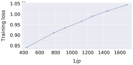
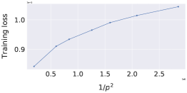
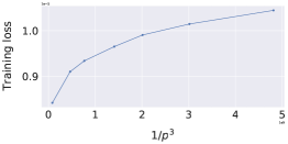
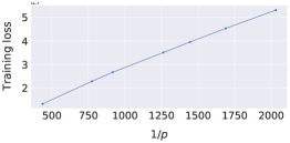
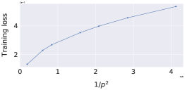
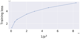
The effect of p𝑝p. First, in Figure 1 we verify the expected 𝒪(1p)𝒪1𝑝\mathcal{O}\big{(}\frac{1}{p}\big{)} dependence when c𝑐c is a constant. For a fixed n=300𝑛300n=300 number of nodes with d=100𝑑100d=100 we vary the value of a parameter p𝑝p by interpolating the ring topology (with uniform weights) with the fully-connected graph. The loss value f(𝐱())𝑓superscript𝐱f(\mathbf{x}^{(\infty)}) scales linearly in 1p1𝑝\frac{1}{p} as can be observed in Figure 1 and the dependency on p𝑝p can thus not further be improved.

Refer to caption
(a) 1/p1𝑝1/p (constant c𝑐c).
Refer to caption
(b) 1/p21superscript𝑝21/p^{2} (constant c𝑐c).
Refer to caption
(c) 1/p31superscript𝑝31/p^{3} (constant c𝑐c).
Figure 1: Impact of p𝑝p on convergence with the stochastic noise σ2=1superscript𝜎21\sigma^{2}=1, when c𝑐c and γ𝛾\gamma are kept constant. We see a linear scaling in 1p1𝑝\frac{1}{p} that verifies the 𝒪(1p)𝒪1𝑝\mathcal{O}\big{(}\frac{1}{p}\big{)}, dependence rather than prior predicted 𝒪(1p2)𝒪1superscript𝑝2\mathcal{O}\big{(}\frac{1}{p^{2}}\big{)}.

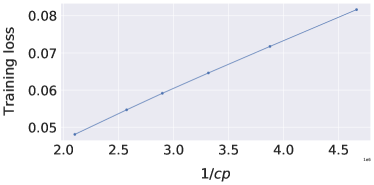
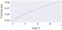
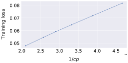
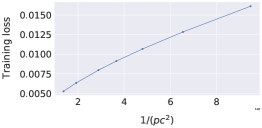
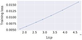
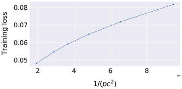
The effect of c𝑐c. In Figure 2 we aim to examine the dependence of the term 𝒪(1pc2)𝒪1𝑝superscript𝑐2\mathcal{O}\big{(}\frac{1}{pc^{2}}\big{)} on the parameter c𝑐c, in terms of 1/(pc2)1𝑝superscript𝑐21/(pc^{2}) and 1/(cp)1𝑐𝑝1/(cp). We take the ring topology on a fixed number of n=300𝑛300n=300 nodes and reduce the self-weights to achieve different values of c𝑐c (see appendix for details). Otherwise the setup is as above. The current numerical results may suggest the existence of a potentially better theoretical dependence of the term c𝑐c (as discussed in Section 4.2); we leave the study for future work.
Refer to caption
(a) 1/(pc2)1𝑝superscript𝑐21/(pc^{2}) (constant p𝑝p).
Refer to caption
(b) 1/(cp)1𝑐𝑝1/(cp) (constant p𝑝p).
Figure 2: Impact of c𝑐c on the convergence with the stochastic noise σ2=1superscript𝜎21\sigma^{2}=1, when p𝑝p and γ𝛾\gamma are kept constant. We see a near linear scaling in 𝒪(1pc)𝒪1𝑝𝑐\mathcal{O}\bigl{(}\frac{1}{pc}\big{)} while the estimate 𝒪(1pc2)𝒪1𝑝superscript𝑐2\mathcal{O}\bigl{(}\frac{1}{pc^{2}}\bigr{)} appears to be too conservative on this problem.

8 Conclusion

We have derived improved complexity bounds for the GT method, that improve over all previous results. We verify the tightness of the second term in the convergence rate in numerical experiments. Our analysis identifies that the smallest eigenvalue of the mixing matrix has a strong impact on the performance of GT, however the smallest eigenvalue can often be controlled in practice by choosing large enough self-weights (wiisubscript𝑤𝑖𝑖w_{ii}) on the nodes.

Our proof technique might be of independent interest in the community and might lead to improved analyses for other gossip based methods where the mixing matrix is not contracting (for e.g. in directed graphs, or using row- or column-stochastic matrices).

Acknowledgments and Disclosure of Funding

This project was supported by SNSF grant 200020_200342, EU project DIGIPREDICT, and a Google PhD Fellowship. The authors thank Martin Jaggi for his support.

References

  • Alghunaim et al. [2021] Sulaiman Alghunaim, Ernest Ryu, Kun Yuan, and Ali Sayed. Decentralized proximal gradient algorithms with linear convergence rates. IEEE Transactions on Automatic Control, 66(6), 2021.
  • Alghunaim and Sayed [2020] Sulaiman A. Alghunaim and Ali H. Sayed. Linear convergence of primal–dual gradient methods and their performance in distributed optimization. Automatica, 117:109003, 2020.
  • Assran et al. [2019] Mahmoud Assran, Nicolas Loizou, Nicolas Ballas, and Michael Rabbat. Stochastic gradient push for distributed deep learning. In Proceedings of the 36th International Conference on Machine Learning (ICML). PMLR, 2019.
  • Boyd et al. [2006] Stephen Boyd, Arpita Ghosh, Balaji Prabhakar, and Devavrat Shah. Randomized gossip algorithms. IEEE/ACM Trans. Netw., 14(SI):2508–2530, 2006.
  • Dekel et al. [2012] Ofer Dekel, Ran Gilad-Bachrach, Ohad Shamir, and Lin Xiao. Optimal distributed online prediction using mini-batches. Journal of Machine Learning Resesearch (JMLR), 13(1):165–202, 2012.
  • Duchi et al. [2012] J. C. Duchi, A. Agarwal, and M. J. Wainwright. Dual averaging for distributed optimization: Convergence analysis and network scaling. IEEE Transactions on Automatic Control, 57(3):592–606, 2012.
  • Gerschgorin [1931] S. Gerschgorin. Uber die Abgrenzung der Eigenwerte einer Matrix. Bulletin de l’Académie des Sciences de l’URSS. Classe des sciences mathématiques et na, 6:749–754, 1931.
  • He et al. [2018] Lie He, An Bian, and Martin Jaggi. COLA: Decentralized linear learning. In Advances in Neural Information Processing Systems 31 (NeurIPS), pages 4541–4551. Curran Associates, Inc., 2018.
  • Inc. [2021] Wolfram Research, Inc. Mathematica, Version 12.3, 2021. Champaign, IL.
  • Iutzeler et al. [2013] Franck Iutzeler, Pascal Bianchi, Philippe Ciblat, and Walid Hachem. Asynchronous distributed optimization using a randomized alternating direction method of multipliers. In Proceedings of the 52nd IEEE Conference on Decision and Control, CDC, pages 3671–3676. IEEE, 2013.
  • Johansson et al. [2010] B. Johansson, M. Rabi, and M. Johansson. A randomized incremental subgradient method for distributed optimization in networked systems. SIAM Journal on Optimization, 20(3):1157–1170, 2010.
  • Kairouz et al. [2021] Peter Kairouz, H. Brendan McMahan, Brendan Avent, Aurélien Bellet, Mehdi Bennis, Arjun Nitin Bhagoji, Keith Bonawitz, Zachary Charles, Graham Cormode, Rachel Cummings, Rafael G. L. D’Oliveira, Hubert Eichner, Salim El Rouayheb, David Evans, Josh Gardner, Zachary Garrett, Adrià Gascón, Badih Ghazi, Phillip B. Gibbons, Marco Gruteser, Zaid Harchaoui, Chaoyang He, Lie He, Zhouyuan Huo, Ben Hutchinson, Justin Hsu, Martin Jaggi, Tara Javidi, Gauri Joshi, Mikhail Khodak, Jakub Konečný, Aleksandra Korolova, Farinaz Koushanfar, Sanmi Koyejo, Tancrède Lepoint, Yang Liu, Prateek Mittal, Mehryar Mohri, Richard Nock, Ayfer Özgür, Rasmus Pagh, Mariana Raykova, Hang Qi, Daniel Ramage, Ramesh Raskar, Dawn Song, Weikang Song, Sebastian U. Stich, Ziteng Sun, Ananda Theertha Suresh, Florian Tramèr, Praneeth Vepakomma, Jianyu Wang, Li Xiong, Zheng Xu, Qiang Yang, Felix X. Yu, Han Yu, and Sen Zhao. Advances and open problems in federated learning. Foundations and Trends® in Machine Learning, 14(1–2):1–210, 2021.
  • Karimireddy et al. [2019] Sai P. Karimireddy, Satyen Kale, Mehryar Mohri, Sashank J. Reddi, Sebastian U. Stich, and Ananda T. Suresh. SCAFFOLD: Stochastic controlled averaging for on-device federated learning. In Proceedings of the 36th International Conference on Machine Learning (ICML). PMLR, 2019.
  • Kempe et al. [2003] David Kempe, Alin Dobra, and Johannes Gehrke. Gossip-based computation of aggregate information. In Proceedings of the 44th Annual IEEE Symposium on Foundations of Computer Science (FOCS). IEEE Computer Society, 2003.
  • Koloskova et al. [2019] Anastasia Koloskova, Sebastian Stich, and Martin Jaggi. Decentralized stochastic optimization and gossip algorithms with compressed communication. In Proceedings of the 36th International Conference on Machine Learning (ICML), volume 97, pages 3478–3487. PMLR, 2019.
  • Koloskova et al. [2020] Anastasia Koloskova, Nicolas Loizou, Sadra Boreiri, Martin Jaggi, and Sebastian U. Stich. A unified theory of decentralized sgd with changing topology and local updates. In Proceedings of the 37th International Conference on Machine Learning (ICML). PMLR, 2020.
  • Konečnỳ et al. [2016] Jakub Konečnỳ, H. Brendan McMahan, Daniel Ramage, and Peter Richtárik. Federated optimization: Distributed machine learning for on-device intelligence. arXiv preprint arXiv:1610.02527, 2016.
  • Kong et al. [2021] Lingjing Kong, Tao Lin, Anastasia Koloskova, Martin Jaggi, and Sebastian U. Stich. Consensus control for decentralized deep learning. In Proceedings of the 38th International Conference on Machine Learning (ICML), volume 139, pages 5686–5696. PMLR, 2021.
  • Kovalev et al. [2021] Dmitry Kovalev, Anastasia Koloskova, Martin Jaggi, Peter Richtarik, and Sebastian U. Stich. A linearly convergent algorithm for decentralized optimization: Sending less bits for free! In Proceedings of The 24th International Conference on Artificial Intelligence and Statistics (AISTATS), volume 130, pages 4087–4095. PMLR, 2021.
  • Li et al. [2020a] Boyue Li, Shicong Cen, Yuxin Chen, and Yuejie Chi. Communication-efficient distributed optimization in networks with gradient tracking and variance reduction. In Proceedings of the Twenty Third International Conference on Artificial Intelligence and Statistics (AISTATS), volume 108, pages 1662–1672. PMLR, 2020a.
  • Li et al. [2018] Tian Li, Anit Kumar Sahu, Maziar Sanjabi, Manzil Zaheer, Ameet Talwalkar, and Virginia Smith. On the convergence of federated optimization in heterogeneous networks. arXiv preprint arXiv:1812.06127, 2018.
  • Li et al. [2020b] Tian Li, Anit Kumar Sahu, Manzil Zaheer, Maziar Sanjabi, Ameet Talwalkar, and Virginia Smith. FedDANE: A federated Newton-type method. arXiv preprint arXiv:2001.01920, 2020b.
  • Li et al. [2020c] Xiang Li, Kaixuan Huang, Wenhao Yang, Shusen Wang, and Zhihua Zhang. On the convergence of FedAvg on non-IID data. International Conference on Learning Representations (ICLR), 2020c.
  • Lian et al. [2017] Xiangru Lian, Ce Zhang, Huan Zhang, Cho-Jui Hsieh, Wei Zhang, and Ji Liu. Can decentralized algorithms outperform centralized algorithms? a case study for decentralized parallel stochastic gradient descent. In Advances in Neural Information Processing Systems 30 (NIPS), pages 5330–5340. Curran Associates, Inc., 2017.
  • Lin et al. [2021] Tao Lin, Sai Praneeth Karimireddy, Sebastian Stich, and Martin Jaggi. Quasi-global momentum: Accelerating decentralized deep learning on heterogeneous data. In Proceedings of the 38th International Conference on Machine Learning (ICML), volume 139, pages 6654–6665. PMLR, 2021.
  • Lorenzo and Scutari [2016] Paolo Di Lorenzo and Gesualdo Scutari. NEXT: In-network nonconvex optimization. IEEE Transactions on Signal and Information Processing over Networks, 2(2):120–136, 2016.
  • Lu et al. [2019] Songtao Lu, Xinwei Zhang, Haoran Sun, and Mingyi Hong. GNSD: a gradient-tracking based nonconvex stochastic algorithm for decentralized optimization. In IEEE Data Science Workshop (DSW), pages 315–321, 2019.
  • McMahan et al. [2017] Brendan McMahan, Eider Moore, Daniel Ramage, Seth Hampson, and Blaise Agüera y Arcas. Communication-efficient learning of deep networks from decentralized data. In Proceedings of the 20th International Conference on Artificial Intelligence and Statistics (AISTATS), pages 1273–1282, 2017.
  • McMahan et al. [2016] H. Brendan McMahan, Eider Moore, Daniel Ramage, and Blaise Agüera y Arcas. Federated learning of deep networks using model averaging. arXiv preprint arXiv:1602.05629, 2016.
  • Nedić and Ozdaglar [2009] A. Nedić and A. Ozdaglar. Distributed subgradient methods for multi-agent optimization. IEEE Transactions on Automatic Control, 54(1):48–61, 2009.
  • Nedić et al. [2015] A. Nedić, S. Lee, and M. Raginsky. Decentralized online optimization with global objectives and local communication. In 2015 American Control Conference (ACC), pages 4497–4503, 2015.
  • Nedić and Olshevsky [2014] Angelia Nedić and Alex Olshevsky. Distributed optimization over time-varying directed graphs. IEEE Transactions on Automatic Control, 60(3):601–615, 2014.
  • Nedić [2020] Angelia Nedić. Distributed gradient methods for convex machine learning problems in networks: Distributed optimization. IEEE Signal Processing Magazine, 37(3):92–101, 2020.
  • Nedić et al. [2016] Angelia Nedić, Alex Olshevsky, and Wei Shi. Achieving geometric convergence for distributed optimization over time-varying graphs. SIAM Journal on Optimization, 27, 07 2016.
  • Nedić et al. [2017] Angelia Nedić, Alex Olshevsky, Wei Shi, and César A. Uribe. Geometrically convergent distributed optimization with uncoordinated step-sizes. In 2017 American Control Conference (ACC), pages 3950–3955, 2017.
  • Nedić et al. [2018] Angelia Nedić, Alex Olshevsky, and Michael G. Rabbat. Network topology and communication-computation tradeoffs in decentralized optimization. Proceedings of the IEEE, 106(5):953–976, 2018.
  • Nemirovsky and Yudin [1983] Arkadii Semenovich Nemirovsky and David Borisovich Yudin. Problem complexity and method efficiency in optimization. Wiley, 1983.
  • Nguyen et al. [2019] Lam M. Nguyen, Phuong Ha Nguyen, Peter Richtárik, Katya Scheinberg, Martin Takáč, and Marten van Dijk. New convergence aspects of stochastic gradient algorithms. Journal of Machine Learning Research, 20(176):1–49, 2019.
  • Pu and Nedić [2020] Shi Pu and Angelia Nedić. Distributed stochastic gradient tracking methods. Math. Program., 187:409–457, 2020.
  • Qu and Li [2017] Guannan Qu and Na Li. Harnessing smoothness to accelerate distributed optimization. IEEE Transactions on Control of Network Systems, 2017.
  • Rabbat [2015] M. Rabbat. Multi-agent mirror descent for decentralized stochastic optimization. In IEEE 6th International Workshop on Computational Advances in Multi-Sensor Adaptive Processing (CAMSAP), pages 517–520, 2015.
  • Shi et al. [2015] Wei Shi, Qing Ling, Gang Wu, and Wotao Yin. EXTRA: An exact first-order algorithm for decentralized consensus optimization. SIAM Journal on Optimization, 25(2):944–966, 2015.
  • Stich [2019] Sebastian U. Stich. Unified optimal analysis of the (stochastic) gradient method. arXiv preprint arXiv:1907.04232, 2019.
  • Stich and Karimireddy [2020] Sebastian U. Stich and Sai P. Karimireddy. The error-feedback framework: Better rates for SGD with delayed gradients and compressed communication. Journal of Machine Learning Research, 21(237):1–36, 2020.
  • Tang et al. [2018a] Hanlin Tang, Shaoduo Gan, Ce Zhang, Tong Zhang, and Ji Liu. Communication compression for decentralized training. In Advances in Neural Information Processing Systems 31 (NeurIPS), pages 7663–7673. Curran Associates, Inc., 2018a.
  • Tang et al. [2018b] Hanlin Tang, Xiangru Lian, Ming Yan, Ce Zhang, and Ji Liu. D2: Decentralized training over decentralized data. In Proceedings of the 35th International Conference on Machine Learning (ICML), volume 80, pages 4848–4856. PMLR, 2018b.
  • Tang et al. [2019] Hanlin Tang, Xiangru Lian, Shuang Qiu, Lei Yuan, Ce Zhang, Tong Zhang, and Ji Liu. Deepsqueeze: Decentralization meets error-compensated compression. arXiv preprint arXiv:1907.07346, 2019.
  • Tsitsiklis [1984] John N. Tsitsiklis. Problems in decentralized decision making and computation. PhD thesis, Massachusetts Institute of Technology, 1984.
  • Tziotis et al. [2020] Isidoros Tziotis, Constantine Caramanis, and Aryan Mokhtari. Second order optimality in decentralized non-convex optimization via perturbed gradient tracking. In Advances in Neural Information Processing Systems (NeurIPS), volume 33, pages 21162–21173. Curran Associates, Inc., 2020.
  • Vogels et al. [2021] Thijs Vogels, Lie He, Anastasia Koloskova, Tao Lin, Sai Praneeth Karimireddy, Sebastian U. Stich, and Martin Jaggi. Relaysum for decentralized deep learning on heterogeneous data. In Advances in Neural Information Processing Systems (NeurIPS). Curran Associates, Inc., 2021.
  • Wang et al. [2019] Jianyu Wang, Anit Kumar Sahu, Zhouyi Yang, Gauri Joshi, and Soummya Kar. MATCHA: Speeding up decentralized SGD via matching decomposition sampling. In 2019 Sixth Indian Control Conference (ICC), pages 299–300, 2019.
  • Wei and Ozdaglar [2012] E. Wei and A. Ozdaglar. Distributed alternating direction method of multipliers. In IEEE 51st IEEE Conference on Decision and Control (CDC), pages 5445–5450, 2012.
  • Xiao and Boyd [2004] Lin Xiao and Stephen Boyd. Fast linear iterations for distributed averaging. Systems & Control Letters, 53(1):65–78, 2004.
  • Xin et al. [2019] Ran Xin, Anit Kumar Sahu, Usman A. Khan, and Soummya Kar. Distributed stochastic optimization with gradient tracking over strongly-connected networks. In IEEE 58th Conference on Decision and Control (CDC), pages 8353–8358, 2019.
  • Yuan and Alghunaim [2021] Kun Yuan and Sulaiman A. Alghunaim. Removing data heterogeneity influence enhances network topology dependence of decentralized SGD. arXiv preprint arXiv:2105.08023, 2021.
  • Yuan et al. [2019a] Kun Yuan, Bicheng Ying, Xiaochuan Zhao, and Ali H. Sayed. Exact diffusion for distributed optimization and learning - part I: algorithm development. IEEE Trans. Signal Process., 67(3):708–723, 2019a.
  • Yuan et al. [2019b] Kun Yuan, Bicheng Ying, Xiaochuan Zhao, and Ali H. Sayed. Exact diffusion for distributed optimization and learning - part II: convergence analysis. IEEE Trans. Signal Process., 67(3):724–739, 2019b.
  • Yuan et al. [2020] Kun Yuan, Wei Xu, and Qing Ling. Can primal methods outperform primal-dual methods in decentralized dynamic optimization? IEEE Transactions on Signal Processing, 68:4466–4480, 2020.
  • Yuan et al. [2021] Kun Yuan, Yiming Chen, Xinmeng Huang, Yingya Zhang, Pan Pan, Yinghui Xu, and Wotao Yin. DecentLaM: Decentralized momentum SGD for large-batch deep training. In Proceedings of the IEEE/CVF International Conference on Computer Vision (ICCV), pages 3029–3039, 2021.
  • Zhang and You [2020] Jiaqi Zhang and Keyou You. Decentralized stochastic gradient tracking for non-convex empirical risk minimization. arXiv preprint arXiv:1909.02712, 2020.
  • Zhu and Martínez [2010] Minghui Zhu and Sonia Martínez. Discrete-time dynamic average consensus. Automatica, 46(2):322–329, 2010. ISSN 0005-1098.

Appendix A Proof of Theorem 3 — Consensus Functions

We consider functions fi(𝐱)=12𝐱𝝁i2subscript𝑓𝑖𝐱12superscriptdelimited-∥∥𝐱subscript𝝁𝑖2f_{i}(\mathbf{x})=\frac{1}{2}\left\lVert\mathbf{x}-\bm{\mu}_{i}\right\rVert^{2}, where 𝐱,𝝁id𝐱subscript𝝁𝑖superscript𝑑\mathbf{x},\bm{\mu}_{i}\in\mathbb{R}^{d}. Then fi(𝐱)=𝐱𝝁isubscript𝑓𝑖𝐱𝐱subscript𝝁𝑖\nabla f_{i}(\mathbf{x})=\mathbf{x}-\bm{\mu}_{i}. In matrix notation, the GT algorithm in this special case is equivalent to

(X(t+1)γY(t+1))=(X(t)γY(t))(WW0W)+γ(0X(t+1)X(t))=(X(t)γY(t))(WWγ(WI)(1γ)W).superscriptmatrixsuperscript𝑋𝑡1𝛾superscript𝑌𝑡1topsuperscriptmatrixsuperscript𝑋𝑡𝛾superscript𝑌𝑡topmatrix𝑊𝑊0𝑊𝛾superscriptmatrix0superscript𝑋𝑡1superscript𝑋𝑡topsuperscriptmatrixsuperscript𝑋𝑡𝛾superscript𝑌𝑡topmatrix𝑊𝑊𝛾𝑊𝐼1𝛾𝑊\displaystyle\begin{pmatrix}X^{(t+1)}\\ \gamma Y^{(t+1)}\end{pmatrix}^{\top}=\begin{pmatrix}X^{(t)}\\ \gamma Y^{(t)}\end{pmatrix}^{\top}\begin{pmatrix}W&-W\\ 0&W\end{pmatrix}+\gamma\begin{pmatrix}0\\ X^{(t+1)}-X^{(t)}\end{pmatrix}^{\top}=\begin{pmatrix}X^{(t)}\\ \gamma Y^{(t)}\end{pmatrix}^{\top}\begin{pmatrix}W&-W\\ \gamma(W-I)&(1-\gamma)W\end{pmatrix}\,.

The optimal point 𝐱=𝝁¯=1ni=1n𝝁𝒊superscript𝐱bold-¯𝝁1𝑛superscriptsubscript𝑖1𝑛subscript𝝁𝒊\mathbf{x}^{\star}=\bm{\bar{\mu}}=\frac{1}{n}\sum_{i=1}^{n}\bm{\mu_{i}}. Denote X=[𝐱,,𝐱]d×nsuperscript𝑋superscript𝐱superscript𝐱superscript𝑑𝑛X^{\star}=\left[\mathbf{x}^{\star},\dots,\mathbf{x}^{\star}\right]\in\mathbb{R}^{d\times n}. We decompose the error as

X(t)XF2=X(t)X¯(t)F2consensus error+X¯(t)X2optimization error.superscriptsubscriptdelimited-∥∥superscript𝑋𝑡superscript𝑋𝐹2subscriptsuperscriptsubscriptdelimited-∥∥superscript𝑋𝑡superscript¯𝑋𝑡𝐹2consensus errorsubscriptsuperscriptdelimited-∥∥superscript¯𝑋𝑡superscript𝑋2optimization error\displaystyle\left\lVert X^{(t)}-X^{\star}\right\rVert_{F}^{2}=\underbrace{\left\lVert X^{(t)}-\bar{X}^{(t)}\right\rVert_{F}^{2}}_{\text{consensus error}}+\underbrace{\left\lVert\bar{X}^{(t)}-X^{\star}\right\rVert^{2}}_{\text{optimization error}}\,.
For the optimization part,

notice that Y¯(t)=X¯(t)Xsuperscript¯𝑌𝑡superscript¯𝑋𝑡superscript𝑋\bar{Y}^{(t)}=\bar{X}^{(t)}-X^{\star}. That is because

Y¯(0)=f(X(0))1n𝟏𝟏=X¯(0)X,superscript¯𝑌0𝑓superscript𝑋01𝑛superscript11topsuperscript¯𝑋0superscript𝑋\displaystyle\bar{Y}^{(0)}=\nabla f(X^{(0)})\frac{1}{n}\mathbf{1}\mathbf{1}^{\top}=\bar{X}^{(0)}-X^{\star}, Y¯(t+1)=Y¯(t)+X¯(t+1)X¯(t).superscript¯𝑌𝑡1superscript¯𝑌𝑡superscript¯𝑋𝑡1superscript¯𝑋𝑡\displaystyle\bar{Y}^{(t+1)}=\bar{Y}^{(t)}+\bar{X}^{(t+1)}-\bar{X}^{(t)}\,.

Therefore, the optimization error is equal to

X¯tXF2superscriptsubscriptdelimited-∥∥superscript¯𝑋𝑡superscript𝑋𝐹2\displaystyle\left\lVert\bar{X}^{t}-X^{\star}\right\rVert_{F}^{2} =X¯(t1)γY¯(t1)XF2=(1γ)(X¯(t1)X)F2absentsuperscriptsubscriptdelimited-∥∥superscript¯𝑋𝑡1𝛾superscript¯𝑌𝑡1superscript𝑋𝐹2superscriptsubscriptdelimited-∥∥1𝛾superscript¯𝑋𝑡1superscript𝑋𝐹2\displaystyle=\left\lVert\bar{X}^{(t-1)}-\gamma\bar{Y}^{(t-1)}-X^{\star}\right\rVert_{F}^{2}=\left\lVert(1-\gamma)\left(\bar{X}^{(t-1)}-X^{\star}\right)\right\rVert_{F}^{2}
=(1γ)2tX¯(0)XF2.absentsuperscript1𝛾2𝑡superscriptsubscriptdelimited-∥∥superscript¯𝑋0superscript𝑋𝐹2\displaystyle=(1-\gamma)^{2t}\left\lVert\bar{X}^{(0)}-X^{\star}\right\rVert_{F}^{2}\,.
For the consensus part,

denoting, W~=W𝟏𝟏n~𝑊𝑊superscript11top𝑛\tilde{W}=W-\frac{\mathbf{1}\mathbf{1}^{\top}}{n}, ΔX(t)=X(t)X¯(t)Δsuperscript𝑋𝑡superscript𝑋𝑡superscript¯𝑋𝑡\Delta X^{(t)}=X^{(t)}-\bar{X}^{(t)}, ΔY(t)=Y(t)Y¯(t)Δsuperscript𝑌𝑡superscript𝑌𝑡superscript¯𝑌𝑡\Delta Y^{(t)}=Y^{(t)}-\bar{Y}^{(t)},

(ΔX(t)γΔY(t))=(ΔX(0)γΔY(0))(W~W~γ(WI)(1γ)W~)tJ.superscriptmatrixΔsuperscript𝑋𝑡𝛾Δsuperscript𝑌𝑡topsuperscriptmatrixΔsuperscript𝑋0𝛾Δsuperscript𝑌0topsubscriptsuperscriptmatrix~𝑊~𝑊𝛾𝑊𝐼1𝛾~𝑊𝑡superscript𝐽\displaystyle\begin{pmatrix}\Delta X^{(t)}\\ \gamma\Delta Y^{(t)}\end{pmatrix}^{\top}=\begin{pmatrix}\Delta X^{(0)}\\ \gamma\Delta Y^{(0)}\end{pmatrix}^{\top}\underbrace{\begin{pmatrix}\tilde{W}&-\tilde{W}\\ \gamma(W-I)&(1-\gamma)\tilde{W}\end{pmatrix}^{t}}_{J^{\prime}}\,.

Taking the norm,

ΔX(t)F2+γ2ΔY(t)F2Jt22(ΔX(0)F2+γ2ΔY(0)F2).superscriptsubscriptdelimited-∥∥Δsuperscript𝑋𝑡𝐹2superscript𝛾2superscriptsubscriptdelimited-∥∥Δsuperscript𝑌𝑡𝐹2superscriptsubscriptdelimited-∥∥superscript𝐽𝑡22superscriptsubscriptdelimited-∥∥Δsuperscript𝑋0𝐹2superscript𝛾2superscriptsubscriptdelimited-∥∥Δsuperscript𝑌0𝐹2\displaystyle\left\lVert\Delta X^{(t)}\right\rVert_{F}^{2}+\gamma^{2}\left\lVert\Delta Y^{(t)}\right\rVert_{F}^{2}\leq\left\lVert J^{\prime t}\right\rVert_{2}^{2}\left(\left\lVert\Delta X^{(0)}\right\rVert_{F}^{2}+\gamma^{2}\left\lVert\Delta Y^{(0)}\right\rVert_{F}^{2}\right)\,.

Lets analyze spectral properties of matrix Jtsuperscript𝐽𝑡J^{\prime t}. Let the eigenvalue decomposition of W𝑊W be W=UΛU𝑊𝑈Λsuperscript𝑈topW=U\Lambda U^{\top}, the eigenvalue decomposition of W~~𝑊\tilde{W} is W~=UΛ~U~𝑊𝑈~Λsuperscript𝑈top\tilde{W}=U\tilde{\Lambda}U^{\top} for diagonal Λ~~Λ\tilde{\Lambda}.

We can decompose

J=(U00U)(Λ~Λ~γ(ΛI)(1γ)Λ~)=:M(U00U).superscript𝐽matrix𝑈00𝑈subscriptmatrix~Λ~Λ𝛾Λ𝐼1𝛾~Λ:absent𝑀matrixsuperscript𝑈top00superscript𝑈top\displaystyle J^{\prime}=\begin{pmatrix}U&0\\ 0&U\end{pmatrix}\underbrace{\begin{pmatrix}\tilde{\Lambda}&-\tilde{\Lambda}\\ \gamma\left(\Lambda-I\right)&(1-\gamma)\tilde{\Lambda}\end{pmatrix}}_{=:M}\begin{pmatrix}U^{\top}&0\\ 0&U^{\top}\end{pmatrix}\,.

And,

Jt22=(U00U)(Λ~Λ~γ(ΛI)(1γ)Λ~)t(U00U)22=(Λ~Λ~γ(ΛI)(1γ)Λ~)t22,superscriptsubscriptdelimited-∥∥superscript𝐽𝑡22superscriptsubscriptdelimited-∥∥matrix𝑈00𝑈superscriptmatrix~Λ~Λ𝛾Λ𝐼1𝛾~Λ𝑡matrixsuperscript𝑈top00superscript𝑈top22superscriptsubscriptdelimited-∥∥superscriptmatrix~Λ~Λ𝛾Λ𝐼1𝛾~Λ𝑡22\displaystyle\left\lVert J^{\prime t}\right\rVert_{2}^{2}=\left\lVert\begin{pmatrix}U&0\\ 0&U\end{pmatrix}\begin{pmatrix}\tilde{\Lambda}&-\tilde{\Lambda}\\ \gamma\left(\Lambda-I\right)&(1-\gamma)\tilde{\Lambda}\end{pmatrix}^{t}\begin{pmatrix}U^{\top}&0\\ 0&U^{\top}\end{pmatrix}\right\rVert_{2}^{2}=\left\lVert\begin{pmatrix}\tilde{\Lambda}&-\tilde{\Lambda}\\ \gamma\left(\Lambda-I\right)&(1-\gamma)\tilde{\Lambda}\end{pmatrix}^{t}\right\rVert_{2}^{2},

where the last equality is due to unitary property of U𝑈U.

Lemma 9.

To diagonalize a block-diagonal matrix

(ABCD),matrix𝐴𝐵𝐶𝐷\displaystyle\begin{pmatrix}A&B\\ C&D\end{pmatrix},

where A=diag(a0,an)Rn×n𝐴diagsubscript𝑎0subscript𝑎𝑛superscript𝑅𝑛𝑛A=\operatorname*{diag}(a_{0},\dots a_{n})\in R^{n\times n}, B=diag(b0,,bn)𝐵diagsubscript𝑏0subscript𝑏𝑛B=\operatorname*{diag}(b_{0},\dots,b_{n}), C=diag(c0,,cn)𝐶diagsubscript𝑐0subscript𝑐𝑛C=\operatorname*{diag}(c_{0},\dots,c_{n}), D=diag(d0,,dn)𝐷diagsubscript𝑑0subscript𝑑𝑛D=\operatorname*{diag}(d_{0},\dots,d_{n}). Assume that each of the 2×2222\times 2 matrices

(aibicidi)matrixsubscript𝑎𝑖subscript𝑏𝑖subscript𝑐𝑖subscript𝑑𝑖\displaystyle\begin{pmatrix}a_{i}&b_{i}\\ c_{i}&d_{i}\end{pmatrix}

are diagonalizable with

(aibicidi)=(qi(1)qi(2)qi(3)qi(4))(di(1)00di(2))(qi(1)qi(2)qi(3)qi(4))matrixsubscript𝑎𝑖subscript𝑏𝑖subscript𝑐𝑖subscript𝑑𝑖matrixsubscriptsuperscript𝑞1𝑖subscriptsuperscript𝑞2𝑖subscriptsuperscript𝑞3𝑖subscriptsuperscript𝑞4𝑖matrixsubscriptsuperscript𝑑1𝑖00subscriptsuperscript𝑑2𝑖matrixsubscriptsuperscript𝑞1𝑖subscriptsuperscript𝑞2𝑖subscriptsuperscript𝑞3𝑖subscriptsuperscript𝑞4𝑖\displaystyle\begin{pmatrix}a_{i}&b_{i}\\ c_{i}&d_{i}\end{pmatrix}=\begin{pmatrix}q^{(1)}_{i}&q^{(2)}_{i}\\ q^{(3)}_{i}&q^{(4)}_{i}\end{pmatrix}\cdot\begin{pmatrix}d^{(1)}_{i}&0\\ 0&d^{(2)}_{i}\end{pmatrix}\cdot\begin{pmatrix}q^{(-1)}_{i}&q^{(-2)}_{i}\\ q^{(-3)}_{i}&q^{(-4)}_{i}\end{pmatrix}

Then the original matrix is diagonalizable and its diagonalization is equal to

(ABCD)=(Q1Q2Q3Q4)(D100D2)(Q1Q2Q3Q4),matrix𝐴𝐵𝐶𝐷matrixsubscript𝑄1subscript𝑄2subscript𝑄3subscript𝑄4matrixsubscript𝐷100subscript𝐷2matrixsubscript𝑄1subscript𝑄2subscript𝑄3subscript𝑄4\displaystyle\begin{pmatrix}A&B\\ C&D\end{pmatrix}=\begin{pmatrix}Q_{1}&Q_{2}\\ Q_{3}&Q_{4}\end{pmatrix}\cdot\begin{pmatrix}D_{1}&0\\ 0&D_{2}\end{pmatrix}\cdot\begin{pmatrix}Q_{-1}&Q_{-2}\\ Q_{-3}&Q_{-4}\end{pmatrix},

where each Ql=diag(q1(l),,qn(l))subscript𝑄𝑙diagsuperscriptsubscript𝑞1𝑙superscriptsubscript𝑞𝑛𝑙Q_{l}=\operatorname*{diag}\left(q_{1}^{(l)},\dots,q_{n}^{(l)}\right), Dl=diag(d1(l),dn(l))subscript𝐷𝑙diagsuperscriptsubscript𝑑1𝑙superscriptsubscript𝑑𝑛𝑙D_{l}=\operatorname*{diag}\left(d_{1}^{(l)},\dots d_{n}^{(l)}\right).

We need to show that the following 2×2222\times 2 matrices are diagonalizable.

Mi:=(λiλiγ(λi1)(1γ)λi),assignsubscript𝑀𝑖matrixsubscript𝜆𝑖subscript𝜆𝑖𝛾subscript𝜆𝑖11𝛾subscript𝜆𝑖\displaystyle M_{i}:=\begin{pmatrix}\lambda_{i}&-\lambda_{i}\\ \gamma\left(\lambda_{i}-1\right)&(1-\gamma)\lambda_{i}\end{pmatrix},

where the λisubscript𝜆𝑖\lambda_{i} are eigenvalues of the matrix W~~𝑊\tilde{W}. The eigenvalues of Misubscript𝑀𝑖M_{i} are

λ(Mi)={λiγλi212γλi4+(γ4)λi,λiγλi2+12γλi4+(γ4)λi},𝜆subscript𝑀𝑖subscript𝜆𝑖𝛾subscript𝜆𝑖212𝛾subscript𝜆𝑖4𝛾4subscript𝜆𝑖subscript𝜆𝑖𝛾subscript𝜆𝑖212𝛾subscript𝜆𝑖4𝛾4subscript𝜆𝑖\displaystyle\lambda(M_{i})=\left\{\lambda_{i}-\frac{\gamma\lambda_{i}}{2}-\frac{1}{2}\sqrt{\gamma\lambda_{i}}\sqrt{4+(\gamma-4)\lambda_{i}},\lambda_{i}-\frac{\gamma\lambda_{i}}{2}+\frac{1}{2}\sqrt{\gamma\lambda_{i}}\sqrt{4+(\gamma-4)\lambda_{i}}\right\}\,,

which are distinct for γ>0𝛾0\gamma>0, therefore the matrix is diagonalizble (over \mathbb{C}).

If λisubscript𝜆𝑖\lambda_{i} is positive, then by choosing γ1λi𝛾1subscript𝜆𝑖\gamma\leq 1-\lambda_{i},

|λ(Mi)|13λi+23.𝜆subscript𝑀𝑖13subscript𝜆𝑖23\displaystyle\left\lvert\lambda(M_{i})\right\rvert\leq\frac{1}{3}\lambda_{i}+\frac{2}{3}\,.

If λisubscript𝜆𝑖\lambda_{i} is negative, then, then by choosing γ1|λi|𝛾1subscript𝜆𝑖\gamma\leq 1-\left\lvert\lambda_{i}\right\rvert,

|λ(Mi)|13|λi|+23.𝜆subscript𝑀𝑖13subscript𝜆𝑖23\displaystyle\left\lvert\lambda(M_{i})\right\rvert\leq\frac{1}{3}\left\lvert\lambda_{i}\right\rvert+\frac{2}{3}\,.

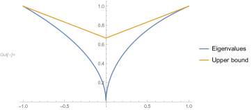
We do not give the full formal prove of these two bounds. First we note that |(Mi)|subscript𝑀𝑖\left\lvert(M_{i})\right\rvert is monotone in γ𝛾\gamma, i.e. the absolute value increases in γ𝛾\gamma. Therefore it is enough to check that it holds |λ(Mi)|13|λi|+23𝜆subscript𝑀𝑖13subscript𝜆𝑖23\left\lvert\lambda(M_{i})\right\rvert\leq\frac{1}{3}\left\lvert\lambda_{i}\right\rvert+\frac{2}{3} for γ=1|λi|𝛾1subscript𝜆𝑖\gamma=1-\left\lvert\lambda_{i}\right\rvert. We visualize these upper bounds with Mathematica [9] in Figure 3.
Refer to caption
Figure 3: The upper bound 13|λi|+2313subscript𝜆𝑖23\frac{1}{3}\left\lvert\lambda_{i}\right\rvert+\frac{2}{3} (yellow) vs. the true |λ(Mi)|𝜆subscript𝑀𝑖\left\lvert\lambda(M_{i})\right\rvert for the choice γ=1|λi|𝛾1subscript𝜆𝑖\gamma=1-\left\lvert\lambda_{i}\right\rvert.

This concludes the proof.

Appendix B Proof of Theorem 2 — General Case

We first re-state theorem 2 in terms of number of iterations T𝑇T

Theorem 10.

For GT algorithm 1 with a mixing matrix as in Definition 1, under Assumptions 1, 2, 4, after T𝑇T iterations, if T>2plog(50p(1+log1p))𝑇2𝑝50𝑝11𝑝T>\frac{2}{p}\log\left(\frac{50}{p}(1+\log\frac{1}{p})\right), there exists a constant stepsize γt=γsubscript𝛾𝑡𝛾\gamma_{t}=\gamma such that the error is bounded as
Non-convex:

1T+1t=0Tf(𝐱¯(t))22𝒪~(LF0σ2nT+(σLF0(pc+pn)T)2/3+L(F0+LR~02)pcT),1𝑇1superscriptsubscript𝑡0𝑇superscriptsubscriptdelimited-∥∥𝑓superscript¯𝐱𝑡22~𝒪𝐿subscript𝐹0superscript𝜎2𝑛𝑇superscript𝜎𝐿subscript𝐹0𝑝𝑐𝑝𝑛𝑇23𝐿subscript𝐹0𝐿superscriptsubscript~𝑅02𝑝𝑐𝑇\displaystyle\frac{1}{T+1}\sum_{t=0}^{T}\left\lVert\nabla f(\bar{\mathbf{x}}^{(t)})\right\rVert_{2}^{2}\leq\tilde{\mathcal{O}}\left(\sqrt{\frac{LF_{0}\sigma^{2}}{nT}}+\left(\frac{\sigma LF_{0}}{(\sqrt{p}c+p\sqrt{n})T}\right)^{\nicefrac{{2}}{{3}}}+\frac{L(F_{0}+L\tilde{R}_{0}^{2})}{pcT}\right)\,,

Strongly-convex: Under additional Assumption 3 with μ>0μ0\mu>0, it holds

t=0TwtWT[𝔼f(𝐱¯(t))f]+μ2RT+1𝒪~(σ2μnT+Lσ2μ2pc2T2+L(R02+LμR~02)pcexp[μpcTL]),superscriptsubscript𝑡0𝑇subscript𝑤𝑡subscript𝑊𝑇delimited-[]𝔼𝑓superscript¯𝐱𝑡superscript𝑓𝜇2subscript𝑅𝑇1~𝒪superscript𝜎2𝜇𝑛𝑇𝐿superscript𝜎2superscript𝜇2𝑝superscript𝑐2superscript𝑇2𝐿superscriptsubscript𝑅02𝐿𝜇superscriptsubscript~𝑅02𝑝𝑐𝜇𝑝𝑐𝑇𝐿\displaystyle\sum_{t=0}^{T}\frac{w_{t}}{W_{T}}\left[\operatorname{{\mathbb{E}}}f(\bar{\mathbf{x}}^{(t)})-f^{\star}\right]+\frac{\mu}{2}R_{T+1}\leq\tilde{\mathcal{O}}\left(\frac{\sigma^{2}}{\mu nT}+\frac{L\sigma^{2}}{\mu^{2}pc^{2}T^{2}}+\frac{L(R_{0}^{2}+\frac{L}{\mu}\tilde{R}_{0}^{2})}{pc}\exp\left[-\frac{\mu pcT}{L}\right]\right)\,,

Weakly-convex: Under Assumptions 3 with μ0μ0\mu\geq 0, it holds

1T+1t=0T[𝔼f(𝐱¯(t))f]𝒪~(R02σ2nT+(σLR02pcT)2/3+L(R02+R~02)pcT),1𝑇1superscriptsubscript𝑡0𝑇delimited-[]𝔼𝑓superscript¯𝐱𝑡superscript𝑓~𝒪superscriptsubscript𝑅02superscript𝜎2𝑛𝑇superscript𝜎𝐿superscriptsubscript𝑅02𝑝𝑐𝑇23𝐿superscriptsubscript𝑅02superscriptsubscript~𝑅02𝑝𝑐𝑇\displaystyle\frac{1}{T+1}\sum_{t=0}^{T}\left[\operatorname{{\mathbb{E}}}f(\bar{\mathbf{x}}^{(t)})-f^{\star}\right]\leq\tilde{\mathcal{O}}\left(\sqrt{\frac{R_{0}^{2}\sigma^{2}}{nT}}+\left(\frac{\sigma\sqrt{L}R_{0}^{2}}{\sqrt{p}cT}\right)^{\nicefrac{{2}}{{3}}}+\frac{L(R_{0}^{2}+\tilde{R}_{0}^{2})}{pcT}\right)\,,

where F0=f(𝐱¯(0))fsubscript𝐹0𝑓superscript¯𝐱0superscript𝑓F_{0}=f(\bar{\mathbf{x}}^{(0)})-f^{\star}, Rt=𝐱(t)𝐱subscript𝑅𝑡delimited-∥∥superscript𝐱𝑡superscript𝐱R_{t}=\left\lVert\mathbf{x}^{(t)}-\mathbf{x}^{\star}\right\rVert, t{0,T+1}𝑡0𝑇1t\in\{0,T+1\}, R~02=1ni=1n𝐱i(0)𝐱¯(0)2+1ni=1n𝐲i(0)𝐲¯(0)2superscriptsubscript~𝑅021𝑛superscriptsubscript𝑖1𝑛superscriptdelimited-∥∥superscriptsubscript𝐱𝑖0superscript¯𝐱021𝑛superscriptsubscript𝑖1𝑛superscriptdelimited-∥∥superscriptsubscript𝐲𝑖0superscript¯𝐲02\tilde{R}_{0}^{2}=\frac{1}{n}\sum_{i=1}^{n}\left\lVert\mathbf{x}_{i}^{(0)}-\bar{\mathbf{x}}^{(0)}\right\rVert^{2}+\frac{1}{n}\sum_{i=1}^{n}\left\lVert\mathbf{y}_{i}^{(0)}-\bar{\mathbf{y}}^{(0)}\right\rVert^{2}.

B.1 Useful Inequalities

Proof of Lemma 4.

By monotonicity, it suffices to check the inequality for i=τ𝑖𝜏i=\tau. By using (1p)ieipsuperscript1𝑝𝑖superscript𝑒𝑖𝑝(1-p)^{i}\leq e^{-ip} and plugging τ𝜏\tau into (10) it follows:

Ji2superscriptdelimited-∥∥superscript𝐽𝑖2\displaystyle\left\lVert J^{i}\right\rVert^{2} eτp(1+τ2)p2502(1+log1p)2(1+(2(log(50)+log(1p(1+log1p)))2p2)\displaystyle\leq e^{-\tau p}(1+\tau^{2})\leq\frac{p^{2}}{50^{2}(1+\log\frac{1}{p})^{2}}\left(1+\frac{(2(\log(50)+\log(\frac{1}{p}(1+\log\frac{1}{p})))^{2}}{p^{2}}\right)
1502+110+14absent1superscript50211014\displaystyle\leq\frac{1}{50^{2}}+\frac{1}{10}+\frac{1}{4}

with log(1p(1+log1p)log1p+loglog1p2log1p\log(\frac{1}{p}(1+\log\frac{1}{p})\leq\log\frac{1}{p}+\log\log\frac{1}{p}\leq 2\log\frac{1}{p}, then (log(4)+2log1p)22log4+8log1psuperscript421𝑝22481𝑝(\log(4)+2\log\frac{1}{p})^{2}\leq 2\log 4+8\log\frac{1}{p}, and (4log50+16log1p))2(128+512log1p)(4\log 50+16\log\frac{1}{p}))^{2}\leq(128+512\log\frac{1}{p}). ∎

Lemma 11.

Let λ(1,1)𝜆11\lambda\in(-1,1) with |λ|=1α𝜆1𝛼\left\lvert\lambda\right\rvert=1-\alpha, for 0<α<10𝛼10<\alpha<1. Then |iλi|1α𝑖superscript𝜆𝑖1𝛼\left\lvert i\lambda^{i}\right\rvert\leq\frac{1}{\alpha} for all i0𝑖0i\geq 0.

Proof.

|iλi|i(1α)ij=1i(1α)j1αα.𝑖superscript𝜆𝑖𝑖superscript1𝛼𝑖superscriptsubscript𝑗1𝑖superscript1𝛼𝑗1𝛼𝛼\displaystyle\left\lvert i\lambda^{i}\right\rvert\leq i(1-\alpha)^{i}\leq\sum_{j=1}^{i}(1-\alpha)^{j}\leq\frac{1-\alpha}{\alpha}\,.

Lemma 12 (fact).

Let W𝑊W be a symmetric matrix with eigenvalues λ1(W)λn(W)subscript𝜆1𝑊subscript𝜆𝑛𝑊\lambda_{1}(W)\geq\dots\lambda_{n}(W). Then W2=maxiλi2(W)superscriptdelimited-∥∥𝑊2subscript𝑖superscriptsubscript𝜆𝑖2𝑊\left\lVert W\right\rVert^{2}=\max_{i}\lambda_{i}^{2}(W).

Lemma 13.

It holds (i+1)W~i+1iW~i24α216c2superscriptdelimited-∥∥𝑖1superscript~𝑊𝑖1𝑖superscript~𝑊𝑖24superscript𝛼216superscript𝑐2\left\lVert(i+1)\tilde{W}^{i+1}-i\tilde{W}^{i}\right\rVert^{2}\leq\frac{4}{\alpha^{2}}\leq\frac{16}{c^{2}} for all i0𝑖0i\geq 0, where α=1|λn(W)|𝛼1subscript𝜆𝑛𝑊\alpha=1-|\lambda_{n}(W)| and c𝑐c as defined in (3).

Proof.

The eigenvalues of (i+1)W~i+1iW~i𝑖1superscript~𝑊𝑖1𝑖superscript~𝑊𝑖(i+1)\tilde{W}^{i+1}-i\tilde{W}^{i} have the form (i+1)λi+1iλi𝑖1superscript𝜆𝑖1𝑖superscript𝜆𝑖(i+1)\lambda^{i+1}-i\lambda^{i}, for λΛ:={λ1(W~),,λn(W~)}𝜆Λassignsubscript𝜆1~𝑊subscript𝜆𝑛~𝑊\lambda\in\Lambda:=\{\lambda_{1}(\tilde{W}),\dots,\lambda_{n}(\tilde{W})\}, the eigenvalues of W~~𝑊\tilde{W}. By Lemma 12, it holds

(i+1)W~i+1iW~i2=maxλΛ((i+1)λi+1iλi)2.\displaystyle\left\lVert(i+1)\tilde{W}^{i+1}-i\tilde{W}^{i}\right\rVert^{2}=\max_{\lambda\in\Lambda}((i+1)\lambda^{i+1}-i\lambda^{i})^{2}\,.

If the maximum is attained for a positive λ>0𝜆0\lambda>0, we conclude

((i+1)λi+1iλi)2superscript𝑖1superscript𝜆𝑖1𝑖superscript𝜆𝑖2\displaystyle((i+1)\lambda^{i+1}-i\lambda^{i})^{2} =(λi+1iλi(1λ))2absentsuperscriptsuperscript𝜆𝑖1𝑖superscript𝜆𝑖1𝜆2\displaystyle=(\lambda^{i+1}-i\lambda^{i}(1-\lambda))^{2}
2(λi+1)2+2(1λ)2(iλi)2absent2superscriptsuperscript𝜆𝑖122superscript1𝜆2superscript𝑖superscript𝜆𝑖2\displaystyle\leq 2(\lambda^{i+1})^{2}+2(1-\lambda)^{2}(i\lambda^{i})^{2}
2(λi+1)2+2(1λ)2(1λ)2absent2superscriptsuperscript𝜆𝑖122superscript1𝜆2superscript1𝜆2\displaystyle\leq 2(\lambda^{i+1})^{2}+2\frac{(1-\lambda)^{2}}{(1-\lambda)^{2}}
4absent4\displaystyle\leq 4

with Lemma 11 for the first estimate and using λ1𝜆1\lambda\leq 1 on the last line. If the maximum is attained for a negative λ<0𝜆0\lambda<0 with λ=1+β𝜆1𝛽\lambda=-1+\beta, for β>0𝛽0\beta>0, then

((i+1)λi+1iλi)2superscript𝑖1superscript𝜆𝑖1𝑖superscript𝜆𝑖2\displaystyle((i+1)\lambda^{i+1}-i\lambda^{i})^{2} 2((i+1)λi+1)2+2(iλi)2absent2superscript𝑖1superscript𝜆𝑖122superscript𝑖superscript𝜆𝑖2\displaystyle\leq 2((i+1)\lambda^{i+1})^{2}+2(i\lambda^{i})^{2}
2β2+2β24α2absent2superscript𝛽22superscript𝛽24superscript𝛼2\displaystyle\leq\frac{2}{\beta^{2}}+\frac{2}{\beta^{2}}\leq\frac{4}{\alpha^{2}}

with Lemma 11 and αβ𝛼𝛽\alpha\leq\beta.

Note that c=1(1α)2=2αα2α𝑐1superscript1𝛼22𝛼superscript𝛼2𝛼c=1-(1-\alpha)^{2}=2\alpha-\alpha^{2}\geq\alpha, since α(1α)0𝛼1𝛼0\alpha(1-\alpha)\geq 0 and that c2α𝑐2𝛼c\leq 2\alpha. ∎

Lemma 14.

It holds iW~i21α24p2superscriptdelimited-∥∥𝑖superscript~𝑊𝑖21superscript𝛼24superscript𝑝2\left\lVert i\tilde{W}^{i}\right\rVert^{2}\leq\frac{1}{\alpha^{2}}\leq\frac{4}{p^{2}}.

Proof.

iW~i2=(iW~i)2superscriptdelimited-∥∥𝑖superscript~𝑊𝑖2superscript𝑖delimited-∥∥superscript~𝑊𝑖2\left\lVert i\tilde{W}^{i}\right\rVert^{2}=\left(i\left\lVert\tilde{W}^{i}\right\rVert\right)^{2}, and the proof follows with Lemma 11 and 12 from above. ∎

Lemma 15.

It holds Ψ0JtF22ΔX(0)F2+3γ2p2ΔY(0)F2subscriptsuperscriptdelimited-∥∥superscriptΨ0superscript𝐽𝑡2𝐹2subscriptsuperscriptdelimited-∥∥Δsuperscript𝑋02𝐹3superscript𝛾2superscript𝑝2subscriptsuperscriptdelimited-∥∥Δsuperscript𝑌02𝐹\left\lVert\Psi^{0}J^{t}\right\rVert^{2}_{F}\leq 2\left\lVert\Delta X^{(0)}\right\rVert^{2}_{F}+\frac{3\gamma^{2}}{p^{2}}\left\lVert\Delta Y^{(0)}\right\rVert^{2}_{F} for all t0𝑡0t\geq 0, where p𝑝p is defined in (3).

Proof.

Starting from (10) and using Lemma 11 with δ=1λ2𝛿1subscript𝜆2\delta=1-\lambda_{2}

Ψ0JiF2=(ΔX(0)W~iiγΔY(0)W~iγΔY(0)W~i)F22ΔX(0)F2+3γ2p2ΔY(0)F2.subscriptsuperscriptdelimited-∥∥superscriptΨ0superscript𝐽𝑖2𝐹subscriptsuperscriptdelimited-∥∥superscriptmatrixΔsuperscript𝑋0superscript~𝑊𝑖𝑖𝛾Δsuperscript𝑌0superscript~𝑊𝑖𝛾Δsuperscript𝑌0superscript~𝑊𝑖top2𝐹2subscriptsuperscriptdelimited-∥∥Δsuperscript𝑋02𝐹3superscript𝛾2superscript𝑝2subscriptsuperscriptdelimited-∥∥Δsuperscript𝑌02𝐹\displaystyle\left\lVert\Psi^{0}J^{i}\right\rVert^{2}_{F}=\left\lVert\begin{pmatrix}\Delta X^{(0)}\tilde{W}^{i}-i\gamma\Delta Y^{(0)}\tilde{W}^{i}\\ \gamma\Delta Y^{(0)}\tilde{W}^{i}\end{pmatrix}^{\top}\right\rVert^{2}_{F}\leq 2\left\lVert\Delta X^{(0)}\right\rVert^{2}_{F}+\frac{3\gamma^{2}}{p^{2}}\left\lVert\Delta Y^{(0)}\right\rVert^{2}_{F}.

Lemma 16.

For arbitrary set of n𝑛n vectors {𝐚i}i=1nsuperscriptsubscriptsubscript𝐚𝑖𝑖1𝑛\{\mathbf{a}_{i}\}_{i=1}^{n}, 𝐚idsubscript𝐚𝑖superscript𝑑\mathbf{a}_{i}\in\mathbb{R}^{d}

i=1n𝐚i2ni=1n𝐚i2.superscriptdelimited-∥∥superscriptsubscript𝑖1𝑛subscript𝐚𝑖2𝑛superscriptsubscript𝑖1𝑛superscriptdelimited-∥∥subscript𝐚𝑖2\left\lVert\sum_{i=1}^{n}\mathbf{a}_{i}\right\rVert^{2}\leq n\sum_{i=1}^{n}\left\lVert\mathbf{a}_{i}\right\rVert^{2}\,. (16)
Lemma 17.

For given two vectors 𝐚,𝐛d𝐚𝐛superscript𝑑\mathbf{a},\mathbf{b}\in\mathbb{R}^{d}

2𝐚,𝐛γ𝐚2+γ1𝐛2,2𝐚𝐛𝛾superscriptdelimited-∥∥𝐚2superscript𝛾1superscriptdelimited-∥∥𝐛2\displaystyle 2\left\langle\mathbf{a},\mathbf{b}\right\rangle\leq\gamma\left\lVert\mathbf{a}\right\rVert^{2}+\gamma^{-1}\left\lVert\mathbf{b}\right\rVert^{2}\,, γ>0.for-all𝛾0\displaystyle\forall\gamma>0\,. (17)
Lemma 18.

For given two vectors 𝐚,𝐛d𝐚𝐛superscript𝑑\mathbf{a},\mathbf{b}\in\mathbb{R}^{d}

𝐚+𝐛2(1+α)𝐚2+(1+α1)𝐛2,superscriptdelimited-∥∥𝐚𝐛21𝛼superscriptdelimited-∥∥𝐚21superscript𝛼1superscriptdelimited-∥∥𝐛2\displaystyle\left\lVert\mathbf{a}+\mathbf{b}\right\rVert^{2}\leq(1+\alpha)\left\lVert\mathbf{a}\right\rVert^{2}+(1+\alpha^{-1})\left\lVert\mathbf{b}\right\rVert^{2},\,\, α>0.for-all𝛼0\displaystyle\forall\alpha>0\,. (18)

This inequality also holds for the sum of two matrices A,Bn×d𝐴𝐵superscript𝑛𝑑A,B\in\mathbb{R}^{n\times d} in Frobenius norm.

Lemma 19.

For Ad×n𝐴superscript𝑑𝑛A\in\mathbb{R}^{d\times n}, Bn×n𝐵superscript𝑛𝑛B\in\mathbb{R}^{n\times n}

ABFAFB2.subscriptdelimited-∥∥𝐴𝐵𝐹subscriptdelimited-∥∥𝐴𝐹subscriptdelimited-∥∥𝐵2\displaystyle\left\lVert AB\right\rVert_{F}\leq\left\lVert A\right\rVert_{F}\left\lVert B\right\rVert_{2}\,. (19)

B.2 Convex Cases

Proof of Lemma 7

We first state auxiliary lemma about consensus recursion.

Lemma 20.

There exists absolute constants C1=440,C2=380formulae-sequencesubscript𝐶1440subscript𝐶2380C_{1}=440,C_{2}=380 such that iterates of Algorithm 1 satisfy,

𝔼Ψt+kF234𝔼ΨtF2+γ2C1τc2j=0k1𝔼f(Xt+j)f(X)F2+γ2C2τc2nσ2.\displaystyle\operatorname{{\mathbb{E}}}\left\lVert\Psi_{t+k}\right\rVert_{F}^{2}\leq\frac{3}{4}\operatorname{{\mathbb{E}}}\left\lVert\Psi_{t}\right\rVert_{F}^{2}+\gamma^{2}\frac{C_{1}\tau}{c^{2}}\sum_{j=0}^{k-1}\operatorname{{\mathbb{E}}}\left\lVert\nabla f(X^{t+j})-\nabla f(X^{\star})\right\rVert_{F}^{2}+\gamma^{2}\frac{C_{2}\tau}{c^{2}}n\sigma^{2}\,. (20)

where τk2τ𝜏𝑘2𝜏\tau\leq k\leq 2\tau, τ=2plog(50p(1+log1p))+1𝜏2𝑝50𝑝11𝑝1\tau=\frac{2}{p}\log\left(\frac{50}{p}(1+\log\frac{1}{p})\right)+1, p𝑝p and c𝑐c are defined in (3), Ψt=(ΔX(t),γΔY(t))subscriptΨ𝑡Δsuperscript𝑋𝑡𝛾Δsuperscript𝑌𝑡\Psi_{t}=\left(\Delta X^{(t)},\gamma\Delta Y^{(t)}\right) and is defined in (9).

Proof.

We start from the recursion (13) given in the main text

Ψt+k=ΨtJk+γj=1kEt+j1Jkj.subscriptΨ𝑡𝑘subscriptΨ𝑡superscript𝐽𝑘𝛾superscriptsubscript𝑗1𝑘subscript𝐸𝑡𝑗1superscript𝐽𝑘𝑗\displaystyle\Psi_{t+k}=\Psi_{t}J^{k}+\gamma\sum_{j=1}^{k}E_{t+j-1}J^{k-j}\,.

Taking the norm,

Ψt+kF2(18),α=14,(19)(1+14)Jk22ΨtF2+5γ2j=1kEt+j1JkjF2superscriptformulae-sequenceitalic-(18italic-)𝛼14italic-(19italic-)superscriptsubscriptdelimited-∥∥subscriptΨ𝑡𝑘𝐹2114superscriptsubscriptdelimited-∥∥superscript𝐽𝑘22superscriptsubscriptdelimited-∥∥subscriptΨ𝑡𝐹25superscript𝛾2superscriptsubscriptdelimited-∥∥superscriptsubscript𝑗1𝑘subscript𝐸𝑡𝑗1superscript𝐽𝑘𝑗𝐹2\displaystyle\left\lVert\Psi_{t+k}\right\rVert_{F}^{2}\stackrel{{\scriptstyle\eqref{eq:norm_of_sum_of_two},\alpha=\frac{1}{4},\eqref{eq:frob_norm_of_multiplication}}}{{\leq}}\left(1+\frac{1}{4}\right)\left\lVert J^{k}\right\rVert_{2}^{2}\left\lVert\Psi_{t}\right\rVert_{F}^{2}+5\gamma^{2}\left\lVert\sum_{j=1}^{k}E_{t+j-1}J^{k-j}\right\rVert_{F}^{2}

Using the key Lemma 4, the first term can be estimated as

(1+14)Jk22ΨtF234ΨtF2.114superscriptsubscriptdelimited-∥∥superscript𝐽𝑘22superscriptsubscriptdelimited-∥∥subscriptΨ𝑡𝐹234superscriptsubscriptdelimited-∥∥subscriptΨ𝑡𝐹2\displaystyle\left(1+\frac{1}{4}\right)\left\lVert J^{k}\right\rVert_{2}^{2}\left\lVert\Psi_{t}\right\rVert_{F}^{2}\leq\frac{3}{4}\left\lVert\Psi_{t}\right\rVert_{F}^{2}\,.

Lets estimate separately the second term. Denoting G(t)=F(X(t),ξ(t))superscript𝐺𝑡𝐹superscript𝑋𝑡superscript𝜉𝑡G^{(t)}=\nabla F(X^{(t)},\xi^{(t)}),

j=1kEt+j1JkjF2superscriptsubscriptdelimited-∥∥superscriptsubscript𝑗1𝑘subscript𝐸𝑡𝑗1superscript𝐽𝑘𝑗𝐹2\displaystyle\left\lVert\sum_{j=1}^{k}E_{t+j-1}J^{k-j}\right\rVert_{F}^{2} =(j=1k(G(t+j)G(t+j1))(kj)W~kj(I𝟏𝟏n)j=1k(G(t+j)G(t+j1))W~kj(I𝟏𝟏n))F2absentsuperscriptsubscriptdelimited-∥∥matrixsuperscriptsubscript𝑗1𝑘superscript𝐺𝑡𝑗superscript𝐺𝑡𝑗1𝑘𝑗superscript~𝑊𝑘𝑗𝐼superscript11top𝑛superscriptsubscript𝑗1𝑘superscript𝐺𝑡𝑗superscript𝐺𝑡𝑗1superscript~𝑊𝑘𝑗𝐼superscript11top𝑛𝐹2\displaystyle=\left\lVert\begin{pmatrix}-\sum_{j=1}^{k}\left(G^{(t+j)}-G^{(t+j-1)}\right)(k-j)\tilde{W}^{k-j}(I-\frac{\mathbf{1}\mathbf{1}^{\top}}{n})\\ \sum_{j=1}^{k}\left(G^{(t+j)}-G^{(t+j-1)}\right)\tilde{W}^{k-j}(I-\frac{\mathbf{1}\mathbf{1}^{\top}}{n})\end{pmatrix}\right\rVert_{F}^{2}
(19)j=1k(G(t+j)G(t+j1))(kj)W~kjF2=:T1superscriptitalic-(19italic-)absentsubscriptsuperscriptsubscriptdelimited-∥∥superscriptsubscript𝑗1𝑘superscript𝐺𝑡𝑗superscript𝐺𝑡𝑗1𝑘𝑗superscript~𝑊𝑘𝑗𝐹2:absentsubscript𝑇1\displaystyle\stackrel{{\scriptstyle\eqref{eq:frob_norm_of_multiplication}}}{{\leq}}\underbrace{\left\lVert\sum_{j=1}^{k}\left(G^{(t+j)}-G^{(t+j-1)}\right)(k-j)\tilde{W}^{k-j}\right\rVert_{F}^{2}}_{=:T_{1}}
+j=1k(G(t+j)G(t+j1))W~kjF2=:T2,subscriptsuperscriptsubscriptdelimited-∥∥superscriptsubscript𝑗1𝑘superscript𝐺𝑡𝑗superscript𝐺𝑡𝑗1superscript~𝑊𝑘𝑗𝐹2:absentsubscript𝑇2\displaystyle\qquad\qquad+\underbrace{\left\lVert\sum_{j=1}^{k}\left(G^{(t+j)}-G^{(t+j-1)}\right)\tilde{W}^{k-j}\right\rVert_{F}^{2}}_{=:T_{2}}\,,

where we used the definition of the Frobenius norm and I𝟏𝟏n1delimited-∥∥𝐼superscript11top𝑛1\left\lVert I-\frac{\mathbf{1}\mathbf{1}^{\top}}{n}\right\rVert\leq 1. We now give upper bounds for T1subscript𝑇1T_{1} and T2subscript𝑇2T_{2}.

The second term T2subscript𝑇2T_{2}.

We firstly separate the stochastic noise by adding and subtracting the full gradient,

T2subscript𝑇2\displaystyle T_{2} (18)3j=1k(f(X(t+j))f(X(t+j1)))W~kjF2superscriptitalic-(18italic-)absent3superscriptsubscriptdelimited-∥∥superscriptsubscript𝑗1𝑘𝑓superscript𝑋𝑡𝑗𝑓superscript𝑋𝑡𝑗1superscript~𝑊𝑘𝑗𝐹2\displaystyle\stackrel{{\scriptstyle\eqref{eq:norm_of_sum_of_two}}}{{\leq}}3\left\lVert\sum_{j=1}^{k}\left(\nabla f(X^{(t+j)})-\nabla f(X^{(t+j-1)})\right)\tilde{W}^{k-j}\right\rVert_{F}^{2}
+3j=1k(G(t+j)f(X(t+j)))W~kjF2+3j=1k(G(t+j1)f(X(t+j1)))W~kjF2.3superscriptsubscriptdelimited-∥∥superscriptsubscript𝑗1𝑘superscript𝐺𝑡𝑗𝑓superscript𝑋𝑡𝑗superscript~𝑊𝑘𝑗𝐹23superscriptsubscriptdelimited-∥∥superscriptsubscript𝑗1𝑘superscript𝐺𝑡𝑗1𝑓superscript𝑋𝑡𝑗1superscript~𝑊𝑘𝑗𝐹2\displaystyle\qquad+3\left\lVert\sum_{j=1}^{k}\left(G^{(t+j)}-\nabla f(X^{(t+j)})\right)\tilde{W}^{k-j}\right\rVert_{F}^{2}+3\left\lVert\sum_{j=1}^{k}\left(G^{(t+j-1)}-\nabla f(X^{(t+j-1)})\right)\tilde{W}^{k-j}\right\rVert_{F}^{2}\,.

Note that

𝔼j=1k(G(t+j)f(X(t+j)))W~kjF2\displaystyle\operatorname{{\mathbb{E}}}\left\lVert\sum_{j=1}^{k}\left(G^{(t+j)}-\nabla f(X^{(t+j)})\right)\tilde{W}^{k-j}\right\rVert_{F}^{2} =j=1k𝔼(G(t+j)f(X(t+j)))W~kjF2\displaystyle=\sum_{j=1}^{k}\operatorname{{\mathbb{E}}}\left\lVert\left(G^{(t+j)}-\nabla f(X^{(t+j)})\right)\tilde{W}^{k-j}\right\rVert_{F}^{2}
W~1j=1k𝔼G(t+j)f(X(t+j))F2,\displaystyle\stackrel{{\scriptstyle\left\lVert\tilde{W}\right\rVert\leq 1}}{{\leq}}\sum_{j=1}^{k}\operatorname{{\mathbb{E}}}\left\lVert G^{(t+j)}-\nabla f(X^{(t+j)})\right\rVert_{F}^{2}\,,

where we used the martingale property 𝔼j[G(j)f(X(j))X(j)]=0subscript𝔼𝑗superscript𝐺𝑗conditional𝑓superscript𝑋𝑗superscript𝑋𝑗0\operatorname{{\mathbb{E}}}_{j}\left[G^{(j)}-\nabla f(X^{(j)})\mid X^{(j)}\right]=0 for all jt𝑗𝑡j\leq t. It follows

𝔼[T2]𝔼subscript𝑇2\displaystyle\operatorname{{\mathbb{E}}}[T_{2}] (6)3𝔼j=1k(f(X(t+j))f(X(t+j1)))W~kjF2+6knσ2.\displaystyle\stackrel{{\scriptstyle\eqref{eq:noise_opt_nc}}}{{\leq}}3\operatorname{{\mathbb{E}}}\left\lVert\sum_{j=1}^{k}\left(\nabla f(X^{(t+j)})-\nabla f(X^{(t+j-1)})\right)\tilde{W}^{k-j}\right\rVert_{F}^{2}+6kn\sigma^{2}\,.

We expand further by adding and subtracting f(X)𝑓superscript𝑋\nabla f(X^{\star}) to the first norm, and bounding stochastic noise by (6) in the other terms

𝔼[T2]𝔼subscript𝑇2\displaystyle\operatorname{{\mathbb{E}}}[T_{2}] (18),(6)6𝔼j=1k(f(X(t+j))f(X))W~kjF2+6𝔼j=1k(f(X(t+j1))f(X))W~kjF2+6knσ2\displaystyle\stackrel{{\scriptstyle\eqref{eq:norm_of_sum_of_two},\eqref{eq:noise_opt_nc}}}{{\leq}}6\operatorname{{\mathbb{E}}}\left\lVert\sum_{j=1}^{k}(\nabla f(X^{(t+j)})-\nabla f(X^{\star}))\tilde{W}^{k-j}\right\rVert_{F}^{2}+6\operatorname{{\mathbb{E}}}\left\lVert\sum_{j=1}^{k}(\nabla f(X^{(t+j-1)})-\nabla f(X^{\star}))\tilde{W}^{k-j}\right\rVert_{F}^{2}+6kn\sigma^{2}
(16),(19)12kj=0k𝔼f(X(t+j))f(X)F2+6knσ2.\displaystyle\stackrel{{\scriptstyle\eqref{eq:norm_of_sum},\eqref{eq:frob_norm_of_multiplication}}}{{\leq}}12k\sum_{j=0}^{k}\operatorname{{\mathbb{E}}}\left\lVert\nabla f(X^{(t+j)})-\nabla f(X^{\star})\right\rVert_{F}^{2}+6kn\sigma^{2}\,.

The first term T1subscript𝑇1T_{1}. First, we separate the stochastic noise similarly as above. Defining Z(t)=G(t)f(X(t))superscript𝑍𝑡superscript𝐺𝑡𝑓superscript𝑋𝑡Z^{(t)}=G^{(t)}-\nabla f(X^{(t)}),

T1(18)2j=1k[f(X(t+j))f(X(t+j1))](kj)W~kjF2+2j=1k(Z(t+j)Z(t+j1))(kj)W~kjF2.superscriptitalic-(18italic-)subscript𝑇12superscriptsubscriptdelimited-∥∥superscriptsubscript𝑗1𝑘delimited-[]𝑓superscript𝑋𝑡𝑗𝑓superscript𝑋𝑡𝑗1𝑘𝑗superscript~𝑊𝑘𝑗𝐹22superscriptsubscriptdelimited-∥∥superscriptsubscript𝑗1𝑘superscript𝑍𝑡𝑗superscript𝑍𝑡𝑗1𝑘𝑗superscript~𝑊𝑘𝑗𝐹2\displaystyle T_{1}\stackrel{{\scriptstyle\eqref{eq:norm_of_sum_of_two}}}{{\leq}}2\left\lVert\sum_{j=1}^{k}\left[\nabla f(X^{(t+j)})-\nabla f(X^{(t+j-1)})\right](k-j)\tilde{W}^{k-j}\right\rVert_{F}^{2}+2\left\lVert\sum_{j=1}^{k}\left(Z^{(t+j)}-Z^{(t+j-1)}\right)(k-j)\tilde{W}^{k-j}\right\rVert_{F}^{2}.

Next, we add and subtract f(X)𝑓superscript𝑋\nabla f(X^{\star}) in the first term k1𝑘1k-1 times and temporarily denote D(j)=f(X(j))f(X)superscript𝐷𝑗𝑓superscript𝑋𝑗𝑓superscript𝑋D^{(j)}=\nabla f(X^{(j)})-\nabla f(X^{\star})

T1subscript𝑇1\displaystyle T_{1} 2j=1k(D(t+j)D(t+j1))(kj)W~kjF2+2j=1k(Z(t+j)Z(t+j1))(kj)W~kjF2.absent2superscriptsubscriptdelimited-∥∥superscriptsubscript𝑗1𝑘superscript𝐷𝑡𝑗superscript𝐷𝑡𝑗1𝑘𝑗superscript~𝑊𝑘𝑗𝐹22superscriptsubscriptdelimited-∥∥superscriptsubscript𝑗1𝑘superscript𝑍𝑡𝑗superscript𝑍𝑡𝑗1𝑘𝑗superscript~𝑊𝑘𝑗𝐹2\displaystyle\leq 2\left\lVert\sum_{j=1}^{k}\left(D^{(t+j)}-D^{(t+j-1)}\right)(k-j)\tilde{W}^{k-j}\right\rVert_{F}^{2}+2\left\lVert\sum_{j=1}^{k}\left(Z^{(t+j)}-Z^{(t+j-1)}\right)(k-j)\tilde{W}^{k-j}\right\rVert_{F}^{2}.

Next, we re-group the sums by the gradient index.

T1subscript𝑇1\displaystyle T_{1} 2D(t+k1)W~(k1)D(t)W~k1+j=1k2D(t+j)[(kj)W~kj(kj1)W~kj1]F2absent2superscriptsubscriptdelimited-∥∥superscript𝐷𝑡𝑘1~𝑊𝑘1superscript𝐷𝑡superscript~𝑊𝑘1superscriptsubscript𝑗1𝑘2superscript𝐷𝑡𝑗delimited-[]𝑘𝑗superscript~𝑊𝑘𝑗𝑘𝑗1superscript~𝑊𝑘𝑗1𝐹2\displaystyle\leq 2\left\lVert D^{(t+k-1)}\tilde{W}-(k-1)D^{(t)}\tilde{W}^{k-1}+\sum_{j=1}^{k-2}D^{(t+j)}\left[(k-j)\tilde{W}^{k-j}-(k-j-1)\tilde{W}^{k-j-1}\right]\right\rVert_{F}^{2}
+2Z(t+k1)W~(k1)Z(t)W~k1+j=1k2Z(t+j)[(kj)W~kj(kj1)W~kj1]F22superscriptsubscriptdelimited-∥∥superscript𝑍𝑡𝑘1~𝑊𝑘1superscript𝑍𝑡superscript~𝑊𝑘1superscriptsubscript𝑗1𝑘2superscript𝑍𝑡𝑗delimited-[]𝑘𝑗superscript~𝑊𝑘𝑗𝑘𝑗1superscript~𝑊𝑘𝑗1𝐹2\displaystyle\quad+2\left\lVert Z^{(t+k-1)}\tilde{W}-(k-1)Z^{(t)}\tilde{W}^{k-1}+\sum_{j=1}^{k-2}Z^{(t+j)}\left[(k-j)\tilde{W}^{k-j}-(k-j-1)\tilde{W}^{k-j-1}\right]\right\rVert_{F}^{2}
(16),(19)2k[D(t+k1)F2+D(t)(k1)W~k1F2+j=1k2D(t+j)[(kj)W~kj(kj1)W~kj1]F2]superscriptitalic-(16italic-)italic-(19italic-)absent2𝑘delimited-[]superscriptsubscriptdelimited-∥∥superscript𝐷𝑡𝑘1𝐹2superscriptsubscriptdelimited-∥∥superscript𝐷𝑡𝑘1superscript~𝑊𝑘1𝐹2superscriptsubscript𝑗1𝑘2superscriptsubscriptdelimited-∥∥superscript𝐷𝑡𝑗delimited-[]𝑘𝑗superscript~𝑊𝑘𝑗𝑘𝑗1superscript~𝑊𝑘𝑗1𝐹2\displaystyle\stackrel{{\scriptstyle\eqref{eq:norm_of_sum},\eqref{eq:frob_norm_of_multiplication}}}{{\leq}}2k\left[\left\lVert D^{(t+k-1)}\right\rVert_{F}^{2}+\left\lVert D^{(t)}(k-1)\tilde{W}^{k-1}\right\rVert_{F}^{2}+\sum_{j=1}^{k-2}\left\lVert D^{(t+j)}\left[(k-j)\tilde{W}^{k-j}-(k-j-1)\tilde{W}^{k-j-1}\right]\right\rVert_{F}^{2}\right]
+2[Z(t+k1)F2+Z(t)(k1)W~k1F2+j=1k2Z(t+j)[(kj)W~kj(kj1)W~kj1]F2]2delimited-[]superscriptsubscriptdelimited-∥∥superscript𝑍𝑡𝑘1𝐹2superscriptsubscriptdelimited-∥∥superscript𝑍𝑡𝑘1superscript~𝑊𝑘1𝐹2superscriptsubscript𝑗1𝑘2superscriptsubscriptdelimited-∥∥superscript𝑍𝑡𝑗delimited-[]𝑘𝑗superscript~𝑊𝑘𝑗𝑘𝑗1superscript~𝑊𝑘𝑗1𝐹2\displaystyle\quad\quad\quad+2\left[\left\lVert Z^{(t+k-1)}\right\rVert_{F}^{2}+\left\lVert Z^{(t)}(k-1)\tilde{W}^{k-1}\right\rVert_{F}^{2}+\sum_{j=1}^{k-2}\left\lVert Z^{(t+j)}\left[(k-j)\tilde{W}^{k-j}-(k-j-1)\tilde{W}^{k-j-1}\right]\right\rVert_{F}^{2}\right]

where for splitting Z𝑍Z we used martingale property 𝔼j[G(j)f(X(j))X(j)]=0subscript𝔼𝑗superscript𝐺𝑗conditional𝑓superscript𝑋𝑗superscript𝑋𝑗0\operatorname{{\mathbb{E}}}_{j}\left[G^{(j)}-\nabla f(X^{(j)})\mid X^{(j)}\right]=0 for all jt𝑗𝑡j\leq t. Next, we use Lemma 13 to estimate the norm (kj)W~kj(kj1)W~kj12216c2superscriptsubscriptdelimited-∥∥𝑘𝑗superscript~𝑊𝑘𝑗𝑘𝑗1superscript~𝑊𝑘𝑗12216superscript𝑐2\left\lVert(k-j)\tilde{W}^{k-j}-(k-j-1)\tilde{W}^{k-j-1}\right\rVert_{2}^{2}\leq\frac{16}{c^{2}}; and using (10) we estimate (k1)W~k122Jk1212superscriptsubscriptdelimited-∥∥𝑘1superscript~𝑊𝑘122superscriptdelimited-∥∥superscript𝐽𝑘1212\left\lVert(k-1)\tilde{W}^{k-1}\right\rVert_{2}^{2}\leq\left\lVert J^{k-1}\right\rVert^{2}\leq\frac{1}{2} due to our choice of kτ𝑘𝜏k\geq\tau and a key Lemma 4

T1subscript𝑇1\displaystyle T_{1} (19)32kc2j=0k1D(t+j)F2+32c2j=0k1Z(t+j)F2superscriptitalic-(19italic-)absent32𝑘superscript𝑐2superscriptsubscript𝑗0𝑘1superscriptsubscriptdelimited-∥∥superscript𝐷𝑡𝑗𝐹232superscript𝑐2superscriptsubscript𝑗0𝑘1superscriptsubscriptdelimited-∥∥superscript𝑍𝑡𝑗𝐹2\displaystyle\stackrel{{\scriptstyle\eqref{eq:frob_norm_of_multiplication}}}{{\leq}}\frac{32k}{c^{2}}\sum_{j=0}^{k-1}\left\lVert D^{(t+j)}\right\rVert_{F}^{2}+\frac{32}{c^{2}}\sum_{j=0}^{k-1}\left\lVert Z^{(t+j)}\right\rVert_{F}^{2}

Taking expectation over the stochastic noise,

𝔼[T1]𝔼subscript𝑇1\displaystyle\operatorname{{\mathbb{E}}}[T_{1}] (6)32kc2j=0k1D(t+j)F2+32knσ2c2superscriptitalic-(6italic-)absent32𝑘superscript𝑐2superscriptsubscript𝑗0𝑘1superscriptsubscriptdelimited-∥∥superscript𝐷𝑡𝑗𝐹232𝑘𝑛superscript𝜎2superscript𝑐2\displaystyle\stackrel{{\scriptstyle\eqref{eq:noise_opt_nc}}}{{\leq}}\frac{32k}{c^{2}}\sum_{j=0}^{k-1}\left\lVert D^{(t+j)}\right\rVert_{F}^{2}+\frac{32kn\sigma^{2}}{c^{2}}

Summing up T1subscript𝑇1T_{1} and T2subscript𝑇2T_{2} and estimating k2τ𝑘2𝜏k\leq 2\tau we conclude the proof

𝔼Ψt+kF2\displaystyle\operatorname{{\mathbb{E}}}\left\lVert\Psi_{t+k}\right\rVert_{F}^{2} 34𝔼ΨtF2+γ2440τc2j=0k𝔼f(X(t+j))f(X)F2+γ2380τc2nσ2.\displaystyle\leq\frac{3}{4}\operatorname{{\mathbb{E}}}\left\lVert\Psi_{t}\right\rVert_{F}^{2}+\gamma^{2}\frac{440\tau}{c^{2}}\sum_{j=0}^{k}\operatorname{{\mathbb{E}}}\left\lVert\nabla f(X^{(t+j)})-\nabla f(X^{\star})\right\rVert_{F}^{2}+\gamma^{2}\frac{380\tau}{c^{2}}n\sigma^{2}\,.\qed

We will proof Lemma 7 with B1=28C1subscript𝐵128subscript𝐶1B_{1}=28C_{1}, B2=4C2subscript𝐵24subscript𝐶2B_{2}=4C_{2}, B3=5152C1subscript𝐵35152subscript𝐶1B_{3}=\sqrt{515\cdot 2C_{1}}, where C1=220subscript𝐶1220C_{1}=220 and C2=190subscript𝐶2190C_{2}=190 are constants from Lemma 20.

Proof of Lemma 7.

Observe, for any t𝑡t,

f(X(t))f(X)F2superscriptsubscriptdelimited-∥∥𝑓superscript𝑋𝑡𝑓superscript𝑋𝐹2\displaystyle\left\lVert\nabla f(X^{(t)})-\nabla f(X^{\star})\right\rVert_{F}^{2} (18)2f(X(t))f(X¯(t))F2+2f(X¯(t))f(X)F2superscriptitalic-(18italic-)absent2superscriptsubscriptdelimited-∥∥𝑓superscript𝑋𝑡𝑓superscript¯𝑋𝑡𝐹22superscriptsubscriptdelimited-∥∥𝑓superscript¯𝑋𝑡𝑓superscript𝑋𝐹2\displaystyle\stackrel{{\scriptstyle\eqref{eq:norm_of_sum_of_two}}}{{\leq}}2\left\lVert\nabla f(X^{(t)})-\nabla f(\bar{X}^{(t)})\right\rVert_{F}^{2}+2\left\lVert\nabla f(\bar{X}^{(t)})-\nabla f(X^{\star})\right\rVert_{F}^{2}
(4)2L2X(t)X¯(t)F2ΨtF2+2f(X¯(t))f(X)F2superscriptitalic-(4italic-)absent2superscript𝐿2subscriptsuperscriptsubscriptdelimited-∥∥superscript𝑋𝑡superscript¯𝑋𝑡𝐹2absentsuperscriptsubscriptdelimited-∥∥subscriptΨ𝑡𝐹22superscriptsubscriptdelimited-∥∥𝑓superscript¯𝑋𝑡𝑓superscript𝑋𝐹2\displaystyle\stackrel{{\scriptstyle\eqref{eq:smooth_nc}}}{{\leq}}2L^{2}\underbrace{\left\lVert X^{(t)}-\bar{X}^{(t)}\right\rVert_{F}^{2}}_{\leq\left\lVert\Psi_{t}\right\rVert_{F}^{2}}+2\left\lVert\nabla f(\bar{X}^{(t)})-\nabla f(X^{\star})\right\rVert_{F}^{2}

With Lemma 20

𝔼Ψt+kF2\displaystyle\operatorname{{\mathbb{E}}}\left\lVert\Psi_{t+k}\right\rVert_{F}^{2} (20)34𝔼ΨtF2+γ2τC1c2j=0k𝔼f(X(t+j))f(X)F2+γ2τC2c2nσ2\displaystyle\stackrel{{\scriptstyle\eqref{eq:y_1}}}{{\leq}}\frac{3}{4}\operatorname{{\mathbb{E}}}\left\lVert\Psi_{t}\right\rVert_{F}^{2}+\gamma^{2}\frac{\tau C_{1}}{c^{2}}\sum_{j=0}^{k}\operatorname{{\mathbb{E}}}\left\lVert\nabla f(X^{(t+j)})-\nabla f(X^{\star})\right\rVert_{F}^{2}+\gamma^{2}\frac{\tau C_{2}}{c^{2}}n\sigma^{2}
34𝔼ΨtF2+γ22C1τL2c2j=0k𝔼Ψt+jF2+γ22C1τc2j=0k𝔼f(X¯(t+j))f(X)F2+γ2τC2c2nσ2\displaystyle\leq\frac{3}{4}\operatorname{{\mathbb{E}}}\left\lVert\Psi_{t}\right\rVert_{F}^{2}+\gamma^{2}\frac{2C_{1}\tau L^{2}}{c^{2}}\sum_{j=0}^{k}\operatorname{{\mathbb{E}}}\left\lVert\Psi_{t+j}\right\rVert_{F}^{2}+\gamma^{2}\frac{2C_{1}\tau}{c^{2}}\sum_{j=0}^{k}\operatorname{{\mathbb{E}}}\left\lVert\nabla f(\bar{X}^{(t+j)})-\nabla f(X^{\star})\right\rVert_{F}^{2}+\gamma^{2}\frac{\tau C_{2}}{c^{2}}n\sigma^{2}
γ<c5122C1Lτ34𝔼ΨtF2+1512τj=0kΨt+jF2+γ22C1τc2j=0k𝔼f(X¯(t+j))f(X)F2+γ2τC2c2nσ2\displaystyle\stackrel{{\scriptstyle\gamma<\frac{c}{\sqrt{512\cdot 2C_{1}}L\tau}}}{{\leq}}\frac{3}{4}\operatorname{{\mathbb{E}}}\left\lVert\Psi_{t}\right\rVert_{F}^{2}+\frac{1}{512\tau}\sum_{j=0}^{k}\left\lVert\Psi_{t+j}\right\rVert_{F}^{2}+\gamma^{2}\frac{2C_{1}\tau}{c^{2}}\sum_{j=0}^{k}\operatorname{{\mathbb{E}}}\left\lVert\nabla f(\bar{X}^{(t+j)})-\nabla f(X^{\star})\right\rVert_{F}^{2}+\gamma^{2}\frac{\tau C_{2}}{c^{2}}n\sigma^{2}

Next, we estimate the third term by smoothness for j<k𝑗𝑘j<k

f(X¯(t+j))f(X)F22Ln(f(𝐱¯(t+j))f(𝐱)).superscriptsubscriptdelimited-∥∥𝑓superscript¯𝑋𝑡𝑗𝑓superscript𝑋𝐹22𝐿𝑛𝑓superscript¯𝐱𝑡𝑗𝑓superscript𝐱\displaystyle\left\lVert\nabla f(\bar{X}^{(t+j)})-\nabla f(X^{\star})\right\rVert_{F}^{2}\leq 2Ln\left(f(\bar{\mathbf{x}}^{(t+j)})-f(\mathbf{x}^{\star})\right)\,.

And for j=k𝑗𝑘j=k, the index is t+k𝑡𝑘t+k and it should appear only in LHS. Thus we estimate

f(X¯(t+k))f(X)F2superscriptsubscriptdelimited-∥∥𝑓superscript¯𝑋𝑡𝑘𝑓superscript𝑋𝐹2\displaystyle\left\lVert\nabla f(\bar{X}^{(t+k)})-\nabla f(X^{\star})\right\rVert_{F}^{2} (18)2f(X¯(t+k))f(X¯(t+k1))F2+2f(X¯(t+k1))f(X)F2superscriptitalic-(18italic-)absent2superscriptsubscriptdelimited-∥∥𝑓superscript¯𝑋𝑡𝑘𝑓superscript¯𝑋𝑡𝑘1𝐹22superscriptsubscriptdelimited-∥∥𝑓superscript¯𝑋𝑡𝑘1𝑓superscript𝑋𝐹2\displaystyle\stackrel{{\scriptstyle\eqref{eq:norm_of_sum_of_two}}}{{\leq}}2\left\lVert\nabla f(\bar{X}^{(t+k)})-\nabla f(\bar{X}^{(t+k-1)})\right\rVert_{F}^{2}+2\left\lVert\nabla f(\bar{X}^{(t+k-1)})-\nabla f(X^{\star})\right\rVert_{F}^{2}
(4)2L2X¯(t+k)X¯(t+k1)F2+4Ln(f(𝐱¯(t+k1))f(𝐱))superscriptitalic-(4italic-)absent2superscript𝐿2superscriptsubscriptdelimited-∥∥superscript¯𝑋𝑡𝑘superscript¯𝑋𝑡𝑘1𝐹24𝐿𝑛𝑓superscript¯𝐱𝑡𝑘1𝑓superscript𝐱\displaystyle\stackrel{{\scriptstyle\eqref{eq:smooth_nc}}}{{\leq}}2L^{2}\left\lVert\bar{X}^{(t+k)}-\bar{X}^{(t+k-1)}\right\rVert_{F}^{2}+4Ln\left(f(\bar{\mathbf{x}}^{(t+k-1)})-f(\mathbf{x}^{\star})\right)

Next we use (11), that is equivalent to X¯(t+k)=X¯(t+k1)γF(X(t+k1),ξ(t+k1))𝟏𝟏nsuperscript¯𝑋𝑡𝑘superscript¯𝑋𝑡𝑘1𝛾𝐹superscript𝑋𝑡𝑘1superscript𝜉𝑡𝑘1superscript11top𝑛\bar{X}^{(t+k)}=\bar{X}^{(t+k-1)}-\gamma\nabla F(X^{(t+k-1)},\xi^{(t+k-1)})\frac{\mathbf{1}\mathbf{1}^{\top}}{n}. Taking expectation

𝔼X¯(t+k)X¯(t+k1)F2\displaystyle\operatorname{{\mathbb{E}}}\left\lVert\bar{X}^{(t+k)}-\bar{X}^{(t+k-1)}\right\rVert_{F}^{2} (11),(6)γ2f(X(t+k1))𝟏𝟏nF2+γ2σ2superscriptitalic-(11italic-)italic-(6italic-)absentsuperscript𝛾2superscriptsubscriptdelimited-∥∥𝑓superscript𝑋𝑡𝑘1superscript11top𝑛𝐹2superscript𝛾2superscript𝜎2\displaystyle\stackrel{{\scriptstyle\eqref{eq:23},\eqref{eq:noise_opt_nc}}}{{\leq}}\gamma^{2}\left\lVert\nabla f(X^{(t+k-1)})\textstyle{\frac{\mathbf{1}\mathbf{1}^{\top}}{n}}\right\rVert_{F}^{2}+\gamma^{2}\sigma^{2}
2γ2f(X(t+k1))𝟏𝟏nf¯(X¯(t+k1))F2+2γ2f¯(X¯(t+k1))f¯(X)F2+γ2σ2absent2superscript𝛾2superscriptsubscriptdelimited-∥∥𝑓superscript𝑋𝑡𝑘1superscript11top𝑛¯𝑓superscript¯𝑋𝑡𝑘1𝐹22superscript𝛾2superscriptsubscriptdelimited-∥∥¯𝑓superscript¯𝑋𝑡𝑘1¯𝑓superscript𝑋𝐹2superscript𝛾2superscript𝜎2\displaystyle\leq 2\gamma^{2}\left\lVert\nabla f(X^{(t+k-1)})\textstyle{\frac{\mathbf{1}\mathbf{1}^{\top}}{n}}-\nabla\bar{f}(\bar{X}^{(t+k-1)})\right\rVert_{F}^{2}+2\gamma^{2}\left\lVert\nabla\bar{f}(\bar{X}^{(t+k-1)})-\nabla\bar{f}(X^{\star})\right\rVert_{F}^{2}+\gamma^{2}\sigma^{2}
(18),(4)2γ2L2X(t+k1)X¯(t+k1)F2+4γ2Ln(f(𝐱¯(t+k1))f(𝐱))+γ2σ2superscriptitalic-(18italic-)italic-(4italic-)absent2superscript𝛾2superscript𝐿2superscriptsubscriptdelimited-∥∥superscript𝑋𝑡𝑘1superscript¯𝑋𝑡𝑘1𝐹24superscript𝛾2𝐿𝑛𝑓superscript¯𝐱𝑡𝑘1𝑓superscript𝐱superscript𝛾2superscript𝜎2\displaystyle\stackrel{{\scriptstyle\eqref{eq:norm_of_sum_of_two},\eqref{eq:smooth_nc}}}{{\leq}}2\gamma^{2}L^{2}\left\lVert X^{(t+k-1)}-\bar{X}^{(t+k-1)}\right\rVert_{F}^{2}+4\gamma^{2}Ln\left(f(\bar{\mathbf{x}}^{(t+k-1)})-f(\mathbf{x}^{\star})\right)+\gamma^{2}\sigma^{2}

where on the second line we used f(X¯)𝟏𝟏n=f¯(X¯)𝑓¯𝑋superscript11top𝑛¯𝑓¯𝑋\nabla f(\bar{X})\frac{\mathbf{1}\mathbf{1}^{\top}}{n}=\nabla\bar{f}(\bar{X}), and f¯(X)=0¯𝑓superscript𝑋0\nabla\bar{f}(X^{\star})=0. As γc5122C1Lτ𝛾𝑐5122subscript𝐶1𝐿𝜏\gamma\leq\frac{c}{\sqrt{512\cdot 2C_{1}}L\tau}

f(X¯(t+k))f(X)F2L2Ψt+k1F2+5Ln(f(𝐱¯(t+k1))f(𝐱))superscriptsubscriptdelimited-∥∥𝑓superscript¯𝑋𝑡𝑘𝑓superscript𝑋𝐹2superscript𝐿2superscriptsubscriptdelimited-∥∥subscriptΨ𝑡𝑘1𝐹25𝐿𝑛𝑓superscript¯𝐱𝑡𝑘1𝑓superscript𝐱\displaystyle\left\lVert\nabla f(\bar{X}^{(t+k)})-\nabla f(X^{\star})\right\rVert_{F}^{2}\leq L^{2}\left\lVert\Psi_{t+k-1}\right\rVert_{F}^{2}+5Ln\left(f(\bar{\mathbf{x}}^{(t+k-1)})-f(\mathbf{x}^{\star})\right)

Coming back to recursion for Ψt+kF2superscriptsubscriptdelimited-∥∥subscriptΨ𝑡𝑘𝐹2\left\lVert\Psi_{t+k}\right\rVert_{F}^{2} and using that 2C1L2τc2γ21512τ2subscript𝐶1superscript𝐿2𝜏superscript𝑐2superscript𝛾21512𝜏\frac{2C_{1}L^{2}\tau}{c^{2}}\gamma^{2}\leq\frac{1}{512\tau} by our choice of γ𝛾\gamma,

𝔼Ψt+kF2\displaystyle\operatorname{{\mathbb{E}}}\left\lVert\Psi_{t+k}\right\rVert_{F}^{2} 34𝔼ΨtF2+1256τj=0kΨt+jF2+γ2C1τc214Lnj=0k1𝔼(f(𝐱¯(t+j))f(𝐱))+γ22C2τc2nσ2\displaystyle\leq\frac{3}{4}\operatorname{{\mathbb{E}}}\left\lVert\Psi_{t}\right\rVert_{F}^{2}+\frac{1}{256\tau}\sum_{j=0}^{k}\left\lVert\Psi_{t+j}\right\rVert_{F}^{2}+\gamma^{2}\frac{C_{1}\tau}{c^{2}}14Ln\sum_{j=0}^{k-1}\operatorname{{\mathbb{E}}}\left(f(\bar{\mathbf{x}}^{(t+j)})-f(\mathbf{x}^{\star})\right)+\gamma^{2}\frac{2C_{2}\tau}{c^{2}}n\sigma^{2}

It is only left to get rid of Ψt+kF2superscriptsubscriptdelimited-∥∥subscriptΨ𝑡𝑘𝐹2\left\lVert\Psi_{t+k}\right\rVert_{F}^{2} from RHS. For that we move the term with Ψt+kF2superscriptsubscriptdelimited-∥∥subscriptΨ𝑡𝑘𝐹2\left\lVert\Psi_{t+k}\right\rVert_{F}^{2} to LHS and divide the whole equation by (11256τ)11256𝜏(1-\frac{1}{256\tau}). We use that (11256τ)11+1128τ1+1256<2superscript11256𝜏111128𝜏112562\left(1-\frac{1}{256\tau}\right)^{-1}\leq 1+\frac{1}{128\tau}\leq 1+\frac{1}{256}<2, and that (114)(1+1128τ)(114)(1+1128)(118)11411128𝜏11411128118\left(1-\frac{1}{4}\right)(1+\frac{1}{128\tau})\leq\left(1-\frac{1}{4}\right)(1+\frac{1}{128})\leq(1-\frac{1}{8}). We thus arrive to the Lemma’s statement

𝔼Ψt+kF2\displaystyle\operatorname{{\mathbb{E}}}\left\lVert\Psi_{t+k}\right\rVert_{F}^{2} 78ΨtF2+1128τj=0k1𝔼Ψt+jF2+γ228C1τc2Lnj=0k1𝔼(f(𝐱¯(t+j))f(𝐱))+γ24C2τc2nσ2\displaystyle\leq\frac{7}{8}\left\lVert\Psi_{t}\right\rVert_{F}^{2}+\frac{1}{128\tau}\sum_{j=0}^{k-1}\operatorname{{\mathbb{E}}}\left\lVert\Psi_{t+j}\right\rVert_{F}^{2}+\gamma^{2}\frac{28C_{1}\tau}{c^{2}}Ln\sum_{j=0}^{k-1}\operatorname{{\mathbb{E}}}\left(f(\bar{\mathbf{x}}^{(t+j)})-f(\mathbf{x}^{\star})\right)+\gamma^{2}\frac{4C_{2}\tau}{c^{2}}n\sigma^{2}

Proof of Lemma 8.
Proof.

Define α=28C1τc2Ln𝛼28subscript𝐶1𝜏superscript𝑐2𝐿𝑛\alpha=28C_{1}\frac{\tau}{c^{2}}Ln, β=4C2τc2σ2n𝛽4subscript𝐶2𝜏superscript𝑐2superscript𝜎2𝑛\beta=4C_{2}\frac{\tau}{c^{2}}\sigma^{2}n for simplicity. Then inequality (14) takes the form

𝔼Ψt+kF2(118)𝔼ΨtF2+1128τj=0k1𝔼Ψt+jF2+αγ2j=0k1𝔼et+j+βγ2\displaystyle\operatorname{{\mathbb{E}}}\left\lVert\Psi_{t+k}\right\rVert_{F}^{2}\leq\left(1-\frac{1}{8}\right)\operatorname{{\mathbb{E}}}\left\lVert\Psi_{t}\right\rVert_{F}^{2}+\frac{1}{128\tau}\sum_{j=0}^{k-1}\operatorname{{\mathbb{E}}}\left\lVert\Psi_{t+j}\right\rVert_{F}^{2}+\alpha\gamma^{2}\sum_{j=0}^{k-1}\operatorname{{\mathbb{E}}}e_{t+j}+\beta\gamma^{2} (21)
A new quantity.

We define a new quantity that has non-increasing properties even for k<τ𝑘𝜏k<\tau in contrast to 𝔼Ψt+kF2\operatorname{{\mathbb{E}}}\left\lVert\Psi_{t+k}\right\rVert_{F}^{2}. For t0𝑡0t\geq 0 we define

Φt+τ:=1τj=0τ1𝔼Ψt+jF2\displaystyle\Phi_{t+\tau}:=\frac{1}{\tau}\sum_{j=0}^{\tau-1}\operatorname{{\mathbb{E}}}\left\lVert\Psi_{t+j}\right\rVert_{F}^{2} Et+τ:=αj=0τ1𝔼et+jassignsubscript𝐸𝑡𝜏𝛼superscriptsubscript𝑗0𝜏1𝔼subscript𝑒𝑡𝑗\displaystyle E_{t+\tau}:=\alpha\sum_{j=0}^{\tau-1}\operatorname{{\mathbb{E}}}e_{t+j}

Non-increasing property for k<τ𝑘𝜏k<\tau (but t+kτ𝑡𝑘𝜏t+k\geq\tau).

Φt+k=1τ(i=kτ1𝔼Ψtτ+iF2+i=0k1𝔼Ψt+iF2)\displaystyle\Phi_{t+k}=\frac{1}{\tau}\left(\sum_{i=k}^{\tau-1}\operatorname{{\mathbb{E}}}\left\lVert\Psi_{t-\tau+i}\right\rVert_{F}^{2}+\sum_{i=0}^{k-1}\operatorname{{\mathbb{E}}}\left\lVert\Psi_{t+i}\right\rVert_{F}^{2}\right)

Applying (21) to the second sum,

Φt+ksubscriptΦ𝑡𝑘\displaystyle\Phi_{t+k} 1τi=kτ1𝔼Ψtτ+iF2+1τi=0k1[(118)𝔼Ψtτ+iF2+1128Φt+i+γ2Et+i+βγ2]\displaystyle\leq\frac{1}{\tau}\sum_{i=k}^{\tau-1}\operatorname{{\mathbb{E}}}\left\lVert\Psi_{t-\tau+i}\right\rVert_{F}^{2}+\frac{1}{\tau}\sum_{i=0}^{k-1}\left[\left(1-\frac{1}{8}\right)\operatorname{{\mathbb{E}}}\left\lVert\Psi_{t-\tau+i}\right\rVert_{F}^{2}+\frac{1}{128}\Phi_{t+i}+\gamma^{2}E_{t+i}+\beta\gamma^{2}\right]
Φt+kΦt+1128τi=0k1Φt+i+1τγ2i=0k1Et+i+kτβγ2,subscriptΦ𝑡𝑘subscriptΦ𝑡1128𝜏superscriptsubscript𝑖0𝑘1subscriptΦ𝑡𝑖1𝜏superscript𝛾2superscriptsubscript𝑖0𝑘1subscript𝐸𝑡𝑖𝑘𝜏𝛽superscript𝛾2\displaystyle\Phi_{t+k}\leq\Phi_{t}+\frac{1}{128\tau}\sum_{i=0}^{k-1}\Phi_{t+i}+\frac{1}{\tau}\gamma^{2}\sum_{i=0}^{k-1}E_{t+i}+\frac{k}{\tau}\beta\gamma^{2}, (22)

where we used that Θt0tsubscriptΘ𝑡0for-all𝑡\Theta_{t}\geq 0~{}~{}\forall t and that τk𝜏𝑘\tau\geq k.

Contraction property for τk2τ𝜏𝑘2𝜏\tau\leq k\leq 2\tau. Using (21) and a definition of Φt+ksubscriptΦ𝑡𝑘\Phi_{t+k},

Φt+k=1τj=kτk1𝔼Ψt+jF2(118)1τj=kτk1𝔼Ψt+jτF2Φt+kτ+1128τj=kτk1Φt+j+γ21τi=kτk1Et+i+βγ2\displaystyle\Phi_{t+k}=\frac{1}{\tau}\sum_{j=k-\tau}^{k-1}\operatorname{{\mathbb{E}}}\left\lVert\Psi_{t+j}\right\rVert_{F}^{2}\leq\left(1-\frac{1}{8}\right)\underbrace{\frac{1}{\tau}\sum_{j=k-\tau}^{k-1}\operatorname{{\mathbb{E}}}\left\lVert\Psi_{t+j-\tau}\right\rVert_{F}^{2}}_{\Phi_{t+k-\tau}}+\frac{1}{128\tau}\sum_{j=k-\tau}^{k-1}\Phi_{t+j}+\gamma^{2}\frac{1}{\tau}\sum_{i=k-\tau}^{k-1}E_{t+i}+\beta\gamma^{2}

Combining with (22) we get contraction for Φt+ksubscriptΦ𝑡𝑘\Phi_{t+k}

Φt+ksubscriptΦ𝑡𝑘\displaystyle\Phi_{t+k} (22)(118)Φt+1128τj=0k1Φt+j+γ21τi=0k1Et+i+2βγ2superscriptitalic-(22italic-)absent118subscriptΦ𝑡1128𝜏superscriptsubscript𝑗0𝑘1subscriptΦ𝑡𝑗superscript𝛾21𝜏superscriptsubscript𝑖0𝑘1subscript𝐸𝑡𝑖2𝛽superscript𝛾2\displaystyle\stackrel{{\scriptstyle\eqref{eq:second_recursion}}}{{\leq}}\left(1-\frac{1}{8}\right){\Phi_{t}}+\frac{1}{128\tau}\sum_{j=0}^{k-1}\Phi_{t+j}+\gamma^{2}\frac{1}{\tau}\sum_{i=0}^{k-1}E_{t+i}+2\beta\gamma^{2} (23)

Simplifying contraction property. First, we substitute (22) into the second term of (23)

Φt+ksubscriptΦ𝑡𝑘\displaystyle\Phi_{t+k} (118)Φt+1128τi=0k2Φt+i+1128τ[Φt+1128τi=0k2Φt+i+γ21τi=0k2Et+i+2βγ2]+γ21τi=0k1Et+i+2βγ2absent118subscriptΦ𝑡1128𝜏superscriptsubscript𝑖0𝑘2subscriptΦ𝑡𝑖1128𝜏delimited-[]subscriptΦ𝑡1128𝜏superscriptsubscript𝑖0𝑘2subscriptΦ𝑡𝑖superscript𝛾21𝜏superscriptsubscript𝑖0𝑘2subscript𝐸𝑡𝑖2𝛽superscript𝛾2superscript𝛾21𝜏superscriptsubscript𝑖0𝑘1subscript𝐸𝑡𝑖2𝛽superscript𝛾2\displaystyle\leq\left(1-\frac{1}{8}\right)\Phi_{t}+\frac{1}{128\tau}\sum_{i=0}^{k-2}\Phi_{t+i}+\frac{1}{128\tau}\left[\Phi_{t}+\frac{1}{128\tau}\sum_{i=0}^{k-2}\Phi_{t+i}+\gamma^{2}\frac{1}{\tau}\sum_{i=0}^{k-2}E_{t+i}+2\beta\gamma^{2}\right]+\gamma^{2}\frac{1}{\tau}\sum_{i=0}^{k-1}E_{t+i}+2\beta\gamma^{2}
(118)(1+164τ)Φt+(1+1128τ)[1128τi=0k2Φt+i+γ21τi=0k2Et+i+2βγ2]+γ21τEt+k1absent1181164𝜏subscriptΦ𝑡11128𝜏delimited-[]1128𝜏superscriptsubscript𝑖0𝑘2subscriptΦ𝑡𝑖superscript𝛾21𝜏superscriptsubscript𝑖0𝑘2subscript𝐸𝑡𝑖2𝛽superscript𝛾2superscript𝛾21𝜏subscript𝐸𝑡𝑘1\displaystyle\leq\left(1-\frac{1}{8}\right)\left(1+\frac{1}{64\tau}\right)\Phi_{t}+\left(1+\frac{1}{128\tau}\right)\left[\frac{1}{128\tau}\sum_{i=0}^{k-2}\Phi_{t+i}+\gamma^{2}\frac{1}{\tau}\sum_{i=0}^{k-2}E_{t+i}+2\beta\gamma^{2}\right]+\gamma^{2}\frac{1}{\tau}E_{t+k-1}

where we used that 1128τ=(112)164τ(118)164τ1128𝜏112164𝜏118164𝜏\frac{1}{128\tau}=\left(1-\frac{1}{2}\right)\frac{1}{64\tau}\leq\left(1-\frac{1}{8}\right)\frac{1}{64\tau}. Similarly applying (22) to the rest of Φt+isubscriptΦ𝑡𝑖\Phi_{t+i},

Φt+ksubscriptΦ𝑡𝑘\displaystyle\Phi_{t+k} (118)(1+164τ)kΦt+γ21τi=0k1(1+1128τ)t+k1iEt+i+(1+1128τ)k2βγ2absent118superscript1164𝜏𝑘subscriptΦ𝑡superscript𝛾21𝜏superscriptsubscript𝑖0𝑘1superscript11128𝜏𝑡𝑘1𝑖subscript𝐸𝑡𝑖superscript11128𝜏𝑘2𝛽superscript𝛾2\displaystyle\leq\left(1-\frac{1}{8}\right)\left(1+\frac{1}{64\tau}\right)^{k}\Phi_{t}+\gamma^{2}\frac{1}{\tau}\sum_{i=0}^{k-1}\left(1+\frac{1}{128\tau}\right)^{t+k-1-i}E_{t+i}+\left(1+\frac{1}{128\tau}\right)^{k}2\beta\gamma^{2}

We further use (1+164τ)k(1+164τ)2τexp(132)1+116superscript1164𝜏𝑘superscript1164𝜏2𝜏1321116\left(1+\frac{1}{64\tau}\right)^{k}\leq\left(1+\frac{1}{64\tau}\right)^{2\tau}\leq\exp(\frac{1}{32})\leq 1+\frac{1}{16} and (118)(1+164τ)k(1116)118superscript1164𝜏𝑘1116\left(1-\frac{1}{8}\right)\left(1+\frac{1}{64\tau}\right)^{k}\leq\left(1-\frac{1}{16}\right); and that (1+1128τ)k1+1322superscript11128𝜏𝑘11322\left(1+\frac{1}{128\tau}\right)^{k}\leq 1+\frac{1}{32}\leq 2. Therefore,

Φt+ksubscriptΦ𝑡𝑘\displaystyle\Phi_{t+k} (1116)Φt+2γ21τi=0k1Et+i+4βγ2absent1116subscriptΦ𝑡2superscript𝛾21𝜏superscriptsubscript𝑖0𝑘1subscript𝐸𝑡𝑖4𝛽superscript𝛾2\displaystyle\leq\left(1-\frac{1}{16}\right)\Phi_{t}+2\gamma^{2}\frac{1}{\tau}\sum_{i=0}^{k-1}E_{t+i}+4\beta\gamma^{2} (24)

Simplifying non-increasing property (22). Similarly as above we substitute recursively (22) into the second term of (22), for 0<k<τ0𝑘𝜏0<k<\tau

Φt+ksubscriptΦ𝑡𝑘\displaystyle\Phi_{t+k} (1+1128τ)Φt+(1+1128τ)[1128τi=0k2Φt+i+γ21τi=0k2Et+i+βγ2]+γ21τEt+τ1absent11128𝜏subscriptΦ𝑡11128𝜏delimited-[]1128𝜏superscriptsubscript𝑖0𝑘2subscriptΦ𝑡𝑖superscript𝛾21𝜏superscriptsubscript𝑖0𝑘2subscript𝐸𝑡𝑖𝛽superscript𝛾2superscript𝛾21𝜏subscript𝐸𝑡𝜏1\displaystyle\leq\left(1+\frac{1}{128\tau}\right)\Phi_{t}+\left(1+\frac{1}{128\tau}\right)\left[\frac{1}{128\tau}\sum_{i=0}^{k-2}\Phi_{t+i}+\gamma^{2}\frac{1}{\tau}\sum_{i=0}^{k-2}E_{t+i}+\beta\gamma^{2}\right]+\gamma^{2}\frac{1}{\tau}E_{t+\tau-1}
(1+1128τ)τΦt+γ21τi=0τ1(1+1128τ)t+τ1iEt+i+(1+1128τ)τβγ2absentsuperscript11128𝜏𝜏subscriptΦ𝑡superscript𝛾21𝜏superscriptsubscript𝑖0𝜏1superscript11128𝜏𝑡𝜏1𝑖subscript𝐸𝑡𝑖superscript11128𝜏𝜏𝛽superscript𝛾2\displaystyle\leq\left(1+\frac{1}{128\tau}\right)^{\tau}\Phi_{t}+\gamma^{2}\frac{1}{\tau}\sum_{i=0}^{\tau-1}\left(1+\frac{1}{128\tau}\right)^{t+\tau-1-i}E_{t+i}+\left(1+\frac{1}{128\tau}\right)^{\tau}\beta\gamma^{2}

Using now that (1+1128τ)τ2superscript11128𝜏𝜏2\left(1+\frac{1}{128\tau}\right)^{\tau}\leq 2 we get

Φt+k2Φt+2γ21τi=0τ1Et+i+2βγ2subscriptΦ𝑡𝑘2subscriptΦ𝑡2superscript𝛾21𝜏superscriptsubscript𝑖0𝜏1subscript𝐸𝑡𝑖2𝛽superscript𝛾2\displaystyle\Phi_{t+k}\leq 2\Phi_{t}+2\gamma^{2}\frac{1}{\tau}\sum_{i=0}^{\tau-1}E_{t+i}+2\beta\gamma^{2} (25)
Obtaining recursion for 𝔼ΨtF2+Φt\operatorname{{\mathbb{E}}}\left\lVert\Psi_{t}\right\rVert_{F}^{2}+\Phi_{t}.

As our final goal is to obtain inequality for 𝔼ΨtF2\operatorname{{\mathbb{E}}}\left\lVert\Psi_{t}\right\rVert_{F}^{2}, we start modifying (21), for τk2τ𝜏𝑘2𝜏\tau\leq k\leq 2\tau

𝔼Ψt+kF2\displaystyle\operatorname{{\mathbb{E}}}\left\lVert\Psi_{t+k}\right\rVert_{F}^{2} (118)𝔼ΨtF2+1128(Φt+k+Φt+τ)+αγ2j=0k1et+j+βγ2\displaystyle\leq\left(1-\frac{1}{8}\right)\operatorname{{\mathbb{E}}}\left\lVert\Psi_{t}\right\rVert_{F}^{2}+\frac{1}{128}\left(\Phi_{t+k}+\Phi_{t+\tau}\right)+\alpha\gamma^{2}\sum_{j=0}^{k-1}e_{t+j}+\beta\gamma^{2}
(25)(118)𝔼ΨtF2+1128[4Φt+4γ21τj=0k1Et+j]+αγ2j=0k1et+j+2βγ2\displaystyle\stackrel{{\scriptstyle\eqref{eq:second_recursion_phi}}}{{\leq}}\left(1-\frac{1}{8}\right)\operatorname{{\mathbb{E}}}\left\lVert\Psi_{t}\right\rVert_{F}^{2}+\frac{1}{128}\left[4\Phi_{t}+4\gamma^{2}\frac{1}{\tau}\sum_{j=0}^{k-1}E_{t+j}\right]+\alpha\gamma^{2}\sum_{j=0}^{k-1}e_{t+j}+2\beta\gamma^{2}
(118)𝔼ΨtF2+132Φt+γ2321τj=0k1Et+j+αγ2j=0k1et+j+2βγ2\displaystyle\leq\left(1-\frac{1}{8}\right)\operatorname{{\mathbb{E}}}\left\lVert\Psi_{t}\right\rVert_{F}^{2}+\frac{1}{32}\Phi_{t}+\frac{\gamma^{2}}{32}\frac{1}{\tau}\sum_{j=0}^{k-1}E_{t+j}+\alpha\gamma^{2}\sum_{j=0}^{k-1}e_{t+j}+2\beta\gamma^{2}

Summing up the last inequality and (24) we get

𝔼Ψt+kF2+Φt+k\displaystyle\operatorname{{\mathbb{E}}}\left\lVert\Psi_{t+k}\right\rVert_{F}^{2}+\Phi_{t+k} (1132)[𝔼ΨtF2+Φt]+3γ21τj=0k1Et+j+γ2αj=0k1et+j+6βγ2\displaystyle\leq\left(1-\frac{1}{32}\right)\left[\operatorname{{\mathbb{E}}}\left\lVert\Psi_{t}\right\rVert_{F}^{2}+\Phi_{t}\right]+3\gamma^{2}\frac{1}{\tau}\sum_{j=0}^{k-1}E_{t+j}+\gamma^{2}\alpha\sum_{j=0}^{k-1}e_{t+j}+6\beta\gamma^{2}

Unrolling recursion up to τ𝜏\tau. For a given tτ𝑡𝜏t\geq\tau, lets define m=t/τ1𝑚𝑡𝜏1m=\lfloor t/\tau\rfloor-1. Then

𝔼ΨtF2+Φt(1132)[𝔼ΨmτF2+Φmτ]+3γ21τj=mτt1Ej+γ2αj=mτt1ej+6βγ2\displaystyle\operatorname{{\mathbb{E}}}\left\lVert\Psi_{t}\right\rVert_{F}^{2}+\Phi_{t}\leq\left(1-\frac{1}{32}\right)\left[\operatorname{{\mathbb{E}}}\left\lVert\Psi_{m\tau}\right\rVert_{F}^{2}+\Phi_{m\tau}\right]+3\gamma^{2}\frac{1}{\tau}\sum_{j=m\tau}^{t-1}E_{j}+\gamma^{2}\alpha\sum_{j=m\tau}^{t-1}e_{j}+6\beta\gamma^{2}

Unrolling this recursively up to τ𝜏\tau we get,

𝔼ΨtF2+Φt\displaystyle\operatorname{{\mathbb{E}}}\left\lVert\Psi_{t}\right\rVert_{F}^{2}+\Phi_{t} (1132)m[𝔼ΨτF2+Φτ]+γ2j=τt1(1132)(tj)/τ[31τEj+αej]+6βγ2j=0m1(1132)j\displaystyle\leq\left(1-\frac{1}{32}\right)^{m}\left[\operatorname{{\mathbb{E}}}\left\lVert\Psi_{\tau}\right\rVert_{F}^{2}+\Phi_{\tau}\right]+\gamma^{2}\sum_{j=\tau}^{t-1}\left(1-\frac{1}{32}\right)^{\lfloor(t-j)/\tau\rfloor}\left[3\frac{1}{\tau}E_{j}+\alpha e_{j}\right]+6\beta\gamma^{2}\sum_{j=0}^{m-1}\left(1-\frac{1}{32}\right)^{j} (26)
Initial conditions.

Inequality above work for tτ𝑡𝜏t\geq\tau. Here, we focus on t<τ𝑡𝜏t<\tau. Using similar calculations as in Lemma 7 replacing estimation of Ψ0JtF2superscriptsubscriptdelimited-∥∥superscriptΨ0superscript𝐽𝑡𝐹2\left\lVert\Psi^{0}J^{t}\right\rVert_{F}^{2} by Lemma 15, we get that

𝔼ΨtF22ΔX(0)F2+3γ2p2ΔY(0)F2:=Θ~0+1128τj=0t1𝔼ΨjF2+αγ2j=0t1ej+βγ2\displaystyle\operatorname{{\mathbb{E}}}\left\lVert\Psi_{t}\right\rVert_{F}^{2}\leq\underbrace{2\left\lVert\Delta X^{(0)}\right\rVert_{F}^{2}+\frac{3\gamma^{2}}{p^{2}}\left\lVert\Delta Y^{(0)}\right\rVert^{2}_{F}}_{:=\tilde{\Theta}_{0}}+\frac{1}{128\tau}\sum_{j=0}^{t-1}\operatorname{{\mathbb{E}}}\left\lVert\Psi_{j}\right\rVert_{F}^{2}+\alpha\gamma^{2}\sum_{j=0}^{t-1}e_{j}+\beta\gamma^{2} (27)

Recursively applying (27) to the second term of (27), similarly as above, we get

𝔼ΨtF22Θ~0+2αγ21τj=0t1ej+2βγ2\displaystyle\operatorname{{\mathbb{E}}}\left\lVert\Psi_{t}\right\rVert_{F}^{2}\leq 2\tilde{\Theta}_{0}+2\alpha\gamma^{2}\frac{1}{\tau}\sum_{j=0}^{t-1}e_{j}+2\beta\gamma^{2} (28)

And therefore,

Φτ=1τj=0τ1𝔼ΨjF22Θ~0+2αγ21τj=0τ1ej+2βγ2\displaystyle\Phi_{\tau}=\frac{1}{\tau}\sum_{j=0}^{\tau-1}\operatorname{{\mathbb{E}}}\left\lVert\Psi_{j}\right\rVert_{F}^{2}\leq 2\tilde{\Theta}_{0}+2\alpha\gamma^{2}\frac{1}{\tau}\sum_{j=0}^{\tau-1}e_{j}+2\beta\gamma^{2} (29)
Final recursion.

Finally we apply (28), (29) to the first term of (26)

𝔼ΨtF2+Φt\displaystyle\operatorname{{\mathbb{E}}}\left\lVert\Psi_{t}\right\rVert_{F}^{2}+\Phi_{t} (1132)m4Θ~0+γ2j=τt1(1132)(tj)/τ[31τEj+5αej]+10βγ2j=0m1(1132)jabsentsuperscript1132𝑚4subscript~Θ0superscript𝛾2superscriptsubscript𝑗𝜏𝑡1superscript1132𝑡𝑗𝜏delimited-[]31𝜏subscript𝐸𝑗5𝛼subscript𝑒𝑗10𝛽superscript𝛾2superscriptsubscript𝑗0𝑚1superscript1132𝑗\displaystyle\leq\left(1-\frac{1}{32}\right)^{m}4\tilde{\Theta}_{0}+\gamma^{2}\sum_{j=\tau}^{t-1}\left(1-\frac{1}{32}\right)^{\lfloor(t-j)/\tau\rfloor}\left[3\frac{1}{\tau}E_{j}+5\alpha e_{j}\right]+10\beta\gamma^{2}\sum_{j=0}^{m-1}\left(1-\frac{1}{32}\right)^{j}
  • For the last term we estimate j=0m1(1132)j2superscriptsubscript𝑗0𝑚1superscript1132𝑗2\sum_{j=0}^{m-1}\left(1-\frac{1}{32}\right)^{j}\leq 2.

  • For the terms with ejsubscript𝑒𝑗e_{j} and Ejsubscript𝐸𝑗E_{j} we estimate, similar to [16],

    (1132)1/τsuperscript11321𝜏\displaystyle\left(1-\frac{1}{32}\right)^{1/\tau} exp(132τ)1164τand thusformulae-sequenceabsent132𝜏1164𝜏and thus\displaystyle\leq\exp(-\frac{1}{32\tau})\leq 1-\frac{1}{64\tau}\qquad\qquad\text{and thus}
    (1132)(tj)/τsuperscript1132𝑡𝑗𝜏\displaystyle\left(1-\frac{1}{32}\right)^{\lfloor(t-j)/\tau\rfloor} (1164τ)τ(tj)/τ(1164τ)tj(1164τ)τ2(1164τ)tjabsentsuperscript1164𝜏𝜏𝑡𝑗𝜏superscript1164𝜏𝑡𝑗superscript1164𝜏𝜏2superscript1164𝜏𝑡𝑗\displaystyle\leq\left(1-\frac{1}{64\tau}\right)^{\tau\lfloor(t-j)/\tau\rfloor}\leq\left(1-\frac{1}{64\tau}\right)^{t-j}\left(1-\frac{1}{64\tau}\right)^{-\tau}\leq 2\left(1-\frac{1}{64\tau}\right)^{t-j}

    where as 164τ12164𝜏12\frac{1}{64\tau}\leq\frac{1}{2} we estimated (1164τ)τ(11164τ)τ(1+132τ)τexp(132)<2superscript1164𝜏𝜏superscript11164𝜏𝜏superscript1132𝜏𝜏1322\left(1-\frac{1}{64\tau}\right)^{-\tau}\leq\left(\frac{1}{1-\frac{1}{64\tau}}\right)^{\tau}\leq(1+\frac{1}{32\tau})^{\tau}\leq\exp(\frac{1}{32})<2.

  • Similarly, for Θ~0subscript~Θ0\tilde{\Theta}_{0} term we estimate
    (1132)m=(1132)tττ(1164τ)t(1164τ)2τ2(1164τ)tsuperscript1132𝑚superscript1132𝑡𝜏𝜏superscript1164𝜏𝑡superscript1164𝜏2𝜏2superscript1164𝜏𝑡\left(1-\frac{1}{32}\right)^{m}=\left(1-\frac{1}{32}\right)^{\lfloor\frac{t-\tau}{\tau}\rfloor}\leq\left(1-\frac{1}{64\tau}\right)^{t}\left(1-\frac{1}{64\tau}\right)^{-2\tau}\leq 2\left(1-\frac{1}{64\tau}\right)^{t}.

  • For the terms with Ejsubscript𝐸𝑗E_{j} we additionally estimate

    2(1164τ)tjEj=2(1164τ)tji=jτj1ei=2i=jτj1(1164τ)ti(1164τ)ijei2superscript1164𝜏𝑡𝑗subscript𝐸𝑗2superscript1164𝜏𝑡𝑗superscriptsubscript𝑖𝑗𝜏𝑗1subscript𝑒𝑖2superscriptsubscript𝑖𝑗𝜏𝑗1superscript1164𝜏𝑡𝑖superscript1164𝜏𝑖𝑗subscript𝑒𝑖\displaystyle 2\left(1-\frac{1}{64\tau}\right)^{t-j}E_{j}=2\left(1-\frac{1}{64\tau}\right)^{t-j}\sum_{i=j-\tau}^{j-1}e_{i}=2\sum_{i=j-\tau}^{j-1}\left(1-\frac{1}{64\tau}\right)^{t-i}\left(1-\frac{1}{64\tau}\right)^{i-j}e_{i}

    Further, τ<ij<1𝜏𝑖𝑗1-\tau<i-j<-1, and thus (1164τ)ij2superscript1164𝜏𝑖𝑗2\left(1-\frac{1}{64\tau}\right)^{i-j}\leq 2 for all such τ<ij<1𝜏𝑖𝑗1-\tau<i-j<-1.

Therefore we obtain

𝔼ΨtF2+Φt\displaystyle\operatorname{{\mathbb{E}}}\left\lVert\Psi_{t}\right\rVert_{F}^{2}+\Phi_{t} (1164τ)t8Θ~0+22γ2αj=0t1(1164τ)tjej+20βγ2absentsuperscript1164𝜏𝑡8subscript~Θ022superscript𝛾2𝛼superscriptsubscript𝑗0𝑡1superscript1164𝜏𝑡𝑗subscript𝑒𝑗20𝛽superscript𝛾2\displaystyle\leq\left(1-\frac{1}{64\tau}\right)^{t}8\tilde{\Theta}_{0}+22\gamma^{2}\alpha\sum_{j=0}^{t-1}\left(1-\frac{1}{64\tau}\right)^{t-j}e_{j}+20\beta\gamma^{2}

This brings us to the statement of the lemma. ∎ The rest of the proof follows closely [16].

B.2.1 τ𝜏\tau-slow Sequences

Definition 2 (τ𝜏\tau-slow sequences [44]).

The sequence {at}t0subscriptsubscript𝑎𝑡𝑡0\{a_{t}\}_{t\geq 0} of positive values is τ𝜏\tau-slow decreasing for parameter τ>0𝜏0\tau>0 if

at+1at,t0formulae-sequencesubscript𝑎𝑡1subscript𝑎𝑡for-all𝑡0\displaystyle a_{t+1}\leq a_{t},\quad\forall t\geq 0 and,and\displaystyle\text{and}, at+1(1+12τ)at,t0.formulae-sequencesubscript𝑎𝑡1112𝜏subscript𝑎𝑡for-all𝑡0\displaystyle a_{t+1}\left(1+\frac{1}{2\tau}\right)\geq a_{t},\quad\forall t\geq 0\,.

The sequence {at}t0subscriptsubscript𝑎𝑡𝑡0\{a_{t}\}_{t\geq 0} is τ𝜏\tau-slow increasing if {at1}t0subscriptsuperscriptsubscript𝑎𝑡1𝑡0\{a_{t}^{-1}\}_{t\geq 0} is τ𝜏\tau-slow decreasing.

Proposition 21 (Examples).

  1. 1.

    The sequence {ηt2}t0subscriptsuperscriptsubscript𝜂𝑡2𝑡0\{\eta_{t}^{2}\}_{t\geq 0} with ηt=ab+tsubscript𝜂𝑡𝑎𝑏𝑡\eta_{t}=\frac{a}{b+t}, b32τ𝑏32𝜏b\geq 32\tau is 4τ4𝜏4\tau-slow decreasing.

  2. 2.

    The sequence of constant stepsizes {ηt2}t0subscriptsuperscriptsubscript𝜂𝑡2𝑡0\{\eta_{t}^{2}\}_{t\geq 0} with ηt=ηsubscript𝜂𝑡𝜂\eta_{t}=\eta is τ𝜏\tau-slow decreasing for any τ𝜏\tau.

  3. 3.

    The sequence {wt}t0subscriptsubscript𝑤𝑡𝑡0\{w_{t}\}_{t\geq 0} with wt=(b+t)2subscript𝑤𝑡superscript𝑏𝑡2w_{t}=(b+t)^{2}, b84τ𝑏84𝜏b\geq 84\tau is 8τ8𝜏8\tau-slow increasing.

  4. 4.

    The sequence of constant weights {wt}t0subscriptsubscript𝑤𝑡𝑡0\{w_{t}\}_{t\geq 0} with wt=1subscript𝑤𝑡1w_{t}=1 is τ𝜏\tau-slow increasing for any τ𝜏\tau.

B.2.2 The Main Recursion

Lemma 22 (The main recursion).

Let {wt}t0subscriptsubscript𝑤𝑡𝑡0\{w_{t}\}_{t\geq 0} be 64τ64𝜏64\tau-slow increasing sequence, Wt=1T+1t=0Twtsubscript𝑊𝑡1𝑇1superscriptsubscript𝑡0𝑇subscript𝑤𝑡W_{t}=\frac{1}{T+1}\sum_{t=0}^{T}w_{t}, with γc582C1τL𝛾𝑐582subscript𝐶1𝜏𝐿\gamma\leq\frac{c}{582C_{1}\tau L} it holds that

t=0Twt𝔼ΨtF2\displaystyle\sum_{t=0}^{T}w_{t}\operatorname{{\mathbb{E}}}\left\lVert\Psi_{t}\right\rVert_{F}^{2} t=0Twt(1164τ)t8Θ~0+n6Lt=0Tetwt+40C2τc2σ2nγ2WT,absentsuperscriptsubscript𝑡0𝑇subscript𝑤𝑡superscript1164𝜏𝑡8subscript~Θ0𝑛6𝐿superscriptsubscript𝑡0𝑇subscript𝑒𝑡subscript𝑤𝑡40subscript𝐶2𝜏superscript𝑐2superscript𝜎2𝑛superscript𝛾2subscript𝑊𝑇\displaystyle\leq\sum_{t=0}^{T}w_{t}\left(1-\frac{1}{64\tau}\right)^{t}8\tilde{\Theta}_{0}+\frac{n}{6L}\sum_{t=0}^{T}e_{t}w_{t}+40C_{2}\frac{\tau}{c^{2}}\sigma^{2}n\gamma^{2}W_{T}, (30)

where et=f(𝐱¯(t))fsubscript𝑒𝑡𝑓superscript¯𝐱𝑡superscript𝑓e_{t}=f(\bar{\mathbf{x}}^{(t)})-f^{\star}, Θ~0=2ΔX(0)F2+3γ2p2ΔY(0)F2subscript~Θ02superscriptsubscriptdelimited-∥∥Δsuperscript𝑋0𝐹23superscript𝛾2superscript𝑝2subscriptsuperscriptdelimited-∥∥Δsuperscript𝑌02𝐹\tilde{\Theta}_{0}=2\left\lVert\Delta X^{(0)}\right\rVert_{F}^{2}+\frac{3\gamma^{2}}{p^{2}}\left\lVert\Delta Y^{(0)}\right\rVert^{2}_{F}, C1=440,C2=380formulae-sequencesubscript𝐶1440subscript𝐶2380C_{1}=440,C_{2}=380.

Proof.

We start by averaging (15) with weights wtsubscript𝑤𝑡w_{t}. Define WT=t=0Twtsubscript𝑊𝑇superscriptsubscript𝑡0𝑇subscript𝑤𝑡W_{T}=\sum_{t=0}^{T}w_{t}, α=28C1τc2Ln𝛼28subscript𝐶1𝜏superscript𝑐2𝐿𝑛\alpha=28C_{1}\frac{\tau}{c^{2}}Ln, β=4C2τc2σ2n𝛽4subscript𝐶2𝜏superscript𝑐2superscript𝜎2𝑛\beta=4C_{2}\frac{\tau}{c^{2}}\sigma^{2}n,

t=0Twt𝔼ΨtF2t=0Twt(1164τ)t8Θ~0+22γ2αt=0Twtj=0t1(1164τ)tjej:=T1+20βγ2WT\displaystyle\sum_{t=0}^{T}w_{t}\operatorname{{\mathbb{E}}}\left\lVert\Psi_{t}\right\rVert_{F}^{2}\leq\sum_{t=0}^{T}w_{t}\left(1-\frac{1}{64\tau}\right)^{t}8\tilde{\Theta}_{0}+22\gamma^{2}\alpha\underbrace{\sum_{t=0}^{T}w_{t}\sum_{j=0}^{t-1}\left(1-\frac{1}{64\tau}\right)^{t-j}e_{j}}_{:=T_{1}}+20\beta\gamma^{2}W_{T}

For the middle term T1subscript𝑇1T_{1} we use that wtsubscript𝑤𝑡w_{t} are 64τ64𝜏64\tau-slow increasing sequences, i.e. wtwj(1+1128τ)tjsubscript𝑤𝑡subscript𝑤𝑗superscript11128𝜏𝑡𝑗w_{t}\leq w_{j}\left(1+\frac{1}{128\tau}\right)^{t-j}, we get

T1subscript𝑇1\displaystyle T_{1} =t=0Tj=0t1(1164τ)tj(1+1128τ)tjejwjt=0Tj=0t1(11128τ)tjejwjabsentsuperscriptsubscript𝑡0𝑇superscriptsubscript𝑗0𝑡1superscript1164𝜏𝑡𝑗superscript11128𝜏𝑡𝑗subscript𝑒𝑗subscript𝑤𝑗superscriptsubscript𝑡0𝑇superscriptsubscript𝑗0𝑡1superscript11128𝜏𝑡𝑗subscript𝑒𝑗subscript𝑤𝑗\displaystyle=\sum_{t=0}^{T}\sum_{j=0}^{t-1}\left(1-\frac{1}{64\tau}\right)^{t-j}\left(1+\frac{1}{128\tau}\right)^{t-j}e_{j}w_{j}\leq\sum_{t=0}^{T}\sum_{j=0}^{t-1}\left(1-\frac{1}{128\tau}\right)^{t-j}e_{j}w_{j}
j=0Tejwjt=j+1T(11128τ)tjj=0Tejwjt=0(11128τ)tj128τt=0Tetwtabsentsuperscriptsubscript𝑗0𝑇subscript𝑒𝑗subscript𝑤𝑗superscriptsubscript𝑡𝑗1𝑇superscript11128𝜏𝑡𝑗superscriptsubscript𝑗0𝑇subscript𝑒𝑗subscript𝑤𝑗superscriptsubscript𝑡0superscript11128𝜏𝑡𝑗128𝜏superscriptsubscript𝑡0𝑇subscript𝑒𝑡subscript𝑤𝑡\displaystyle\leq\sum_{j=0}^{T}e_{j}w_{j}\sum_{t=j+1}^{T}\left(1-\frac{1}{128\tau}\right)^{t-j}\leq\sum_{j=0}^{T}e_{j}w_{j}\sum_{t=0}^{\infty}\left(1-\frac{1}{128\tau}\right)^{t-j}\leq 128\tau\sum_{t=0}^{T}e_{t}w_{t}

Therefore,

t=0TwtΘtt=0Twt(1164τ)t8Θ~0+2816γ2ατt=0Tetwt+20βγ2WTsuperscriptsubscript𝑡0𝑇subscript𝑤𝑡subscriptΘ𝑡superscriptsubscript𝑡0𝑇subscript𝑤𝑡superscript1164𝜏𝑡8subscript~Θ02816superscript𝛾2𝛼𝜏superscriptsubscript𝑡0𝑇subscript𝑒𝑡subscript𝑤𝑡20𝛽superscript𝛾2subscript𝑊𝑇\displaystyle\sum_{t=0}^{T}w_{t}\Theta_{t}\leq\sum_{t=0}^{T}w_{t}\left(1-\frac{1}{64\tau}\right)^{t}8\tilde{\Theta}_{0}+2816\gamma^{2}\alpha\tau\sum_{t=0}^{T}e_{t}w_{t}+20\beta\gamma^{2}W_{T}

Now using that γc582C1τL𝛾𝑐582subscript𝐶1𝜏𝐿\gamma\leq\frac{c}{582C_{1}\tau L} and that α=20C1τc2Ln𝛼20subscript𝐶1𝜏superscript𝑐2𝐿𝑛\alpha=20C_{1}\frac{\tau}{c^{2}}Ln, β=2C2τc2σ2n𝛽2subscript𝐶2𝜏superscript𝑐2superscript𝜎2𝑛\beta=2C_{2}\frac{\tau}{c^{2}}\sigma^{2}n.

t=0TwtΘtsuperscriptsubscript𝑡0𝑇subscript𝑤𝑡subscriptΘ𝑡\displaystyle\sum_{t=0}^{T}w_{t}\Theta_{t} t=0Twt(1164τ)t8Θ~0+n6Lt=0Tetwt+40C2τc2σ2nγ2WTabsentsuperscriptsubscript𝑡0𝑇subscript𝑤𝑡superscript1164𝜏𝑡8subscript~Θ0𝑛6𝐿superscriptsubscript𝑡0𝑇subscript𝑒𝑡subscript𝑤𝑡40subscript𝐶2𝜏superscript𝑐2superscript𝜎2𝑛superscript𝛾2subscript𝑊𝑇\displaystyle\leq\sum_{t=0}^{T}w_{t}\left(1-\frac{1}{64\tau}\right)^{t}8\tilde{\Theta}_{0}+\frac{n}{6L}\sum_{t=0}^{T}e_{t}w_{t}+40C_{2}\frac{\tau}{c^{2}}\sigma^{2}n\gamma^{2}W_{T}

B.2.3 Combining with the Descent Lemma 6

Lemma 23.

Define D=σ2n𝐷superscript𝜎2𝑛D=\frac{\sigma^{2}}{n}, a=μ2𝑎𝜇2a=\frac{\mu}{2}, A=24L1nΘ~0𝐴24𝐿1𝑛subscript~Θ0A=24L\frac{1}{n}\tilde{\Theta}_{0}, Θ~0=2ΔX(0)F2+3γ2p2ΔY(0)F2subscript~Θ02superscriptsubscriptdelimited-∥∥Δsuperscript𝑋0𝐹23superscript𝛾2superscript𝑝2subscriptsuperscriptdelimited-∥∥Δsuperscript𝑌02𝐹\tilde{\Theta}_{0}=2\left\lVert\Delta X^{(0)}\right\rVert_{F}^{2}+\frac{3\gamma^{2}}{p^{2}}\left\lVert\Delta Y^{(0)}\right\rVert^{2}_{F}, B=120C2Lτc2σ2𝐵120subscript𝐶2𝐿𝜏superscript𝑐2superscript𝜎2B=120C_{2}L\frac{\tau}{c^{2}}\sigma^{2}, C1=440,C2=380formulae-sequencesubscript𝐶1440subscript𝐶2380C_{1}=440,C_{2}=380. Then with γc582C1τL𝛾𝑐582subscript𝐶1𝜏𝐿\gamma\leq\frac{c}{582C_{1}\tau L} it holds that

12WTt=0Twtet12subscript𝑊𝑇superscriptsubscript𝑡0𝑇subscript𝑤𝑡subscript𝑒𝑡\displaystyle\frac{1}{2W_{T}}\sum_{t=0}^{T}w_{t}e_{t} 1WTt=0T((1γa)γwtrtwtγrt+1)+Dγ+AWTt=0Twt(1164τ)t+Bγ2absent1subscript𝑊𝑇superscriptsubscript𝑡0𝑇1𝛾𝑎𝛾subscript𝑤𝑡subscript𝑟𝑡subscript𝑤𝑡𝛾subscript𝑟𝑡1𝐷𝛾𝐴subscript𝑊𝑇superscriptsubscript𝑡0𝑇subscript𝑤𝑡superscript1164𝜏𝑡𝐵superscript𝛾2\displaystyle\leq\frac{1}{W_{T}}\sum_{t=0}^{T}\left(\frac{\left(1-\gamma a\right)}{\gamma}w_{t}r_{t}-\frac{w_{t}}{\gamma}r_{t+1}\right)+D\gamma+\frac{A}{W_{T}}\sum_{t=0}^{T}w_{t}\left(1-\frac{1}{64\tau}\right)^{t}+B\gamma^{2} (31)
Proof.

First, define WT=t=0Twtsubscript𝑊𝑇superscriptsubscript𝑡0𝑇subscript𝑤𝑡W_{T}=\sum_{t=0}^{T}w_{t}, rt=𝐱¯(t)𝐱2subscript𝑟𝑡superscriptdelimited-∥∥superscript¯𝐱𝑡superscript𝐱2r_{t}={\left\lVert\bar{\mathbf{x}}^{(t)}-\mathbf{x}^{\star}\right\rVert}^{2}, Θt=i=1n𝔼𝐱¯(t)𝐱i(t)2subscriptΘ𝑡superscriptsubscript𝑖1𝑛𝔼superscriptnormsuperscript¯𝐱𝑡superscriptsubscript𝐱𝑖𝑡2\Theta_{t}=\sum_{i=1}^{n}\operatorname{{\mathbb{E}}}\big{\|}\bar{\mathbf{x}}^{(t)}-\mathbf{x}_{i}^{(t)}\big{\|}^{2}. In this notation, (12) writes as

rt+1subscript𝑟𝑡1\displaystyle r_{t+1} (1γμ2)rt+γ2σ2nγet+γ3LnΘt,absent1𝛾𝜇2subscript𝑟𝑡superscript𝛾2superscript𝜎2𝑛𝛾subscript𝑒𝑡𝛾3𝐿𝑛subscriptΘ𝑡\displaystyle\leq\left(1-\dfrac{\gamma\mu}{2}\right)r_{t}+\dfrac{\gamma^{2}\sigma^{2}}{n}-\gamma e_{t}+\gamma\dfrac{3L}{n}\Theta_{t},

We rearrange (12) by multiplying by wtsubscript𝑤𝑡w_{t} and dividing by γ𝛾\gamma

wtetsubscript𝑤𝑡subscript𝑒𝑡\displaystyle w_{t}e_{t} (1γμ2)γwtrtwtγrt+1+σ2nwtγ+3LnwtΘt,absent1𝛾𝜇2𝛾subscript𝑤𝑡subscript𝑟𝑡subscript𝑤𝑡𝛾subscript𝑟𝑡1superscript𝜎2𝑛subscript𝑤𝑡𝛾3𝐿𝑛subscript𝑤𝑡subscriptΘ𝑡\displaystyle\leq\frac{\left(1-\frac{\gamma\mu}{2}\right)}{\gamma}w_{t}r_{t}-\frac{w_{t}}{\gamma}r_{t+1}+\dfrac{\sigma^{2}}{n}w_{t}\gamma+\dfrac{3L}{n}w_{t}\Theta_{t},

Now summing up, dividing by WTsubscript𝑊𝑇W_{T}, using that Θt𝔼ΨtF2\Theta_{t}\leq\operatorname{{\mathbb{E}}}\left\lVert\Psi_{t}\right\rVert^{2}_{F}, and using (30)

1WTt=0Twtet1subscript𝑊𝑇superscriptsubscript𝑡0𝑇subscript𝑤𝑡subscript𝑒𝑡\displaystyle\frac{1}{W_{T}}\sum_{t=0}^{T}w_{t}e_{t} 1WTt=0T((1γμ2)γwtrtwtγrt+1)+σ2nγ+1WTt=0Twt24L(1164τ)t1nΘ~0absent1subscript𝑊𝑇superscriptsubscript𝑡0𝑇1𝛾𝜇2𝛾subscript𝑤𝑡subscript𝑟𝑡subscript𝑤𝑡𝛾subscript𝑟𝑡1superscript𝜎2𝑛𝛾1subscript𝑊𝑇superscriptsubscript𝑡0𝑇subscript𝑤𝑡24𝐿superscript1164𝜏𝑡1𝑛subscript~Θ0\displaystyle\leq\frac{1}{W_{T}}\sum_{t=0}^{T}\left(\frac{\left(1-\frac{\gamma\mu}{2}\right)}{\gamma}w_{t}r_{t}-\frac{w_{t}}{\gamma}r_{t+1}\right)+\frac{\sigma^{2}}{n}\gamma+\frac{1}{W_{T}}\sum_{t=0}^{T}w_{t}24L\left(1-\frac{1}{64\tau}\right)^{t}\frac{1}{n}\tilde{\Theta}_{0}
+121WTt=0Tetwt+120C2Lτc2σ2γ2121subscript𝑊𝑇superscriptsubscript𝑡0𝑇subscript𝑒𝑡subscript𝑤𝑡120subscript𝐶2𝐿𝜏superscript𝑐2superscript𝜎2superscript𝛾2\displaystyle\qquad\qquad+\frac{1}{2}\frac{1}{W_{T}}\sum_{t=0}^{T}e_{t}w_{t}+120C_{2}L\frac{\tau}{c^{2}}\sigma^{2}\gamma^{2}

Putting the fourth term to LHS we get the statement of the lemma. ∎

Now similar to [16, Lemma 15] we obtain the rates of Theorem 2 for the strongly convex case, and similar to [16, Lemma 16] for the weakly convex case.

B.2.4 Strongly Convex Case

Lemma 24.

If non-negative sequences {rt}t0,{et}t0subscriptsubscript𝑟𝑡𝑡0subscriptsubscript𝑒𝑡𝑡0\{r_{t}\}_{t\geq 0},\{e_{t}\}_{t\geq 0} satisfy (31) for some constants a>0,D,A,B0formulae-sequence𝑎0𝐷𝐴𝐵0a~{}>~{}0,~{}D,A,B~{}\geq~{}0, then there exists a constant stepsize γ<1b𝛾1𝑏\gamma<\frac{1}{b} with b128aτ𝑏128𝑎𝜏b\geq 128a\tau such that for weights wt=(1aγ)(t+1)subscript𝑤𝑡superscript1𝑎𝛾𝑡1w_{t}=(1-a\gamma)^{-(t+1)} and WT:=t=0Twtassignsubscript𝑊𝑇superscriptsubscript𝑡0𝑇subscript𝑤𝑡W_{T}:=\sum_{t=0}^{T}w_{t} it holds:

12WTt=0Tetwt+arT+1𝒪~((r0+A/2a)bexp[a(T+1)b]+DaT+Ba2T2),12subscript𝑊𝑇superscriptsubscript𝑡0𝑇subscript𝑒𝑡subscript𝑤𝑡𝑎subscript𝑟𝑇1~𝒪subscript𝑟0𝐴2𝑎𝑏𝑎𝑇1𝑏𝐷𝑎𝑇𝐵superscript𝑎2superscript𝑇2\displaystyle\frac{1}{2W_{T}}\sum_{t=0}^{T}e_{t}w_{t}+ar_{T+1}\leq\tilde{\mathcal{O}}\left((r_{0}+\nicefrac{{A}}{{2a}})b\exp\left[-\frac{a(T+1)}{b}\right]+\frac{D}{aT}+\frac{B}{a^{2}T^{2}}\right),

where 𝒪~~𝒪\tilde{\mathcal{O}} hides polylogarithmic factors.

Proof.

Starting from (31) and using that that wt(1aγ)γ=wt1γsubscript𝑤𝑡1𝑎𝛾𝛾subscript𝑤𝑡1𝛾\frac{w_{t}(1-a\gamma)}{\gamma}=\frac{w_{t-1}}{\gamma} we obtain a telescoping sum,

12WTt=0Twtet1WTγ((1aγ)w0r0wTrT+1)+Dγ+Bγ2+AWTt=0Twt(1164τ)t,12subscript𝑊𝑇superscriptsubscript𝑡0𝑇subscript𝑤𝑡subscript𝑒𝑡1subscript𝑊𝑇𝛾1𝑎𝛾subscript𝑤0subscript𝑟0subscript𝑤𝑇subscript𝑟𝑇1𝐷𝛾𝐵superscript𝛾2𝐴subscript𝑊𝑇superscriptsubscript𝑡0𝑇subscript𝑤𝑡superscript1164𝜏𝑡\displaystyle\frac{1}{2W_{T}}\sum_{t=0}^{T}w_{t}e_{t}\leq\frac{1}{W_{T}\gamma}\left((1-a\gamma)w_{0}r_{0}-w_{T}r_{T+1}\right)+D\gamma+B\gamma^{2}+\frac{A}{W_{T}}\sum_{t=0}^{T}w_{t}\left(1-\frac{1}{64\tau}\right)^{t}\,,

And hence,

12WTt=0Twtet+wTrT+1WTγr0WTγ+Dγ+Bγ2+AWTt=0Twt(1164τ)t,12subscript𝑊𝑇superscriptsubscript𝑡0𝑇subscript𝑤𝑡subscript𝑒𝑡subscript𝑤𝑇subscript𝑟𝑇1subscript𝑊𝑇𝛾subscript𝑟0subscript𝑊𝑇𝛾𝐷𝛾𝐵superscript𝛾2𝐴subscript𝑊𝑇superscriptsubscript𝑡0𝑇subscript𝑤𝑡superscript1164𝜏𝑡\displaystyle\frac{1}{2W_{T}}\sum_{t=0}^{T}w_{t}e_{t}+\frac{w_{T}r_{T+1}}{W_{T}\gamma}\leq\frac{r_{0}}{W_{T}\gamma}+D\gamma+B\gamma^{2}+\frac{A}{W_{T}}\sum_{t=0}^{T}w_{t}\left(1-\frac{1}{64\tau}\right)^{t}\,,

Now we estimate the last term. We use that 2γa164τ2𝛾𝑎164𝜏2\gamma a\leq\frac{1}{64\tau} and thus (1164τ)t(1aγ)2tsuperscript1164𝜏𝑡superscript1𝑎𝛾2𝑡\left(1-\frac{1}{64\tau}\right)^{t}\leq(1-a\gamma)^{2t}

1WTt=0T(1aγ)(t+1)(1164τ)t1subscript𝑊𝑇superscriptsubscript𝑡0𝑇superscript1𝑎𝛾𝑡1superscript1164𝜏𝑡\displaystyle\frac{1}{W_{T}}\sum_{t=0}^{T}(1-a\gamma)^{-(t+1)}\left(1-\frac{1}{64\tau}\right)^{t} 1WTt=0T(1aγ)t11WT12aγabsent1subscript𝑊𝑇superscriptsubscript𝑡0𝑇superscript1𝑎𝛾𝑡11subscript𝑊𝑇12𝑎𝛾\displaystyle\leq\frac{1}{W_{T}}\sum_{t=0}^{T}(1-a\gamma)^{t-1}\leq\frac{1}{W_{T}}\frac{1}{2a\gamma}

where we used that 11aγ1211𝑎𝛾12\frac{1}{1-a\gamma}\leq\frac{1}{2}. Thus,

12WTt=0Twtet+wTrT+1WTγ1WTγ(r0+A2a)+Dγ+Bγ2,12subscript𝑊𝑇superscriptsubscript𝑡0𝑇subscript𝑤𝑡subscript𝑒𝑡subscript𝑤𝑇subscript𝑟𝑇1subscript𝑊𝑇𝛾1subscript𝑊𝑇𝛾subscript𝑟0𝐴2𝑎𝐷𝛾𝐵superscript𝛾2\displaystyle\frac{1}{2W_{T}}\sum_{t=0}^{T}w_{t}e_{t}+\frac{w_{T}r_{T+1}}{W_{T}\gamma}\leq\frac{1}{W_{T}\gamma}\left(r_{0}+\frac{A}{2a}\right)+D\gamma+B\gamma^{2}\,,

Using that WTwTaγsubscript𝑊𝑇subscript𝑤𝑇𝑎𝛾W_{T}\leq\frac{w_{T}}{a\gamma} and WTwT=(1aγ)(T+1)subscript𝑊𝑇subscript𝑤𝑇superscript1𝑎𝛾𝑇1W_{T}\geq w_{T}=(1-a\gamma)^{-(T+1)} we can simplify

12WTt=0Twtet+arT+1(1aγ)T+11γ(r0+A2a)+Dγ+Bγ21γ(r0+A2a)exp[aγ(T+1)]+Dγ+Bγ2,12subscript𝑊𝑇superscriptsubscript𝑡0𝑇subscript𝑤𝑡subscript𝑒𝑡𝑎subscript𝑟𝑇1superscript1𝑎𝛾𝑇11𝛾subscript𝑟0𝐴2𝑎𝐷𝛾𝐵superscript𝛾21𝛾subscript𝑟0𝐴2𝑎𝑎𝛾𝑇1𝐷𝛾𝐵superscript𝛾2\displaystyle\frac{1}{2W_{T}}\sum_{t=0}^{T}w_{t}e_{t}+ar_{T+1}\leq(1-a\gamma)^{T+1}\frac{1}{\gamma}\left(r_{0}+\frac{A}{2a}\right)+D\gamma+B\gamma^{2}\leq\frac{1}{\gamma}\left(r_{0}+\frac{A}{2a}\right)\exp\left[-a\gamma(T+1)\right]+D\gamma+B\gamma^{2}\,,

Now lemma follows by tuning γ𝛾\gamma the same way as in [43].

  • If 1bln(max{2,a2(r0+A2a)T2/D})aT1𝑏2superscript𝑎2subscript𝑟0𝐴2𝑎superscript𝑇2𝐷𝑎𝑇\frac{1}{b}\geq\frac{\ln(\max\{2,a^{2}(r_{0}+\frac{A}{2a})T^{2}/D\})}{aT} then we choose η=ln(max{2,a2(r0+A2a)T2/D})aT𝜂2superscript𝑎2subscript𝑟0𝐴2𝑎superscript𝑇2𝐷𝑎𝑇\eta=\frac{\ln(\max\{2,a^{2}(r_{0}+\frac{A}{2a})T^{2}/D\})}{aT} and get that

    𝒪~~𝒪\displaystyle\tilde{\mathcal{O}} (a(r0+A/2a)Texp[ln(max{2,a2(r0+A/2a)T2/D})])+𝒪~(DaT)+𝒪~(Ba2T2)𝑎subscript𝑟0𝐴2𝑎𝑇2superscript𝑎2subscript𝑟0𝐴2𝑎superscript𝑇2𝐷~𝒪𝐷𝑎𝑇~𝒪𝐵superscript𝑎2superscript𝑇2\displaystyle\left(a(r_{0}+\nicefrac{{A}}{{2a}})T\exp\left[-\ln(\max\{2,a^{2}(r_{0}+\nicefrac{{A}}{{2a}})T^{2}/D\})\right]\right)+\tilde{\mathcal{O}}\left(\frac{D}{aT}\right)+\tilde{\mathcal{O}}\left(\frac{B}{a^{2}T^{2}}\right)
    =𝒪~(DaT)+𝒪~(Ba2T2),absent~𝒪𝐷𝑎𝑇~𝒪𝐵superscript𝑎2superscript𝑇2\displaystyle=\tilde{\mathcal{O}}\left(\frac{D}{aT}\right)+\tilde{\mathcal{O}}\left(\frac{B}{a^{2}T^{2}}\right)\,,
  • Otherwise 1bln(max{2,a2(r0+A2a)T2/D})aT1𝑏2superscript𝑎2subscript𝑟0𝐴2𝑎superscript𝑇2𝐷𝑎𝑇\frac{1}{b}\leq\frac{\ln(\max\{2,a^{2}(r_{0}+\frac{A}{2a})T^{2}/D\})}{aT} we pick η=1b𝜂1𝑏\eta=\frac{1}{b} and get that

    𝒪~((r0+A/2a)bexp[a(T+1)b]+Db+Bb2)~𝒪subscript𝑟0𝐴2𝑎𝑏𝑎𝑇1𝑏𝐷𝑏𝐵superscript𝑏2\displaystyle\tilde{\mathcal{O}}\left((r_{0}+\nicefrac{{A}}{{2a}})b\exp\left[-\frac{a(T+1)}{b}\right]+\frac{D}{b}+\frac{B}{b^{2}}\right)
    𝒪~((r0+A/2a)bexp[a(T+1)b]+DaT+Ba2T2).absent~𝒪subscript𝑟0𝐴2𝑎𝑏𝑎𝑇1𝑏𝐷𝑎𝑇𝐵superscript𝑎2superscript𝑇2\displaystyle\leq\tilde{\mathcal{O}}\left((r_{0}+\nicefrac{{A}}{{2a}})b\exp\left[-\frac{a(T+1)}{b}\right]+\frac{D}{aT}+\frac{B}{a^{2}T^{2}}\right)\,.\qed

B.3 Weakly Convex and Non Convex Cases

Lemma 25.

If non-negative sequences {rt}t0,{et}t0subscriptsubscript𝑟𝑡𝑡0subscriptsubscript𝑒𝑡𝑡0\{r_{t}\}_{t\geq 0},\{e_{t}\}_{t\geq 0} satisfy (31) with a=0,D,A,B0formulae-sequence𝑎0𝐷𝐴𝐵0a=0,~{}D,A,B~{}\geq~{}0, then there exists a constant stepsize γ<1b𝛾1𝑏\gamma<\frac{1}{b} with b128aτ𝑏128𝑎𝜏b\geq 128a\tau such that for weights {wt=1}t0subscriptsubscript𝑤𝑡1𝑡0\{w_{t}=1\}_{t\geq 0} it holds that:

1(T+1)t=0Tet𝒪(2(cr0T+1)12+2B1/3(r0T+1)23+br0+AτT+1).1𝑇1superscriptsubscript𝑡0𝑇subscript𝑒𝑡𝒪2superscript𝑐subscript𝑟0𝑇1122superscript𝐵13superscriptsubscript𝑟0𝑇123𝑏subscript𝑟0𝐴𝜏𝑇1\displaystyle\frac{1}{(T+1)}\sum_{t=0}^{T}e_{t}\leq\mathcal{O}\left(2\left(\frac{cr_{0}}{T+1}\right)^{\frac{1}{2}}+2B^{1/3}\left(\frac{r_{0}}{T+1}\right)^{\frac{2}{3}}+\frac{br_{0}+A\tau}{T+1}\right).
Proof.

With a=0𝑎0a=0, constant stepsizes ηt=ηsubscript𝜂𝑡𝜂\eta_{t}=\eta and weights {wt=1}t0subscriptsubscript𝑤𝑡1𝑡0\{w_{t}=1\}_{t\geq 0} (31) is equivalent to

12(T+1)t=0Tet12𝑇1superscriptsubscript𝑡0𝑇subscript𝑒𝑡\displaystyle\frac{1}{2(T+1)}\sum_{t=0}^{T}e_{t} 1(T+1)γt=0T(rtrt+1)+Dγ+Bγ2+AT+1t=0T(1164τ)tabsent1𝑇1𝛾superscriptsubscript𝑡0𝑇subscript𝑟𝑡subscript𝑟𝑡1𝐷𝛾𝐵superscript𝛾2𝐴𝑇1superscriptsubscript𝑡0𝑇superscript1164𝜏𝑡\displaystyle\leq\frac{1}{(T+1)\gamma}\sum_{t=0}^{T}\left(r_{t}-r_{t+1}\right)+D\gamma+B\gamma^{2}+\frac{A}{T+1}\sum_{t=0}^{T}\left(1-\frac{1}{64\tau}\right)^{t}
r0(T+1)γ+Dγ+Bγ2+64AτT+1.absentsubscript𝑟0𝑇1𝛾𝐷𝛾𝐵superscript𝛾264𝐴𝜏𝑇1\displaystyle\leq\frac{r_{0}}{(T+1)\gamma}+D\gamma+B\gamma^{2}+\frac{64A\tau}{T+1}.

To conclude the proof we tune the stepsize for the first three terms using Lemma 26. ∎

Lemma 26 (Tuning the stepsize).

For any parameters r00,b0,e0,d0formulae-sequencesubscript𝑟00formulae-sequence𝑏0formulae-sequence𝑒0𝑑0r_{0}\geq 0,b\geq 0,e\geq 0,d\geq 0 there exists constant stepsize η1b𝜂1𝑏\eta\leq\frac{1}{b} such that

ΨT:=r0γ(T+1)+Dη+Bη22(Dr0T+1)12+2B1/3(r0T+1)23+br0T+1assignsubscriptΨ𝑇subscript𝑟0𝛾𝑇1𝐷𝜂𝐵superscript𝜂22superscript𝐷subscript𝑟0𝑇1122superscript𝐵13superscriptsubscript𝑟0𝑇123𝑏subscript𝑟0𝑇1\displaystyle\Psi_{T}:=\frac{r_{0}}{\gamma(T+1)}+D\eta+B\eta^{2}\leq 2\left(\frac{Dr_{0}}{T+1}\right)^{\frac{1}{2}}+2B^{1/3}\left(\frac{r_{0}}{T+1}\right)^{\frac{2}{3}}+\frac{br_{0}}{T+1}
Proof.

Choosing η=min{(r0D(T+1))12,(r0B(T+1))13,1b}1b𝜂superscriptsubscript𝑟0𝐷𝑇112superscriptsubscript𝑟0𝐵𝑇1131𝑏1𝑏\eta=\min\left\{\left(\frac{r_{0}}{D(T+1)}\right)^{\frac{1}{2}},\left(\frac{r_{0}}{B(T+1)}\right)^{\frac{1}{3}},\frac{1}{b}\right\}\leq\frac{1}{b} we have three cases

  • η=1b𝜂1𝑏\eta=\frac{1}{b} and is smaller than both (r0D(T+1))12superscriptsubscript𝑟0𝐷𝑇112\left(\frac{r_{0}}{D(T+1)}\right)^{\frac{1}{2}} and (r0B(T+1))13superscriptsubscript𝑟0𝐵𝑇113\left(\frac{r_{0}}{B(T+1)}\right)^{\frac{1}{3}}, then

    ΨTsubscriptΨ𝑇\displaystyle\Psi_{T} br0T+1+Db+Bb2(Dr0T+1)12+br0T+1+B1/3(r0T+1)23absent𝑏subscript𝑟0𝑇1𝐷𝑏𝐵superscript𝑏2superscript𝐷subscript𝑟0𝑇112𝑏subscript𝑟0𝑇1superscript𝐵13superscriptsubscript𝑟0𝑇123\displaystyle\leq\frac{br_{0}}{T+1}+\frac{D}{b}+\frac{B}{b^{2}}\leq\left(\frac{Dr_{0}}{T+1}\right)^{\frac{1}{2}}+\frac{br_{0}}{T+1}+B^{1/3}\left(\frac{r_{0}}{T+1}\right)^{\frac{2}{3}}
  • η=(r0D(T+1))12<(r0B(T+1))13𝜂superscriptsubscript𝑟0𝐷𝑇112superscriptsubscript𝑟0𝐵𝑇113\eta=\left(\frac{r_{0}}{D(T+1)}\right)^{\frac{1}{2}}<\left(\frac{r_{0}}{B(T+1)}\right)^{\frac{1}{3}}, then

    ΨTsubscriptΨ𝑇\displaystyle\Psi_{T} 2(r0DT+1)12+B(r0D(T+1))2(r0DT+1)12+B13(r0(T+1))23,absent2superscriptsubscript𝑟0𝐷𝑇112𝐵subscript𝑟0𝐷𝑇12superscriptsubscript𝑟0𝐷𝑇112superscript𝐵13superscriptsubscript𝑟0𝑇123\displaystyle\leq 2\left(\frac{r_{0}D}{T+1}\right)^{\frac{1}{2}}+B\left(\frac{r_{0}}{D(T+1)}\right)\leq 2\left(\frac{r_{0}D}{T+1}\right)^{\frac{1}{2}}+B^{\frac{1}{3}}\left(\frac{r_{0}}{(T+1)}\right)^{\frac{2}{3}},
  • The last case, η=(r0B(T+1))13<(r0D(T+1))12𝜂superscriptsubscript𝑟0𝐵𝑇113superscriptsubscript𝑟0𝐷𝑇112\eta=\left(\frac{r_{0}}{B(T+1)}\right)^{\frac{1}{3}}<\left(\frac{r_{0}}{D(T+1)}\right)^{\frac{1}{2}}

    ΨTsubscriptΨ𝑇\displaystyle\Psi_{T} 2B13(r0(T+1))23+D(r0B(T+1))132B13(r0(T+1))23+(Dr0T+1)12.absent2superscript𝐵13superscriptsubscript𝑟0𝑇123𝐷superscriptsubscript𝑟0𝐵𝑇1132superscript𝐵13superscriptsubscript𝑟0𝑇123superscript𝐷subscript𝑟0𝑇112\displaystyle\leq 2B^{\frac{1}{3}}\left(\frac{r_{0}}{(T+1)}\right)^{\frac{2}{3}}+D\left(\frac{r_{0}}{B(T+1)}\right)^{\frac{1}{3}}\leq 2B^{\frac{1}{3}}\left(\frac{r_{0}}{(T+1)}\right)^{\frac{2}{3}}+\left(\frac{Dr_{0}}{T+1}\right)^{\frac{1}{2}}\,.\qed

B.4 Non-convex Case

First, we state the descent Lemma for non-convex cases. Due to Lemma 5, it holds that

Lemma 27 (Descent lemma for non-convex case, Lemma 11 from [16]).

Under Assumptions as in Theorem 2, the averages 𝐱¯(t):=1ni=1n𝐱i(t)assignsuperscript¯𝐱𝑡1𝑛superscriptsubscript𝑖1𝑛superscriptsubscript𝐱𝑖𝑡\bar{\mathbf{x}}^{(t)}:=\frac{1}{n}\sum_{i=1}^{n}\mathbf{x}_{i}^{(t)} of the iterates of Algorithm 1 with the constant stepsize γ<14L(M+1)𝛾14𝐿𝑀1\gamma<\frac{1}{4L(M+1)} satisfy

𝔼t+1f(𝐱¯(t+1))subscript𝔼𝑡1𝑓superscript¯𝐱𝑡1\displaystyle{\mathbb{E}}_{t+1}\left.f(\bar{\mathbf{x}}^{(t+1)})\right. f(𝐱¯(t))γ4f(𝐱¯(t))22+γL2ni=1n𝐱¯(t)𝐱i(t)22+Lnγ2σ2.absent𝑓superscript¯𝐱𝑡𝛾4superscriptsubscriptdelimited-∥∥𝑓superscript¯𝐱𝑡22𝛾superscript𝐿2𝑛superscriptsubscript𝑖1𝑛superscriptsubscriptdelimited-∥∥superscript¯𝐱𝑡superscriptsubscript𝐱𝑖𝑡22𝐿𝑛superscript𝛾2superscript𝜎2\displaystyle\leq f(\bar{\mathbf{x}}^{(t)})-\frac{\gamma}{4}\left\lVert\nabla f(\bar{\mathbf{x}}^{(t)})\right\rVert_{2}^{2}+\frac{\gamma L^{2}}{n}\sum_{i=1}^{n}\left\lVert\bar{\mathbf{x}}^{(t)}-\mathbf{x}_{i}^{(t)}\right\rVert_{2}^{2}+\frac{L}{n}\gamma^{2}\sigma^{2}. (32)

Similarly as for the convex cases we prove the following recursion

Lemma 28 (Consensus distance recursion).

There are exists absolute constants C1,C2>0subscript𝐶1subscript𝐶20C_{1},C_{2}>0 such that

𝔼Ψt+kF2\displaystyle\operatorname{{\mathbb{E}}}\left\lVert\Psi_{t+k}\right\rVert_{F}^{2} 34ΨtF2+1128τj=0k1𝔼Ψt+jF2+C1γ2τnj=0k1et+j+C2γ2(τnc2+τ2)σ2\displaystyle\leq\frac{3}{4}\left\lVert\Psi_{t}\right\rVert_{F}^{2}+\frac{1}{128\tau}\sum_{j=0}^{k-1}\operatorname{{\mathbb{E}}}\left\lVert\Psi_{t+j}\right\rVert_{F}^{2}+C_{1}\gamma^{2}\tau n\sum_{j=0}^{k-1}e_{t+j}+C_{2}\gamma^{2}\left(\frac{\tau n}{c^{2}}+\tau^{2}\right)\sigma^{2} (33)

where ej=f(𝐱¯(j))2subscript𝑒𝑗superscriptdelimited-∥∥𝑓superscript¯𝐱𝑗2e_{j}=\left\lVert\nabla f(\bar{\mathbf{x}}^{(j)})\right\rVert^{2}, τk2τ𝜏𝑘2𝜏\tau\leq k\leq 2\tau, τ=2plog(50p(1+log1p))+1𝜏2𝑝50𝑝11𝑝1\tau=\frac{2}{p}\log\left(\frac{50}{p}(1+\log\frac{1}{p})\right)+1, p𝑝p and c𝑐c are defined in (3), Ψt=(ΔX(t),γΔY(t))subscriptΨ𝑡Δsuperscript𝑋𝑡𝛾Δsuperscript𝑌𝑡\Psi_{t}=\left(\Delta X^{(t)},\gamma\Delta Y^{(t)}\right) and is defined in (9).

Proof.

The proof starts exactly the same as in the convex cases, Lemma 20. The difference comes when estimating terms T1subscript𝑇1T_{1} and T2subscript𝑇2T_{2}.

The second term T2subscript𝑇2T_{2}.

After splitting the stochastic noise,

𝔼[T2]𝔼subscript𝑇2\displaystyle\operatorname{{\mathbb{E}}}[T_{2}] 3𝔼j=1k(f(X(t+j))f(X(t+j1)))W~τjF2+6knσ2\displaystyle\leq 3\operatorname{{\mathbb{E}}}\left\lVert\sum_{j=1}^{k}\left(\nabla f(X^{(t+j)})-\nabla f(X^{(t+j-1)})\right)\tilde{W}^{\tau-j}\right\rVert_{F}^{2}+6kn\sigma^{2}
(16)3kj=1k𝔼f(X(t+j))f(X(t+j1))F2+6knσ2\displaystyle\stackrel{{\scriptstyle\eqref{eq:norm_of_sum}}}{{\leq}}3k\sum_{j=1}^{k}\operatorname{{\mathbb{E}}}\left\lVert\nabla f(X^{(t+j)})-\nabla f(X^{(t+j-1)})\right\rVert_{F}^{2}+6kn\sigma^{2}

Estimating separately

𝔼f(X(t+j))f(X(t+j1))F2\displaystyle\operatorname{{\mathbb{E}}}\left\lVert\nabla f(X^{(t+j)})-\nabla f(X^{(t+j-1)})\right\rVert_{F}^{2} (16)3𝔼f(X(t+j))f(X¯(t+j))F2+3f(X¯(t+j1))f(X(t+j1))F2\displaystyle\stackrel{{\scriptstyle\eqref{eq:norm_of_sum}}}{{\leq}}3\operatorname{{\mathbb{E}}}\left\lVert\nabla f(X^{(t+j)})-\nabla f(\bar{X}^{(t+j)})\right\rVert_{F}^{2}+3\left\lVert\nabla f(\bar{X}^{(t+j-1)})-\nabla f(X^{(t+j-1)})\right\rVert^{2}_{F}
+3f(X¯(t+j))f(X¯(t+j1))F23superscriptsubscriptdelimited-∥∥𝑓superscript¯𝑋𝑡𝑗𝑓superscript¯𝑋𝑡𝑗1𝐹2\displaystyle\qquad+3\left\lVert\nabla f(\bar{X}^{(t+j)})-\nabla f(\bar{X}^{(t+j-1)})\right\rVert_{F}^{2}
(4)3L2𝔼X(t+j)X¯(t+j)F2+3L2X¯(t+j1)X(t+j1)F2\displaystyle\stackrel{{\scriptstyle\eqref{eq:smooth_nc}}}{{\leq}}3L^{2}\operatorname{{\mathbb{E}}}\left\lVert X^{(t+j)}-\bar{X}^{(t+j)}\right\rVert_{F}^{2}+3L^{2}\left\lVert\bar{X}^{(t+j-1)}-X^{(t+j-1)}\right\rVert^{2}_{F}
+3L2X¯(t+j)X¯(t+j1)F23superscript𝐿2superscriptsubscriptdelimited-∥∥superscript¯𝑋𝑡𝑗superscript¯𝑋𝑡𝑗1𝐹2\displaystyle\qquad+3L^{2}\left\lVert\bar{X}^{(t+j)}-\bar{X}^{(t+j-1)}\right\rVert_{F}^{2}

And for the last term we estimate

𝔼𝐱¯(t+j)𝐱¯(t+j1)22\displaystyle\operatorname{{\mathbb{E}}}\left\lVert\bar{\mathbf{x}}^{(t+j)}-\bar{\mathbf{x}}^{(t+j-1)}\right\rVert_{2}^{2} γ21ni=1nfi(𝐱i(t+j1))22+γ2σ2nabsentsuperscript𝛾2subscriptsuperscriptdelimited-∥∥1𝑛superscriptsubscript𝑖1𝑛subscript𝑓𝑖superscriptsubscript𝐱𝑖𝑡𝑗122superscript𝛾2superscript𝜎2𝑛\displaystyle\leq\gamma^{2}\left\lVert\frac{1}{n}\sum_{i=1}^{n}\nabla f_{i}(\mathbf{x}_{i}^{(t+j-1)})\right\rVert^{2}_{2}+\gamma^{2}\frac{\sigma^{2}}{n}
2γ21ni=1nfi(𝐱i(t+j1))1ni=1nfi(𝐱¯(t+j1))22+2γ2f(𝐱¯(t+j1))2+γ2σ2nabsent2superscript𝛾2subscriptsuperscriptdelimited-∥∥1𝑛superscriptsubscript𝑖1𝑛subscript𝑓𝑖superscriptsubscript𝐱𝑖𝑡𝑗11𝑛superscriptsubscript𝑖1𝑛subscript𝑓𝑖superscript¯𝐱𝑡𝑗1222superscript𝛾2superscriptdelimited-∥∥𝑓superscript¯𝐱𝑡𝑗12superscript𝛾2superscript𝜎2𝑛\displaystyle\leq 2\gamma^{2}\left\lVert\frac{1}{n}\sum_{i=1}^{n}\nabla f_{i}(\mathbf{x}_{i}^{(t+j-1)})-\frac{1}{n}\sum_{i=1}^{n}\nabla f_{i}(\bar{\mathbf{x}}^{(t+j-1)})\right\rVert^{2}_{2}+2\gamma^{2}\left\lVert\nabla f(\bar{\mathbf{x}}^{(t+j-1)})\right\rVert^{2}+\gamma^{2}\frac{\sigma^{2}}{n}
2γ2L21ni=1n𝐱i(t+j1)𝐱¯(t+j1)2+2γ2f(𝐱¯(t+j1))2+γ2σ2nabsent2superscript𝛾2superscript𝐿21𝑛superscriptsubscript𝑖1𝑛superscriptdelimited-∥∥superscriptsubscript𝐱𝑖𝑡𝑗1superscript¯𝐱𝑡𝑗122superscript𝛾2superscriptdelimited-∥∥𝑓superscript¯𝐱𝑡𝑗12superscript𝛾2superscript𝜎2𝑛\displaystyle\leq 2\gamma^{2}L^{2}\frac{1}{n}\sum_{i=1}^{n}\left\lVert\mathbf{x}_{i}^{(t+j-1)}-\bar{\mathbf{x}}^{(t+j-1)}\right\rVert^{2}+2\gamma^{2}\left\lVert\nabla f(\bar{\mathbf{x}}^{(t+j-1)})\right\rVert^{2}+\gamma^{2}\frac{\sigma^{2}}{n}

Thus, using that γ<124Lτ𝛾124𝐿𝜏\gamma<\frac{1}{24L\tau}, k2τ𝑘2𝜏k\leq 2\tau

𝔼[T2]τj=0k1n𝔼f(𝐱¯(t+j))2+21L2τj=0k1𝔼X(t+j)X¯(t+j)F2+7τnσ2.\displaystyle\operatorname{{\mathbb{E}}}[T_{2}]\leq\tau\sum_{j=0}^{k-1}n\operatorname{{\mathbb{E}}}\left\lVert\nabla f(\bar{\mathbf{x}}^{(t+j)})\right\rVert^{2}+21L^{2}\tau\sum_{j=0}^{k-1}\operatorname{{\mathbb{E}}}\left\lVert X^{(t+j)}-\bar{X}^{(t+j)}\right\rVert_{F}^{2}+7\tau n\sigma^{2}\,.
Term T1subscript𝑇1T_{1}.

Similarly, after separating the stochastic noise with Z(t)=G(t)f(X(t))superscript𝑍𝑡superscript𝐺𝑡𝑓superscript𝑋𝑡Z^{(t)}=G^{(t)}-\nabla f(X^{(t)}),

T1(18)2j=1k[f(X(t+j))f(X(t+j1))](kj)W~kjF2+2j=1k(Z(t+j)Z(t+j1))(kj)W~kjF2.superscriptitalic-(18italic-)subscript𝑇12superscriptsubscriptdelimited-∥∥superscriptsubscript𝑗1𝑘delimited-[]𝑓superscript𝑋𝑡𝑗𝑓superscript𝑋𝑡𝑗1𝑘𝑗superscript~𝑊𝑘𝑗𝐹22superscriptsubscriptdelimited-∥∥superscriptsubscript𝑗1𝑘superscript𝑍𝑡𝑗superscript𝑍𝑡𝑗1𝑘𝑗superscript~𝑊𝑘𝑗𝐹2\displaystyle T_{1}\stackrel{{\scriptstyle\eqref{eq:norm_of_sum_of_two}}}{{\leq}}2\left\lVert\sum_{j=1}^{k}\left[\nabla f(X^{(t+j)})-\nabla f(X^{(t+j-1)})\right](k-j)\tilde{W}^{k-j}\right\rVert_{F}^{2}+2\left\lVert\sum_{j=1}^{k}\left(Z^{(t+j)}-Z^{(t+j-1)}\right)(k-j)\tilde{W}^{k-j}\right\rVert_{F}^{2}.

We add and subtract f(X¯t+j),f(X¯t+j1)𝑓superscript¯𝑋𝑡𝑗𝑓superscript¯𝑋𝑡𝑗1\nabla f(\bar{X}^{t+j}),\nabla f(\bar{X}^{t+j-1}) in the first term and denote D(j)=f(X(j))f(X¯(j))superscript𝐷𝑗𝑓superscript𝑋𝑗𝑓superscript¯𝑋𝑗D^{(j)}=\nabla f(X^{(j)})-\nabla f(\bar{X}^{(j)}).

T1subscript𝑇1\displaystyle T_{1} 4j=1k(D(t+j)D(t+j1))(kj)W~kjF2+4j=1k[f(X¯t+j)f(X¯t+j1)](kj)W~kjF2absent4superscriptsubscriptdelimited-∥∥superscriptsubscript𝑗1𝑘superscript𝐷𝑡𝑗superscript𝐷𝑡𝑗1𝑘𝑗superscript~𝑊𝑘𝑗𝐹24superscriptsubscriptdelimited-∥∥superscriptsubscript𝑗1𝑘delimited-[]𝑓superscript¯𝑋𝑡𝑗𝑓superscript¯𝑋𝑡𝑗1𝑘𝑗superscript~𝑊𝑘𝑗𝐹2\displaystyle\leq 4\left\lVert\sum_{j=1}^{k}\left(D^{(t+j)}-D^{(t+j-1)}\right)(k-j)\tilde{W}^{k-j}\right\rVert_{F}^{2}+4\left\lVert\sum_{j=1}^{k}\left[\nabla f(\bar{X}^{t+j})-\nabla f(\bar{X}^{t+j-1})\right](k-j)\tilde{W}^{k-j}\right\rVert_{F}^{2}
+2j=1k(Z(t+j)Z(t+j1))(kj)W~kjF2.2superscriptsubscriptdelimited-∥∥superscriptsubscript𝑗1𝑘superscript𝑍𝑡𝑗superscript𝑍𝑡𝑗1𝑘𝑗superscript~𝑊𝑘𝑗𝐹2\displaystyle\qquad+2\left\lVert\sum_{j=1}^{k}\left(Z^{(t+j)}-Z^{(t+j-1)}\right)(k-j)\tilde{W}^{k-j}\right\rVert_{F}^{2}.

Terms with D𝐷D and Z𝑍Z we estimate exactly the same as in the convex case, thus getting

𝔼[T1]𝔼subscript𝑇1\displaystyle\operatorname{{\mathbb{E}}}[T_{1}] (6)64kc2j=0k1D(t+j)F2+32knσ2c2+4j=1k[f(X¯t+j)f(X¯t+j1)](kj)W~kjF2T3superscriptitalic-(6italic-)absent64𝑘superscript𝑐2superscriptsubscript𝑗0𝑘1superscriptsubscriptdelimited-∥∥superscript𝐷𝑡𝑗𝐹232𝑘𝑛superscript𝜎2superscript𝑐24subscriptsuperscriptsubscriptdelimited-∥∥superscriptsubscript𝑗1𝑘delimited-[]𝑓superscript¯𝑋𝑡𝑗𝑓superscript¯𝑋𝑡𝑗1𝑘𝑗superscript~𝑊𝑘𝑗𝐹2subscript𝑇3\displaystyle\stackrel{{\scriptstyle\eqref{eq:noise_opt_nc}}}{{\leq}}\frac{64k}{c^{2}}\sum_{j=0}^{k-1}\left\lVert D^{(t+j)}\right\rVert_{F}^{2}+\frac{32kn\sigma^{2}}{c^{2}}+4\underbrace{\left\lVert\sum_{j=1}^{k}\left[\nabla f(\bar{X}^{t+j})-\nabla f(\bar{X}^{t+j-1})\right](k-j)\tilde{W}^{k-j}\right\rVert_{F}^{2}}_{T_{3}}

It is only left to estimate the last term. For that we use Lemma 14, and 1pτ1𝑝𝜏\frac{1}{p}\leq\tau due to our choice of τ𝜏\tau,

T3subscript𝑇3\displaystyle T_{3} (16)kj=1k[f(X¯t+j)f(X¯t+j1)](kj)W~kjF2L.144kτ2j=1kf(X¯t+j)f(X¯t+j1)F2superscriptitalic-(16italic-)absent𝑘superscriptsubscript𝑗1𝑘superscriptsubscriptdelimited-∥∥delimited-[]𝑓superscript¯𝑋𝑡𝑗𝑓superscript¯𝑋𝑡𝑗1𝑘𝑗superscript~𝑊𝑘𝑗𝐹2superscriptformulae-sequenceL144𝑘superscript𝜏2superscriptsubscript𝑗1𝑘superscriptsubscriptdelimited-∥∥𝑓superscript¯𝑋𝑡𝑗𝑓superscript¯𝑋𝑡𝑗1𝐹2\displaystyle\stackrel{{\scriptstyle\eqref{eq:norm_of_sum}}}{{\leq}}k\sum_{j=1}^{k}\left\lVert\left[\nabla f(\bar{X}^{t+j})-\nabla f(\bar{X}^{t+j-1})\right](k-j)\tilde{W}^{k-j}\right\rVert_{F}^{2}\stackrel{{\scriptstyle\text{L}.~{}\ref{lem:norm_estimate2}}}{{\leq}}4k\tau^{2}\sum_{j=1}^{k}\left\lVert\nabla f(\bar{X}^{t+j})-\nabla f(\bar{X}^{t+j-1})\right\rVert_{F}^{2}
4kτ2γ2j=1k[2L2X(t+j1)X¯(t+j1)F2+2nf(𝐱¯(t+j1))2+σ2]absent4𝑘superscript𝜏2superscript𝛾2superscriptsubscript𝑗1𝑘delimited-[]2superscript𝐿2subscriptsuperscriptdelimited-∥∥superscript𝑋𝑡𝑗1superscript¯𝑋𝑡𝑗12𝐹2𝑛superscriptdelimited-∥∥𝑓superscript¯𝐱𝑡𝑗12superscript𝜎2\displaystyle\leq 4k\tau^{2}\gamma^{2}\sum_{j=1}^{k}\left[2L^{2}\left\lVert X^{(t+j-1)}-\bar{X}^{(t+j-1)}\right\rVert^{2}_{F}+2n\left\lVert\nabla f(\bar{\mathbf{x}}^{(t+j-1)})\right\rVert^{2}+\sigma^{2}\right]

Where the last inequality was obtained while estimating Term T2subscript𝑇2T_{2}. Using that k2τ𝑘2𝜏k\leq 2\tau, γ124Lτ𝛾124𝐿𝜏\gamma\leq\frac{1}{24L\tau} and that D(t+j)F2L2X(t+j)X¯(t+j)F2superscriptsubscriptdelimited-∥∥superscript𝐷𝑡𝑗𝐹2superscript𝐿2superscriptsubscriptdelimited-∥∥superscript𝑋𝑡𝑗superscript¯𝑋𝑡𝑗𝐹2\left\lVert D^{(t+j)}\right\rVert_{F}^{2}\leq L^{2}\left\lVert X^{(t+j)}-\bar{X}^{(t+j)}\right\rVert_{F}^{2} by smoothness

𝔼[T1]𝔼subscript𝑇1\displaystyle\operatorname{{\mathbb{E}}}[T_{1}] (6)129τc2L2j=0k1X(t+j)X¯(t+j)F2+τj=0k1nf(𝐱¯(t+j))2+(64τnc2+τ2)σ2superscriptitalic-(6italic-)absent129𝜏superscript𝑐2superscript𝐿2superscriptsubscript𝑗0𝑘1subscriptsuperscriptdelimited-∥∥superscript𝑋𝑡𝑗superscript¯𝑋𝑡𝑗2𝐹𝜏superscriptsubscript𝑗0𝑘1𝑛superscriptdelimited-∥∥𝑓superscript¯𝐱𝑡𝑗264𝜏𝑛superscript𝑐2superscript𝜏2superscript𝜎2\displaystyle\stackrel{{\scriptstyle\eqref{eq:noise_opt_nc}}}{{\leq}}\frac{129\tau}{c^{2}}L^{2}\sum_{j=0}^{k-1}\left\lVert X^{(t+j)}-\bar{X}^{(t+j)}\right\rVert^{2}_{F}+\tau\sum_{j=0}^{k-1}n\left\lVert\nabla f(\bar{\mathbf{x}}^{(t+j)})\right\rVert^{2}+\left(\frac{64\tau n}{c^{2}}+\tau^{2}\right)\sigma^{2}

Summing T1subscript𝑇1T_{1} and T2subscript𝑇2T_{2} together, and using that γc310τL𝛾𝑐310𝜏𝐿\gamma\leq\frac{c}{310\tau L}

𝔼Ψt+kF2\displaystyle\operatorname{{\mathbb{E}}}\left\lVert\Psi_{t+k}\right\rVert_{F}^{2} 34ΨtF2+1128τj=0k1𝔼Ψt+jF2+γ210τnj=0k1f(𝐱¯(t+j))2+5γ2(64τnc2+τ2)σ2\displaystyle\leq\frac{3}{4}\left\lVert\Psi_{t}\right\rVert_{F}^{2}+\frac{1}{128\tau}\sum_{j=0}^{k-1}\operatorname{{\mathbb{E}}}\left\lVert\Psi_{t+j}\right\rVert_{F}^{2}+\gamma^{2}10\tau n\sum_{j=0}^{k-1}\left\lVert\nabla f(\bar{\mathbf{x}}^{(t+j)})\right\rVert^{2}+5\gamma^{2}\left(\frac{64\tau n}{c^{2}}+\tau^{2}\right)\sigma^{2}

∎ Next, we unroll this recursion with Lemma 8.

For γ<c7B1Lτ12Lτ𝛾𝑐7subscript𝐵1𝐿𝜏12𝐿𝜏\gamma<\frac{c}{\sqrt{7B_{1}}L\tau}\leq\frac{1}{2L\tau}, and with some positive absolute constants B1,B2>0subscript𝐵1subscript𝐵20B_{1},B_{2}>0 it holds,

𝔼ΨtF2\displaystyle\operatorname{{\mathbb{E}}}\left\lVert\Psi_{t}\right\rVert_{F}^{2} (1164τ)tA0+B1τγ2j=0t1(1164τ)tjnej+B2γ2(τnc2+τ2)σ2absentsuperscript1164𝜏𝑡subscript𝐴0subscript𝐵1𝜏superscript𝛾2superscriptsubscript𝑗0𝑡1superscript1164𝜏𝑡𝑗𝑛subscript𝑒𝑗subscript𝐵2superscript𝛾2𝜏𝑛superscript𝑐2superscript𝜏2superscript𝜎2\displaystyle\leq\left(1-\frac{1}{64\tau}\right)^{t}A_{0}+B_{1}\tau\gamma^{2}\sum_{j=0}^{t-1}\left(1-\frac{1}{64\tau}\right)^{t-j}ne_{j}+B_{2}\gamma^{2}\left(\frac{\tau n}{c^{2}}+\tau^{2}\right)\sigma^{2} (34)

where ej=f(𝐱¯(j))2subscript𝑒𝑗superscriptdelimited-∥∥𝑓superscript¯𝐱𝑗2e_{j}=\left\lVert\nabla f(\bar{\mathbf{x}}^{(j)})\right\rVert^{2}, A0=16ΔX(0)F2+24γ2p2ΔY(0)F2subscript𝐴016superscriptsubscriptnormΔsuperscript𝑋0𝐹224superscript𝛾2superscript𝑝2subscriptsuperscriptnormΔsuperscript𝑌02𝐹A_{0}=16\|\Delta X^{(0)}\|_{F}^{2}+\frac{24\gamma^{2}}{p^{2}}\|\Delta Y^{(0)}\|^{2}_{F}.

The rest of proof consists of combining (34) with the descent lemma for non-convex case (32) in similar fashion as in Lemmas 22, 23; and further using Lemma 25 to obtain the final rate.

Appendix C Experimental Setup and Additional Plots

We illustrate the dependence of the convergence rate on the parameters c𝑐c and p𝑝p.

In these experiments, we vary p𝑝p and c𝑐c (by changing the mixing matrix) and measure the value of f(𝐱¯(t))f𝑓superscript¯𝐱𝑡superscript𝑓f(\bar{\mathbf{x}}^{(t)})-f^{\star} that GT reaches after a large number of steps t𝑡t, when using a constant stepsize γ𝛾\gamma (chosen small enough so that none of the runs diverges). According to our theoretical results, GT converges to the level 𝒪(γσ2n+γ2σ2pc2)𝒪𝛾superscript𝜎2𝑛superscript𝛾2superscript𝜎2𝑝superscript𝑐2\mathcal{O}\left(\frac{\gamma\sigma^{2}}{n}+\frac{\gamma^{2}\sigma^{2}}{pc^{2}}\right) in a linear number of steps (to reach higher accuracy, smaller stepsizes must be used). Thus, for n𝑛n large enough, this term is dominated by 𝒪(γ2σ2pc2)𝒪superscript𝛾2superscript𝜎2𝑝superscript𝑐2\mathcal{O}\left(\frac{\gamma^{2}\sigma^{2}}{pc^{2}}\right), which we aim to measure. In all experiments we ensure that the first term is at least by order of magnitude smaller than the second by comparing the noise level with GT on a fully-connected topology.

C.1 Problem Instances

We used n=300𝑛300n=300, d=100𝑑100d=100.

Setup A (Gaussian Noise). We consider quadratic functions defined as fi(𝐱)=𝐱2subscript𝑓𝑖𝐱superscriptdelimited-∥∥𝐱2f_{i}(\mathbf{x})=\left\lVert\mathbf{x}\right\rVert^{2}, and 𝐱(0)superscript𝐱0\mathbf{x}^{(0)} is randomly initialized from a normal distribution 𝒩(0,1)𝒩01\mathcal{N}(0,1). We add artificially stochastic noise to gradients as Fi(𝐱,ξ)=fi(𝐱)+ξsubscript𝐹𝑖𝐱𝜉subscript𝑓𝑖𝐱𝜉\nabla F_{i}(\mathbf{x},\xi)=\nabla f_{i}(\mathbf{x})+\xi, where ξ𝒩(0,σ2dI)similar-to𝜉𝒩0superscript𝜎2𝑑𝐼\xi\sim\mathcal{N}(0,\frac{\sigma^{2}}{d}I).

Setup B (Structured Noise). We consider quadratic functions defined as fi(𝐱)=𝐱2subscript𝑓𝑖𝐱superscriptdelimited-∥∥𝐱2f_{i}(\mathbf{x})=\left\lVert\mathbf{x}\right\rVert^{2}, and 𝐱(0)superscript𝐱0\mathbf{x}^{(0)} is randomly initialized from a normal distribution 𝒩(0,1)𝒩01\mathcal{N}(0,1). We add artificially stochastic noise to gradients as F(X,ξ)=f(X)+diag(ξ)V𝐹𝑋𝜉𝑓𝑋diag𝜉𝑉\nabla F(X,\xi)=\nabla f(X)+\operatorname*{diag}(\xi)V, where ξ𝒩(0,σ2dI)similar-to𝜉𝒩0superscript𝜎2𝑑𝐼\xi\sim\mathcal{N}(0,\frac{\sigma^{2}}{d}I) is a d𝑑d-dimensional Gaussian noise vector, diag(ξ)diag𝜉\operatorname*{diag}(\xi) a matrix with ξ𝜉\xi on the diagonal, and Vd×n𝑉superscript𝑑𝑛V\in\mathbb{R}^{d\times n} is a matrix with half of the rows equal to 𝐯n𝐯superscript𝑛\mathbf{v}\in\mathbb{R}^{n}, and half of the rows equal to 𝐮n𝐮superscript𝑛\mathbf{u}\in\mathbb{R}^{n}, where 𝐯,𝐮𝐯𝐮\mathbf{v},\mathbf{u} are eigenvectors of the mixing matrix, W𝐯=λn(W)𝐯𝑊𝐯subscript𝜆𝑛𝑊𝐯W\mathbf{v}=\lambda_{n}(W)\mathbf{v}, i.e. corresponding to the smallest eigenvalue of W𝑊W, and W𝐮=λ2(W)𝐮𝑊𝐮subscript𝜆2𝑊𝐮W\mathbf{u}=\lambda_{2}(W)\mathbf{u}, i.e. corresponding to the second largest eigenvalue of W𝑊W.

This is motivated by the observations in Lemma 13, where we noted that components in the eigenspace corresponding to the smallest eigenvalue of W𝑊W get amplified the most.

C.2 Graph Topologies and Mixing Matrices

Interpolated Ring (between uniform weights and interpolate with a fully-connected topology). We consider the ring topology Wringsubscript𝑊ringW_{\rm ring} on n𝑛n nodes, where each node i𝑖i has self weight wii=13subscript𝑤𝑖𝑖13w_{ii}=\frac{1}{3} and wi,1+(imodn)=wi,(i2modn)+1=13subscript𝑤𝑖1modulo𝑖𝑛subscript𝑤𝑖modulo𝑖2𝑛113w_{i,1+(i\mod n)}=w_{i,(i-2\mod n)+1}=\frac{1}{3} for its neighbors. We interpolate this uniform weight ring topology with a fully-connected topology, Wcomplete=1n𝟏𝟏subscript𝑊complete1𝑛superscript11topW_{\rm complete}=\frac{1}{n}\mathbf{1}\mathbf{1}^{\top}, that is, Wα:=αWring+(1α)Wcompleteassignsubscript𝑊𝛼𝛼subscript𝑊ring1𝛼subscript𝑊completeW_{\alpha}:=\alpha W_{\rm ring}+(1-\alpha)W_{\rm complete}. The eigenvalues of Wringsubscript𝑊ringW_{\rm ring} are λ(Wring)[13,1]𝜆subscript𝑊ring131\lambda(W_{\rm ring})\in\left[-\frac{1}{3},1\right], and λ(Wcomplete)[0,1]𝜆subscript𝑊complete01\lambda(W_{\rm complete})\in[0,1], and therefore c𝑐c of Wαsubscript𝑊𝛼W_{\alpha} is also a constant.

Ring with smaller self weight. We consider the ring topology Wwsubscript𝑊𝑤W_{w} on n𝑛n nodes, where each node i𝑖i has self weight wii=w13subscript𝑤𝑖𝑖𝑤13w_{ii}=w\leq\frac{1}{3} and wi,1+(imodn)=wi,1+(i2modn)=1w2subscript𝑤𝑖1modulo𝑖𝑛subscript𝑤𝑖1modulo𝑖2𝑛1𝑤2w_{i,1+(i\mod n)}=w_{i,1+(i-2\mod n)}=\frac{1-w}{2} for its neighbors. The eigenvalues of Wwsubscript𝑊𝑤W_{w} are λ(Ww)[2w1,1]𝜆subscript𝑊𝑤2𝑤11\lambda(W_{w})\in\left[2w-1,1\right], and therefore c𝑐c can become small by choosing w𝑤w (note that the λn(Ww)subscript𝜆𝑛subscript𝑊𝑤\lambda_{n}(W_{w}), while decreasing for smaller w𝑤w, is not equal to 2w12𝑤12w-1 in general, expect when w=13𝑤13w=\frac{1}{3}). We measure the exact value λn(Ww)subscript𝜆𝑛subscript𝑊𝑤\lambda_{n}(W_{w}) when reporting c𝑐c below.

C.3 Additional Plots for Setup A
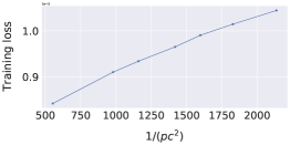
Refer to caption
(a) constant c𝑐c.
Refer to caption
(b) constant c𝑐c.
Refer to caption
(c) constant c𝑐c.
Refer to caption
(d) constant c𝑐c.
Refer to caption
(e) constant p𝑝p.
Refer to caption
(f) constant p𝑝p.
Figure 4: Impact of c𝑐c and p𝑝p on the convergence with the Gaussian stochastic noise σ2=1superscript𝜎21\sigma^{2}=1. The first four subfigures illustrate the impact of p𝑝p on convergence when c𝑐c is kept constant; showing a linear scaling of the loss compared to 1p1𝑝\frac{1}{p}. The last subfigure varies c𝑐c in the graph while keeping p𝑝p as a constant, and we see a linear scaling compared to 1c21superscript𝑐2\frac{1}{c^{2}}.

C.4 Additional Plots for Setup B
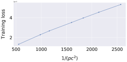
Refer to caption
(a) constant c𝑐c.
Refer to caption
(b) constant c𝑐c.
Refer to caption
(c) constant c𝑐c.
Refer to caption
(d) constant c𝑐c.
Refer to caption
(e) constant p𝑝p.
Refer to caption
(f) constant p𝑝p.
Figure 5: Impact of c𝑐c and p𝑝p on convergence with the structured stochastic noise σ2=1superscript𝜎21\sigma^{2}=1. The first four subfigures illustrate the impact of p𝑝p on convergence when c𝑐c is kept constant; showing a linear scaling of the loss compared to 1p1𝑝\frac{1}{p}. The last subfigure varies c𝑐c in the graph while keeping p𝑝p as a constant, and we can see a linear scaling compared to 1c21superscript𝑐2\frac{1}{c^{2}}.

In Figures 4 and 5 we study the impact of c𝑐c and p𝑝p on the convergence. These findings support the 𝒪(γ2σ2pc2)𝒪superscript𝛾2superscript𝜎2𝑝superscript𝑐2\mathcal{O}\left(\frac{\gamma^{2}\sigma^{2}}{pc^{2}}\right) scaling predicted by theory—however, cannot replace a formal proof. We leave this for future work.