– Under Review
\jmlryear2022
\jmlrworkshopFull Paper – MIDL 2022 submission
\DeclareMathOperator*\argmaxarg max
\DeclareMathOperator*\argminarg min
\midlauthor
\NameFelix Meissen\nametag1,2 \Emailfelix.meissen@tum.de
\addr1 Technical University of Munich, Germany
\addr2 Klinikum Rechts der Isar, Munich, Germany
\NameBenedikt Wiestler\nametag2 \Emailb.wiestler@tum.de
\NameGeorgios Kaissis\nametag1,2,3 \Emailg.kaissis@tum.de
\addr3 Imperial College London, UK
\NameDaniel Rueckert\nametag1,2,3 \Emaildaniel.rueckert@tum.de
On the Pitfalls of Using the Residual Error as Anomaly Score
Abstract
Many current state-of-the-art methods for anomaly localization in medical images rely on calculating a residual image between a potentially anomalous input image and its (\sayhealthy) reconstruction. As the reconstruction of the unseen anomalous region should be erroneous, this yields large residuals as a score to detect anomalies in medical images. However, this assumption does not take into account residuals resulting from imperfect reconstructions of the machine learning models used. Such errors can easily overshadow residuals of interest and therefore strongly question the use of residual images as scoring function. Our work explores this fundamental problem of residual images in detail. We theoretically define the problem and thoroughly evaluate the influence of intensity and texture of anomalies against the effect of imperfect reconstructions in a series of experiments. Code and experiments are available under \urlhttps://github.com/FeliMe/residual-score-pitfalls.
keywords:
Anomaly Segmentation, Semi-supervised Learning1 Introduction
Semi-supervised anomaly segmentation has shown great successes in the last years, for example in industrial defect detection Bergmann et al. (2019). Acquiring labels in medical images is both expensive (labeling oftentimes has to be performed by trained doctors) and inherently noisy due to inter-rater variability. Detecting pathologies in images without the need for labels would consequently be of great value in the medical domain, which led to increased research interest in this direction. In large medical 3D scans, a simple per-scan binary detection is not enough, as it would still require a professional to localize the anomaly. Ergo, accurate localization of pathologies is a necessity for clinical applicability in this domain. Usually, anomaly segmentation approaches for medical images train a generative model to learn the distribution of \sayhealthy images without visible pathologies. After training on such data, the model will likely fail to generate parts of the image that contain (out-of-distribution) pathologies and replace it with \sayhealthy (in-distribution) anatomy instead. In many cases, the pixel-wise residual between the original and the input image is used as a score to detect anomalous regions in the image. However, the results of Meissen et al. (2021) suggest that the approaches using this principle so far have only proven to be \saywhite object detection methods. On the other hand, unsupervised anomaly segmentation has potentially many applications in the medical domain where the pixel intensities of anomalies are similar to those of healthy pixels, such as colonoscopy images (Tian et al., 2021), Chest X-rays, or ultrasound images (Tan et al., 2021). Having anomaly segmentation methods for this kind of data would consequently be of great value. The results of the Medical Out-of-Distribution Analysis Challenge 2020 Zimmerer et al. (2020) also show that anomaly segmentation does not produce clinically usable results yet.
Contribution
In this work, we theoretically and experimentally evaluate the use of the pixel-wise residual error as a score for detecting anomalous regions in grayscale images. We simulate anomalies with specific characteristics on brain MR images and study the influence of anomaly texture, size, and their contrast to the surrounding tissue on the detection performance. We identify blind spots of this scoring metric and their causes.
2 Background and Related Work
The approaches for pixel-wise anomaly segmentation using residuals in medical grayscale images can be divided into two main categories:
Reconstruction-based Methods
An Autoencoder-like model, trained on \sayhealthy data only, computes a reconstruction from an input image . The anomaly map is the pixel-wise residual between and
| (1) |
where can also be an approximation of an expectation as in variational Autoencoders. Pawlowski et al. (2018) trained different Autoencoders – including a denoising Autoencoder and a variational Autoencoder – to detect anomalous regions in the form of tumors in CT images of the human brain. Baur et al. (2020a) used a UNet-like Autoencoder to detect MS lesions and glioblastoma in brain MRI. Their model produces higher-fidelity reconstructions than vanilla- or variational Autoencoders. However, they acknowledge that their method only works for hyperintense anomalies.
Restoration-based Methods
use a generative model – such as a VAE or a GAN – that have a smooth, interpolable latent space , such that latent vectors that are close in the latent space are also close in the image space . For a query image , they iteratively move along the latent manifold to find a generated image that is close to , but is still in the learned normative distribution. Restoration finds
| (2) |
via gradient descent. This method was originally proposed by Schlegl et al. (2017) with a Generative Adversarial Network (GAN). You et al. (2019) implemented another restoration variant that directly optimizes the pixels of the input image to maximize the ELBO of a VAE or a Gaussian Mixture VAE. Restoration-based approaches use iterative updating and are therefore orders of magnitude slower than reconstruction-based methods. Step size, number of optimization steps, and regularization-choice, and strength are additional hyper-parameters that need to be considered when using restoration.
For a more thorough investigation into the aforementioned categories, we refer the reader to the comparative study of Baur et al. (2021). Lastly, Meissen et al. (2021) did not train a machine learning model at all but used the histogram equalized input images directly as anomaly maps without computing a residual. This method by design can only detect hyperintense anomalies, but outperformed most competing methods on several benchmark datasets for lesion and tumor detection in brain MRI. Their results suggest that the competing methods themselves are merely \saywhite object detection methods that flag any hyperintense part of the image as anomalous.
3 Preliminaries and Notation
Assume we have a generative model that has learned the normative distribution perfectly, and will always generate \sayhealthy anatomy only.
Let be a query image with an anomalous region indexed by . Generative machine learning models can in practice not reconstruct images perfectly. Even for in-distribution images the error is not uniformly distributed over all pixels, but is larger at some parts of the image (i.e. at edges).
Let be the ground truth \sayhealthy query image. The magnitude of the anomaly map at pixels is bounded by . Consequently, if for any pixel outside of the anomaly , , then errors will be introduced.
4 Experiments
In this section, we present a series of experiments that investigate the limitations of using the pixel-wise residual error as a score to segment anomalies in grayscale images.
Data
We perform our experiments on the publicly available brain MRI data of the MOOD Analysis Challenge 2020 Zimmerer et al. (2020). It consists of 800 T2-weighted scans of healthy young adults with voxels per scan. The scans have voxel-intensities normalized between and , and the average intensity of non-zero voxels (voxels that are not part of the background) is . We split the data into a training and a test dataset, containing and of the scans respectively. We slice each scan into 2D images along the axial direction and select the 20 slices around the center for the training dataset and the center slice for the test dataset. For every image , we create its anomalous counterpart by sampling a circular patch, with a radius of pixels, at a random location inside the brain and altering the pixel values .
Evaluation Metric
In all our experiments, we use the pixel-wise average precision (AP) averaged over all images as the evaluation metric. AP is equivalent to the area under the precision-recall curve and is suited for measuring anomaly segmentation performance because the anomaly maps aren’t discrete segmentations, but continuous heatmaps.
4.1 Experiment 1 — Evaluating the Influence of Anomaly Intensity
fig:experiment1\subfigure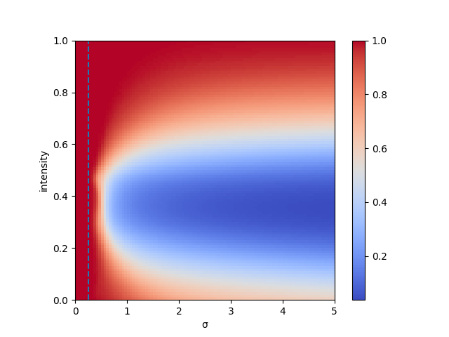 \subfigure
In the first experiment, we take a random healthy image from the test dataset. To create the anomalous image , we sample , as described in Section 4, and replace the pixel values in with an intensity between and . We simulate an Autoencoder that can perfectly remove the anomaly from , but generates imperfect reconstructions by applying Gaussian blur with between and to the healthy image: . We compute the pixel-wise anomaly map according to \equationrefeq:anomaly_map. This experiment is repeated for every image in the test dataset. The averaged results are shown in \figurereffig:experiment1_heatmap.
Findings
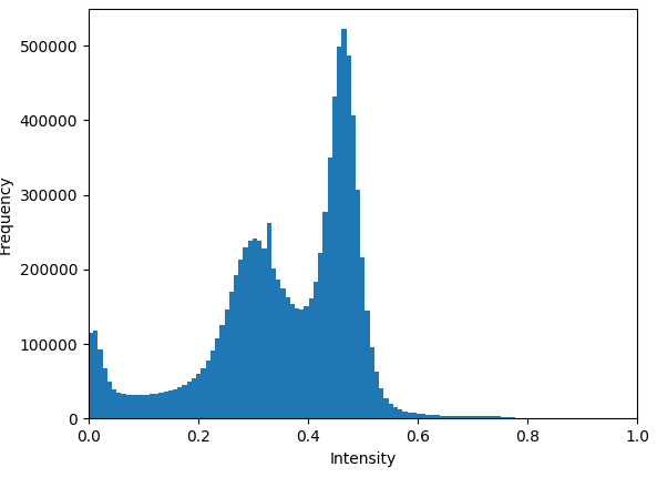
Average precision decreases heavily (already at small -values) when the anomalies have intensities between and . This indicates a large blind spot of the residual-based anomaly segmentation around the average pixel intensity of the object. The higher average precision for anomalies with high intensities can partly be explained by the histogram in \figurereffig:histogram. Only a few pixels in the test dataset have values , so the residual is likely to be high for these anomalies. Note that Gaussian blur starts having a noticeable effect on pixels when . Otherwise, more than of the Gaussian probability mass are on the center pixel, so little to no blurring occurs.
4.2 Experiment 2 — Evaluating the Influence of Anomaly Texture
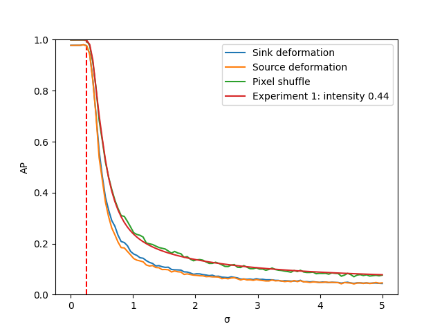
After examining the effect of the intensity of the anomalous regions in experiment 1, the following experiment will investigate the effect of their texture. Just like in experiment 1, we are simulating a generator with imperfect reconstructions using Gaussian blurring of the healthy image: . We again fix the anomaly size to 20 pixels and use three types of artificial anomalies that change the texture of the anomalous region but apply at most minimal changes to the overall intensity:
-
•
Sink deformation Tan et al. (2020): Pixels in the anomalous region with size get shifted away from the center of the region . In the new image , the pixel at index is replaced by the pixel from the original image at index : , , where , , and .
-
•
Source deformation Tan et al. (2020): Analogous to sink deformation, but pixels get shifted towards the center, so .
-
•
Pixel shuffle: The anomalous image is generated by randomly permuting all pixel indices in .
fig:experiment2
Findings
The results in \figurereffig:experiment2 show a lower performance for sink- and source deformation. The results for the pixel shuffle anomaly align closely to that of using a constant intensity of from experiment 1. Note that this value roughly equals the average intensity of brain pixels in the test dataset. These results indicate that the texture of the anomaly is not important for anomaly segmentation using the reconstruction error. Even when an extreme texture difference is applied, the performance is equivalent to applying no texture at all.
4.3 Experiment 3 — Transferring to Generative Machine Learning Models
Now that we described the AP landscape in experiments 1 and 2, experiment 3 will test the validity of the assumption that a generative model can be simulated by applying Gaussian blurring to the healthy image . For this experiment, we train multiple generative models on the training dataset. We train vanilla and spatial Autoencoders Baur et al. (2019) with varying latent space dimensions, and a hierarchical VQ-VAE Razavi et al. (2019) which is known to produce high-quality reconstructions. The vanilla and spatial Autoencoders all share the same encoder and decoder architecture with five layers. The VQ-VAE uses the original architecture and, therefore, has the largest latent space with dimensions. Architecture- and Training details can be found in the supplementary material.
4.3.1 Experiment 3.1
For the first sub-experiment, we generate the anomalous () and the healthy image () from the test dataset analogous to experiment 1. We use the trained model to generate a reconstruction of the healthy image , and again compute the anomaly map according to \equationrefeq:anomaly_map. This setup again assumes that the generator only produces \sayhealthy anatomy, but with reconstruction imperfections. The results are depicted in \figurereffig:experiment3.1. In addition to the AP curves of the single models, the Figure also contains the curves with the best matching from experiment 1 for the VQ-VAE, and the vanilla Autoencoder with . The best matching curves are the ones with the least absolute error to the AP curve of the respective model.
fig:experiment3\subfigure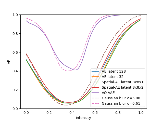 \subfigure
Findings
The experiment produces curves similar to the ones from experiment 1, both showing a significant drop in performance at intensities around . The performance of the VQ-VAE is similar to blurring the input image with , and the performance of the vanilla Autoencoders to blurring with . The Autoencoders with larger latent space (more capacity) produce better reconstructions and, thus, have a slightly better performance in this experiment.
4.3.2 Experiment 3.2
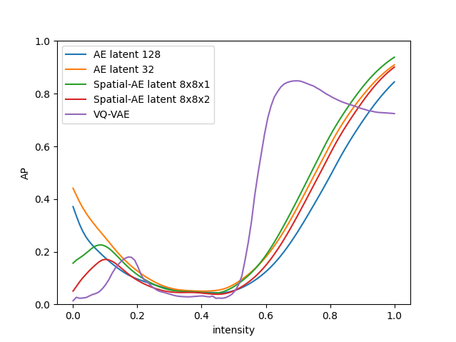
The second sub-experiment is performed analogous to the first one, with the difference that is the reconstruction of the anomalous image . This setup is more realistic since it does not rely on the assumption that the generator produces only \sayhealthy images.
fig:rec_err\subfigure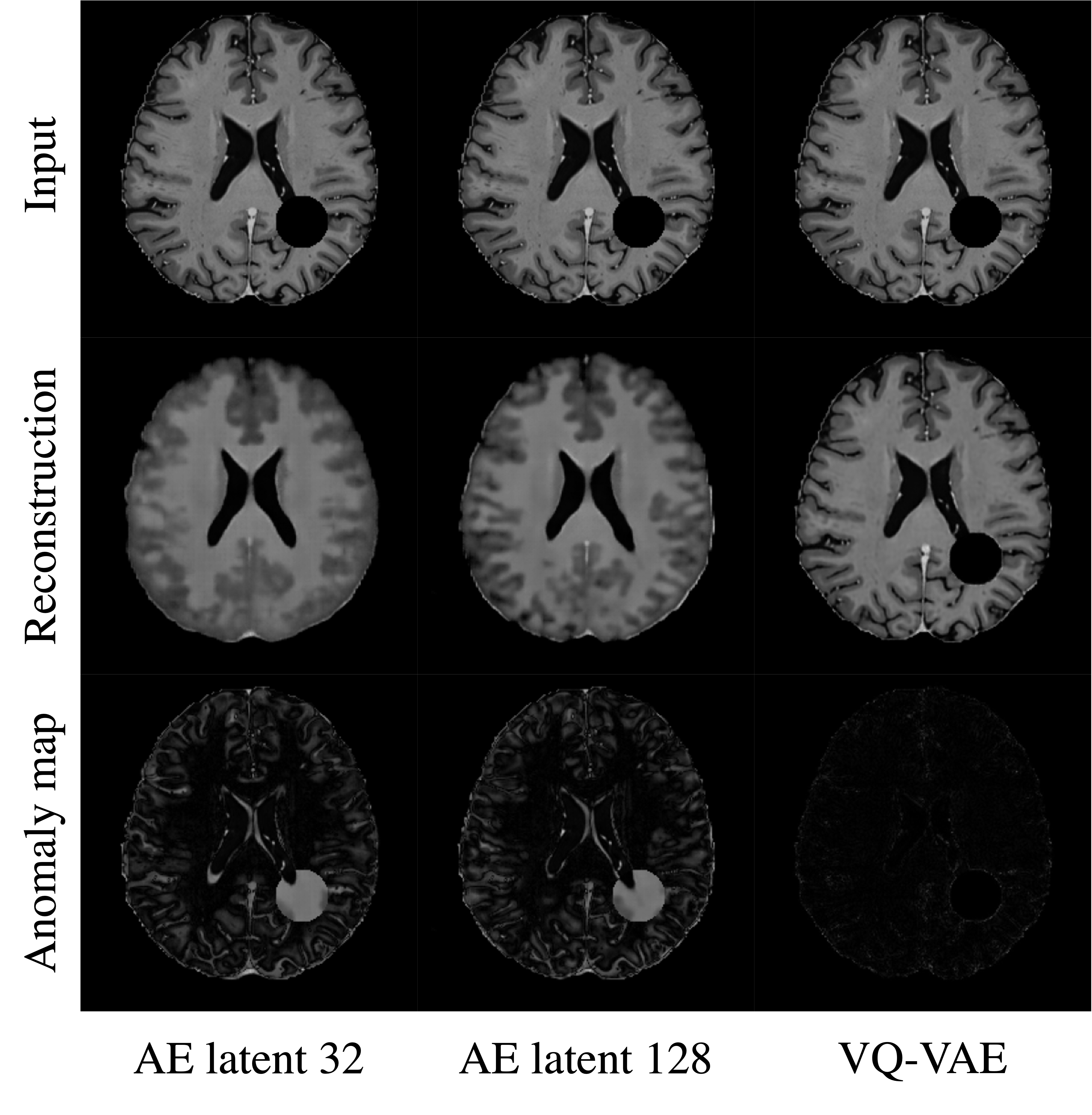 \subfigure
Findings
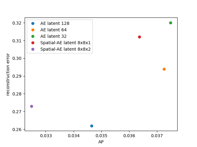
The results in \figurereffig:experiment3.2 show a reversed ordering of the AP-curves for vanilla Autoencoders. Here, models with larger latent space perform worse. The VQ-VAE drops most dramatically in performance compared to experiment 3.1. While its AP is still high for high-intensity anomalies, it drops fast and is especially low in the area of lower intensities. \figurereffig:samples explains this behavior. Models with lower reconstruction error tend to also reconstruct anomalies. This is well pronounced in the VQ-VAE, but can already be observed in the Vanilla AE where the reconstructed image of the larger model (latent space dimension of 128) has a slightly enlarged left lateral ventricle in the ventral aspect. \figurereffig:ap_vs_rec_err shows that models with a lower reconstruction error on the test dataset tend to show inferior anomaly segmentation performance.
The spatial Autoencoders and the VQ-VAE show a slight performance increase in \figurereffig:experiment3.2 around the intensity . We hypothesize that this is due to the pixel probability being low around this intensity in the test dataset as shown in \figurereffig:histogram. Thus, the residual is likely to be higher in this region. The same hypothesis explains the strong performance of all models on high-intensity anomalies.
5 Discussion
Above, we performed a series of experiments to investigate the influence of certain anomaly characteristics (such as intensity and texture) on the performance of using the pixel-wise reconstruction error as a score to segment anomalies in medical grayscale images. Our work uncovers severe problems with this method.
In Section 4.1, we discovered a large blind spot for anomalies with intensities around to , which corresponds roughly to the intensity range that is well covered by the pixels in the object as shown in \figurereffig:histogram, ergo in the area where the probability of finding , such that , is high. Considering this, the blind spot might be even larger for data that covers a broader intensity range. Additional experiments in this direction can be found in the Appendix. We further found in Section 4.2 that the important characteristic for anomalies to be detected is their intensity. Their texture, however, is irrelevant. While we found in experiment 3.1 (Section 4.3.1) that the assumption to simulate a machine learning generator with a Gaussian blurring process is reasonable, Section 4.3.2 made clear that performance can not trivially be increased by generating higher-quality images. In fact, increasing the model’s reconstruction quality leads to anomalies being reconstructed as well, which further hinders their detection and argues against this simple strategy. The same behavior was analyzed in the comparative study of Baur et al. (2021). They even found a positive correlation between the reconstruction error of normal pixels and the segmentation performance. Overall, our findings are in-line with current research by Meissen et al. (2021) who found that machine learning models that use pixel-wise residuals as anomaly maps are simple \saywhite object detection methods. This work further provides an explanation for why anomaly segmentation in brain MRI was so far mainly successful in imaging sequences where the anomalies of interest are known to be hyperintense (Pawlowski et al., 2018; Atlason et al., 2019; Zimmerer et al., 2019; Chen and Konukoglu, 2018; Pinaya et al., 2021; Baur et al., 2020b). Since the anomalous pixels there would be primarily located on the right-hand side of the histogram in \figurereffig:histogram, the probability mass of normal pixels with a similar intensity is lower, and the residual error is, therefore, expected to be higher. Histograms supporting this claim can be found in the Appendix. However, as the type and therefore also the characteristics of potential pathologies are unknown beforehand, our selection of artificial anomalies is not representative for all real-world cases. For example, abnormal size of anatomical structure could be considered as an anomaly. Nevertheless, our experiments allow to draw conclusions about all pathologies that are expressed via intensity- or texture difference.
6 Conclusion and Future Research
This work has shown that using the pixel-wise residuals between a grayscale image and its reconstruction to localize anomalies has severe limitations. Especially anomalies with intensities that are well covered by other pixels in the object can not reliably be detected with this method, regardless of their texture. While the main reason for this phenomenon is imperfect reconstructions of the generator model, increasing reconstruction quality does not trivially increase performance, but oftentimes leads to anomalies being reconstructed as well, hindering their detection. The successes of these methods in industrial defect detection suggest that the problem is less severe in RGB images. In future work, we will therefore research how medical scans with multiple channels can be constructed and their effect on anomaly detection. Also, advanced post-processing of the residual maps as in Muñoz-Ramírez et al. (2021) can potentially alleviate this problem and presents an interesting direction for further research. Lately, self-supervised methods that use artificial anomalies for training became popular (Tan et al., 2020, 2021) and need further investigation. Lastly, promising research directions are likelihood-based models and methods based on latent space features, such as Bergmann et al. (2020), to obtain pixel-wise likelihood estimates.
References
- Atlason et al. (2019) H. E. Atlason, A. Love, S. Sigurdsson, V. Gudnason, and L. M. Ellingsen. Unsupervised brain lesion segmentation from mri using a convolutional autoencoder. Medical Imaging 2019: Image Processing, Mar 2019. 10.1117/12.2512953.
- Baur et al. (2019) C. Baur, B. Wiestler, S. Albarqouni, and N. Navab. Deep autoencoding models for unsupervised anomaly segmentation in brain mr images. In A. Crimi, S. Bakas, H. Kuijf, F. Keyvan, M. Reyes, and T. van Walsum, editors, Brainlesion: Glioma, Multiple Sclerosis, Stroke and Traumatic Brain Injuries, pages 161–169, Cham, 2019. Springer International Publishing. ISBN 978-3-030-11723-8.
- Baur et al. (2020a) C. Baur, B. Wiestler, S. Albarqouni, and N. Navab. Bayesian skip-autoencoders for unsupervised hyperintense anomaly detection in high resolution brain mri. In 2020 IEEE 17th International Symposium on Biomedical Imaging (ISBI), pages 1905–1909, 2020a. 10.1109/ISBI45749.2020.9098686.
- Baur et al. (2020b) C. Baur, B. Wiestler, S. Albarqouni, and N. Navab. Scale-space autoencoders for unsupervised anomaly segmentation in brain mri. In International Conference on Medical Image Computing and Computer-Assisted Intervention, pages 552–561. Springer, Cham, 2020b.
- Baur et al. (2021) C. Baur, S. Denner, B. Wiestler, N. Navab, and S. Albarqouni. Autoencoders for unsupervised anomaly segmentation in brain mr images: A comparative study. Medical Image Analysis, 69:101952, 2021. ISSN 1361-8415. https://doi.org/10.1016/j.media.2020.101952.
- Bergmann et al. (2019) P. Bergmann, M. Fauser, D. Sattlegger, and C. Steger. Mvtec ad — a comprehensive real-world dataset for unsupervised anomaly detection. In 2019 IEEE/CVF Conference on Computer Vision and Pattern Recognition (CVPR), pages 9584–9592, 2019. 10.1109/CVPR.2019.00982.
- Bergmann et al. (2020) P. Bergmann, M. Fauser, D. Sattlegger, and C. Steger. Uninformed students: Student-teacher anomaly detection with discriminative latent embeddings. 2020 IEEE/CVF Conference on Computer Vision and Pattern Recognition (CVPR), Jun 2020. 10.1109/cvpr42600.2020.00424. URL \urlhttp://dx.doi.org/10.1109/CVPR42600.2020.00424.
- Carass et al. (2017) A. Carass, S. Roy, A. Jog, J. L. Cuzzocreo, E. Magrath, A. Gherman, J. Button, J. Nguyen, F. Prados, C. H. Sudre, and et al. Longitudinal multiple sclerosis lesion segmentation: Resource and challenge. NeuroImage, 148:77–102, 2017. ISSN 1053-8119. https://doi.org/10.1016/j.neuroimage.2016.12.064. URL \urlhttps://www.sciencedirect.com/science/article/pii/S1053811916307819.
- Chen and Konukoglu (2018) X. Chen and E. Konukoglu. Unsupervised detection of lesions in brain mri using constrained adversarial auto-encoders. In MIDL 2018 Conference book. MIDL, Jul 2018. https://doi.org/10.3929/ethz-b-000321650.
- Kuijf et al. (2019) H. J. Kuijf, A. Casamitjana, D. L. Collins, M. Dadar, A. Georgiou, M. Ghafoorian, D. Jin, A. Khademi, J. Knight, H. Li, and et al. Standardized assessment of automatic segmentation of white matter hyperintensities and results of the wmh segmentation challenge. IEEE Trans. Med. Imaging, 38(11):2556–2568, Nov 2019. ISSN 1558-254X. 10.1109/tmi.2019.2905770.
- Lesjak et al. (2018) Z. Lesjak, A. Galimzianova, A. Koren, M. Lukin, F. Pernuš, B. Likar, and Z. Spiclin. A novel public mr image dataset of multiple sclerosis patients with lesion segmentations based on multi-rater consensus. Neuroinformatics, 16, 01 2018. 10.1007/s12021-017-9348-7.
- Loshchilov and Hutter (2017) I. Loshchilov and F. Hutter. Decoupled weight decay regularization. arXiv preprint arXiv:1711.05101, 2017.
- Meissen et al. (2021) F. Meissen, G. Kaissis, and D. Rueckert. Challenging current semi-supervised anomaly segmentation methods for brain mri. arXiv preprint arXiv:2109.06023, 2021.
- Menze et al. (2015) B. H. Menze, A. Jakab, S. Bauer, J. Kalpathy-Cramer, K. Farahani, J. Kirby, Y. Burren, N. Porz, J. Slotboom, R. Wiest, and et al. The multimodal brain tumor image segmentation benchmark (brats). IEEE Trans. Med. Imaging, 34(10):1993–2024, 2015. 10.1109/TMI.2014.2377694.
- Muñoz-Ramírez et al. (2021) V. Muñoz-Ramírez, N. Pinon, F. Forbes, C. Lartizen, and M. Dojat. Patch vs. global image-based unsupervised anomaly detection in mr brain scans of early parkinsonian patients. Machine Learning in Clinical Neuroimaging, page 34–43, 2021. ISSN 1611-3349. 10.1007/978-3-030-87586-2_4. URL \urlhttp://dx.doi.org/10.1007/978-3-030-87586-2_4.
- Paszke et al. (2019) A. Paszke, S. Gross, F. Massa, A. Lerer, J. Bradbury, G. Chanan, T. Killeen, Z. Lin, N. Gimelshein, and L. et al. Antiga. Pytorch: An imperative style, high-performance deep learning library. In Advances in Neural Information Processing Systems 32, pages 8024–8035. Curran Associates, Inc., 2019. URL \urlhttp://papers.neurips.cc/paper/9015-pytorch-an-imperative-style-high-performance-deep-learning-library.pdf.
- Pawlowski et al. (2018) N. Pawlowski, M. C.H. Lee, M. Rajchl, S. McDonagh, E. Ferrante, K. Kamnitsas, S. Cooke, S. Stevenson, A. Khetani, T. Newman, and et al. Unsupervised lesion detection in brain ct using bayesian convolutional autoencoders. In MIDL 2018 Conference book. MIDL, April 2018.
- Pinaya et al. (2021) W. H. L. Pinaya, P. D. Tudosiu, R. Gray, G. Rees, P. Nachev, S. Ourselin, and M. J. Cardoso. Unsupervised brain anomaly detection and segmentation with transformers. arXiv preprint arXiv:2102.11650, 2021.
- Razavi et al. (2019) A. Razavi, A. van den Oord, and O. Vinyals. Generating Diverse High-Fidelity Images with VQ-VAE-2. Curran Associates Inc., Red Hook, NY, USA, 2019.
- Schlegl et al. (2017) T. Schlegl, P. Seeböck, S. Waldstein, U. Schmidt-Erfurth, and G. Langs. Unsupervised anomaly detection with generative adversarial networks to guide marker discovery. pages 146–157, 03 2017. ISBN 978-3-319-59049-3. 10.1007/978-3-319-59050-9_12.
- Tan et al. (2020) J. Tan, B. Hou, J. Batten, H. Qiu, and B. Kainz. Detecting outliers with foreign patch interpolation. arXiv preprint arXiv:2011.04197, 2020.
- Tan et al. (2021) J. Tan, B. Hou, T. Day, J. Simpson, D. Rueckert, and B. Kainz. Detecting outliers with poisson image interpolation. In M. de Bruijne, P. C. Cattin, S. Cotin, N. Padoy, S. Speidel, Y. Zheng, and C. Essert, editors, Medical Image Computing and Computer Assisted Intervention – MICCAI 2021, pages 581–591, Cham, 2021. Springer International Publishing. ISBN 978-3-030-87240-3.
- Tian et al. (2021) Y. Tian, G. Pang, F. Liu, Y. Chen, S. H. Shin, J. W. Verjans, R. Singh, and G. Carneiro. Constrained contrastive distribution learning for unsupervised anomaly detection and localisation in medical images. In International Conference on Medical Image Computing and Computer-Assisted Intervention, pages 128–140. Springer, 2021.
- You et al. (2019) S. You, K. Tezcan, X. Chen, and E. Konukoglu. Unsupervised lesion detection via image restoration with a normative prior. In International Conference on Medical Imaging with Deep Learning – Full Paper Track, London, United Kingdom, 08–10 Jul 2019. URL \urlhttps://openreview.net/forum?id=S1xg4W-leV.
- Zimmerer et al. (2019) D. Zimmerer, F. Isensee, J. Petersen, S. Kohl, and K. Maier-Hein. Unsupervised anomaly localization using variational auto-encoders. In Medical Image Computing and Computer Assisted Intervention – MICCAI 2019, pages 289–297. Springer International Publishing, 2019. ISBN 978-3-030-32251-9.
- Zimmerer et al. (2020) D. Zimmerer, J. Petersen, G. Köhler, P. Jäger, P. Full, T. Roß, T. Adler, A. Reinke, L. Maier-Hein, and K. Maier-Hein. Medical out-of-distribution analysis challenge, March 2020. URL \urlhttps://doi.org/10.5281/zenodo.3784230.
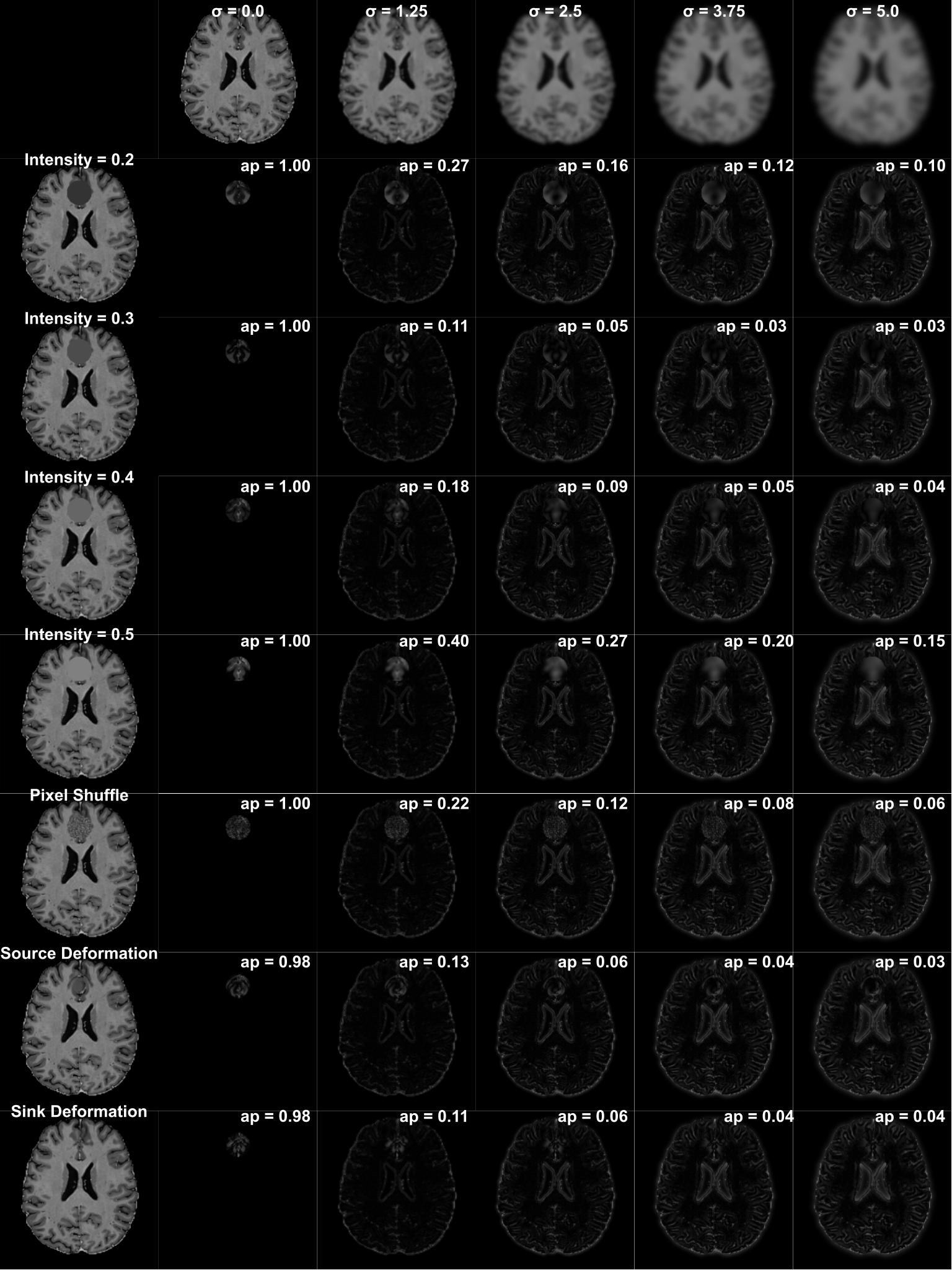
Appendix A Samples of Anomalies and Residual Maps
fig:anomalies
Appendix B Architecture and Training Details
Here we describe the architectures of the machine learning models used in our experiments.
B.1 Model Architectures
Vanilla Autoencoder
This model has a classical encoder-decoder structure with a latent bottleneck. The encoder consists of five downsampling layers, each with a convolutional layer with stride two and same padding, followed by batch normalization and a leaky ReLU activation function. The output of the encoder has the shape and is flattened before a fully connected layer transforms it into the latent vector of size . From there, another fully connected layer and a reshape operation transforms back to dimensions which is fed through the decoder. The decoder mirrors the encoder but uses Transpose Convolutions instead of regular ones. Lastly, a final Convolution is applied to the output of the decoder to generate the final reconstruction.
Spatial Autoencoder
The architecture of the spatial Autoencoder is analogous to the one of the vanilla Autoencoder. The only difference is the bottleneck where now a Convolution transforms the output of the decoder into , and another Convolution transforms this vector back to fit into the decoder. The latent space in these models is of shape and retains an image-like structure.
VQ-VAE
This model uses the original architecture proposed in Razavi et al. (2019) for image resolutions of . Apart from the bottleneck, this model differs from the others by using residual blocks in the encoder and decoder and by having two latent spaces: one at resolution , and one at resolution , making it the largest latent space of all models considered.
B.2 Training details
We implemented all models using PyTorch (Paszke et al., 2019). All models are trained using the AdamW optimizer Loshchilov and Hutter (2017) with a learning rate of for steps with a batch size of to minimize the L1 loss between the input image and its reconstruction. During training, we use of the training dataset for validation. When training the VQ-VAE, we weighted the latent loss by a factor of compared to the reconstruction error.
Appendix C Experiment 1 with Histogram Equalization
Here, we perform an additional experiment, investigating the hypothesis from Section 5 that the blind-spot of the residual error might be larger when the data covers a broader intensity range. For this, we repeat experiment 1 with histogram-equalized data. Specifically, we perform histogram equalization to each image slice in the test dataset, and only to pixels in the image that belong to the brain.
fig:experiment1_histequal\subfigure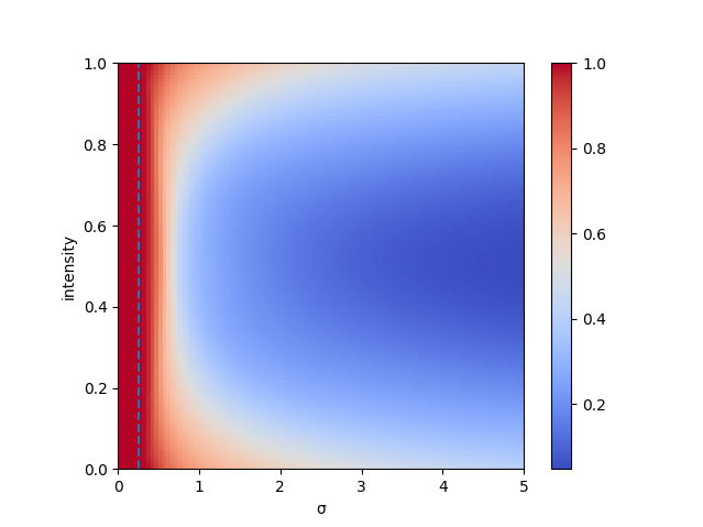 \subfigure
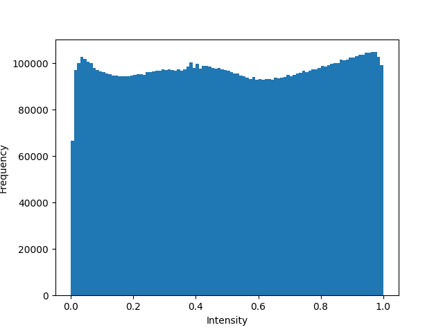
The results, alongside the histogram of the equalized data can be found in \figurereffig:experiment1_histequal. The performance drop is now distributed symmetrically over the whole intensity range, confirming our initial hypothesis.
Appendix D Histograms of Brain MRI Datasets
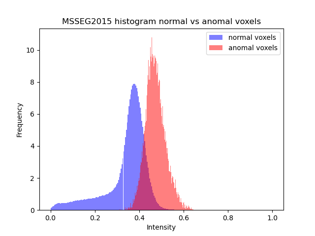
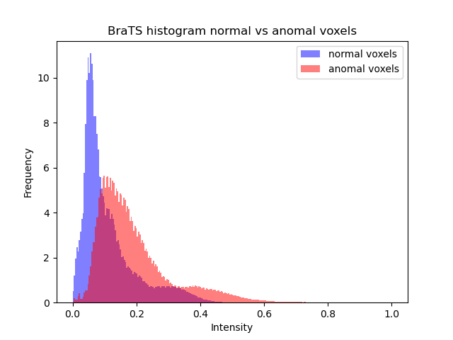
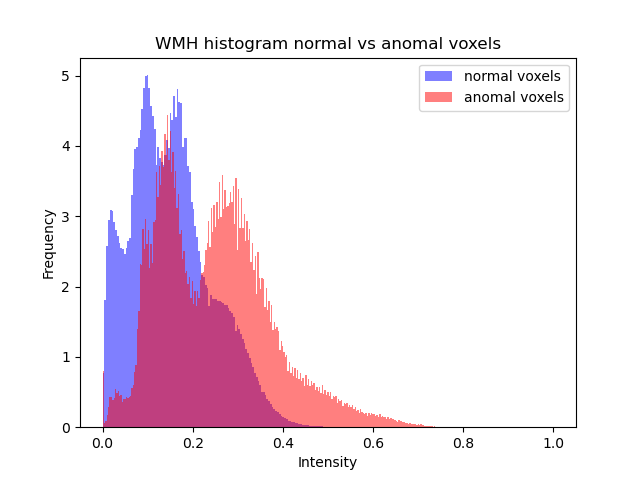
Here, we show the histograms of normal and anomal voxels of four data sets commonly used to evaluate anomaly segmentation for brain MRI. In all data sets the intensities of anomal voxels tend to be higher then the intensities of normal voxels.
fig:brats_mslub_hist
\subfigure
 \subfigure
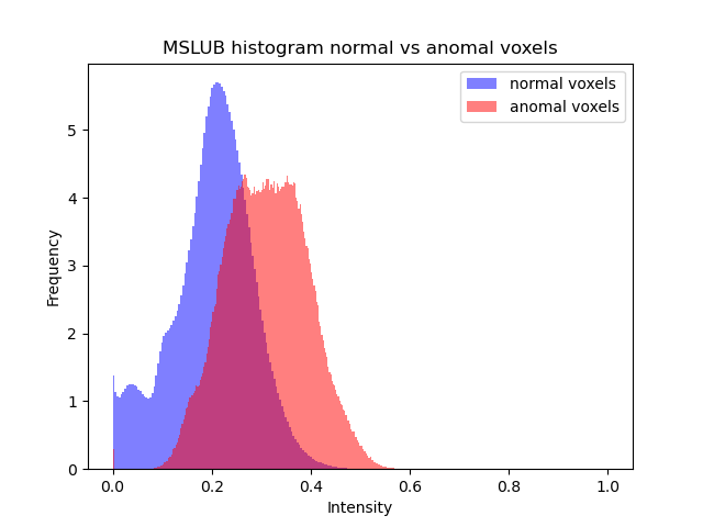
fig:wmh_msseg_hist
\subfigure
 \subfigure
