A Unified Prediction Framework for Signal Maps

Abstract.

Signal maps are essential for the planning and operation of cellular networks. However, the measurements needed to create such maps are expensive, often biased, not always reflecting the performance metrics of interest, and posing privacy risks. In this paper, we develop a unified framework for predicting cellular performance maps from limited available measurements. Our framework builds on a state-of-the-art random-forest predictor, or any other base predictor. We propose and combine three mechanisms that deal with the fact that not all measurements are equally important for a particular prediction task. First, we design quality-of-service functions ($Q$), including signal strength (RSRP) but also other metrics of interest to operators, such as number of bars, coverage (improving recall by 76%-92%) and call drop probability (reducing error by as much as 32%). By implicitly altering the loss function employed in learning, quality functions can also improve prediction for RSRP itself where it matters (e.g., MSE reduction up to 27% in the low signal strength regime, where high accuracy is critical). Second, we introduce weight functions ($W$) to specify the relative importance of prediction at different locations and other parts of the feature space. We propose re-weighting based on importance sampling to obtain unbiased estimators when the sampling and target distributions are different. This yields improvements up to 20% for targets based on spatially uniform loss or losses based on user population density. Third, we apply the Data Shapley framework for the first time in this context: to assign values ($\phi$) to individual measurement points, which capture the importance of their contribution to the prediction task. This can improve prediction (e.g., from 64% to 94% in recall for coverage loss) by removing points with negative values, and can also enable data minimization (i.e., we show that we can remove 70% of data w/o loss in performance). We evaluate our methods and demonstrate significant improvement in prediction performance, using several real-world datasets.

1. Introduction

Cellular operators rely on key performance indicators (a.k.a. KPIs) to understand the performance and coverage of their network, as well as that of their competitors, in their effort to provide the best user experience. KPIs usually include wireless signal strength measurements (e.g., LTE reference signal received power, a.k.a. RSRP), other performance metrics (e.g., throughput, delay) and information associated with the measurement (e.g., frequency band, location, time, call drop probability etc.). Cellular performance maps (a.k.a. signal maps) consist of a large number of KPIs in several locations; an example is depicted on Fig. 2. They are of immense importance to operators for planning, managing and upgrading their networks.

Traditionally, cellular operators collected such measurements by hiring dedicated vans (a.k.a. wardriving (Yang et al., 2010)) with special equipment, to drive through, measure and map the received signal strength (RSS) in a particular area of interest. However, in recent years they increasingly outsource the collection of signal maps to third parties (Alimpertis et al., 2019). Mobile analytics companies, such as OpenSignal (Open Signal Inc., 2011) and Tutela (Tutela Inc., 2011), crowdsource measurements directly from end-user devices, via standalone mobile apps, or measurement SDKs integrated into other apps, such as games, utilities or streaming apps. Either way, signal strength maps are expensive for both operators  and crowdsourcing companies to obtain, and may not be available for all locations, times, frequencies, and other parameters of interest. The upcoming dense deployment of small cells at metropolitan scales will only increase the need for accurate and comprehensive signal maps to enable 5G network management (Garcia-Reinoso et al., 2019; Imran et al., 2014).

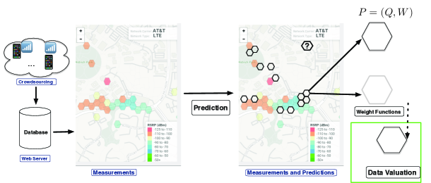
Figure 1. Overview of our framework: the goal is to predict cellular values $\hat{y}$, based on features $\mathbf{x}$, while training on available (and unequally important) measurements. As base workhorse ML model, we use our state-of-the-art RF-predictor (Sec. 3.2), but any other predictor would do as well. Our framework builds on top of the base predictor and deals with the different importance of data points in three distinct ways. (1) We use quality-of-service functions $Q$ to predict directly KPIs of interest; these depend on but are different from raw signal strength RSRP (Sec. 3.3). (2) We use weight functions $W$ to target the mismatch between sampling and target distributions (Sec. 3.4). (3) We apply the Data Shapley framework to assess the importance (i.e., predictive value) $\phi$ of the measurements w.r.t. the prediction task at hand $(P,W)$ (Sec. 3.5).

For these reasons, there has been significant interest in signal map prediction techniques based on a limited number of spatiotemporal cellular measurements. These include propagation models (Yun and Iskander, 2015; Bultitude and Rautiainen, 2007), data-driven approaches (Fida et al., 2017; Chakraborty et al., [n.d.]; He and Shin, 2018) and combinations thereof (Phillips et al., 2012). Increasingly sophisticated machine learning models are being developed to capture various spatial, temporal and other characteristics of signal strength (Ray et al., 2016; Enami et al., 2018; Alimpertis et al., 2019) and throughput (Wang et al., 2017; Zhang and Patras, 2018). Prior work has focused exclusively on minimizing the mean squared error (MSE) in predictions of raw signal strength (RSRP). In our prior work  (Alimpertis et al., 2019), we developed a Random Forests (RFs)-based predictor, and we showed that it outperforms state-of-the-art RSRP predictors. In this paper, we use this RFs-predictor as our base ”workhorse” ML model and we develop a framework on top of it, to deal with the fact that not all measurements are equally important.

We observe that three different factors affect the importance of measurement data points when those are used for training ML predictors. First, what KPI we predict: operators are typically interested in performance metrics such as coverage, call drop probability, number of bars; these depend on but go beyond raw signal strength (RSRP). Second, where we make the prediction: the operators may be interested in predicting performance better in some locations (e.g., those with weak coverage or at important sites), while they may have no control on how crowdsourced mobile measurements are distributed. Third, since measurements are expensive and may pose privacy risks, we may want to identify those data points with the highest predictive value and discard outliers or redundant measurements.

In order to address the aforementioned challenges, we develop a unified framework for predicting cellular performance maps, which provides cellular operators and mobile analytics companies with knobs to express and deal with the unequal importance of available cellular measurements. We define two classes of functions $Q$ and $W$, that jointly define the performance of the signal maps prediction problem $P=(Q,W)$. These functions tackle the mismatch between: (1) the operators’ quality (QoS) metrics of interest and the raw signal strength (RSRP) and (2) the sampling and target distributions, respectively. In addition, (3) we compute the data Shapley values ($\phi$) of measurement data points that capture their importance for training a predictor for the particular cellular map prediction problem $P=(Q,W)$ at hand. Our three contributions are summarized on Fig. 1 and are further elaborated upon next.

(1) Quality Functions $Q$. We consider quality-of-service functions ($Q$), based on signal strength, which specify what metric operators and users care about, such as mobile coverage indicators ($Q_{c}$), call drop probability ($Q_{CDP}$), and number of bars ($Q_{B}$). Prior work exclusively minimizes the MSE for signal strength (RSRP)  (Enami et al., 2018; Fida et al., 2017; He and Shin, 2018; Phillips et al., 2012), which does not directly optimize prediction for the aforementioned metrics. In contrast, we show that learning directly on the $Q$ domain can significantly improve performance vs. state-of-the art, including: (i) recall gains from 76% to 92% and balanced accuracy gains from 87% to 94% for predictions of coverage loss (where false negatives are costly to operators); and (ii) reductions in relative error in predicted CDP by up to 32% (in the high CDP regime of greatest concern to cellular operators). Even for predicting signal strength (RSRP) itself, accuracy is often more critical in the low than in the high signal-strength regime. Specifying objectives via quality functions implicitly tunes the loss function, and allows operators to put more emphasis on values and use cases of signal maps that matter most. For example, we show improvement of prediction of RSRP itself in the low signal strength regime, of up to 27% ($3$dB in RMSE).

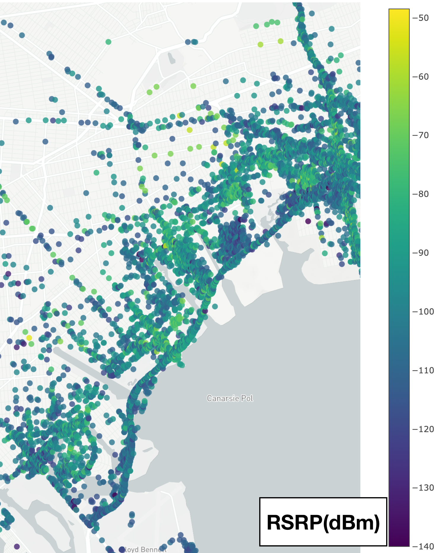
Figure 2. Example of a typical Signal Strength (RSRP) Map from the East NYC dataset, near the JFK airport.

(2) Weight functions $W$. Sampling bias is inherent in crowdsourced data due to the non-uniform population density, as well as the commute and usage patterns. An operator may be interested in knowing KPIs at particular locations (as well as times, frequencies, and other features). Examples of target locations of interest for prediction include: locations where there is poor coverage, locations with dense user population, origins of calls to 911 dispatchers, client sites during working hours. However, these target locations may differ from the sampling locations where measurements are available, thus optimization to available data can lead to biased inference. This mismatch of the sampling distribution with the target distribution is also known as the dataset shift problem (Snoek and et al., 2019) in ML. To tackle this mismatch, we propose a re-weighting method, rooted in the framework of importance sampling, which leads to unbiased error. We introduce weight functions ($W$) that allow operators to express where (e.g., in which particular locations, times, etc.) they are interested in predicting performance most accurately. We demonstrate improvement up to 20% for two intuitive target distributions: uniform loss across a spatial area and loss proportional to population density. Combining weight targeting and quality functions improves further, e.g., up to 5% more for estimating CDP on targeted spatial losses.

(3) Data Shapley $\phi$. We recognize and exploit the fact that not all measurements are equally important for predicting the metric of interest at the location of interest. We apply, for the first time in the context of signal maps, the Data Shapley framework, originally defined in economics and recently adapted to assign value to training data in ML (Ghorbani and Zou, 2019). Our Data Shapley framework takes as input the available cellular measurements, the ML prediction algorithm, and the error metric, re-weighted for the particular prediction problem $P=(Q,W)$; it then computes the Shapley values ($\phi$) of individual measurements used for training the ML model. This enables us to then remove measurements with negative or low data Shapely values (e.g., outliers or irrelevant for the specific task) that improves prediction, and can also guide data minimization (thus improve privacy). For example, we show that we can remove up to 65-70% of data points, while simultaneously improving the recall of cellular coverage indicator from 64% to 99%.

Throughout the paper, we leverage two types of large, real-world LTE datasets to gain insights and evaluate prediction performance: (i) a dense Campus dataset, we collected on our own university campus; and (ii) several sparser city-wide (in NYC and LA) datasets, provided by a mobile data analytics company.

The rest of the paper is organized as follows. Section 2 reviews related work. Section 3 presents our prediction framework, including the baseline predictor (Sec. 3.2) and the methodologies that deal with unequal importance of measurements, i.e., the quality functions (Sec. 3.3), the weight functions (Sec. 3.4), and the data valuation (Sec. 3.5). Section 4 presents evaluation results, based on the aforementioned datasets. Section 5 concludes the paper. The Appendix (in Supplemental Materials) provides details on the Data Shapley formulation (A1) and on the choice of the base predictor (A2).

2. Our Work in Perspective

Broadly speaking, signal strength can be predicted by propagation models or data-driven approaches, including geospatial interpolation, (e.g.,  (Fida et al., 2017; Phillips et al., 2012)) and machine learning (e.g.,  (Enami et al., 2018; Alimpertis et al., 2019)); or combinations thereof: (Phillips et al., 2012).

Propagation models. State-of-the-art propagation and path loss (equation-based) models include WINNER I/II (Bultitude and Rautiainen, 2007), Ray tracing (Yun and Iskander, 2015) and others. However, this family of models requires a detailed map of the environment and fine grained tuning of model’s parameters (Alimpertis et al., 2019). A simple yet widely used propagation model is LDPL (Alimpertis et al., 2014) and its indoor variant (Applegate et al., 2018).

Geospatial interpolation (Chakraborty et al., [n.d.]; Phillips et al., 2012; Fida et al., 2017). Methods such as Ordinary Kriging (OK) and OK Detrending (Phillips et al., 2012), which are used by the ZipWeave (Fida et al., 2017) and SpecSense (Chakraborty et al., [n.d.]) frameworks, cannot naturally incorporate additional features beyond location (such as time, frequency, hardware etc. ), as our ML models do (both in this paper and in our prior work (Alimpertis et al., 2019)).

Machine learning: DNNs. Examples of RSRP/RSS prediction include (Enami et al., 2018) and (He and Shin, 2018). Work in (Enami et al., 2018) uses DNNs along with detailed 3D maps from LiDAR and work in (He and Shin, 2018) uses Bayesian Compressive Sensing (BCS). ML models for the signal strength likelihood for user localization have also been developed by prior art (Ray et al., 2016; Margolies et al., 2017; Hähnel and Fox, 2006). Krijestorac et al. (Krijestorac et al., 2020) propose state-of-the-art CNNs for estimating signal strength values and utilize a 3D map of the environment as features. In particular, they treat signal strength as a Gaussian random variable and predict its mean and variance. The evaluation is based on simulated data via ray-tracing software, which allows continuous infill of regions. However, when trained and evaluated on real-world datasets, this approach faces the limitation of sparse data. (Teganya and Romero, 2020) uses autoencoders for predicting signal strength, but similarly their method is limited to simulated data.

Machine learning: Random Forests. In our prior work (Alimpertis et al., 2019), we proposed random forests (RFs) for predicting signal strength (RSRP) based on a number of features, including but not limited to location and time (see Section 3.2). We demonstrated that RFs can outperforms prior art (including model-based and geospatial methods) because they can inherently capture spatial and temporal correlations, while also naturally extending to features beyond location (geospatial predictors can only handle location features) (Alimpertis et al., 2019). For instance, for MSE minimization, the RFs  requires 80% less measurements for the same prediction accuracy, or reduces the relative error by 17% for the same number of measurements compared to geospatial interpolation methods used by ZipWeave (Fida et al., 2017) and SpecSense (Chakraborty et al., [n.d.]). In Section 4.3 and Appendix A2, we also compare RFs  to recent DNN and CNN-based predictors, and we show that RFs still outperform alternatives.

Other Metrics - Dealing with unequal importance. Recent work in QoS has considered how RSRP measurements could be used as proxy to predict Quality of Experience (QoE) (Adarsh et al., [n.d.]) or reinforcement-learning prediction techniques for video playback (Mao et al., 2017). Apart from signal strength, prior work considered mobile traffic volume maps (i.e., KPI throughput) (Zhang and Patras, 2018; Wang et al., 2017; Narayanan, 2020), but solely focusing on the underlying ML model and MSE minimization. Importance sampling for deep neural network training is considered in (Katharopoulos and Fleuret, 2018). The mismatch between sampling and target distributions is also related to the dataset shift problem (Snoek and et al., 2019) in machine learning.

Contributions. In this paper, we use our own implementation of RFs-predictor as a state-of-the-art “work horse” signal map predictor. For completeness, we present the method and its evaluation in Sec. 3.2 and Appendix 2. However, our focus here is orthogonal: we propose a framework that combines three methodologies ($Q,W,\phi$) to deal with the unequal importance of available measurements for a particular prediction problem $P=(Q,W)$. Our framework builds on top of RFs, but could also utilize any other underlying ML algorithm minimizing a squared-error loss. To the best of our knowledge, this is the first paper to leverage QoS to improve prediction of those metrics but also of RSRP itself in regimes where it matters; and to develop a ($Q,W$)-specific data Shapley valuation for data minimization and prediction improvement.

A summary of prior approaches for signal map prediction, and a quantitative comparison to our framework, is presented in Table 1. There is an increasing amount of work on mobile crowdsourced data privacy recently, with applications including signal strength, radiation maps, etc.  (Boukoros et al., 2019). In other work from our group (Bakopoulou et al., 2021), we have also considered distributed settings and privacy-utility tradeoffs. Location privacy is a large research area on its own and out-of-scope for this paper. Here we focus on optimizing prediction, in a centralized setting, given measurements of unequal importance. This being said, the data minimization enabled by the Shapley framework is a useful tool for improving privacy.

	Features				Environment, Scale, Data			Evaluation
	Spatial	Time	Device, Network	LiDar, 3D Maps Agnostic	Environment Agnostic	City Wide	Real Data	Quality Beyond RSRP
Log-Distance Path-Loss ($LDPL$)	$\color[rgb]{0,1,0}{\Huge\checkmark}$	X	X	$\color[rgb]{0,1,0}{\Huge\checkmark}$	$\color[rgb]{0,1,0}{\Huge\checkmark}$	X	$\color[rgb]{0,1,0}{\Huge\checkmark}$	X
COST-231/ WINNER I-II/ Ray Tracing	$\color[rgb]{0,1,0}{\Huge\checkmark}$	X	$\color[rgb]{0,1,0}{\Huge\checkmark}$	X	X	X	$\color[rgb]{0,1,0}{\Huge\checkmark}$	X
Geostatistics Specsense(Chakraborty et al., [n.d.])	$\color[rgb]{0,1,0}{\Huge\checkmark}$	X	X	$\color[rgb]{0,1,0}{\Huge\checkmark}$	X	X	$\color[rgb]{0,1,0}{\Huge\checkmark}$	X
BCS (He and Shin, 2018)	$\color[rgb]{0,1,0}{\Huge\checkmark}$	$\color[rgb]{0,1,0}{\Huge\checkmark}$	X	$\color[rgb]{0,1,0}{\Huge\checkmark}$	X	X	$\color[rgb]{0,1,0}{\Huge\checkmark}$	X
DNNs (RAIK (Enami et al., 2018))	$\color[rgb]{0,1,0}{\Huge\checkmark}$	X	X	X	X	$\color[rgb]{0,1,0}{\Huge\checkmark}$	$\color[rgb]{0,1,0}{\Huge\checkmark}$	X
CNNs (Krijestorac et al., 2020)	$\color[rgb]{0,1,0}{\Huge\checkmark}$	X	X	X	$\color[rgb]{0,1,0}{\Huge\checkmark}$	X	X	X
Auto- Encoders (Teganya and Romero, 2020)	$\color[rgb]{0,1,0}{\Huge\checkmark}$	X	X	X	$\color[rgb]{0,1,0}{\Huge\checkmark}$	X	X	X
Our Framework	$\color[rgb]{0,1,0}{\Huge\checkmark}$	$\color[rgb]{0,1,0}{\Huge\checkmark}$	$\color[rgb]{0,1,0}{\Huge\checkmark}$	$\color[rgb]{0,1,0}{\Huge\checkmark}$	$\color[rgb]{0,1,0}{\Huge\checkmark}$	$\color[rgb]{0,1,0}{\Huge\checkmark}$	$\color[rgb]{0,1,0}{\Huge\checkmark}$	$\color[rgb]{0,1,0}{\Huge\checkmark}$

Table 1. Comparison of our framework to other approaches for signal map prediction.

3. Prediction Framework

3.1. Signal Maps Prediction

3.1.1. Definitions and Problem Space

An observed signal map is a collection of $N$ measurements $(\mathbf{x_{i}},y_{i})$, $i=1,2...N$, where $y_{i}=\{$$y^{P}$, $y^{I}$, $y^{C}$$\}$ denotes the KPI of interest given the feature vector $\mathbf{x}_{i}$ (e.g., location etc.) w.r.t. which the signal is to be mapped. In general, an operator’s interest is not only in the observed signal strength map, but in an underlying “true” signal strength map, defined by the conditional distribution $Y|\mathbf{x}$ for an arbitrary $\mathbf{x}\in\mathbb{X}$, where $Y$ is the (generally unobserved) KPI at $\mathbf{x}$ and $\mathbb{X}$ specifies a region of interest (e.g., an areal unit, time period, etc.). This suggests approximation of the true signal strength map by machine learning (ML), where our goal is to answer queries regarding $Y|\mathbf{x}$, or functions thereof, by training a predictor on the observed data.

$y$: Key Performance Indicators (KPIs). There are many KPIs for LTE defined by 3GPP:

• RSRP ($y^{P}$): The reference signal received power is the average over multiple reference and control channels, reported in dBm. It is of great importance for LTE and utilized for cell selection, handover decisions, mobility measurements etc.

• RSRQ ($y^{I}$): The reference signal received quality is a proxy to measure channel’s interference.

• CQI ($y^{C}$): The channel quality indicator is a unit-less metric ($y^{C}$= $\{0,\cdots,15\}$) of the overall performance.

It is worth noting, that all prior work focused exclusively on predicting RSRP. Therefore, we use $y=\text{$y^{P}$}$, to refer to prediction of RSRP, unless otherwise noted.

$\mathbf{x}$: Measurement Features. For each measurement $i$ in our datasets, we use several features available via Android APIs (Alimpertis et al., 2019). $\mathbf{x_{i}^{full}}=(l_{i}^{x},l_{i}^{y},d,h,\text{$cID$},\text{$dev$},out,||\mathbf{l}_{BS}-\mathbf{l}_{i}||_{2},\text{$freq_{dl}$})$. We consider the following features:

• Location: $\mathbf{l}_{j}=(l_{i}^{x},l_{i}^{y})$: GPS’s latitude and longitude.

• Time: $\mathbf{t_{i}}=(d,h)$, where $d$ is the weekday and $h$ the hour the measurement was collected.

• Cell ID and LTE TA: KPIs are defined per serving LTE cell, which is uniquely identified by the CGI (cell global identifier, cell ID or $cID$) which is the concatenation of the following identifiers: the MCC (mobile country code), MNC (mobile network code), TAC (tracking area code) and the cell ID. LTE also defines Tracking Areas, LTE TA, by the concatenation of MCC, MNC and TAC, to describe a group of neighboring cells, under common LTE management.

• Device hardware type ($dev$): This refers to the device model (e.g., Galaxy s21 or iPhone 13) and not to device identifiers.

In (Alimpertis et al., 2019), we considered all features and showed the most important ones to be location, time, cell $cID$ and device hardware information $dev$. In this paper, we consider x to be the full set of features, unless otherwise noted.

	Notations	Definitions-Description
Data	$\mathbf{x}$	Measurement’s Features
	$y$	Label - KPI (Key Performance Indicator)
	$\{y^{P},y^{I},y^{C}\}$	KPIs in this Paper
	$y^{P}$	RSRP: Received Signal Reference Power
	$y^{I}$	RSRQ: Received Signal Reference Quality
	$y^{C}$	CQI: Channel Quality Indicator
Network Quality Functions	$Q(y)$	Network Quality Function
	$Q_{c}(y^{P})$	Mobile Coverage Indicator
	$Q_{cdp}(y)$	Call Drop Probability
Error / Loss Scores	$L(\widehat{y},y)$	Loss function; squared loss in this work
	$\varepsilon_{p}$	Reweighted Error Metric for Target $p(\mathbf{x})$
Importance Sampling Framework	$p(\mathbf{x})$	Target distribution
	$s(\mathbf{x})$	Sampling Distribution
	$d(\mathbf{x})$	Population Distribution
	$u(\mathbf{x})$	Unifom Distribution
	$W(\mathbf{x})$	Weighting Function
	$w_{u}$	Importance Ratio for Uniform $p(\mathbf{x})$
	$w_{d}$	Importance Ratio for Population $p(\mathbf{x})$

Table 2. Terminology and Notation.

Signal Map Prediction. Our goal is to predict an unknown signal map value $\hat{y}$ at a given location and other features ($\mathbf{x}\in\mathbb{X}$), based on available spatiotemporal measurements with labeled data $(\mathbf{x}_{i},y_{i})$, $i=1,...N$, either in the same $cID$ or in the same LTE TA. The real world underlying phenomenon is a complex process $y=f(\textbf{x})$ that depends on $\mathbf{x}$, and characteristics of the wireless environment.

It is important to consider the loss to be minimized by the choice of predictor: certain loss functions improve performance for certain objectives, while degrading it in others. We consider two factors relating to the choice of loss. First, an operators’ interest is not always in KPI $y$ itself, but in some quality of service function, $Q(y)$; see Section 3.3 for concrete examples. While conventional training schemes focus on predicting $y$ (e.g., w.r.t. mean squared error, or MSE), we consider signal map prediction that minimizes error in the predicted value of $Q(y)$ itself. We demonstrate that the nonlinear dependence of quality-of-service on raw signal strength makes this direct approach superior for many practical applications. Second, the operator may wish to weight accuracy for some values of $\mathbf{x}$ more heavily than others. While conventional training schemes implicitly assume that importance corresponds to data sampling frequency, we instead consider optimization w.r.t. an application-specific weight function $W(\mathbf{x})$ that may or may not closely correspond to the distribution of sampled observations; see Table 3 and Section 3.4 for details.

Training Options	$y$ Domain	$Q$ Domain
same $w=1$ for all points	$P_{B}=(I,k)$	$P=($$Q,k$$)$
	$\widehat{y}\rightarrow$ $Q(\widehat{y})$	$Q(y)\rightarrow\widehat{Q}(y)$
training weights $w$ (Table 3)	$P=($$I,W$$)$	$P=($$Q,W$$)$
	$\widehat{y_{w}}\rightarrow$ $Q(\widehat{y_{w}})$	$Q(y)\rightarrow\widehat{Q}^{w}(y)$

Table 3. Overview of prediction problems $P=(Q,W)$. One can perform prediction on the y (signal) or on the Q (quality) domain. One can assign the same or different weights to different points.

Prediction Problem Space: $P=(Q,W)$. With the above motivation, we may formalize the prediction problem as follows. Let $\mathbb{Y}$ be the space of potential KPI values. $Q\in\mathbb{Q}:\mathbb{Y}\mapsto\mathbb{R}$ is a quality function, as described above. Similarly, $W\in\mathbb{W}:\mathbb{X}\mapsto\mathbb{R}^{+}_{0}$ is the above described weight function. We define the prediction problem space as $\mathbb{P}=\mathbb{Q}\times\mathbb{W}$, whose elements $P=(Q,W)\in\mathbb{P}$ are prediction problems. This representation provides a simple unifying formalism for a range of different problems. For instance, note the base problem $P_{B}=(I,k)$ where $I$ is the identity function and $k$ is a constant function, which amounts to the conventional learning problem assumed in the prior literature. Here, we develop not only predictors which minimize loss under $P_{B}$, but also or other arbitrary $P\in\mathbb{B}$. In practice, this amounts to finding predictors $\widehat{y}=\widehat{f}_{y}(\mathbf{x})$ for signal strength (e.g., LTE RSRP) as well as $\widehat{Q}(y)=\widehat{f}_{Q}(\mathbf{x})$ for quality functions $Q$, where $\widehat{f}_{y}(\mathbf{x})$ and $\widehat{f}_{Q}(\mathbf{x})$ are optimized w.r.t. an appropriate weight function $W(\mathbf{x})$. Table 3 provides a taxonomy of all the prediction problems our framework can address.

Transformation between problems. Any method for solving the base problem $P_{B}=(I,k)$ can be transformed to solve an alternative prediction problem, $P=(Q,k)$, by training on $Q(y)$ instead of $y$; we pursue this in Sec. 3.3. Likewise, we can transform a procedure for solving $P_{B}$ to a procedure for solving $P=(I,W)$ by applying importance sampling, as described in Section 3.4. In addition, given a problem $P=(Q,W)$, we may transform any procedure for solving $P_{B}$ to a procedure for solving $P$ by (i) training on $Q(y)$ via the methods of section 3.3 and (ii) applying the importance reweighting of section 3.4 using $W$.

3.2. Base Predictor: Random Forests (RFs)

There is a rich body of work on predictors of signal maps, reviewed in Sec. 2. For the purposes of this paper, we consider one such state-of-the art signal map predictor: Random Forest (RFs) regression and classification. This predictor is an ensemble of multiple decision trees (Breiman, 2001) and provides good trade-off between bias and variance by exploiting the idea of bagging (Breiman, 2001).

Why RFs for data-driven prediction: In our previous work (Alimpertis et al., 2019), we demonstrated the RFs advantages with city-scale signal strength map (RSRP) prediction. RFs naturally incorporate multiple features vs. just location in geostatistics, automatically produce correlated areas in the feature space with similar wireless propagation properties, scalable, minimal hyper-parameter tuning, they do not overfit and they require minimum amount of data. Examples of decision boundaries produced by RFs_x,y (for LTE RSRP data) is depicted in Fig. 3. One can see the splits according to the spatial coordinates (lat, lng) and the produced areas agree with our knowledge of the placement and direction of antennas on UCI campus (e.g., notice the backlobe of the antenna). Essentially, these axis-parallel splits assume that measurements close in space, time most likely should be in the same tree node, which is a reasonable assumption for signal strength statistics. Automatically identifying these disjoint regions with spatiotemporally correlated RSRP comes for free to RFs, and is particularly important in RSRP (and other KPI metrics) prediction due to wireless propagation properties. In contrast, prior art (e.g., OKP, (Fida et al., 2017; Chakraborty et al., [n.d.])) requires additional pre-processing for addressing this spatial heterogeneity.

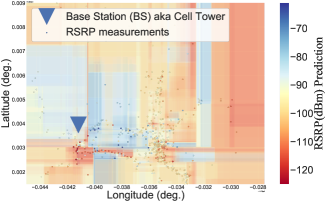
Figure 3. Example of decision boundaries chosen by RFs_x,y for Campus cell x306. We can see that RFs  can naturally identify spatially correlated measurements, i.e., regions with similar wireless propagation characteristics. For example, note how the model identifies the antenna’s backlobe and directionality.

In (Alimpertis et al., 2019), we introduced this predictor for the first time for signal maps, and we showed its superiority compared to state-of-the-art including model-based, spatiotemporal and DNN predictors. Section 4.3, including Table 6, shows that RFs outperforms alternatives on the Campus dataset. Due to lack of space, we defer the detailed evaluation of the RFs  to Appendix 52 and (Alimpertis et al., 2019; Alimpertis, 2020). In this paper, we use RFs  as the underlying ML model for our framework. However, we emphasize that the ideas of our framework build on top and can be combined with any other learning strategy that can be applied on square-integrable real functions.

RFs predictor: Under the base problem, $P_{B}$, signal map value $y\in\mathbb{Y}$ to be estimated can be modeled as follows, given a set of feature vectors $\mathbf{x}\in\mathbb{X}$. $y|\mathbf{x}\sim\mathcal{N}(RFs_{\mu}(\mathbf{x}),\sigma^{2}_{\mathbf{x}})$, where $RFs_{\mu}(\mathbf{x})$, $RFs_{\sigma}(\mathbf{x})$ are the mean and standard deviation respectively of the RFs predictor ($\equiv\widehat{f}_{y}(\mathbf{x})$). The total variance of the prediction is $\sigma^{2}_{\mathbf{x}}=RFs_{\sigma}(\mathbf{x})+\sigma^{2}_{RFs}$, where $\sigma^{2}_{RFs}$ is the error from the construction of the RFs  itself. The final prediction $\widehat{y}=\widehat{f}_{y}(\mathbf{x})=RFs_{\mu}(\mathbf{x})$ is the maximum likelihood estimate.

3.3. Quality of Service Functions ($Q(y)$)

As described above, QoS function, $Q$, is a function of KPI $y$ that reflects an outcome that depends on $y$. Examples of QoS of interest to cellular operators include the following.

Call Drop Probability (CDP). One of the most important cellular network quality metrics is the call drop probability. We model CDP with the exponential function, $Q_{cdp}(y)=ae^{-by}+c$, with parameters $a,b,c$ estimated using empirical data from the literature (Jia et al., 2015), (Iyer et al., 2017). An example of CDP vs. KPIs (RSRP and CQI) is shown on Fig. 4. It is immediately apparent that nearly all of the variation in CDP occurs at signal strengths below $-100$ dBm, implying that signal strength errors at high dBm will have far less impact on predictions of $Q_{cdp}$ than errors of equal size at low dBm. As a continuous outcome, call drop probability estimation $\widehat{Q}_{cdp}($$y$$)$ can be treated as a ML regression problem.

LTE Signal Bars. Absolute RSRP values $y$ are translated to the widely used signal bars $Q_{B}(y)$ on mobiles’ screens. Mobile analytics companies usually produce 5-colors map to visualize signal bars (Open Signal Inc., 2011). Despite variation across devices, typical values of $Q_{B}(y)$ for iOS and Android devices are:

(1) $$Q_{B}(y)=\begin{cases}0&\text{if $y^{P}<=-124$ dBm}\\ 1&\text{if $y^{P}\in[-123,-115])$ dBm}\\ 2&\text{if $y^{P}\in[-114,-105])$ dBm}\\ 3&\text{if $y^{P}\in[-104,-85])$ dBm}\\ 4&\text{otherwise ({\em i.e., }excellent reception)}\end{cases}$$

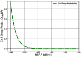
(a) $Q_{cdp}($$y^{P}$$)$ vs.  RSRP.

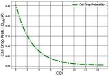
(b) $Q_{cdp}($$y^{C}$$)$ vs.  CQI.

Figure 4. Call Drop Probability (CDP) $\widehat{Q}($$y$$)$ as a function of KPIs.

Mobile Coverage. Detecting areas with weak/no signal (i.e., bad coverage) is a major problem for cellular operators. This is essentially a binary classification (per (Galindo-Serrano et al., 2013)). We define the mobile coverage indicator as a function of RSRP for LTE (Galindo-Serrano et al., 2013):

(2) $$Q_{c}(y)=\begin{cases}0&\text{if $\text{$y^{P}$}<=-115$ dBm, {\em i.e., }0 or 1 bar}\\ 1&\text{otherwise}\end{cases}$$

The rationale is that the call drop probability increases exponentially and the service deteriorates significantly below $-115$dBm (Jia et al., 2015). We want to detect areas of bad coverage because undetected $Q_{c}(y)=0$ could impact the operator’s reputation, revenue and overall performance.

Minimizing the error that matters, not MSE. We show that prediction can be improved by training models directly on QoS observations ${Q}($$y$$)$ and predicting $\widehat{Q}($$y$$)$ instead of using the proxy ${Q}($$\widehat{y}$$)$; in other words, we minimize the error of ${f_{Q}}(\mathbf{x})$ instead of minimizing the error of ${f}_{y}(\mathbf{x})$. This is equivalent to transforming the prediction problem from $P_{B}$ to some alternative $P$; intuitively, we are implicitly modifying the loss function used in estimation from one that treats errors at all $y$ values equally to one that emphasizes errors with practical consequences for cellular operators such as mis-identifying bad coverage areas or failing to predict areas with high call drop probability (e.g., see Fig. 4, $y^{P}$$<=-100$dBm). Our experimental results in Section 4 show how the prediction of bad coverage ($Q_{c}(y)=0$) can be improved for these regions that matter the most.

Prediction of $\widehat{Q}$ using Random Forests. We use RFs  to predict $\widehat{Q}$, similarly to predicting $\widehat{y}$ in the previous section. Given prediction problem $P=(Q,k)$, $Q(y)|\mathbf{x}\sim\mathcal{N}(RFs^{\prime}_{\mu}(\mathbf{x}),\sigma^{2}_{\mathbf{x}})$, where $RFs^{\prime}_{\mu}$ is trained on quality-transformed observations $(\mathbf{x}_{i},Q(y_{i}))$ instead of raw signal strength observations $(\mathbf{x}_{i},y_{i})$. This simple procedural modification (using $\widehat{Q}(y)$ in place of $Q(\hat{y}(\mathbf{x}))$) allows us to transform the base problem to any element of $P$ involving constant weight function; this last restriction is lifted below.

3.4. Importance Sampling (Weights $W$)

We have argued above that not all values of $y$ are equally important from a QoS perspective. Similarly, not all inputs $\mathbf{x}$ are necessarily equally important. For instance, an operator may be particularly interested in accurate predictions in some times or locations, e.g., 911 locations, health facilities, areas with high revenue or competitive advantage during business hours, areas with dense user population etc. We generally refer to points in the input space generically as “locations”; however the dimensions involved may include space, time, frequency, device, etc.

Prior work (Chakraborty et al., [n.d.]; Enami et al., 2018) has primarily minimized MSE for predicted signal strength via cross-validation (CV), i.e., report the error on held-out test data, after training on a sample of signal strength measurements. This implicitly assumes that all observations are equally important for both learning and evaluation, and, further, that the importance of error minimization in some subset of $\mathbb{X}$ is proportional to the number of observations in it. These are strong assumptions that are often violated in practice. For example, an operator might consider all locations within an areal unit having equal importance. If, however, the available data is distributed according to population (which is highly uneven), then the weighting implicitly used in the analysis will be far from the desired (uniform) distribution. By turns, an operator interested in population-weighted error may encounter problems when using data intensively collected by a small subset of users with residential locations or commuting patterns that are not reflective of the customer base. Such mismatches between the sampling distribution of signal strength observations in $\mathbb{X}$ and the target distribution that captures the operator’s desired loss function can be viewed as mismatches of the desired prediction problem $P(Q,W)$ versus the base problem $P_{B}$; to remove prediction bias, we show how direct estimation of $P=(Q,W)$ can be performed using techniques from importance sampling.

Table 4. Importance sampling for operators(examples)

Target Distribution (Cellular Operator Objective)	Importance Ratio (Weights $w_{i}$)
Uniform distribution $u(\mathbf{x})$	$w_{u}\propto\frac{1}{s(\mathbf{x})}$
Population distribution $d(\mathbf{x})$	$\text{$w_{d}$}\propto\frac{\text{$d(\mathbf{x})$}}{s(\mathbf{x})}$
Operator’s custom target distr. $p(\mathbf{x})$	$w_{c}\propto\frac{p(\mathbf{x})}{s(\mathbf{x})}$

3.4.1. Importance-Reweighted Prediction Error

We are interested in assessing performance via error metric corresponding to an operator-defined objective, which is some measure of expected prediction error (i) integrated over the feature space $\mathbb{X}$, (ii) with some weight function that expresses how much the operator cares about different points in that space. Consider the modified prediction problem $P=(I,W)$ (where, for now, we leave $Q=I$). The expected prediction error over the target data distribution of interest $p(\mathbf{x})$ can for this problem be written as:

(3) $$\varepsilon_{p}=\varepsilon\left(\mathbf{x},W,\widehat{y},y\right) =\int_{\mathbb{X}}W(\mathbf{x})\mathbb{E}\left[L\left(\widehat{f}(\mathbf{x})-f(\mathbf{x})\right)\right]d\mathbf{x}$$

where, $W(\mathbf{x})\rightarrow\mathbb{R}^{+}$ is the weighting function for importance sampling, $L$ is the loss function, $f(\mathbf{x})=y\rightarrow\mathbb{R}^{y}$ and $\int_{\mathbb{X}}W\left(\mathbf{x}\right)d\mathbf{x}<\infty$. If we knew $\mathbb{E}\left[L((\widehat{f}(\mathbf{x})-f(\mathbf{x})))\right]$, we could directly evaluate this integral, however we do not. We can sample from $\mathbf{x}$ and compare our predictions to true values under e.g., cross-validation (CV). However, the mean CV error itself will not in general give us $\varepsilon_{p}$, because CV is based on the sampling distribution of the data $s(\mathbf{x})$, which may look nothing like $W(\mathbf{x}),\mathbf{x}\sim p(\mathbf{x})$ (which we can interpret as target distribution, though it may not be normalized). In order to deal with the mismatch of the sampling and the target distributions, we use importance sampling techniques.

(4) $$\widehat{\varepsilon_{p}}=\frac{1}{N}\sum^{N}_{i=1}\dfrac{W\left(\mathbf{x}_{i}\right)}{s\left(\mathbf{x}_{i}\right)}\left(\widehat{f}\left(\mathbf{x}_{i}\right)-f\left(\mathbf{x}_{i}\right)\right)^{2},\mathbf{x}_{i}\sim s(\mathbf{x}_{i})$$

where $N$ is the number of sampled data points, $s\left(\mathbf{x}_{i}\right)$ is the sampling distribution, $p\left(\mathbf{x}_{i}\right)$ is the target distribution and the adjustment factor $W(\mathbf{x}_{i})/s(\mathbf{x}_{i})$ is the importance ratio. Thus, we are able to estimate an error weighted by $W(\mathbf{x})$, $\mathbf{x}\sim p(\mathbf{x})$, with data generated from the distribution $s(\mathbf{x})$. This procedure allows us to transform any method for solving $P_{B}$ into a method for solving $P=(I,W)$. The base problem weighting function is inappropriate for many practical tasks. Some intuitive examples of alternative choices of $W$ are summarized in Table 4 and described next.

(1) $\varepsilon_{u}$ uniform over $\mathbb{X}$. This is equivalent to the expected loss evaluated at a random location in $\mathbb{X}$, reflecting that the operator is equally concerned with performance over all portions of the target area. To obtain this objective function, we need $W(\mathbf{x})$ proportional to a constant, i.e., the uniform distribution $u(\mathbf{x}_{i})$. This leads to an importance ratio $w_{u}\sim\frac{1}{s(\mathbf{x})}$: we weigh each data point inversely by how often its region of the space is sampled, i.e., the inverse of the weights implicitly used by naive estimation.

(2) $\varepsilon_{d}$ proportional to population density. An intuitive target for operators is loss averaged over the user population, denoted by $d(\mathbf{x})$ at point $\mathbf{x}$ of the input space. We then want $W(\mathbf{x})\sim\text{$d(\mathbf{x})$}$, thus importance ratio $\text{$w_{d}$}\sim\frac{\text{$d(\mathbf{x})$}}{s(\mathbf{x})}$. This means that observations from parts of the user population that are rarely sampled need to be given more weight and those that are oversampled should be given less weight. It should be noted that if our sample is representative of our user population, then the naive error estimator is already an approximation of the target. However, if some groups of users are under or oversampled then the naive estimator may not perform well. Crowdsourced data collection is inherently biased due to human mobility and usage patterns.

Estimating the sampling distribution $s(\mathbf{x})$. Our observed signal strength data may have come from a known or unknown sampling design $s(\mathbf{x})$, in which case $s$ must generally be inferred. In the experimental results Section 4 we estimate $s(\mathbf{x})$ via adaptive bandwidth kernel density estimation (KDE) (Lichman and Smyth, 2014) on the 2D spatial space and the importance ratio is $w_{u}\propto\frac{u(\mathbf{l})}{s(\mathbf{l})}$. Our experimental results show that the main source of bias is location of devices.

Training Weighted Random Forests.The RFs algorithm splits each node utilizing a random set of features. The criterion of each split is to maximize the Information Gain (for classification), or to minimize the MSE (for regression). For $N$ training samples, weighted RFs (Chen et al., 2004) adjust MSE for each split according to the samples weight vector $\mathbf{w}=\left(w_{1},\cdots,w_{N}\right)$, (i.e., implicitly turning loss function to a $wMSE$) while the default setting would be $w_{i}=1$.

3.5. Shapley Values of Cellular Measurements

The Shapley Value  (Shapley, 1953) is a celebrated framework in cooperative game theory, used to assign value to the contributions of individual players. Recently, it has inspired data Shapley (Ghorbani and Zou, 2019), which quantifies the contribution of training data points in supervised machine learning. More precisely, data Shapley provides a measure of the value $\phi_{i}$ of each training data point (a.k.a. datum) $(\text{$\mathbf{x}$}_{i},y_{i})$, for a supervised ML setting which consist of: (i) a training data set $\mathcal{D}_{train}=\{(\text{$\mathbf{x}$}_{i},y_{i})\}^{N}_{1}$ , (ii) a learning algorithm $\mathcal{A}$ that produces a predictor $\widehat{y}=\widehat{f}_{y}(\mathbf{x})$ or $\widehat{f}_{Q}(\mathbf{x})$ and (iii) a performance metric $V(\mathcal{D},\mathcal{A})$. The prediction of the ML algorithm, and thus the value of the training data depend on all three. More precisely, the goal is to compute the data Shapley value $\phi_{i}(\mathcal{D},\mathcal{A},V)\equiv\phi_{i}(V)=\phi_{i}\in\mathbb{R}~{}\forall i,(\text{$\mathbf{x}$}_{i},y_{i})\in\mathcal{D}_{train}$, which follows the equitable valuation properties (i.e., null property, symmetry, summation and linearity); see Appendix A1 and  (Ghorbani and Zou, 2019) for details.

Intuition and Computation. Intuitively, a data point interacts and influences the training procedure, in conjunction with the other training points. Thus, conditions which formulate the interactions among the data points and an holistic data valuation should be considered. A simple method is leave-one-out, which calculates the datum value by leaving it out and calculating the performance score, i.e., $\phi_{i}^{\text{LOO}}=V(D)-V(D-\{i\})$. However, this formulation does not consider all subsets the point may belong to, thus does not satisfy the equitable conditions (Ghorbani and Zou, 2019). According to (Ghorbani and Zou, 2019), the data Shapley value must have the following form:

(5) $$\phi_{i}=C\sum_{\mathcal{D}-\{i\}}\frac{V(\mathcal{D}\cup\{i\})-V(\mathcal{D})}{\binom{n-1}{|\mathcal{D}|}}$$

In other words, the data Shapley value is the average of the leave-one-out value (a.k.a. marginal contributions) of all possible training subsets of data in $D_{train}$. Data Shapley, in its closed form in Eq. (6), would require an exponential number of calculations. An approximation - truncated Monte Carlo algorithm (TMC-Shapley) is provided by (Ghorbani and Zou, 2019). We adapt and extend the library for our custom error metrics, in order to estimate the data Shapley value $\phi_{i}$ of each training data point $(\text{$\mathbf{x}$}_{i},y_{i})$. More specifically, we augment it with the recall $R_{0}$ performance metric for classification, RFs regression and our reweighted-spatial uniform error $\varepsilon_{u}$ for the performance metric $V$, as defined in Sec. 3.4.

Application to Cellular Measurements and Prediction. In (Ghorbani and Zou, 2019), the Data Shapley value was tacitly defined for classification of medical data. In this paper, we apply, for the first time, Data Shapley valuation to mobile performance data, and not only for the base problem $P_{B}$ but also for the general problem $P=(Q,W)$. The input to data Shapley in our context is: (i) the available cellular measurement data used for training (ii) the ML prediction algorithm (RFs) and (ii) the performance metric $V$, which in our case we define as the re-weighted error based on the operators’ objectives, presented earlier in the paper. The output is a value assigned to each individual measurement training data point, used for the training for the particular prediction task $(Q,W)$.

Data Shapley vs. Weight Functions: We have already described earlier how both the choice of a loss function and of the evaluation metric really matter (Sec. 3.3 and 3.4.1). Data Shapley and weight functions share common characteristics but they also have differences, and can complement each other creating a powerful framework. Each framework independently can inform us whether the data are scarce and valuable for our objective, hence can inform how to acquire future data to improve the predictor. However, weight functions on their own do not not quantify the contribution of training data points, e.g., if a training data point is an outlier. On the other hand, data Shapley inherently requires a performance score to evaluate the test data. There is no universal data valuation and for different learning tasks (i.e., objectives) some data points might be more valuable than other. Our $(Q,W)$ framework thus define the reweighted error, which provides the performance score for the data Shapley value.

Using data Shapley and preview of results. Having computed the Shapley values of our cellular measurement data, we can then use them to remove measurements with negative or low Shapley values, in order to both (i) improve prediction and (ii) achieve data minimization. The results in Sec. 4.7 show that we can remove up to 65-70% of data, while improving the recall for coverage from 64% to 99%.

Table 5. Overview of datasets used throughout the paper. Campus is collected by us on our university campus. NYC and LA were provided by a Mobile Analytics Company

Dataset	Period	Areas	Type of Measurements	Characteristics
Campus	02/10/17 - 06/18/17	Univ. Campus Area $\approxeq 3km^{2}$	LTE KPIs: RSRP, [RSRQ]. Context: GPS Location, timestamp, $dev$, $cid$. Features: $\mathbf{x}=\left(l_{j}^{x},l_{j}^{y},d,h,dev,out,||\vec{l}_{\text{BS}}-\vec{l}_{j}||_{2}\right)$	No. Cells $=25$ No. Meas $\approxeq 180$K Density ($\frac{N}{m^{2}}$) Per Cell: $0.01$ - $0.66$ (Table 3) Overall Density: $0.06$
NYC & LA	09/01/17- 11/30/17	NYC Metropolitan Area $\approxeq 300km^{2}$	LTE KPIs: RSRP, RSRQ, CQI. Context: GPS Location, timestamp, $dev$, $cid$. EARFCN. Features:$\mathbf{x}=\left(l_{j}^{x},l_{j}^{y},d,h,cid,dev,out,||\vec{l}_{\text{BS}}-\vec{l}_{j}||_{2},freq_{dl}\right)$	No. Meas NYC $\approxeq 4.2$M No. Cells NYC $\approxeq 88k$ Density NYC-all $\approxeq 0.014\frac{N}{m^{2}}$
		LA metropolitan Area $\approxeq 1600km^{2}$		No. Meas LA $\approxeq 6.7$M No. Cells LA $\approxeq 111$K Density LA-all $\approxeq 0.0042\frac{N}{m^{2}}$

4. Performance Evaluation

4.1. Data Sets

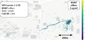
(a) Campus example cell x204: high density ($0.66$), low dispersion (325).

(b) Campus: example cell x355: small density ($0.12$) more dispersed data ($573$).

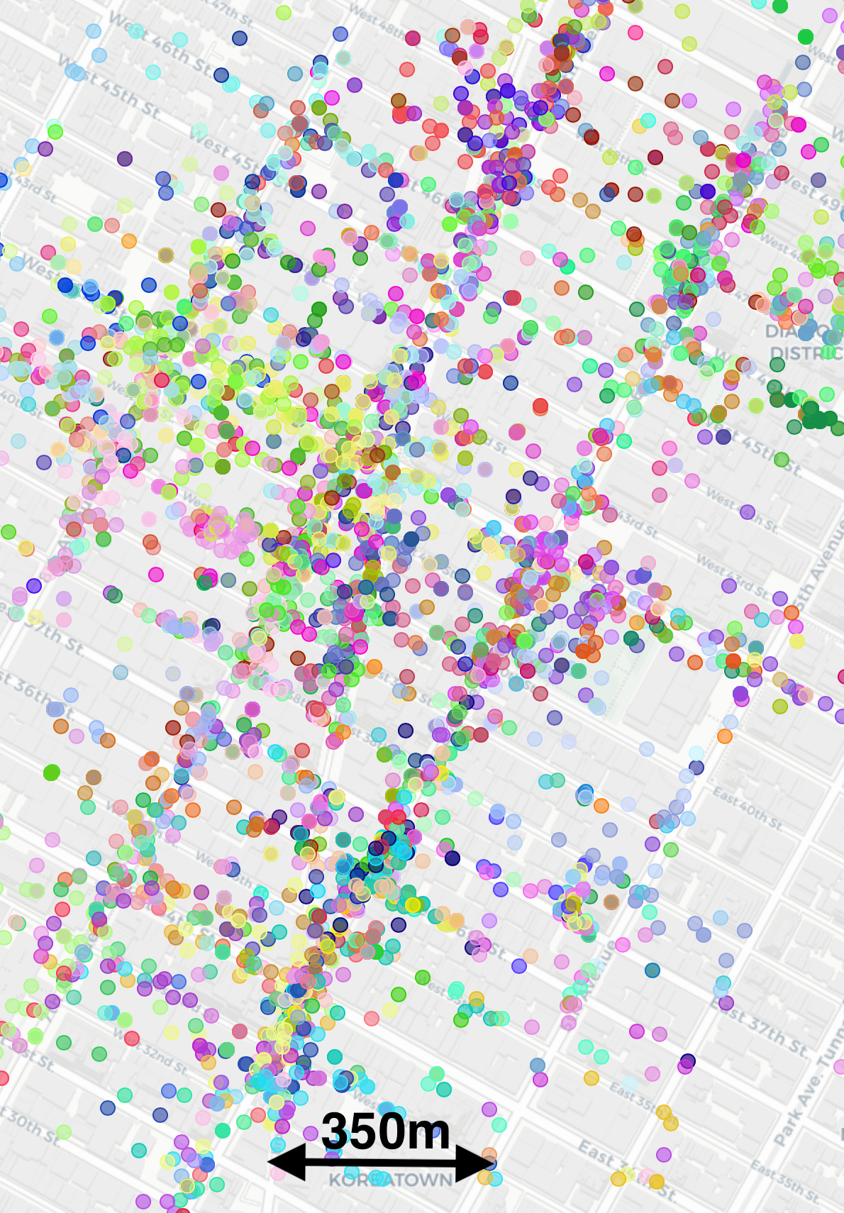
(c) NYC: Manhattan LTE TA

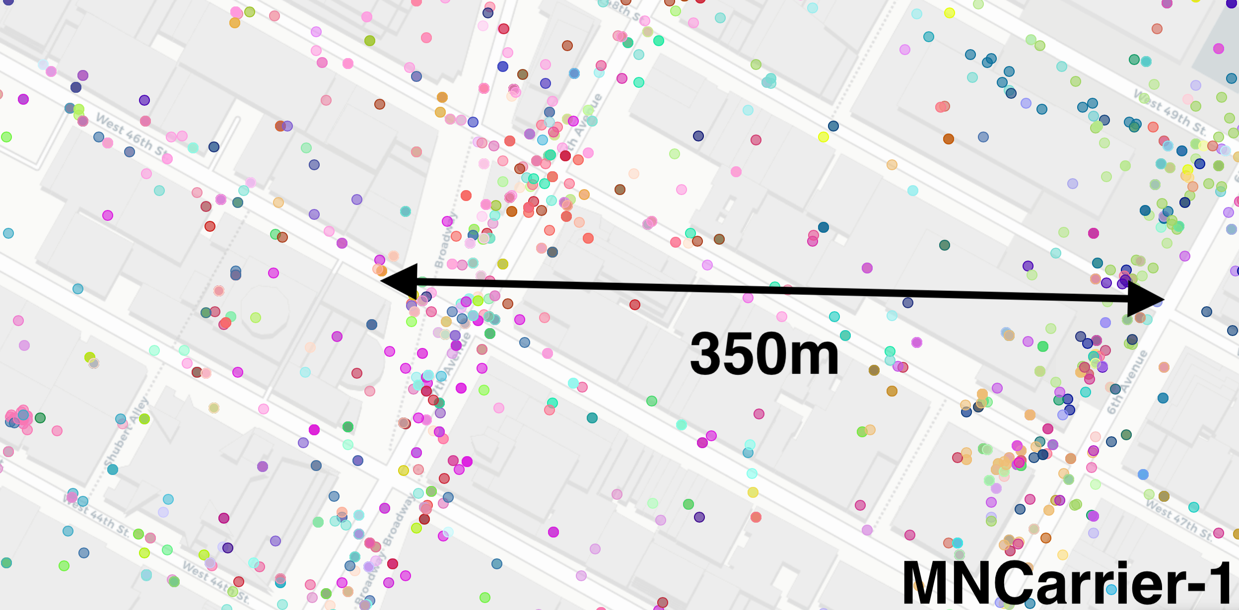
(d) NYC: zooming in Manhattan Midtown (Time Square) for some of the available cells.

Figure 5. LTE RSRP Map Examples from our datasets. (a)-(b): Campus dataset. Color indicates RSRP value. (c)-(d): NYC dataset. Data for a group of LTE cells in the Manhattan Midtown area. Different colors indicate different cell IDs.

We evaluate our framework using two types of real-world LTE datasets obtained in prior work (Alimpertis et al., 2019), the characteristics of which are summarized on Table 5. Both datasets include cellular measurements, and we use the same subset of information from all datasets, e.g., RSRP, RSRQ or CQI values and the corresponding features defined in Section 3. User identifiers were neither collected nor stored for this study.

Data Format. We use the same subset of information from all datasets, e.g., RSRP, RSRQ or CQI values and the corresponding features defined in Section 3. An example, in GeoJSON, with some of the KPIs fields (obfuscated) is shown below:

⬇ {”type”: ”Feature”, ”properties”: { ”timestamp”: ”2017-09-11T17:54:35EDT”, ”lteMeasurement”: {”rsrp”: -89, ”rsrq”: -20, ”cqi”: 9, ”pci”: 169, ”earfcn”: 9820}, ”cell”: { ”ci”: xxxxx710, ”mnc”: 410, ”mcc”: 310, ”tac”: xx22, ”networkType”: 4}, ”device” : {”manufacturer”:”samsung”, ”model”:”SM-G935P”, ”os”:”android70”}, ”locationMetaData”: {”city”: ”New␣York”, ”accuracy”: ”x”,”velocity”:”x”}}, ”geometry”: {”type”: ”Point”,”coords”: [-73.9x,40.7x]}}\end{lstlisting} %\vspace{-10pt} \end{mdframed} %\vspace{-10pt} Listing 1: GeoJSON example with LTE KPIs and location, in MongoDB (obfuscated for presentation). Campus Dataset. We collected the first dataset on our university campus, via a user-space Android app we developed ourselves and used to collect data from volunteers  (Alimpertis and Markopoulou, 2017). This Campus dataset is relatively small: $180,000$ data points, collected by seven Android devices that belong to graduate students, using 2 cellular providers, and moving between student housing, offices and other locations on campus (approx. $3km^{2}$). However, this is a dense dataset, with multiple measurements over time on nearby locations. Due to space limitations, we refer to  (Alimpertis and Markopoulou, 2017; Alimpertis et al., 2019) for details. NYC and LA datasets. These were collected by a major mobile crowdsourcing and data analytics company and shared with us (after appropriate anonymization). They contain $10.9$M measurements, covering approx. $300km^{2}$ and $1600km^{2}$ in the metropolitan areas of NYC and LA, respectively, for a period of 3 months with tens of thousands of unique cells (i.e., unique $cID$). An example of the NYC neighborhood in East NYC is depicted in Fig. 2. Examples of representative LTE TAs from NYC and LA datasets used in our evaluation are summarized later in Table 10. These are large datasets in terms of any metric, such as number of measurements, geographical scale, number of cells etc. As such, they provide novel insight into the problem at a scale that is relevant to operators and mobile analytics companies.

4.2. Evaluation Setup

RFs predictor. We train Random Forest (RFs) to predict the KPI $\widehat{y}$; then we compute ${Q}($$\widehat{y}$$)$) or $\widehat{Q}(y)$ directly. We use state-of-the-art RFs (Alimpertis et al., 2019) as the underlying predictor, but it could be replaced by other ML models. The most important hyper-parameters for RFs are the number of decision trees (i.e., $n_{trees}$) and the maximum depth of each tree (i.e., $\text{max}_{depth}$). We used a grid search over the parameter values of the RFs  estimator (Pedregosa et al., 2011) in a small hold-out part of the data to select the best values. For the Campus dataset, we select $n_{trees}=20$ and $\text{max}_{depth}=20$ via 5-Fold CV; larger $\text{max}_{depth}$ values could result in overfitting of RFs. For the NYC and LA datasets, we select $n_{trees}=1000$ and $\text{max}_{depth}=30$; more and deeper trees are required for larger datasets. An important design choice is the granularity we choose to build our RFs models. As we demonstrated in (Alimpertis et al., 2019), using a model per cell (i.e., train a separate RFs  model per cell $cID$  with $\mathbf{x_{j}^{-cID}}=\{x:x\in\mathbf{x_{j}^{full}},\sim x\notin\{cID\}\}$) is beneficial for large number of measurements per $cID$. In sparser data, such as NYC and LA datasets, it is better to train a model per LTE TA  using $\mathbf{x_{j}^{full}}$. In this paper, we utilize models per $cID$ for the Campus dataset and per LTE TA models for NYC and LA datasets as (Alimpertis et al., 2019). To improve the reweighted prediction error $\varepsilon_{p}$ according to operators’  objectives (Section 3.4), we train weighted random forests RFs_w, with $w_{i}=\{w_{u_{i}},w_{d_{i}}\}$ proportionally to the target distribution (see Table 4). In essence, the ML training weights are set equal to the importance ratio of each sample (Katharopoulos and Fleuret, 2018). We compare RFs_w with the default RFs, where all samples are weighted equally. Data Shapley Setup. For $\widehat{\phi_{i}}$ estimation with the TMC-Shap algorithm, work in (Ghorbani and Zou, 2019) suggests a convergence (stopping) criterion of $\frac{1}{n}\sum_{i=1}^{n}\frac{|\phi_{i}^{t}-\phi_{i}^{t-100}|}{|\phi_{i}^{t}|}<0.05$ with an observation that the algorithm usually convergences with up to $3N_{train}$ iterations. However, our datasets are significantly larger; (Ghorbani and Zou, 2019) use approx. up to $3000$ points and on the contrary the cell x$901$ demonstrated later contains approx. $15000$ measurements. Thus, we relax the convergence criterion to save execution time and we set a 30% convergence if we exceed 2$N_{train}$ iterations. Splitting Training vs. Testing. We select randomly $70\%$ of the data as the training set $\mathcal{D}_{train}=\{\mathbf{X}_{train},\mathbf{y}_{train}\}$ and $30\%$ of the data as the  testing  set $\mathcal{D}_{test}=\{\mathbf{X}_{test},\mathbf{y}_{test}\}$ for the problem of predicting missing signal map values (i.e., KPIs $y=\{\text{$y^{P}$, $y^{I}$, $y^{C}$}\}$ or QoS $Q_{c}(y)$, $Q_{cdp}($y$)$). The reported results are averaged over $S=10$ random splits. Our choices differ for data Shapley where we split the data as following: 60% of the data for $\mathcal{D}_{train}=\{\mathbf{X}_{train},\mathbf{y}_{train}\}$, 20% for $\mathcal{D}_{test}=\{\mathbf{X}_{test},\mathbf{y}_{test}\}$ and 20% for the held-out set $\mathcal{D}_{\text{held-out}}$. Data Shapley values $\phi_{i}$ are being calculated per training point $(\text{$\mathbf{x}$}_{i},y_{i})$ w.r.t. the performance score $V$ of the prediction on $\mathcal{D}_{test}$. We use the $\mathcal{D}_{\text{held-out}}$ dataset to report the final data minimization results, i.e., use some completely unseen data since $\mathcal{D}_{test}$ was used for the data Shapley $\phi_{i}$ itself. Evaluation Metrics - Coverage Classification. We evaluate the performance of $Q_{c}(y)$ in terms of binary classification metrics, i.e., recall, precision, F1 score and balanced accuracy. Recall is defined as $R=\frac{T_{p}}{T_{p}+F_{n}}$ where $T_{p}$ is the true positive rate and $F_{n}$ is the false negative rate, for the class of interest. Precision is defined as $Pr=\frac{T_{p}}{T_{p}+F_{p}}$. F1 Score is the weighted average of precision and recall and Balanced Accuracy the average of recall for each class. Evaluation Metrics for Regression. (I) Root MSE ($RMSE$). If $\widehat{y}$ is an estimator for $y$, then $RMSE(\widehat{y})=\sqrt{MSE(\widehat{y})}=\sqrt{E((y-\widehat{y})^{2})}$, in dB for RSRP $y^{P}$and RSRQ $y^{I}$and unitless for CQI $y^{C}$. (II) Reweighted Error $\varepsilon_{p}$ for a target distribution $p(\mathbf{x})$. According to Eq. (4), $\varepsilon_{p}=\frac{1}{N}\sum_{i=1}^{N}w_{i}\left(\widehat{y}_{i}-y_{i}\right)^{2}$, with $w_{i}=\{w_{u_{i}},w_{d_{i}}\}\propto\{\frac{1}{s(\mathbf{l}_{i})},\frac{\text{${d}($$\mathbf{l}_{i}$$)$}}{s(\mathbf{l}_{i})}\}$, as defined in Table 4, where $w_{u}$ corresponding to the importance ratio for error in a random location in $\mathbb{X}$ and $w_{P}$ the weighting proportional to population density. We use only location density $s(\mathbf{l})$ to calculate the (i) uniform error $\varepsilon_{u}$ or (ii) $w_{d}$, over the space $\mathbb{X}$, but our methodology is applicable to an arbitrary space $\mathbb{X}$.

4.3. Results for Base Problem $P=($$I,k$$)$

Prior work has exclusively focused on RSRP prediction minimizing MSE. Evaluating the performance of RFs  for this base problem is necessary to show that our RFs based predictor (Alimpertis et al., 2019) is a good choice for the underlying “workhorse” ML predictor on top of which, we can develop our $P=(Q,W)$ framework. We compare RFs against several baselines: model-driven (LDPL-knn and LDPL-hom), geospatial interpolation (OK and OKD), and a multilayer DNN (trained with $l^{x},l^{y}$ features). We show that RFs achieves lower MSE than all those alternatives: Table 6 shows that comparison of all predictors for the cells of the Campus dataset. Due to space constraints, and since this is not a core contribution of this paper, we defer additional evaluation details to Appendix A2 and our prior work in (Alimpertis et al., 2019). We emphasize that our framework builds on top of the base predictor, which can be swapped for other state-of-the art square loss predictors, as those become available. For the rest of the paper, we focus on evaluating our framework for $P=($Q,W$)$, which essentially modifies the loss function on the base problem $P_{B}=(I,k)$, and the data Shapley valuation ($\phi$). Table 6. Campus dataset: Comparing predictors per cell ($cID$) for the Base Problem, $P=($$I,k$$)$, for all cells of the Campus dataset. One can see that the RFs  predictor (last columns) achieves lower MSE than all alternative predictors (LDPL, OK, OKD, DNN), and is therefore a good choice. Cell Characteristics $RMSE$ (dB) $cID$ $N$ $\frac{N}{\text{sq }m^{2}}$ $\operatorname{\mathbb{E}}[P]$ $\sigma^{2}$ LDPL hom LDPL $\scriptstyle{kNN}$ OK OKD DNN $RFs$ $\scriptstyle{x,y}$ $RFs$ $\scriptstyle{x,y,t}$ $\scriptstyle{RFs}$ $\scriptscriptstyle{all}$ x312 10140 0.015 -120.6 12.0 17.5 1.63 1.70 1.37 2.05 1.58 0.93 0.92 x914 3215 0.007 -94.5 96.3 13.3 3.47 3.59 2.28 6.48 3.43 1.71 1.67 x034 1564 0.010 -101.2 337.5 19.5 7.82 7.44 5.12 11.59 7.56 3.82 3.84 x901 16051 0.162 -107.9 82.3 8.9 4.60 4.72 3.04 5.69 4.54 1.73 1.66 x204 55566 0.666 -96.0 23.9 6.9 3.84 3.85 2.99 4.44 3.83 2.30 2.27 x922 3996 0.107 -102.7 29.5 5.6 3.1 3.16 2.01 4.51 3.10 1.92 1.82 x902 34193 0.187 -111.5 8.1 21.0 2.60 2.47 1.64 2.8 2.50 1.37 1.37 x470 7699 0.034 -107.3 16.9 24.8 3.64 2.73 1.87 3.33 2.78 1.26 1.26 x915 4733 0.042 -110.6 203.9 14.3 7.54 7.39 4.25 9.94 7.31 3.29 3.15 x808 12153 0.035 -105.1 7.7 4.40 2.41 2.42 1.60 2.84 2.34 1.75 1.59 x460 4077 0.040 -88.0 32.8 11.2 2.35 2.28 1.56 3.60 2.31 1.84 1.84 x306 4076 0.011 -99.2 133.3 18.3 4.85 4.30 2.80 7.07 3.94 3.1 3.06 x355 30084 0.116 -94.3 42.6 9.3 2.42 2.31 1.85 3.28 2.26 1.79 1.79

4.4. Results for QoS functions $P=(Q,k)$

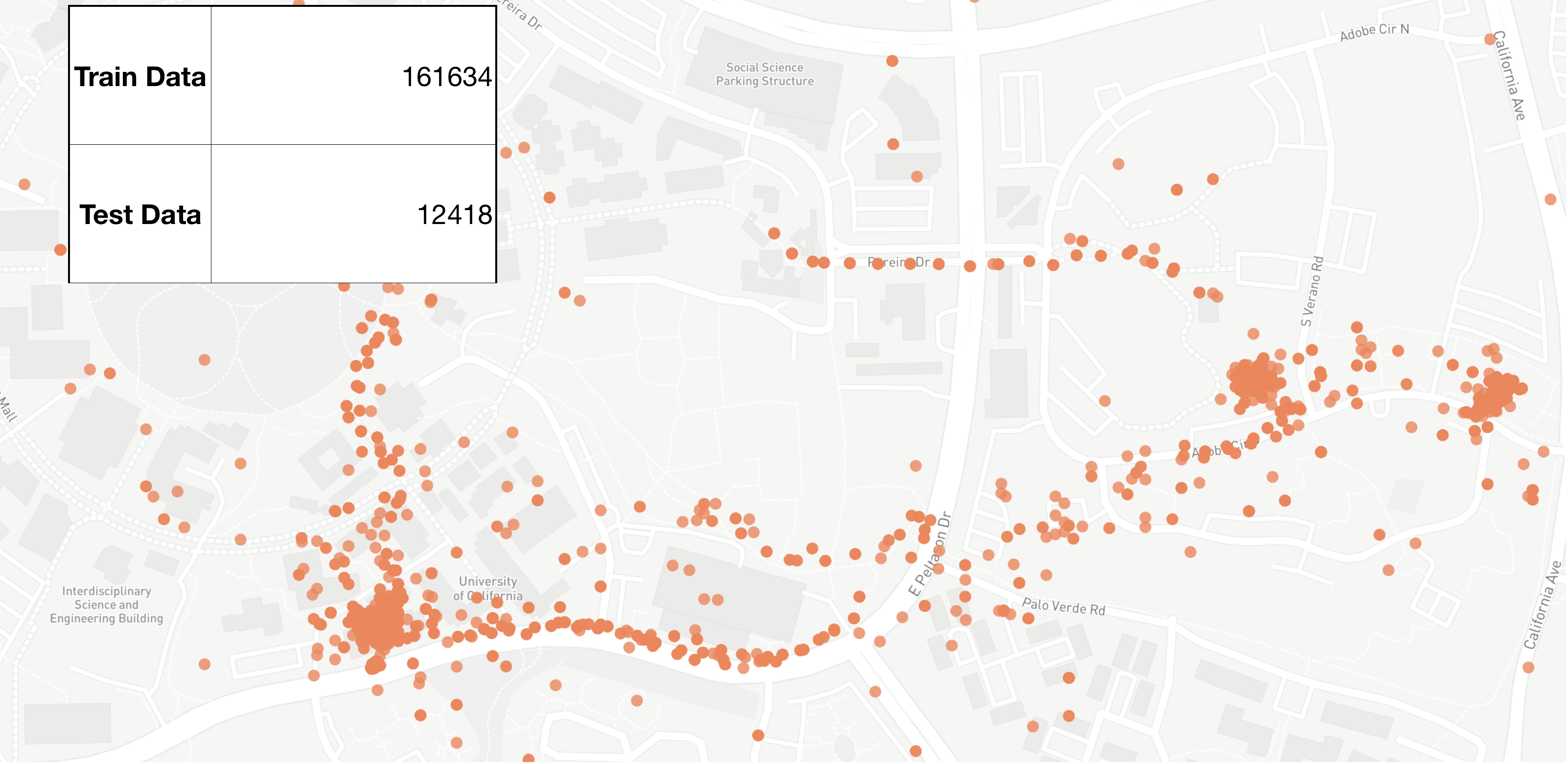
(a) Actual Spots with Bad Coverage.

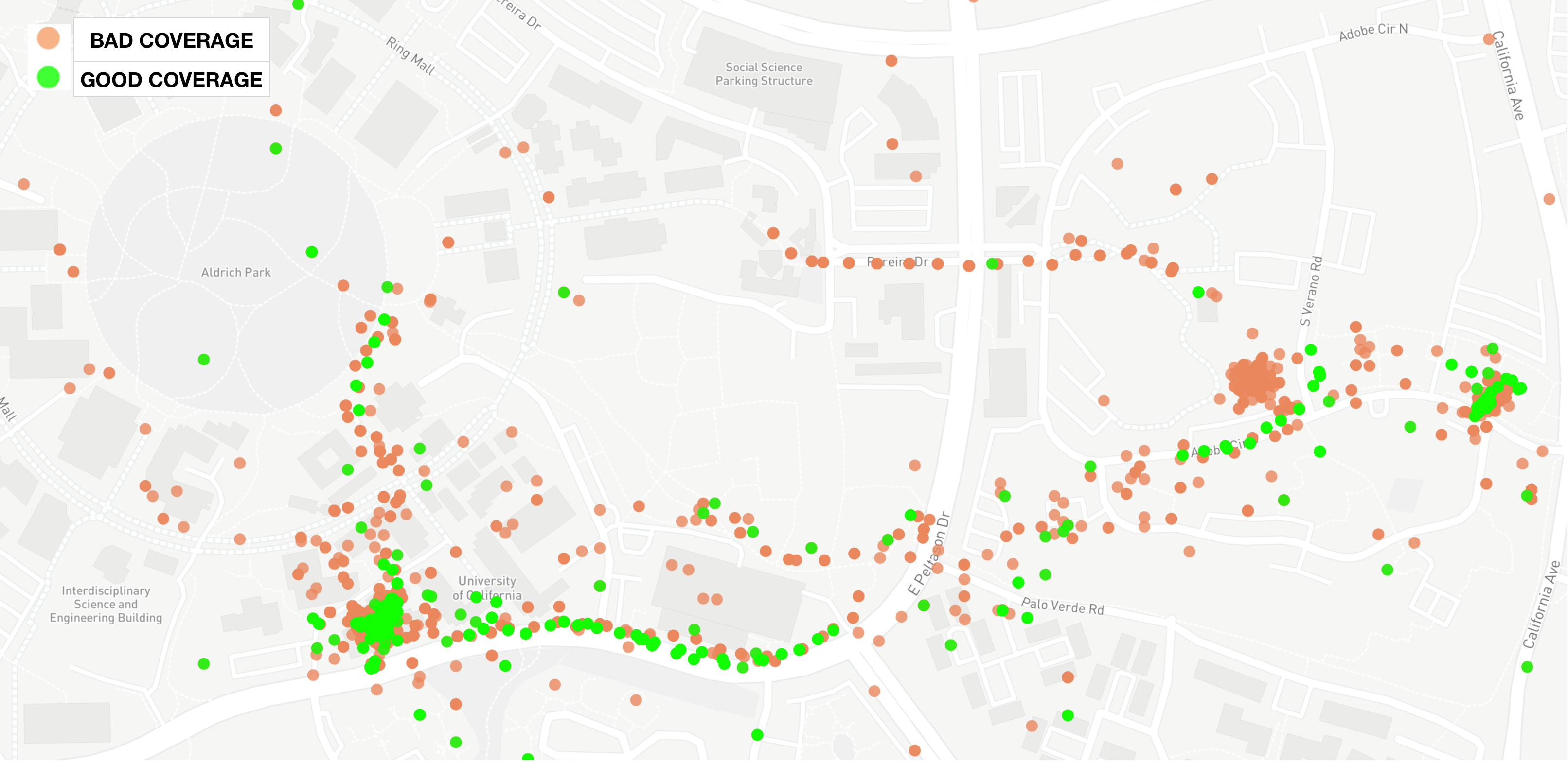
(b) Baseline Prediction ${Q}($$\widehat{y}$$)$.

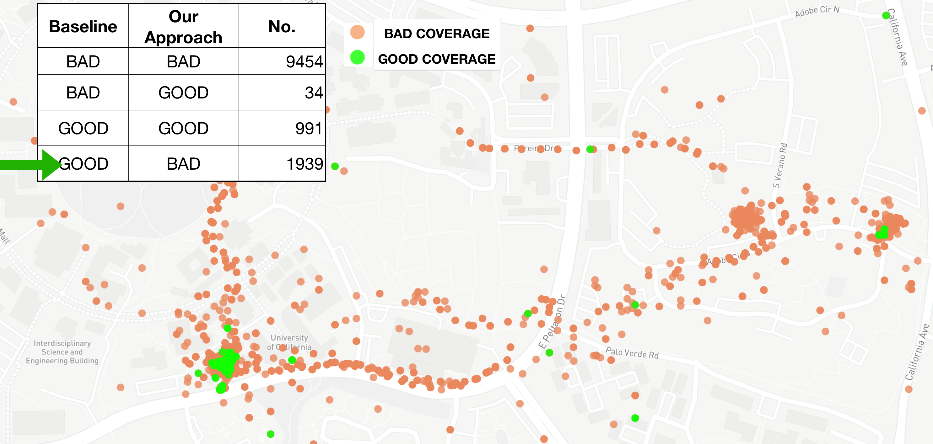
(c) Our Approach $\widehat{Q_{c}}(y)$

Figure 6. LTE Coverage Map for our own Campus dataset. Display only Test Data. (a) Bad Coverage from Test Data (b) Baseline-Proxy- Prediction ${Q}($$\widehat{y}$$)$ (c) Our Model Prediction. It can be seen that (c) has more red points than (b), implying better classification. For this example, we discover 1939 data points which the baseline would not detect (16% of the total 12418 bad coverage points). Best viewed in color.

4.4.1. Coverage Domain, $P=($$Q_{c},k$$)$

This setup is a typical binary classification problem, where class 0 corresponds to bad coverage and class 1 corresponds to good coverage. As a baseline, we train the RFs regression models, we predict $\widehat{y}$ and compute the proxy ${Q}($$\widehat{y}$$)$. We compare that with our proposed approach, which is to train RFs classifiers, with the same features, on quality-transformed observations $(\mathbf{x}_{i},Q(y_{i}))$ and predicting $\widehat{Q}(y)$. For coverage indicator, we employ $y=$$y^{P}$since it is defined on RSRP. RFs use the default training ($\forall i,w_{i}=1$). In this setup, bad coverage (class-0) misclassified as good coverage areas (class-1) impact reputation, revenue, and overall performance. Therefore, from the operators’ perspective, it is desirable to maximize the Recall for class-0 $R_{0}$ because higher Recall means fewer false negatives, i.e., our algorithm did not classify a bad coverage ($Q(y)=0$) as a good coverage area ($\hat{Q}(y)=1$).

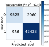
(a) Baseline-Proxy $Q_{c}(\widehat{y})$

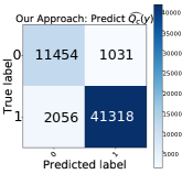
(b) Our method $\widehat{Q}_{cdp}(y)$.

Figure 7. For Campus dataset: Confusion Matrix for coverage, $Q_{c}(y)$ ($P=($$Q_{c},k$$)$). The points incorrectly classified as “good coverage” by the baseline $Q_{c}(\widehat{y})$ predictor are shifted to the “bad coverage” class under our predictor $\widehat{Q}(y)$. Recall Precision F-1 Accuracy Balanced Accuracy Class Label 0 1 0 1 0 1 $Q_{c}(\widehat{y})$ 0.762 0.978 0.910 0.934 0.830 0.956 0.930 0.870 $\widehat{Q_{c}}(y)$ 0.917 0.952 0.847 0.975 0.881 0.963 0.944 0.935 Table 7. Campus Coverage $Q_{c}(y)$ results: (i) Recall for Class-0 (No-Coverage) 76% $\rightarrow$ $92\%$, (ii) Accuracy and (iii) Balanced Accuracy Improve. The improved Recall ($R_{0}$) is of immense importance for Cellular Providers; higher $R_{0}$ means less false negatives for $Q_{c}(y)$ (i.e., miss-classifications of bad coverage to good coverage). (a) Campus dataset: Fig. 6 illustrates the improvement in the Campus dataset from utilizing our predictor $\widehat{Q}(y)$ instead of the naive proxy $Q_{c}(\widehat{y})$ for bad coverage spots. For this example, we discover 1939 bad coverage sites that the baseline did not detect (16% of the total 12418 bad coverage points). Moreover, Fig. 6(c) shows how the bad coverage spots which were mis-classified as good coverage spots have been reduced by our predictor $\widehat{Q_{c}}(y)$, especially in areas of densely sampled data and commute traces (note the road and path trajectories). The confusion matrix for these results is shown in Fig. 7, where we can see again the shift of points incorrectly classified as “good coverage” by the baseline $Q_{c}(\widehat{y})$ predictor to the “bad coverage” class under our predictor. The overall classification results, in terms of the binary classification metrics, are shown in Table 7. We see an improvement of 16% for Recall $R_{0}$, per Fig. 6, as well an improvement in balanced accuracy from 87% to 94%. These improvements do not come at the expense of F1 and Accuracy, which improve by approx. 1%. (b) NYC and LA datasets: Table 8 lists the classification results for some examples from NYC and LA datasets. We see a similar increase up to 12% in terms of $R_{0}$ for our predictor $\widehat{Q_{c}}(y)$ compared to the baseline proxy. Recall Precision F-1 Accuracy Balanced Accuracy Class Label 0 1 0 1 0 1 MNC-1, LTE-TA: x552, Eastern Brooklyn $Q_{c}(\widehat{y})$ 0.55 0.98 0.80 0.93 0.65 0.96 0.93 0.77 $\widehat{Q_{c}}(y)$ 0.67 0.95 0.70 0.95 0.68 0.96 0.93 0.81 MNC-1, LTE-TA: x641, LA, Covina - Hacienda Heights $Q_{c}(\widehat{y})$ 0.58 0.90 0.73 0.82 0.65 0.86 0.80 0.74 $\widehat{Q_{c}}(y)$ 0.70 0.86 0.70 0.86 0.70 0.86 0.81 0.78 Table 8. NYC and LA datasets Coverage $Q_{c}(y)$ results. Recall $R_{0}$ improves up to 12%. Operators would ideally minimize the false negatives of class-0. Similar results observer in other LTE TAs .

4.4.2. Call Drop Probability Domain, $P=($$Q_{cdp},k$$)$

CDP $Q_{cdp}($y$)$ estimation is a continuous value prediction problem on the [0,1] interval. As with the coverage domain, we train RFs models in order to predict $\widehat{y}$ and use the proxy $Q_{cdp}(\widehat{y})$ as a baseline. We compare that with our approach, which is to train RFs, using the same features, on quality-transformed observations $(\mathbf{x}_{i},Q(y_{i}))$ and predict $\widehat{Q_{cdp}}(y)$. We report the relative reduction in $RMSE$. (a) Campus dataset: In Fig. 8, we report results for estimating CDP, when using the proxy baseline vs. predicting CDP directly. Fig. 8(a) shows the relative reduction in $RMSE$ error of CDP estimation vs. RSRP, which confirms our design choice. Our estimation $\widehat{Q}_{cdp}(y)$ reduces the relative estimation error up to 27% in the lower reception regime (0-1 vars, $y^{P}$$\leq-115$dBm), where the error function being minimized is highly sensitive to predictive performance.

From $Q_{cdp}(y)$ to the RSRP $y^{P}=y$ domain (i.e., transform $P=(Q,k)\rightarrow P_{B}=(I,k)$):

It is important to highlight that our QoS domain methodology can also improves RSRP prediction itself for values with high CDP that matter the most. An example is shown in Fig. 8(b): we compare the prediction error of $\widehat{y}$ values (RSRP) themselves, vs. inverting $\widehat{Q}_{cdp}(y)$ to return back to the original $y^{P}$ space. We group the error by signal bars and we observe that the change in learning objective shifts the effort to reducing error where it is most critical (in lower signal strength range). We basically exploit the fact that we can tolerate higher uncertainty at high RSRP (where a large error has little impact on predicted CDP). We can hence view our procedure as allowing us to train on an application-specific loss function, without modifying our underlying learning algorithm.

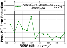
(a) $RMSE$ Relative Reduction.

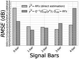
(b) $Q_{cdp}(y)\leftrightarrow$ RSRP $y$

Figure 8. Improving the RSRP prediction itself via $P=(Q,k)\rightarrow P_{B}=(I,k)$ transform, for the Campus dataset. (a) $Q_{cdp}($$y$$)$ $RMSE$ vs. RSRP. Our methodology reduces the error up to 27% for lower RSRP values (0-1 bars). (b) $Q^{-1}(\widehat{Q}_{cdp})$ $RMSE$ vs. Predicting directly RSRP values: the improvement has shifted towards the lower RSRP (fewer bars) accordingly to the new QoS function $Q_{cdp}(y)$ we trained for. (b) NYC and LA datasets: We also present results for CDP prediction on the NYC and LA datasets, and using RSRQ $y^{I}$and CQI $y^{C}$data in addition to RSRP $y^{P}$. Fig. 10(a) and Fig. 10(b) show $RMSE$ of CDP estimation with RSRQ $y^{I}$and CQI $y^{C}$respectively. The different KPIs and the use of per-$cID$ models in one case (RSRQ $y^{I}$) do not change the improvements from our technique. We improve in the low KPI $y$ regime up to 0.1 in absolute error value (in the probability domain); in terms of relative error our method $\widehat{Q}_{cdp}(y)$ performs up to 32% better than the baseline $Q_{cdp}(\widehat{y})$ for CDP estimation. For $Q_{cdp}($$y$$)$ and $Q_{c}(y)$, similar results were observed for other LTE TAs for NYC and LA datasets but omitted due to lack of space. Fig. 9 summarizes the performance of CDP estimation for the different LTE TAs (i.e., areas) available in our dataset. We plot the $\log$-ratio of the $RMSE$ of the baseline vs. our approach. Values greater than 1 indicate improvement for our model as in the other examples, we see that our procedure successfully focuses improvement where it is needed for CDP prediction, rather than wasting statistical power on the high signal strength regime.

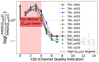
(a) CDP with CQI $y=$$y^{C}$

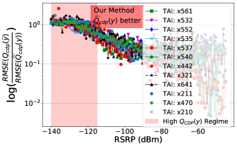
(b) CDP with RSRP $y=$$y^{I}$

Figure 9. NYC and LA datasets Call Drop Probability $Q_{cdp}($$y$$)$ estimation.

4.4.3. Discussion: why minimizing MSE can be naive.

In signal strength prediction, an error of few (say 5) dB will not reflect much change in QoS when the user’s received signal strength is high (e.g., -50 to -60 dBm, see Fig. 4). The user experiences excellent QoS in that regime, and hence even moderately large errors in predicted RSRP would not greatly impact predictions of QoS. In contrast, an error of $5$dB would substantially affect QoS prediction in the weak reception regime (e.g., for -120dBm vs.-125dBm you can notice the large difference in CDP in Fig. 4). For QoS prediction, it can hence be worth trading greater RSRP error in the high-strength regime for lower error in the low-strength regime, as we demonstrated. Working directly with ${Q}($$y$$)$ alters our application loss function so as to focus performance where it is most needed, but without requiring us to modify the RFs procedure to change its nominal loss function). The result is improved performance for QoS outcomes, here up to 32% for the values that matter more to cellular operators.

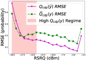
(a) NYC:Manhattan Uptown

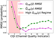
(b) LA: Suburb x470

Figure 10. Call Drop Probability $Q_{cdp}($$y$$)$ estimation for NYC and LA datasets. (a) RSRQ ($y=$ $y^{I}$), Models Per $cID$. (b) CQI ($y=$ $y^{C}$).

4.5. Results for Importance Sampling $P=(I,W)$

Next, we evaluate our framework in terms of the reweighted error $\varepsilon_{p}$. We predict RSRP and we compare a default setting RFs vs. RFs_w (i.e., $w_{i}$ are set to importance ratio as described in Section 4.2).

4.5.1. $\varepsilon_{u}$ over Uniform Spatial Distribution, $P=($$I,w_{u}$$)$.

(a) Campus dataset: To calculate the importance ratio $w_{u}=1/s(\mathbf{l})$ we estimate $s(\mathbf{l})$ with adaptive bandwidth KDE over the spatial dimensions as we describe in 3.4. Table 9 reports the error $\varepsilon_{u}$ for both the default RFs predictor and the RFs_w. We observe an improvement of up to 20% for $\varepsilon_{u}$ for cells that are oversampled in just few locations; the average relative improvement is approx. 5%, which demonstrates the benefit of readjusting the training loss. Cell Characteristics Default $RFs$ $\rightarrow\widehat{y}$ $RFs_{w_{u}}$ $\rightarrow\widehat{y}_{w}$ Improvement $cID$ $N$ $\sqrt{\varepsilon_{u}}$ $\sqrt{\varepsilon_{u}}$ Diff. Diff. (%) x922 3955 0.86 0.69 0.17 19.6 x808 12153 1.54 1.25 0.28 18.5 x470 7688 0.71 0.59 0.12 17.0 x460 4069 1.66 1.44 0.22 13.1 x355 29608 1.77 1.57 0.20 11.5 x306 4027 2.21 2.03 0.18 8.1 x901 16049 0.94 0.91 0.03 3.4 x902* 34164 1.93 1.90 0.03 1.5 x914 3041 1.66 1.64 0.02 1.0 x915 4725 1.81 1.80 0.00 0.2 x312 9727 0.64 0.65 -0.01 -0.6 x204* 55413 0.91 0.94 -0.03 -3.2 x034 1554 2.43 2.68 -0.24 -10.0 All 186173 1.34 1.28 0.06 4.89 Table 9. Campus dataset,  RSRP $y$ prediction: $\varepsilon_{u}$ Error (i.e., reweighted according to the uniform distribution $\equiv$ $P=($$I,w_{u}$$)$): (i) Train on Default RFs vs.  (ii) train on RFs_w $w_{i}=w_{u}\propto\frac{1}{s(\mathbf{l})}$. Models per $cID$. For each $cID$ and training case, we pick the best performing adaptive bandwidth KDE for estimating $s(\mathbf{l})$. Our methodology shows improvement up to approx. $20\%$. For cells * with extremely high sampling density in few locations -see (Alimpertis et al., 2019)-, we utilize fixed bandwidth estimation both in space and time.

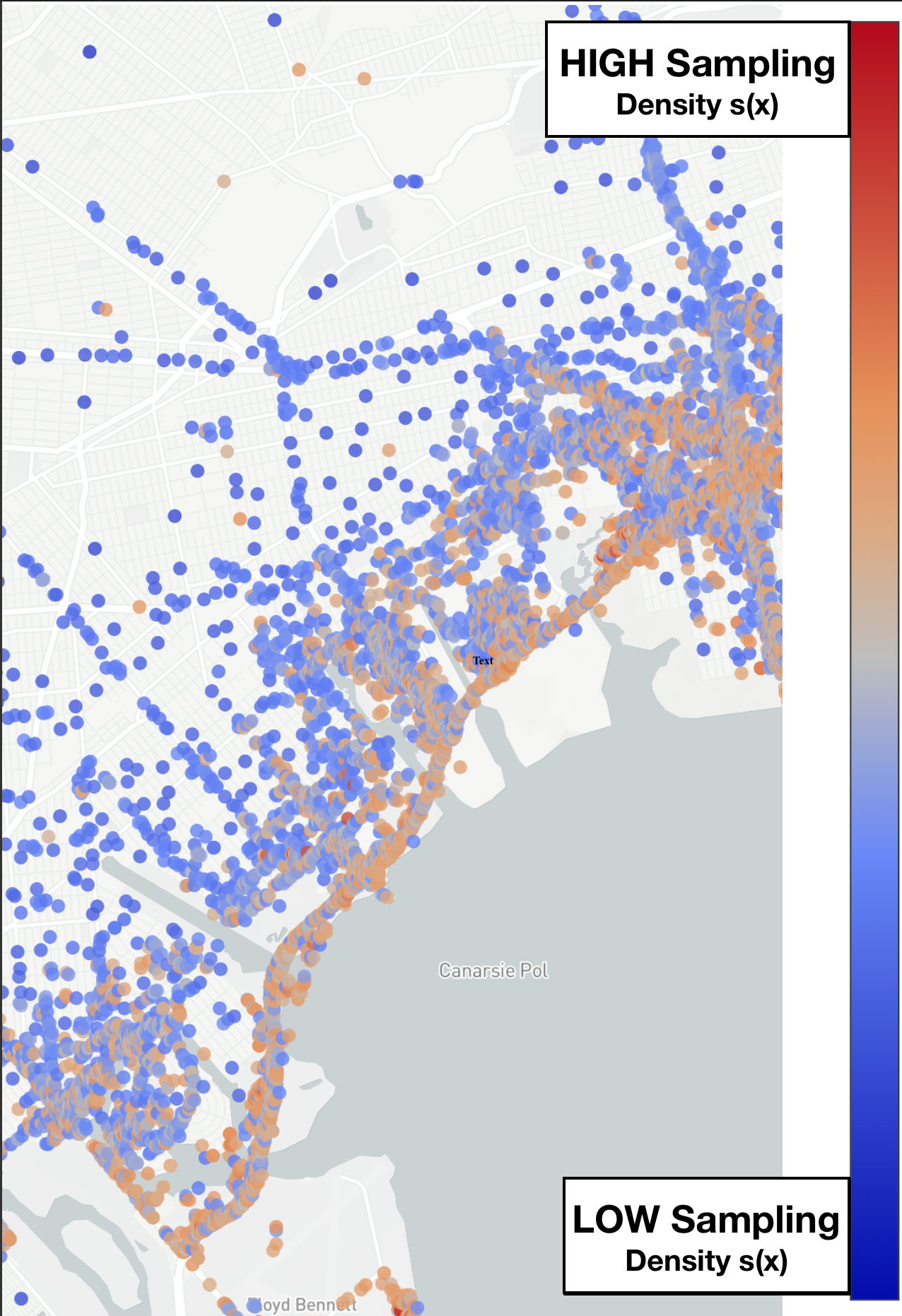
(a) Actual Measurements $s(\mathbf{l})$.

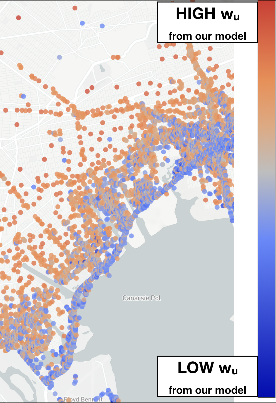
(b) Importance sampling.

Figure 11. NYC dataset: RSRP prediction and uniform error $\varepsilon_{u}$. (a) Actual sampling ($s(\mathbf{l})$) estimated by an adaptive bandwidth KDE. (b) Reweighting with $w_{u}$ from importance sampling. It can be seen that the collected data from the Mobile analytics companies oversample devices during commute (GPS Apps push locations updates - power plugged) and undersample other residential areas. (b) NYC and LA datasets: Fig. 11(a) depicts the sampling distribution $s(\mathbf{l})$ in spatial dimensions (estimated by adaptive bandwidth KDE as we described in 3.4), in East NYC nearby JFK airport. It can be observed that the data are primarily being collected on the highway (Belt Pkwy) adjacent to the sea; the sampling density is much higher compared to nearby residential blocks. Although the specifics of the data collection for NYC dataset are proprietary, we can speculate that the data collection is more frequent when the devices are plugged to power and the users utilize a location navigator app which pushes location updates to other applications; it is a common practice to minimize the impact on users’ devices  (Alimpertis and Markopoulou, 2017). Fig. 11(b) illustrates the importance ratio weights $w_{u}$ and how our model readjusts for the sampling-target distribution mismatch. Similar patterns are observed throughout many different areas in NYC and LA datasets: e.g., see the 405 highway in the Long Beach area x210. Table 10 reports the error $\varepsilon_{u}$ for different LTE TAs in NYC and LA datasets. The average performance improvement by training RFs${}_{w_{u}}$ is approx. 3%, with up to 5% in some units. We also examined the area x532 where the benefit of our method was small and as expected the spatial distribution was indeed approx. uniform (omitted for space limitations). At the other extreme, regions with highly biased data collection (i.e., x540 East NYC and x210 Long Beach in LA) show the highest error reduction (3.6% and 5.3% respectively). Overall, we find higher gains to reweighting on Campus dataset, as it is collected from a small number of users and hence more unevenly sampled. We expect that this feature will be common for small-scale data sets as well as setups with biased sampling because of mobile analytics companies practices, making reweighting especially important to correct for sampling bias. LTE-TA Characteristics $RFs$ $:\widehat{y}$ $RFs_{w_{u}}$ $:\widehat{y}_{w}$ Improvement $TAI$ $N$ Info $\sqrt{\varepsilon_{u}}$ $\sqrt{\varepsilon_{u}}$ Diff. Diff. (%) x210 197521 Long Beach Lakewood 4.06 3.84 0.21 5.3 x552 97942 Eastern Brooklyn 5.38 5.12 0.26 4.9 x540 136105 E. Long Island 5.01 4.83 0.18 3.6 x535 121159 W. Queens 5.36 5.17 0.19 3.6 x641 10663 Covina Hacienda Heights 1.8 1.74 0.06 3.5 x561 62448 Manhattan Mid. 5.64 5.46 0.18 3.2 x470 198252 LA Downtown Hollywood 4.56 4.43 0.13 2.8 x211 77049 Suburban S. LA 4.06 3.96 0.1 2.4 x442 14538 Manhattan Uptown Queens - Bronx 3.23 3.19 0.05 1.5 x537 37247 Manhattan Midtown East 7.62 7.53 0.09 1.1 x321 5111 Eastern Brooklyn 3.87 3.83 0.04 1.1 x532 136508 Brooklyn 5.46 5.43 0.03 0.5 ALL 1094543 NYC & LA 4.88 4.72 0.16 3.16 Table 10. NYC and LA datasets, RSRP $y$ prediction: $\varepsilon_{u}$ Error (i.e., reweighted according to the uniform distribution $\equiv$ $P=($$I,w_{u}$$)$): (i) Train on Default RFs vs.  (ii) train on RFs_w $w_{i}=w_{u}\propto\frac{1}{s(\mathbf{l})}$. Models per LTE TA. We use adaptive bandwidth KDE for estimating $s(\mathbf{l})$(Lichman and Smyth, 2014). Our methodology shows improvement up to $5.3\%$.

4.5.2. $\varepsilon_{P}$ : reweighting for Population Density $P=($$I,w_{d}$$)$.

Weighing errors by local population density, instead of uniformly, results in a metric that places more emphasis on accuracy in regions where more potential users reside. To that end, we utilize public APIs to retrieve the census data and estimate the population density ${d}($$\mathbf{l}_{i}$$)$. Reweighted $\varepsilon_{d}$ for RSRP data by using the weighted train RFs${}_{\text{$w_{d}$}}$ vs. the the default RFs show an improvement of up to 5.7%. Table 11 reports the error weighted proportional to the actual user population density over the same spatial area. KPI: CQI All LTE-TA regions Training Options $y$ domain $\rightarrow$ $Q(\widehat{y})$ $Q(y)$ domain $w_{i}=1,\forall i$ $Q_{cdp}(\widehat{y})$ 0.0107 $\widehat{Q}_{cdp}(y)$ 0.0088 $w_{i}=w_{P}\propto\frac{\text{${d}($$\mathbf{l}_{i}$$)$}}{s(\mathbf{l}_{i})}$ $Q_{cdp}(\widehat{y}_{w})$ 0.0109 $\widehat{Q}^{w}_{cdp}(y)$ 0.0085 Relative Difference -2.3% 3.07% KPI: RSRP All LTE-TA regions $w_{i}=1,\forall i$ $Q_{cdp}(\widehat{y})$ 0.0045 $\widehat{Q}_{cdp}(y)$ 0.0036 $w_{i}=\text{$w_{d}$}\propto\frac{\text{${d}($$\mathbf{l}_{i}$$)$}}{s(\mathbf{l}_{i})}$ $Q_{cdp}(\widehat{y}_{w})$ 0.0047 $\widehat{Q}^{w}_{cdp}(y)$ 0.0034 Relative Difference -5% 4% Table 11. NYC and LA datasets. The error $\varepsilon_{d}$  is re-weighted according to the population distribution) is computed on the $Q$ domain, i.e., $P=($$Q_{cdp},\text{$w_{d}$}$$)$. When predicting $\widehat{y}$ with weights and then converting to $Q(y)$, information is lost from the transformation. When training with the importance sampling weights, then predicting $\widehat{Q}(y)$, can further reduce the error up to $5\%$. Table 12 includes the reweighted $\varepsilon_{d}$ for RSRP data by using the default RFs vs. the weighted train RFs${}_{\text{$w_{d}$}}$ ; we see perfor- mance improvement up to 5.7 LTE-TA Characteristics $RFs$ $\rightarrow\widehat{y}$ $RFs_{w_{P}}$ $\rightarrow\widehat{y}_{w}$ Improvement $TAI$ $N$ Info Default $\sqrt{\varepsilon_{P}}$ $\sqrt{\varepsilon_{P}}$ Diff. Diff. (%) x561 63303 Manhattan Midtown 7.23 6.82 0.41 5.7 x321 7014 Eastern Brooklyn 4.94 4.8 0.14 2.8 x535 122071 W. Queens 6.03 5.87 0.15 2.5 x552 98240 Eastern Brooklyn 5.35 5.29 0.06 1.2 x532 137962 Brooklyn 6.24 6.22 0.02 0.3 x537 37964 Manhattan Midtown East 8.82 8.81 0.01 0.1 x540 138495 E. Long Island 5.09 5.09 0.00 0.0 x442 16372 Manhattan Uptown Queens - Bronx 3.97 4.21 -0.24 -6.1 ALL 621421 NYC 5.98 5.90 0.08 1.35 Table 12. NYC and LA datasets RSRP $y$ prediction: $\varepsilon_{d}$ Error (i.e., reweighted according to the population distribution): (i) Train on Default RFs vs.  (ii) train on RFs_w $w_{i}=\text{$w_{d}$}\propto\frac{\text{${d}($$\mathbf{l}$$)$}}{s(\mathbf{l})}$. Models per LTE TA. We use adaptive bandwidth KDE for estimating $s(\mathbf{l})$(Lichman and Smyth, 2014). Our methodology shows improvement up to $5.7\%$.

4.6. Reweighted Error for QoS functions: $P=(Q,W)$

So far, we have separately evaluated the improvement from (1) predicting QoS directly and (2) re-weighting by importance ratio. Here, we combine the two and calculate the reweighted error $\varepsilon_{p}$ (how we handle the input space) for a QoS function (how we handle the output space) of interest. Due to lack of space, we only show results for $Q_{cdp}($y$)$. In Table 3, we show four cases to be compared. First, $Q_{cdp}(\widehat{y})$ is the baseline, where we first predict the signal map value $y$ of interest and then get an estimate of the CDP. Second, $\widehat{Q}_{cdp}(y)$ is our prediction directly on the function of interest. Third, we can train a weighted RFs_w for $y$, and get $Q_{cdp}(\widehat{y}_{w})$. Last, we can have $\widehat{Q}^{w}_{cdp}(y)$ which is the weighted trained model RFs_w for estimating CDP (i.e., $P=($$Q_{cdp},W$$)$). Table 13 reports the errors for uniform loss over a spatial area, and shows improvements up to 5.5%. Interestingly, the baseline performance deteriorates when we train on the adjusted weights. It tries to minimize MSE for $y$, therefore the weights can have very little or even negative effect for mapping back to CDP. Similar results are observed for error proportional to user population density, but omitted due to lack of space. This demonstrates the importance of choosing the loss function, jointly controlled by $w$ and $Q$, to optimize performance for a specific prediction problem. KPI: CQI All LTE-TA regions Training Options $y$ domain $\rightarrow$ $Q(\widehat{y})$ $Q(y)$ domain $w_{i}=1,\forall i$ $Q_{cdp}(\widehat{y})$ 0.018 $\widehat{Q}_{cdp}(y)$ 0.0169 $w_{i}=w_{u}\propto\frac{1}{s(\mathbf{l}_{i})}$ $Q_{cdp}(\widehat{y_{w}})$ 0,018 $\widehat{Q}^{w}_{cdp}(y)$ 0.0160 Relative Difference 0.5% 5.5% KPI: RSRP All LTE-TA regions $w_{i}=1,\forall i$ $Q_{cdp}(\widehat{y})$ 0.028 $\widehat{Q}_{cdp}(y)$ 0.023 $w_{i}=w_{u}\propto\frac{1}{s(\mathbf{l}_{i})}$ $Q^{w}_{cdp}(\widehat{y})$ 0.029 $\widehat{Q}^{w}_{cdp}(y)$ 0.022 Relative Difference -2% 2.3% Table 13. $P=($$Q_{cdp},w_{u}$$)$, NYC and LA datasets, error $\varepsilon_{u}$ (i.e., reweighted according to the uniform distribution), results on the $Q$ domain. Predicting $\widehat{y}$ with weights and then converting to $Q(y)$ does not help because information is lost from the transformation. Predicting $\widehat{Q}(y)$ after training with the importance sampling weights further reduces error up to $5\%$.

4.7. Data Shapley Results

In this section, we compute the Data Shapley values (using the techniques presented in Section 3.5 and Appendix A1) of datapoints in our datasets. For each prediction problem $P=(Q,W)$ and dataset of interest, we compute the performance score $V$, and eventually the shapley value $\phi_{i}$ value of every measurement datapoint $i$ in that training dataset. We then order all datapoints in decreasing shapley values, and remove datapoints with negative or low values. First, we show that by removing measurements with negative Shapley values, we can actually improve the prediction performance up to 30%; the intuition is that these are noisy/erroneous measurements. Second, we show that we can further remove a large percentage of data points (up to 65%, depending on the dataset and problem $P$) with low Shapley values, while maintaining high prediction performance. The latter enables data minimization that can practically improve privacy, and can reduce the cost of collecting, storing, uploading or buying cellular measurements. Data Minimization Setup: As we described in Sec. 3.5, we utilize the TMC-Shapley algorithm to calculate the data Shapley values $\phi_{i}$ per training data point $(\text{$\mathbf{x}$}_{i},y_{i})$, for the problem of coverage indicator classification $\widehat{Q_{c}}(y)$, i.e., whether there is coverage in a location or not (as per Sec. 4.4). We remove batches of 5% of $\mathcal{D}_{train}$ starting from the least valuable (i.e., lowest $\phi_{i}$). At each step, we re-train the RFs_all model with the remaining $\mathcal{D}_{train}$ and calculate the performance of the prediction on the $\mathcal{D}_{\text{held-out}}$ data.

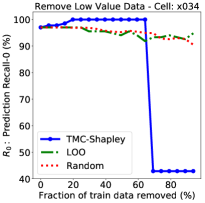
(a) Cell x$034$.

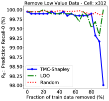
(b) Cell x$312$.

Figure 12. Campus dataset: Removing low valued data points (for Data-Shapley, LOO and Random) affects Recall $R_{0}$. Baselines for Comparison: To compare against data Shapley valuation, we consider two baselines. First, Leave-one-out (LOO) (Ghorbani and Zou, 2019), calculates the datum’s value by leaving it out and calculating the score $V$, i.e., $\phi_{i}^{\text{LOO}}=V(D)-V(D-\{i\})$. Second, we remove randomly batches of $\mathcal{D}_{train}$ at each step.

4.7.1. Effect of removing low value data on Recall.

For the Campus dataset, Figures 12(a), 12(b) and 13(a) present results for three representative cells (c034, x312, x901), in terms of the recall $R_{0}$ (see Sec. 4.4 for its utility for operators), as a function of the percentage of data removed from $\mathcal{D}_{train}$, by all discussed methods (TMC-Shapley, LOO and Random). TMC-Shapley’s performance either improves or remains the same when we remove low value data points compared to LOO and Random. There are two plausible explanations. First, the batches with low valued $\mathcal{D}_{train}$ contain outliers and corrupted data; the data Shapley has correctly identified these points compared to LOO which does not show any benefit. Second, the data points with low $\phi_{i}$ do not have much predictive power to maximize the defined performance metric of interest for the particular learning task; essentially their removal lets the best suited data points to train the predictor. Very interestingly, after a certain threshold, TMC-Shapley’s performance drops with just a removal of single batch; this subset of points (highly “influential” points) hold significant predictive power. In contrast, by removing data randomly we keep bad quality data, however we might also keep some of these “influential” points and that explains that Random’s performance neither improves nor decays fast. Let us discuss in more depth Fig.13(a), which presents data minimization results for cell x901 of the Campus dataset. The removal of low valued data according to TMC-Shapley’s valuation improves recall $R_{0}$ compared to Random and LOO. Moreover, in Fig. 13(a) we annotate with the label “A” the beginning of the process (i.e., still using the entire $\mathcal{D}_{train}$); label “B” indicates the step where $65\%$ of the data have been removed and $R_{0}$ has achieved its maximum value. Fig. 13 depicts the $\phi_{i}$ CDF values for all $\mathcal{D}_{train}$ (i.e., label “A”). Interestingly, upon closer inspection of the data, as the CDF in Fig. 13(c) shows, the data points removed between “A” and “B” have overwhelming negative values. Fig. 13(a) shows the CDF of $\phi_{i}$ at label “B” (i.e., $\mathcal{D}_{train}$ for the max $R_{0}$ achieved) and we observe that are all positive. Fig. 13(c) includes a few positive values that were removed and $R_{0}$ was keep increasing. This occurs because the TMC-Shap algorithm itself is an approximation of the closed-form data Shapley $\phi_{i}$ (eq. 6) and we relaxed the convergence rates due to the size of our datasets.

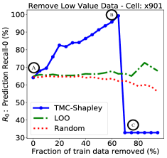
(a) Removing % Data.

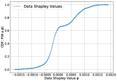
(b) Label A: all data in cell x901.

(c) data between Labels A and Label B.

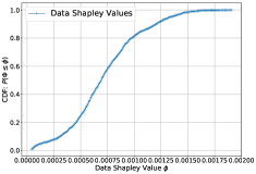
(d) Data at Label B.

Figure 13. Data minimization for Campus Cell x901. (a) Removing % datapoints using different techniques: data Shapley, Leave-One-Out, Random. As we start removing data with low data Shapley (from A to B), recall improves. If we remove more data beyond a certain point (B), recall sharply decreases (from B to C). (b)(c)(d) CDFs of Data Shapley values $\phi_{i}$ fr the points among labels A,B,C in (a). % Train Data Removed $N$ $R_{0}$ userID-0 UserID-1 0s 1s $\widehat{0}$ $\widehat{1}$ 0.0 5777 0.64 5521 256 1938 3839 541 1384 0.05 5489 0.68 5246 243 1855 3634 601 1324 0.1 5201 0.69 4967 234 1752 3449 622 1303 0.15 4913 0.76 4697 216 1651 3262 733 1192 0.2 4625 0.83 4429 196 1550 3075 889 1036 0.25 4337 0.82 4159 178 1448 2889 885 1040 0.3 4049 0.84 3882 167 1337 2712 916 1009 0.35 3761 0.84 3611 150 1226 2535 918 1007 0.4 3473 0.86 3335 138 1146 2327 1007 918 0.45 3185 0.88 3059 126 1058 2127 1062 863 0.5 2897 0.91 2780 117 976 1921 1183 742 0.55 2608 0.94 2502 107 872 1737 1274 651 0.6 2321 0.96 2226 95 768 1553 1393 532 0.65 2032 0.99 1948 85 674 1359 1631 294 0.7 1745 0.33 1671 74 585 1160 195 1730 Table 14. x901 Cell: Data Minimization Results per removal step. Table 14 reports additional detail for data minimization in cell x901, in Fig. 13(a), including: the removed fraction and number of training data, the recall $R_{0}$, number of measurements per users as well as the number of 0s and 1s of both the held-out data and the predicted $\widehat{y}$, per each step of the removal process. We make the following observations. First, for the label B, where 65% of the data have been removed and $R_{0}$ has peak at $0.99$, we notice that the predictor $\widehat{Q_{c}}(y)$ has predicted significant higher number of 0s than 1s ($1631$ 0s vs. $294$ 1s). This does not surprise us, because, the predictor $\widehat{Q_{c}}(y)$ at label B is being trained with data points of higher quality for maximizing $R_{0}$. Essentially, in this scenario, data Shapley $\phi_{i}$ encodes the ability of the data to result in training predictors that would minimize the false negatives (i.e., maximize recall) and tend to over-predict 0s than 1s. Apparently, for a different metric the low/high $\phi_{i}$ points could be different. Second, when $R_{0}$ drops from $99\%$ to $33\%$ there is still data availability for both classes and users. Dataset Shift and Data Shapley, for cell x901. The dataset shift problem (Snoek and et al., 2019) (i.e., the mismatch of the training and the target distribution) for the labels “A” vs. “C” offers also significant insights of how the final performance is affected after a certain threshold of removing training data. Fig. 14(a) shows $w_{u}\propto\frac{1}{s(\mathbf{l})}$ for the $\mathcal{D}_{train}$ data at label A; the home and work locations where data have been oversampled are illustrated clearly. The average data density is $\operatorname{\mathbb{E}}[\log s(\mathbf{l})=-3.3]$. On the contrary, Fig. 14(b) depicts $w_{u}\propto\frac{1}{s(\mathbf{l})}$ for the remaining $\mathcal{D}_{train}$ at label C and it can be clearly seen that the data distribution is closer to uniform and the average data density has been decreased to $\operatorname{\mathbb{E}}[\log s(\mathbf{l})=-9.3]$. The held-out data were randomly sampled from the original distribution, therefore, there is now a mismatch between the original and target distribution (in other words, the dataset shift problem we studied in Sec 3.4) which can explain the drop in the performance. Last but not least, the data that are being removed from label B $\rightarrow$ label C are primarily from the two oversampled regions, where we have a lot of held-out data to be tested.

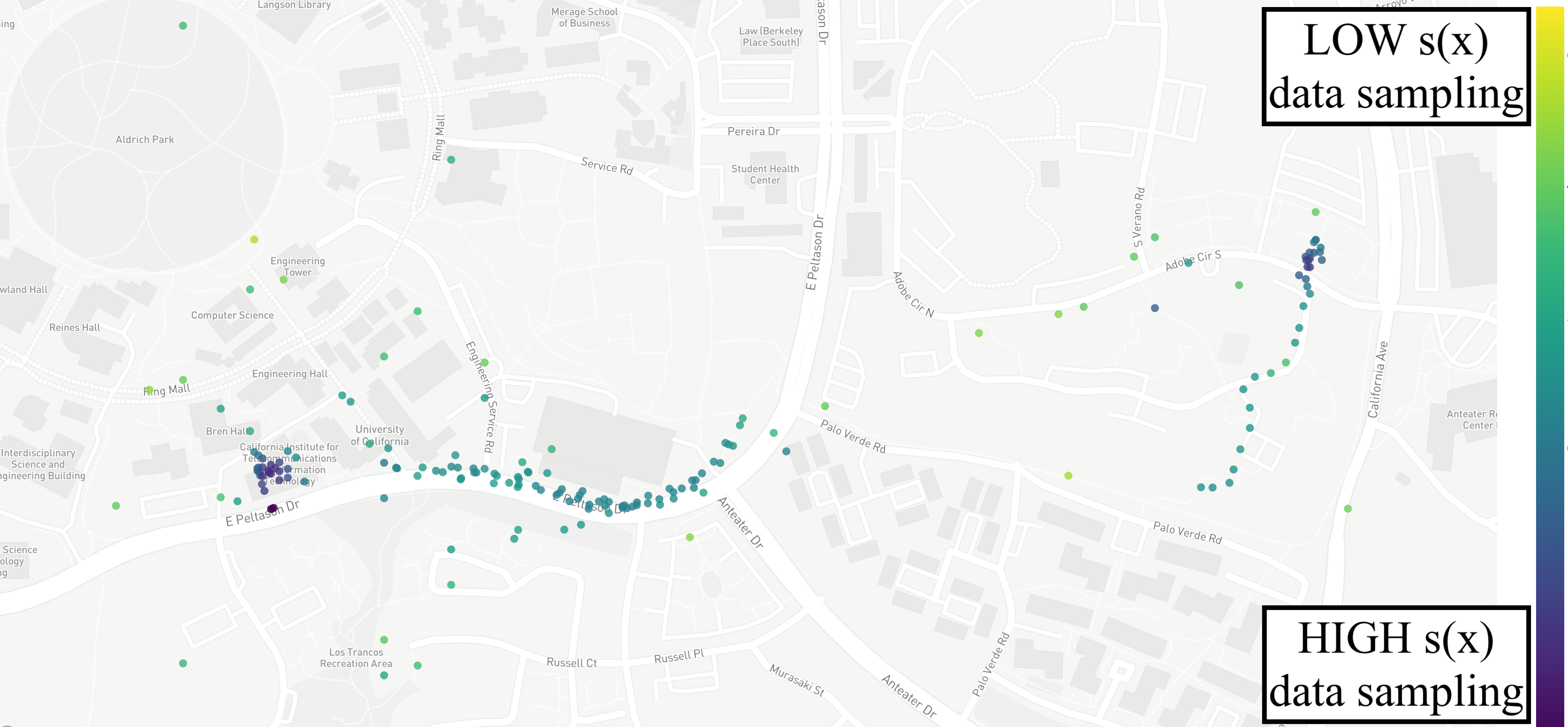
(a) Label A, Fig 13(a).

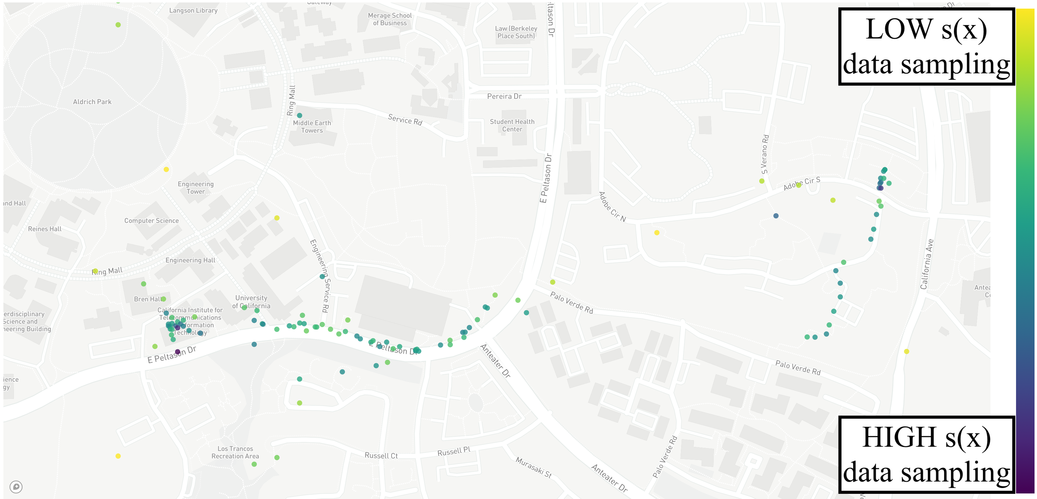
(b) Remaining Data’s $s\text{$\mathbf{x}$}$ for performance at Label C, Fig 13(a).

Figure 14. Campus dataset cell x$901$. Top: Initial Sampling distribution $s(\text{$\mathbf{x}$})$ (Data for Label A in Fig. 13(a)). $\operatorname{\mathbb{E}}[\log s(\text{$\mathbf{x}$})=-3.3]$ Bottom: Final Sampling distribution $s(\text{$\mathbf{x}$})$ (Data for Label C in Fig. 13(a)). The procedure of removing data points it eventually changed the sampling distribution of the data; at label A two regions were largely oversampled; at label C when the performance has finally been decreased the sampling distribution of the data look more uniform therefore it mismatches the original train distribution. $\operatorname{\mathbb{E}}[\log s(\text{$\mathbf{x}$})=-9.3]$ Fig. 15 shows data minimization results for cells x306 and x914.

(a) Cell x$306$.

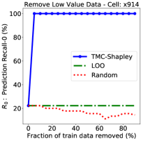
(b) Cell x$914$.

Figure 15. Campus dataset: Remove low valued data points (for Data-Shapley, LOO and Random) for various cells. Recall $R_{0}$ results.

4.7.2. Effect of Data Minimization on Metrics beyond $R_{0}$

We also considered another cell x034 and the coverage classification task, but now for a different performance metric ($V$): accuracy ($A$). Fig. 16(a) reports results from the same data removal process as previously (i.e., remove an increasing percentage of lowest valued datapoints). We observe that the TMC-Shapley’s performance eventually outperforms LOO and Random when certain threshold of data removal has been reached. However after a certain threshold, the performance of TMC-Shap drops, as happened with the recall for the same cell (Fig. 16(b)). That is expected because the portion of the data that can be removed depends on the dataset and the particular performance score/error metric, even for the same predictor.

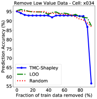
(a) Accuracy $A$.

(b) Recall $R_{0}$.

Figure 16. Campus dataset: Remove low valued data points (for Data-Shapley, LOO and Random) for cell x$034$; Left (a) Results for Accuracy, Right (b) Results for Recall $R_{0}$ for coverage loss.

4.7.3. Data Shapley with Reweigthed Error Metrics.

We further combined data Shapley and importance sampling, in order to provide data valuation for cellular operators objectives (i.e., reweigthed error metrics). For this problem $P=($$I,w_{u}$$)$, we calculate the data Shapley values $\phi_{i}$ for the performance metric of $\varepsilon_{u}$ (uniform spatial error). Fig. 17 shows a work location; in contrast to the $P_{B}=(I,k)$ the over-sampled areas have a assigned a significant lower $\phi_{i}$ score because they do not contribute much to the maximization of the performance metric $\varepsilon_{u}$.

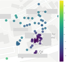
(a) $w_{u}\propto\frac{1}{s(\mathbf{l})}$.

(b) Data Shapley $\phi_{i}$; $V\leftarrow$ MSE.

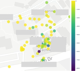
(c) Data Shapley $\phi_{i}$; $V\leftarrow\varepsilon_{u}$.

Figure 17. Example of how the reweighted error metric $\varepsilon_{u}$ affects the Data Shapley Values. (a) $w_{u}$ (i.e., inversed data sampling) You can note the oversampled work location. (b) Data Shapley values for the Mean Squared Error valuation, i.e., $P=($$I,k$$)$. (c) Data Shapley for the $\varepsilon_{u}$ performance score, i.e., reweighted MSE or $P=($$I,w_{u}$$)$. Please note how the oversampled areas (i.e., with very low weights) at the home/work locations, have been assigned super small data shapley values. The performance score-evaluation function really matters.

4.7.4. Summary

We have proposed and demonstrated how to compute Shapley values of cellular measurements used for training in cellular performance predictors for any problem $P=(Q,W)$ in our framework. This enables us to identify data points with low Shapley values, which should and can be removed for improving the prediction performance and data minimization, respectively.

5. Conclusion and Discussion

We presented a framework for predicting cellular performance from available measurements, which gives knobs to operators to express what they care most, i.e., what performance metrics, in what regimes (via quality functions $Q$), and in what locations (via weights $W$). To that end, (1) we trained directly on the $Q$ instead of the RSRP domain; (2) we used the importance ratio re-weighting to address the mismatch between target and sampling distributions; and (3) we applied the data Shapley framework to assess the value $\phi$ of available measurements for the particular prediction task $P=(Q,W)$, which in turn enables data cleaning and minimization. We evaluated these ideas on large, real-world LTE datasets and demonstrated their benefits. Our contribution lies in the framework that deals with the measurements of unequal importance. It builds on top and is independent of the underlying prediction model; in this paper, we used our state-of-the-art Random Forests predictor(Alimpertis et al., 2019), but this could be replaced by other regression (with square error loss) and classification predictors, if such become available. To the best of our knowledge, this is the first signal maps prediction paper that goes beyond RSRP and MSE minimization, and the first to introduce the data Shapley framework idea in this context. Our focus has been exclusively on improving prediction, while adding privacy-enhancing mechanisms are directions for future work. Another direction for future work is the applicability not only to LTE, but also to 5G deployment. First, our framework can naturally handle prediction over small cells, e.g., similarly to what we did in the NYC dataset, where prediction was not per cell, but across an area covered by multiple cells, (i.e., LTE TA) with $cID$ used as a feature. Second, cellular operators have aggressively pushed the sub-6GHz deployments solution because of the mmWave practical limitations (Brodkin, 2019) (e.g., range of approx. 100s meters, only line-of-sight), and sub-6Ghz deployments share the same physical layer and network characteristics with the LTE networks. Third, sampling biases will be amplified with small cells deployment and our re-weighting schema could help mitigate it. Last but not least, our weight functions $W(\mathbf{x})$ can express complex 5G operator objectives (see 3.4.1) (e.g., IoT, small cells etc.).

Acknowledgments

This work has been supported by NSF Awards 1956393, 1939237, 1900654, and 1526736. We are grateful to Tutela for sharing their city-wide datasets, to former students of our group that participated to the UCI study, and Justin Ley for discussions on the DNN models.

Appendix A1. Data Shapley Formulation - Details

This appendix extends Section 3.5 with with details on the definition of Data Shapley. Data Shapley is a framework developed in (Ghorbani and Zou, 2019), which attempts to provide an answer to the question: “How do we quantify the value of the data in an algorithmic predictions and decisions?” Data Shapley can provide us a valuation of the data (i.e., assign an arithmetic value to each data point) in the setting of supervised ML. What is an equitable measure of the value of each train data point (a.k.a. datum) $(\text{$\mathbf{x}$},y_{i})$ to the training algorithm $\mathcal{A}$? In order to answer that, we have to take a closer look to the essential ingredients of a supervised ML algorithm: (a) training data, (b) learning algorithm, (c) performance metric. The prediction is a function that depends jointly on all of them, therefore, each one of them affects the equitable measure assigned to our data. We follow the exposition and the organization of (Ghorbani and Zou, 2019); the notation of the aforementioned components is as follows: (a) Data: The dataset of the ML setting follows the typical setup we have already seen in this paper: $\mathcal{D}=\{(\text{$\mathbf{x}$}_{i},y_{i})\}^{N}_{1}$. We denote with $\mathcal{D}_{train}$ and $\mathcal{D}_{test}$ the training and the test data respectively; in the Data Shapley framework we also need $\mathcal{D}_{eval}$ for the final evaluation, i.e., the heldout data. (b) Learning Algorithm $\mathcal{A}$: A black box for the data Shapley setting, which takes as input $\mathcal{D}_{train}$ and produces as ouput a predictor $\widehat{y}=\widehat{f}_{y}(\mathbf{x})$. For example, the algorithm could be a logistic regression or the RFs predictors we used in this paper. (C) Performance Score $V$: We can treat it as a black box that takes an input $\widehat{f}$, the error metric - valuation we want to apply to each data point, the test data $\mathcal{D}_{test}$ and outputs a performance score $V$. We denote with $V(S,\mathcal{A})=V(S)$ the performance score of a predictor trained on train data $S$ using the learning algorithm $\mathcal{A}$. Please note, that the performance score can be completely different than the loss function of the learning algorithm itself. For example, we can train RFs  regression with the typical $MSE$ minimization and then report also $RMSE$ as we did in Chapter 4, however, we could train a model on a different loss function than the evaluation functions as we did in some cases in Chapter LABEL:chapter_qosweights. Data Shapley provides us a powerful framework for evaluating the different quality functions and weights functions (which essentially are other forms of error metrics according to a target distribution of interest). The goal is to compute the data Shapley value $\phi_{i}(\mathcal{D},\mathcal{A},V)\equiv\phi_{i}(V)=\phi_{i}\in\mathbb{R}~{}\forall i,(\text{$\mathbf{x}$}_{i},y_{i})\in\mathcal{D}_{train}$, which follows the equitable valuation properties described next. Equitable Valuation Conditions It is desirable that the data Shapley valuation meets the following equitable valuation conditions:  (Ghorbani and Zou, 2019): (1) Null Property. If a datum $(\text{$\mathbf{x}$}_{i},y_{i})$ does not change the performance it should be given $\phi_{i}=0$. Thus, $\forall S\subseteq\mathcal{D}-\{i\},V(S)=V(S\cup\{i\})$ (2) Symmetry Property. If two distinct datums $i,j$ contribute equally to the performance score $V$ then they should have equal data Shapley values. In other words, $\forall i,j\in\mathcal{D}$ such as $S\subseteq\mathcal{D}-\{i,j\}$ and $V(S\cup\{i\})=V(S\cup\{j\})\Rightarrow\phi_{i}=\phi_{j}$. (3) Summation and linearity. It is very typical in Machine Learning to have an overall performance score which is the sum of seperate performance scores. A typical example is the mean squared error (MSE) that is the summation of the weighted equally (i.e., the mean) squared losses of individual points. When $V$ consists of the summation of individual scores, then, the overall value of a datum should be the sum of its values for each score. In other words, for data Shapley we should have: $\phi_{i}(V+W)=\phi_{i}(V)+\phi_{i}(W)$ for performance scores $V,W$. It should be re-emphasized, that the data Shapley value is defined for the train data points according to the performance scores on the test data. Thus, $V=-\sum_{k\in test}l_{k}$ with $l_{k}$ to be the predictor’s loss on the $k$th test point; the data Shapley value for quantifying the value of the $i$th source for predicting the $k$th test point is denoted with $\phi_{i}(V_{k})$. If datum $i$ contributes values $\phi_{i}(V1)$ and $\phi_{i}(V_{2})$ to the predictors of the test points 1 and 2 respectively, then we expect the data Shapley value of $i$ in predicting both test points, i.e., when $V=V_{1}+V_{2}$, to be $\phi_{i}(V_{1})+\phi_{i}(V_{2})$. Closed Formula and Approximation. The data Shapley value which complies to the above three properties, must have the following closed form (Ghorbani and Zou, 2019): (6) $\displaystyle\phi_{i}=C\sum_{\mathcal{D}-\{i\}}\frac{V(S\cup\{i\})-V(S)}{\binom{n-1}{|S|}}$ Intuitively, a data point interacts and influences the training procedure, which creates the predictor function, in conjunction with the other training points. Thus, conditions which formulate the interactions among the data points and how an holistic data valuation is generated should be taken into account. The data Shapley value in Eq. (6) is essentially the average of the leave-one-out value (a.k.a. marginal contributions) of all possible training subsets of data in $S$. It should be noted that an exhaustive computation of Eq. (6) is very expensive computationally. An approximation - truncated Monte Carlo algorithm (TMC-Shapley) is provided by (Ghorbani and Zou, 2019) and is being used in this paper. Leave-one-out (LOO) Baseline. A simpler method is “leave-one-out” (or LOO), which calculates the datum value by leaving it out and calculating the performance score, i.e., $\phi_{i}^{\text{LOO}}=V(D)-V(D-\{i\})$. However, LOO does not consider all possible subsets a data point may belong and does not satisfy the equitable conditions.

Appendix A2. Choice of Base Predictor

This appendix extends Sections 3.2 and 4.3 (e.g., it elaborates on the comparison in Table 6), and provides additional evaluation results to justify the choice of RFs  as a good predictor for the base model $P=(I,k)$, underlying our framework. In our short paper (Alimpertis et al., 2019), we had compared RFs to model-based (LDPL) and spatiotemporal predictors (OK, OKD). In this appendix, we added a comparison to state-of-the-art DNN and CNN baselines, which have appeared after (Alimpertis et al., 2019). However, this is background information for completeness, and not the core contribution of this paper.

A2.1 Random Forests

We developed the Random Forests predictor in  (Alimpertis et al., 2019; Alimpertis, 2020), and we showed that it outperforms state-of-the-art predictors. In this paper, we use it as the base ”workshorse” predictor. We describe the design of the RFs predictor in Section 3.2, and we compare its performance to other candidates baseline predictors (including model-based, geospatial interpolation, and DNNs) in Section 4.3 and in this appendix. This is for completeness so that we justify that it is a good choice for base predictor. However, we emphasize that it could be replaced in our framework by any other predictor that minimizes MSE, without affecting the contributions of our framework, which build on top of any base predictor. RFs is not the contribution of this paper, thus its performance evaluation is mostly in this appendix (except for the summary in Table 6, which is in the main paper).

A2.2 Other Baseline Predictors

In this section, we present representative state-of-the-art prediction methods, which are used as baselines in this paper. Table 1 summarizes the family of predictors that can be used to generate coverage maps as well as put our proposed work into perspective. There is a large literature on propagation models (Bultitude and Rautiainen, 2007; Yun and Iskander, 2015; Report, 1999) and they model the received signal strength given the location of receiver, transmitter and the propagation environment. As a representative baseline from the family of model-based predictors, we consider the Log Distance Path Loss (LDPL) propagation model, which is simple yet widely adopted in the literature. Additionally, it provides further understanding of the (i) low-level RSS statistical properties and (ii) the wireless network fundamentals that should be taken into account for the prediction task.

A2.2.1 Model Based Prediction (LDPL)

The Log Distance Path Loss (LDPL) model predicts the power (in dBm) at location $\mathbf{l}_{j}$ at distance $||\mathbf{l}_{\text{BS}}-\mathbf{l}_{j}||_{2}$ from the transmitting basestation (BS) or cell tower, as a log-normal random variable (i.e., normal in dBm) (Rappaport, 2001; Alimpertis et al., 2014): (7) $\displaystyle y_{\text{$cID$}}^{(t)}\left(\mathbf{l}_{j}\right)=P_{0}^{(t)}-10n_{j}\log_{10}\left(\frac{||\mathbf{l}_{\text{BS}}-\mathbf{l}_{j}||_{2}}{d_{0}}\right)+\omega_{j}^{(t)}.$ The most important parameter is $n_{j}$, i.e., the path loss exponent (PLE), which has typical values between 2 and 6. $P_{0}^{(t)}$ is the received power at reference distance $d_{0}$, which is calculated by using the free-space path loss (Friis) transmission equation for the corresponding downlink frequency, gain and antenna directionality, and $\mathbf{l}_{\text{BS}}$ the location of the transmitting antenna. In its simplest form, the equation assumes antenna reception gain and base station antenna gain equal to $0$ dBi, but the application of an antenna directionality gain model as well as mobile gain model is also possible as shown in (Alimpertis et al., 2014). The log-normal shadowing is modeled by $\omega_{j}^{(t)}\sim\mathcal{N}(0,\sigma^{2}_{j}(t))$ (in dB), with variance $\sigma^{2}_{j}(t)$ assumed independent across different locations. The cell (identified by cell ID $cID$) affects several parameters in Eq. 7, including $P_{0},\omega_{j}$, the locations of transmitting ($\mathbf{l}_{\text{BS}}$) and receiving ($\mathbf{l}_{j}$) antennas. The simplicity of this model lies in that it has only one parameter (the path loss exponent $n_{j}$) to be estimated from the measurements. Prior work (Alimpertis et al., 2014) has shown that the PLE values and the time variant RSS variance ($\sigma^{2}_{j}(t)$) can be estimated by a large number of collected measurements. It should be noted, that in real world setups, base stations’ transmission power changes according to the network load and conditions (Alimpertis et al., 2014), contributing to the time varying component of the equation. We consider two cases. Homogeneous LDPL: Much of the literature assumes that PLE $n_{j}$ is the same across all locations. We can estimate it from Eq. (7) from all the training data points. Heterogeneous LDPL-knn: Recent work (e.g.,  (Chakraborty et al., [n.d.]; Alimpertis et al., 2014)) has considered that PLE changes across different locations. We considered various ways to partition the area into regions with different PLEs, and we present the one where we estimate $\widehat{n_{j}}$ via $knn$ regression, from the $k$ nearest neighbors, weighted according to their Euclidean distance (refer to as “LDPL-knn”). Baseline LDPL  Setup. The baseline LDPL, whose performance is reported in Table 6, refers to the following parameters of Eq. (7): we compute the distance from the base station using the online database from opencellid.org; breaking distance $d_{0}=1m$ (Alimpertis et al., 2014); $freq_{dl}$ is obtained from the $EARFCN$ measurement readily available via the Android API. . In addition, for LDPL-knn: we select empirically $k=100$ neighbors for the Campus dataset and $k=10\%$ of the training data points in each cell for the NYC and LA datasets.

A2.2.2 Geospatial Interpolation (OK-OKD)

State-of-the-art approaches in data-driven RSS prediction  (Chakraborty et al., [n.d.]; Molinari et al., 2015; Phillips et al., 2012) have primarily relied on geospatial interpolation (a.k.a. geostatistics), as presented earlier in Sec. 2. However, this approach is inherently limited to predicting RSS from spatial features $(l^{x},l^{y})$ and does not naturally extend to additional dimensions and contextual information. In this section, we present the best representatives of this family of predictors, namely ordinary kriging (OK) (Molinari et al., 2015) and its variants OK detrending (OKD) (Chakraborty et al., [n.d.]), which are used as baselines for comparison in this paper. Ordinary Kriging (OK): It predicts RSS at the testing location $\mathbf{l}_{j}=(l_{j}^{x},l_{j}^{y})$ as a weighted average of the $K$ nearest measurements in the training set: $y_{j}=\sum^{K}_{i=1}\lambda_{i}y_{i}$. The weights $\lambda_{i}$ are estimated by solving a system of linear equations that correlate the test with the training data via the semivariogram function $\gamma(h)$, which defines the variance between two different data points. Semivariogram $\gamma(h)$ must be estimated by the training data for different values of the lag $h$ (i.e., the distance between the data points) and each different environment requires different $\gamma(h)$; i.e., distinct $\gamma(h)$ for Campus and NYC and LA datasets. The solution of the system is given by a Lagrange multiplier; more details for the derivation can be found in (Chakraborty et al., [n.d.]). Ordinary Kriging Partitioning (OKP): In (Chakraborty et al., [n.d.]), Voronoi-based partitioning was used to identify regions with the same PLE and apply a different OK model in each region. This is comparable to the heterogeneous propagation model. However, OKP solves separately a different optimization problem for each local subregion, which make them impractical for city wide signal maps. Ordinary Kriging Detrending (OKD) (Chakraborty et al., [n.d.]): While OK typically assumes the same mean value across locations, this does not necessarily hold for RSS values. OKD incorporates a simplified version of LDPL in the prediction in order to address this issue (Chakraborty et al., [n.d.]). This can be thought as a hybrid approach of data-driven (geospatial) and model-driven (LDPL). It is the best representative of the geospatial predictors and serves as our baseline for comparison. The basic steps of OKD are as follows: (i) OKD needs a transmitter location (we can use the strongest RSS algorirthm (Yang et al., 2010) or the OpenCellID online DB) and computes the perceived path-loss exponent $n_{i}$ at each training data point ($n_{i}=P_{0}-\text{$y^{P}$}_{i}/\log_{10}d_{i}$ , where $d_{i}=||\mathbf{l}_{\text{BS}}-\mathbf{l}_{i}||_{2}$). (ii) After computing the mean PLE $\widehat{n}$, OKD computes $L(y_{i})=y_{i}-10\widehat{n}\log_{10}(d_{i})$ and the detrending component $\delta_{i}=y_{i}-L(y^{P}_{i})$ for the training data points. (iii) Finally, OKD applies OK to predict $\delta_{j}$ by learning with the data $\delta_{i}$ and predicts $\delta_{j}$. Baseline Geostatistics Setup. For the evaluation of geostatistics predictors reported in Table 6, we choose the following configuration. The number of neighbors was empirically set to $k=10$. For geospatial interpolation methods, a larger $k$ did not show any significant improvement, and it would result in much higher computational cost. An exponential fitting function of the semivariogram function $\gamma(h)$ was selected (Chakraborty et al., [n.d.]); the maximum lag ($h$) was set to $200$m, as in (Chakraborty et al., [n.d.]), for the Campus and NYC environments, while it was set to $600$m for the LA suburban environment. The approximated empirical semivariogram $\widehat{\gamma(h)}$ was calculated per $10m$ (Chakraborty et al., [n.d.]).

A2.2.3 Deep Neural Networks (DNNs)

In our effort to pick a state-of-the-art baseline model, we considered and evaluated the following approaches. Recent work in (Enami et al., 2018) uses DNNs along with detailed 3D maps from Light and Range Detection Data (Li-DAR) and spatial coordinates $\mathbf{l}_{j}=(l_{j}^{x},l_{j}^{y})$ as features for predicting signal strength (LTE RSRP) values. In our paper, we compare our RFs predictors with a DNN predictor. It should be noted that we only consider spatial coordinates since they are not Li-DAR readily available for our datasets. Most importantly, Li-DAR data are expensive and difficult to obtain. Our paper focuses on developing predictors with readily available data from the mobile devices provided by Android APIs. We also did a straw man evaluation of a state-of-the-art CNN approach (Krijestorac et al., 2020). We usied a simplified implementation based on the source code kindly provided by the authors of (Krijestorac et al., 2020), and tried two datasets: (i) the same synthetically generated data as in (Krijestorac et al., 2020) and (ii) on own real-world UCI campus data. Specifically, we used the synthetic data to construct ground truth masks that matched the UCI campus masks and then trained the CNNs with the original masks and our real-world sparse masks. The second option resulting to much lower performance due to data sparsity in our case. DNN Baseline Setup. The baseline “DNN”, whose performance is reported in Table 6, refers to the following configuration. We tuned the multilayer perceptron deep neural network (DNN) architecture for each cell tower via the Keras Hyperband Tuner (et al., 2019, 2018) which is an optimized version of random search. Specifically, we tuned the width (1024 nodes max.) and depth (4 layers max.) of each DNN, the activation functions, dropout percentage (0.25 max.) and used the Xavier normal weight initializer (Glorot and Bengio, 2010). We also added batch normalization which did not decrease the RMSE. After tuning the architecture, we re-train and test each cell DNN on five independent random splits of data and report the average performance.

A2.4 Baseline Models Comparison

Figure 18. Campus dataset: $RMSE$ vs. Training Size. Our methodology (RFs with more than spatial features, i.e., RFs_x,y,t, RFs_all) significantly improves the RMSE-cost tradeoff: it can reduce $RMSE$ by $17\%$ for the same number of measurements compared to state-of-the-art data-driven predictors(OKD); or it can achieve the lowest error possible by OKD ($\simeq 2.8$dB) with 10% instead of 90% (and 80% reduction) of the measurements. a. Campus dataset: Table 6 reports the $RMSE$ for all predictors for each cell in the Campus dataset, for the default 70-30% split. Fig. 20 compares all methods, calculating $RMSE$ over the entire Campus dataset, instead of per cell. We can see that our RFs-based predictors (RFs_x,y,t, RFs_all) outperform model-based (LDPL) and other data-driven (OK, OKD, DNN) predictors. Fig. 18 shows the $RMSE$ as a function of the training size (as % of all measurements in the dataset). First, the performance of OK and RFs_x,y is almost identical, as it can be seen for $RMSE$ over all measurements (Fig. 18 and Fig. 20) and $RMSE$ per cell (Table 6). This result can be explained by the fact that both predictors are essentially a weighted average of their nearby measurements, although they achieve that in a different way: OK finds the weights by solving an optimization problem while RFs_x,y uses multiple decision trees and data splits. Second and more importantly, considering additional features can significantly reduce the error. For the Campus dataset, when time features $\mathbf{t}=(d,h)$ are added, RFs_x,y,t significantly outperforms OKD: it decreases $RMSE$ from $0.7$ up to $1.2$ dB. Alternatively, in terms of training size, RFs_x,y,t needs only $10\%$ of the data for training, in order to achieve OKD’s lowest error ($\simeq 2.8$dB) with $90\%$ of the measurement data for training. Our methodology achieves the lowest error of state-of-the-art geospatial predictors with $80\%$ less measurements. The absolute relative improvement of RFs_x,y,t compared to OKD is $17\%$, shown in Fig. 20(b). b. NYC and LA datasets: Fig. 19 shows the error for two different LTE TAs, namely for NYC Manhattan Midtown (urban) and for southern LA (suburban), where RFs have been trained per $cID$. CDFs of the error per $cID$ of the same LTE TA are plotted for different predictors. Again, OK performance is very close to RFs_x,y, because they both exploit spatial features. However, RFs_all with the rich set of features improves by approx. $2$dB over the baselines for the 90th percentile, in both LTE TAs. Interestingly, the feature $dev$  is important, which is expected since this data, has heterogeneous devices reporting RSRP. Prior work has ignored important device, radio frequency and hardware’s receiver information. First, each device calculates its signal strength (e.g., LTE RSRP) differently (i.e., proprietary algorithm in the device’s cellular modem, since 3GPP just provides generic guidelines). Second, receiving sensitivity (the minimum RSRP for a feasible wireless communication) changes per device because each wireless receiver has different noise figure (NF) (Alimpertis et al., 2014). In sharp contrast to prior art, our RFs-based predictor inherently considers this feature. There are multiple reasons why RFs_all outperform geospatial interpolation predictors. The mean and variance of RSRP depend on time and location and the complex propagation environment. RFs can easily capture these dimensions instead of modeling a priori every single aspect. For example, RFs_x,y,t predicts a time-varying value for the measurements at the same location in Fig. 5(a), while RFs_x,y or OK/OKD produce just a flat line over time. OK also relies on some assumptions (same mean over space, semivariogram depending only on the distance between two locations), which do not hold for RSRP. Even hybrid geospatial techniques (OKD) cannot naturally incorporate additional features (e.g., time, device type, etc. ). Finally, RFs significantly outperform propagation models.

(a) NYC Manhattan Midtown

(b) LA Southern Suburb

Figure 19. NYC and LA datasets: CDFs for $RMSE$ per $cID$  for two different LTE TAs, for the same major MNCarrier-1. RFs_all  offer $2$dB gain over the baselines for the 90th percentile. Similarly, the RFs-based predictors outperform the DNN-based predictor. First, DNNs cannot handle efficiently the disjoint regions and discontinuous values of the RSRP values as RFs inherently do (e.g., in Fig. 3). Second, DNNs need a huge amount of data in order to perform well with discontinuous and non smooth functions. Furthermore, more complex architectures of DNNs would be needed along with very specialized and expensive to obtain features such as Li-DAR data, 3D building models etc.  (Enami et al., 2018). Finally, DNNs need normalized input, which has significant effects on latitude/longitude values, and cannot support both categorical and continuous features. Figure 20. Comparison of ARI for each predictor over the entire Campus dataset. Our Approaches (RFs_x,y,t, RFs_all) outperform prior art in all scenarios. We refer to our prior work in (Alimpertis et al., 2019) for an extensive presentation of the MSE minimization, $P=($I,k$)$, where we considered: (i) The feature importance, (ii) the RFs model granularity, (iii) the differences between urban vs. suburban environments and (iv) the location density and we show how the RFs  do not overfit. For the rest of the paper, the focus is the prediction problem beyond MSE (i.e., $P=($Q,k$)$, $P=($I,W$)$ $P=($Q,W$)$ and data Shapley valuation for data minimization.