A Flexible Divergence Elimination Method for Calculating Lepton Magnetic Moments in Quantum Electrodynamics

Abstract

A precise calculation of the lepton anomalous magnetic moments (AMM) requires an evaluation of the quantum electrodynamics (QED) Feynman diagrams up to five independent loops. The complicated structure of ultraviolet (UV), infrared (IR) and mixed divergences in the corresponding integrals makes it difficult to calculate these high-order contributions in reasonable computer time frame.

We demonstrate a method that eliminates all divergences point by point in Feynman parametric space (before integration) and possesses a flexibility that can be used for improving the precision of the numerical integration. This flexibility is especially actual for calculating the contributions of the Feynman diagrams with electron loops to the muon AMM. 3-loop and 4-loop numerical test results are provided.

The subtraction procedure is based on a forest formula with linear operators applied to the Feynman amplitudes of UV divergent subdiagrams. It is similar to BPHZ; the difference is in the linear operators used and in the way of combining them. It is equivalent to the on-shell renormalization after summation over diagrams: no residual renormalization is required.

1 Introduction

The electron and muon anomalous magnetic moments are measured with very high precision. The values

$$a_{e}[\text{expt.}] =0.001\,159\,652\,180\,73(28),$$

$$a_{\mu}[\text{expt.}] =0.001\,165\,920\,61(41)$$

are given in  [1] and  [2], respectively. The Standard Model theoretical predictions for $a_{e}$ use the following representation:

$$a_{e}=a_{e}(\text{QED})+a_{e}(\text{hadronic})+a_{e}(\text{electroweak}),$$

$$a_{e}(\text{QED})=\sum_{n\geq 1}\left(\frac{\alpha}{\pi}\right)^{n}a_{e}^{2n},$$

$$a_{e}^{2n}=A_{1}^{(2n)}+A_{2}^{(2n)}(m_{e}/m_{\mu})+A_{2}^{(2n)}(m_{e}/m_{\tau})+A_{3}^{(2n)}(m_{e}/m_{\mu},m_{e}/m_{\tau}),$$

where $m_{e},m_{\mu},m_{\tau}$ are the masses of the electron, muon, and tau-lepton, $\alpha$ is the fine-structure constant. An analogous formula can be written for $a_{\mu}$. Different parts of these expressions were calculated by different researchers. The current theoretical value of $a_{e}$ is in agreement with the experiment, but there is a discrepancy about $4.2\sigma$ in $a_{\mu}$. The term $A_{1}^{(10)}$ is not double-checked yet, and a significant error in this term can affect the relationship between the theory and experiment for $a_{e}$. In 2019 the author recalculated the contribution of all Feynman diagrams without lepton loops to $A_{1}^{(10)}$  [6] and discovered a discrepancy about $4.8\sigma$ with the previously known value [4]. See details about the relationship between these calculations and different measurements of $\alpha$ in  [7]. The muon value $a_{\mu}$ is more sensitive to the hadronic corrections, but the value of $A_{2}^{(10)}(m_{\mu}/m_{e})$ presented in  [8] is not double-checked yet, and a significant error in it still can be sensitive in experiments.

2 Old and new (flexible) method

The on-shell renormalization removes all divergences in the QED terms of the lepton magnetic moments. However, the renormalization applied in place leaves individual diagrams IR divergent starting with two loops  [9].

There are several methods of removing divergences before integration suitable for calculation of the QED contributions to the lepton magnetic moments  [10, 11, 12, 13]. Those methods remove divergences point by point in Feynman parametric space.

Our subtraction procedure presented in 2016  [14] will be referred to as the old method. That method has some advantages and was used in the above mentioned 5-loop calculation  [6]. It uses the Feynman parameters as well. If by $N_{l}$ and $N_{\gamma}$ we denote the number of external lepton and photon lines of a diagram, in QED we have four types of UV divergent subdiagrams: vertex-like ($N_{l}=2,N_{\gamma}=1$), electron self-energy ($N_{l}=2,N_{\gamma}=0$), photon self-energy ($N_{l}=0,N_{\gamma}=2$), photon-photon scattering ($N_{l}=0,N_{\gamma}=4$). The old method uses the following three linear operators applied to the Feynman amplitudes of UV divergent subdiagrams:

• $A$ is the anomalous magnetic moment projector (multiplied by the Dirac matrix $\gamma_{\mu}$) applied to vertex-like Feynman amplitudes;

• $U$ is an intermediate operator defined as

  $$U\Gamma_{\mu}(p,q)=a(m^{2})\gamma_{\mu},\quad U\Sigma(p)=r(m^{2})+s(m^{2})\not{p},$$

  where $\Gamma_{\mu}(p,q)$ and $\Sigma(p)$ are vertex-like and lepton self-energy Feynman amplitudes,

  $$\Gamma_{\mu}(p,0)=a(p^{2})\gamma_{\mu}+b(p^{2})p_{\mu}+c(p^{2})\not{p}p_{\mu}+d(p^{2})(\not{p}\gamma_{\mu}-\gamma_{\mu}\not{p}),\quad\Sigma(p)=r(p^{2})+s(p^{2})\not{p},$$ (1)

  $m$ – is the mass of the external lepton for this subdiagram; we use the metric tensor $g_{\mu\nu}$ such that $g_{00}=1$, $g_{11}=g_{22}=g_{33}=-1$. For the other types of UV divergent subdiagrams $U$ is defined as the Taylor expansion around zero momenta up to the needed order (for UV divergence elimination);

• $L$ is the on-shell renormalization projector applied to vertex-like Feynman amplitudes:

  $$L\Gamma_{\mu}(p,q)=[a(m^{2})+b(m^{2})m+c(m^{2})m^{2}]\gamma_{\mu}.$$

See the complete definitions in  [14]. The old method is a fixed subtraction procedure with the fixed operators $A$, $L$, $U$.

The new method was first formulated in  [7]. It uses four operators $U_{0},U_{1},U_{2},U_{3}$ instead of $U$; the operators $U_{1},U_{2},U_{3}$ are not fixed, but are given by requirements; see a preliminary (not complete) list of requirements in  [7]. Also, these operators may be different for different types of subdiagram external leptons. The divergence subtraction procedure is an object of a very accurate tuning, and it is difficult to describe all possible freedom in the procedure, because it must remove all divergences in each individual diagram (including mixed UV-IR divergences) and simultaneously it must be equivalent to the on-shell renormalization.

Let $G$ be a Feynman diagram contributing to the lepton AMM. By $\mathfrak{I}^{\prime}[G]$ we denote the set of all vertex-like subgraphs of $G$ (including $G$) lying on the main path of $G$ and having the external photon of $G$. By $\mathfrak{F}[G]$ we denote the set of all forests of UV-divergent subdiagrams of $G$ containing $G$. The expression for subtraction and extraction of AMM is

$$\sum_{\begin{subarray}{c}F=\{G_{1},\ldots,G_{n}\}\in\mathfrak{F}[G]\\ G^{\prime}\in\mathfrak{I}^{\prime}[G]\cap F\end{subarray}}(-1)^{n-1}M^{G^{\prime}}_{G_{1}}M^{G^{\prime}}_{G_{2}}\ldots M^{G^{\prime}}_{G_{n}}.$$

Here $M^{G^{\prime}}_{G^{\prime\prime}}$ equals $A_{G^{\prime\prime}}$, if $G^{\prime\prime}=G^{\prime}$; $L_{G^{\prime\prime}}-(U_{1})_{G^{\prime\prime}}$, if $G^{\prime\prime}=G\neq G^{\prime}$; $L_{G^{\prime\prime}}$, if $G^{\prime}\subset G^{\prime\prime}\subset G$; $(U_{0})_{G^{\prime\prime}}$, if $G^{\prime\prime}$ is a photon self-energy or a photon-photon subgraph. In the remaining cases it equals $(U_{2})_{G^{\prime\prime}}$, if $G^{\prime\prime}$ lies on a lepton loop; $(U_{w})_{G^{\prime\prime}}$, if $G^{\prime\prime}\in\mathfrak{I}^{\prime}[G]$ and $G^{\prime\prime}\subset G^{\prime}$; $(U_{1})_{G^{\prime\prime}}$ in the other cases; here $w=3$, if $G$ has its external photon on a lepton loop, $w=1$ otherwise. We should take the coefficient before $\gamma_{\mu}$ after applying the expression. $U_{0}$ is defined as the Taylor expansion around zero momenta up to the needed order ($2$ for photon self-energy, $0$ for photon-photon scattering); we can also use other known treatments of photon self-energy subdiagrams.

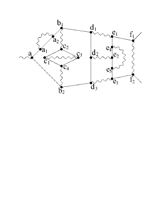
Figure 1: An example of a Feynman diagram contributing to AMM.

For example, the diagram $G$ from Figure 1 gives the expression

$$\left[A_{G}\left(1-(U_{3})_{G_{e}}\right)-\left(L_{G}-(U_{1})_{G}\right)A_{G_{e}}\right]\times\left(1-(U_{2})_{G_{c}}\right)\times\left(1-(U_{1})_{e_{2}e_{4}e_{5}}\right)$$

$$\times\left(1-(U_{0})_{G_{d}}\right)\times\left(1-(U_{0})_{c_{1}c_{2}c_{3}c_{4}}\right)\times\left(1-(U_{2})_{c_{1}c_{2}c_{3}}-(U_{2})_{c_{1}c_{3}c_{4}}\right)\times\left(1-(U_{2})_{a_{1}a_{2}}\right),$$

where $G_{e}=aa_{1}a_{2}b_{1}b_{2}c_{1}c_{2}c_{3}c_{4}d_{1}d_{2}d_{3}e_{1}e_{2}e_{3}e_{4}e_{5}$, $G_{d}=\{aa_{1}a_{2}b_{1}b_{2}c_{1}c_{2}c_{3}c_{4}d_{1}d_{2}d_{3}\}$, $G_{c}=aa_{1}a_{2}b_{1}b_{2}c_{1}c_{2}c_{3}c_{4}$, $\mathfrak{I}^{\prime}[G]=\{G_{e},G\}$, subdiagrams are denoted by enumeration of their internal vertices; we should expand brackets for obtaining the forest formula. The expression for this example does not depend on the type of leptons on lepton loops (however, each of the operators $U_{1},U_{2},U_{3}$ can be defined differently for different types of leptons).

The algorithm of calculating a diagram set contribution to the lepton AMM looks as follows:

• For the given Feynman diagram introduce the Schwinger parametric propagators

  $$(\not{p}+m)\exp(i\alpha_{j}(p^{2}-m^{2}+i\varepsilon)),\quad ig_{\mu\nu}\exp(i\alpha_{j}(p^{2}+i\varepsilon))$$

  for the lepton and photon lines, respectively, where $\alpha_{j}$ is the parameter corresponding to $j$-th internal line, $\varepsilon>0$ is an infrared regulator.

• Write the expression with linear operators (defined above) and obtain the result of applying this expression as a function of $\alpha_{1},\ldots,\alpha_{n},\varepsilon$ (by using known explicit formulas for integrals of multidimensional gaussian functions multiplied by polynomials ignoring the integral divergence; in the case of nested subdiagrams with operators, we can replace the subdiagram Feynman amplitudes with their images under the corresponding operators sequentially from smaller to larger subdiagrams).

• Obtain the result of applying the expression as a function of the Feynman parameters $z_{1},\ldots,z_{n}$ and $\varepsilon$ (taking into account the known relationship between the Schwinger and Feynman parameters, we should only make the change of variables $\alpha_{j}=\lambda z_{j}$ and perform the intergration over $\lambda$ (from $0$ to $+\infty$) analytically).

• Take the limit $\varepsilon\rightarrow+0$ (analytically).

• Integrate over $z_{1},\ldots,z_{n}$ numerically ($z_{j}\geq 0$, $z_{1}+\ldots+z_{n}=1$).

• Calculate the sum over all needed Feynman diagrams.

The details of the algorithm are described in  [14].

3 Tests and discussion

We will use the operators $U_{j}$, $j=1,2,3$ of the form

$$U_{j}\Gamma(p,q)=a(M^{2})\gamma_{\mu},\quad U_{j}\Sigma(p)=r(m^{2})+s(m^{2})m+s(M^{2})(\not{p}-m),$$

where $M^{2}$ is some subtraction point, (1) is satisfied, $m$ is the external lepton mass in the subdiagram to which the operator is applied. $U_{j}$ preserves the Ward identity and extracts the mass part of $\Sigma(p)$ completely; thus, we can consider the usage of these operators for our purposes  [7].

Since the most effective way of numerical integrating functions of many variables is the Monte Carlo method, we can compare different choices of $M^{2}$ with respect to the Monte Carlo convergence speed. If some value is obtained as the integral $\int f(z)dz$, the value $\int|f(z)|dz$ can be used as an estimation of the “badness” of $f(z)$ for Monte Carlo integration. Also, there is an observation that the contributions of individual diagrams are often “oscillating” as well as the Feynman parametric integrands [17, 6] regardless of the subtraction method used, and the oscillations are cancelled after summation over all diagrams in a gauge-invariant set. The value $\int|f(z)|dz$ (and its sum over a set) can be used as an estimation of these oscillations.

Table 1 contains the contributions of the 3-loop diagrams from Figure 2 to $A_{1}^{(6)}$ and the corresponding estimations for Monte Carlo integration obtained with $M^{2}=m^{2}$ and $M^{2}=-m^{2}$. The final results are in good agreement with each other and with the known analytical result $0.53336$. A general observation is that space-like subtraction points $M^{2}<0$ produce less oscillations than time-like ones.

Figure 2: A 3-loop gauge-invariant set.

Table 1: Contributions of the diagrams from Figure 2 to $A_{1}^{(6)}$ obtained with different subtraction points and the corresponding integrals of the absolute values.

Diagram	$M^{2}=m^{2}$, value	$M^{2}=-m^{2}$, value	$M^{2}=m^{2}$, $\int|f(z)|dz$	$M^{2}=-m^{2}$, $\int|f(z)|dz$
1	$-1.68013(35)$	$-0.97296(81)$	$2.105$	$1.394$
2	$-0.09677(49)$	$-0.6103(18)$	$1.667$	$1.311$
3	$0.21489(27)$	$-0.48545(34)$	$0.819$	$0.86$
4	$0.14480(27)$	$0.8527(27)$	$1.111$	$1.01$
5	$0.83283(40)$	$1.1325(19)$	$1.33$	$1.251$
6	$-0.02875(23)$	$0.2158(25)$	$0.666$	$0.496$
7	$0.80395(54)$	$1.10398(60)$	$1.31$	$1.173$
8	$-2.12293(27)$	$-1.2838(17)$	$2.123$	$1.318$
9	$2.52480(29)$	$1.1537(41)$	$2.587$	$1.413$
10	$-0.05880(20)$	$-0.5792(27)$	$1.084$	$1.269$
$\sum$	$0.5339(11)$	$0.5272(70)$	$14.8$	$11.49$

The contributions of the 4-loop classes IV(b) and IV(c) with an electron loop  [8] to the muon term $A_{2}^{(8)}(m_{\mu}/m_{e})$ are evaluated in Tables 2 and 3. The first table contains the evaluation with different subtraction points $M^{2}=(m_{e})^{2}$ and $M^{2}=-m_{e}m_{\mu}$. The results are in good agreement with each other and with the known values $-0.4170(37)$ and $-0.38(8)$ from  [8] and  [18], respectively. The second choice of the subtraction point produces less oscillations, this can be observed visually. The value $M^{2}=-m_{\mu}m_{e}$ is almost optimal: the selections $M^{2}=-(m_{\mu})^{2}$, $M^{2}=-m_{\mu}m_{e}$, $M^{2}=-(m_{e})^{2}$, $M^{2}=(m_{e})^{2}$ give the sums of $\int|f(z)|dz$ equal $1374$, $767$, $1113$, $1510$, respectively.

Figure 3: 4-loop gauge-invariant classes IV(b) (left) and IV(c) (right) from  [8].

Table 2: Contributions of the diagrams from IV(b) (Figure 3, left) to $A_{2}^{(8)}(m_{\mu}/m_{e})$ obtained with different subtraction points.

№	$M^{2}=(m_{e})^{2}$	$M^{2}=-m_{e}m_{\mu}$	№	$M^{2}=(m_{e})^{2}$	$M^{2}=-m_{e}m_{\mu}$
1	$32.712(73)$	$-2.753(13)$	10	$4.92(12)$	$20.465(20)$
2	$-7.118(63)$	$10.580(11)$	11	$20.817(95)$	$5.318(18)$
3	$-27.870(89)$	$7.688(17)$	12	$-7.745(98)$	$9.902(17)$
4	$-23.811(15)$	$-23.791(11)$	13	$-11.21(13)$	$4.371(27)$
5	$26.517(93)$	$11.071(18)$	14	$-19.36(11)$	$-3.791(22)$
6	$39.12(10)$	$3.642(19)$	15	$-26.433(25)$	$-26.417(11)$
7	$-23.529(21)$	$-23.522(13)$	16	$25.86(10)$	$10.431(22)$
8	$-20.30(13)$	$-4.753(22)$	$\sum$	$-0.73(37)$	$-0.340(72)$
9	$16.70(11)$	$1.221(16)$

Table 3 demonstrates an evaluation of the contribution of IV(c) to $A_{2}^{(8)}(m_{\mu}/m_{e})$ with two different combinations of the linear operators: $U_{1}=U_{2}=U,U_{3}=L$; $U_{1}=U_{2}=U_{3}=U$. The combinations give the same values for all diagrams except 7 and 8: they are the only diagrams with different expressions. However, we have a good agreement after summation between these calculations and with the known values $2.9072(44)$ from  [8] and $2.94(30)$ from  [18].

The author thanks Lidia Kalinovskaya, Gudrun Heinrich, Savely Karshenboim, Andrey Arbuzov, Andrey Kataev for the important assistance. Also, the author thanks the Laboratory of Information Technologies of JINR (Dubna, Russia) for providing an access to its computational resources and additionally the organizers of the conference ACAT-2021 for providing a possibility to make an online presentation.

Table 3: Contributions of the diagrams from IV(c) (Figure 3, right) to $A_{2}^{(8)}(m_{\mu}/m_{e})$ obtained with different selections of $U_{3}$ (we use $U_{1}=U_{2}=U$).

№	$U_{3}=L$	$U_{3}=U$	№	$U_{3}=L$	$U_{3}=U$
1	$-118.179(22)$	$-118.167(22)$	8	$20.775(32)$	$4.920(30)$
2	$91.841(21)$	$91.778(21)$	9	$100.475(24)$	$100.514(25)$
3	$-80.820(20)$	$-80.839(21)$	10	$-76.924(32)$	$-76.923(33)$
4	$2.620(22)$	$2.612(25)$	11	$89.140(31)$	$89.186(35)$
5	$-74.730(26)$	$-74.694(29)$	12	$-26.766(12)$	$-26.763(12)$
6	$37.016(22)$	$37.015(24)$	13	$-10.543(21)$	$-10.550(20)$
7	$48.934(19)$	$64.810(19)$	$\sum$	$2.840(86)$	$2.899(90)$

References

References

- [1] D. Hanneke, S. F. Hoogerheide and G. Gabrielse, “Cavity Control of a Single-Electron Quantum Cyclotron: Measuring the Electron Magnetic Moment,” Phys. Rev. A 83, 052122 (2011) doi:10.1103/PhysRevA.83.052122 [arXiv:1009.4831 [physics.atom-ph]].
- [2] B. Abi and others, “Measurement of the Positive Muon Anomalous Magnetic Moment to 0.46 ppm,” Phys. Rev. Lett. 126 (2021), 141801. doi:10.1103/PhysRevLett.126.141801 [arXiv:2104.03281 [hep-ex]]
- [3] G. W. Bennett et al, “Final report of the E821 muon anomalous magnetic moment measurement at BNL,” Phys. Rev. D 73 (2006), 072003. doi = 10.1103/PhysRevD.73.072003 [arXiv:hep-ex/0602035 [hep-ex]]
- [4] T. Aoyama, T. Kinoshita, M. Nio, “Theory of the Anomalous Magnetic Moment of the Electron”, Atoms, 7, 28 (2019). doi:10.3390/atoms7010028
- [5] T. Aoyama, N. Asmussen et al., “The anomalous magnetic moment of the muon in the Standard Model,” Physics Reports 887 (2020), 1–166. doi:10.1016/j.physrep.2020.07.006 [arXiv:2006.04822 [hep-ph]]
- [6] S. Volkov, “Calculating the five-loop QED contribution to the electron anomalous magnetic moment: Graphs without lepton loops,” Phys. Rev. D 100 (2019) no.9, 096004 doi:10.1103/PhysRevD.100.096004 [arXiv:1909.08015 [hep-ph]].
- [7] S. Volkov, “A way of fast calculating lepton magnetic moments in quantum electrodynamics” (2021), prepared for submission to PEPAN (FFK-2021 Proceedings) [arXiv:2111.00291 [hep-ph]]
- [8] T. Aoyama, M. Hayakawa, T. Kinoshita, and M. Nio, “Complete Tenth-Order QED Contribution to the Muon g-2,” Phys. Rev. Lett. 109 (2012), 111808. doi:10.1103/PhysRevLett.109.111808 [arXiv:1205.5370 [hep-ph]]
- [9] A. Petermann, “Fourth order magnetic moment of the electron,” Helv. Phys. Acta 30 (1957) 407 doi: 10.5169/seals-112823
- [10] M. J. Levine and J. Wright, “Anomalous magnetic moment of the electron,” Phys. Rev. D 8 (1973) 3171. doi:10.1103/PhysRevD.8.3171
- [11] R. Carroll and Y. P. Yao, “ contributions to the anomalous magnetic moment of an electron in the mass-operator formalism,” Phys. Lett. 48B (1974) 125. doi:10.1016/0370-2693(74)90659-5
- [12] P. Cvitanovic and T. Kinoshita, “New Approach to the Separation of Ultraviolet and Infrared Divergences of Feynman - Parametric Integrals,” Phys. Rev. D 10 (1974) 3991. doi:10.1103/PhysRevD.10.3991
- [13] T. Aoyama, M. Hayakawa, T. Kinoshita and M. Nio, “Automated calculation scheme for contributions of QED to lepton : Generating renormalized amplitudes for diagrams without lepton loops,” Nucl. Phys. B 740 (2006) 138 doi:10.1016/j.nuclphysb.2006.01.040 [hep-ph/0512288].
- [14] S. Volkov, “Subtractive procedure for calculating the anomalous electron magnetic moment in QED and its application for numerical calculation at the three-loop level”, J. Exp. Theor. Phys. (2016), V. 122, N. 6, pp. 1008–1031; in Russian: JETP (2016), V. 149, N. 6, p. 1164; doi:10.1134/S1063776116050113
- [15] G. S. Adkins, R. N. Fell and J. Sapirstein, “Two loop renormalization of Feynman gauge QED,” Phys. Rev. D 63 (2001) 125009. doi:10.1103/PhysRevD.63.125009
- [16] N. N. Bogoliubov, D. V. Shirkov, “Quantum Fields”, Benjamin/Cummings Publishing Company, 1983.
- [17] P. Cvitanović, “Asymptotic Estimates and Gauge Invariance,” Nuclear Physics B 127 (1977), 176–188. doi:10.1016/0550-3213(77)90357-1
- [18] A. Kurz, T. Liu, P. Marquard, A. V. Smirnov, V. A. Smirnov, M. Steinhauser, “Electron contribution to the muon anomalous magnetic moment at four loops,” Phys. Rev. D 93 (2016), 053017. doi:10.1103/PhysRevD.93.053017 [arXiv:1602.02785 [hep-ph]]