A Large Confirmatory Dynamic Factor Model for Stock Market Returns in Different Time Zones

Abstract

We propose a confirmatory dynamic factor model for a large number of daily returns across multiple time zones. The model has a global factor and three continental factors. We propose two estimators of the model: a quasi-maximum likelihood estimator (QML-just-identified), and an improved estimator (QML-all-res). Our estimators are consistent and asymptotically normal. In particular, the asymptotic distributions of QML-all-res are the same as those of the infeasible OLS estimators that treat factors as known and utilize all the restrictions of the parameters of the model. We apply the model to MSCI equity indices of 42 developed and emerging markets, and find that the market is more integrated when the US VIX is high.

Keywords:

Daily Global Stock Market Returns; Time-Zone Differences; Confirmatory Dynamic Factor Model; Quasi Maximum Likelihood; Expectation Maximization Algorithm.

JEL classification

C32; C55; C58; G15.

1 Introduction

Correlations among stock returns in different countries are an important ingredient of the strategic allocation decision to international stocks and for understanding the degree of segmentation of international capital markets. The last three decades have witnessed a heightening interest in measuring and modelling such correlations, whether under the rubric of stock market integration, country risk models, international stock co-movement, interdependence or otherwise. Gagnon and Karolyi (2006) and Sharma and Seth (2012) have carefully reviewed the early literature and categorized these studies according to methodologies, data sets, and findings.

The world’s stock markets are separated in time by substantial time-zone differences, to the extent that for example the American and main Asian markets do not overlap at all (although the European markets overlap a little with both the American and Asian markets). Table 1 lists the trading hours of the world’s top ten stock exchanges in terms of market capitalization on October 29th 2021. This shows the overlaps and lack of overlaps. Whenever using daily data to measure correlations, researchers have to address the issue of non-synchronous trading. This is because the closing prices of the American markets, say, contain a lot of news that could never have been in the closing prices of the Asian markets for the same calendar days (Schotman and Zalewska (2006)) and vice versa.

	Stock Exchanges	Market Cap	Trading Hours	Country
		(US trillions)	(Beijing Time)
1	New York S.E.	$26.91	21:30-04:00 ($+1$)†	US
2	NASDAQ S.E.	$23.46	21:30-04:00 ($+1$)†	US
3	Shanghai S.E.	$7.69	09:30-11:30, 13:00-15:00	China
4	Tokyo S.E.	$6.79	08:00-10:30, 11:30-14:00	Japan
5	Hong Kong S.E.	$6.02	10:00-12:30, 14:30-16:00	China
6	Shenzhen S.E.	$5.74	09:30-11:30, 13:00-15:00	China
7	London S.E.	$3.83	15:00-23:30†	UK
8	India National S.E.	$3.4	11:45-18:00	India
9	Toronto S.E.	$3.18	21:30-04:00 ($+1$)†	Canada
10	Frankfurt S.E.	$2.63	15:00-23:30†	Germany

Table 1: On October 29th 2021. ($+1$) means $+$one day. ^† means summer time.

The objective of this paper is to develop a framework to model correlations of daily stock returns in different markets across multiple time zones. This allows one to analyze international stock returns as if they were measured at the same time and location, and so allows empirical researchers to eliminate the substantial bias that would otherwise be manifested in whatever question they are addressing. The machinery will be a dynamic factor model, a special case of the generalized dynamic factor model first proposed by Forni et al. (2000). To make the model tractable, we make the following simplifying assumption: All the markets belong to one of three continents: Asia, Europe and America. We suppose that the logarithmic 24-hour close-to-close returns follow a dynamic factor model driven by both global and continental factors. This model reflects a situation in which international information represented by the global factor affects all the three continents simultaneously, but is only revealed in the returns of the three continents sequentially as their markets open in turn and trade on the new information (Koch and Koch (1991, p.235)). Local information represented by a continental factor accumulated since the last closure of that continent’s markets will also have an impact on the logarithmic 24-hour close-to-close returns of those markets in our framework. The dynamic factor structure can be consistent with a purely efficient market (if the dynamic parameter is exactly zero); it can also be consistent with market microstructure or sluggish response of prices introducing some short term autocorrelations that are presented through the dynamic evolution of the global factor.

We propose two estimators of the model: a quasi-maximum likelihood estimator (QML-just-identified), and an improved estimator (QML-all-res). A key issue here is identification and we show explicitly how to impose some of the restrictions implied by our model to guarantee identification. In particular, we impose a subset of restrictions, specifically $14^{2}$ of them. Because these $14^{2}$ restrictions cannot be written compactly in a matrix form, it took us a considerable amount of work to derive the large sample results of our estimator QML-just-identified. We next improve upon the QML-just-identified estimator and propose a QML-all-res estimator which takes all the restrictions implied by our model into account. The idea is that all these restrictions could be incorporated in an EM algorithm. Our estimators are consistent and asymptotically normal as the sample size increases. In particular, the asymptotic distributions of QML-all-res are the same as those of the infeasible OLS estimators that treat factors as known and utilize all the restrictions of the parameters of the model. We propose consistent standard errors and inference methods.

We apply our model to MSCI equity indices of 42 developed and emerging markets. Taking Asia-Pacific as an example, we find that the global factor has the largest loadings during the Asian sub-period. Mainland China and Hong Kong have large loadings on the continental factor, whereas Japan has minimal loadings on the continental factor. In addition, we adopt a methodology similar to Pukthuanthong and Roll (2009) to assess market integration. The US demonstrates the highest level of global integration but minimal regional integration. We also find evidence that the weak-form efficient market hypothesis does not hold across the globe and it takes more than a $1/3$ day for some international news to fully unfold or dissipate.

Furthermore, we investigate whether markets become more integrated during periods of high VIX. In particular, we divide the sample into four sub-samples: Before-HighVix, Before-LowVix, After-HighVix, and After-LowVix. Before-HighVix is the intersection of the before and high-VIX sub-samples, and so forth. By comparing the results between Before-HighVix and Before-LowVix (as well as between After-HighVix and After-LowVix), we find markets exhibit higher levels of integration during periods of higher VIX. This heightened integration is primarily driven by the increase of the magnitudes of loadings of the global factor during the Asian sub-period. This also means that, during periods of higher VIX, the returns of the Asian markets contain stronger trading signals for other markets.

1.1 Literature Review

There are several general approaches to address the issue of non-synchronous trading across international markets. The first approach is to use returns of relatively low frequencies: two-day returns (Forbes and Rigobon (2002), Corsetti et al. (2005), Dungey and Gajurel (2015)), weekly returns (Cappiello et al. (2006), Bekaert et al. (2009), Bekaert et al. (2014), Niţoi and Pochea (2019)), and monthly returns (Bekaert and Mehl (2019), Rapach et al. (2013)).

The second approach involves the use of intraday prices as the “pseudo” closing prices of one market to better match the closing prices of another market closing at an earlier time. For example, Schotman and Zalewska (2006) used an intraday price of the German market as its pseudo closing price when studying the German and Hungarian markets. The timing of the intraday price is chosen to match the closing time of the Hungarian market. Savva et al. (2009) and Gagnon and Karolyi (2009) also used this approach.

The third approach is attributed to Burns et al. (1998), who proposed a Vector Moving Average (VMA) structure for handling non-synchronous trading. This method has been widely utilized in various studies (Acharya et al. (2012), BenSaïda (2019), Opie and Riddiough (2020), Engle et al. (2015), Engle (2016) etc.).

The fourth approach involves using contemporaneous or lagged variables accordingly to reflect the time zone differences. For instance, Bekaert et al. (2023, p.11) wrote, “For the euro area, JP (Japanese) and EA (European) shocks that materialize before or during the European opening hours enter contemporaneously while the other shocks as well as the US shocks enter the information set on the next trading day.” Pukthuanthong and Roll (2009), Lehkonen (2015), Cai et al. (2009), He and Hamori (2021), and Marshall et al. (2021) all adopted this approach to account for non-synchronous trading.

We have a few remarks about these approaches. Using returns of relatively low frequencies as in the first approach prevents researchers from studying stock co-movement at higher frequencies. The second approach utilizes intraday data which might be unavailable or costly. The third approach is sensitive to the ordering of returns. For instance, using a vector of returns of Asia, Europe, and the US of the same calendar day might produce a different result from using a vector of returns of Europe and the US of the same calendar day, together with the return of Asia of the next day. The fourth approach is a very flexible way to address the non-synchronous trading issue, but does not allow one to identify the source of variation or its relative impacts as is possible in our framework.

The methodological approach of having global and continental factors, in some respects, is inspired by Lin et al. (1994) who investigated the correlation between the Nikkei 225 and S&P500 indices. They proposed a signal-extraction model containing a global factor and a local factor for the returns, but the model cannot generalize to a case of many stocks in multiple time zones easily. Our approach resembles that of Kose et al. (2003) who modeled 60 countries’ yearly macroeconomic aggregates (output, consumption and investment) using a dynamic factor model consisting of global, regional, and country-specific factors. The difference is that we work with daily stock returns and have the feature of sequential revelation of the international information, measured at 1/3-day frequency, in the returns of the three continents. Likewise, our approach is related to Hallin and Liška (2011) and Barigozzi et al. (2019), who considered generalized dynamic factor models in the presence of blocks, and to nowcasting (Giannone et al. (2008), Aruoba et al. (2009), Banbura et al. (2011), Banbura et al. (2013) etc.).

On the theoretical side, research about estimation of large factor models via the likelihood approach has matured over the last decade; Barigozzi (2023) provided the most recent and critical review on this topic. The likelihood approach enjoys several advantages compared to the principal components method (Banbura et al. (2013, p.204), Barigozzi (2023, p.37)). The most prominent advantage in our context (i.e., confirmatory factor models) is its flexibility to incorporate (nonlinear) restrictions on the factor loading and covariance matrices, something cannot be easily achieved in the principal components method (Stock and Watson (2016, p.431)).

Doz et al. (2012) established an average rate of convergence of the estimated factors using a maximum likelihood estimator (MLE) via the Kalman smoother. There is a rotation matrix attached to the estimated factors as the authors did not address identification of factor models. Moreover, they did not provide consistency or the limiting distributions of the loadings. In an important paper, Bai and Li (2012) took a different approach to study large exact factor models. Bai and Li (2012) obtained consistency, the rates of convergence, and the limiting distributions of the MLE of the factor loadings, idiosyncratic variances, and sample covariance matrix of factors. Factors are then estimated via a generalized least squares (GLS) method. Bai and Li (2016) generalized the results of Bai and Li (2012) to large approximate factor models.

Instead of maximizing a likelihood and finding the MLE, people usually use expectation maximization (EM) algorithms to estimate models in practice (Watson and Engle (1983), Quah and Sargent (1993), Doz et al. (2012), Rubin and Thayer (1982), Bai and Li (2012), Bai and Li (2016) etc.). Since an EM algorithm runs only for a finite number of iterations and converges to a local maximum, strictly speaking the estimate obtained by an EM algorithm is only an approximation to the MLE. However, in a breakthrough study, Barigozzi and Luciani (2022) showed that the estimate obtained by an EM algorithm, under the assumptions of their paper, converges to the MLE fast enough so that they are asymptotically equivalent.

The large sample results of the aforementioned studies are not applicable to our model because the proofs of these results are identification-scheme dependent. In particular, Bai and Li (2012), Bai and Li (2016) established their results under five popular identification schemes, none of which is consistent with our model.

1.2 Roadmap

The rest of the paper is structured as follows. Section 2 introduces the model. We explain our estimators and provide their large-sample theories in Sections 3 and 4, respectively. Section 5 conducts the Monte Carlo simulations to assess the performance of QML-all-res, and Section 6 presents empirical applications. Section 7 concludes. Additional materials and proofs are in the Online Supplement (OS in what follows).

1.3 Notation

Let $\mathbb{R}^{n}$ denote the $n$-dimensional Euclidean space. For $x\in\mathbb{R}^{n}$, let $\|x\|\mathrel{\mathop{\mathchar 58\relax}}=\sqrt{\sum_{i=1}^{n}x_{i}^{2}}$ and $\|x\|_{\infty}\mathrel{\mathop{\mathchar 58\relax}}=\max_{1\leq i\leq n}|x_{i}|$ denote the Euclidean ($\ell_{2}$) and element-wise maximum ($\ell_{\infty}$) norms, respectively. Given a vector $v$, $\operatorname*{diag}(v)$ creates a diagonal matrix whose diagonal elements are $v$. We use $P(\cdot|\cdot)$ to denote a conditional probability density function.

For an $m\times n$ matrix $A$, $\operatorname*{vec}A$ denotes the vector obtained by stacking columns of $A$ one underneath the other. The commutation matrix $K_{m,n}$ is an $mn\times mn$ orthogonal matrix which translates $\operatorname*{vec}A$ to $\operatorname*{vec}(A^{\intercal})$, i.e., $\operatorname*{vec}(A^{\intercal})=K_{m,n}\operatorname*{vec}(A)$. If $A$ is a symmetric $n\times n$ matrix, its $n(n-1)/2$ supradiagonal elements are redundant in the sense that they can be deduced from symmetry. If we eliminate these redundant elements from $\operatorname*{vec}A$, we obtain a new $n(n+1)/2\times 1$ vector, denoted $\operatorname*{vech}A$. They are related by the full-column-rank, $n^{2}\times n(n+1)/2$ duplication matrix $D_{n}$: $\operatorname*{vec}A=D_{n}\operatorname*{vech}A$. Conversely, $\operatorname*{vech}A=D_{n}^{+}\operatorname*{vec}A$, where $D_{n}^{+}$ is $n(n+1)/2\times n^{2}$ and the Moore-Penrose generalized inverse of $D_{n}$. Let $\lambda_{\max}(\cdot)$ and $\lambda_{\min}(\cdot)$ denote the maximum and minimum eigenvalues of some real symmetric matrix, respectively. For any real $m\times n$ matrix $A$, let $\|A\|\mathrel{\mathop{\mathchar 58\relax}}=[\text{tr}(A^{\intercal}A)]^{1/2}\equiv[\text{tr}(AA^{\intercal})]^{1/2}$ denote the Frobenius ($\ell_{2}$) norm.

Landau (order) notation in this paper, unless otherwise stated, should be interpreted in the sense that $N,T\rightarrow\infty$ jointly, where $N$ and $T$ are the cross-sectional and temporal dimensions, respectively. We use $C,C^{\prime}$ to denote absolute positive constants (i.e., constants independent of anything which is a function of $N$ and/or $T$); identities of such $C$s might change from one place to another.

2 Model

We begin by introducing our model in Section 2.1 and then provide its two-day representation in Section 2.2. As we shall demonstrate later, this two-day representation plays a crucial role in our QML estimation.

2.1 Setup

Our model is based on the closing prices of three stock markets in three continents, namely Asia, Europe and America; these closing prices are observed at their closing times. On a calendar day, the Asian market closes first, followed by the European market, and finally the American market closes. Let $\boldsymbol{R}_{\text{asia},s},\boldsymbol{R}_{\text{euro},s}$, and $\boldsymbol{R}_{\text{amer},s}$ represent the logarithmic 24-hour close-to-close returns on day $s$ for stocks traded in the Asian, European, and American markets, respectively. Without loss of generality, we assume that each market has the same number of stocks: $\boldsymbol{R}_{\text{asia},s},\boldsymbol{R}_{\text{euro},s}$, and $\boldsymbol{R}_{\text{amer},s}$ are all $N\times 1$ dimensional vectors. We formulate the following model for the logarithmic 24-hour close-to-close returns:

$$\boldsymbol{R}_{\text{asia},s}=$$

$$\quad\boldsymbol{\beta}_{\text{asia,a\_time}}^{G}f^{G}{}_{s,\text{a\_time}}+\boldsymbol{\beta}_{\text{asia,am\_time}}^{G}f^{G}{}_{s-1,\text{am\_time}}+\boldsymbol{\beta}_{\text{asia,e\_time}}^{G}f^{G}{}_{s-1,\text{e\_time}}+\boldsymbol{\beta}_{\text{asia}}f{}_{\text{asia},s}+\boldsymbol{\epsilon}_{\text{asia},s},$$

$$\boldsymbol{R}_{\text{euro},s}=$$

$$\quad\boldsymbol{\beta}_{\text{euro,e\_time}}^{G}f^{G}{}_{s,\text{e\_time}}+\boldsymbol{\beta}_{\text{euro,a\_time}}^{G}f^{G}{}_{s,\text{a\_time}}+\boldsymbol{\beta}_{\text{euro,am\_time}}^{G}f^{G}{}_{s-1,\text{am\_time}}+\boldsymbol{\beta}_{\text{euro}}f{}_{\text{euro},s}+\boldsymbol{\epsilon}_{\text{euro},s},$$

$$\boldsymbol{R}_{\text{amer},s}=$$

$$\quad\boldsymbol{\beta}_{\text{amer,am\_time}}^{G}f^{G}{}_{s,\text{am\_time}}+\boldsymbol{\beta}_{\text{amer,e\_time}}^{G}f^{G}{}_{s,\text{e\_time}}+\boldsymbol{\beta}_{\text{amer,a\_time}}^{G}f^{G}{}_{s,\text{a\_time}}+\boldsymbol{\beta}_{\text{amer}}f{}_{\text{amer},s}+\boldsymbol{\epsilon}_{\text{amer},s},$$ (2.1)

where $f^{G}{}_{s,\text{a\_time}},f^{G}{}_{s,\text{e\_time}}$ and $f^{G}{}_{s,\text{am\_time}}$ are the scalar unobserved global factors for the three sub-periods of day $s$ and $\boldsymbol{\beta}^{G}_{\cdot,\cdot}$s are the corresponding factor loadings. The three sub-periods are: the Asian sub-period (from the American close on day $s-1$ to the Asian close on day $s$), the European sub-period (from the Asian close on day $s$ to the European close on day $s$), and the American sub-period (from the European close on day $s$ to the American close on day $s$). $f{}_{\text{asia},s},$ $f{}_{\text{euro},s}$ and $f{}_{\text{amer},s}$ are the scalar unobserved 24-hour Asian, European, and American factors on day $s$, respectively, and $\boldsymbol{\beta}_{\text{asia}},\boldsymbol{\beta}_{\text{euro}}$, and $\boldsymbol{\beta}_{\text{amer}}$ are the corresponding factor loadings. $\boldsymbol{\epsilon}_{\text{asia},s},\boldsymbol{\epsilon}_{\text{euro},s}$, and $\boldsymbol{\epsilon}_{\text{amer},s}$ are the 24-hour Asian, European, and American idiosyncratic components, respectively. The global factor, along with $\boldsymbol{R}_{\text{euro},s},f{}_{\text{euro},s}$ and $\boldsymbol{\epsilon}_{\text{euro},s}$, is illustrated in Figure 1. We suppose for simplicity that the global factor follows an AR(1) process:

$$f^{G}{}_{s,\text{am\_time}} =\phi f^{G}{}_{s,\text{e\_time}}+\eta_{s,\text{am\_time}},$$

$$f^{G}{}_{s,\text{e\_time}} =\phi f^{G}{}_{s,\text{a\_time}}+\eta_{s,\text{e\_time}},$$ (2.2)

$$f^{G}{}_{s,\text{a\_time}} =\phi f^{G}{}_{s-1,\text{am\_time}}+\eta_{s-1,\text{a\_time}},$$

where $|\phi|<1$ and $f^{G}{}_{s,\text{b\_time}}=0$ for $s\leq 0$, $b=a,e,am$.

Figure 1: Returns and factors

Our model postulates that stock returns are driven by both a global factor and a continental factor. In particular, with the logarithmic 24-hour close-to-close returns of the three continents, we can identify the global factor within a sub-period (roughly a 1/3 day), since we observe the closing prices of some continent at the end of that sub-period. However, we are unable to identify the Asian continental factor, say, within the European sub-period since the closing prices of Europe do not provide any information about the Asian continental factor (see Assumption 1(iii)), but they do contain information about the global factor. The correlations of stock returns in different continents are solely due to the international news represented by the global factor.

Assumption 1.

1. The idiosyncratic components $\{\boldsymbol{\epsilon}_{c,s}\}$ are independent across $c=asia,euro,amer$. For each $c=asia,euro,amer$, $\{\boldsymbol{\epsilon}_{c,s}\}$ are identically and independently distributed (i.i.d.) across $s$ as $N(\boldsymbol{0},\operatorname*{diag}(\sigma^{2}_{c,1},\ldots,\sigma^{2}_{c,N}))$.

2. The innovations of the global factor $\{\eta_{s,b\_time}\}$ are independent across $b=a,e,am$. For each $b=a,e,am$, $\{\eta_{s,b\_time}\}$ are i.i.d. across $s$ as $N(0,1)$.

3. The continental factors $\{f{}_{c,s}\}$ are independent across $c=asia,euro,amer$. For each $c=asia,euro,amer$, $\{f{}_{c,s}\}$ are i.i.d. across $s$ as $N(0,1)$. In addition, the continental factors are independent of the innovations of the global factor.

4. The innovations of the global and continental factors are independent of the idiosyncratic components $\{\boldsymbol{\epsilon}_{c,s}\}$.

Assumption 1(i) assumes that the idiosyncratic components are independent across continents, which is reasonable. It also assumes that each of the three continental idiosyncratic components is i.i.d. across both the temporal and cross-sectional dimensions. This is to simplify the large-sample theories but one could generalize this to weak temporal and cross-sectional dependence with more complicated notation and analysis.

Assumption 1(ii) says that the AR(1) process of the global factor is driven by Gaussian i.i.d. innovations. The variance is set to one for normalization. If the weak-form efficient market hypothesis (along with a time invariant risk premium) holds for stock markets across different time-zones, then one would expect $\phi=0$. On the other hand, if certain international news takes more than a 1/3 day to fully unfold or dissipate, it is possible that $\phi\neq 0$.

Assumption 1(iii) assumes that the global and continental factors are independent so that a continental factor contains the information local to the continent itself. Again variances of the continental factors are set to one for normalization. In this way, the factors have clear economic interpretations – so the global and continental factors are indeed the “global” and “continental” factors, respectively. In fact, empiricists often orthogonalize global and regional factors (Bekaert et al. (2014)).

We have two reasons for modelling the continental factors being independent over days. First, since a continental factor measures the 24-hour continental information, orthogonal to the international news, we believe that investors can efficiently process such information at daily frequency, resulting in very weak auto-correlation of a continental factor. In contrast, the international news represented by the global factor, which measured at 1/3-day frequency, is more plausible to exhibit auto-correlation. Second, the focus of this paper is to study interdependence of stock markets across different time zones, so we abstain from putting unnecessary structures on the continental factors to complicate estimation or large-sample theories. Specifying an autoregressive structure for the continental factors may lead to less robust model estimates because of the possible convergence to local maxima when estimating the model.

Assumption 1(iv) assumes that $\{\eta_{s,\text{b\_time}}\}$ and the innovations of the continental factors (i.e., standard normals) are independent of the idiosyncratic components $\{\boldsymbol{\epsilon}_{c,s}\}$. This is a standard assumption in the literature on dynamic factor models.

We have a few remarks about our model. First, it is not the same as a pure one-global-factor model. Although we only have one global factor, for each logarithmic 24-hour close-to-close return the global factor spans three sub-periods, with loadings on these sub-periods being different. On the contrary, a pure one-global-factor model would assume the same loadings on the three sub-periods, which is much more restrictive. In some sense, our model can be thought of as a constrained three-global-factors model. Nevertheless, this does not mean that our model is always suitable for any kind of data, so we conduct some misspecification analysis in our empirical application.

Second, our model has the potential to capture some international news affecting only two of the three continents. Suppose that some international news predominantly affects the European and American markets during the European sub-period. In this case, the Asian markets could have smaller loadings of the global factor during the European sub-period if this piece of international news is sufficiently important compared to other international news during the European sub-period in the sample. Nevertheless, some future work is needed in order to fully accommodate this modelling requirement.

2.2 The Two-Day Representation

We shall represent our model in a two-day form where every two calendar days is treated as a single time unit denoted by $t$. Estimation and large sample theories are based on this two-day representation. Specifically, we have

$$\underbrace{\boldsymbol{y}_{t}}_{6N\times 1}=\underbrace{\Lambda}_{6N\times 14}\underbrace{\boldsymbol{f}_{t}}_{14\times 1}+\underbrace{\boldsymbol{e}_{t}}_{6N\times 1},$$ (2.3)

for $t=1,2,\ldots,T,$ where

$$\boldsymbol{y}_{t}\mathrel{\mathop{\mathchar 58\relax}}=\left[\begin{array}[c]{c}\boldsymbol{R}_{\text{asia},s}\\ \boldsymbol{R}_{\text{euro},s}\\ \boldsymbol{R}_{\text{amer},s}\\ \boldsymbol{R}_{\text{asia},s+1}\\ \boldsymbol{R}_{\text{euro},s+1}\\ \boldsymbol{R}_{\text{amer},s+1}\end{array}\right]\qquad\boldsymbol{e}_{t}\mathrel{\mathop{\mathchar 58\relax}}=\left[\begin{array}[c]{c}\boldsymbol{\epsilon}_{\text{asia},s}\\ \boldsymbol{\epsilon}_{\text{euro},s}\\ \boldsymbol{\epsilon}_{\text{amer},s}\\ \boldsymbol{\epsilon}_{\text{asia},s+1}\\ \boldsymbol{\epsilon}_{\text{euro},s+1}\\ \boldsymbol{\epsilon}_{\text{amer},s+1}\\ \end{array}\right]\qquad\boldsymbol{f}_{t}\mathrel{\mathop{\mathchar 58\relax}}=\left[\begin{array}[c]{c}f^{G}{}_{s+1,\text{am\_time}}\\ f^{G}{}_{s+1,\text{e\_time}}\\ f^{G}{}_{s+1,\text{a\_time}}\\ f^{G}{}_{s,\text{am\_time}}\\ f^{G}{}_{s,\text{e\_time}}\\ f^{G}{}_{s,\text{a\_time}}\\ f^{G}{}_{s-1,\text{am\_time}}\\ f^{G}{}_{s-1,\text{e\_time}}\\ f_{\text{amer},s+1}\\ f_{\text{euro},s+1}\\ f_{\text{asia},s+1}\\ f_{\text{amer},s}\\ f_{\text{euro},s}\\ f_{\text{asia},s}\end{array}\right],$$

$$\Lambda \mathrel{\mathop{\mathchar 58\relax}}=$$

$$\left[\begin{array}[c]{cccccccccccccc}\mathbf{0}&\mathbf{0}&\mathbf{0}&\mathbf{0}&\mathbf{0}&\boldsymbol{\beta}^{G}_{a,a}&\boldsymbol{\beta}^{G}_{a,am}&\boldsymbol{\beta}^{G}_{a,e}&\mathbf{0}&\mathbf{0}&\mathbf{0}&\mathbf{0}&\mathbf{0}&\boldsymbol{\beta}_{a}\\ \mathbf{0}&\mathbf{0}&\mathbf{0}&\mathbf{0}&\boldsymbol{\beta}^{G}_{e,e}&\boldsymbol{\beta}^{G}_{e,a}&\boldsymbol{\beta}^{G}_{e,am}&\mathbf{0}&\mathbf{0}&\mathbf{0}&\mathbf{0}&\mathbf{0}&\boldsymbol{\beta}_{e}&\mathbf{0}\\ \mathbf{0}&\mathbf{0}&\mathbf{0}&\boldsymbol{\beta}^{G}_{am,am}&\boldsymbol{\beta}^{G}_{am,e}&\boldsymbol{\beta}^{G}_{am,a}&\mathbf{0}&\mathbf{0}&\mathbf{0}&\mathbf{0}&\mathbf{0}&\boldsymbol{\beta}_{am}&\mathbf{0}&\mathbf{0}\\ \mathbf{0}&\mathbf{0}&\boldsymbol{\beta}^{G}_{a,a}&\boldsymbol{\beta}^{G}_{a,am}&\boldsymbol{\beta}^{G}_{a,e}&\mathbf{0}&\mathbf{0}&\mathbf{0}&\mathbf{0}&\mathbf{0}&\boldsymbol{\beta}_{a}&\mathbf{0}&\mathbf{0}&\mathbf{0}\\ \mathbf{0}&\boldsymbol{\beta}^{G}_{e,e}&\boldsymbol{\beta}^{G}_{e,a}&\boldsymbol{\beta}^{G}_{e,am}&\mathbf{0}&\mathbf{0}&\mathbf{0}&\mathbf{0}&\mathbf{0}&\boldsymbol{\beta}_{e}&\mathbf{0}&\mathbf{0}&\mathbf{0}&\mathbf{0}\\ \boldsymbol{\beta}^{G}_{am,am}&\boldsymbol{\beta}^{G}_{am,e}&\boldsymbol{\beta}^{G}_{am,a}&\mathbf{0}&\mathbf{0}&\mathbf{0}&\mathbf{0}&\mathbf{0}&\boldsymbol{\beta}_{am}&\mathbf{0}&\mathbf{0}&\mathbf{0}&\mathbf{0}&\mathbf{0}\end{array}\right],$$ (2.10)

where $\boldsymbol{\beta}^{G}_{am,a}$ is an abbreviation for $\boldsymbol{\beta}_{\text{amer,a\_time}}^{G}$, and so forth. We show in Section LABEL:sec_one_day_representation of the OS that a one-day representation is not identifiable under the case $\phi=0$, when we ignore the auto-correlation between the stacked factors when setting up the likelihood.

The loading matrix $\Lambda$ has six row blocks of dimension $N\times 14$. Let $\boldsymbol{\lambda}_{k,j}^{\intercal}$ denote the $j$th row of the $k$th row block of $\Lambda$, for $k=1,\ldots,6$ and $j=1,\ldots,N$. In other words, $\boldsymbol{\lambda}_{1,j}^{\intercal}$ is the factor loading for the $j$th Asian stock in “day one”, while $\boldsymbol{\lambda}_{5,j}^{\intercal}$ is the factor loading for the $j$th European stock in “day two”. In the theoretical sections, we will use $\{\boldsymbol{\lambda}_{k,j}\}$ to denote factor loadings without referring to notation like $\boldsymbol{\beta}_{\text{e,a}}^{G}$ or $\boldsymbol{\beta}_{a}$. Each $\boldsymbol{\lambda}_{k,j}$ contains ten zero elements and four non-zero elements.

The variances of the idiosyncratic components can be written compactly as

$$\Sigma_{ee}\mathrel{\mathop{\mathchar 58\relax}}=\mathbb{E}[\boldsymbol{e}_{t}\boldsymbol{e}_{t}^{\intercal}]$$ (2.11)

$$=\mathrel{\mathop{\mathchar 58\relax}}\operatorname*{diag}(\sigma_{a,1}^{2},\ldots,\sigma_{a,N}^{2},\sigma_{e,1}^{2},\ldots,\sigma_{e,N}^{2},\sigma_{am,1}^{2},\ldots,\sigma_{am,N}^{2},\sigma_{a,1}^{2},\ldots,\sigma_{a,N}^{2},\sigma_{e,1}^{2},\ldots,\sigma_{e,N}^{2},\sigma_{am,1}^{2},\ldots,\sigma_{am,N}^{2})$$

$$=\mathrel{\mathop{\mathchar 58\relax}}\operatorname*{diag}(\sigma_{1,1}^{2},\ldots,\sigma_{1,N}^{2},\sigma_{2,1}^{2},\ldots,\sigma_{2,N}^{2},\sigma_{3,1}^{2},\ldots,\sigma_{3,N}^{2},\sigma_{4,1}^{2},\ldots,\sigma_{4,N}^{2},\sigma_{5,1}^{2},\ldots,\sigma_{5,N}^{2},\sigma_{6,1}^{2},\ldots,\sigma_{6,N}^{2}),$$

where $\sigma_{am,i}^{2}$ is an abbreviation for $\sigma_{\text{amer},i}^{2}$, and so forth. The covariance matrix of $\boldsymbol{f}_{t}$ is denoted by $M\mathrel{\mathop{\mathchar 58\relax}}=\mathbb{E}[\boldsymbol{f}_{t}\boldsymbol{f}_{t}^{\intercal}],$ which is parametrized by $\phi$:

$$\underbrace{M}_{14\times 14}=\left[\begin{array}[c]{cc}\Phi&0\\ 0&I_{6}\end{array}\right],\qquad\Phi\mathrel{\mathop{\mathchar 58\relax}}=\frac{1}{1-\phi^{2}}\left[\begin{array}[c]{cccccccc}1&\phi&\phi^{2}&\phi^{3}&\phi^{4}&\phi^{5}&\phi^{6}&\phi^{7}\\ \phi&1&\phi&\phi^{2}&\phi^{3}&\phi^{4}&\phi^{5}&\phi^{6}\\ \phi^{2}&\phi&1&\phi&\phi^{2}&\phi^{3}&\phi^{4}&\phi^{5}\\ \phi^{3}&\phi^{2}&\phi&1&\phi&\phi^{2}&\phi^{3}&\phi^{4}\\ \phi^{4}&\phi^{3}&\phi^{2}&\phi&1&\phi&\phi^{2}&\phi^{3}\\ \phi^{5}&\phi^{4}&\phi^{3}&\phi^{2}&\phi&1&\phi&\phi^{2}\\ \phi^{6}&\phi^{5}&\phi^{4}&\phi^{3}&\phi^{2}&\phi&1&\phi\\ \phi^{7}&\phi^{6}&\phi^{5}&\phi^{4}&\phi^{3}&\phi^{2}&\phi&1\end{array}\right].$$ (2.12)

The specific structures present in the loading matrix $\Lambda$ and the covariance matrix of factors $M$ distinguish our model from those considered by Bai and Li (2012).

3 Estimation

We propose two estimators of the parameters of the model: QML-just-identified and QML-all-res. In Section 3.1, we introduce the objective function for estimation. Sections 3.2 and 3.3 provide detailed expositions of these two estimators.

3.1 The QML Objective Function

Consider the two-day representation (2.3). Define $S_{yy}\mathrel{\mathop{\mathchar 58\relax}}=\frac{1}{T}\sum_{t=1}^{T}\boldsymbol{y}_{t}\boldsymbol{y}_{t}^{\intercal}$ and $\Sigma_{yy}\mathrel{\mathop{\mathchar 58\relax}}=\Lambda M\Lambda^{\intercal}+\Sigma_{ee}$. Treating $\{\boldsymbol{f}_{t}\}_{t=1}^{T}$ as i.i.d over $t$, we can write down the quasi-log-likelihood of $\{\boldsymbol{y}_{t}\}_{t=1}^{T}$ (scaled by $1/(NT)$):

$$\frac{1}{NT}\ell\left(\{{\boldsymbol{y}}_{t}\}_{t=1}^{T};\boldsymbol{\theta}\right)=-3\log(2\pi)-\frac{1}{2N}\log|\Sigma_{yy}|-\frac{1}{2N}\operatorname*{tr}(S_{yy}\Sigma_{yy}^{-1}),$$ (3.1)

where $\boldsymbol{\theta}\mathrel{\mathop{\mathchar 58\relax}}=\{\Lambda,M,\Sigma_{ee}\}$. We call this the quasi-log-likelihood, and the estimator that maximizes (3.1) the QMLE, rather than the MLE, because $\{\boldsymbol{f}_{t}\}_{t=1}^{T}$ are treated as i.i.d. over $t$ when setting up the likelihood. That is, we ignore the auto-correlation between $\boldsymbol{f}_{t}$ and $\boldsymbol{f}_{t-1}$. This treatment is essential for setting up a simple likelihood function of the two-day representation and obtaining an analytic formula for the estimated factors. Treating $\{\boldsymbol{f}_{t}\}$ as i.i.d. when setting up the likelihood, albeit incorrectly, will not destroy consistency or the asymptotic normality of the QMLE. This is the idea of working independence (Pan and Connett (2002)). Taking the auto-correlation between $\boldsymbol{f}_{t}$ and $\boldsymbol{f}_{t-1}$ into account when setting up the likelihood would result in the MLE. However, the large sample theories of the MLE are complicated because of the lack of an analytic formula for the estimated factors.

As mentioned by Bai and Li (2012), factors can be seen either as constant parameters or as a realization of a stochastic process. Treating factors as constant parameters allows for arbitrary dynamics in the factors. If one adopts this treatment, one might wonder whether the AR(1) assumption of the global factor, (2.2), is restrictive. Let us adopt this treatment for the moment for the two-day representation, which forms the basis of the QMLE. Under this treatment, the auto-correlation between $\boldsymbol{f}_{t}$ and $\boldsymbol{f}_{t-1}$ can be unspecified, but the covariance matrix of $\{\boldsymbol{f}_{t}\}$ still needs to be specified. For example, Bai and Li (2012) set it to be an identity matrix in IC3, which means that the first 8 elements of $\boldsymbol{f}_{t}$, corresponding to the realizations of the global factor in 8 sub-periods, are orthonormal, which is more restrictive than $\Phi$ in (2.12). Given that we already specify the auto-correlation of the first 8 elements of $\boldsymbol{f}_{t}$ in (2.12), it seems innocuous to specify (2.2).

3.2 QML-Just-Identified

Utilizing the information that $M$ is symmetric, positive definite and that $\Sigma_{ee}$ is diagonal, we showed in Section LABEL:sec_FOC of the OS that the resulting first-order conditions (FOCs) of (3.1), although guarantee the existence of a solution, could not be uniquely solved for $\Lambda$ or $M$. We hence need to impose $14^{2}$ identification restrictions on the estimates of $\Lambda$ and $M$ to rule out the rotational indeterminacy. After imposing $14^{2}$ identification restrictions and a set of column-sign restrictions (Assumption 2), we obtain the QML-just-identified estimators $\hat{\Lambda},\hat{M},$and $\hat{\Sigma}_{ee}$ which are the unique solution of the following FOCs:

$$\hat{\Lambda}^{\intercal}\hat{\Sigma}_{yy}^{-1}(S_{yy}-\hat{\Sigma}_{yy}) =0,$$

$$\operatorname*{diag}(\hat{\Sigma}_{yy}^{-1}) =\operatorname*{diag}(\hat{\Sigma}_{yy}^{-1}S_{yy}\hat{\Sigma}_{yy}^{-1}),$$ (3.2)

where $\hat{\Sigma}_{yy}\mathrel{\mathop{\mathchar 58\relax}}=\hat{\Lambda}\hat{M}\hat{\Lambda}^{\intercal}+\hat{\Sigma}_{ee}$. These FOCs are identical to (2.7) and (2.8) in Bai and Li (2012), which serve as the cornerstone for establishing the large sample theories. Although $\Lambda$ and $M$ imply more than $14^{2}$ restrictions on $\hat{\Lambda},\hat{M},\hat{\Sigma}_{ee}$, imposing more than $14^{2}$ restrictions might result in no solution for (3.2).

How to select these $14^{2}$ restrictions from those implied by the model is crucial because we cannot impose a restriction that is not instrumental for identification of the two-day representation or establishment of the large-sample theories later. Let $\hat{\boldsymbol{\lambda}}_{k,j}^{\intercal}$ denote the loading of the $j$th asset in the $k$th row block of $\hat{\Lambda}$. Display (3.43) lists the rows of $\hat{\Lambda}$ that have restrictions. Positions marked with ‘*’ have no restrictions; positions marked with ‘0’ are restricted to be 0; positions marked with ‘=’ are restricted to be equal to their counterparts while positions marked with ‘-’ mean these counterparts. Rows of $\hat{\Lambda}$ without any restriction are not listed. In total, we impose 177 restrictions on $\hat{\Lambda}$ (i.e., 156 zero and 21 equality restrictions).

$$\left[\begin{array}[c]{c}\hat{\boldsymbol{\lambda}}_{1,1}^{\intercal}\\ \hat{\boldsymbol{\lambda}}_{1,2}^{\intercal}\\ \hat{\boldsymbol{\lambda}}_{1,3}^{\intercal}\\ \hat{\boldsymbol{\lambda}}_{1,4}^{\intercal}\\ \hat{\boldsymbol{\lambda}}_{2,1}^{\intercal}\\ \hat{\boldsymbol{\lambda}}_{2,2}^{\intercal}\\ \hat{\boldsymbol{\lambda}}_{3,1}^{\intercal}\\ \hat{\boldsymbol{\lambda}}_{3,2}^{\intercal}\\ \hat{\boldsymbol{\lambda}}_{3,3}^{\intercal}\\ \hat{\boldsymbol{\lambda}}_{3,4}^{\intercal}\\ \hat{\boldsymbol{\lambda}}_{4,1}^{\intercal}\\ \hat{\boldsymbol{\lambda}}_{4,2}^{\intercal}\\ \hat{\boldsymbol{\lambda}}_{4,3}^{\intercal}\\ \hat{\boldsymbol{\lambda}}_{4,4}^{\intercal}\\ \hat{\boldsymbol{\lambda}}_{5,1}^{\intercal}\\ \hat{\boldsymbol{\lambda}}_{5,2}^{\intercal}\\ \hat{\boldsymbol{\lambda}}_{6,1}^{\intercal}\\ \hat{\boldsymbol{\lambda}}_{6,2}^{\intercal}\\ \hat{\boldsymbol{\lambda}}_{6,3}^{\intercal}\\ \hat{\boldsymbol{\lambda}}_{6,4}^{\intercal}\end{array}\right]=\left[\begin{array}[c]{cccccccccccccc}0&0&0&0&0&=&=&=&0&0&0&0&0&-\\ 0&0&0&0&0&=&=&=&0&0&0&0&0&-\\ 0&0&0&0&0&=&=&*&0&0&0&0&0&*\\ 0&0&0&0&0&*&*&*&0&0&0&0&0&*\\ 0&0&0&0&*&*&*&0&0&0&0&0&*&0\\ &*&*&0&*&*&*&0&*&*&0&*&*&0\\ 0&0&0&-&-&-&0&0&0&0&0&-&0&0\\ &*&0&-&-&-&0&0&*&*&*&-&*&0\\ &*&0&*&-&-&*&*&*&*&*&*&*&*\\ &*&*&*&*&-&*&*&*&*&*&*&*&*\\ 0&0&-&-&-&0&0&0&0&0&=&0&0&0\\ 0&0&-&-&-&0&0&0&0&0&=&0&0&0\\ 0&0&-&-&*&0&0&0&0&0&*&0&0&0\\ 0&0&*&*&*&*&*&*&0&*&*&*&*&*\\ 0&*&*&*&0&0&0&0&0&*&0&0&0&0\\ 0&*&*&*&0&*&*&*&0&*&0&*&*&*\\ =&=&=&0&0&0&0&0&=&0&0&0&0&0\\ =&=&=&0&0&0&0&0&=&0&0&0&0&0\\ &=&=&0&0&0&0&0&*&0&0&0&0&0\\ &*&=&0&0&0&0&0&*&0&0&0&0&0\end{array}\right].$$ (3.43)

The remaining 19 (=196-177) restrictions imposed on $\hat{M}$ are:

$$\hat{M}_{2,10},\hat{M}_{3,10},\hat{M}_{4,10},\hat{M}_{3,11},\hat{M}_{4,11},\hat{M}_{5,11} =0,$$

$$\hat{M}_{4,12},\hat{M}_{5,12},\hat{M}_{6,12},\hat{M}_{5,13},\hat{M}_{6,13},\hat{M}_{7,13} =0,$$

$$\hat{M}_{10,10},\hat{M}_{11,11},\hat{M}_{12,12},\hat{M}_{13,13} =1,$$ (3.44)

$$\hat{M}_{4,4}=\hat{M}_{5,5} =\hat{M}_{6,6},$$

$$\hat{M}_{4,4}-\hat{M}_{6,4} =1,$$

where $\hat{M}_{2,10}$ is the $(2,10)$th element of $\hat{M}$, and so forth. We now state the set of column-sign restrictions.

Assumption 2.

Suppose that the column signs of $\boldsymbol{\beta}^{G}_{a,a},\boldsymbol{\beta}^{G}_{e,e},\boldsymbol{\beta}^{G}_{am,am},\boldsymbol{\beta}_{a},\boldsymbol{\beta}_{e},\boldsymbol{\beta}_{am}$ are known.

Note that Assumption 2 implies that all the column signs of $\Lambda$ are known. Bai and Li (2012) have made similar assumption as an implicit part of their identification schemes (IC2, IC3 and IC5) (see Bai and Li (2012, p.445, p.463)). Assumption 2 is justifiable in finance. If we use positive signs of the global and continental factors to represent positive sentiment conveyed by the news, then it is reasonable to assume that the factor loadings of the continental factors and the factor loadings of the global factor on a market in the sub-period most recent to the closure of that market, have more positive elements than negative ones. Thus in empirical applications we can choose the column signs of $\boldsymbol{\beta}^{G}_{a,a},\boldsymbol{\beta}^{G}_{e,e},\boldsymbol{\beta}^{G}_{am,am},\boldsymbol{\beta}_{a},\boldsymbol{\beta}_{e},\boldsymbol{\beta}_{am}$ to be the ones resulting in most positive loadings so that Assumption 2 is satisfied. Such practice of fixing signs also exists in the literature of structural vector autoregressions (SVAR) ((Stock and Watson, 2016, p.451)).

Lemma 1.

Under Assumption 2, the QML-just-identified estimator will asymptotically identify the parameters of the two-day representation (2.3).

Since the QML-just-identified estimator is unique, Lemma 1 is actually an implication of Proposition 1 in Section 4.1.

3.2.1 Computation and Initialization

Section LABEL:sec_compute_just of the OS explains how to compute QML-just-identified in practice. This is implemented by an EM algorithm, which is similar to the EM algorithm used for computing QML-all-res, to be explained in Section 3.3. It has been common practice to use the Principal Component (PC) estimator as the starting value of the EM algorithm (Doz et al. (2012), Bai and Li (2012), Barigozzi and Luciani (2022) etc.). We do not use this starting value because the PC estimator does not satisfy the restrictions implied by our model.

We now explain our choice of the starting value. It consists of two steps. First, let $\bar{R}_{\text{asia},s}$, $\bar{R}_{\text{euro},s}$, and $\bar{R}_{\text{amer},s}$ represent the average returns on day $s$ of all the stocks in Asia, Europe, and America, respectively. We have

$$\bar{R}_{\text{asia},s}=\bar{\beta}_{\text{asia,a\_time}}^{G}f^{G}{}_{s,\text{a\_time}}+\bar{\beta}_{\text{asia,am\_time}}^{G}f^{G}{}_{s-1,\text{am\_time}}+\bar{\beta}_{\text{asia,e\_time}}^{G}f^{G}{}_{s-1,\text{e\_time}}+\bar{\epsilon}_{\text{asia},s}^{*},$$

$$\bar{R}_{\text{euro},s}=\bar{\beta}_{\text{euro,e\_time}}^{G}f^{G}{}_{s,\text{e\_time}}+\bar{\beta}_{\text{euro,a\_time}}^{G}f^{G}{}_{s,\text{a\_time}}+\bar{\beta}_{\text{euro,am\_time}}^{G}f^{G}{}_{s-1,\text{am\_time}}+\bar{\epsilon}_{\text{euro},s}^{*},$$

$$\bar{R}_{\text{amer},s}=\bar{\beta}_{\text{amer,am\_time}}^{G}f^{G}{}_{s,\text{am\_time}}+\bar{\beta}_{\text{amer,e\_time}}^{G}f^{G}{}_{s,\text{e\_time}}+\bar{\beta}_{\text{amer,a\_time}}^{G}f^{G}{}_{s,\text{a\_time}}+\bar{\epsilon}_{\text{amer},s}^{*},$$ (3.45)

where $\bar{\epsilon}_{c,s}^{*}\mathrel{\mathop{\mathchar 58\relax}}=\bar{\beta}_{c}f_{c,s}+\bar{\epsilon}_{c,s}$ for $c=\text{asia},\text{euro},\text{amer}$, and $\bar{\beta}_{\text{asia,a\_time}}^{G}$ denotes the cross-sectional average of $\boldsymbol{\beta}_{\text{asia,a\_time}}^{G}$, and similarly for other loadings and $\bar{\epsilon}_{c,s}$. Note that in (3.45), $\bar{\beta}_{c}f_{c,s}$ and $\bar{\epsilon}_{c,s}$ cannot be separately identified, so we only present their sum $\bar{\epsilon}_{c,s}^{*}$; (2.2) still holds. We can use the classical maximum likelihood (ML) method to estimate (3.45) because the number of parameters of (3.45) is finite. In particular, we set up the log-likelihood function based on the Kalman filter and use the Quasi-Newton-Raphson algorithm to optimize the parameters. The large sample theory for the classical MLE ensures that the parameter estimates are $\sqrt{T}$-consistent. The estimated $\phi$ and $\{\bar{\beta}_{\text{c,b}}^{G}\}$ are used as the starting values for $\phi$ and loadings of the global factor, respectively. In other words, all the elements of the starting value for $\boldsymbol{\beta}^{G}_{c,b}$ are set to the estimated $\bar{\beta}^{G}_{c,b}$ for $c=\text{asia},\text{euro},\text{amer}$ and $b=\text{a\_time, e\_time, am\_time}$.

Second, consider (2.1) and replace $\boldsymbol{\beta}^{G}_{c,b}$ and $\phi$ with their starting values in the first step. For each continent, assume all the elements of $\boldsymbol{\beta}_{c}$ or $\{\sigma^{2}_{c,i}\}$ are the same. Use ML to estimate this restricted version of the model, and use the estimated loadings of the continental factors and idiosyncratic variances as the starting values for $\boldsymbol{\beta}_{c}$ and $\{\sigma^{2}_{c,i}\}$, respectively, for $c=\text{asia},\text{euro},\text{amer}$. To lessen the computational burden, one could use only a subset of the stocks, say, the first ten stocks in each continent. In our experience, this set of starting values work quite well.

3.3 QML-All-Res

We now improve upon the QML-just-identified estimator and propose a QML-all-res estimator that takes all the restrictions implied by $\Lambda$, $M$ and $\Sigma_{ee}$ into account. The idea is that all the restrictions could be incorporated in an EM algorithm. The complete quasi-log-likelihood of the two-day representation is

$$\ell\left(\{\boldsymbol{y}_{t}\}_{t=1}^{T},\{\boldsymbol{f}_{t}\}_{t=1}^{T};\boldsymbol{\theta}\right)=\sum_{t=1}^{T}\ell\left(\boldsymbol{y}_{t}|\boldsymbol{f}_{t};\boldsymbol{\theta}\right)+\sum_{t=1}^{T}\ell\left(\boldsymbol{f}_{t};\boldsymbol{\theta}\right),$$

$$\sum_{t=1}^{T}\ell\left(\boldsymbol{y}_{t}|\boldsymbol{f}_{t};\boldsymbol{\theta}\right)=-\frac{6NT}{2}\log(2\pi)-\frac{T}{2}\log|\Sigma_{ee}|-\frac{1}{2}\sum_{t=1}^{T}(\boldsymbol{y}_{t}-\Lambda\boldsymbol{f}_{t})^{\intercal}\Sigma_{ee}^{-1}(\boldsymbol{y}_{t}-\Lambda\boldsymbol{f}_{t}),$$ (3.46)

$$\sum_{t=1}^{T}\ell\left(\boldsymbol{f}_{t};\boldsymbol{\theta}\right)=-\frac{14T}{2}\log(2\pi)-\frac{T}{2}\log|M|-\frac{1}{2}\sum_{t=1}^{T}\boldsymbol{f}_{t}^{\intercal}M^{-1}\boldsymbol{f}_{t}.$$

We emphasize again that we do not assume $\{\boldsymbol{f_{t}}\}$ to be i.i.d. over $t$ in this paper, but we treat $\{\boldsymbol{f_{t}}\}$ as i.i.d. when setting up the likelihood function. However, we do not rely on $\{\boldsymbol{f_{t}}\}$ being i.i.d. in the derivation of the large sample theories.

Let $\{\boldsymbol{\lambda}_{k,j,R}\}$ denote the four non-zero elements in $\{\boldsymbol{\lambda}_{k,j}\}$, which are the parameters of interest of loadings in the case of QML-all-res. The procedure of the EM algorithm is as follows:

1. Initialization. Let $\hat{\boldsymbol{\theta}}^{(0)}\mathrel{\mathop{\mathchar 58\relax}}=\{\hat{\hat{\Lambda}},\hat{\Sigma}_{ee},\hat{M}\}$, where $\hat{\Sigma}_{ee}$ and $\hat{M}$ are the QML-just-identified estimators for $\Sigma_{ee}$ and $M$, respectively, and $\hat{\hat{\Lambda}}$ is improved upon $\hat{\Lambda}$, the QML-just-identified estimator for $\Lambda$ (see Section LABEL:sec_def_of_minus of the OS for the definition of $\hat{\hat{\Lambda}}$).

2. E-step. Let $\hat{\boldsymbol{\theta}}^{(p)}\mathrel{\mathop{\mathchar 58\relax}}=(\hat{\Lambda}^{(p)},\hat{\Sigma}_{ee}^{(p)},\hat{M}^{(p)})$ denote the estimate of $\boldsymbol{\theta}$ in the $p$th iteration. The E-step in the $(p+1)$th iteration is to compute $\sum_{t=1}^{T}\mathbb{E}_{\boldsymbol{f}_{t}|\boldsymbol{y}_{t},\hat{\boldsymbol{\theta}}^{(p)}}\left[\ell(\boldsymbol{y}_{t},\boldsymbol{f}_{t};\boldsymbol{\theta})\right]$, where $\mathbb{E}_{\boldsymbol{f}_{t}|\boldsymbol{y}_{t},\hat{\boldsymbol{\theta}}^{(p)}}[\cdot]$ denotes the expectation with respect to the conditional density $P\left(\boldsymbol{f}_{t}|\boldsymbol{y}_{t}\right)$ at $\hat{\boldsymbol{\theta}}^{(p)}$.

3. M-step. Find values of $\{\boldsymbol{\lambda}_{k,j,R}\},\{\sigma_{k,j}^{2}\},\phi$ to maximize $\sum_{t=1}^{T}\mathbb{E}_{\boldsymbol{f}_{t}|\boldsymbol{y}_{t},\hat{\boldsymbol{\theta}}^{(p)}}\left[\ell(\boldsymbol{y}_{t},\boldsymbol{f}_{t};\boldsymbol{\theta})\right]$. All the restrictions implied by $\Lambda$, $M$ and $\Sigma_{ee}$ will be taken into account. We denote them as $\{\hat{\boldsymbol{\lambda}}_{k,j,R}^{(p+1)}\},\{\hat{\sigma}^{2,(p+1)}_{k,j}\},\{\hat{\phi}^{(p+1)}\}$. Form $\hat{\Lambda}^{(p+1)},\hat{\Sigma}_{ee}^{(p+1)},\hat{M}^{(p+1)}$ using $\{\hat{\boldsymbol{\lambda}}_{k,j,R}^{(p+1)}\}$, $\{\hat{\sigma}^{2,(p+1)}_{k,j}\}$,$\hat{\phi}^{(p+1)}$ via (2.10), (2.11) and (2.12), respectively. This is the estimate of $\boldsymbol{\theta}$ in the $(p+1)$th iteration, denoted $\hat{\boldsymbol{\theta}}^{(p+1)}$.

4. Iterate steps (ii) and (iii) until convergence. We denote the final iteration estimates as $\{\hat{\boldsymbol{\lambda}}_{k,j,R}^{*}\},\{\hat{\sigma}^{2,*}_{k,j}\},\hat{\phi}^{*}$. Form $\hat{\boldsymbol{\theta}}^{*}\mathrel{\mathop{\mathchar 58\relax}}=(\hat{\Lambda}^{*},\hat{\Sigma}_{ee}^{*},\hat{M}^{*})$ using $\{\hat{\boldsymbol{\lambda}}_{k,j,R}^{*}\},\{\hat{\sigma}^{2,*}_{k,j}\},\hat{\phi}^{*}$ via (2.10), (2.11) and (2.12), respectively, and name them the QML-all-res estimators.

We have some remarks about our EM algorithm. First, in the literature, there are two types of EM algorithms for estimation of factor models. The first type was used by Doz et al. (2012), and originally introduced in the 1980s-1990s, say, by Watson and Engle (1983) and Quah and Sargent (1993) (also see Barigozzi (2023, p.23) for a brief discussion on this). The second type was used by Bai and Li (2012) and originally proposed by Rubin and Thayer (1982). Both types of the EM algorithms use, in terms of our notation, $\mathbb{E}_{\boldsymbol{f}_{t}|\boldsymbol{Y},\hat{\boldsymbol{\theta}}^{(p)}}[\cdot]$ in the E-step, where $\boldsymbol{Y}\mathrel{\mathop{\mathchar 58\relax}}=(\boldsymbol{y}_{1},\ldots,\boldsymbol{y}_{T})$. The difference is that in the second type of EM algorithm because $\{\boldsymbol{f}_{t},\boldsymbol{y}_{t}\}$ are independent – or treated as independent during estimation – over $t$, $\mathbb{E}_{\boldsymbol{f}_{t}|\boldsymbol{Y},\hat{\boldsymbol{\theta}}^{(p)}}[\cdot]$ is reduced to $\mathbb{E}_{\boldsymbol{f}_{t}|\boldsymbol{y}_{t},\hat{\boldsymbol{\theta}}^{(p)}}[\cdot]$ in the E-step, whereas in the first type of EM algorithm, $\{\boldsymbol{y}_{t}\}$ are correlated over $t$. Our EM algorithm is the second type.

Second, scholars usually consider the output of an EM algorithm as equivalent to the QML estimator (e.g., Doz et al. (2012), Bai and Li (2012)). This might not be true. Barigozzi (2023, p.24) wrote, “The EM algorithm defines a continuous path in the parameter space from the starting point to the stopping point along which the log-likelihood monotonically increases without leaping over valleys.” This implies that the EM algorithm only converges to a local maximum of the log-likelihood while the QMLE is the global maximum. Initialize the EM algorithm for QML-all-res with $\hat{\boldsymbol{\theta}}^{(0)}$ allows the local maximum to which the EM algorithm converges, to be close to the global maximum. This has some flavor of the one-step estimator (van der Vaart (1998, p.72)). Theory-wise, using $\hat{\boldsymbol{\theta}}^{(0)}$ as the starting value allows us to establish the large-sample theories of the QML-all-res estimator in Section 4.2 as the rates of convergence of the starting value serve as a stepping stone in the proof.

Third, we provide more details about step (iii) (i.e., the M-step). We derived in Section LABEL:sec_res_intro2 of the OS that

$$\hat{\boldsymbol{\lambda}}_{k,j,R}^{(p+1)}\equiv\hat{\boldsymbol{\lambda}}_{k+3,j,R}^{(p+1)} =\left(L_{k}\frac{1}{T}\sum_{t=1}^{T}\mathbb{E}_{\boldsymbol{f}_{t}|\boldsymbol{y}_{t},\hat{\boldsymbol{\theta}}^{(p)}}[\boldsymbol{f}_{t}\boldsymbol{f}_{t}^{\intercal}]L_{k}^{\intercal}+L_{k+3}\frac{1}{T}\sum_{t=1}^{T}\mathbb{E}_{\boldsymbol{f}_{t}|\boldsymbol{y}_{t},\hat{\boldsymbol{\theta}}^{(p)}}[\boldsymbol{f}_{t}\boldsymbol{f}_{t}^{\intercal}]L_{k+3}^{\intercal}\right)^{-1}$$

$$\qquad\times\left(L_{k}\frac{1}{T}\sum_{t=1}^{T}\mathbb{E}_{\boldsymbol{f}_{t}|\boldsymbol{y}_{t},\hat{\boldsymbol{\theta}}^{(p)}}[\boldsymbol{f}_{t}]y_{t,k,j}+L_{k+3}\frac{1}{T}\sum_{t=1}^{T}\mathbb{E}_{\boldsymbol{f}_{t}|\boldsymbol{y}_{t},\hat{\boldsymbol{\theta}}^{(p)}}[\boldsymbol{f}_{t}]y_{t,k+3,j}\right),$$ (3.47)

for $j=1,\ldots,N$ and $k=1,2,3$, where $y_{t,k,j}$ is the $[(k-1)N+j]$th element of $\boldsymbol{y}_{t}$, and $L_{k}$ is a $4\times 14$ selection matrix to pick out the non-zero elements in $\boldsymbol{\lambda}_{k,j}$ (i.e., $\boldsymbol{\lambda}_{k,j,R}=L_{k}\boldsymbol{\lambda}_{k,j}$, $\boldsymbol{\lambda}_{k,j}=L_{k}^{\intercal}\boldsymbol{\lambda}_{k,j,R}$ and $L_{k}L_{k}^{\intercal}=I_{4}$). Moreover, we have

$$\hat{\sigma}_{k,j}^{2,(p+1)}=\frac{1}{2T}\sum_{t=1}^{T}\mathbb{E}_{\boldsymbol{f}_{t}|\boldsymbol{y}_{t},\hat{\boldsymbol{\theta}}^{(p)}}\left[({y}_{t,k,j}-\hat{\boldsymbol{\lambda}}_{k,j}^{(p+1),\intercal}\boldsymbol{f}_{t})^{2}+({y}_{t,k+3,j}-\hat{\boldsymbol{\lambda}}_{k+3,j}^{(p+1),\intercal}\boldsymbol{f}_{t})^{2}\right]$$ (3.48)

for $j=1,\ldots,N$ and $k=1,2,3$. As for $\hat{\phi}^{(p+1)}$:

$$\hat{\phi}^{(p+1)} =\arg\max_{\phi}\sum_{t=1}^{T}\mathbb{E}_{\boldsymbol{f}_{t}|\boldsymbol{y}_{t},\hat{\boldsymbol{\theta}}^{(p)}}\left[\ell(\boldsymbol{y}_{t},\boldsymbol{f}_{t};\boldsymbol{\theta})\right]=\arg\max_{\phi}\sum_{t=1}^{T}\mathbb{E}_{\boldsymbol{f}_{t}|\boldsymbol{y}_{t},\hat{\boldsymbol{\theta}}^{(p)}}\left[\ell(\boldsymbol{f}_{t};\boldsymbol{\theta})\right]$$

$$=\arg\min_{\phi}\left[\log|M\left(\phi\right)|+\frac{1}{T}\sum_{t=1}^{T}\operatorname*{tr}\left(\mathbb{E}_{\boldsymbol{f}_{t}|\boldsymbol{y}_{t},\hat{\boldsymbol{\theta}}^{(p)}}[\boldsymbol{f}_{t}\boldsymbol{f}_{t}^{\intercal}]M(\phi)^{-1}\right)\right].$$ (3.49)

The analytic formula of the FOC of (3.49) is given by (LABEL:mle4_10) in the OS. Alternatively, one could obtain $\hat{\phi}^{(p+1)}$ with numerical optimization, whose computational burden is almost negligible. We remark that alternative objective functions other than (3.49) could be used to compute $\phi$ in the $(p+1)$th iteration. In fact, the QML-all-res estimator for $\phi$ could be set to any consistent estimator of $\phi$ in the step of initialization, and in the following iterations we do not update it. When evaluating (3.47), (3.48) and (3.49), one needs to compute $\mathbb{E}_{\boldsymbol{f}_{t}|\boldsymbol{y}_{t},\hat{\boldsymbol{\theta}}^{(p)}}[\boldsymbol{f}_{t}]$ and $\mathbb{E}_{\boldsymbol{f}_{t}|\boldsymbol{y}_{t},\hat{\boldsymbol{\theta}}^{(p)}}[\boldsymbol{f}_{t}\boldsymbol{f}_{t}^{\intercal}]$ of the E-step. We derive in Section LABEL:sec_res_intro of the OS that

$$\mathbb{E}_{\boldsymbol{f}_{t}|\boldsymbol{y}_{t},\hat{\boldsymbol{\theta}}^{(p)}}[\boldsymbol{f}_{t}] =[\hat{M}^{(p),-1}+\hat{\Lambda}^{(p),\intercal}\hat{\Sigma}_{ee}^{(p),-1}\hat{\Lambda}^{(p)}]^{-1}\hat{\Lambda}^{(p),\intercal}\hat{\Sigma}_{ee}^{(p),-1}\boldsymbol{y}_{t},$$ (3.50)

$$\mathbb{E}_{\boldsymbol{f}_{t}|\boldsymbol{y}_{t},\hat{\boldsymbol{\theta}}^{(p)}}[\boldsymbol{f}_{t}\boldsymbol{f}_{t}^{\intercal}] =(M^{(p),-1}+\Lambda^{(p),\intercal}\Sigma_{ee}^{(p),-1}\Lambda^{(p)})^{-1}+\mathbb{E}_{\boldsymbol{f}_{t}|\boldsymbol{y}_{t},\hat{\boldsymbol{\theta}}^{(p)}}[\boldsymbol{f}_{t}]\mathbb{E}_{\boldsymbol{f}_{t}|\boldsymbol{y}_{t},\hat{\boldsymbol{\theta}}^{(p)}}[\boldsymbol{f}_{t}^{\intercal}].$$

4 Large Sample Theories

We make the following assumption. Let $C$ be a large constant.

Assumption 3.

1. The factor loadings $\{\boldsymbol{\lambda}_{k,j}\}$ satisfy $\|\boldsymbol{\lambda}_{k,j}\|\leq C$ for all $k$ and $j$. All elements of $\hat{\boldsymbol{\lambda}}_{k,j}$ are restricted to a compact set $[-C,C]$ for all $k$ and $j$.

2. Assume $C^{-1}\leq\sigma_{k,j}^{2}\leq C$ for all $k$ and $j$. Also $\hat{\sigma}_{k,j}^{2}$ is restricted to a compact set $[C^{-1},C]$ for all $k$ and $j$.

3. $\hat{M}$ is restricted to be in a set consisting of all positive definite matrices with all the elements bounded in the interval $[-C,C]$.

4. Suppose that $\lim_{N\to\infty}\frac{1}{N}\Lambda^{\intercal}\Sigma_{ee}^{-1}\Lambda$ is a positive definite matrix.

The first half of Assumption 3(i) is the same as Assumption (C.1) of Bai and Li (2012), whereas the second half of Assumption 3(i) requires that all the elements of the QML-just-identified estimator for loadings, $\{\hat{\boldsymbol{\lambda}}_{k,j}\}$, are estimated within a compact set. Assumption 3(ii) is the same as Assumption (C.2) and the first sentence of Assumption D of Bai and Li (2012). Assumption 3(ii) implies that the moment generating functions of $\{e_{t,k,j}\}$ are uniformly (in $t,k,j$) bounded. Assumption 3(iii) is part of Assumption D of Bai and Li (2012) and implies that $\hat{M}=O_{p}(1)$ and $\hat{M}^{-1}=O_{p}(1)$. Assumption 3(iv) is part of Assumption (C.3) of Bai and Li (2012).

4.1 QML-Just-Identified

We now present the large sample theories of the QML-just-identified estimator. The idea of the proof is based on that of Bai and Li (2012), but is considerably more involved because our identification scheme is non-standard.

Proposition 1.

Suppose that Assumptions 1, 2 and 3 hold. When $N,T\to\infty$, with the $196$ particular restrictions imposed on $\hat{\Lambda}$ and $\hat{M}$ as in (3.43) and (3.44), we have

1. $$\|\hat{\boldsymbol{\lambda}}_{k,j}-\boldsymbol{\lambda}_{k,j}\|^{2}=O_{p}(T^{-1}),$$

   pointwise for $k=1,\ldots,6,j=1,\ldots,N$.

2. $$\frac{1}{6N}\sum_{k=1}^{6}\sum_{j=1}^{N}\frac{1}{\hat{\sigma}_{k,j}^{2}}\|\hat{\boldsymbol{\lambda}}_{k,j}-\boldsymbol{\lambda}_{k,j}\|^{2}=O_{p}(T^{-1}).$$

3. $$\frac{1}{6N}\sum_{k=1}^{6}\sum_{j=1}^{N}(\hat{\sigma}_{k,j}^{2}-\sigma_{k,j}^{2})^{2}=O_{p}(T^{-1}).$$ (4.1)

4. $$\hat{M}-M=O_{p}(T^{-1/2}).$$

Proposition 1(ii)-(iv) resemble Theorem 5.1 of Bai and Li (2012) and establish some average rates of convergence for $\{\hat{\boldsymbol{\lambda}}_{k,j}\}$ and $\{\hat{\sigma}_{k,j}^{2}\}$, and the rate of convergence for $\hat{M}$. Proposition 1(i) establishes the rate of convergence for the individual loading estimator $\hat{\boldsymbol{\lambda}}_{k,j}$. Theorem LABEL:thm5.2 in Section LABEL:sec_proof_of_just_clt of the OS establishes the asymptotic distributions of the QML-just-identified estimators. They are asymptotically normal, albeit inefficient. We feel that perhaps Proposition 1 is more important than Theorem LABEL:thm5.2 because the rates of convergence are the stepping stone for obtaining the large-sample theories for the QML-all-res estimator, which is the estimator we recommend in practice.

4.2 QML-All-Res

We will now present the large sample theories of the QML-all-res estimator. We first define the infeasible OLS estimators of $\{\boldsymbol{\lambda}_{k,j,R}\},\sigma^{2}_{k,j},\phi$, which not only treat $\{\boldsymbol{f}_{t}\}$ as known, but also incorporate all the restrictions implied by $\Lambda,M$ and $\Sigma_{ee}$.

$$\underbrace{\hat{\boldsymbol{\lambda}}_{k,j,R}^{ols}}_{4\times 1}\mathrel{\mathop{\mathchar 58\relax}}=\left(\frac{L_{k}}{T}\sum_{t=1}^{T}\boldsymbol{f}_{t}\boldsymbol{f}_{t}^{\intercal}L_{k}^{\intercal}+\frac{L_{k+3}}{T}\sum_{t=1}^{T}\boldsymbol{f}_{t}\boldsymbol{f}_{t}^{\intercal}L_{k+3}^{\intercal}\right)^{-1}\left(\frac{L_{k}}{T}\sum_{t=1}^{T}\boldsymbol{f}_{t}y_{t,k,j}+\frac{L_{k+3}}{T}\sum_{t=1}^{T}\boldsymbol{f}_{t}y_{t,k+3,j}\right),$$

$$\hat{\sigma}_{k,j}^{2,ols} \mathrel{\mathop{\mathchar 58\relax}}=\frac{1}{2T}\sum_{t=1}^{T}\left[(y_{t,k,j}-\hat{\boldsymbol{\lambda}}_{k,j}^{ols,\intercal}\boldsymbol{f}_{t})^{2}+(y_{t,k+3,j}-\hat{\boldsymbol{\lambda}}_{k+3,j}^{ols,\intercal}\boldsymbol{f}_{t})^{2}\right],$$

$$\hat{\phi}^{ols} \mathrel{\mathop{\mathchar 58\relax}}=\arg\min_{\phi}\left[\log|M\left(\phi\right)|+\frac{1}{T}\sum_{t=1}^{T}\operatorname*{tr}\left(\boldsymbol{f}_{t}\boldsymbol{f}_{t}^{\intercal}M(\phi)^{-1}\right)\right],$$

where $L_{k}$ is defined in (3.47) and $\hat{\boldsymbol{\lambda}}_{k,j}^{ols}\mathrel{\mathop{\mathchar 58\relax}}=L_{k}^{\intercal}\hat{\boldsymbol{\lambda}}_{k,j,R}^{ols}$. That is, these OLS estimators are the maximizers of the complete quasi-log-likelihood of the two-day representation $\ell\left(\{\boldsymbol{y}_{t}\}_{t=1}^{T},\{\boldsymbol{f}_{t}\}_{t=1}^{T};\boldsymbol{\theta}\right)$, treating $\{\boldsymbol{f}_{t}\}_{t=1}^{T}$ as known and taking into account of all the restrictions implied by $\Lambda$, $M$ and $\Sigma_{ee}$. Corollary LABEL:coro_rate in Section LABEL:sec_coro of the OS establishes the uniform rates of convergence for the QML-all-res estimators. Such uniform rates of convergence are new to the literature.

Theorem 1.

Suppose that the assumptions of Proposition 1 hold. If $\frac{\log N}{T}\to 0$ and $\sqrt{T}/N\to 0$ as $N,T\to\infty$, we have

1. $$\sqrt{T}(\hat{\boldsymbol{\lambda}}_{k,j,R}^{\ast}-\boldsymbol{\lambda}_{k,j,R})\xrightarrow{d}N\left(\boldsymbol{0},\left(L_{k}ML_{k}^{\intercal}+L_{k+3}ML_{k+3}^{\intercal}\right)^{-1}\sigma_{k,j}^{2}\right),$$

   where $L_{k}$ is the $4\times 14$ selection matrix to pick out the non-zero elements in $\boldsymbol{\lambda}_{k,j}$ for $k=1,\ldots,6$ and $j=1,\ldots,N$.

2. $$\sqrt{T}(\hat{\sigma}_{k,j}^{2,*}-\sigma_{k,j}^{2})\xrightarrow{d}N(0,\sigma_{k,j}^{4}),$$ (4.2)

   for $k=1,\ldots,6$ and $j=1,\ldots,N$.

3. $$\sqrt{T}(\hat{\phi}^{\ast}-\phi)\xrightarrow{d}N(0,v),$$

   where

   $$v=\frac{(1-\phi^{2})^{2}}{(7-5\phi^{2})^{2}}\left[9-7\phi^{2}+\frac{4(\phi^{12}-\phi^{14}+\phi^{2})}{1-\phi^{12}}\right].$$

Theorem 1 presents the asymptotic distributions of the QML-all-res estimators. This is a consequence of the OLS estimators having these asymptotic distributions and the asymptotic equivalence of QML-all-res and the OLS estimators. Comparing Theorems 1 and LABEL:thm5.2 in the OS, we see that $\hat{\boldsymbol{\lambda}}_{k,j,R}^{*}$ and $\hat{\sigma}_{k,j}^{*}$ are more efficient than the QML-just-identified counterparts because the asymptotic variances are smaller. This is expected as QML-all-res incorporates in more information than QML-just-identified does. Moreover, instead of having an estimate for matrix $M$ as QML-just-identified does, we now have an estimate for the only unknown parameter in $M$: $\phi$. Consistent estimates of the asymptotic variances could be obtained by replacing the unknown quantities with the QML-all-res estimates. In practice, we recommend to use the QML-all-res estimators.

We also would like to discuss a bit about the complicated formula of $v$. The standard error for $\hat{\phi}^{*}$ (or $\hat{\phi}^{ols}$) is $\sqrt{v/T}$. Recall that both $\hat{\phi}^{*}$ and $\hat{\phi}^{ols}$ ignore the auto-correlation between $\boldsymbol{f}_{t}$ and $\boldsymbol{f}_{t-1}$ when setting up the objective functions. If one could observe $\{\boldsymbol{f}_{t}\}$ and takes the auto-correlation between $\boldsymbol{f}_{t}$ and $\boldsymbol{f}_{t-1}$ into account when setting up the objective function, the most efficient estimator of $\phi$ would be $\hat{\phi}^{\diamond}\mathrel{\mathop{\mathchar 58\relax}}=(\sum_{\ell=1}^{6T}f_{g,\ell}^{2})^{-1}\sum_{\ell=1}^{6T}f_{g,\ell}f_{g,\ell+1}$, where $f_{g,\ell}$ is a convenient way to denote the global factor in a sub-period of a day. It is easy to show that the standard error for $\hat{\phi}^{\diamond}$ is $\sqrt{(1-\phi^{2})/(6T)}$. Figure 2 plots the standard errors of $\hat{\phi}^{*}$ (or $\hat{\phi}^{ols}$) and $\hat{\phi}^{\diamond}$ against all the possible values of $\phi$ at $T=250$. The black solid line denotes the standard error of $\hat{\phi}^{*}$ (or $\hat{\phi}^{ols}$). The red dashed line denotes the standard error of $\hat{\phi}^{\diamond}$. We see that $\hat{\phi}^{\diamond}$ is marginally more efficient than $\hat{\phi}^{*}$ (or $\hat{\phi}^{ols}$). The gap between the black solid and red dashed lines is the cost of ignoring the auto-correlation between $\boldsymbol{f}_{t}$ and $\boldsymbol{f}_{t-1}$. The gap is largest when $|\phi|$ is smallest. This is intuitive because when $|\phi|$ is large, the covariance matrix of $\boldsymbol{f}_{t}$, $M$, already contains enough information for $\phi$ so ignoring the cross-$t$-period correlation of $\{\boldsymbol{f}_{t}\}$ incurs minimal efficiency loss.

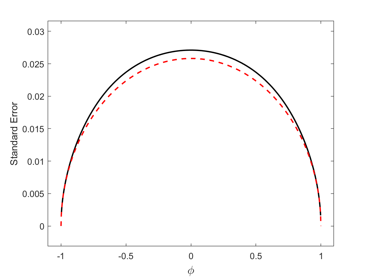
Figure 2: Set $T=250$. The black solid line denotes the standard error of $\hat{\phi}^{*}$ (or $\hat{\phi}^{ols}$). The red dashed line denotes the standard error of $\hat{\phi}^{\diamond}$.

4.3 Estimated Factors

We now provide a large-sample result for estimated factors:

$$\mathbb{E}_{\boldsymbol{f}_{t}|\boldsymbol{y}_{t},\hat{\boldsymbol{\theta}}^{*}}[\boldsymbol{f}_{t}]=[\hat{M}^{*,-1}+\hat{\Lambda}^{*,\intercal}\hat{\Sigma}_{ee}^{*,-1}\hat{\Lambda}^{*}]^{-1}\hat{\Lambda}^{*,\intercal}\hat{\Sigma}_{ee}^{*,-1}\boldsymbol{y}_{t},$$

for $t=1,\ldots,T$.

Theorem 2.

Suppose that the assumptions of Proposition 1 hold. If $\frac{N\cdot\log^{3}N}{T^{2}}\to 0$ as $N,T\to\infty$, we have

$$\sqrt{N}\left(\mathbb{E}_{\boldsymbol{f}_{t}|\boldsymbol{y}_{t},\hat{\boldsymbol{\theta}}^{*}}[\boldsymbol{f}_{t}]-\boldsymbol{f}_{t}\right)\xrightarrow{d}N(0,Q^{-1}),$$

where $Q\mathrel{\mathop{\mathchar 58\relax}}=\lim_{N\to\infty}\frac{1}{N}\Lambda^{\intercal}\Sigma_{ee}^{-1}\Lambda$.

Theorem 2 establishes the asymptotic distributions for the estimated factors. These asymptotic distributions are the same as Theorem 6.1(IC3) of Bai and Li (2012) and Proposition 5 of Barigozzi (2023) under the case of an exact factor model. As Barigozzi (2023) has pointed out, we need $N\to\infty$ to consistently estimate $\boldsymbol{f}_{t}$, as $\mathbb{E}_{\boldsymbol{f}_{t}|\boldsymbol{y}_{t},\hat{\boldsymbol{\theta}}^{*}}[\boldsymbol{f}_{t}]$ is some sort of cross-sectional average, and at the same time we need $T\to\infty$ to consistently estimate $\boldsymbol{f}_{t}$, as we use the QML-all-res estimators $\hat{\boldsymbol{\theta}}^{*}$, which are consistent only if $T\to\infty$. For both Theorems 1 and 2 holding, we need $CT^{1/2+\delta}\leq N\leq C^{\prime}T^{2-\delta}$ for some $0<\delta\leq 3/4$, which is in line with the discussion following Theorem 2 of Barigozzi and Luciani (2022). The asymptotic covariance matrix $Q^{-1}$ could be consistently estimated by $(\frac{1}{6N}\hat{\Lambda}^{*,\intercal}\hat{\Sigma}_{ee}^{*,-1}\hat{\Lambda}^{*})^{-1}$ (see (LABEL:f_r15) of the OS).

5 Monte Carlo Simulations

5.1 Baseline Simulations

In this section, we conduct Monte Carlo simulations to evaluate performance of QML-all-res. We specify $N=100,200$ and $T=250,750$, and a burn-in sample of 250 periods. Note that $T=250$ and $T=750$ correspond to two and six years’ daily data, respectively. Set $\phi=0.2$. For $c=\text{asia},\text{euro},\text{amer}$, the idiosyncratic variance $\sigma^{2}_{c,j}$ is drawn from uniform$[1,1.5]$ for $j=1,\ldots,N$, and

$$\beta_{c,j}=0.6a_{c,j}+0.4d_{c}-0.1,$$

$$\beta_{c,\text{a\_time},j}^{G}=0.6a_{c,\text{a\_time},j}+0.4d_{c,\text{a\_time}}-0.1,$$

$$\beta_{c,\text{e\_time},j}^{G}=0.6a_{c,\text{e\_time},j}+0.4d_{c,\text{e\_time}}-0.1,$$

$$\beta_{c,\text{am\_time},j}^{G}=0.6a_{c,\text{am\_time},j}+0.4d_{c,\text{am\_time}}-0.1,$$

where $\beta_{c,j},\beta_{c,\text{a\_time},j}^{G},\beta_{c,\text{e\_time},j}^{G},\beta_{c,\text{am\_time},j}^{G}$ are the $j$th component of $\boldsymbol{\beta}_{c}$, $\boldsymbol{\beta}_{c,\text{a\_time}}^{G}$, $\boldsymbol{\beta}_{c,\text{e\_time}}^{G}$, $\boldsymbol{\beta}_{c,\text{am\_time}}^{G}$, respectively, for $j=1,\ldots,N$, and $a_{c,j}$, $a_{c,\text{a\_time},j}$, $a_{c,\text{e\_time},j}$, $a_{c,\text{am\_time},j}$, $d_{c}$, $d_{c,\text{a\_time}}$, $d_{c,\text{e\_time}}$ and $d_{c,\text{am\_time}}$ are all drawn from uniform$[0,1]$. The econometrician observes those logarithmic 24-hour close-to-close returns. He is aware of the structure of the true model, but does not know the values of those parameters.

The number of the Monte Carlo samples is chosen to be 1000. From these 1000 Monte Carlo samples, we calculate the following three quantities for evaluation:

1. the root mean square error (RMSE) of the quantity of interest,

2. the average of the standard errors (Ave.se) of the estimated elements of the quantity of interest.

3. the average of the coverage probabilities (Cove) of the confidence intervals, formed by the point estimates $\pm$ 1.96$\times$the standard errors, of the elements of the quantity of interest.

Table 2 presents the RMSE, Ave.se, and Cove of the QML-all-res estimator. We see that the RMSE and Ave.se of the factor loadings are in general quite close to each other. However, in the case of $N=100$, the RMSE is slightly larger than the Ave.se, indicating that the standard errors are slightly underestimated when $N=100$. When $N$ increases to 200, the Ave.se gets closer to the RMSE. When $N$ increases from 100 to 200, the Cove improves considerably. We consider the size performance of QML-all-res pretty good as it is well known in the literature that size of large-dimensional factor models is difficult to control.

The performance of QML-all-res for $\Sigma_{ee}$ is very good, with the Cove being very close to 0.95. Obtaining a good estimate of $\Sigma_{ee}$ is relatively straightforward. In unreported Monte Carlo simulations, even the QML-just-identified estimator produces a reasonably accurate estimate of $\Sigma_{ee}$. When $N=100$, $T=250$ or 750, the standard error of $\hat{\phi}^{*}$ is under-estimated to some extent, resulting in a slightly lower Cove. However, the Cove improves as $N$ increases to 200.

	$N=100,T=250$				$N=100,T=750$
	RMSE	Ave.se	Cove		RMSE	Ave.se	Cove
$\boldsymbol{\beta}_{\text{asia,a\_time}}^{G}$	0.0634	0.0528	0.8943		0.0363	0.0306	0.8998
$\boldsymbol{\beta}_{\text{asia,am\_time}}^{G}$	0.0661	0.0555	0.8923		0.0376	0.0323	0.9002
$\boldsymbol{\beta}_{\text{asia,e\_time}}^{G}$	0.0683	0.0557	0.8842		0.0385	0.0323	0.8953
$\boldsymbol{\beta}_{\text{asia}}$	0.0575	0.0520	0.9224		0.0332	0.0303	0.9243
$\boldsymbol{\beta}_{\text{euro,e\_time}}^{G}$	0.0668	0.0520	0.8760		0.0381	0.0308	0.8830
$\boldsymbol{\beta}_{\text{euro,a\_time}}^{G}$	0.0716	0.0549	0.8588		0.0398	0.0314	0.8760
$\boldsymbol{\beta}_{\text{euro,am\_time}}^{G}$	0.0649	0.0530	0.8890		0.0372	0.0311	0.8949
$\boldsymbol{\beta}_{\text{euro}}$	0.0613	0.0538	0.9148		0.0349	0.0313	0.9230
$\boldsymbol{\beta}_{\text{amer,am\_time}}^{G}$	0.0631	0.0536	0.9002		0.0364	0.0306	0.9042
$\boldsymbol{\beta}_{\text{amer,e\_time}}^{G}$	0.0643	0.0544	0.8984		0.0370	0.0314	0.9017
$\boldsymbol{\beta}_{\text{amer,a\_time}}^{G}$	0.0632	0.0525	0.8943		0.0363	0.0304	0.8989
$\boldsymbol{\beta}_{\text{amer}}$	0.0614	0.0559	0.9187		0.0352	0.0319	0.9236
$\Sigma_{ee}$	0.0820	0.0792	0.9366		0.0471	0.0460	0.9418
$\phi$	0.0439	0.0276	0.8450		0.0213	0.0158	0.8750
	$N=200,T=250$				$N=200,T=750$
	RMSE	Ave.se	Cove		RMSE	Ave.se	Cove
$\boldsymbol{\beta}_{\text{asia,a\_time}}^{G}$	0.0552	0.0515	0.9301		0.0319	0.0298	0.9309
$\boldsymbol{\beta}_{\text{asia,am\_time}}^{G}$	0.0564	0.0537	0.9328		0.0323	0.0307	0.9353
$\boldsymbol{\beta}_{\text{asia,e\_time}}^{G}$	0.0555	0.0522	0.9339		0.0320	0.0303	0.9359
$\boldsymbol{\beta}_{\text{asia}}$	0.0558	0.0538	0.9402		0.0322	0.0313	0.9424
$\boldsymbol{\beta}_{\text{euro,e\_time}}^{G}$	0.0570	0.0505	0.9186		0.0327	0.0296	0.9222
$\boldsymbol{\beta}_{\text{euro,a\_time}}^{G}$	0.0580	0.0526	0.9207		0.0334	0.0304	0.9225
$\boldsymbol{\beta}_{\text{euro,am\_time}}^{G}$	0.0557	0.0510	0.9273		0.0321	0.0297	0.9303
$\boldsymbol{\beta}_{\text{euro}}$	0.0558	0.0531	0.9369		0.0321	0.0307	0.9396
$\boldsymbol{\beta}_{\text{amer,am\_time}}^{G}$	0.0587	0.0520	0.9137		0.0337	0.0303	0.9167
$\boldsymbol{\beta}_{\text{amer,e\_time}}^{G}$	0.0587	0.0529	0.9172		0.0339	0.0305	0.9177
$\boldsymbol{\beta}_{\text{amer,a\_time}}^{G}$	0.0585	0.0510	0.9109		0.0336	0.0294	0.9137
$\boldsymbol{\beta}_{\text{amer}}$	0.0564	0.0530	0.9319		0.0325	0.0305	0.9344
$\Sigma_{ee}$	0.0810	0.0791	0.9400		0.0466	0.0460	0.9445
$\phi$	0.0309	0.0272	0.9230		0.0176	0.0157	0.9200

Table 2: RMSE, Ave.se and Cove stand for the root mean square error of, average of the standard errors of the estimated elements of, and average of the coverage probabilities of the confidence intervals, formed by the point estimates $\pm$ 1.96$\times$the standard errors, of the elements of the quantity of interest, respectively.

In Figures 3 and 4, we present the QQ plots of the 10th element of the standardized QML-all-res of $\boldsymbol{\beta}^{G}_{\text{asia,a\_time}}$ and standardized $\hat{\phi}^{*}$, respectively, for illustrative purposes. The standardized estimator is calculated as the difference between the estimator and true value, divided by the standard error. These two plots demonstrate that our standardized estimators closely resemble the standard normal.

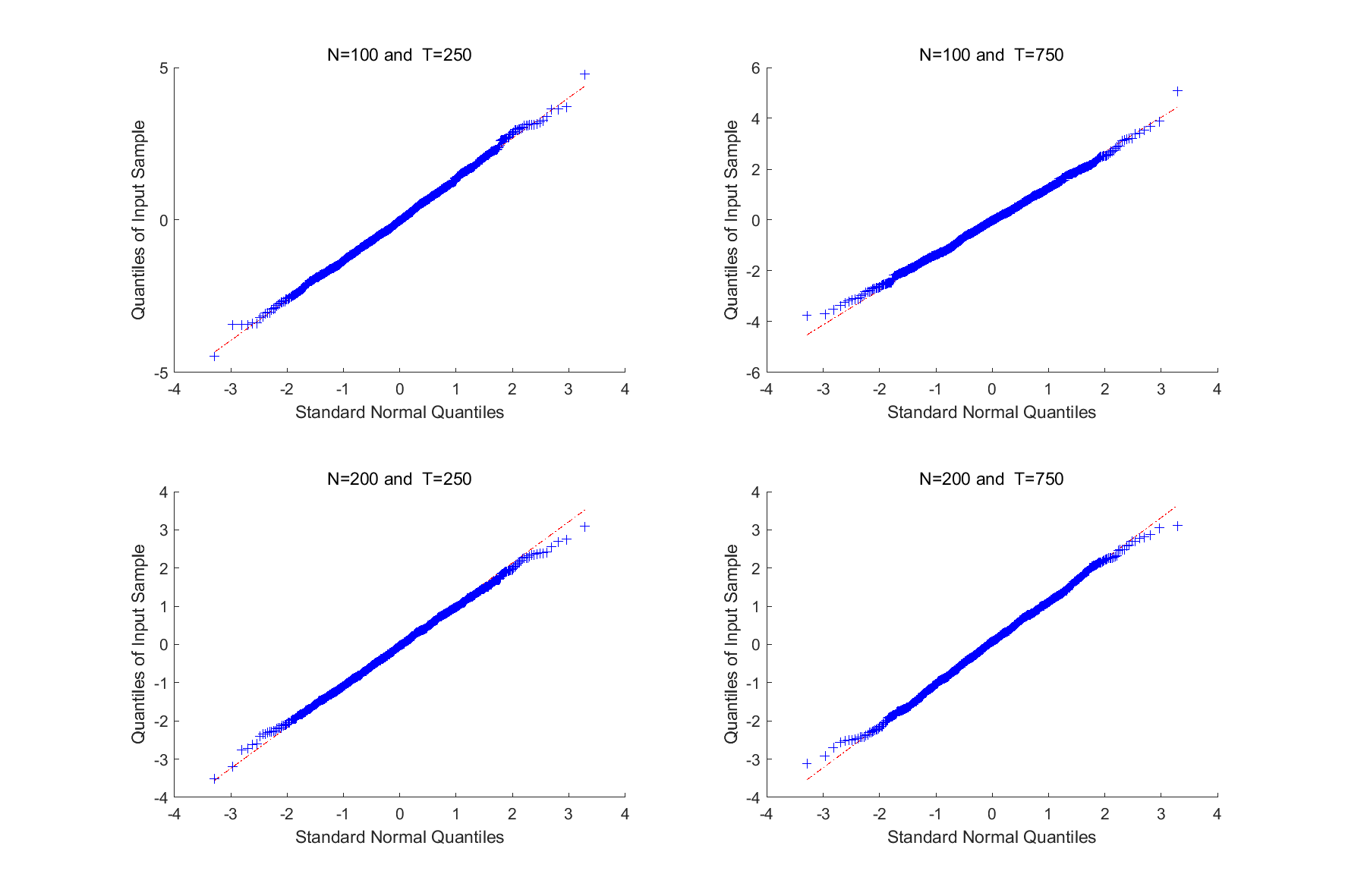
Figure 3: The 10th element of the standardized QML-all-res estimator of $\boldsymbol{\beta}^{G}_{\text{asia,a\_time}}$.

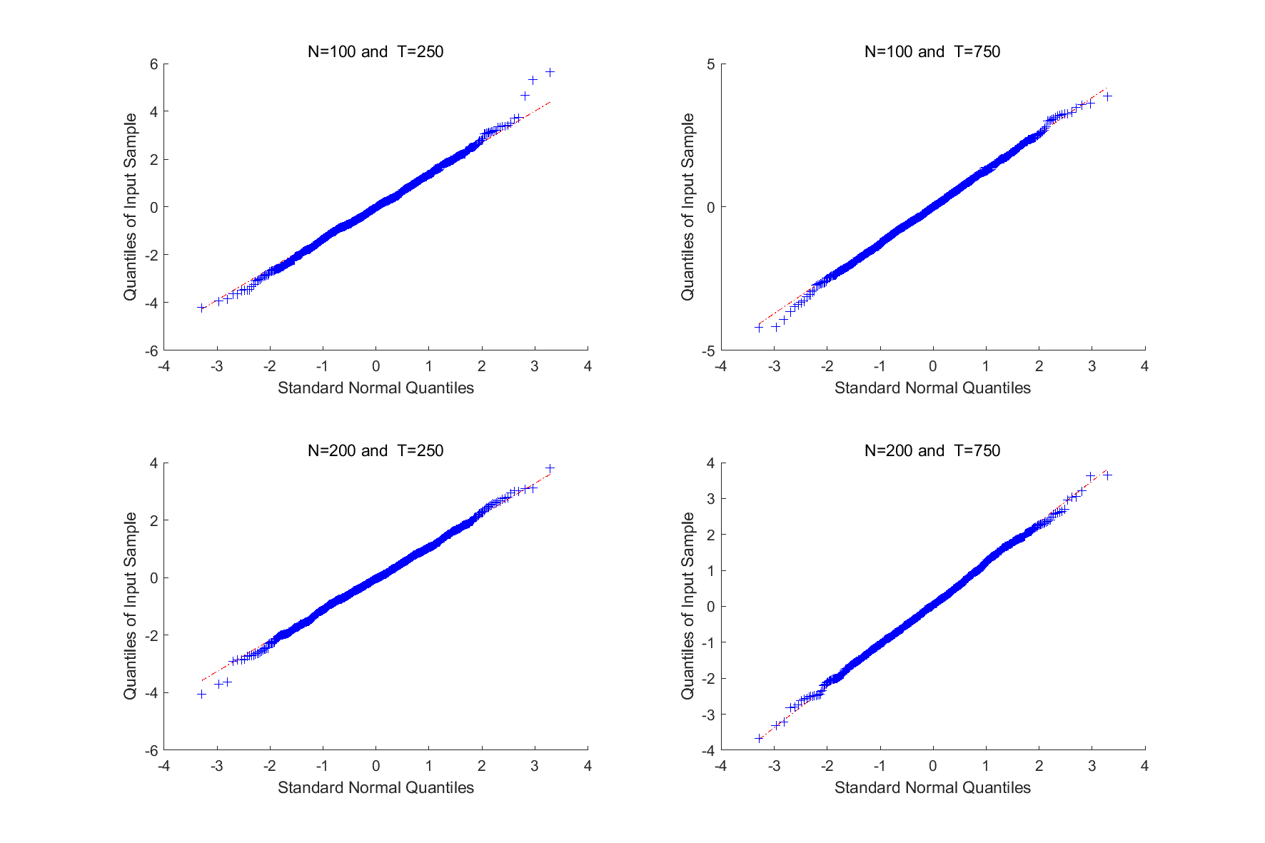
Figure 4: Standardized $\hat{\phi}^{*}$.

5.2 Simulations with Non-Gaussian Data

This section investigates simulations using data that deviate from the assumptions of the model. The parameters are generated in the same way as in Section 5.1. We draw each of $\eta_{s,\text{a\_time}}$, $\eta_{s,\text{e\_time}}$, $\eta_{s,\text{am\_time}}$, $f_{\text{asia},s}$, $f_{\text{euro},s}$, and $f_{\text{amer},s}$ independently across time from a $t$ distribution with 8 degrees of freedom and standardized to have variance 1. Furthermore, we include cross-correlation and auto-correlation in the idiosyncratic components. Specifically for $c=\text{asia},\text{euro},\text{amer}$, we generate $\boldsymbol{\epsilon}_{c,s}$ in the following way:

$$\boldsymbol{\epsilon}_{c,s} =b\boldsymbol{\epsilon}_{c,s-1}+C^{1/2}\boldsymbol{e}_{c,s}^{0}$$

where each of the elements in $\boldsymbol{e}_{c,s}^{0}$ is independently across time drawn from a $t$ distribution with 8 degrees of freedom and standardized to have variance 1, and $C$ is an $N\times N$ matrix which controls cross-correlation in the idiosyncratic components. We specify $C_{i,j}=\tau^{|i-j|}$ for $|i-j|\leq 10$, and 0 otherwise. We consider the following two cases:

Case 1: $\tau=0$ and $b=0$. In this case, we only consider non-normal data but switch off cross-correlation and auto-correlation in the idiosyncratic components.

Case 2: $\tau=0.3$ and $b=0.1$. In this case, we consider not only non-normal data but also cross-correlation and auto-correlation in the idiosyncratic components. We use a small $b$ because it is widely agreed that auto-correlation is quite small in finance.

The simulation results of these two cases are presented in Table 3. The performance of Case 1 or 2 is, as expected, worse than the baseline simulations, but still acceptable. The estimated standard errors become underestimated to some extent, a well known fact when fitting data generated from $t$ distributions using normal distributions. Take $\Sigma_{ee}$ (i.e., $\{\sigma_{k,j}^{2}\}$) as an example. The asymptotic variance of $\hat{\sigma}_{k,j}^{2,*}$ is a function of $\mathbb{E}[e_{t,k,j}^{4}]$. Under Gaussianity, $\mathbb{E}[e_{t,k,j}^{4}]=3\sigma_{k,j}^{4}$, so we can simplify the asymptotic variance to $\sigma_{k,j}^{4}$ as in (4.2). Under non-Gaussianity, $3\sigma_{k,j}^{4}$ underestimates $\mathbb{E}[e_{t,k,j}^{4}]$, so a straightforward solution is to use the sample 4th moment of $e_{t,k,j}$ to compute the standard error of $\hat{\sigma}_{k,j}^{2,*}$. Doing so indeed improves Ave.se and Cove (see the rows of $\Sigma_{ee}^{\dagger}$ in Table 3). We leave the theories covering non-normal data for future research. However, in the empirical application in Section 6, we observe that most estimates of the parameters are highly significant with $t$ statistics much larger than 2. Therefore, slight underestimation of the standard errors has little impact on drawing inference in our application.

Case 1	$N=200,T=250$				$N=200,T=750$
	RMSE	Ave.se	Cove		RMSE	Ave.se	Cove
$\boldsymbol{\beta}_{\text{asia,a\_time}}^{G}$	0.0563	0.0511	0.9244		0.0327	0.0297	0.9230
$\boldsymbol{\beta}_{\text{asia,am\_time}}^{G}$	0.0567	0.0538	0.9313		0.0327	0.0310	0.9331
$\boldsymbol{\beta}_{\text{asia,e\_time}}^{G}$	0.0561	0.0527	0.9307		0.0321	0.0304	0.9337
$\boldsymbol{\beta}_{\text{asia}}$	0.0565	0.0542	0.9367		0.0323	0.0313	0.9409
$\boldsymbol{\beta}_{\text{euro,e\_time}}^{G}$	0.0587	0.0515	0.9093		0.0339	0.0294	0.9105
$\boldsymbol{\beta}_{\text{euro,a\_time}}^{G}$	0.0581	0.0526	0.9197		0.0339	0.0303	0.9180
$\boldsymbol{\beta}_{\text{euro,am\_time}}^{G}$	0.0567	0.0511	0.9227		0.0328	0.0299	0.9237
$\boldsymbol{\beta}_{\text{euro}}$	0.0564	0.0530	0.9337		0.0323	0.0308	0.9384
$\boldsymbol{\beta}_{\text{amer,am\_time}}^{G}$	0.0603	0.0507	0.9041		0.0350	0.0302	0.9042
$\boldsymbol{\beta}_{\text{amer,e\_time}}^{G}$	0.0603	0.0534	0.9088		0.0344	0.0303	0.9144
$\boldsymbol{\beta}_{\text{amer,a\_time}}^{G}$	0.0595	0.0511	0.9050		0.0345	0.0296	0.9048
$\boldsymbol{\beta}_{\text{amer}}$	0.0575	0.0532	0.9256		0.0330	0.0307	0.9298
$\Sigma_{ee}$	0.1058	0.0794	0.8547		0.0613	0.0461	0.8568
$\Sigma_{ee}^{\dagger}$	0.1058	0.1011	0.9206		0.0613	0.0592	0.9331
$\phi$	0.0306	0.0272	0.9070		0.0178	0.0157	0.9150
Case 2	$N=200,T=250$				$N=200,T=750$
	RMSE	Ave.se	Cove		RMSE	Ave.se	Cove
$\boldsymbol{\beta}_{\text{asia,a\_time}}^{G}$	0.0572	0.0510	0.9184		0.0336	0.0297	0.9147
$\boldsymbol{\beta}_{\text{asia,am\_time}}^{G}$	0.0581	0.0537	0.9233		0.0339	0.0309	0.9224
$\boldsymbol{\beta}_{\text{asia,e\_time}}^{G}$	0.0580	0.0524	0.9205		0.0338	0.0303	0.9187
$\boldsymbol{\beta}_{\text{asia}}$	0.0606	0.0540	0.9160		0.0364	0.0312	0.9038
$\boldsymbol{\beta}_{\text{euro,e\_time}}^{G}$	0.0599	0.0516	0.9030		0.0349	0.0294	0.8999
$\boldsymbol{\beta}_{\text{euro,a\_time}}^{G}$	0.0593	0.0522	0.9119		0.0347	0.0302	0.9094
$\boldsymbol{\beta}_{\text{euro,am\_time}}^{G}$	0.0581	0.0515	0.9150		0.0339	0.0299	0.9140
$\boldsymbol{\beta}_{\text{euro}}$	0.0600	0.0529	0.9145		0.0357	0.0308	0.9071
$\boldsymbol{\beta}_{\text{amer,am\_time}}^{G}$	0.0620	0.0502	0.8944		0.0364	0.0302	0.8907
$\boldsymbol{\beta}_{\text{amer,e\_time}}^{G}$	0.0615	0.0529	0.9014		0.0355	0.0302	0.9020
$\boldsymbol{\beta}_{\text{amer,a\_time}}^{G}$	0.0606	0.0508	0.8986		0.0352	0.0295	0.8969
$\boldsymbol{\beta}_{\text{amer}}$	0.0604	0.0530	0.9104		0.0359	0.0306	0.9034
$\Sigma_{ee}$	0.1049	0.0790	0.8551		0.0611	0.0460	0.8559
$\Sigma_{ee}^{\dagger}$	0.1049	0.0986	0.9154		0.0611	0.0577	0.9265
$\phi$	0.0347	0.0273	0.8830		0.0198	0.0157	0.8780

Table 3: Case 1: non-normal data. Case 2: non-normal data with cross-correlated and auto-correlated idiosyncratic components. The standard errors in rows of $\Sigma_{ee}^{\dagger}$ are computed using the sample 4th moment of $e_{t,k,j}$. RMSE, Ave.se and Cove stand for the root mean square error of, average of the standard errors of the estimated elements of, and average of the coverage probabilities of the confidence intervals, formed by the point estimates $\pm$ 1.96$\times$the standard errors, of the elements of the quantity of interest, respectively.

In Figures 5 and 6, we present the QQ plots of the 10th element of the standardized QML-all-res of $\boldsymbol{\beta}^{G}_{\text{asia,a\_time}}$ and standardized $\hat{\phi}^{*}$, respectively, for illustrative purposes. The standardized estimator is calculated as the difference between the estimator and true value, divided by the standard error. These two plots demonstrate that our standardized estimators closely resemble the standard normal.

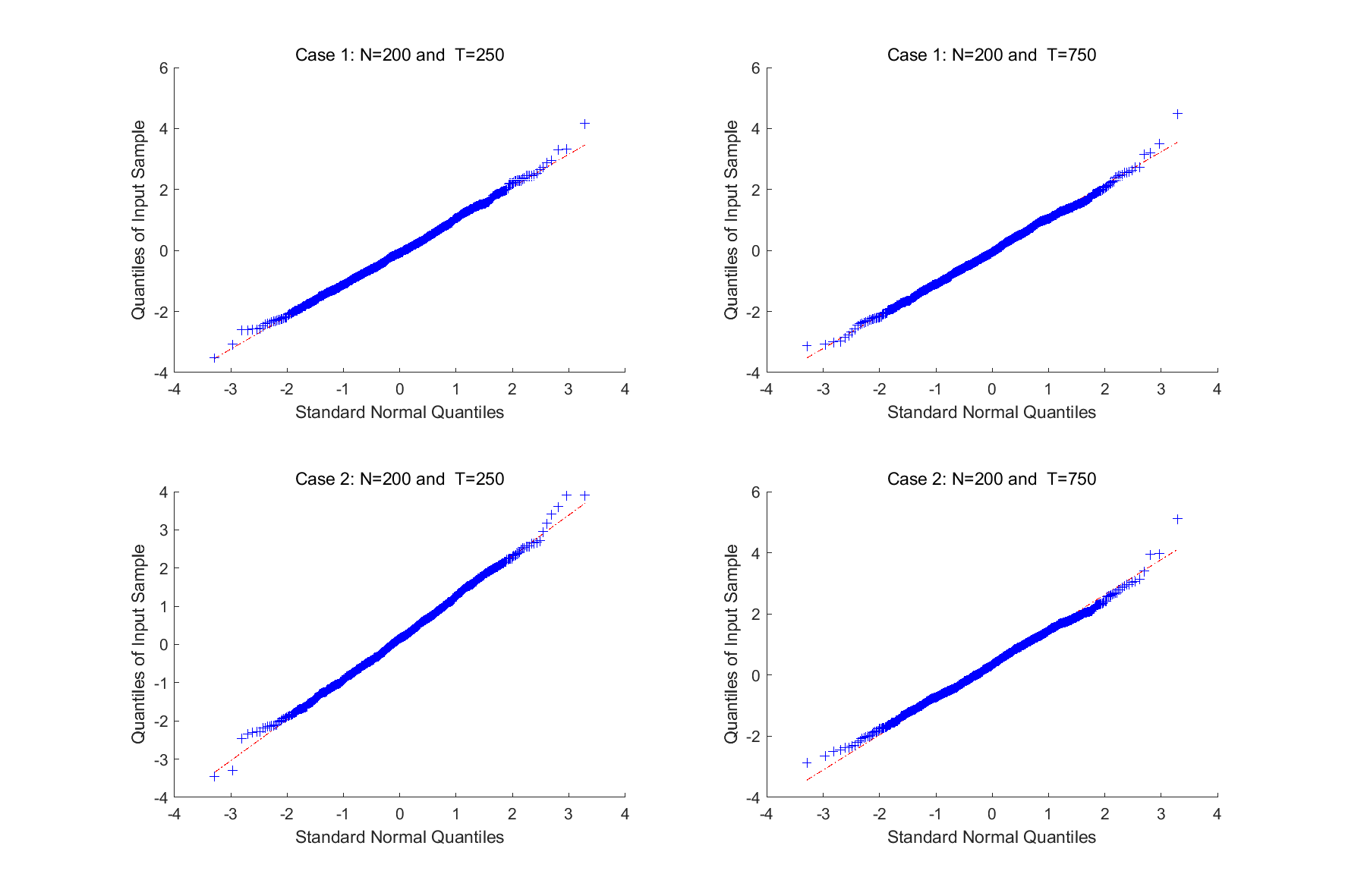
Figure 5: The 10th element of the standardized QML-all-res estimator of $\boldsymbol{\beta}^{G}_{\text{asia,a\_time}}$.

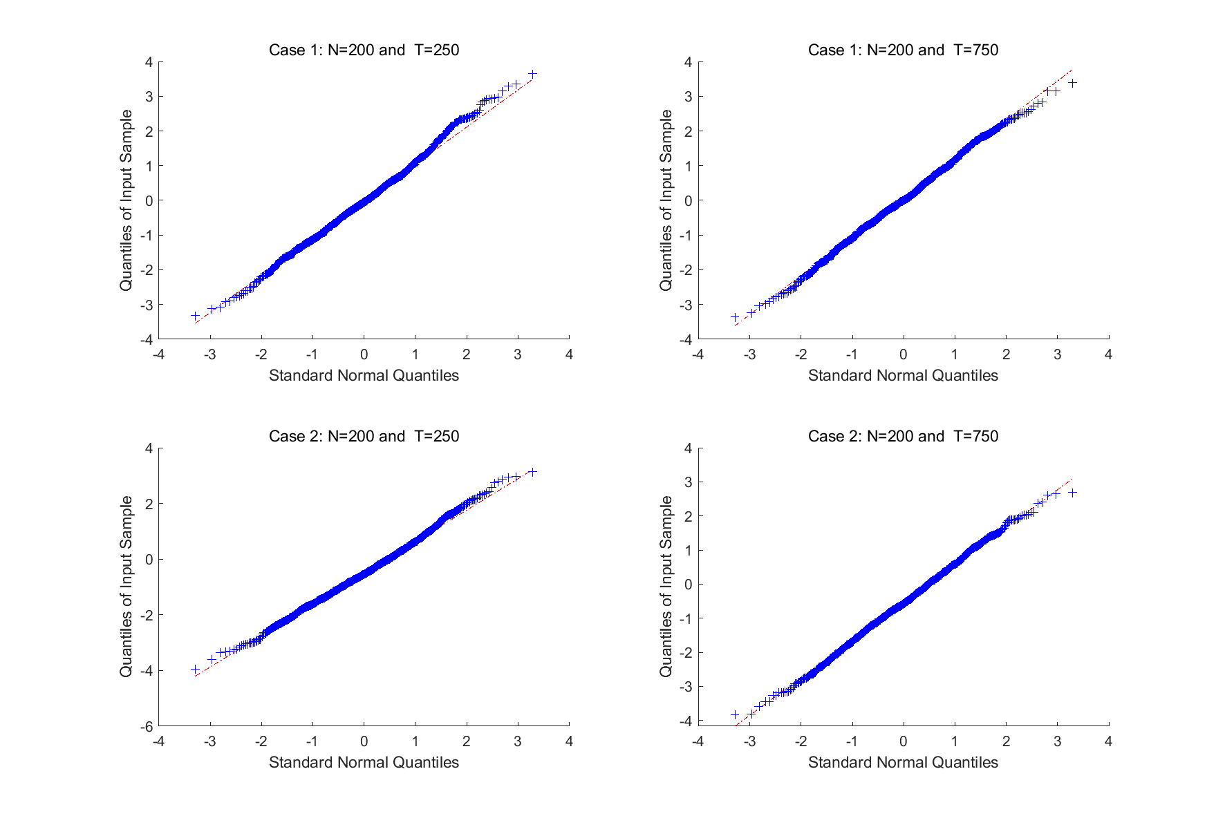
Figure 6: Standardized $\hat{\phi}^{*}$.

6 Empirical Application

We apply our model to MSCI equity indices of 42 developed and emerging markets. Daily indices were obtained from Eikon. The data are from May 5th, 2014 (the date when most indices are available) to June 23rd, 2023. For most markets, there are 6 indices (in USD currency): Large-Growth, Mid-Growth, Small-Growth, Large-Value, Mid-Value, and Small-Value. We have 212 indices in total. Dates with more than 50 missing indices are excluded.

We categorize these markets into three continents based on their closing times: Asia-Pacific, Europe, and Americas. We exclude the Israeli market from our sample because its closing time is far away from those of Asia-Pacific or Europe. All the returns have been demeaned. To better compare magnitudes of the loadings, we also standardize the returns so that they have unit variances (Stock and Watson (2016, p.422)). We shall use QML-all-res.

6.1 Basic Results

Table 4 displays the estimated factor loadings and idiosyncratic variances for Asia-Pacific. The indices for Mainland China, Hong Kong, and Japan are all presented, while only the Mid-Value and Mid-Growth indices are shown for other Asia-Pacific markets in the interest of space. Recall that $\boldsymbol{\beta}_{\text{asia, a\_time}}^{G}$ represents the loading of the global factor during the Asian sub-period (from the American close on day $s-1$ to the Asian close on day $s$), and likewise for others. We have made two main observations. First, for the Asia-Pacific markets, the global factor has the largest loadings during the Asian sub-period, with Australia having the largest ones at approximately 0.7. Second, Mainland China and Hong Kong have large loadings of the continental factor, around 0.7, whereas Japan has minimal loadings of the continental factor.

	$\boldsymbol{\beta}_{\text{asia,a\_time},i}^{G}$	$\boldsymbol{\beta}_{\text{asia,am\_time},i}^{G}$	$\boldsymbol{\beta}_{\text{asia,e\_time},i}^{G}$	$\boldsymbol{\beta}_{\text{asia},i}$	$\sigma^{2}_{\text{asia},i}$
Mainland China LG	0.385 (0.011)	0.053 (0.011)	-0.144 (0.011)	0.719 (0.011)	0.295 (0.014)
Mainland China LV	0.429 (0.009)	0.132 (0.009)	-0.031 (0.009)	0.754 (0.010)	0.211 (0.010)
Mainland China MG	0.371 (0.011)	0.065 (0.011)	-0.142 (0.011)	0.734 (0.011)	0.284 (0.013)
Mainland China MV	0.386 (0.008)	0.106 (0.008)	-0.086 (0.008)	0.823 (0.008)	0.142 (0.007)
Mainland China SG	0.338 (0.009)	0.087 (0.009)	-0.159 (0.008)	0.816 (0.009)	0.173 (0.008)
Mainland China SV	0.364 (0.008)	0.113 (0.008)	-0.089 (0.008)	0.819 (0.008)	0.162 (0.008)
Hong Kong LG	0.399 (0.012)	0.136 (0.012)	0.001 (0.012)	0.673 (0.012)	0.351 (0.017)
Hong Kong LV	0.433 (0.014)	0.136 (0.014)	0.140 (0.014)	0.536 (0.014)	0.457 (0.022)
Hong Kong MG	0.393 (0.015)	0.078 (0.015)	-0.071 (0.015)	0.518 (0.016)	0.554 (0.026)
Hong Kong MV	0.432 (0.013)	0.128 (0.013)	0.079 (0.013)	0.607 (0.013)	0.400 (0.019)
Hong Kong SG	0.377 (0.009)	0.150 (0.009)	-0.094 (0.009)	0.780 (0.010)	0.204 (0.010)
Hong Kong SV	0.402 (0.011)	0.168 (0.011)	0.013 (0.010)	0.726 (0.011)	0.260 (0.012)
Japan LG	0.343 (0.014)	0.604 (0.014)	-0.155 (0.013)	0.116 (0.014)	0.429 (0.020)
Japan LV	0.328 (0.014)	0.574 (0.014)	-0.072 (0.014)	0.061 (0.015)	0.483 (0.023)
Japan MG	0.340 (0.014)	0.598 (0.014)	-0.162 (0.014)	0.105 (0.014)	0.443 (0.021)
Japan MV	0.339 (0.014)	0.578 (0.014)	-0.064 (0.014)	0.058 (0.014)	0.467 (0.022)
Japan SG	0.334 (0.014)	0.594 (0.014)	-0.162 (0.014)	0.095 (0.014)	0.456 (0.022)
Japan SV	0.326 (0.014)	0.583 (0.014)	-0.085 (0.014)	0.043 (0.015)	0.476 (0.022)
South Korea MV	0.500 (0.014)	0.239 (0.014)	0.248 (0.013)	0.344 (0.014)	0.432 (0.020)
Taiwan MV	0.432 (0.014)	0.263 (0.014)	0.182 (0.014)	0.388 (0.015)	0.490 (0.023)
Australia MV	0.724 (0.012)	0.275 (0.012)	-0.010 (0.012)	0.037 (0.012)	0.336 (0.016)
India MV	0.517 (0.016)	-0.038 (0.016)	0.259 (0.016)	0.207 (0.017)	0.625 (0.029)
Indonesia MV	0.438 (0.016)	0.017 (0.016)	0.341 (0.016)	0.199 (0.017)	0.632 (0.030)
Malaysia MV	0.478 (0.016)	0.068 (0.015)	0.331 (0.015)	0.241 (0.016)	0.564 (0.027)
New Zealand MV	0.519 (0.017)	0.192 (0.017)	-0.013 (0.017)	-0.019 (0.017)	0.663 (0.031)
Philippines MV	0.341 (0.018)	0.081 (0.018)	0.277 (0.017)	0.210 (0.018)	0.724 (0.034)
Singapore MV	0.642 (0.014)	0.138 (0.014)	0.169 (0.014)	0.239 (0.014)	0.441 (0.021)
Thailand MV	0.521 (0.016)	-0.001 (0.016)	0.247 (0.016)	0.219 (0.016)	0.613 (0.029)
South Korea MG	0.477 (0.014)	0.251 (0.014)	0.182 (0.014)	0.362 (0.015)	0.476 (0.022)
Taiwan MG	0.412 (0.015)	0.263 (0.015)	0.105 (0.015)	0.375 (0.016)	0.555 (0.026)
Australia MG	0.729 (0.011)	0.318 (0.011)	-0.113 (0.011)	0.063 (0.011)	0.290 (0.014)
India MG	0.512 (0.016)	-0.004 (0.016)	0.233 (0.016)	0.221 (0.017)	0.629 (0.030)
Indonesia MG	0.412 (0.017)	0.001 (0.017)	0.358 (0.016)	0.187 (0.017)	0.650 (0.031)
Malaysia MG	0.371 (0.017)	0.094 (0.017)	0.218 (0.017)	0.270 (0.018)	0.705 (0.033)
New Zealand MG	0.378 (0.018)	0.213 (0.018)	-0.090 (0.018)	0.023 (0.019)	0.784 (0.037)
Philippines MG	0.299 (0.018)	0.080 (0.018)	0.275 (0.018)	0.164 (0.018)	0.770 (0.036)
Singapore MG	0.638 (0.014)	0.132 (0.014)	0.160 (0.013)	0.272 (0.014)	0.436 (0.021)
Thailand MG	0.482 (0.017)	-0.021 (0.017)	0.219 (0.017)	0.202 (0.017)	0.678 (0.032)

Table 4: Selected QML-all-res estimates of the factor loadings and idiosyncratic variances. LG, LV, MG, MV, SG, SV, stand for Large-Growth, Large-Value, Mid-Growth, Mid-Value, Small-Growth and Small-Value, respectively. The standard errors are in parentheses.

Table 5 displays the estimated factor loadings and idiosyncratic variances for the Europe. All the indices of the UK, France, and Germany are reported, while only the Mid-Value and Mid-Growth indices are reported for other European markets to save space. We have identified three key findings. First, all the European markets have substantial loadings of the global factor during the Asian sub-period, but small loadings of the global factor during the American sub-period. Second, all the Value indices exhibit non-negative loadings of the global factor during the European sub-period, particularly for the Large-Value ones. Conversely, most Growth indices have negative loadings of the global factor during the European sub-period. Third, most European markets have considerably large loadings of the continental factor, except for South Africa and Turkey.

	$\boldsymbol{\beta}_{\text{euro,e\_time},i}^{G}$	$\boldsymbol{\beta}_{\text{euro,a\_time},i}^{G}$	$\boldsymbol{\beta}_{\text{euro,am\_time},i}^{G}$	$\boldsymbol{\beta}_{\text{euro},i}$	$\sigma^{2}_{\text{euro},i}$
United Kingdom LG	-0.025 (0.016)	0.605 (0.013)	0.065 (0.012)	0.512 (0.013)	0.358 (0.017)
United Kingdom LV	0.402 (0.012)	0.534 (0.010)	0.057 (0.009)	0.472 (0.010)	0.209 (0.010)
United Kingdom MG	-0.081 (0.012)	0.688 (0.010)	0.058 (0.009)	0.577 (0.009)	0.201 (0.009)
United Kingdom MV	0.131 (0.013)	0.606 (0.011)	0.092 (0.009)	0.550 (0.010)	0.233 (0.011)
United Kingdom SG	-0.082 (0.013)	0.672 (0.011)	0.091 (0.010)	0.553 (0.010)	0.239 (0.011)
United Kingdom SV	0.157 (0.013)	0.603 (0.011)	0.111 (0.010)	0.526 (0.010)	0.242 (0.011)
France LG	-0.076 (0.011)	0.628 (0.009)	0.021 (0.008)	0.665 (0.009)	0.175 (0.008)
France LV	0.382 (0.008)	0.469 (0.007)	0.065 (0.006)	0.664 (0.006)	0.094 (0.004)
France MG	-0.085 (0.010)	0.646 (0.008)	0.059 (0.007)	0.675 (0.008)	0.134 (0.006)
France MV	0.263 (0.010)	0.522 (0.009)	0.079 (0.007)	0.646 (0.008)	0.145 (0.007)
France SG	-0.200 (0.010)	0.674 (0.009)	0.041 (0.008)	0.657 (0.008)	0.153 (0.007)
France SV	0.177 (0.010)	0.581 (0.008)	0.089 (0.007)	0.633 (0.008)	0.141 (0.007)
Germany LG	-0.148 (0.011)	0.632 (0.009)	0.017 (0.008)	0.680 (0.009)	0.169 (0.008)
Germany LV	0.211 (0.009)	0.520 (0.008)	0.053 (0.007)	0.694 (0.007)	0.124 (0.006)
Germany MG	-0.326 (0.010)	0.713 (0.009)	-0.008 (0.007)	0.642 (0.008)	0.143 (0.007)
Germany MV	0.085 (0.012)	0.565 (0.010)	0.030 (0.009)	0.642 (0.010)	0.217 (0.010)
Germany SG	-0.297 (0.010)	0.703 (0.008)	0.022 (0.007)	0.658 (0.008)	0.129 (0.006)
Germany SV	0.024 (0.009)	0.659 (0.008)	0.047 (0.007)	0.640 (0.007)	0.123 (0.006)
Austria MV	0.376 (0.016)	0.424 (0.013)	0.043 (0.011)	0.512 (0.012)	0.335 (0.016)
Belgium MV	0.213 (0.016)	0.428 (0.013)	0.056 (0.011)	0.608 (0.012)	0.339 (0.016)
Denmark MV	0.148 (0.022)	0.355 (0.018)	0.102 (0.016)	0.370 (0.017)	0.664 (0.031)
Finland MV	0.047 (0.017)	0.543 (0.014)	0.024 (0.012)	0.525 (0.013)	0.398 (0.019)
Greece MV	0.164 (0.023)	0.284 (0.020)	0.074 (0.017)	0.314 (0.018)	0.758 (0.036)
Italy MV	0.318 (0.013)	0.377 (0.011)	0.019 (0.009)	0.679 (0.010)	0.234 (0.011)
Netherlands MV	0.328 (0.012)	0.465 (0.010)	0.067 (0.009)	0.611 (0.010)	0.212 (0.010)
Norway MV	0.121 (0.019)	0.582 (0.016)	0.014 (0.014)	0.327 (0.015)	0.483 (0.023)
Poland MV	0.136 (0.021)	0.453 (0.018)	0.072 (0.015)	0.330 (0.016)	0.613 (0.029)
SouthAfrica MV	0.173 (0.016)	0.704 (0.014)	-0.060 (0.012)	0.130 (0.013)	0.363 (0.017)
Spain MV	0.396 (0.014)	0.413 (0.012)	0.064 (0.011)	0.547 (0.011)	0.289 (0.014)
Sweden MV	-0.022 (0.013)	0.653 (0.011)	0.004 (0.010)	0.563 (0.011)	0.251 (0.012)
Switzerland MV	0.148 (0.013)	0.585 (0.011)	0.077 (0.009)	0.581 (0.010)	0.220 (0.010)
Turkey MV	0.123 (0.024)	0.351 (0.020)	-0.053 (0.018)	0.122 (0.019)	0.815 (0.038)
Belgium MG	-0.203 (0.018)	0.564 (0.015)	0.022 (0.013)	0.531 (0.014)	0.434 (0.020)
Denmark MG	-0.412 (0.016)	0.672 (0.013)	0.029 (0.012)	0.490 (0.012)	0.350 (0.016)
Finland MG	-0.114 (0.019)	0.498 (0.016)	0.007 (0.014)	0.508 (0.015)	0.513 (0.024)
Ireland MG	-0.243 (0.021)	0.470 (0.017)	0.024 (0.015)	0.455 (0.016)	0.595 (0.028)
Italy MG	0.011 (0.014)	0.480 (0.012)	-0.000 (0.010)	0.694 (0.011)	0.277 (0.013)
Netherlands MG	-0.351 (0.017)	0.601 (0.014)	0.022 (0.012)	0.540 (0.013)	0.383 (0.018)
Norway MG	-0.036 (0.020)	0.583 (0.016)	0.012 (0.014)	0.354 (0.015)	0.535 (0.025)
Poland MG	-0.020 (0.019)	0.562 (0.016)	0.025 (0.014)	0.388 (0.015)	0.526 (0.025)
Portugal MG	0.072 (0.022)	0.366 (0.018)	0.041 (0.016)	0.413 (0.017)	0.666 (0.031)
SouthAfrica MG	0.042 (0.018)	0.682 (0.016)	-0.063 (0.014)	0.152 (0.014)	0.475 (0.022)
Spain MG	-0.116 (0.022)	0.353 (0.019)	0.028 (0.016)	0.430 (0.018)	0.702 (0.033)
Sweden MG	-0.256 (0.012)	0.731 (0.010)	-0.011 (0.009)	0.562 (0.010)	0.211 (0.010)
Switzerland MG	-0.415 (0.012)	0.735 (0.010)	0.032 (0.009)	0.545 (0.010)	0.217 (0.010)
Turkey MG	0.089 (0.024)	0.374 (0.020)	-0.053 (0.018)	0.142 (0.019)	0.805 (0.038)

Table 5: Selected QML-all-res estimates of the factor loadings and idiosyncratic variances. LG, LV, MG, MV, SG, SV, stand for Large-Growth, Large-Value, Mid-Growth, Mid-Value, Small-Growth and Small-Value, respectively. The standard errors are in parentheses.

Table 6 presents the estimated factor loadings and idiosyncratic variances for Americas. We see that the United States and Canada have substantial loadings of the global factor during the American sub-period, whereas their loadings of the continental factor are negligible. On the other hand, the emerging American markets tend to have significantly large loadings of the global factor during the Asian sub-period. Brazil also has large loadings of the continental factor.

	$\boldsymbol{\beta}_{\text{amer,am\_time},i}^{G}$	$\boldsymbol{\beta}_{\text{amer,e\_time},i}^{G}$	$\boldsymbol{\beta}_{\text{amer,a\_time},i}^{G}$	$\boldsymbol{\beta}_{\text{amer},i}$	$\sigma^{2}_{\text{amer},i}$
United States LG	1.013 (0.012)	-0.346 (0.012)	0.332 (0.010)	0.098 (0.009)	0.188 (0.009)
United States LV	0.993 (0.010)	0.093 (0.010)	0.276 (0.008)	0.060 (0.008)	0.133 (0.006)
United States MG	1.069 (0.008)	-0.334 (0.008)	0.354 (0.007)	0.083 (0.006)	0.095 (0.005)
United States MV	1.020 (0.007)	0.090 (0.007)	0.301 (0.006)	0.064 (0.006)	0.072 (0.003)
United States SG	1.089 (0.007)	-0.204 (0.008)	0.320 (0.006)	0.074 (0.006)	0.078 (0.004)
United States SV	1.014 (0.008)	0.130 (0.008)	0.267 (0.007)	0.055 (0.006)	0.089 (0.004)
Brazil LG	0.271 (0.008)	0.145 (0.008)	0.413 (0.007)	0.758 (0.007)	0.097 (0.005)
Brazil LV	0.240 (0.011)	0.281 (0.012)	0.376 (0.010)	0.672 (0.009)	0.185 (0.009)
Brazil MG	0.264 (0.007)	0.125 (0.007)	0.423 (0.006)	0.779 (0.006)	0.069 (0.003)
Brazil MV	0.248 (0.009)	0.200 (0.009)	0.405 (0.007)	0.741 (0.007)	0.109 (0.005)
Brazil SG	0.269 (0.008)	0.127 (0.008)	0.413 (0.006)	0.777 (0.006)	0.080 (0.004)
Brazil SV	0.233 (0.006)	0.172 (0.006)	0.414 (0.005)	0.788 (0.005)	0.053 (0.003)
Canada LG	0.691 (0.015)	-0.128 (0.015)	0.559 (0.012)	0.068 (0.011)	0.298 (0.014)
Canada LV	0.590 (0.013)	0.228 (0.013)	0.520 (0.011)	0.054 (0.010)	0.233 (0.011)
Canada MG	0.643 (0.014)	-0.104 (0.014)	0.608 (0.012)	0.072 (0.011)	0.272 (0.013)
Canada MV	0.512 (0.015)	0.123 (0.015)	0.572 (0.013)	0.057 (0.012)	0.316 (0.015)
Canada SG	0.569 (0.016)	-0.115 (0.016)	0.602 (0.013)	0.066 (0.013)	0.356 (0.017)
Canada SV	0.518 (0.015)	0.091 (0.015)	0.596 (0.012)	0.057 (0.011)	0.299 (0.014)
Chile LG	0.289 (0.021)	0.041 (0.021)	0.503 (0.017)	0.143 (0.016)	0.598 (0.028)
Chile LV	0.198 (0.021)	0.160 (0.021)	0.476 (0.018)	0.147 (0.016)	0.607 (0.029)
Chile MG	0.157 (0.022)	0.073 (0.023)	0.446 (0.019)	0.115 (0.018)	0.713 (0.034)
Chile MV	0.157 (0.022)	0.148 (0.022)	0.440 (0.019)	0.133 (0.017)	0.676 (0.032)
Chile SG	0.154 (0.022)	0.109 (0.022)	0.485 (0.018)	0.101 (0.017)	0.656 (0.031)
Chile SV	0.169 (0.021)	0.104 (0.021)	0.500 (0.018)	0.104 (0.017)	0.636 (0.030)
Colombia LG	0.321 (0.021)	0.197 (0.021)	0.393 (0.018)	0.159 (0.016)	0.606 (0.029)
Colombia LV	0.324 (0.019)	0.228 (0.020)	0.438 (0.016)	0.173 (0.015)	0.529 (0.025)
Colombia SV	0.190 (0.023)	0.156 (0.023)	0.373 (0.019)	0.130 (0.018)	0.726 (0.034)
Mexico LG	0.305 (0.019)	0.154 (0.020)	0.489 (0.016)	0.180 (0.015)	0.528 (0.025)
Mexico LV	0.299 (0.019)	0.127 (0.019)	0.533 (0.016)	0.168 (0.015)	0.499 (0.024)
Mexico MG	0.253 (0.020)	0.017 (0.020)	0.554 (0.017)	0.136 (0.016)	0.569 (0.027)
Mexico MV	0.260 (0.019)	0.123 (0.019)	0.555 (0.016)	0.152 (0.015)	0.501 (0.024)
Mexico SG	0.298 (0.019)	0.087 (0.019)	0.556 (0.016)	0.164 (0.015)	0.495 (0.023)
Mexico SV	0.293 (0.019)	0.094 (0.019)	0.546 (0.016)	0.167 (0.015)	0.507 (0.024)
Peru LG	0.522 (0.020)	0.111 (0.020)	0.372 (0.017)	0.114 (0.016)	0.549 (0.026)

Table 6: Selected QML-all-res estimates of the factor loadings and idiosyncratic variances. LG, LV, MG, MV, SG, SV, stand for Large-Growth, Large-Value, Mid-Growth, Mid-Value, Small-Growth and Small-Value, respectively. The standard errors are in parentheses.

Overall, a large number of developing countries have large loadings of the global factor during the Asian sub-period. This means that the international news happened during the period between the American close on day $s-1$ and the Asian close on day $s$ has a substantial impact on the stock returns of these developing countries. Table 7 presents $\hat{\phi}^{*}=0.2491$ which is significantly different from 0. This implies that the weak-form efficient market hypothesis does not hold and it takes more than a $1/3$ day for some international news to fully unfold or dissipate. Figure 7 plots the estimated factors. We see that the global factor had a very large negative shock during the March of 2020, a period where the global stock markets crashed in the fear of Covid-19.

	Estimated value	Standard error
$\phi$	0.2491	0.0125

Table 7: The QML-all-res estimate of $\phi$, measuring the autocorrelation of the global factor.

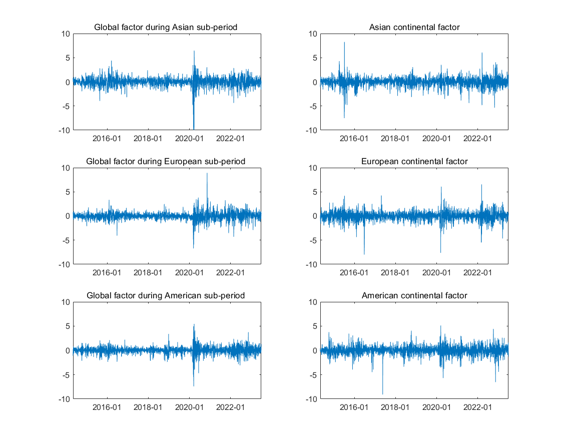
Figure 7: The estimated factors.

6.2 Integration

Financial market integration holds significant importance in the field of international finance. In our investigation, we adopt a methodology similar to Pukthuanthong and Roll (2009) to assess market integration. Pukthuanthong and Roll (2009) used the R-squared as a measure of integration, which is the proportion of variance explained by the explanatory variables. We define the proportion of variance explained by the global factor as the global integration index, while that explained by the continental factor as the regional integration index. The non-integration index is calculated as: $1-\text{global integration index}-\text{regional integration index}$.

Table 8 presents an analysis of integration of Asia-Pacific. We find that Mainland China and Hong Kong play a significant role in driving the Asia-Pacific regional integration. Specifically, most these markets demonstrate high regional integration, with approximately 50% of their variances explained by the continental factor. On the contrary, Japan shows high global integration, with over 50% of its variance explained by the global factor, but displays very low regional integration. In other words, Japanese indices are more globally integrated, while Chinese indices are more regionally integrated.

Table 9 presents an analysis of integration of Europe. The developed European markets, such as the UK, France, and Germany, exhibit higher levels of both the global and regional integration. On the other hand, the less developed European markets, such as Greece, Portugal, and Turkey, show lower levels of integration. For instance, the non-integration index of Turkish Mid-Growth index is as high as 81.19%, indicating that 81.19% of the variance of the Turkish Mid-Growth index is explained by neither the global nor continental factor.

Table 10 presents an analysis of integration of Americas. The US market demonstrates the highest level of global integration, with the global factor accounting for approximately 90% of its variance. However, the US market lacks regional integration, meaning it is not influenced by the American continental factor. Within Americas, Brazil holds the most prominent role in regional integration.

In summary, the US market is largely globally integrated, with approximately 90% of the variance of its returns being explained by the global factor. The Asia-Pacific regional integration is primarily driven by Mainland China and Hong Kong, while the American regional integration is mainly driven by Brazil. The developed and emerging markets exhibit different patterns.

	Global integration	Regional integration	Non-integration
Mainland China LG	0.1838	0.5192	0.2970
Mainland China LV	0.2365	0.5566	0.2069
Mainland China MG	0.1738	0.5408	0.2854
Mainland China MV	0.1892	0.6706	0.1402
Mainland China SG	0.1585	0.6685	0.1731
Mainland China SV	0.1738	0.6652	0.1609
Hong Kong LG	0.2134	0.4436	0.3430
Hong Kong LV	0.2798	0.2776	0.4426
Hong Kong MG	0.1840	0.2665	0.5495
Hong Kong MV	0.2543	0.3575	0.3883
Hong Kong SG	0.1990	0.5996	0.2013
Hong Kong SV	0.2336	0.5136	0.2527
Japan LG	0.5722	0.0131	0.4147
Japan LV	0.5277	0.0036	0.4686
Japan MG	0.5608	0.0106	0.4286
Japan MV	0.5453	0.0032	0.4514
Japan SG	0.5500	0.0087	0.4413
Japan SV	0.5362	0.0018	0.4620
South Korea MV	0.4773	0.1121	0.4106
Taiwan MV	0.3860	0.1443	0.4697
Australia MV	0.6874	0.0013	0.3113
India MV	0.3496	0.0417	0.6087
Indonesia MV	0.3456	0.0386	0.6157
Malaysia MV	0.3993	0.0559	0.5448
NewZealand MV	0.3616	0.0004	0.6381
Philippines MV	0.2460	0.0433	0.7106
Singapore MV	0.5302	0.0538	0.4159
Thailand MV	0.3592	0.0464	0.5945
South Korea MG	0.4220	0.1248	0.4532
Taiwan MG	0.3301	0.1355	0.5345
Australia MG	0.7256	0.0037	0.2706
India MG	0.3407	0.0476	0.6117
Indonesia MG	0.3289	0.0344	0.6367
Malaysia MG	0.2406	0.0710	0.6884
NewZealand MG	0.2324	0.0005	0.7670
Philippines MG	0.2141	0.0264	0.7595
Singapore MG	0.5177	0.0701	0.4122
Thailand MG	0.2981	0.0398	0.6621

Table 8: Integration of the Asia-Pacific markets: ‘Global integration’ represents the global integration index, ‘Regional integration’ represents the regional integration index, and ‘Non-integration’ represents the non-integration index.

	Global integration	Regional integration	Non-integration
United Kingdom LG	0.3965	0.2554	0.3481
United Kingdom LV	0.5856	0.2140	0.2004
United Kingdom MG	0.4868	0.3202	0.1931
United Kingdom MV	0.4777	0.2950	0.2272
United Kingdom SG	0.4778	0.2930	0.2292
United Kingdom SV	0.4972	0.2681	0.2347
Germany LG	0.3912	0.4457	0.1631
Germany LV	0.4049	0.4731	0.1220
Germany MG	0.4884	0.3798	0.1318
Germany MV	0.3781	0.4073	0.2146
Germany SG	0.4795	0.4009	0.1196
Germany SV	0.4798	0.4003	0.1199
France LG	0.3982	0.4316	0.1702
France LV	0.4864	0.4230	0.0906
France MG	0.4307	0.4399	0.1293
France MV	0.4535	0.4052	0.1413
France SG	0.4461	0.4088	0.1450
France SV	0.4718	0.3904	0.1378
Austria MV	0.4235	0.2528	0.3236
Belgium MV	0.3034	0.3630	0.3336
Denmark MV	0.2132	0.1344	0.6524
Finland MV	0.3340	0.2725	0.3935
Greece MV	0.1553	0.0974	0.7473
Italy MV	0.3199	0.4511	0.2290
Netherlands MV	0.4334	0.3612	0.2054
Norway MV	0.4145	0.1060	0.4795
Poland MV	0.2899	0.1070	0.6031
SouthAfrica MV	0.6138	0.0172	0.3690
Spain MV	0.4367	0.2867	0.2766
Sweden MV	0.4409	0.3121	0.2470
Switzerland MV	0.4541	0.3306	0.2153
Turkey MV	0.1638	0.0149	0.8213
Belgium MG	0.3150	0.2697	0.4153
Denmark MG	0.4716	0.2149	0.3135
Finland MG	0.2450	0.2526	0.5024
Ireland MG	0.2332	0.1976	0.5691
Italy MG	0.2466	0.4785	0.2748
Netherlands MG	0.3786	0.2686	0.3528
Norway MG	0.3508	0.1231	0.5262
Poland MG	0.3338	0.1482	0.5181
Portugal MG	0.1702	0.1692	0.6606
SouthAfrica MG	0.4976	0.0233	0.4791
Spain MG	0.1288	0.1815	0.6897
Sweden MG	0.5043	0.2969	0.1988
Switzerland MG	0.5430	0.2644	0.1927
Turkey MG	0.1677	0.0203	0.8119

Table 9: Integration of the European markets: ‘Global integration’ represents the global integration index, ‘Regional integration’ represents the regional integration index, and ‘Non-integration’ represents the non-integration index.

	Global integration	Regional integration	Non-integration
United States LG	0.8522	0.0072	0.1407
United States LV	0.9004	0.0026	0.0970
United States MG	0.9253	0.0050	0.0697
United States MV	0.9454	0.0029	0.0517
United States SG	0.9400	0.0040	0.0561
United States SV	0.9340	0.0022	0.0638
Brazil LG	0.3418	0.5631	0.0951
Brazil LV	0.3851	0.4362	0.1788
Brazil MG	0.3353	0.5967	0.0680
Brazil MV	0.3569	0.5370	0.1061
Brazil SG	0.3297	0.5921	0.0782
Brazil SV	0.3373	0.6103	0.0525
Canada LG	0.7320	0.0041	0.2639
Canada LV	0.7897	0.0026	0.2077
Canada MG	0.7490	0.0047	0.2463
Canada MV	0.7018	0.0030	0.2952
Canada SG	0.6661	0.0041	0.3298
Canada SV	0.7169	0.0030	0.2801
Chile LG	0.3898	0.0203	0.5899
Chile LV	0.3763	0.0216	0.6021
Chile MG	0.2753	0.0132	0.7115
Chile MV	0.3094	0.0176	0.6730
Chile SG	0.3341	0.0103	0.6556
Chile SV	0.3547	0.0108	0.6344
Colombia LG	0.3912	0.0244	0.5844
Colombia LV	0.4621	0.0289	0.5090
Colombia SV	0.2653	0.0167	0.7180
Mexico LG	0.4519	0.0316	0.5164
Mexico LV	0.4825	0.0277	0.4898
Mexico MG	0.4170	0.0182	0.5648
Mexico MV	0.4817	0.0229	0.4954
Mexico SG	0.4854	0.0264	0.4882
Mexico SV	0.4729	0.0276	0.4995
Peru LG	0.4841	0.0119	0.5040

Table 10: Integration of the American markets: ‘Global integration’ represents the global integration index, ‘Regional integration’ represents the regional integration index, and ‘Non-integration’ represents the non-integration index.

6.3 Misspecification

In this section, we explore the potential misspecification of our model: In other words, how effectively our model captures the information in $\boldsymbol{y}_{t}$? One major concern regarding our model is the presence of only a single global factor –Could this be overly restrictive? The absence of factors affecting two of the three continents also raises a concern. Consequently, the sample correlation of the data $S_{yy}$ might not be close to the QML-all-res estimate $\hat{\Sigma}_{yy}^{*}\mathrel{\mathop{\mathchar 58\relax}}=\hat{\Lambda}^{*}\hat{M}^{*}\hat{\Lambda}^{*,\intercal}+\hat{\Sigma}_{ee}^{*}$.

Figure 8 displays the absolute values of the elements of $S_{yy}-\hat{\Sigma}_{yy}^{*}$. “Asia1” denotes the first Asia-Pacific index in “day one”, while “Asia2” denotes the first Asia-Pacific index in “day two”, and so forth. We note that covariances among indices in the same market are not well captured by our model, as indicated by the white squares on the diagonal. This is because our model has global and continental factors, but lacks market-specific factors. However, introducing market-specific factors would lead to a substantial increase in the factor dimension. As one could see from the large black area in the figure, the elements of $S_{yy}-\hat{\Sigma}_{yy}^{*}$ are quite small in magnitude for all but these intra-market pairs. Consequently, we assert that our model is designed to capture inter-market correlations rather than intra-market correlations.

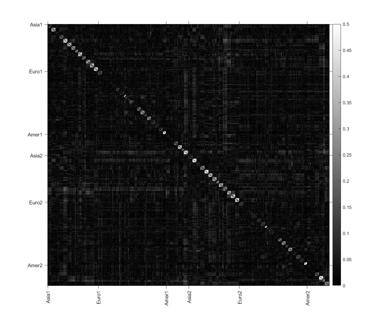
Figure 8: The absolute values of the elements of $S_{yy}-\hat{\Sigma}_{yy}^{*}$. “Asia1” denotes the first Asia-Pacific index in “day one”, while “Asia2” denotes the first Asia-Pacific index in “day two”, and so forth.

Figure 9 displays the rows of $S_{yy}$ or $\hat{\Sigma}_{yy}^{*}$ corresponding to the Large-Value indices of Mainland China, Japan, Hong Kong, UK, and US in “day one”. The red and blue lines in a sub-plot represent the corresponding row of $S_{yy}$ and $\hat{\Sigma}_{yy}^{*}$, respectively. The closeness of the two lines indicates that our model fits the data rather well for these main markets.

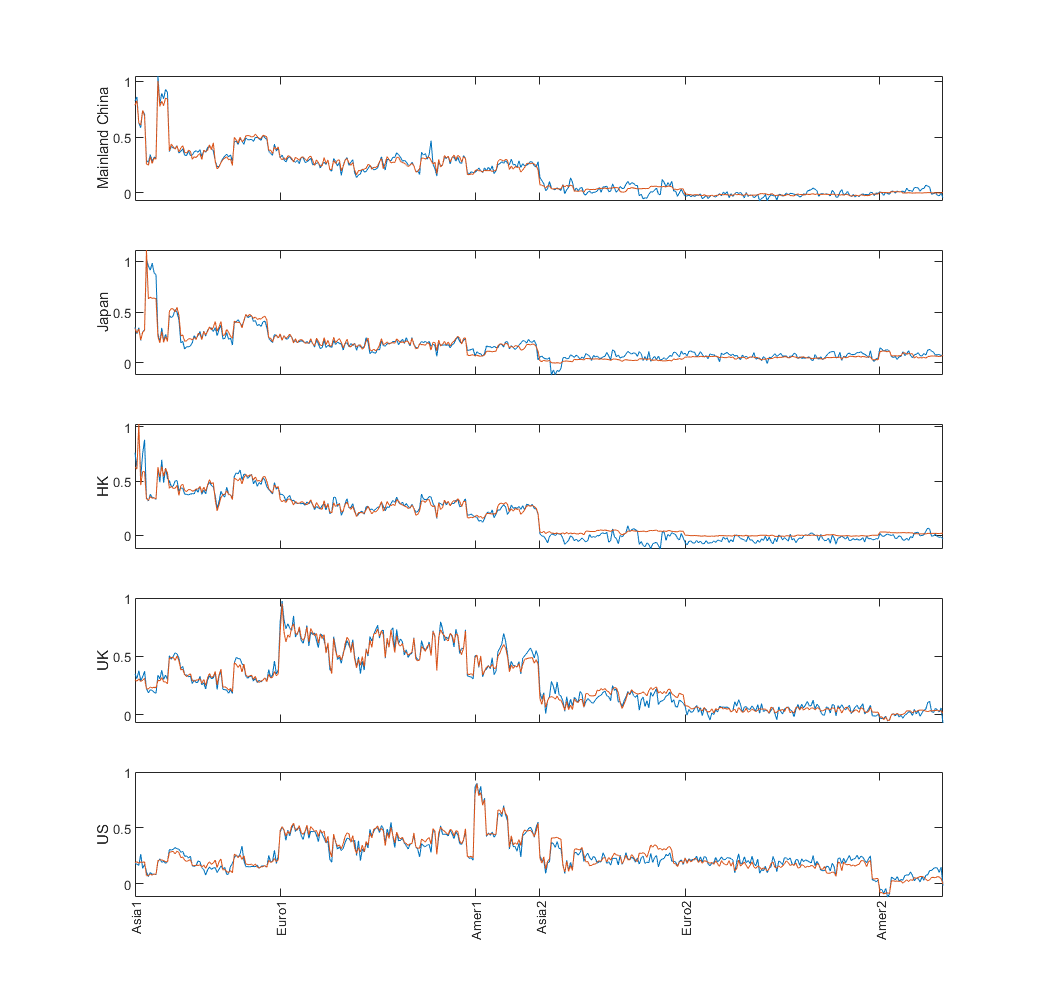
Figure 9: The rows of $S_{yy}$ or $\hat{\Sigma}_{yy}^{*}$ corresponding to the Large-Value indices of Mainland China, Japan, Hong Kong, UK, and US in “day one”. The red and blue lines in a sub-plot represent the corresponding row of $S_{yy}$ and $\hat{\Sigma}_{yy}^{*}$, respectively.

We further calculate the average absolute value, denoted $d_{o}$, of the elements of $S_{yy}-\hat{\Sigma}_{yy}^{*}$ for pairs of indices that have overlapping sub-periods (e.g., the Japanese Large-Growth index in “day one” and the US Mid-Value index in “day two”), excluding pairs that are in the same market. We repeat the calculation, denoted $d_{n}$, for pairs of indices that have no overlapping sub-periods, excluding pairs that are in the same market. If the global stock markets are fully efficient, the sample covariance of a non-overlapping-sub-periods pair, given by the corresponding element of $S_{yy}$, should be close to 0. The corresponding fitted element of $\hat{\Sigma}_{yy}^{*}$ should also be close to 0 given our model structure. In this case, the non-zero value of the element of $S_{yy}-\hat{\Sigma}_{yy}^{*}$ corresponds to a non-overlapping-sub-periods pair is probably due to noise, not some factor missing from our model. Thus $d_{n}$ could serve as the benchmark for noise. In our sample, both $d_{n}$ and $d_{o}$ are around 0.0304, which suggests that our model also fits the overlapping-sub-periods pairs reasonably well.

6.4 Market Connectivity under Different VIX Levels

In this section, we investigate whether market connectivity increases when the US VIX increases. Specifically, we divide the sample into two sub-samples according to the level of the VIX. Since our QML estimators ignore the cross-$t$-period correlation, we could assign non-consecutive time units to a sub-sample, something we cannot do when using the MLE. Nevertheless, in order to maintain some extent of temporal continuity, we assign time units from months that exceed the median monthly VIX into the high-VIX sub-sample, while that below the median monthly VIX into the low-VIX sub-sample.

We conduct this analysis for two separate time intervals: one from May 5th, 2014 to Nov 29th, 2018 (the before sub-sample), and the other from Nov 30th, 2018 to June 23rd, 2023 (the after sub-sample). Consequently, we have a total of four sub-samples: Before-HighVix, Before-LowVix, After-HighVix, and After-LowVix, where Before-HighVix is the intersection of the before and high-VIX sub-samples, and so forth. Figure 10 illustrates these sub-samples. The grey shaded regions depict the HighVix sub-sample; the red dashed line indicates Nov 29th, 2018.

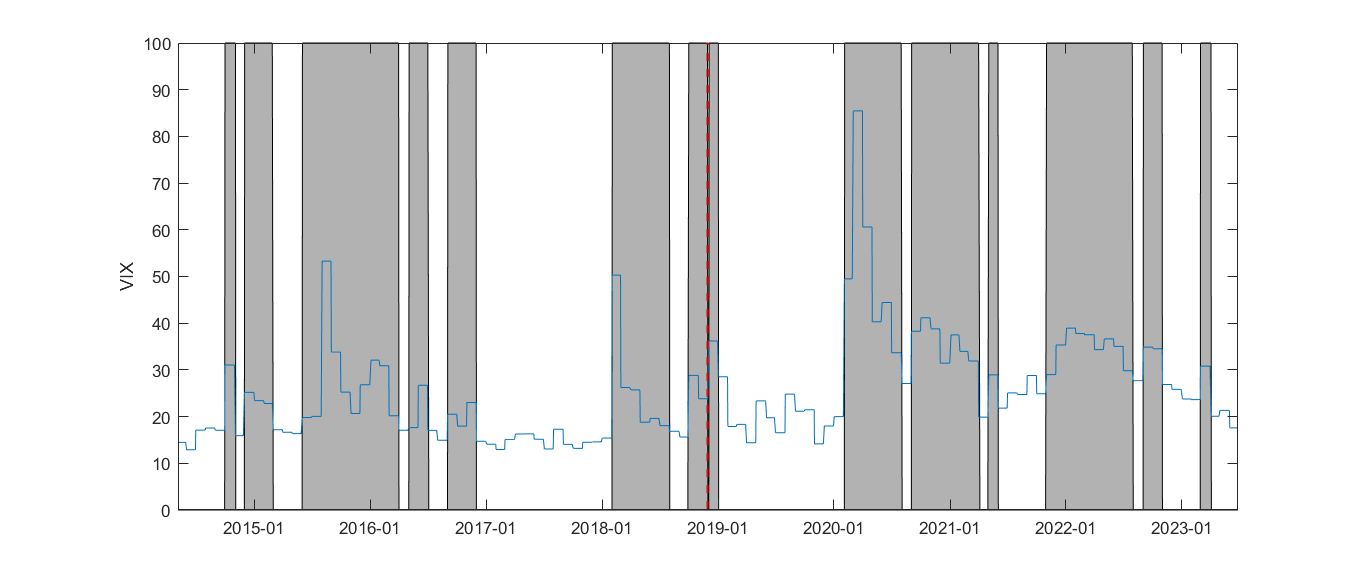
Figure 10: The grey shaded regions depict the HighVix sub-sample; the red dashed line indicates Nov 29th, 2018. The light blue line indicates the VIX.

The HighVix sub-sample consists of the time units mainly after Nov 29th, 2018, while the LowVix sub-sample consists of the time units mainly before Nov 29th, 2018. Thus, it is possible that the HighVix and LowVix sub-samples differ in aspects other than the VIX. For example, the Covid-19 happened in the after sub-sample. We argue that the Before-HighVix and Before-LowVix sub-samples are more alike in aspects other the VIX, similarly for the After-HighVix and After-LowVix sub-samples. That is the reason we partition the sample into the four sub-samples.

We estimate the model for each of the four sub-samples. Table 11 presents the average value of the non-integration or global integration indices of all the markets within each continent for each sub-sample. The average value of the non-integration indices is bigger in the Before-LowVix sub-sample than in the Before-HighVix sub-sample for each continent; the pattern also holds for the After-LowVix and After-HighVix sub-samples. Moreover, the average value of global integration indices is bigger in the Before-HighVix sub-sample than in the Before-LowVix sub-sample for each continent, similarly for the After-HighVix and After-LowVix sub-samples. This implies that the markets become more integrated during periods of high VIX.

Non-integration	Before-LowVix	Before-HighVix	After-LowVix	After-HighVix
Asia-Pacific	0.6274	0.3554	0.4721	0.3790
Europe	0.4782	0.2646	0.4055	0.2932
Americas	0.4000	0.2802	0.4163	0.2209
Global integration	Before-LowVix	Before-HighVix	After-LowVix	After-HighVix
Asia-Pacific	0.2642	0.5761	0.4944	0.5286
Europe	0.3024	0.5753	0.3286	0.4303
Americas	0.5001	0.6324	0.4495	0.6873

Table 11: The average value of the non-integration or global integration indices of all the markets within each continent for each sub-sample.

	Before-LowVix	Before-HighVix	After-LowVix	After-HighVix
Ave. of $|\boldsymbol{\beta}_{\text{asia,a\_time}}^{G}|$	0.2818	0.4989	0.5473	0.6840
Ave. of $|\boldsymbol{\beta}_{\text{euro,a\_time}}^{G}|$	0.3354	0.6128	0.4867	0.5139
Ave. of $|\boldsymbol{\beta}_{\text{amer,a\_time}}^{G}|$	0.3500	0.6027	0.4638	0.7195
Ave. of $|\boldsymbol{\beta}_{\text{asia,e\_time}}^{G}|$	0.2041	0.2044	0.3489	0.2057
Ave. of $|\boldsymbol{\beta}_{\text{euro,e\_time}}^{G}|$	0.2475	0.3977	0.1776	0.2050
Ave. of $|\boldsymbol{\beta}_{\text{amer,e\_time}}^{G}|$	0.4191	0.1791	0.1208	0.2581
Ave. of $|\boldsymbol{\beta}_{\text{asia,am\_time}}^{G}|$	0.2030	0.4534	0.2686	0.1130
Ave. of $|\boldsymbol{\beta}_{\text{euro,am\_time}}^{G}|$	0.0700	0.0541	0.0894	0.1411
Ave. of $|\boldsymbol{\beta}_{\text{amer,am\_time}}^{G}|$	0.1417	0.4368	0.4212	0.5072
Ave. of $|\boldsymbol{\beta}_{\text{asia}}|$	0.2384	0.2186	0.1686	0.2436
Ave. of $|\boldsymbol{\beta}_{\text{euro}}|$	0.4414	0.4458	0.5132	0.5223
Ave. of $|\boldsymbol{\beta}_{\text{amer}}|$	0.2218	0.2289	0.2288	0.2984

Table 12: The average absolute value of loadings of a continent for a sub-period of a day for a sub-sample.

Table 12 displays the average absolute value of loadings of a continent for a sub-period of a day for a sub-sample. For all three continents, the global factor has larger average absolute values of the loadings during the Asian sub-period in the high VIX sub-samples than in the low VIX sub-samples. This means that the international news happened during the Asian sub-period becomes more influential when the VIX increases. On the other hand, the loadings of the continental factors remain roughly the same in terms of either the average absolute values reported in Table 12 or the individual absolute values (available upon request).

In summary, our findings indicate that the global integration increases when the VIX increases. This is primarily driven by the increase of the magnitudes of loadings of the global factor during the Asian sub-period. We also conduct the misspecification checks of Section 6.3 using the four sub-samples in Section LABEL:sec_add_application of the OS.

7 Conclusion

In this paper, we introduce a confirmatory dynamic factor model to model a large number of daily stock returns across different time zones. This model accounts for the impacts of both the global and continental factors, and provides means to assess the efficient market hypothesis and levels of international and regional integration. We extend Bai and Li (2012)’s results to this large confirmatory dynamic factor model. This has practical importance because economic or financial theories often imply confirmatory factor models whose identification schemes do not comply with those of Bai and Li (2012). We apply our model to the 42 markets and find that the US is the most integrated market, and the global market exhibits higher integration when the VIX is large.

References

- Acharya et al. (2012) Acharya, V., R. Engle, and M. Richardson (2012). Capital shortfall: A new approach to ranking and regulating systemic risks. American Economic Review: Papers and Proceedings 102(3), 59–64.
- Aruoba et al. (2009) Aruoba, S. B., F. X. Diebold, and C. Scotti (2009). Real-time measurement of business conditions. Journal of Business & Economic Statistics 27(4), 417–427.
- Bai and Li (2012) Bai, J. and K. Li (2012). Statistical analysis of factor models of high dimension. The Annals of Statistics 40(1), 436–465.
- Bai and Li (2016) Bai, J. and K. Li (2016). Maximum likelihood estimation and inference for approximate factor models of high dimension. The Review of Economics and Statistics 98(2), 298–309.
- Banbura et al. (2013) Banbura, M., D. Giannone, M. Modugno, and L. Reichlin (2013). Nowcasting and the real-time data flow. In G. Elliott and A. Timmermann (Eds.), Handbook of Economic Forecasting, Volume 2, Chapter 4, pp. 195–237. Elsevier, North-Holland.
- Banbura et al. (2011) Banbura, M., D. Giannone, and L. Reichlin (2011). Nowcasting. The Oxford Handbook of Economic Forecasting.
- Barigozzi (2023) Barigozzi, M. (2023). Quasi maximum likelihood estimation of high-dimensional factor models: A critical review. arXiv preprint arXiv: 2303.11777.
- Barigozzi et al. (2019) Barigozzi, M., M. Hallin, and S. Soccorsi (2019). Identification of global and local shocks in international financial markets via general dynamic factor models. Journal of Financial Econometrics 17, 462–494.
- Barigozzi and Luciani (2022) Barigozzi, M. and M. Luciani (2022). Quasi maximum likelihood estimation and inference of large approximate dynamic factor models via the EM algorithm. arXiv preprint arXiv:1910.03821v3.
- Bekaert et al. (2014) Bekaert, G., M. Ehrmann, M. Fratzscher, and A. Mehl (2014). The global crisis and equity market contagion. The Journal of Finance 69(6), 2597–2649.
- Bekaert et al. (2009) Bekaert, G., R. J. Hodrick, and X. Zhang (2009). International stock return comovements. The Journal of Finance 64(6), 2591–2626.
- Bekaert et al. (2023) Bekaert, G., M. Hoerova, and N. R. Xu (2023). Risk, monetary policy and asset prices in a global world. Available at SSRN 3599583.
- Bekaert and Mehl (2019) Bekaert, G. and A. Mehl (2019). On the global financial market integration “swoosh” and the trilemma. Journal of International Money and Finance 94, 227–245.
- BenSaïda (2019) BenSaïda, A. (2019). Good and bad volatility spillovers: An asymmetric connectedness. Journal of Financial Markets 43, 78–95.
- Burns et al. (1998) Burns, P., R. Engle, and J. Mezrich (1998). Correlations and volatilities of asynchronous data. Journal of Derivatives 5(4), 7.
- Cai et al. (2009) Cai, Y., R. Y. Chou, and D. Li (2009). Explaining international stock correlations with CPI fluctuations and market volatility. Journal of Banking & Finance 33(11), 2026–2035. Financial Globalisation, Risk Analysis and Risk Management.
- Cappiello et al. (2006) Cappiello, L., R. F. Engle, and K. Sheppard (2006). Asymmetric dynamics in the correlations of global equity and bond returns. Journal of Financial econometrics 4(4), 537–572.
- Corsetti et al. (2005) Corsetti, G., M. Pericoli, and M. Sbracia (2005). ‘some contagion, some interdependence’: More pitfalls in tests of financial contagion. Journal of International Money and Finance 24(8), 1177–1199.
- Doz et al. (2012) Doz, C., D. Giannone, and L. Reichlin (2012). A quasi-maximum likelihood approach for large, approximate dynamic factor models. The Review of Economics and Statistics 94(4), 1014–1024.
- Dungey and Gajurel (2015) Dungey, M. and D. Gajurel (2015). Contagion and banking crisis-international evidence for 2007-2009. Journal of Banking & Finance 60, 271–283.
- Engle et al. (2015) Engle, R., E. Jondeau, and M. Rockinger (2015). Systemic risk in Europe. Review of Finance 19(1), 145–190.
- Engle (2016) Engle, R. F. (2016). Dynamic conditional beta. Journal of Financial Econometrics 14(4), 643–667.
- Forbes and Rigobon (2002) Forbes, K. J. and R. Rigobon (2002). No contagion, only interdependence: Measuring stock market comovements. The Journal of Finance 57(5), 2223–2261.
- Forni et al. (2000) Forni, M., M. Hallin, M. Lippi, and L. Reichlin (2000). The generalized dynamic-factor model: Identification and estimation. The Review of Economics and Statistics 82(4), 540–554.
- Gagnon and Karolyi (2006) Gagnon, L. and G. A. Karolyi (2006). Price and volatility transmission across borders. Financial Markets, Institutions & Instruments 15(3), 107–158.
- Gagnon and Karolyi (2009) Gagnon, L. and G. A. Karolyi (2009). Information, trading volume, and international stock return comovements: Evidence from cross-listed stocks. Journal of Financial and Quantitative Analysis 44(4), 953–986.
- Giannone et al. (2008) Giannone, D., L. Reichlin, and D. Small (2008). Nowcasting: the real-time informational content of macroeconomic data. Journal of Monetary Economics 55, 665–676.
- Hallin and Liška (2011) Hallin, M. and R. Liška (2011). Dynamic factors in the presence of blocks. Journal of Econometrics 163, 29–41.
- He and Hamori (2021) He, X. and S. Hamori (2021). Is volatility spillover enough for investor decisions? a new viewpoint from higher moments. Journal of International Money and Finance 116, 102412.
- Jöreskog (1969) Jöreskog, K. G. (1969). A general approach to confirmatory maximum likelihood factor analysis. Psychometrika 34, 183–202.
- Koch and Koch (1991) Koch, P. D. and T. W. Koch (1991). Evolution in dynamic linkages across daily national stock indexes. Journal of International Money and Finance 10, 231–251.
- Kose et al. (2003) Kose, M. A., C. Otrok, and C. H. Whiteman (2003). International business cycles: World, region and country-specific factors. The American Economic Review 93(4), 1216–1239.
- Lehkonen (2015) Lehkonen, H. (2015). Stock market integration and the global financial crisis. Review of Finance 19(5), 2039–2094.
- Lin et al. (1994) Lin, W.-L., R. F. Engle, and T. Ito (1994). Do bulls and bears move across borders? international transmission of stock returns and volatility. The Review of Financial Studies 7(3), 507–538.
- Marshall et al. (2021) Marshall, B. R., H. T. Nguyen, N. H. Nguyen, and N. Visaltanachoti (2021). Country governance and international equity returns. Journal of Banking & Finance 122, 105986.
- Niţoi and Pochea (2019) Niţoi, M. and M. M. Pochea (2019). What drives european union stock market co-movements? Journal of International Money and Finance 97, 57–69.
- Opie and Riddiough (2020) Opie, W. and S. J. Riddiough (2020). Global currency hedging with common risk factors. Journal of Financial Economics 136(3), 780–805.
- Pan and Connett (2002) Pan, W. and J. E. Connett (2002). Selecting the working correlation structure in generalized estimation equations with application to the lung health study. Statistica Sinica 12, 475–490.
- Pukthuanthong and Roll (2009) Pukthuanthong, K. and R. Roll (2009). Global market integration: An alternative measure and its application. Journal of Financial Economics 94(2), 214–232.
- Quah and Sargent (1993) Quah, D. and T. J. Sargent (1993). A dynamic index model for large cross sections. In J. H. Stock and M. W. Watson (Eds.), Business Cycles, Indicators and Forecasting, pp. 285 – 310. University of Chicago Press.
- Rapach et al. (2013) Rapach, D. E., J. K. Strauss, and G. Zhou (2013). International stock return predictability: What is the role of the United States? The Journal of Finance 68(4), 1633–1662.
- Rubin and Thayer (1982) Rubin, D. B. and D. T. Thayer (1982). EM algorithms for ML factor analysis. Psychometrika 47(1), 69–76.
- Savva et al. (2009) Savva, C. S., D. R. Osborn, and L. Gill (2009). Spillovers and correlations between US and major European stock markets: the role of the euro. Applied Financial Economics 19(19), 1595–1604.
- Schotman and Zalewska (2006) Schotman, P. C. and A. Zalewska (2006). Non-synchronous trading and testing for market integration in central european emerging markets. Journal of Empirical Finance 13(4), 462–494. Special Issue: International Finance.
- Sharma and Seth (2012) Sharma, A. and N. Seth (2012). Literature review of stock market integration: a global perspective. Qualitative Research in Financial Markets 4(1), 84–122.
- Stock and Watson (2016) Stock, J. H. and M. W. Watson (2016). Dynamic factor models, factor-augmented vector autoregressions, and structural vector autoregressions in macroeconomics. In Handbook of Macroeconomics, Volume 2, Chapter 8, pp. 415–525. Elsevier B.V.
- van der Vaart (1998) van der Vaart, A. (1998). Asymptotic Statistics. Cambridge University Press.
- Watson and Engle (1983) Watson, M. W. and R. F. Engle (1983). Alternative algorithms for the estimation of dynamic factor, mimic and varying coefficient regression models. Journal of Econometrics 23, 385–400.