Invertible Tabular GANs: Killing Two Birds with One Stone for Tabular Data Synthesis
Abstract
Tabular data synthesis has received wide attention in the literature. This is because available data is often limited, incomplete, or cannot be obtained easily, and data privacy is becoming increasingly important. In this work, we present a generalized GAN framework for tabular synthesis, which combines the adversarial training of GANs and the negative log-density regularization of invertible neural networks. The proposed framework can be used for two distinctive objectives. First, we can further improve the synthesis quality, by decreasing the negative log-density of real records in the process of adversarial training. On the other hand, by increasing the negative log-density of real records, realistic fake records can be synthesized in a way that they are not too much close to real records and reduce the chance of potential information leakage. We conduct experiments with real-world datasets for classification, regression, and privacy attacks. In general, the proposed method demonstrates the best synthesis quality (in terms of task-oriented evaluation metrics, e.g., F1) when decreasing the negative log-density during the adversarial training. If increasing the negative log-density, our experimental results show that the distance between real and fake records increases, enhancing robustness against privacy attacks.
1 Introduction
Generative models, such as generative adversarial networks (GANs) and variational autoencoders (VAEs), have proliferated over the past several years [24, 15, 31, 2, 18, 1, 16]. GANs are one of the most successful models among generative models, and tabular data synthesis is one of the many GAN applications [7, 4, 28, 27, 21, 38].
However, tabular data synthesis is challenging due to the following two problems: i) Tabular data frequently contains sensitive information. ii) It is required to share tabular data with people, some of whom are trustworthy while others are not. Therefore, generating fake records as similar as possible to real ones, which is commonly accepted to enhance the synthesis quality, is not always preferred in tabular data synthesis, e.g., sharing with unverified people [27, 5].
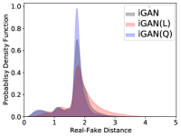
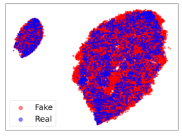
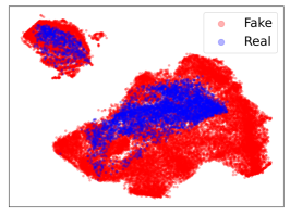
In [5], it was revealed that one can effectively extract privacy-related information from a pre-trained GAN model if its log-densities are high enough. To this end, we propose a generalized framework, called invertible tabular GAN (IT-GAN), where we integrate the adversarial training of GANs and the negative log-density training of invertible neural networks. In our framework, we can improve111It is well known that VAEs generate blurred samples but achieve a better log-density than GANs. Therefore, there exists a room to improve the log-density of fake samples by GANs. or sacrifice the negative log-density during the adversarial training to trade off between synthesis quality and privacy protection (cf. Figure 1).
Our generator based on neural ordinary differential equations (NODEs [6]) is invertible and enables the proposed training concept. For NODEs, there exists an efficient unbiased estimation technique of their Jacobian-determinants [6, 16]. By using the unbiased Hutchinson estimator, therefore, we can efficiently estimate the negative log-density. After that, this negative log-density can be used for the following two opposite objectives: i) decreasing the negative log-density to further increase the synthesis quality (cf. IT-GAN(Q) in Figure 1), or ii) increasing the negative log-density to synthesize realistic fake records that are not too much similar to real records (cf. IT-GAN(L) in Figure 1). In particular, the second objective to make the log-density worse after little sacrificing the synthesis quality is closely related to the information leakage issue of tabular data.
However, this invertible generator has one limitation – the dimensionality of hidden layers cannot be changed. To overcome this limitation, we propose a joint architecture of an autoencoder (AE) and a GAN. The motivation behind the proposed joint architecture is twofold: i) The role of the AE is to create a hidden representation space, on which the generator and the discriminator work. The hidden representation space has the same dimensionality as that of the latent input vector of the generator. Therefore, the input and output sizes are the same in our generator, which meets the invariant dimensionality requirement of NODEs. ii) Separating the labor between the AE and the generator can improve the training process. In general, tabular data contains a large number of columns, which makes the synthesis more difficult. In our joint architecture, the generator shares its task with the AE; it does not directly synthesize fake records but fake hidden representations. The decoder (recovery network) of the AE converts them into human-readable fake records. Therefore, our final training consists of the GAN training, the AE training, and the negative log-density regularization.
We conduct experiments with 6 real-world tabular datasets and compare our method with 9 baseline methods. In many evaluation cases, our methods outperform all other baselines. Our contributions can be summarized as below:
-
1.
We propose a general framework where we can trade-off between synthesis quality and information leakage.
-
2.
To this end, we combine the adversarial training of GANs and the negative log-density training of invertible neural networks.
-
3.
We conduct thorough experiments with 6 real-world tabular datasets and our methods outperform existing methods in almost all cases.
2 Related Work
We introduce various tabular data synthesis methods and invertible neural networks. In particular, we review the invertible characteristic of NODEs.
2.1 Table Data Synthesis
Let be a tabular data which consists of columns. Each column of is either discrete or continuous numerical. Let be a record of . The goal of tabular data synthesis is i) to learn a density that best approximates the data distribution and ii) to generate a fake tabular data . For simplicity without loss of generality, we assume , i.e., the real and fake tabular data have the same number of records.
This take can be accomplished by various approaches, e.g., VAEs, GANs, and so forth, to name a few. We introduce a couple of seminal models in this field. Tabular data synthesis, which generates a realistic synthetic table by modeling a joint probability distribution of columns in a table, encompasses many different methods depending on the types of data. For instance, Bayesian networks [3, 42] and decision trees [30] are used to generate discrete variables. A recursive modeling of tables using the Gaussian copula is used to generate continuous variables [29]. A differentially private algorithm for decomposition is used to synthesize spatial data [9, 41]. However, some constraints that these models have such as the type of distributions and computational problems have hampered high-fidelity data synthesis.
In recent years, several data generation methods based on GANs have been introduced to synthesize tabular data, which mostly handle continuous/discrete numerical records. RGAN [13] generates continuous time-series healthcare records while MedGAN [7], CorrGAN [28] generate discrete discrete records. EhrGAN [4] generates plausible labeled records using semi-supervised learning to augment limited training data. PATE-GAN [21] generates synthetic data without endangering the privacy of original data. TableGAN [27] improved tabular data synthesis using convolutional neural networks to maximize the prediction accuracy on the label column. TGAN [38] is one of the most recent conditional GAN-based models. It suggested a couple of important directions toward high-fidelity tabular data synthesis, e.g., a preprocessing mechanism to convert each record into a form suitable for GANs.
2.2 Invertible Neural Networks and Neural Ordinary Differential Equations
Invertible neural networks are typically bijective. Owing to this property and the change of variable theorem, we can efficiently calculate the exact log-density of data sample as follows:
| (1) |
where is an invertible function, and . is the Jacobian of , which is the most computationally demanding part to calculate — it has a cubic time complexity. Therefore, invertible neural networks typically restrict the Jacobian matrix definition into a form that can be efficiently calculated [31, 36, 25, 26, 10, 11]. However, FFJORD [16] recently proposed a NODE-based invertible architecture where we can use any form of Jacobian and we also rely on this technique.
In NODEs [6], let be a hidden vector at time (or layer) in a neural network. NODEs solve the following integral problem to calculate from [6]:
| (2) |
where , which we call ODE function, is a neural network to approximate . To solve the integral problem, NODEs rely on ODE solvers, e.g., the explicit Euler method, the Dormand–Prince method, and so forth [12]. is easily reconstructed from with a reverse-time ODE as follows:
| (3) |
Two other related papers are FlowGAN [17] and TimeGAN [39] although they do not synthesize tabular data. FlowGAN combines the adversarial training with NICE [10] or RealNVP [11]. Grover et al. showed in the paper that likelihood-based training does not show reliable synthesis for high-dimensional space and they attempt to combine them [17]. TimeGAN also combines, given time-series data, the adversarial training and the supervised likelihood training of predicting a next value from past values. This supervised training is available because they deal with time-series data. In our case, we combine the adversarial training and the negative log-density regularization of NODEs, which are considered as more general than NICE and RealNVP [16].
3 Proposed Method
We propose a more advanced setting for tabular data synthesis than those of existing methods. Our goal is to integrate the adversarial training of GANs and the log-density training of invertible neural networks. Therefore, one can easily trade off between synthesis quality and privacy protection.
We describe our design in this section. The two key points in our design are that i) we use an invertible neural network architecture to design our generator, and ii) we integrate an AE into our framework to ii-a) enable the isometric architecture of the generator, i.e., the dimensions of hidden layers do not vary, and ii-b) distribute the workload of the generator.
3.1 Overall Architecture
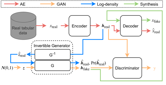
The overall architecture is in Figure 2. Our architecture can be classified into the following four data paths: AE-path) The AE data path, highlighted in red, is related to an AE model to generate, given a real record , a hidden representation and reconstruct . Log-density-path) There are two different data paths related to the generator. The log-density path, highlighted in blue, is related to an invertible model to calculate the log-density of the hidden representation , i.e., . Therefore, we can consider it as the log-density of the real record because the hidden representation is from the real record. GAN-path) The second data path related to the generator, highlighted in orange, is for the adversarial training. The discriminator reads and , which is generated by the generator from the latent vector , to distinguish them. Synthesis-path) The last data path, highlighted in green, is used after finishing training our model. Using the generator and the decoder, we synthesize many fake records.
3.2 Autoencoder
We describe our AE model in this subsection. Our AE model relies on the mode-specific normalization, which i) fits a variational mixture of Gaussians for each continuous column of , ii) converts each continuous element of -th record into a one-hot vector denoting the specific Gaussian that best matches the element and its scalar normalized value in the selected Gaussian. If a column is discrete, we simply convert each value in the column into a one-hot vector. After that we use the following encoder and the decoder (recovery network) :
| (4) | ||||
| (5) |
where is a ReLU, is fully connected layer which takes the size of input. Through several fully connected layers, makes the size of output. We use to denote the parameters of the encoder. Analogously, takes the size of input, and after several FC layers makes the size of output. We use to denote the parameters of the decoder (recovery network).
3.3 Generator
The key point in our generator design is to adopt an invertible neural network [16] for our own purposes. Among various invertible architectures, we adopt and customize NODEs. The NODE-based invertible models have the advantage that there are no restrictions on the form of Jacobian-determinant. Other invertible models typically restrict their Jacobian-determinants to specific forms that can be easily calculated. However, our NODE-based model does not have such restrictions.
Therefore, we could study about the generator architecture without any restrictions and finally use the following architecture for our generator :
| (6) | ||||
where is a non-linear activation, and are with (, ), and are with (, ), and and are with (, ) if . is a latent vector sampled from the unit Gaussian. is the mapping function which defines a proportion between and . We use either or for , where means concatenation. In our case, . In fact, this invariant dimensionality is one characteristic of many invertible neural networks. We use to denote the parameters of the generator.
The integral problem can be solved by various ODE solvers. The log-probability can be calculated, by the unbiased Hutchinson estimator, as follows:
| (7) |
where is a standard Gaussian or Rademacher distribution [19]. The time complexity to calculate the Hutchinson estimator is slightly larger than that of evaluating since the vector-Jacobian product has the same cost as that of evaluating using the reverse-mode automatic differentiation.
One distinguished property of the generator is, given a real hidden vector , that we can reconstruct by and estimate its log-probability , where by exactly solving Eq. (3) — note that is analytically defined from G and requires no training.
3.4 Discriminator
The discriminator reads and to classify them. We use the following architecture:
| (8) |
where takes the size of input, and after several FC layers makes the one dimension output. is a Leaky ReLU with negative slope, and is a dropout with a ratio of . We use to denote the parameters of the discriminator.
3.5 Training Algorithm
We describe how to train the proposed architecture. Since it consists of several modules and their loss functions, we first separately describe them and then, the final training algorithm.
Loss Functions.
We introduce various loss functions we use to train our model. First, we use the following AE loss to train the encoder and the decoder model:
| (9) |
where is a typical reconstruction error loss. We note that we here want to learn a sparse encoder with the regularization term. is a hidden vector generated by the generator G. is a reconstructed hidden vector by , where E and R mean the encoder and the decoder, respectively. After some preliminary studies, we found that this loss definition provides robust training in many cases. In particular, it further stabilizes the integrity of the autoencoder in terms of the learned hidden representation space. To train the generator and the discriminator, we use the WGAN-GP loss. Then, we propose to use the following regularizer to control the log-density, which results in an adjustment of the real-fake distance:
| (10) |
where E is the encoder, is a coefficient to emphasize the regularization, and the log-density can be calculated with Eq. (7) during .
Training Algorithm.
Algorithm 1 describes our training method. There is a training data . We first train the encoder with the AE and WGAN-GP losses and the decoder with the AE loss (line 1). To learn a hidden vector space that is suitable for the overall synthesis process, we train the encoder with the WGAN-GP loss to help the discriminator better distinguish real and fake hidden vectors by learning a hidden vector in favor of the discriminator. By doing this, the AE and the GAN are integrated into a single framework. Then we train the discriminator with the WGAN-GP loss every (line 1), the generator with the WGAN-GP loss every (line 1). After that, the generator is trained one more time with the proposed density regularizer every (line 1). Since the discriminator and the generator rely on the hidden vector created by the AE model, we then train the encoder and the decoder every iteration. The log-density regularization is also not always used but every iteration because we found that a frequent log-density regularization negatively affects the entire training progress. Using the validation data and a task-oriented evaluation metric, we choose the best model. For instance, we use the F-1/MSE score of a trained generator every epoch with the validating data — an epoch consists of many iterations depending on the number of records in the training data and a mini-batch size. If a recent model is better than the temporary best model, we update it.
On the Tractability of Training the Generator.
The ODE version of the Cauchy–Kowalevski theorem states that, given , there exists a unique solution of if is analytic (or locally Lipschitz continuous). In other words, the ODE problem is well-posed if is analytic [14]. In our case, the function in Eq. (6) uses various FC layers that are analytic and some non-linear activations that may or may not be analytic. However, the hyperbolic tangent (tanh), which is analytic, is mainly used in our experiments. This implies that there will be only one unique optimal ODE for the generator, given a latent vector . Because of i) the uniqueness of the solution and ii) our relatively simpler definitions of in comparison with other NODE applications, e.g., convolutional layer followed by a ReLU in [6], we believe that our training method can find a good solution for the generator.
4 Experimental Evaluations
We introduce our experimental environments and results for tabular data synthesis. Experiments were done in the following software and hardware environments: Ubuntu 18.04, Python 3.7.7, Numpy 1.19.1, Scipy 1.5.2, PyTorch 1.8.1, CUDA 11.2, and NVIDIA Driver 417.22, i9 CPU, and NVIDIA RTX Titan.
| Method | F1 | ROCAUC | |
| Real | 0.66±0.00 | 0.88±0.00 | |
| PrivBN | 0.43±0.02 | 0.84±0.01 | |
| TVAE | 0.62±0.01 | 0.84±0.01 | |
| TGAN | 0.63±0.01 | 0.85±0.01 | |
| TableGAN | 0.46±0.03 | 0.81±0.01 | |
| IT-GAN(Q) | 0.64±0.01 | 0.86±0.00 | |
| IT-GAN(L) | 0.64±0.01 | 0.85±0.01 | |
| IT-GAN | 0.64±0.01 | 0.86±0.01 |
| Method | F1 | ROCAUC |
| Real | 0.47±0.01 | 0.90± 0.00 |
| PrivBN | 0.23±0.03 | 0.81±0.03 |
| TVAE | 0.44±0.01 | 0.86±0.01 |
| TGAN | 0.38±0.03 | 0.86±0.02 |
| TableGAN | 0.31±0.06 | 0.81±0.03 |
| IT-GAN(Q) | 0.45±0.01 | 0.89±0.00 |
| IT-GAN(L) | 0.46±0.01 | 0.88±0.01 |
| IT-GAN | 0.45±0.01 | 0.88±0.00 |
| Method | Macro F1 | Micro F1 | ROCAUC |
| Real | 0.48±0.01 | 0.61±0.00 | 0.67±0.00 |
| Ind | 0.27±0.01 | 0.44±0.01 | 0.51±0.01 |
| PrivBN | 0.32±0.02 | 0.51±0.01 | 0.60±0.00 |
| TVAE | 0.39±0.00 | 0.57±0.00 | 0.58±0.00 |
| TGAN | 0.40±0.00 | 0.55±0.01 | 0.59±0.00 |
| MedGAN | 0.37±0.02 | 0.51±0.03 | 0.56±0.01 |
| IT-GAN(Q) | 0.41±0.01 | 0.54±0.01 | 0.60±0.00 |
| IT-GAN(L) | 0.40±0.01 | 0.55±0.01 | 0.60±0.01 |
| IT-GAN | 0.40±0.00 | 0.54±0.01 | 0.59±0.01 |
| Method | Macro F1 | Micro F1 | ROCAUC |
| Real | 0.65±0.00 | 0.68±0.00 | 0.78±0.00 |
| PrivBN | 0.64±0.00 | 0.67±0.00 | 0.77±0.00 |
| TVAE | 0.60±0.02 | 0.66±0.01 | 0.74±0.01 |
| TGAN | 0.64±0.00 | 0.67±0.00 | 0.76±0.00 |
| VeeGAN | 0.54±0.06 | 0.60±0.05 | 0.71±0.02 |
| IT-GAN(Q) | 0.66±0.00 | 0.69±0.00 | 0.79±0.01 |
| IT-GAN(L) | 0.66±0.01 | 0.68±0.01 | 0.79±0.00 |
| IT-GAN | 0.64±0.01 | 0.67±0.01 | 0.77±0.00 |
4.1 Experimental Environments
4.1.1 Datasets
We test with various real-world tabular data, targeting binary/multi-class classification and regression. Their statistics are summarized in Appendix A. The list of datasets is as follows: Adult [32] consists of diverse demographic information in the U.S., extracted from the 1994 Census Survey, where we predict two classes of high ($50K) and low ($50K) income. Census [33] is similar to Adult but it has different columns. Credit [40] is for bank loan status prediction. Cabs [34] is collected by an Indian cab aggregator service company for predicting the types of customers. King [23] contains house sale prices for King County in Seattle for the records between May 2014 and May 2015. News [22] has a heterogeneous set of features about articles published by Mashable in a period of two years, to predict the number of shares in social networks. Adult and Census are for binary classification, and Credit and Cabs are for multi-class classification. The others are for regression.
4.1.2 Evaluation Methods
We generate fake tabular data and train multiple classification (SVM, DecisionTree, AdaBoost, and MLP) or regression (Linear Regression and MLP) algorithms. We then evaluate them with testing data and average their performance in terms of various evaluation metrics. This specific evaluation method was proposed in [38] and we follow their evaluation protocol strictly. We execute these procedures five times with five different seed numbers.
For our IT-GAN, we consider IT-GAN(Q) with a positive , which decreases the negative log-density to improve the synthesis Quality, IT-GAN(L), which sacrifices the log-density to decrease the information Leakage with a negative , and IT-GAN, which does not use the log-density regularization. In our result tables, Real means that we use real tabular data to train a classification/regression model. For other baselines, refer to Appendix C.
We do not report some baselines in our result tables to save spaces if their results are significantly worse than others. We refer to Appendix E for their full result tables.
4.1.3 Hyperparameters
We consider the following ranges of the hyperparameters: the numbers of layers in the encoder and the decoder, and , are in {2, 3}. The number of layers of Eq. (8) is in {2, 3}. Dropout ratio is in {0, 0.5}, and the leaky relu slope is in {0, 0.2}. The non-linear activation is tanh; the multiplication factor of Eq. (6) is in {1, 1.5}; the number of layers of Eq. (6) is in {3}; the coefficient is in {-0.1, -0.014, -0.012, -0.01, 0, 0.01, 0.014, 0.05, 0.1}; the training periods, denoted , , in Algorithm 1, are in {1, 3, 5, 6}; the dimensionality of hidden vector is in {32, 64, 128}; the mini-batch size is in {2000}. We use the training/validating method in Algorithm 1. For baselines, we consider the recommended set of hyperparameters in their papers or in their respected GitHub repositories. Refer to Appendix D for the best hyperparameter sets.
4.2 Experimental Results
In the result tables, the best (resp. second best) results are highlighted in boldface (resp. with underline). If same average, a smaller std. dev. wins. In 17 out of the 18 cases (# datasets # task-oriented evaluation metrics), one of our methods shows the best performance in Adult.
Binary Classification. We describe the experimental results of Adult and Census in Tables 2 and 2. They are binary classification datasets. In general, many methods show reasonable evaluation scores except Ind, Uniform, and VeeGAN. While TGAN and TVAE show reasonable performance in terms of F1 and ROCAUC for Adult, our method IT-GAN(Q) shows the best performance overall. Among those baselines, TGAN shows good performance.
For Census, TVAE still works well. Whereas TGAN shows good performance for Adult, it does not show reasonable performance in Census. Our method outperforms them. In general, IT-GAN(Q) is the best in Census.
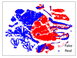
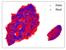
Multi-class Classification. Credit and Cabs are multi-class classification datasets, for which it is challenging to synthesize. For Credit in Table 4, IT-GAN(Q) shows the best performance in terms of Macro F1 and ROCAUC, and TVAE shows the best Micro F1 score. This is caused by the class imbalance problem where the minor class occupies a portion of 9%. TVAE doesn’t create any records for it and achieves the best Micro F1 score. Therefore, IT-GAN(Q) is the best in Credit. In Figure 4 in Appendix B, IT-GAN(L) actively synthesizes fake records that are not overlapped with real records, which results in sub-optimal outcomes.
For Cabs in Table 4, IT-GAN(Q) shows the best scores in terms of Micro/Macro F1. Interestingly, IT-GAN(L) has the second best scores. From this, we can know that the sacrifice caused by increasing the negative log-density is not too much in this dataset.
| Method | Ex. Var. | MSE | MAE | |
| Real | 0.50±0.11 | 0.61±0.02 | 0.14±0.03 | 0.30±0.03 |
| TVAE | 0.44±0.01 | 0.52±0.04 | 0.16±0.00 | 0.32±0.01 |
| TGAN | 0.43±0.01 | 0.60±0.00 | 0.16±0.00 | 0.32±0.00 |
| TableGAN | 0.41±0.02 | 0.46±0.03 | 0.17±0.01 | 0.33±0.01 |
| VeeGAN | 0.25±0.15 | 0.32±0.14 | 0.21±0.04 | 0.37±0.03 |
| IT-GAN(Q) | 0.59±0.00 | 0.60±0.00 | 0.12±0.00 | 0.28±0.00 |
| IT-GAN(L) | 0.53±0.01 | 0.56±0.01 | 0.13±0.00 | 0.29±0.00 |
| IT-GAN | 0.59±0.01 | 0.60±0.01 | 0.12±0.00 | 0.27±0.00 |
| Method | Ex.Var | MSE | MAE | ||
| Real | 0.15±0.01 | 0.15±0.00 | 0.69± 0.00 | 0.63±0.01 | |
| TVAE | -0.09±0.03 | 0.03±0.04 | 0.88±0.03 | 0.67±0.01 | |
| TGAN | 0.06±0.02 | 0.07±0.01 | 0.76±0.01 | 0.66±0.02 | |
| IT-GAN(Q) | 0.09±0.01 | 0.09±0.01 | 0.74±0.01 | 0.65±0.01 | |
| IT-GAN(L) | 0.03±0.03 | 0.06±0.02 | 0.78±0.03 | 0.65±0.01 | |
| IT-GAN | 0.09±0.02 | 0.10±0.01 | 0.74±0.01 | 0.64±0.00 |
Regression. King and News are regression datasets. Many methods show poor qualities in these datasets and tasks, and we removed them from Tables 6 and 6. In particular, all methods except TGAN, IT-GAN and its variations show negative scores for in News. Only our methods show reliable syntheses in all metrics. For King, our method and TGAN show good performance, but IT-GAN(Q) outperforms all baselines for almost all metrics.

| Model | Adult | Census | Credit | Cabs | King | News |
|---|---|---|---|---|---|---|
| IT-GAN(Q) | 0.612±0.008 | 0.833±0.011 | 0.710±0.012 | 0.659±0.016 | 0.761±0.025 | 0.791±0.003 |
| IT-GAN(L) | 0.599±0.016 | 0.741±0.027 | 0.656±0.027 | 0.630±0.011 | 0.703±0.032 | 0.783±0.010 |
| IT-GAN | 0.618±0.003 | 0.816±0.019 | 0.688±0.058 | 0.654±0.033 | 0.742±0.003 | 0.788±0.007 |
| Ex.Var | MSE | MAE | ||
|---|---|---|---|---|
| 32 | 0.00 | 0.01 | 0.80 | 0.67 |
| 64 | 0.03 | 0.05 | 0.78 | 0.66 |
| 128 | 0.06 | 0.07 | 0.76 | 0.65 |
| Ex.Var | MSE | MAE | ||
|---|---|---|---|---|
| -0.0105 | 0.05 | 0.07 | 0.77 | 0.66 |
| -0.0100 | 0.06 | 0.07 | 0.76 | 0.65 |
| 0.0000 | 0.07 | 0.10 | 0.75 | 0.64 |
| 0.0100 | 0.10 | 0.11 | 0.73 | 0.64 |
| 0.0500 | 0.10 | 0.10 | 0.73 | 0.65 |
| FBB ROCAUC | |
|---|---|
| -0.012 | 0.762 |
| -0.011 | 0.752 |
| 0.000 | 0.784 |
| 0.050 | 0.787 |
| 0.100 | 0.792 |
Privacy Attack. In [5], a full black-box privacy attack method to GANs has been proposed. We implemented their method to attack our method and measure the attack success score in terms of ROCAUC. In Table 7, we report the full black-box attack success scores for our method only. Refer to Appendix G for more detailed results. In most of the cases, IT-GAN(L) shows the lowest attack success score. This specific IT-GAN(L) is the one we used to report the performance in other tables. Note that IT-GAN(L) shows good performance for classification and regression while having the lowest attack success score.
Ablation Study on Negative Log-Density. We compare IT-GAN and its variations. IT-GAN(Q) outperforms IT-GAN in Adult, Census, Credit, Cabs, and King. According to these, we can conclude that decreasing the negative log-density improves task-oriented evaluation metrics.
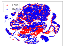
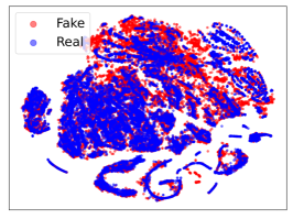
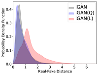
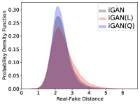
In Figure 3, we show the density function of the real-fake distance in various datasets whereas their mean values are shown in other experimental result tables. IT-GAN(L) effectively regularizes the distance. IT-GAN(Q) shows more similar distributions than IT-GAN. Therefore, we can know that controlling the negative log-density works as intended. The visualization in Figure 1 also proves it.
Sensitivity Analyses. By changing the two key hyperparameters and in our methods, we also conduct sensitivity analyses. We test IT-GAN(L) with various settings for . In general, produces the best result as shown in Table 10. With IT-GAN in Table 10, we variate , and produces many good outcomes. In Table 10, is robust to the full black-box attack. We refer to Appendix F for other tables.
5 Conclusions
We tackled the problem of synthesizing tabular data with the adversarial training of GANs and the negative log-density regularization of invertible neural networks. Our experimental results show that the proposed methods work well in most cases and the negative log-density regularization can adjust the trade-off between the synthesis quality and the robustness to the privacy attack. However, we found that some datasets are challenging to synthesize, i.e., all generative models show lower performance than Real in some multi-class and/or imbalanced datasets, e.g., Census and Credit. In addition, the best performing method varies from one dataset/task to another, and there still exists a room to improve qualities for them.
Societal Impacts & Limitations Our research will foster more actively sharing and releasing tabular data. One can use our method to synthesize fake data but it is unclear how the adversary can benefit from our research. At the same time, however, there exists a room to improve the quality of tabular data synthesis. It is still under-explored whether fake tabular data can be used for general machine learning tasks (although we showed that they can be used for classification and regression).
Acknowledgements
Jaehoon Lee and Jihyeon Hyeong equally contributed. Noseong Park is the corresponding author. This work was supported by the Institute of Information & Communications Technology Planning & Evaluation (IITP) grant funded by the Korean government (MSIT) (No. 2020-0-01361, Artificial Intelligence Graduate School Program (Yonsei University)).
References
- Adler & Lunz [2018] Adler, J. and Lunz, S. Banach wasserstein gan. In NeurIPS. 2018.
- Arjovsky et al. [2017] Arjovsky, M., Chintala, S., and Bottou, L. Wasserstein generative adversarial networks. In ICML, 2017.
- Aviñó et al. [2018] Aviñó, L., Ruffini, M., and Gavaldà, R. Generating synthetic but plausible healthcare record datasets, 2018.
- Che et al. [2017] Che, Z., Cheng, Y., Zhai, S., Sun, Z., and Liu, Y. Boosting deep learning risk prediction with generative adversarial networks for electronic health records. 2017.
- Chen et al. [2020] Chen, D., Yu, N., Zhang, Y., and Fritz, M. Gan-leaks: A taxonomy of membership inference attacks against generative models. In CCS, 2020.
- Chen et al. [2018] Chen, R. T. Q., Rubanova, Y., Bettencourt, J., and Duvenaud, D. K. Neural ordinary differential equations. In NeurIPS. 2018.
- Choi et al. [2017] Choi, E., Biswal, S., Maline, A. B., Duke, J., Stewart, F. W., and Sun, J. Generating multi-label discrete electronic health records using generative adversarial networks. 2017.
- Chow & Liu [1968] Chow, C. and Liu, C. Approximating discrete probability distributions with dependence trees. IEEE Transactions on Information Theory, 14(3):462–467, 1968.
- Cormode et al. [2011] Cormode, G., Procopiuc, M., Shen, E., Srivastava, D., and Yu, T. Differentially private spatial decompositions. 2011.
- Dinh et al. [2015] Dinh, L., Krueger, D., and Bengio, Y. NICE: non-linear independent components estimation. In ICLR, 2015.
- Dinh et al. [2017] Dinh, L., Sohl-Dickstein, J., and Bengio, S. Density estimation using real NVP. In ICLR, 2017.
- Dormand & Prince [1980] Dormand, J. and Prince, P. A family of embedded runge-kutta formulae. Journal of Computational and Applied Mathematics, 6(1):19 – 26, 1980.
- Esteban et al. [2017] Esteban, C., Hyland, L. S., and Rätsch, G. Real-valued (medical) time series generation with recurrent conditional gans, 2017.
- FOLLAND [1995] FOLLAND, G. B. Introduction to Partial Differential Equations: Second Edition, volume 102. Princeton University Press, 1995.
- Goodfellow et al. [2014] Goodfellow, I., Pouget-Abadie, J., Mirza, M., Xu, B., Warde-Farley, D., Ozair, S., Courville, A., and Bengio, Y. Generative adversarial nets. In NeurIPS. 2014.
- Grathwohl et al. [2019] Grathwohl, W., Chen, R. T. Q., Bettencourt, J., Sutskever, I., and Duvenaud, D. Ffjord: Free-form continuous dynamics for scalable reversible generative models. In ICLR, 2019.
- Grover et al. [2018] Grover, A., Dhar, M., and Ermon, S. Flow-gan: Combining maximum likelihood and adversarial learning in generative models. In AAAI, 2018.
- Gulrajani et al. [2017] Gulrajani, I., Ahmed, F., Arjovsky, M., Dumoulin, V., and Courville, A. Improved training of wasserstein gans. In NeurIPS, 2017.
- Hutchinson [1990] Hutchinson, M. A stochastic estimator of the trace of the influence matrix for laplacian smoothing splines. Communications in Statistics - Simulation and Computation, 19(2), 1990.
- Ishfaq et al. [2018] Ishfaq, H., Hoogi, A., and Rubin, D. Tvae: Triplet-based variational autoencoder using metric learning, 2018.
- Jordon et al. [2019] Jordon, J., Yoon, J., and Schaar, V. D. M. Pate-gan: Generating synthetic data with differential privacy guarantees. In International Conference on Learning Representations, 2019.
- Kelwin Fernandes [2015] Kelwin Fernandes. Online News Popularity Data Set. https://archive.ics.uci.edu/ml/datasets/Twenty+Newsgroups, 2015.
- King County [2021] King County. House Sales in King County, USA. https://www.kaggle.com/harlfoxem/housesalesprediction, 2021.
- Kingma & Welling [2014] Kingma, D. P. and Welling, M. Auto-encoding variational bayes. In ICLR, 2014.
- Kingma et al. [2016] Kingma, D. P., Salimans, T., Jozefowicz, R., Chen, X., Sutskever, I., and Welling, M. Improved variational inference with inverse autoregressive flow. In NeurIPS, 2016.
- Oliva et al. [2018] Oliva, J., Dubey, A., Zaheer, M., Poczos, B., Salakhutdinov, R., Xing, E., and Schneider, J. Transformation autoregressive networks. In ICML, 2018.
- Park et al. [2018] Park, N., Mohammadi, M., Gorde, K., Jajodia, S., Park, H., and Kim, Y. Data synthesis based on generative adversarial networks. 2018.
- Patel et al. [2018] Patel, S., Kakadiya, A., Mehta, M., Derasari, R., Patel, R., and Gandhi, R. Correlated discrete data generation using adversarial training. 2018.
- Patki et al. [2016] Patki, N., Wedge, R., and Veeramachaneni, K. The synthetic data vault. In DSAA, 2016.
- Reiter [2005] Reiter, P. J. Using cart to generate partially synthetic, public use microdata. Journal of Official Statistics, 21:441, 01 2005.
- Rezende & Mohamed [2015] Rezende, D. and Mohamed, S. Variational inference with normalizing flows. volume 37 of Proceedings of Machine Learning Research, pp. 1530–1538, 2015.
- Ronny Kohavi [1996a] Ronny Kohavi. Adult Data Set. http://archive.ics.uci.edu/ml/datasets/adult, 1996a.
- Ronny Kohavi [1996b] Ronny Kohavi. Census Income Data Set. https://archive.ics.uci.edu/ml/datasets/census+income, 1996b.
- Sigma Cabs [2021] Sigma Cabs. Trip Pricing with Taxi Mobility Analytics. https://www.kaggle.com/arashnic/taxi-pricing-with-mobility-analytics, 2021.
- Srivastava et al. [2017] Srivastava, A., Valkov, L., Russell, C., Gutmann, M. U., and Sutton, C. Veegan: Reducing mode collapse in gans using implicit variational learning. In NeurIPS. 2017.
- van den Berg et al. [2018] van den Berg, R., Hasenclever, L., Tomczak, J., and Welling, M. Sylvester normalizing flows for variational inference. In UAI, 2018.
- van der Maaten & Hinton [2008] van der Maaten, L. and Hinton, G. Visualizing data using t-sne. Journal of Machine Learning Research, 9(86), 2008.
- Xu et al. [2019] Xu, L., Skoularidou, M., Cuesta-Infante, A., and Veeramachaneni, K. Modeling tabular data using conditional gan. In NeurIPS. 2019.
- Yoon et al. [2019] Yoon, J., Jarrett, D., and van der Schaar, M. Time-series generative adversarial networks. In NeurIPS, 2019.
- Zaur Begiev [2017] Zaur Begiev. Bank Loan Status Dataset. https://www.kaggle.com/zaurbegiev/my-dataset?select=credit_train.csv, 2017.
- Zhang et al. [2016] Zhang, J., Xiao, X., and Xie, X. Privtree: A differentially private algorithm for hierarchical decompositions. 2016.
- Zhang et al. [2017] Zhang, J., Cormode, G., Procopiuc, C. M., Srivastava, D., and Xiao, X. Privbayes: Private data release via bayesian networks. ACM Transactions on Database Systems, 2017.
Appendix A Datasets
We summarize the statistics of our datasets as follows:
-
1.
Adult has 22K training, 10K testing records with 6 continuous numerical, 8 categorical, and 1 discrete numerical columns.
-
2.
Census has 200K training, 100K testing records with 7 continuous numerical, 34 categorical, and 0 discrete numerical columns.
-
3.
Credit has 30K training records, 5K testing records with 13 continuous numerical, 4 categorical, and 0 discrete numerical columns.
-
4.
Cabs has 40K training records, 5K testing records with 8 continuous numerical, 5 categorical, and 0 discrete numerical columns.
-
5.
King has 16K training records, 5K testing records with 14 continuous numerical, 2 categorical, and 0 discrete numerical columns.
-
6.
News has 32K training records, 8K testing records with 45 continuous numerical, 14 categorical, and 0 discrete numerical columns.
Appendix B Additional Synthesis Visualization
We introduce one more visualization with Credit in Figure 4. IT-GAN(Q) shows the best similarity between the real and fake points.
Appendix C Baseline Methods
We compare our method with the following baseline methods, including state-of-the-art VAEs and GANs for tabular data synthesis and our IT-GAN’s three variations:
-
1.
Ind is a heuristic method that we independently sample a value from each column’s ground-truth distribution.
-
2.
Uniform is to independently sample a value from a uniform distribution for each column, where and means the min and max value of the column.
-
3.
CLBN [8] is a Bayesian network built by the Chow-Liu algorithm representing a joint probability distribution.
-
4.
PrivBN [42] is a differentially private method for synthesizing tabular data using Bayesian networks.
-
5.
MedGAN [7] is a GAN that generates discrete medical records by incorporating non-adversarial losses.
-
6.
VeeGAN [35] is a GAN that generates tabular data with an additional reconstructor network to avoid mode collapse.
-
7.
TableGAN [27] is a GAN that generates tabular data using convolutional neural networks.
-
8.
TVAE [20] is a variational autoencoder (VAE) model to generate tabular data.
-
9.
TGAN [38] is a GAN that generates tabular data with mixed types of variables. We use these baselines’ hyperparameters recommended in their original paper and/or GitHub repositories.
Appendix D Best Hyperparameters for Reproducibility
We list the best hyperparameter configurations for our methods in each dataset. In all cases, we observed the best performance with mini-batch size of 2,000, and size of 128.
-
1.
Adult,
-
•
For IT-GAN(Q),
-
•
For IT-GAN(L),
-
•
For IT-GAN,
-
•
-
2.
Census,
-
•
For IT-GAN(Q),
-
•
For IT-GAN(L),
-
•
For IT-GAN,
-
•
-
3.
Credit,
-
•
For IT-GAN(Q),
-
•
For IT-GAN(L),
-
•
For IT-GAN,
-
•
-
4.
Cabs,
-
•
For IT-GAN(Q),
-
•
For IT-GAN(L),
-
•
For IT-GAN,
-
•
-
5.
King,
-
•
For IT-GAN(Q),
-
•
For IT-GAN(L),
-
•
For IT-GAN,
-
•
-
6.
News,
-
•
For IT-GAN(Q),
-
•
For IT-GAN(L),
-
•
For IT-GAN,
-
•
Appendix E Full Experimental Results
Appendix F Parameter Sensitivity Analyses
Appendix G Experimental Evaluations with Privacy Attacks
We attack our method using the method in [5]. Chen et al. proposed an efficient and effective method, given a GAN model, to infer whether a record belongs to its original training data. In their research, the following full black-box attack model was actively studied because it most frequently occurs in real-world environments for releasing/sharing tabular data.
In the full black-box (FBB) attack, the attacker can access only to fake tabular data generated by its victim model . Given an unknown record in hand, the attacker approximates the probability that it is a member of the real tabular data used to train , i.e., . The attacker uses the nearest neighbor to among as its reconstructed copy , and calculates a reconstruction error (e.g., Euclidean distance) between and . The idea behind the method is that if the record actually belongs to the real tabular data , then it will be better reconstructed with a smaller error.
Using the FBB method, we attack IT-GAN, IT-GAN(Q), IT-GAN(L), and several sub-optimal versions of IT-GAN to compare the attack success scores for them. The reason why we include the sub-optimal versions of IT-GAN is that one can easily decrease the attack success score by selecting sub-optimal models (and thereby, potentially sacrificing the synthesis quality). We show that IT-GAN(L) is a more principled way to trade off between the two factors. Also, since the attacker is more likely to target high-quality models, we selectively attack TGAN and TVAE, which show comparably high synthesis quality in some cases.
To evaluate the attack success scores, we create a balanced evaluation set of the randomly-sampled training data and the original testing data from Adult, Census, and so on. If an attack correctly classifies random training samples as the original training data and testing samples as not belonging to it, it turns out to be successful. As this attack is a binary classification, we use the ROCAUC score as its evaluation metric. We train, generate and attack each generative model for five times with different seed numbers and report the average and std. dev. of their attack success scores.
As shown in Table 25, IT-GAN(L) shows the lowest attack success scores overall. For Cabs and Credit, the attack success scores of TVAE are the lowest among all methods, which means it is the most robust to the attack among all the methods for those two datasets. However, it marks relatively poor synthesis quality for them as reported in Tables 4 and 4. IT-GAN(L) shows attack success scores close to those of TVAE while it shows better machine learning tasks scores, e.g., a Macro F1 score of 0.60 by TVAE vs. 0.66 by IT-GAN(L) in Cabs. All in all, TVAE shows its robustness in the two datasets for its relatively low synthesis quality but in general, IT-GAN(L) achieves the best trade-off between synthesis quality and privacy protection.
We also compare with various sub-optimal versions of IT-GAN. While training IT-GAN, we could obtain several sub-optimal versions around the epoch where we obtain IT-GAN and call them as IT-GAN(S) with . They all show sub-optimal accuracy in comparison with IT-GAN. One easy way to protect sensitive information in the original data is to use these sub-optimal versions. These IT-GAN(S) sub-optimal models have F1 (resp. MSE) scores worse (resp. larger) than those of IT-GAN in Tables 2 to 6 by — if multiple sub-optimal models have the same score, we choose the sub-optimal model with the largest distance to increase the robustness to the attack. However, they typically fail to obtain a good trade-off between synthesis quality and information protection. Among those three sub-optimal versions, for instance, IT-GAN(S1) shows the best synthesis quality. However, IT-GAN(L) still outperforms it in 5 out of the 6 datasets in terms of the task-oriented evaluation metrics in Tables 2 to 6. Therefore, we can say that IT-GAN(L) is a more principled method than other methods in terms of the trade-off. IT-GAN(L) is able to synthesize high-quality fake records while successfully regularizing the log-density of real records.
In the following two tables (Tables 25 and 25), we show the sensitivity analyses related to the attack. By increasing or decreasing , our model’s robustness can be properly adjusted as expected. This property is our main research goal in this paper. Our framework, which combines the adversarial training and the negative log-density regularization, provides a principled way for synthesizing tabular data.
| Method | Acc. | F1 | ROCAUC | EMD |
| Real | 0.83±0.00 | 0.66±0.00 | 0.88±0.00 | 0.00±0.00 |
| CLBN | 0.77±0.00 | 0.31±0.03 | 0.78±0.01 | 2.05e+03±10.28 |
| Ind | 0.65±0.03 | 0.17±0.04 | 0.51±0.08 | 27.88±2.9 |
| PrivBN | 0.79±0.01 | 0.43±0.02 | 0.84±0.01 | 3.15e+02±14.82 |
| Uniform | 0.49±0.10 | 0.26±0.09 | 0.50± 0.07 | 6.42e+03±19.13 |
| TVAE | 0.81±0.00 | 0.62±0.01 | 0.84±0.01 | 6.28e+02±1.08e+02 |
| TGAN | 0.81±0.00 | 0.63±0.01 | 0.85±0.01 | 2.22e+02±1.71e+02 |
| TableGAN | 0.80±0.01 | 0.46±0.03 | 0.81±0.01 | 1.07e+02±13.52 |
| VeeGAN | 0.69±0.04 | 0.47±0.04 | 0.73±0.04 | 1.78e+03±1.57e+02 |
| MedGAN | 0.71±0.05 | 0.48±0.05 | 0.74±0.02 | 7.06e+03±1.53e+02 |
| IT-GAN(Q) | 0.81±0.00 | 0.64±0.01 | 0.86±0.00 | 87.32±42.34 |
| IT-GAN(L) | 0.80±0.01 | 0.64±0.01 | 0.85±0.01 | 3.21e+02±72.21 |
| IT-GAN | 0.81±0.00 | 0.64±0.01 | 0.86±0.01 | 72.49±6.36 |
| Method | Acc. | F1 | ROCAUC | EMD |
| Real | 0.91±0.00 | 0.47±0.01 | 0.90± 0.00 | 0.00±0.00 |
| CLBN | 0.90± 0.00 | 0.29±0.01 | 0.75±0.01 | 15.07±0.03 |
| Ind | 0.71±0.05 | 0.06±0.01 | 0.45±0.02 | 0.13±0.01 |
| PrivBN | 0.91±0.01 | 0.23±0.03 | 0.81±0.03 | 5.64±1.78 |
| Uniform | 0.49±0.22 | 0.11±0.01 | 0.48±0.05 | 2.08e+02±0.12 |
| TVAE | 0.93±0.00 | 0.44±0.01 | 0.86±0.01 | 1.09±0.15 |
| TGAN | 0.91±0.01 | 0.38±0.03 | 0.86±0.02 | 0.98±0.08 |
| TableGAN | 0.93±0.01 | 0.31±0.06 | 0.81±0.03 | 0.81±0.22 |
| VeeGAN | 0.85±0.07 | 0.18±0.08 | 0.67±0.08 | 1.57±0.03 |
| MedGAN | 0.78±0.13 | 0.15±0.06 | 0.64±0.09 | 2.38e+02±46.19 |
| IT-GAN(Q) | 0.91±0.00 | 0.45±0.01 | 0.89±0.00 | 1.02±0.09 |
| IT-GAN(L) | 0.91±0.01 | 0.46±0.01 | 0.88±0.01 | 3.77±1.25 |
| IT-GAN | 0.91±0.00 | 0.45±0.01 | 0.88±0.00 | 1.29±0.31 |
| Method | Acc. | Macro F1 | Micro F1 | ROCAUC | EMD |
| Real | 0.61±0.00 | 0.48±0.01 | 0.61±0.00 | 0.67±0.00 | 0.00±0.00 |
| CLBN | 0.48±0.01 | 0.34±0.02 | 0.48±0.01 | 0.56±0.01 | 1.85e+06±4.40e+03 |
| Ind | 0.44±0.01 | 0.27±0.01 | 0.44±0.01 | 0.51±0.01 | 1.13e+04±5.51e+03 |
| PrivBN | 0.51±0.01 | 0.32±0.02 | 0.51±0.01 | 0.60±0.00 | 3.93e+05±3.85e+04 |
| Uniform | 0.34±0.07 | 0.24±0.04 | 0.34±0.07 | 0.50±0.02 | 1.89e+07±4.20e+04 |
| TVAE | 0.57±0.00 | 0.39±0.00 | 0.57±0.00 | 0.58±0.00 | 4.65e+05±1.01e+05 |
| TGAN | 0.55±0.01 | 0.40±0.00 | 0.55±0.01 | 0.59±0.00 | 2.36e+05±1.95e+05 |
| TableGAN | 0.47±0.02 | 0.35±0.01 | 0.47±0.02 | 0.54±0.01 | 2.08e+05±2.30e+04 |
| VeeGAN | 0.48±0.03 | 0.36±0.02 | 0.48±0.03 | 0.54±0.02 | 1.85e+06±4.31e+05 |
| MedGAN | 0.51±0.03 | 0.37±0.02 | 0.51±0.03 | 0.56±0.01 | 1.95e+07±2.22e+06 |
| IT-GAN(Q) | 0.54±0.01 | 0.41±0.01 | 0.54±0.01 | 0.60±0.00 | 3.62e+05±2.15e+05 |
| IT-GAN(L) | 0.55±0.01 | 0.40±0.01 | 0.55±0.01 | 0.60±0.01 | 5.29e+05±3.00e+05 |
| IT-GAN | 0.54±0.01 | 0.40±0.00 | 0.54±0.01 | 0.59±0.01 | 2.38e+05±1.12e+05 |
| Method | Acc. | Macro F1 | Micro F1 | ROCAUC | EMD |
| Real | 0.68±0.00 | 0.65±0.00 | 0.68±0.00 | 0.78±0.00 | 0.00±0.00 |
| CLBN | 0.66±0.00 | 0.63±0.00 | 0.66±0.00 | 0.76±0.00 | 6.72±0.0 |
| Ind | 0.39±0.01 | 0.31±0.01 | 0.39±0.01 | 0.50± 0.01 | 0.05±0.0 |
| PrivBN | 0.67±0.00 | 0.64±0.00 | 0.67±0.00 | 0.77±0.00 | 0.25±0.0 |
| Uniform | 0.31±0.02 | 0.28±0.02 | 0.31±0.02 | 0.47±0.02 | 3.64±0.02 |
| TVAE | 0.66±0.01 | 0.60± 0.02 | 0.66±0.01 | 0.74±0.01 | 0.66±0.13 |
| TGAN | 0.67±0.00 | 0.64±0.00 | 0.67±0.00 | 0.76±0.00 | 0.38±0.11 |
| TableGAN | 0.41±0.02 | 0.35±0.03 | 0.41±0.02 | 0.52±0.03 | 0.21±0.06 |
| VeeGAN | 0.60± 0.05 | 0.54±0.06 | 0.60± 0.05 | 0.71±0.02 | 2.02±0.64 |
| MedGAN | 0.55±0.03 | 0.48±0.03 | 0.55±0.03 | 0.65±0.02 | 4.56±0.17 |
| IT-GAN(Q) | 0.69±0.00 | 0.66±0.00 | 0.69±0.00 | 0.79±0.01 | 0.33±0.10 |
| IT-GAN(L) | 0.68±0.01 | 0.66±0.01 | 0.68±0.01 | 0.79±0.00 | 0.63±0.11 |
| IT-GAN | 0.67±0.01 | 0.64±0.01 | 0.67±0.01 | 0.77±0.00 | 0.36±0.09 |
| Method | Ex.Var | MSE | MAE | EMD | |
| Real | 0.50±0.11 | 0.61±0.02 | 0.14±0.03 | 0.30±0.03 | 0.00±0.00 |
| CLBN | -0.05±0.29 | 0.35±0.06 | 0.57±0.40 | 0.56±0.21 | 3.53e+04±1.60e+02 |
| Ind | -0.09±0.26 | 0.13±0.04 | 0.34±0.14 | 0.46±0.10 | 5.35e+02±51.97 |
| PrivBN | -0.01±0.20 | 0.51±0.02 | 0.31±0.09 | 0.44±0.07 | 1.30e+04±1.23e+03 |
| Uniform | -0.98±0.05 | 0.05±0.05 | 3.84±2.13 | 1.76±0.57 | 2.55e+05±1.23e+03 |
| TVAE | 0.44±0.01 | 0.52±0.04 | 0.16±0.00 | 0.32±0.01 | 2.65e+03±3.97e+02 |
| TGAN | 0.43±0.01 | 0.60± 0.00 | 0.16±0.00 | 0.32±0.00 | 5.67e+03±2.20e+03 |
| TableGAN | 0.41±0.02 | 0.46±0.03 | 0.17±0.01 | 0.33±0.01 | 3.62e+03±3.51e+02 |
| VeeGAN | 0.25±0.15 | 0.32±0.14 | 0.21±0.04 | 0.37±0.03 | 6.83e+04±5.32e+04 |
| MedGAN | -0.39±0.02 | 0.01±0.13 | 0.97±0.19 | 0.78±0.08 | 2.90e+05±3.09e+04 |
| IT-GAN(Q) | 0.59±0.00 | 0.60±0.00 | 0.12±0.00 | 0.28±0.00 | 2.04e+03±2.66e+02 |
| IT-GAN(L) | 0.53±0.01 | 0.56±0.02 | 0.13±0.00 | 0.29±0.00 | 1.63e+04±6.17e+03 |
| IT-GAN | 0.59±0.01 | 0.60±0.01 | 0.12±0.00 | 0.27±0.00 | 4.57e+03±1.27e+03 |
| Method | Ex.Var | MSE | MAE | EMD | |
| Real | 0.15±0.01 | 0.15±0.00 | 0.69± 0.00 | 0.63±0.01 | 0.00±0.00 |
| CLBN | -1.00±0.00 | -1.08±0.56 | 5.75±0.95 | 1.99±0.18 | 1.60e+04±23.41 |
| Ind | -0.06±0.05 | -0.03±0.03 | 0.85±0.04 | 0.70± 0.01 | 1.07e+02±12.39 |
| PrivBN | -0.58±0.12 | -1.04±0.67 | 1.93±0.61 | 1.04±0.10 | 1.04e+03±18.63 |
| Uniform | -0.86±0.17 | -1.02±1.43 | 4.73±1.41 | 1.79±0.21 | 3.98e+04±28.96 |
| TVAE | -0.09±0.03 | 0.03±0.04 | 0.88±0.03 | 0.67±0.01 | 8.74e+02±1.88e+02 |
| TGAN | 0.06±0.02 | 0.07±0.01 | 0.76±0.01 | 0.66±0.02 | 4.99e+02±94.4 |
| TableGAN | -0.86±0.09 | -0.80±0.30 | 1.61±0.16 | 1.01±0.04 | 1.21e+03±3.84e+02 |
| VeeGAN | -0.91±0.15 | -1.36e+07±2.49e+07 | 1.49e+07±2.83e+07 | 9.54e+02±1.35e+03 | 4.63e+03±8.00e+02 |
| MedGAN | -0.73±0.08 | -0.19±0.08 | 3.99±0.06 | 1.64±0.03 | 3.93e+04±4.06e+03 |
| IT-GAN(Q) | 0.09±0.01 | 0.09±0.01 | 0.74±0.01 | 0.65±0.01 | 2.24e+02±62.01 |
| IT-GAN(L) | 0.03±0.03 | 0.06±0.02 | 0.78±0.03 | 0.65±0.01 | 1.02e+03±98.7 |
| IT-GAN | 0.09±0.02 | 0.10±0.01 | 0.74±0.01 | 0.64±0.00 | 4.86e+02±1.21e+02 |
| Acc. | F1 | ROCAUC | EMD | |
|---|---|---|---|---|
| 32 | 0.81 | 0.64 | 0.85 | 108.71 |
| 64 | 0.81 | 0.65 | 0.86 | 67.07 |
| 128 | 0.80 | 0.65 | 0.86 | 231.45 |
| Acc. | F1 | ROCAUC | EMD | |
|---|---|---|---|---|
| 32 | 0.91 | 0.42 | 0.87 | 1.34 |
| 64 | 0.90 | 0.46 | 0.89 | 1.17 |
| 128 | 0.91 | 0.47 | 0.89 | 3.34 |
| Ex.Var | MSE | MAE | EMD | ||
|---|---|---|---|---|---|
| 32 | 0.00 | 0.01 | 0.80 | 0.67 | 1270.44 |
| 64 | 0.03 | 0.05 | 0.78 | 0.66 | 302.38 |
| 128 | 0.06 | 0.07 | 0.76 | 0.65 | 972.37 |
| Acc. | F1 | ROCAUC | EMD | |
|---|---|---|---|---|
| -0.018 | 0.79 | 0.64 | 0.85 | 377.11 |
| -0.014 | 0.80 | 0.65 | 0.86 | 231.45 |
| -0.010 | 0.80 | 0.64 | 0.86 | 169.16 |
| 0.000 | 0.81 | 0.64 | 0.86 | 76.13 |
| 0.010 | 0.81 | 0.65 | 0.86 | 92.04 |
| 0.050 | 0.81 | 0.65 | 0.86 | 83.74 |
| 0.100 | 0.81 | 0.64 | 0.86 | 167.99 |
| Acc. | F1 | ROCAUC | EMD | |
|---|---|---|---|---|
| -0.20 | 0.90 | 0.43 | 0.87 | 0.89 |
| -0.10 | 0.91 | 0.47 | 0.89 | 3.34 |
| -0.05 | 0.91 | 0.45 | 0.88 | 1.15 |
| 0.00 | 0.91 | 0.46 | 0.89 | 1.73 |
| 0.05 | 0.90 | 0.44 | 0.88 | 0.83 |
| 0.10 | 0.90 | 0.44 | 0.89 | 0.84 |
| 0.50 | 0.90 | 0.46 | 0.89 | 2.91 |
| Ex.Var | MSE | MAE | EMD | ||
|---|---|---|---|---|---|
| -0.0120 | -0.06 | 0.03 | 0.85 | 0.67 | 1252.72 |
| -0.0110 | 0.02 | 0.07 | 0.79 | 0.65 | 1192.79 |
| -0.0105 | 0.05 | 0.07 | 0.77 | 0.66 | 1009.46 |
| -0.0100 | 0.06 | 0.07 | 0.76 | 0.65 | 972.37 |
| 0.000 | 0.07 | 0.10 | 0.75 | 0.64 | 620.97 |
| 0.0100 | 0.10 | 0.11 | 0.73 | 0.64 | 473.49 |
| 0.0500 | 0.10 | 0.10 | 0.73 | 0.65 | 320.15 |
| 0.1000 | 0.10 | 0.10 | 0.73 | 0.64 | 477.28 |
| Model | Adult | Census | Credit | Cabs | King | News |
|---|---|---|---|---|---|---|
| TVAE | 0.721±0.033 | 0.902±0.016 | 0.646±0.016 | 0.620±0.040 | 0.760±0.014 | 0.802±0.005 |
| TGAN | 0.647±0.012 | 0.848±0.014 | 0.684±0.023 | 0.688±0.011 | 0.781±0.007 | 0.799±0.004 |
| IT-GAN(Q) | 0.612±0.008 | 0.833±0.011 | 0.710±0.012 | 0.659±0.016 | 0.761±0.025 | 0.791±0.003 |
| IT-GAN(L) | 0.599±0.016 | 0.741±0.027 | 0.656±0.027 | 0.630±0.011 | 0.703±0.032 | 0.783±0.010 |
| IT-GAN | 0.618±0.003 | 0.816±0.019 | 0.688±0.058 | 0.654±0.033 | 0.742±0.003 | 0.788±0.007 |
| IT-GAN(S1) | 0.616±0.010 | 0.820±0.018 | 0.663±0.037 | 0.647±0.018 | 0.726±0.023 | 0.785±0.007 |
| IT-GAN(S2) | 0.614±0.006 | 0.829±0.023 | 0.664±0.039 | 0.643±0.033 | 0.711±0.025 | 0.784±0.008 |
| IT-GAN(S3) | 0.616±0.007 | 0.831±0.016 | 0.664±0.033 | 0.648±0.033 | 0.727±0.026 | 0.785±0.011 |
| FBB ROCAUC | |
|---|---|
| -0.018 | 0.583 |
| -0.014 | 0.605 |
| -0.01 | 0.606 |
| 0.0 | 0.623 |
| 0.01 | 0.614 |
| 0.05 | 0.621 |
| 0.1 | 0.610 |
| FBB ROCAUC | |
|---|---|
| -0.012 | 0.762 |
| -0.011 | 0.752 |
| -0.0105 | 0.783 |
| -0.01 | 0.774 |
| 0.0 | 0.784 |
| 0.01 | 0.781 |
| 0.05 | 0.787 |
| 0.1 | 0.792 |