On Unbalanced Optimal Transport: Gradient Methods, Sparsity and Approximation Error

Abstract

We study the Unbalanced Optimal Transport (UOT) between two measures of possibly different masses with at most $n$ components, where the marginal constraints of standard Optimal Transport (OT) are relaxed via Kullback-Leibler divergence with regularization factor $\tau$. Although only Sinkhorn-based UOT solvers have been analyzed in the literature with the iteration complexity of ${O}\big{(}\tfrac{\tau\log(n)}{\varepsilon}\log\big{(}\tfrac{\log(n)}{{\varepsilon}}\big{)}\big{)}$ and per-iteration cost of $O(n^{2})$ for achieving the desired error $\varepsilon$, their positively dense output transportation plans strongly hinder the practicality. On the other hand, while being vastly used as heuristics for computing UOT in modern deep learning applications and having shown success in sparse OT problem, gradient methods applied to UOT have not been formally studied. In this paper, we propose a novel algorithm based on Gradient Extrapolation Method (GEM-UOT) to find an $\varepsilon$-approximate solution to the UOT problem in $O\big{(}\kappa\log\big{(}\frac{\tau n}{\varepsilon}\big{)}\big{)}$ iterations with $\widetilde{O}(n^{2})$ per-iteration cost, where $\kappa$ is the condition number depending on only the two input measures. Our proof technique is based on a novel dual formulation of the squared $\ell_{2}$-norm UOT objective, which fills the lack of sparse UOT literature and also leads to a new characterization of approximation error between UOT and OT. To this end, we further present a novel approach of OT retrieval from UOT, which is based on GEM-UOT with fine tuned $\tau$ and a post-process projection step. Extensive experiments on synthetic and real datasets validate our theories and demonstrate the favorable performance of our methods in practice. We showcase GEM-UOT on the task of color transfer in terms of both the quality of the transfer image and the sparsity of the transportation plan.

Keywords: Unbalanced Optimal Transport; Gradient Methods; Convex Optimization

1 Introduction

The optimal transport (OT) problem originated from the need to find the optimal cost to transport masses from one distribution to another distribution (Villani, 2008). While initially developed by theorists, OT has found widespread applications in statistics and machine learning (ML) (see e.g. (Ho et al., 2017; Arjovsky et al., 2017; Rabin and Papadakis, 2015)). However, standard OT requires the restricted assumption that the input measures are normalized to unit mass, which facilitates the development of the Unbalanced Optimal Transport (UOT) problem between two measures of possibly different masses (Chizat et al., 2018). The class of UOT problem relaxes OT’s marginal constraints. Specifically, it is a regularized version of Kantorovich formulation placing penalty functions on the marginal distributions based on some given divergences (Liero et al., 2017). While there have been several divergences considered by the literature, such as squared $\ell_{2}$ norm (Blondel et al., 2018), $\ell_{1}$ norm (Caffarelli and McCann, 2010), or general $\ell_{p}$ norm (Lee et al., 2019), UOT with Kullback-Leiber (KL) divergence (Chizat et al., 2018) is the most prominent and has been used in statistics and machine learning (Frogner et al., 2015), deep learning (Yang and Uhler, 2019), domain adaptation (Balaji et al., 2020; Fatras et al., 2021), bioinformatics (Schiebinger et al., 2019), and OT robustness (Balaji et al., 2020; Le et al., 2021). Throughout this paper, we refer to UOT penalized by KL divergence as simply UOT, unless otherwise specified. We hereby define some notations and formally present our problem of interest.

Notations: We let $[n]$ stand for the set $\{1,2,...,n\}$ while $\mathbb{R}^{n}_{+}$ stands for the set of all vectors in $\mathbb{R}^{n}$ with nonnegative entries. For a vector $\mathbf{x}\in R^{n}$ and $p\in[1,\infty)$, we denote $\|\mathbf{x}\|_{p}$ as its $\ell_{p}$-norm and $diag(\mathbf{x})\in\mathbb{R}^{n\times n}$ as the diagonal matrix with $diag(\mathbf{x})_{ii}=x_{i}$. Let A and B be two matrices of size $n\times n$, we denote their Frobenius inner product as: $\left\langle A,B\right\rangle=\sum_{i,j=1}^{n}A_{ij}B_{ij}$. $\textbf{1}_{n}$ stands for a vector of length $n$ with all of its components equal to $1$. The KL divergence between two vectors $\mathbf{x},\mathbf{y}\in\mathbb{R}^{n}$ is defined as $\mathbf{KL}(x||y)=\sum_{i=1}^{n}x_{i}\log\left(\frac{x_{i}}{y_{i}}\right)-x_{i}+y_{i}$. The entropy of a matrix $X\in\mathbb{R}^{n\times n}_{+}$ is given by $H(X)=-\sum_{i,j=1}^{n}X_{ij}(\log(X_{ij})-1)$.

Unbalanced Optimal Transport: For a couple of finite measures with possibly different total mass $\mathbf{a}=(a_{1},...,a_{n})\in\mathbb{R}^{n}_{+}$ and $\mathbf{b}=(b_{1},...,b_{n})\in\mathbb{R}^{n}_{+}$, we denote $\alpha=\sum_{i=1}^{n}a_{i}$ and $\beta=\sum_{i=1}^{n}b_{i}$ as the total masses, and $a_{min}=\min_{1\leq i\leq n}\{a_{i}\}$ and $b_{min}=\min_{1\leq i\leq n}\{b_{i}\}$ as the minimum masses. The UOT problem can be written as:

$$\mathbf{UOT}_{\mathbf{KL}}(\mathbf{a}, \mathbf{b})=\min_{X\in\mathbb{R}_{+}^{n\times n}}\big{\{}f(X):=\left\langle C,X\right\rangle+\tau\mathbf{KL}(X\textbf{1}_{n}||\mathbf{a})+\tau\mathbf{KL}(X^{\top}\textbf{1}_{n}||\mathbf{b})\big{\}},$$ (1)

where $C$ is a given cost matrix, $X$ is a transportation plan, $\tau>0$ is a given regularization parameter. When $\mathbf{a}^{\top}\textbf{1}_{n}=\mathbf{b}^{\top}\textbf{1}_{n}$ and $\tau\rightarrow\infty$, (1) reduces to a standard OT problem. Let $X_{f}\in\mathop{\mathrm{argmin}}_{X\in\mathbb{R}_{+}^{n\times n}}f(X)$ be optimal transportation plan of the UOT problem (1).

Definition 1

For $\varepsilon>0$, $X$ is an $\varepsilon$-approximate transportation plan of $\mathbf{UOT}_{\mathbf{KL}}(\mathbf{a},\mathbf{b})$ if:

$$f(X)=\langle C,X\rangle+\tau\mathbf{KL}(X\textbf{1}_{n}||\mathbf{a})+\tau\mathbf{KL}(X^{\top}\textbf{1}_{n}||\mathbf{b})\leq\mathbf{UOT}_{\mathbf{KL}}(\mathbf{a},\mathbf{b})+\varepsilon.$$ (2)

1.1 Open Problems and Motivation

We hereby discuss the open problems within the UOT problem to better facilitate the motivation underpinning our work.

Nascent literature of gradient methods for UOT: While the existing work has well studied the class of OT problems using gradient methods or variations of the Sinkhorn algorithm (Guminov et al., 2021; Altschuler et al., 2017), the complexity theory and algorithms for UOT remain nascent despite its recent emergence. Pham et al. (2020) shows that Sinkhorn algorithm can solve the UOT problem in ${O}\big{(}\frac{\tau n^{2}\log(n)}{\varepsilon}\log\big{(}\frac{\log(n)}{\varepsilon}\big{)}\big{)}$ up to the desired error $\varepsilon$. Chapel et al. (2021) proposes Majorization-Minimization (MM) algorithm, which is Sinkhorn-based, as a numerical solver with $O(n^{3.27})$ empirical complexity. Thanks to their compatibility, gradient methods have been vastly used as heuristics for computing UOT in deep learning applications (Balaji et al., 2020; Yang and Uhler, 2019) and multi-label learning (Frogner et al., 2015). Nevertheless, no work has formally studied gradient methods applied to UOT problems. Principled study of this topic could lead to preliminary theoretical justification and guide the more refined design of gradient methods for UOT.

Lack of sparse UOT literature: There is currently no study of sparse UOT in the literature, which nullifies its usage in many applications (Pitié et al., 2007; Courty et al., 2017; Muzellec et al., 2016) in which only sparse transportation plan is of interest. On a side note, entropic regularization imposed by the Sinkhorn algorithm keeps the transportation plan dense and strictly positive (Essid and Solomon, 2018; Blondel et al., 2018).

Approximation of OT: The approximability of standard OT via UOT has remained an open problem. Recently, (Chapel et al., 2021) discusses the possibility to approximate OT transportation plan using that of UOT and empirically verifies it. Despite the well known fact that OT is recovered from UOT when $\tau\to\infty$ and the masses are balanced, no work has analyzed the rate under which UOT converges to OT. Characterization of approximation error between UOT and OT could give rise to the new perspective of OT retrieval from UOT, and facilitate further study of the UOT geometry and statistical bounds from the lens of OT (Bernton et al., 2022) in the regime of large $\tau$.

Bottleneck of robust OT computation via UOT: The UOT formulation with small $\tau$ has been vastly used as a robust variant of OT (Fatras et al., 2021; Balaji et al., 2020; Le et al., 2021). In this paper, we further highlight a major bottleneck of this approach having been neglected by the literature: though relaxing OT as UOT admits robustness to outliers, the computed UOT distance far deviates from the original OT distance. Under the naive choice of $\tau=1$ (Fatras et al., 2021; Balaji et al., 2020; Le et al., 2021), we observe that on CIFAR-10 as an example real dataset the UOT distance differs from OT by order of dozens (see Figure 14). Such large deviation from the original metric can be detrimental to target applications where the distance itself is of interest (Genevay et al., 2018). Another inherent limitation is that the solution returned by UOT is only a “relaxed” transportation plan that does not respect the marginal constraints of standard OT. This naturally raises the question whether despite the relaxation of OT as UOT, there is a way to retrieve the original OT distance and transportation plan.

1.2 Contributions

In this paper, we provide a comprehensive study of UOT that addresses all the aforementioned open problems and challenges of UOT literature. We consider the setting where KL divergences are used to penalize the marginal constraints. Our contributions can be summarized as follows:

• We provide a novel dual formulation of the squared $\ell_{2}$-norm regularized UOT objective, which is the basis of our algorithms. This could facilitate further algorithmic development for solving sparse or standard UOT, since the current literature is limited to the dual formulation of entropic-regularized UOT problem (Chizat et al., 2018).

• Based on the Gradient Extrapolation Method (GEM), we propose GEM-UOT algorithm for finding an $\varepsilon$-approximate solution to the UOT problem in $O\big{(}\kappa\log\big{(}\frac{\tau n}{\varepsilon}\big{)}\big{)}$ iterations with $\widetilde{O}(n^{2})$ per-iteration cost, where $\kappa$ is the condition number that depends on only the two input measures. Through GEM-UOT, we present the first i) principled study of gradient methods for UOT, ii) sparse UOT solver, and iii) algorithm that lifts the linear dependence on $\tau$ of Sinkhorn (Pham et al., 2020), a bottleneck in the regime of large $\tau$ (Sejourne et al., 2022).

• To the best of our knowledge, we establish the first characterization of the approximation error between UOT and OT (in the context of KL-penalized UOT). In particular, we show that both of UOT’s transportation plan and transport distance converge to OT’s marginal constraints and transport distance with the rate $O(\frac{poly(n)}{\tau})$. This result opens up directions that use UOT to approximate standard OT and accentuate the importance of our proposed GEM-UOT, which is the first to achieve logarithmic dependence on $\tau$ in the literature.

• Inspired by our results on approximation error, we bring up a new perspective of OT retrieval from UOT with fine-tuned $\tau$. In particular, we present GEM-OT, which obtains an $\varepsilon$-approximate solution to the standard OT problem by performing a post-process projection of UOT solution. GEM-OT is of order $\widetilde{O}(\kappa n^{2})$. While lots of work have naively relaxed OT into UOT to enjoy its unconstrained optimization structure and robustness to outliers, our results on $\tau$ make a further significant step by equipping such relaxation with provable guarantees.

Paper Organization: The rest of the paper is organized as follows. We introduce the background of regularized UOT problems and present our novel dual formulation in Section 2. In Section 3, we analyze the complexities our proposed algorithms GEM-UOT. The results on approximability of OT via UOT are established in Section  4. In Section 5, we experiment on both synthetic and real datasets to compare our algorithm with the state-of-the-art Sinkhorn algorithm in terms of both the performance and the induced sparsity, empirically verify our theories on approximation error, and showcase our framework on the task of color transfer. We conclude the paper in Section 6.

2 Background

In this Section, we first present the entropic regularized UOT problem, used by Sinkhorn algorithm. Then we consider the squared $\ell_{2}$-norm regularized UOT and derive a new dual formulation, which is the basis for our algorithmic design.

2.1 Entropic Regularized UOT

Inspired by the literature of the entropic regularized OT problem, the entropic version of the UOT problem has been considered. The problem is formulated as:

$$\min_{X\in\mathbb{R}_{+}^{n\times n}}\left\langle C,X\right\rangle-\eta H(X)+\tau\mathbf{KL}(X\textbf{1}_{n}||\mathbf{a})+\tau\mathbf{KL}(X^{\top}\textbf{1}_{n}||\mathbf{b}),$$ (3)

where $\eta>0$ is a given regularization parameter. By (Chizat et al., 2018), optimizing the Fenchel-Legendre dual of the above entropic regularized UOT is equivalent to:

$$\min_{\mathbf{u},\mathbf{v}\in\mathbb{R}^{n}}\eta\sum_{i,j=1}^{n}exp\bigg{(}\frac{u_{i}+v_{j}-C_{ij}}{\eta}\bigg{)}+\tau\left\langle e^{-\mathbf{u}/\tau},\mathbf{a}\right\rangle+\tau\left\langle e^{-\mathbf{v}/\tau},\mathbf{b}\right\rangle.$$ (4)

Remark 2

We note that existing algorithm (Pham et al., 2020) must set small $\eta=O(\frac{\varepsilon}{\log(n)})$ to drive the regularizing term $-\eta H(X)$ small , while the smoothness condition number of the above dual objective is large at least at the exponential order of $\eta^{-1}$. On the other hand, the original UOT objective is non-smooth due to KL divergences. Therefore, direct application of gradient methods to solve either the primal or the dual of entropic regularized UOT would not result in competitive convergence rate, which perhaps is the reason for the limited literature of gradient methods in the context of UOT. Recently, (Essid and Solomon, 2018; Blondel et al., 2018) also observe that entropic regularization imposed by the Sinkhorn algorithm keeps the transportation plan dense and strictly positive.

2.2 Squared $\ell_{2}$-norm Regularized UOT and Sparsity

Remark 2 motivates our choice of squared $\ell_{2}$-norm regularization, which would later result in better condition number in the dual formulation with only linear dependence on $\eta^{-1}$. Of practical interest, it also leads to sparse transportation plan empirically as later demonstrated in our experimental Section 5.3.

Remark 3

While squared $\ell_{2}$-norm was well-studied as a sparsity-induced regularization in standard OT (Blondel et al., 2018; Peyré and Cuturi, 2019), for which dedicated solvers have been developed (Lorenz et al., 2019; Essid and Solomon, 2018), to the best of our knowledge, no work has considered squared $\ell_{2}$-norm regularization in the context of UOT. This paper is the first to propose the squared $\ell_{2}$-norm UOT problem, consequently derive feasible algorithms, and empirically investigate the sparsity of the output couplings.

The squared $\ell_{2}$-norm UOT problem is formulated as:

$$\mathbf{UOT}^{\eta}_{\mathbf{KL}}(\mathbf{a},\mathbf{b})=\min_{X\in\mathbb{R}_{+}^{n\times n}}\{g_{\eta}(X):=\left\langle C,X\right\rangle+\eta\|X\|_{2}^{2}+\tau\mathbf{KL}(X\textbf{1}_{n}||\mathbf{a})+\tau\mathbf{KL}(X^{\top}\textbf{1}_{n}||\mathbf{b})\},$$ (5)

where $\eta>0$ is a given regularization parameter. Let $X^{\eta}=\mathop{\mathrm{argmin}}_{X\in\mathbb{R}_{+}^{n\times n}}g_{\eta}(X)$, which is unique by the strong convexity of $g_{\eta}(X)$. We proceed to establish the duality of the squared $\ell_{2}$-norm UOT problem, which is based on the Fenchel-Rockafellar Theorem and would be the basis for our algorithmic development.

Lemma 4

The dual problem to (5) can be written as:

$$\max_{\mathbf{x}=(\mathbf{u},\mathbf{v})\in\mathbb{R}^{2n}}\Big{\{}F_{a}(\mathbf{x}):= -\frac{1}{4\eta}\sum_{i,j=1}^{n}\max\{0,u_{i}+v_{j}-C_{ij}\}^{2}$$

$$-\tau\left\langle e^{-\mathbf{u}/\tau},\mathbf{a}\right\rangle-\tau\left\langle e^{-\mathbf{v}/\tau},\mathbf{b}\right\rangle+\tau\mathbf{a}^{\top}\textbf{1}_{n}+\tau\mathbf{b}^{\top}\textbf{1}_{n}\Big{\}}.$$ (6)

Let $(\mathbf{u}^{*},\mathbf{v}^{*})$ be an optimal solution to (6), then the primal solution to (5) is given by:

$$X^{\eta}_{ij}=\frac{1}{2\eta}\max\{0,u^{*}_{i}+v^{*}_{j}-C_{ij}\},\quad\forall i,j\in[n].$$ (7)

Moreover, we have $\forall i,j\in[n]$:

$$- \frac{u^{*}_{i}}{\tau}+\log(a_{i})=\log(\sum_{k=1}^{n}X^{\eta}_{ik}),$$ (8)

$$- \frac{v^{*}_{j}}{\tau}+\log(b_{j})=\log(\sum_{k=1}^{n}X^{\eta}_{kj}).$$ (9)

Proof  Given a convex set $S$, we consider the convex indicator function:

$$\mathbbm{1}_{S}(X)=\begin{cases}0\quad\text{, if $X\in S$}\\ +\infty,\text{otherwise}\end{cases},$$

and write the primal objective (5) as:

$$\mathbf{UOT}^{\eta}_{\mathbf{KL}}(\mathbf{a},\mathbf{b})=\min_{X\in\mathbb{R}^{n\times n}}\{\left\langle C,X\right\rangle+\eta\|X\|_{2}^{2}+\mathbbm{1}_{S}(X)+\tau\mathbf{KL}(X\textbf{1}_{n}||\mathbf{a})+\tau\mathbf{KL}(X^{\top}\textbf{1}_{n}||\mathbf{b})\}$$ (10)

with $S=\{X\in\mathbb{R}^{n\times n}|X_{ij}\geq 0,\forall i,j\in[n]\}$. Next, we consider the functions:

$$G(X)=\frac{1}{\eta}\left\langle C,X\right\rangle+\|X\|_{2}^{2}+\frac{1}{\eta}\mathcal{X}_{S}(X),\quad F_{1}(\mathbf{y})=\tau\mathbf{KL}(\mathbf{y}||\mathbf{a}),\quad F_{2}(\mathbf{y})=\tau\mathbf{KL}(\mathbf{y}||\mathbf{b}),$$

whose convex conjugates are as follows:

$$G^{*}(p) :=\sup_{X\in\mathbb{R}^{n\times n}}\{\left\langle p,X\right\rangle-G(X)\}=\frac{1}{4}\sum_{i,j=1}^{n}\max\{0,p_{ij}-\frac{1}{\eta}C_{ij}\}^{2},$$

$$F_{1}^{*}(\mathbf{u}) :=\sup_{\mathbf{y}\in\mathbb{R}^{n}}\{\left\langle\mathbf{u},\mathbf{y}\right\rangle-F_{1}(\mathbf{y})\}=\tau\left\langle e^{\mathbf{u}/\tau},\mathbf{a}\right\rangle-\tau\mathbf{a}^{T}\textbf{1}_{n},$$

$$F_{2}^{*}(\mathbf{v}) :=\sup_{\mathbf{y}\in\mathbb{R}^{n}}\{\left\langle\mathbf{v},\mathbf{y}\right\rangle-F_{2}(\mathbf{y})\}=\tau\left\langle e^{\mathbf{v}/\tau},\mathbf{b}\right\rangle-\tau\mathbf{b}^{T}\textbf{1}_{n}.$$

Consider the linear operator $A:\mathbb{R}^{2n}\rightarrow\mathbb{R}^{n\times n}$ that maps $A(\mathbf{u},\mathbf{v})=X$ with $X_{ij}=u_{i}+v_{j}$, then $A$ is continuous and its adjoint $A^{*}:\mathbb{R}^{n\times n}\rightarrow\mathbb{R}^{2n}$ is $A^{*}(X)=(X\textbf{1}_{n},X^{T}\textbf{1}_{n})$. Now note that the problem (6) can be rewritten as:

$$\max_{\mathbf{u},\mathbf{v}\in\mathbb{R}^{n}}-F_{1}^{*}(-\mathbf{u})-F_{2}^{*}(-\mathbf{v})-\eta G^{*}\bigg{(}\frac{A(\mathbf{u},\mathbf{v})}{\eta}\bigg{)}.$$

By the Fenchel-Rockafellar Theorem (restated as Theorem 29 in Appendix B), we obtain its dual problem as:

$$\inf_{X\in\mathbb{R}^{n\times n}}F_{1}(X\textbf{1}_{n})+F_{2}(X^{T}\textbf{1}_{n})+\eta G(X),$$

which is the optimization problem (10) and obtain that:

$$X^{\eta}\in\partial G^{*}\bigg{(}\frac{A(\mathbf{u}^{*},\mathbf{v}^{*})}{\eta}\bigg{)}\implies\forall i,j\in[n]:X^{\eta}_{ij}=\frac{1}{2\eta}\max\{0,u^{*}_{i}+v^{*}_{j}-C_{ij}\},$$

$$-\mathbf{u}^{*}\in\partial F_{1}(X^{\eta}\textbf{1}_{n})\implies\forall i:-\frac{u^{*}_{i}}{\tau}+\log(a_{i})=\log(\sum_{k=1}^{n}X^{\eta}_{ik}),$$

$$-\mathbf{v}^{*}\in\partial F_{2}((X^{\eta})^{T}\textbf{1}_{n})\implies\forall j:-\frac{v^{*}_{j}}{\tau}+\log(b_{j})=\log(\sum_{k=1}^{n}X^{\eta}_{kj}),$$

which conclude the proof of the Lemma.  

An equivalent dual form of (5) can be deducted from the above Lemma (4) and presented in the next Corollary.

Corollary 5

The dual problem to (5) can be written as:

$$\max_{(\mathbf{u},\mathbf{v},\mathbf{t})\in\mathcal{X}}\Big{\{}-\frac{1}{4\eta}\sum_{i,j=1}^{n}t_{ij}^{2}-\tau\left\langle e^{-\mathbf{u}/\tau},\mathbf{a}\right\rangle-\tau\left\langle e^{-\mathbf{v}/\tau},\mathbf{b}\right\rangle+\tau\mathbf{a}^{\top}\textbf{1}_{n}+\tau\mathbf{b}^{\top}\textbf{1}_{n}\Big{\}},$$ (11)

where $\mathcal{X}=\{(\mathbf{u},\mathbf{v},\mathbf{t})|\mathbf{u},\mathbf{v}\in\mathbb{R}^{n},\mathbf{t}\in\mathbb{R}^{n\times n}:t_{ij}\geq 0,t_{ij}\geq u_{i}+v_{j}-C_{ij}\quad\forall i,j\}$. Let $(\mathbf{u}^{*},\mathbf{v}^{*},\mathbf{t}^{*})$ be an optimal solution to (11), then the primal solution to (5) is given by:

$$X^{\eta}_{ij}=\frac{1}{2\eta}t^{*}_{ij}.$$ (12)

Moreover, we have have $\forall i,j\in[n]$:

$$- \frac{u^{*}_{i}}{\tau}+\log(a_{i})=\log(\sum_{k=1}^{n}X^{\eta}_{ik}),$$ (13)

$$- \frac{v^{*}_{j}}{\tau}+\log(b_{j})=\log(\sum_{k=1}^{n}X^{\eta}_{kj}),$$ (14)

$$t^{*}_{ij}=\max\{0,u^{*}_{i}+v^{*}_{j}-C_{ij}\}.$$ (15)

Proof  From the dual objective (6) in Lemma 4, we replace $\max\{0,u_{i}+v_{j}-C_{ij}\}$ with the dummy variable $t_{ij}$ constrained by $t_{ij}\geq 0$ and $t_{ij}\geq u_{i}+v_{j}-C_{ij}$. We have just rewritten our problem (5) as the optimization problem (11) over the convex set $\mathcal{X}$. We thus have (15) at the optimal solution, while (12), (13) and (14) directly follow from (7), (8) and (9).  

Remark 6

We note that if $(\mathbf{u}^{*},\mathbf{v}^{*},\mathbf{t}^{*})$ is an optimal solution to (11), then $(\mathbf{u}^{*},\mathbf{v}^{*})$ is an optimal solution to (6).

3 Complexity Analysis of Approximating UOT

In this Section, we provide the algorithmic development based on Gradient Extrapolation Method (GEM) for approximating UOT. We first define the quantities within interest and present the regularity conditions in Section 3.1. Next, we prove several helpful properties of squared $\ell_{2}$-norm UOT in Section 3.2. We then characterize the problem as composite optimization in Section 3.3, on which GEM-UOT is derived. The complexity analysis for GEM-UOT follows in Section 3.4. In Section 3.5, we consider a relaxed UOT problem that is relevant to certain practical applications, and present a easy-to-implement and practical algorithm, termed GEM-RUOT, for such setting.

3.1 List of Quantities and Assumptions

Given the two masses $\mathbf{a},\mathbf{b}\in\mathbb{R}^{n}_{+}$, we define the following notations and quantities:

$$a_{min}=\min_{1\leq i\leq n}\{a_{i}\},\quad b_{min}=\min_{1\leq j\leq n}\{b_{j}\},\quad a_{max}=\|\mathbf{a}\|_{\infty},\quad b_{max}=\|\mathbf{b}\|_{\infty}$$

$$\kappa =\frac{1}{\min\{a_{min},b_{min}\}},\quad R=\frac{(\alpha+\beta)^{2}}{4},\quad p=\frac{1}{2}\min\{a_{min},b_{min}\}e^{-\frac{D}{\tau}},\quad q=\alpha+\beta,$$

$$D =\|C\|_{\infty}+\eta(\alpha+\beta)+\tau\log\bigg{(}\frac{\alpha+\beta}{2}\bigg{)}-\tau\min\{\log(a_{min}),\log(b_{min})\},$$

$$L_{1} =\|C\|_{\infty}+2\eta q+2\tau|\log(p)|+2\tau|\log(q)|+\tau\max_{i}|\log(a_{i})|+\tau\max_{i}|\log(b_{i})|.$$

We hereby present the assumptions (A1-A3) required by our algorithm. For interpretation, we also restate the regularity conditions of Sinkhorn (Pham et al., 2020) for solving UOT, where detailed discussion on how their assumptions in the original paper are equivalent to (S1-S4) is deferred to Appendix A.1.

Regularity Conditions of this Paper

(A1) $a_{min}>0$, $b_{min}>0$.

(A2) $|\log(a_{min})|=O(\log(n)),$

$\quad|\log(b_{min})|=O(\log(n))$.

(A3) $\tau=\Omega(\min\{\frac{1}{\alpha+\beta},\|C\|_{\infty}\})$.

Regularity Conditions of Sinkhorn

(S1) $a_{min}>0$, $b_{min}>0$.

(S2) $|\log(a_{min})|=O(\log(n)),$

$\quad|\log(b_{min})|=O(\log(n))$.

(S3)$|\log(a_{max})|=O(\log(n)),$

$\quad|\log(b_{max})|=O(\log(n))$.

(S4) $\alpha,\beta,\tau$ are positive constants.

Remark 7

Compared to the regularity conditions of Sinkhorn, ours lift the strict assumptions (S3) and (S4) that put an upper bound on $\tau$ and the input masses. Thus our complexity analysis supports much more flexibility for the input masses and is still suitable to applications requiring large $\tau$ to enforce the marginal constraints. On the other hand, our method requires very mild condition (A3) on $\tau$. For example, (A3) is naturally satisfied by (S4) combined with the boundedness of the grounded cost matrix $C$ which is widely assumed by the literature (Altschuler et al., 2017; Dvurechensky et al., 2018). We strongly note that our method works for any $\alpha,\beta,\|C\|_{\infty}$ as long as $\tau$, a parameter under our control, satisfies (A3).

3.2 Properties of Squared $\ell_{2}$-norm UOT

We next present several useful properties and related bounds for the squared $\ell_{2}$-norm UOT problem.

Lemma 8

The following identities hold:

$$g_{\eta}(X^{\eta})+2\tau\|X^{\eta}\|_{1}+\eta\|X^{\eta}\|_{2}^{2}=\tau(\alpha+\beta),$$ (16)

$$f(X_{f})+2\tau\|X_{f}\|_{1}=\tau(\alpha+\beta).$$ (17)

Proof  The identity (17) follows from (Pham et al., 2020, Lemma 4). To prove (16), we consider the function $g_{\eta}(tX^{\eta})$, where $t\in\mathbb{R}^{+}$, we have

$$g_{\eta}(tX^{\eta})=\left\langle C,tX^{\eta}\right\rangle+\eta\|tX^{\eta}\|_{2}^{2}+\tau\mathbf{KL}(tX^{\eta}\textbf{1}_{n}||\mathbf{a})+\tau\mathbf{KL}((tX^{\eta})^{\top}\textbf{1}_{n}||\mathbf{b}).$$

Simple algebraic manipulation gives:

$$\mathbf{KL}(tX^{\eta}\textbf{1}_{n}||\mathbf{a}) =t\mathbf{KL}(X^{\eta}\textbf{1}_{n}||\mathbf{a})+(1-t)\alpha+\|X^{\eta}\|_{1}t\log(t)$$

$$\mathbf{KL}((tX^{\eta})^{\top}\textbf{1}_{n}||\mathbf{b}) =t\mathbf{KL}((X^{\eta})^{\top}\textbf{1}_{n}||\mathbf{b})+(1-t)\beta+\|X^{\eta}\|_{1}t\log(t).$$

We thus obtain that:

$$g_{\eta}(tX^{\eta})=tg_{\eta}(X^{\eta})+\tau(1-t)(\alpha+\beta)+2\tau\|X^{\eta}\|_{1}t\log(t)+\eta(t^{2}-t)\|X^{\eta}\|_{2}^{2}.$$

Differentiating $g_{\eta}(tX^{\eta})$ with respect to $t$:

$$\frac{\partial g_{\eta}(tX^{\eta})}{\partial t}=g_{\eta}(X^{\eta})-\tau(\alpha+\beta)+2\tau\|X^{\eta}\|_{1}(1+\log(t))+\eta(2t-1)\|X^{\eta}\|_{2}^{2}.$$

From the above analysis, we can see that $g_{\eta}(tX^{\eta})$ is well-defined for all $t\in\mathbb{R}^{+}$ and attains its minimum at $t=1$. Setting $\frac{\partial g_{\eta}(tX^{\eta})}{\partial t}|_{t=1}=0$, we obtain the identity (16).  
The next Lemma provides bounds for both the primal and dual solutions to the squared $\ell_{2}$-norm UOT problem.

Lemma 9

We have the following bounds for the optimal solution $(\mathbf{u}^{*},\mathbf{v}^{*},\mathbf{t}^{*})$ of (11):

$$\|X^{\eta}\|_{1} \leq\frac{\alpha+\beta}{2},$$ (18)

$$\|X_{f}\|_{1} \leq\frac{\alpha+\beta}{2},$$ (19)

$$u_{i}^{*} \geq\tau\log\left(\frac{2a_{i}}{\alpha+\beta}\right)\forall i\in[n],$$ (20)

$$v_{j}^{*} \geq\tau\log\left(\frac{2b_{j}}{\alpha+\beta}\right)\forall j\in[n],$$ (21)

$$\|\mathbf{u}^{*}\|_{\infty},\|\mathbf{v}^{*}\|_{\infty} \leq D,$$ (22)

$$\min_{i,j}\Big{\{}\sum_{k=1}^{n}X^{\eta}_{ik},\sum_{k=1}^{n}X^{\eta}_{kj}\Big{\}} \geq\min\{a_{min},b_{min}\}e^{-\frac{D}{\tau}}.$$ (23)

Proof  Noting that $f(X)$ and $g_{\eta}(X)$ are non-negative for $X\in\mathbb{R}_{+}^{n\times n}$, we directly obtain (18) and (19) from Lemma 8. By $X^{\eta}_{ij}\geq 0$, $\forall i,j=1,\dots,n$, and (18), we have:

$$\frac{\alpha+\beta}{2}\geq\|X^{\eta}\|_{1}=\sum_{i,j=1}^{n}X^{\eta}_{ij}\geq\max\{\sum_{k=1}^{n}X^{\eta}_{ik},\sum_{k=1}^{n}X^{\eta}_{kj}\}.$$ (24)

We obtain in view of Lemma 4 that:

$$\log(a_{i})-\frac{u_{i}^{*}}{\tau}=\log\big{(}\sum_{j=1}^{n}X^{\eta}_{ij}\big{)}\leq\log\big{(}\frac{\alpha+\beta}{2}\big{)},\ i=1,\dots,n,$$ (25)

$$\log(b_{j})-\frac{v_{j}^{*}}{\tau}=\log\big{(}\sum_{i=1}^{n}X^{\eta}_{ij}\big{)}\leq\log\big{(}\frac{\alpha+\beta}{2}\big{)},\ j=1,\dots,n,$$ (26)

which are equivalent to:

$$u_{i}^{*}\geq\tau\log\left(\frac{2a_{i}}{\alpha+\beta}\right)\geq\tau\left(\log(a_{min})-\log\big{(}\frac{\alpha+\beta}{2}\big{)}\right),\ i=1,\dots,n,$$ (27)

$$v_{j}^{*}\geq\tau\log\left(\frac{2b_{j}}{\alpha+\beta}\right)\geq\tau\left(\log(b_{min})-\log\bigg{(}\frac{\alpha+\beta}{2}\bigg{)}\right),\ j=1,\dots,n.$$ (28)

By (12), we have $\frac{1}{2\eta}(u_{i}^{*}+v_{j}^{*}-C_{ij})\leq X^{\eta}_{ij}$, $\forall i,j=1,\dots,n$. Hence,

$$u_{i}^{*}\leq 2\eta X^{\eta}_{ij}+C_{ij}-v_{j}^{*}\overset{\eqref{eq_03b}}{\leq}2\eta X^{\eta}_{ij}+C_{ij}-\tau\left(\log(b_{min})-\log\big{(}\frac{\alpha+\beta}{2}\big{)}\right),$$ (29)

$$v_{j}^{*}\leq 2\eta X^{\eta}_{ij}+C_{ij}-u_{i}^{*}\overset{\eqref{eq_03a}}{\leq}2\eta X^{\eta}_{ij}+C_{ij}-\tau\left(\log(a_{min})-\log\big{(}\frac{\alpha+\beta}{2}\big{)}\right).$$ (30)

Note that $X_{ij}^{\eta}\leq\max_{i,j}|X_{ij}^{\eta}|=\|X^{\eta}\|_{\infty}\leq\|X^{\eta}\|_{1}\leq\frac{\alpha+\beta}{2}$. We have

$$\tau\left(\log(a_{min})-\log\bigg{(}\frac{\alpha+\beta}{2}\bigg{)}\right) \leq u_{i}^{*}\leq\eta(\alpha+\beta)+C_{ij}-\tau\left(\log(b_{min})-\log\bigg{(}\frac{\alpha+\beta}{2}\bigg{)}\right),$$

$$\tau\left(\log(b_{min})-\log\bigg{(}\frac{\alpha+\beta}{2}\bigg{)}\right) \leq v_{j}^{*}\leq\eta(\alpha+\beta)+C_{ij}-\tau\left(\log(a_{min})-\log\bigg{(}\frac{\alpha+\beta}{2}\bigg{)}\right),$$

$$\therefore\max\{\|\mathbf{u}^{*}\|_{\infty},\|\mathbf{v}^{*}\|_{\infty}\} \leq D=\|C\|_{\infty}+\eta(\alpha+\beta)+\tau\log\big{(}\frac{\alpha+\beta}{2}\big{)}$$

$$\quad-\tau\min\{\log(a_{min}),\log(b_{min})\}.$$

To prove (23), we note that by Lemma 4, $\forall i:\sum_{k=1}^{n}X^{\eta}_{ik}=a_{i}\cdot e^{\frac{-u_{i}^{*}}{\tau}}\geq a_{i}\cdot e^{\frac{-\|\mathbf{u}^{*}\|_{\infty}}{\tau}}\geq a_{i}\cdot e^{\frac{-D}{\tau}}$. Similarly, we have $\forall j:\sum_{k=1}^{n}X^{\eta}_{kj}\geq b_{j}\cdot e^{\frac{-D}{\tau}}$ and thus obtain that:

$$\min_{i,j}\{\sum_{k=1}^{n}X^{\eta}_{ik},\sum_{k=1}^{n}X^{\eta}_{kj}\}\geq\min\{a_{min},b_{min}\}e^{-\frac{D}{\tau}},$$

which concludes the proof of this Lemma.  

The local Lipschitzness of the squared $\ell_{2}$-norm UOT objective is established in the following Lemma.

Lemma 10

For $0<p\leq q$ defined in Section 3.1, let $U_{p,q}=\{X\in\mathbb{R}_{+}^{n\times n}|\forall i,j:\sum_{k=1}^{n}X_{ik}\in[p,q],\sum_{k=1}^{n}X_{kj}\in[p,q]\}$. Then $g_{\eta}(X)$ is $L_{g}$-Lipschitz in $U_{p,q}$, i.e. $\forall X,Y\in U_{p,q}$:

$$|g_{\eta}(X)-g_{\eta}(Y)|\leq L_{1}\|X-Y\|_{1},$$

where $L_{1}=\|C\|_{\infty}+2\eta q+2\tau|\log(p)|+2\tau|\log(q)|+\tau\max_{i}|\log(a_{i})|+\tau\max_{i}|\log(b_{i})|$.

Proof  Take any $X,Y\in U_{p,q}$. By Mean Value Theorem, there exists $c\in(0,1)$ and $Z=(1-c)X+cY\in U_{p,q}$ such that:

$$|g_{\eta}(X)-g_{\eta}(Y)| =|\langle\nabla g_{\eta}(Z),X-Y\rangle|\leq\|\nabla g_{\eta}(Z)\|_{\infty}\|X-Y\|_{1},$$ (31)

where we have used Holder inequality. We also have:

$$\frac{\partial g_{\eta}}{\partial Z_{ij}}=C_{ij}+2\eta Z_{ij}+\tau\log(\sum_{k=1}^{n}Z_{ik})+\tau\log(\sum_{k=1}^{n}Z_{kj})-\tau\log(a_{i})-\tau\log(b_{j}).$$

Since $Z\in U_{p,q}$, we obtain $\forall i,j:\sum_{k=1}^{n}Z_{ik},\sum_{k=1}^{n}Z_{kj}\in[p,q]$, which implies that:

$$|\log(\sum_{k=1}^{n}Z_{ik})|,|\log(\sum_{k=1}^{n}Z_{kj})|\leq|\log(p)|+|\log(q)|$$

From the above observations, we consequently obtain that:

$$\|\nabla g_{\eta}(Z)\|_{\infty} \leq\|C\|_{\infty}+2\eta q+2\tau|\log(p)|+2\tau|\log(q)|$$

$$\quad+\tau\max_{i}|\log(a_{i})|+\tau\max_{i}|\log(b_{i})|=L_{g}$$ (32)

Plugging (32) into (31) yields the desired inequality.  

3.3 Characterization of the Dual Objective

GEM-UOT is designed by solving the dual (11) from Corollary 5, which is equivalent to:

$$\min_{\mathbf{x}\in\mathcal{X}}h_{\eta}(\mathbf{x}=(\mathbf{u},\mathbf{v},\mathbf{t})):=\frac{1}{4\eta}\sum_{i,j=1}^{n}t_{ij}^{2}+\tau\left\langle e^{-\mathbf{u}/\tau},\mathbf{a}\right\rangle+\tau\left\langle e^{-\mathbf{v}/\tau},\mathbf{b}\right\rangle.$$ (33)

For $\mathbf{x}=(\mathbf{u},\mathbf{v},\mathbf{t})$, we consider the functions:

$$f_{\eta}(\mathbf{x} )=\tau\left\langle e^{-\mathbf{u}/\tau},\mathbf{a}\right\rangle+\tau\left\langle e^{-\mathbf{v}/\tau},\mathbf{b}\right\rangle-\frac{\min\{a_{min},b_{min}\}}{2\tau}e^{-D/\tau}\big{(}\|\mathbf{u}\|_{2}^{2}+\|\mathbf{v}\|_{2}^{2}\big{)},$$ (34)

$$w_{\eta}(\mathbf{x} )=\frac{\min\{a_{min},b_{min}\}}{2\tau}e^{-D/\tau}\big{(}\|\mathbf{u}\|_{2}^{2}+\|\mathbf{v}\|_{2}^{2}\big{)}+\frac{1}{4\eta}\sum_{i,j=1}^{n}t_{ij}^{2}.$$ (35)

Then the problem (33) can be rewritten as:

$$\min_{\mathbf{x}\in\mathcal{X}}h_{\eta}(\mathbf{x}=(\mathbf{u},\mathbf{v},\mathbf{t})):=f_{\eta}(\mathbf{x})+w_{\eta}(\mathbf{x}),$$ (36)

which can be characterized as the composite optimization over the sum of the locally convex smooth $f_{\eta}(\mathbf{x})$ and the locally strongly convex $w_{\eta}(\mathbf{x})$ by the following Lemma 11, whose proof is deferred to Appendix C.3.

Lemma 11

Let $V_{D}=\{\mathbf{x}=(\mathbf{u},\mathbf{v},\mathbf{t})\in\mathbb{R}^{n^{2}+2n}:\forall i,j\in[n],\tau\log(\frac{2a_{i}}{\alpha+\beta})\leq u_{i}\leq D,\tau\log(\frac{2b_{j}}{\alpha+\beta})\leq v_{j}\leq D\}$. Then $f_{\eta}(\mathbf{x})$ is convex and $L$-smooth in the domain $V_{D}$, and $w_{\eta}(\mathbf{x})$ is $\mu$-strongly convex with:

$$L =\frac{\alpha+\beta}{2\tau}+\frac{\min\{a_{min},b_{min}\}}{\tau}e^{-D/\tau},$$

$$\mu =\min\bigg{\{}\frac{\min\{a_{min},b_{min}\}}{\tau}e^{-D/\tau},\frac{1}{2\eta}\bigg{\}}.$$

The choice of $D$ in the above characterization is motivated by the next Corollary 12, which ensures that the optimal solution $\mathbf{x}^{*}$ lies within the locality $V_{D}$.

Corollary 12

If $\mathbf{x}^{*}$ is an optimal solution to (36), then $\mathbf{x}^{*}\in V_{D}$.

Proof  The result follows directly from Lemma 9.  

3.4 Gradient Extrapolation Method for UOT (GEM-UOT)

Algorithm Description: We develop our algorithm based on Gradient Extrapolation Method (GEM), called GEM-UOT, to solve the UOT problem. GEM was proposed by (Lan and Zhou, 2018) to address problem in the form of (36) and viewed as the dual of the Nesterov’s accelerated gradient method. We hereby denote the prox-function associated with $w_{\eta}$ by:

$$P(\mathbf{x}_{0},\mathbf{x}):=\frac{w_{\eta}(\mathbf{x})-[w_{\eta}(\mathbf{x}_{0})+\langle\nabla w_{\eta}(\mathbf{x}_{0}),\mathbf{x}-\mathbf{x}_{0}\rangle]}{\mu},$$

and the proximal mapping associated with the closed convex set $\mathcal{Y}$ and $w$ is defined as:

$$\mathcal{M}_{\mathcal{Y}}(\mathbf{g},\mathbf{x}_{0},\theta):=\mathop{\mathrm{argmin}}_{\mathbf{x}=(\mathbf{u},\mathbf{v},\mathbf{t})\in\mathcal{Y}}\{\langle\mathbf{g},\mathbf{x}\rangle+w_{\eta}(\mathbf{x})+\theta P(\mathbf{x}_{0},\mathbf{x})\}.$$ (37)

One challenge for optimizing (36) is the fact that the component function $f_{\eta}(\mathbf{x})$ is smooth and convex only on the locality $V_{D}$ as in Lemma 11. By Corollary 12, we can further write (36) as:

$$\min_{\mathbf{x}\in\mathcal{X}}h_{\eta}(\mathbf{x}=(\mathbf{u},\mathbf{v},\mathbf{t}))=\min_{\mathbf{x}\in V_{D}\cap\mathcal{X}}h_{\eta}(\mathbf{x}=(\mathbf{u},\mathbf{v},\mathbf{t})).$$ (38)

While minimizing the UOT dual objective, GEM-UOT hence projects its iterates onto the closed convex set $V_{D}\cap\mathcal{X}$ through the proximal mapping $\mathcal{M}_{V_{D}\cap\mathcal{X}}()$ to enforce the smoothness and convexity of $f_{\eta}(\mathbf{x})$ on the convex hull of all the iterates, while ensuring they are in the feasible domain. Finally, GEM-UOT outputs the approximate solution, computed from the iterates, to the original UOT problem. The steps are summarized in Algorithm 1.

Algorithm 1 GEM-UOT

1:  Input: $C,\mathbf{a},\mathbf{b},\varepsilon,\tau,\eta$

2:  Initialization: $\underline{\mathbf{x}}^{0}=\mathbf{x}^{0}=\mathbf{0},\quad\mathbf{y}^{-1}=\mathbf{y}^{0}=\mathbf{0}$

3:  Compute $L,\mu$ based Lemma 11

4:  $\zeta=1-1/\big{(}1+\sqrt{1+16L/\mu}\big{)}$

5:  $\psi=\frac{1}{1-\zeta}-1,\quad\rho=\frac{\zeta}{1-\zeta}\mu$

6:  for $t=0,1,2,...,k$ do

7:     $\widetilde{\mathbf{y}}^{t}=\mathbf{y}^{t-1}+\zeta(\mathbf{y}^{t-1}-\mathbf{y}^{t-2})$

8:     $\mathbf{x}^{t}=\mathcal{M}_{V_{D}\cap\mathcal{X}}(\widetilde{\mathbf{y}}^{t},\mathbf{x}^{t-1},\rho)$

9:     $\underline{\mathbf{x}}^{t}=(1+\psi)^{-1}(\mathbf{x}^{t}+\psi\underline{\mathbf{x}}^{t-1})$

10:     $\mathbf{y}^{t}=\nabla f_{\eta}(\underline{\mathbf{x}}^{t})$

11:     $\theta_{t}=\theta_{t-1}\zeta^{-1}$

12:  end for

13:  Compute $\underline{\mathbf{x}}^{k}=(\sum_{t=1}^{k}\theta_{t})^{-1}\sum_{t=1}^{k}\theta_{t}\mathbf{x}^{t}$

14:  Let $\underline{\mathbf{u}}^{k},\underline{\mathbf{v}}^{k},\underline{\mathbf{t}}^{k}$ be the vectors such that $\underline{\mathbf{x}}^{k}=(\underline{\mathbf{u}}^{k},\underline{\mathbf{v}}^{k},\underline{\mathbf{t}}^{k})$

15:  for $i,j=1\rightarrow n$ do

16:     $X^{k}_{ij}=\frac{1}{2\eta}\underline{t}^{k}_{ij}$

17:  end for

18:  Return $X^{k}$

Algorithm 2 GEM-RUOT

1:  Input: $C,\mathbf{a},\mathbf{b},\varepsilon,\tau,\eta$

2:  Initialization: $\underline{\mathbf{x}}^{0}=\mathbf{x}^{0}=\mathbf{0},\quad\mathbf{y}^{-1}=\mathbf{y}^{0}=\mathbf{0}$

3:  Compute $L_{a}$ based on Lemma 17

4:  for $t=0,1,2,...,k$ do

5:     $\zeta_{t}=\frac{t-1}{t},\quad\psi_{t}=\frac{t-1}{2},\quad\rho_{t}=\frac{6L_{a}}{t},$

6:     $\widetilde{\mathbf{y}}^{t}=\mathbf{y}^{t-1}+\zeta_{t}(\mathbf{y}^{t-1}-\mathbf{y}^{t-2})$

7:     $\mathbf{x}^{t}=\bar{\mathcal{M}}_{V_{a}}(\widetilde{\mathbf{y}}^{t},\mathbf{x}^{t-1},\rho_{t})$

8:     $\underline{\mathbf{x}}^{t}=(1+\psi_{t})^{-1}(\mathbf{x}^{t}+\psi_{t}\underline{\mathbf{x}}^{t-1})$

9:     $\mathbf{y}^{t}=\nabla h_{a}(\underline{\mathbf{x}}^{t})$

10:     $\theta_{t}=\theta_{t-1}\zeta_{t}^{-1}$

11:  end for

12:  $\underline{\mathbf{x}}^{k}=(\sum_{t=1}^{k}\theta_{t})^{-1}\sum_{t=1}^{k}\theta_{t}\mathbf{x}^{t}$

13:  Let $\underline{\mathbf{u}}^{k},\underline{\mathbf{v}}^{k}$ be the vectors such that $\underline{\mathbf{x}}^{k}=(\underline{\mathbf{u}}^{k},\underline{\mathbf{v}}^{k})$

14:  for $i,j=1\rightarrow n$ do

15:     $X^{k}_{ij}=\frac{1}{2\eta}\max\{0,\underline{u}^{k}_{i}+\underline{v}^{k}_{j}-C_{ij}\}$

16:  end for

17:  Compute $F_{a}(\underline{\mathbf{x}}^{k})$

18:  Return $F_{a}(\underline{\mathbf{x}}^{k}),X^{k}$

Complexity Analysis: We proceed to establish the complexity for approximating UOT. The following quantities are used in our analysis:

$$\sigma_{0}^{2}=\|\nabla f_{\eta}(\mathbf{x}^{0})\|_{2}^{2},\quad\Delta_{0,\sigma_{0}}=\mu P(\mathbf{x}^{0},\mathbf{x}^{*})+h_{\eta}(\mathbf{x}^{0})-h_{\eta}(\mathbf{x}^{*})+\frac{\sigma_{0}^{2}}{\mu}.$$

In the next Theorem, we further quantify the number of iterations

$$K_{0} =4\left(1+\sqrt{1+16L/\mu}\right)\log\bigg{(}\tfrac{4n^{2}\Delta_{0,\sigma_{0}}^{1/2}}{\eta\mu}\max\{\tfrac{L_{1}}{\varepsilon},\tfrac{e^{D/\tau}}{\min\{a_{min},b_{min}\}},\tfrac{1}{\alpha+\beta}\}\bigg{)}$$

that is required for GEM-UOT to output the $\varepsilon$-approximate solution to $\mathbf{UOT}_{\mathbf{KL}}(\mathbf{a},\mathbf{b})$.

Theorem 13

For $\eta=\frac{\varepsilon}{2R}$ and $k\geq K_{0}$, the output $X^{k}$ of Algorithm 1 is the $\varepsilon$-approximate solution to the UOT problem, i.e.

$$f(X^{k})-f(X_{f})=f(X^{k})-\mathbf{UOT}_{\mathbf{KL}}(\mathbf{a},\mathbf{b})\leq\varepsilon.$$ (39)

Proof  Recalling that $X^{\eta}=\mathop{\mathrm{argmin}}_{X\in\mathbb{R}_{+}^{n\times n}}g_{\eta}(X)$, we get:

$$f(X^{k})-f(X_{f}) =g_{\eta}(X^{k})-\eta\|X^{k}\|^{2}_{2}-g_{\eta}(X_{f})+\eta\|X_{f}\|^{2}_{2}$$

$$\leq(g_{\eta}(X^{k})-g_{\eta}(X^{\eta})+\eta(\|X_{f}\|^{2}_{2}-\|X^{k}\|^{2}_{2}).$$ (40)

From Lemma 9, we have $\|X_{f}\|_{2}^{2}\leq\|X_{f}\|_{1}^{2}\leq\frac{(\alpha+\beta)^{2}}{4}=R$. Since $\eta=\frac{\varepsilon}{2R}$, we further obtain that:

$$\eta(\|X_{f}\|^{2}_{2}-\|X^{k}\|^{2}_{2})\leq\frac{\varepsilon}{2}.$$ (41)

Plugging (41) into (40), we have:

$$f(X^{k})-f(X_{f}) \leq g_{\eta}(X^{k})-g_{\eta}(X^{\eta})+\frac{\varepsilon}{2}.$$ (42)

Thus, it is left to bound $g_{\eta}(X^{k})-g_{\eta}(X^{\eta})$. Next, we proceed establish the bound on $\|X^{k}-X^{\eta}\|_{1}$ in the following Lemma 14.

Lemma 14

If $k\geq K_{0}$, the output $X^{k}$ of Algorithm 1 satisfies:

$$\|X^{k}-X^{\eta}\|_{1}\leq\min\bigg{\{}\frac{\varepsilon}{2L_{1}},\frac{\min\{a_{min},b_{min}\}e^{-D/\tau}}{2},\frac{\alpha+\beta}{2}\bigg{\}},$$ (43)

The proof of Lemma 14 can be found in Appendix C.1 where we first bound the quantity in terms of the distance $\|\underline{\mathbf{x}}^{k}-\mathbf{x}^{*}\|_{2}$ between the dual iterate and dual solution, which provably vanishes to the desired error $\frac{\varepsilon}{2L_{1}}$ for large enough $k$ thanks to the guarantee from GEM being applied to the dual objective (37). Lemma 14 also helps in deriving the next Lemma 15, whose proof is in Appendix C.2.

Lemma 15

For $k\geq K_{0}$, we have $X^{k},X^{\eta}\in U_{p,q}$.

Lemma 15 is necessary to invoke Lemma 10 on the Lipschitzness of $g_{\eta}(X)$ within the convex domain $U_{p,q}$. In particular, we obtain from Lemma 10 with $X^{k},X^{\eta}\in U_{p,q}$ that:

$$g_{\eta}(X^{k})-g_{\eta}(X^{\eta}) \leq L_{1}\|X^{k}-X^{\eta}\|_{1}$$ (44)

From (43) and (44), we get:

$$g_{\eta}(X^{k})-g_{\eta}(X^{\eta}) \leq\frac{\varepsilon}{2}.$$ (45)

By plugging (45) into (42), we conclude the desired inequality (39).  

Finally, the complexity of GEM-UOT is given by the following Corollary 16.

Corollary 16

Under the Assumptions (A1-A3), Algorithm 1 has the iteration complexity of ${O}\left((\alpha+\beta){\kappa}\log\left(\frac{\tau\cdot n(\alpha+\beta)}{\varepsilon}\right)\right)$ and $\widetilde{O}(n^{2})$ cost per iteration.

Proof  Note that Algorithm 1 sets $\eta=\frac{\varepsilon}{2R}=\frac{2\varepsilon}{(\alpha+\beta)^{2}}$. Under the Assumptions (A1-A3), we have:

$$\frac{D}{\tau} =\frac{\|C\|_{\infty}}{\tau}+\frac{\varepsilon}{\tau(\alpha+\beta)}+\log\bigg{(}\frac{\alpha+\beta}{2}\bigg{)}-\min\{\log(a_{min}),\log(b_{min})\}$$

$$=O(1)+\log\bigg{(}\frac{\alpha+\beta}{2}\bigg{)}-\min\{\log(a_{min}),\log(b_{min})\}$$

By Lemma 11 and under the Assumptions (A1-A2), we obtain that:

$$L =O\bigg{(}\frac{\alpha+\beta}{2\tau}\bigg{)}$$

$$\mu =\Omega\bigg{(}\min\bigg{\{}\frac{(\alpha+\beta)^{2}}{4\varepsilon},\frac{1}{\tau}\min\{a_{min},b_{min}\}e^{-\log\big{(}\frac{\alpha+\beta}{2}\big{)}+\min\{\log(a_{min}),\log(b_{min})\}}\bigg{\}}\bigg{)}$$

$$=\Omega\bigg{(}\min\bigg{\{}\frac{(\alpha+\beta)^{2}}{4\varepsilon},\frac{1}{\tau}\min\{a_{min},b_{min}\}^{2}\bigg{\}}\bigg{)}$$

$$\geq\Omega\bigg{(}\min\bigg{\{}\frac{n^{2}(2\min\{a_{min},b_{min}\})^{2}}{4\varepsilon},\frac{2\min\{a_{min},b_{min}\}^{2}}{\tau(\alpha+\beta)}\bigg{\}}\bigg{)}$$

$$=\Omega\bigg{(}\frac{\min\{a_{min},b_{min}\}^{2}}{\tau(\alpha+\beta)}\bigg{)}\text{ (since $\tau=\Omega(\frac{1}{\alpha+\beta})$)}$$

$$\sqrt{\frac{L}{\mu}} =O\bigg{(}\frac{(\alpha+\beta)}{\min\{a_{min},b_{min}\}}\bigg{)}=O((\alpha+\beta){\kappa}).$$

For convenience, we recall that $P(\mathbf{x}_{0},\mathbf{x})=\big{(}w_{\eta}(\mathbf{x})-[w_{\eta}(\mathbf{x}_{0})+\langle\nabla w_{\eta}(\mathbf{x}_{0}),\mathbf{x}-\mathbf{x}_{0}\rangle]\big{)}/\mu$. From the initialization $\mathbf{x}^{0}=(\mathbf{u}^{0},\mathbf{v}^{0},\mathbf{t}^{0})=\mathbf{0}$, $\eta=\frac{\varepsilon}{2R}=\frac{2\varepsilon}{(\alpha+\beta)^{2}}$ and Lemma 9, we have:

$$\frac{D}{\tau} =O(1)+\log\left(\frac{\alpha+\beta}{2}\right)-\min\{\log(a_{min}),\log(b_{min})\}\leq O(\log(n(\alpha+\beta)))$$

$$\sigma_{0}^{2} =\|\nabla f_{\eta}(\mathbf{x}^{0})\|_{2}^{2}=\|\mathbf{a}\|_{2}^{2}+\|\mathbf{b}\|_{2}^{2}\leq(\alpha+\beta)^{2}$$

$$h_{\eta}(\mathbf{x}^{0}) =\tau(\alpha+\beta)\geq h_{\eta}(\mathbf{x}^{*})\geq 0,\quad w_{\eta}(\mathbf{x}^{0})=0,\quad\nabla w_{\eta}(\mathbf{x}^{0})=\mathbf{0}$$

$$0\leq w_{\eta}(\mathbf{x}^{*}) \leq\frac{\min\{a_{min},b_{min}\}}{2\tau}\big{(}n\|\mathbf{u}^{*}\|_{\infty}^{2}+n\|\mathbf{v}\|_{\infty}^{2}\big{)}+\frac{1}{4\eta}\|X^{\eta}\|_{2}^{2}$$

$$\leq O(\min\{a_{min},b_{min}\}\tau n\log(n)^{2}+(\alpha+\beta)^{4}/\varepsilon)$$

$$\Delta_{0,\sigma_{0}} =\mu P(\mathbf{x}^{0},\mathbf{x}^{*})+h_{\eta}(\mathbf{x}^{0})-h_{\eta}(\mathbf{x}^{*})+\frac{\sigma_{0}^{2}}{\mu}$$

$$=O\bigg{(}{\tau\min\{a_{min},b_{min}\}n\log(n)^{2}}+\tau(\alpha+\beta)+\frac{\tau(\alpha+\beta)^{2}}{\min\{a_{min},b_{min}\}^{2}}\bigg{)}.$$

We thus obtain the asymptotic complexity under (A1-A3) for the following term inside $K_{0}$:

$$\log\bigg{(}\tfrac{4n^{2}\Delta_{0,\sigma_{0}}^{1/2}}{\eta\mu}\max\{\tfrac{L_{1}}{\varepsilon},\tfrac{e^{D/\tau}}{\min\{a_{min},b_{min}\}},\tfrac{1}{\alpha+\beta}\}\bigg{)}=O\bigg{(}\log\left(\frac{\tau\cdot n(\alpha+\beta)}{\varepsilon}\right)\bigg{)}.$$

Combining with the bounds of $L$ and $\mu$ above, we obtain that the iteration complexity is $K_{0}=O\bigg{(}(\alpha+\beta)\kappa\log\left(\frac{\tau\cdot n(\alpha+\beta)}{\varepsilon}\right)\bigg{)}$ under the assumptions (A1-A3).

Lines 7 and 9 are $O(1)$ point-wise update steps of vectors with $n^{2}+2n$ entries, thereby incurring $O(n^{2})$ complexity. The proximal mapping on line 8 is equivalent to solving a sparse separable quadratic program of size $O(n^{2})$ with sparse linear constraints and can be solved efficiently in $\widetilde{O}(n^{2})$ time and with $O(n^{2})$ space (see Appendix C.4 for details). The computation of the gradient on line 10 takes $O(n^{2})$ since the partial derivative $\partial f_{\eta}$ with respect to any of its $n^{2}+2n$ variables takes $O(1)$ operations. Thus, the cost per iteration is $\widetilde{O}(n^{2})$ in total.  

The complexities of GEM-UOT and other algorithms in the literature are summarized in Table 1. GEM-UOT is asymptotically better than Sinkhorn in $\tau$ and $\varepsilon$, and, as mentioned before, has the edge on practicality over Sinkhorn.

Table 1: Complexity of algorithms for solving UOT problems.

Algorithms	Assumptions	Cost per iteration	Iteration complexity
MM (Chapel et al., 2021)	Unspecified iteration complexity	${O}\big{(}n^{2}\big{)}$	${O}\big{(}n^{1.27}\big{)}$- Empirical Complexity
Sinkhorn (Pham et al., 2020)	(S1), (S2), (S3), (S4)	$O(n^{2})$	${O}\Big{(}{(\alpha+\beta)}\frac{\tau\log(n)}{\varepsilon}\log\left(\frac{\log(n)(\alpha+\beta)}{\varepsilon}\right)\Big{)}$
GEM-UOT (this paper)	(A1)$\equiv$(S1), (A2)$\equiv$(S2), (A3)	$\widetilde{O}(n^{2})$	$O\Big{(}(\alpha+\beta){\kappa}\log\left(\frac{\tau\cdot n(\alpha+\beta)}{\varepsilon}\right)\Big{)}$

Novelty and Practicality: GEM-UOT is predicated on the novel dual formulation of the squared $\ell_{2}$-norm regularized UOT and the intricate design of smooth locality $V_{D}$ (Lemma 11). We note that naive application of GEM would not lead to competitive complexity. Beside function decomposition, we design the smooth locality $V_{D}$ to enforce tight bound for the condition number $L$. The techniques can benefit follow-up work tackling squared $\ell_{2}$-norm UOT. Next, we highlight the favorable features of GEM-UOT that Sinkhorn is short of:

• Compatibility with modern applications: Gradient methods are specifically congruent with and thus deployed as heuristics without theoretical guarantee in many emerging UOT applications (Balaji et al., 2020; Yang and Uhler, 2019; Frogner et al., 2015). Applications (Pitié et al., 2007; Courty et al., 2017; Muzellec et al., 2016) in which only sparse transportation plan is of interest also nullify the usage of Sinkhorn, since entropic regularization imposed by it keeps the transportation plan dense and strictly positive (Essid and Solomon, 2018; Blondel et al., 2018). GEM-UOT addresses both of these problems by being the first gradient-based sparse UOT solver in the literature.

• Logarithmic dependence on $\tau$: In the regime of large $\tau$, Sinkhorn’s linear dependence on $\tau$ much hinders its practicality, motivating (Sejourne et al., 2022) to alleviate this issue in the specific case of 1-D UOT. However, no algorithm for general UOT problem that could achieve logarithmic dependence on $\tau$ had existed before GEM-UOT. From the practical perspective, $\tau$ can be large in certain applications (Schiebinger et al., 2019) and, for a specific case of UOT penalized by squared $\ell_{2}$ norm, be of the order of thousands (Blondel et al., 2018).

• Logarithmic dependence on ${\varepsilon}^{-1}$: GEM-UOT is the first algorithm in the literature that achieves logarithmic dependence on ${\varepsilon}^{-1}$. As the class of scaling algorithms, especially subsuming Sinkhorn, is known to suffer from numerical instability (De Plaen et al., 2023), GEM-UOT thus emerges as a practical solver for the high-accuracy regime.

3.5 Relaxed UOT Problem and Practical Perspectives

In this Section, we discuss the relaxed UOT problem where only the UOT distance is within interest, and propose a practical algorithm, termed GEM-RUOT, for this setting.

Motivation of Relaxed UOT Problem: Certain generative model applications (Nguyen et al., 2021) recently have adopted either OT or UOT as loss metrics for training, in which only the computation of the distance is required, while the transportation plan itself is not within interest. To this end, we consider the relaxed UOT (RUOT) problem, where the goal is to approximate the UOT distance oblivious of the transportation plan.

Practicality: Gradient methods have been shown to achieve competitive complexity in the OT literature (Guminov et al., 2021; Dvurechensky et al., 2018). The heuristic proposed by (Yang and Uhler, 2019) and based on gradient descent achieved favorable performance for solving the UOT problem. Through our complexity analysis of GEM-UOT, we want to establish the preliminary understanding of the class of gradient-based optimization when applied to UOT problem. Nevertheless, the convoluted function decomposition (36) of GEM-UOT may make it hard to implement in practice. The strong convexity constant $\mu$ (Lemma 11) can be small on certain real datasets, thereby hindering the empirical performance. We thus develop an easy-to-implement algorithm, called GEM-RUOT, for practical purposes that avoids the dependency on $\mu$ in complexity and is specialized for the RUOT problem. One interesting direction is to incorporate Adaptive Gradient Descent (Malitsky and Mishchenko, 2020) that automatically adapts to local geometry and is left for future work.

Alternative Dual Formulation: GEM-RUOT does not require intricate function decomposition and optimizes directly over the following dual formulation (6) in Lemma 4. Optimizing (6) is equivalent to:

$$\min_{\mathbf{u},\mathbf{v}\in\mathbb{R}^{n}}h_{a}(\mathbf{x}=(\mathbf{u},\mathbf{v})):=\frac{1}{4\eta}\sum_{i,j=1}^{n}\max\{0,u_{i}+v_{j}-C_{ij}\}^{2}+\tau\left\langle e^{-\mathbf{u}/\tau},\mathbf{a}\right\rangle+\tau\left\langle e^{-\mathbf{v}/\tau},\mathbf{b}\right\rangle,$$ (46)

which is locally smooth by the following Lemma 17, whose proof is given in Appendix C.5.

Lemma 17

Let $V_{a}=\{\mathbf{x}=(\mathbf{u},\mathbf{v})\in\mathbb{R}^{2n}:\forall i,j\in[n],\tau\log(\frac{2a_{i}}{\alpha+\beta})\leq u_{i}\leq D,\tau\log(\frac{2b_{j}}{\alpha+\beta})\leq v_{j}\leq D\}$. Then $h_{a}(\mathbf{x})$ is $L_{a}$-smooth and convex in $V_{a}$ with: $L_{a}={\frac{\alpha+\beta}{\tau}+\frac{2\sqrt{n}}{\eta}}.$

GEM-RUOT adopts the $\ell_{2}$ distance for its prox-function $\bar{P}(\mathbf{x}_{0},\mathbf{x})=\frac{1}{2}\|\mathbf{x}-\mathbf{x}_{0}\|_{2}^{2}$, and consequently uses the standard $\ell_{2}$ projection operator for the proximal mapping associated with the closed convex set $\mathcal{Y}$ as $\bar{\mathcal{M}}_{\mathcal{Y}}(\mathbf{g},\mathbf{x}_{0},\theta):=\mathop{\mathrm{argmin}}_{\mathbf{x}=(\mathbf{u},\mathbf{v})\in\mathcal{Y}}\{\langle\mathbf{g},\mathbf{x}\rangle+\theta\bar{P}(\mathbf{x}_{0},\mathbf{x})\}.$ Using the convex version of GEM, GEM-RUOT optimizes directly over (46) and projects its iterates onto the closed convex set $V_{a}$ through the proximal mapping $\bar{\mathcal{M}}_{V_{a}}()$ to enforce the smoothness on the convex hull of all the iterates. Finally, it returns $F_{a}(\underline{\mathbf{x}}^{k})$ as an $\varepsilon$-approximation of the distance $\mathbf{UOT}_{\mathbf{KL}}(\mathbf{a},\mathbf{b})$ and a heuristic transportation plan $X^{k}$. The steps are summarized in Algorithm 2 and GEM-RUOT’s complexity is given in Theorem 18.

Theorem 18

If $k\geq\sqrt{\frac{12L_{a}nD^{2}}{\varepsilon}}$, then $|F_{a}(\underline{\mathbf{x}}^{k})-\mathbf{UOT}_{\mathbf{KL}}(\mathbf{a},\mathbf{b})|\leq\varepsilon$. Under the assumptions (A1-A3), the complexity of Algorithm 2 is $O\left((\alpha+\beta)\cdot\frac{\tau n^{2.75}}{\varepsilon}\cdot\log(n(\alpha+\beta))\right)$.

Proof  Let $\mathbf{x}^{*}=(\mathbf{u}^{*},\mathbf{v}^{*})$ be an optimal solution to (46) and thus (6). Since $\|\mathbf{x}^{*}\|_{\infty}\leq D$ by Lemma 9 and Remark 6, we have $\bar{P}(\mathbf{x}^{0},\mathbf{x}^{*})=\frac{1}{2}\|\mathbf{x}^{*}\|_{2}^{2}\leq\frac{1}{2}nD^{2}$. From corollary 3.6 in (Lan and Zhou, 2018), we obtain:

$$0\leq h_{a}(\underline{\mathbf{x}}^{k})-h_{a}(\mathbf{x}^{*})=F_{a}(\mathbf{x}^{*})-F_{a}(\underline{\mathbf{x}}^{k})= \mathbf{UOT}^{\eta}_{\mathbf{KL}}(\mathbf{a},\mathbf{b})-F_{a}(\underline{\mathbf{x}}^{k})\leq\frac{12L_{a}}{k(k+1)}\bar{P}(\mathbf{x}^{0},\mathbf{x}^{*})$$

$$\therefore 0\leq \mathbf{UOT}^{\eta}_{\mathbf{KL}}(\mathbf{a},\mathbf{b})-F_{a}(\underline{\mathbf{x}}^{k})\leq\frac{6L_{a}nD^{2}}{k(k+1)}$$ (47)

Using $\|X_{f}\|_{1}\leq\frac{\alpha+\beta}{2}$ (Lemma 9) and $\eta=\frac{\varepsilon}{2R}=\frac{2\varepsilon}{(\alpha+\beta)^{2}}$ set by the Algorithm 2, we have:

$$\mathbf{UOT}^{\eta}_{\mathbf{KL}}(\mathbf{a},\mathbf{b})-\mathbf{UOT}_{\mathbf{KL}}(\mathbf{a},\mathbf{b}) =g_{\eta}(X^{\eta})-f(X_{f})$$

$$=(f(X^{\eta})-f(X_{f}))+\eta\|X^{\eta}\|_{2}^{2}\geq 0$$

$$\mathbf{UOT}^{\eta}_{\mathbf{KL}}(\mathbf{a},\mathbf{b})-\mathbf{UOT}_{\mathbf{KL}}(\mathbf{a},\mathbf{b}) =g_{\eta}(X^{\eta})-g_{\eta}(X_{f})+\eta\|X_{f}\|_{2}^{2}$$

$$\leq\eta\|X_{f}\|_{2}^{2}\leq\eta\frac{(\alpha+\beta)^{2}}{4}=\frac{\varepsilon}{2}$$

$$\therefore 0\leq\mathbf{UOT}^{\eta}_{\mathbf{KL}}(\mathbf{a},\mathbf{b})-\mathbf{UOT}_{\mathbf{KL}}(\mathbf{a},\mathbf{b}) \leq\frac{\varepsilon}{2}$$ (48)

Combining (47), (48), we obtain:

$$|F_{a}(\underline{\mathbf{x}}^{k})-\mathbf{UOT}_{\mathbf{KL}}(\mathbf{a},\mathbf{b})|\leq\frac{\varepsilon}{2}+\frac{6L_{a}nD^{2}}{k(k+1)}$$ (49)

The RHS of (49) is less than $\varepsilon$ if $k\geq\sqrt{\frac{12L_{a}nD^{2}}{\varepsilon}}=K_{a}$. Under the assumptions (A1-A3) and and $\eta=\frac{\varepsilon}{2R}=\frac{2\varepsilon}{(\alpha+\beta)^{2}}$, we have:

$$D =O(\tau\log(n(\alpha+\beta))),\quad L_{a}=O\bigg{(}\frac{(\alpha+\beta)^{2}\sqrt{n}}{\varepsilon}\bigg{)}$$

$$\therefore K_{a} =O\left((\alpha+\beta)\cdot\frac{\tau n^{0.75}}{\varepsilon}\cdot\log(n(\alpha+\beta))\right)$$

Since it costs $O(n^{2})$ per iteration to compute the gradient $h_{a}(\mathbf{x})$, the total complexity of Algorithm 2 is $O\left((\alpha+\beta)\cdot\frac{\tau n^{2.75}}{\varepsilon}\cdot\log(n(\alpha+\beta))\right)$.  

4 Approximability of Standard OT

For balanced masses and $\tau\to\infty$, UOT problem reduces to standard OT. In this Section, we establish the very first characterization of the vanishing approximation error between UOT and OT in terms of $\tau$. To facilitate our discussion, we formally define the standard OT problem in Section 4.1. We prove several some approximability properties of UOT in Section 4.2, which are helpful for later deriving the main results. Then in Section 4.3, we show that UOT’s transportation plan converges to the marginal constraints of standard OT in the $\ell_{1}$ sense with the rate $O(\frac{n}{\tau})$. Beside transportation plan, we upperbound the difference in transport plan between OT and UOT distances by $O(\frac{n^{2}}{\tau})$ in Section 4.4.

4.1 Standard OT

When the masses lie in the probability simplex, i.e. $\mathbf{a},\mathbf{b}\in\Delta^{n}:=\{\mathbf{x}\in\mathbb{R}^{n}:\|\mathbf{x}\|_{1}=1\}$, the standard OT problem (Kantorovich, 1942) can be formulated as:

$$\mathbf{OT}(\mathbf{a},\mathbf{b})=\min_{X\in\Pi(\mathbf{a},\mathbf{b})}\left\langle C,X\right\rangle$$ (50)

where $\Pi(\mathbf{a},\mathbf{b})=\{X\in\mathbb{R}^{n\times n}:X\textbf{1}_{n}=\mathbf{a},X^{\top}\textbf{1}_{n}=\mathbf{b}\}$.

Definition 19

For $\varepsilon>0$, $X$ is an $\varepsilon$-approximation transportation plan of $\mathbf{OT}(\mathbf{a},\mathbf{b})$ if:

$$\left\langle C,X\right\rangle\leq\left\langle C,X^{OT}\right\rangle+\varepsilon,$$ (51)

where $X^{OT}=\mathop{\mathrm{argmin}}_{X\in\Pi(\mathbf{a},\mathbf{b})}\left\langle C,X\right\rangle$ is the optimal transportation plan of the OT problem.

4.2 Approximability Properties of UOT

For any $\eta>0$, consider the optimal solution $\mathbf{x}^{*}=(\mathbf{u}^{*},\mathbf{v}^{*})$ to (6). Note that since $\mathbf{a},\mathbf{b}\in\Delta^{n}$, we have $\alpha=\beta=1$. By Lemma 9, we obtain:

$$\|X^{\eta}\|_{1}\leq 1.$$ (52)

The following Lemmas are useful for the proofs of the main Theorem 23 and 24 later.

Lemma 20

The followings hold $\forall i,j\in[n]$:

$$u^{*}_{i} \leq\|C\|_{\infty}+2\eta$$ (53)

$$v^{*}_{j} \leq\|C\|_{\infty}+2\eta$$ (54)

Proof  Firstly, we show that there must exist some $l\in[n]$ such that $v_{l}\geq 0$. Assume for the sake of contradiction that $\forall j\in[n]:v_{j}<0$. Then from (14), we obtain $\forall j\in[n]$:

$$\log(\sum_{k=1}^{n}X^{\eta}_{kj}) >\log(b_{j})$$

$$(X^{\eta\top}\textbf{1}_{n})_{j}=\sum_{k=1}^{n}X^{\eta}_{kj} >b_{j}$$

$$\therefore\|X^{\eta}\|_{1}=\sum_{j=1}^{n}(X^{\eta\top}\textbf{1}_{n})_{j} >\sum_{j=1}^{n}b_{j}=1,$$

where the last line contradicts (52). From (52), (12) and taking any $v_{l}\geq 0$, we have $\forall i\in[n]$:

$$1\geq X^{\eta}_{il}=\frac{1}{2\eta}\max\{0,u^{*}_{i}+v^{*}_{l}-C_{il}\}\geq\frac{1}{2\eta}(u^{*}_{i}+0-\|C\|_{\infty})\implies u^{*}_{i}\leq\|C\|_{\infty}+2\eta$$

Similarly, we can prove that $\forall j\in[n]$: $v^{*}_{j}\leq\|C\|_{\infty}+2\eta$.

 

Lemma 21

Define $\gamma=\|C\|_{\infty}+2\eta$. Then the followings hold $\forall i,j\in[n]$:

$$a_{i}e^{-\gamma/\tau} \leq\sum_{j=1}^{n}X^{\eta}_{ij}=(X^{\eta}\textbf{1}_{n})_{i}\leq 1-e^{-\gamma/\tau}(1-a_{i})$$ (55)

$$b_{j}e^{-\gamma/\tau} \leq\sum_{i=1}^{n}X^{\eta}_{ij}=(X^{\eta\top}\textbf{1}_{n})_{j}\leq 1-e^{-\gamma/\tau}(1-b_{j})$$ (56)

Proof  From (13), we have $\forall i\in[n]$:

$$(X^{\eta}\textbf{1}_{n})_{i}=a_{i}e^{-u^{*}_{i}/\tau}\overset{\eqref{u_upper1}}{\geq}a_{i}e^{-\gamma/\tau}$$ (57)

For the upper bound, we have $\forall i\in[n]$:

$$(X^{\eta}\textbf{1}_{n})_{i} =\|X^{\eta}\|_{1}-\sum_{k\neq i}(X^{\eta}\textbf{1}_{n})_{k}\overset{\eqref{superbound1}+\eqref{interbound1}}{\leq}1-\sum_{k\neq i}a_{k}e^{-\gamma/\tau}=1-e^{-\gamma/\tau}(1-a_{i}),$$

which has proved (55). Similarly, (56) is obtained.

 

Lemma 22

Define $\gamma=\|C\|_{\infty}+2\eta$. Then the followings hold:

$$\|X^{\eta}\textbf{1}_{n}-\mathbf{a}\|_{1} \leq\frac{n\gamma}{\tau}$$ (58)

$$\|X^{\eta\top}\textbf{1}_{n}-\mathbf{b}\|_{1} \leq\frac{n\gamma}{\tau}$$ (59)

Proof  From (55), we have:

$$-a_{i}(1-e^{-\gamma/\tau})\leq(X^{\eta}\textbf{1}_{n})_{i}-a_{i} \leq(1-a_{i})(1-e^{-\gamma/\tau})$$

$$\therefore|(X^{\eta}\textbf{1}_{n})_{i}-a_{i}| \leq\max\{a_{i},1-a_{i}\}(1-e^{-\gamma/\tau})\leq\gamma/\tau,$$

where the last line follows from $\max\{a_{i},1-a_{i}\}\leq 1$ and $e^{x}\geq x+1,\forall x\in\mathbb{R}$. We obtain that:

$$\|X^{\eta}\textbf{1}_{n}-\mathbf{a}\|_{1}=\sum_{i=1}^{n}|(X^{\eta}\textbf{1}_{n})_{i}-a_{i}|\leq\frac{n\gamma}{\tau},$$

which has proved (58). Similarly, (59) is obtained.  

4.3 Approximation of OT Transportation Plan

We prove in the next Theorem the rate at which UOT’s transportation plan converges to the marginal constraints of standard OT.

Theorem 23

For $\mathbf{a},\mathbf{b}\in\Delta^{n}$, the problem $\mathbf{UOT}_{\mathbf{KL}}(\mathbf{a},\mathbf{b})$ admits some optimal transportation plan $X_{f}=\mathop{\mathrm{argmin}}_{X\in\mathbb{R}_{+}^{n\times n}}f(X)$ such that:

$$\|X_{f}\textbf{1}_{n}-\mathbf{a}\|_{1}+\|X_{f}^{\top}\textbf{1}_{n}-\mathbf{b}\|_{1} \leq\frac{2n\|C\|_{\infty}}{\tau}.$$ (60)

Proof  From Lemma 9, we know that $X^{\eta}$ is bounded by $\|X^{\eta}\|_{1}\leq\frac{\alpha+\beta}{2}$. By the Bolzano–Weierstrass Theorem, there exists a convergent subsequence $\{X^{\eta_{t}}\}_{t=1}^{\infty}$ where $\lim_{t\to\infty}\eta_{t}=0$. Define the limit of this subsequence as $X_{f}=\lim_{\eta_{t}\to 0}X^{\eta_{t}}$. We first prove that $X_{f}$ is a transportation plan of the $\mathbf{UOT}_{\mathbf{KL}}(\mathbf{a},\mathbf{b})$ problem by showing that $X_{f}$ is a minimizer of $f$. By the boundedness of $\|X^{\eta_{t}}\|_{1}\leq\frac{\alpha+\beta}{2}$ (Lemma 9), we have $\lim_{\eta_{t}\to 0}\eta_{t}\|X^{\eta_{t}}\|_{2}^{2}=0$ and obtain:

$$\lim_{\eta_{t}\to 0}g_{\eta_{t}}(X^{\eta_{t}})=\lim_{\eta_{t}\to 0}[f(X^{\eta_{t}})+\eta_{t}\|X^{\eta_{t}}\|_{2}^{2}]=\lim_{\eta_{t}\to 0}f(X^{\eta_{t}})=f(\lim_{\eta_{t}\to 0}X^{\eta_{t}})=f(X_{f})$$ (61)

where the last equality is by the continuity of $f$. Now take any $\widetilde{X}\in\mathbb{R}_{+}^{n\times n}$. we have:

$$g_{\eta_{t}}(X^{\eta_{t}}) \leq g_{\eta_{t}}(\widetilde{X})=f(\widetilde{X})+\eta_{t}\|\widetilde{X}\|_{2}^{2}$$

$$\therefore\lim_{\eta_{t}\to 0}g_{\eta_{t}}(X^{\eta_{t}}) \leq\lim_{\eta_{t}\to 0}g_{\eta_{t}}(\widetilde{X})=f(\widetilde{X}).$$ (62)

Combining (61) and (62), we have $f(X_{f})\leq f(\widetilde{X})$, thereby proving the minimality of $X_{f}$. Thus, $X_{f}$ is a transportation plan of the $\mathbf{UOT}_{\mathbf{KL}}(\mathbf{a},\mathbf{b})$ problem. Now by Lemma 22, we have:

$$\|X^{\eta_{t}}\textbf{1}_{n}-\mathbf{a}\|_{1}+\|X^{\eta_{t}\top}\textbf{1}_{n}-\mathbf{b}\|_{1} \leq\frac{2n(\|C\|_{\infty}+2\eta_{t})}{\tau}$$

Taking $\eta_{t}\to 0$ and noting that $X_{f}=\lim_{\eta_{t}\to 0}X^{\eta_{t}}$, we obtain the desired inequality (60).  

The quantity $\|X\textbf{1}_{n}-\mathbf{a}\|_{1}+\|X^{\top}\textbf{1}_{n}-\mathbf{b}\|_{1}$ measures the closeness of $X$ to $\Pi(\mathbf{a},\mathbf{b})$ in $\ell_{1}$ distance and is also used as the stopping criteria in algorithms solving standard OT (Altschuler et al., 2018; Dvurechensky et al., 2018). Therefore, Theorem 23 characterizes the rate $O(\frac{n}{\tau})$ by which the transportation plan of $\mathbf{UOT}_{\mathbf{KL}}(\mathbf{a}.\mathbf{b})$ converges to the marginal constraints $\Pi(\mathbf{a},\mathbf{b})$ of $\mathbf{OT}(\mathbf{a}.\mathbf{b})$. Utilizing this observation, we present the algorithm GEM-OT (Algorithm 3), which solves the $\mathbf{UOT}_{\mathbf{KL}}(\mathbf{a}.\mathbf{b})$ problem via GEM-UOT with fine tuned $\tau$ and finally projects the UOT solution onto $\Pi(\mathbf{a},\mathbf{b})$ (via Algorithm 4), to find an $\varepsilon$-approximate solution to the standard OT problem $\mathbf{OT}(\mathbf{a},\mathbf{b})$. The following Theorem characterizes the complexity of GEM-OT.

Algorithm 3 GEM-OT

1:  Input: $C,\mathbf{a},\mathbf{b},\varepsilon$

2:  $\varepsilon^{\prime}=\varepsilon/16$

3:  $\eta=\frac{2\varepsilon^{\prime}}{(\alpha+\beta)^{2}}=\varepsilon^{\prime}/{2}$

4:  $\gamma=\|C\|_{\infty}+\eta$

5:  $\tau=\frac{16\|C\|_{\infty}n\gamma}{\varepsilon}$

6:  $\bar{X}=$ GEM-UOT$(C,\mathbf{a},\mathbf{b},\varepsilon^{\prime},\tau,\eta)$

7:  $Y=$ PROJ$(\bar{X},\mathbf{a},\mathbf{b})$

8:  Return $Y$

Algorithm 4 PROJ (Altschuler et al., 2017, Algorithm 2)

1:  Input: $X\in\mathbb{R}^{n\times n},\mathbf{a}\in\mathbb{R}^{n},\mathbf{b}\in\mathbb{R}^{n}$

2:  $P\leftarrow diag(\mathbf{x})$ with $x_{i}=\frac{a_{i}}{(X\textbf{1}_{n})_{i}}\wedge 1$

3:  $X^{\prime}\leftarrow PX$

4:  $Q\leftarrow diag(\mathbf{y})$ with $y_{j}=\frac{b_{j}}{(X^{\prime\top}\textbf{1}_{n})_{j}}\wedge 1$

5:  $X^{\prime\prime}\leftarrow X^{\prime}Q$

6:  $err_{r}\leftarrow\mathbf{a}-X^{\prime\prime}\textbf{1}_{n}$, $err_{c}\leftarrow\mathbf{b}-X^{\prime\prime\top}\textbf{1}_{n}$

7:  Return $Y\leftarrow X^{\prime\prime}+err_{r}err_{c}^{T}/\|err_{r}\|_{1}$

Theorem 24

Algorithm 3 outputs $Y\in\Pi(\mathbf{a},\mathbf{b})$ such that:

$$\left\langle C,Y\right\rangle\leq\left\langle C,X^{OT}\right\rangle+\varepsilon.$$

In other words, $Y$ is an $\varepsilon$-approximate transportation plan of $\mathbf{OT}(\mathbf{a},\mathbf{b})$. Under assumptions (A1-A2), the complexity of Algorithm 3 is $\widetilde{O}\big{(}{\kappa}{n^{2}}\big{)}$.

Proof  We obtain via simple algebra and Holder inequality that:

$$\left\langle C,Y\right\rangle-\left\langle C,X^{OT}\right\rangle =\left\langle C,\bar{X}-X^{\eta}\right\rangle+\left\langle C,Y-\bar{X}\right\rangle+\left\langle C,X^{\eta}-X^{OT}\right\rangle$$

$$\leq\|C\|_{\infty}\|\bar{X}-X^{\eta}\|_{1}+\|C\|_{\infty}\|Y-\bar{X}\|_{1}+\left\langle C,X^{\eta}-X^{OT}\right\rangle$$ (63)

We proceed to upper-bound each of the three terms in the RHS of (63). We note that $\bar{X}$ is the output of GEM-UOT fed with input error $\varepsilon/16$, and GEM-UOT (in the context of Algorithm 3) thus sets $\eta=\frac{2\varepsilon/16}{(\alpha+\beta)^{2}}=\frac{\varepsilon}{32}$. The first term can be bounded by Lemma 14 as:

$$\|C\|_{\infty}\|\bar{X}-X^{\eta}\|_{1}\leq\|C\|_{\infty}\frac{\varepsilon/16}{2L_{1}}\leq\frac{\varepsilon}{8}$$ (64)

where $L_{1}\geq\|C\|_{\infty}$ holds directly from the definition of $L_{1}$. For the second term, we obtain from Lemma 30 that:

$$\|C\|_{\infty}\|Y-\bar{X}\|_{1} \leq 2\|C\|_{\infty}[\|\bar{X}\textbf{1}_{n}-\mathbf{a}\|_{1}+\|\bar{X}^{\top}\textbf{1}_{n}-\mathbf{b}\|_{1}]$$

$$\leq 2\|C\|_{\infty}[\|X^{\eta}\textbf{1}_{n}-\mathbf{a}\|_{1}+\|{X}^{\eta\top}\textbf{1}_{n}-\mathbf{b}\|_{1}]$$

$$+2\|C\|_{\infty}[\|(X^{\eta}-\bar{X})\textbf{1}_{n}\|_{1}+\|({X}^{\eta\top}-\bar{X}^{\top})\textbf{1}_{n}\|_{1}]$$

$$\leq\frac{4\|C\|_{\infty}n\gamma}{\tau}+4\|C\|_{\infty}\|\bar{X}-X^{\eta}\|_{1}$$ (65)

$$\leq\frac{\varepsilon}{4}+\frac{4\varepsilon}{8}=\frac{3\varepsilon}{4}$$ (66)

where (65) follows Lemma 22 with $\gamma=\|C\|_{\infty}+2\eta$ and triangular inequality, and (66) is by the definition of $\tau$ and (64). Since $X^{OT}\in\Pi(\mathbf{a},\mathbf{b})$, we have: $\mathbf{KL}(X^{OT}\textbf{1}_{n}||\mathbf{a})=\mathbf{KL}(X^{OT\top}\textbf{1}_{n}||\mathbf{b})=0$ and $\eta\|X^{OT}\|_{2}^{2}\leq\eta\|X^{OT}\|_{1}^{2}=\eta$. We thus obtain that:

$$g_{\eta}(X^{OT})=\left\langle C,X^{OT}\right\rangle+\eta\|X^{OT}\|_{2}^{2}\leq\left\langle C,X^{OT}\right\rangle+\eta$$ (67)

Since the $\mathbf{KL}$ divergence and $\ell_{2}$-norm are non-negative, we have:

$$g_{\eta}(X^{\eta})\geq\left\langle C,X^{\eta}\right\rangle.$$ (68)

We recall that $X^{\eta}=\mathop{\mathrm{argmin}}_{X\in\mathbb{R}_{+}^{n\times n}}g_{\eta}(X)$, which implies:

$$g_{\eta}(X^{OT})\geq g_{\eta}(X^{\eta}).$$ (69)

Combining (67), (68) and (69), we upper-bound the third term in the RHS of (63):

$$\left\langle C,X^{\eta}-X^{OT}\right\rangle\leq\eta=\frac{\varepsilon}{32}.$$ (70)

Plugging (64), (66) and (70) into (63), we have:

$$\left\langle C,Y\right\rangle-\left\langle C,X^{OT}\right\rangle\leq\frac{\varepsilon}{8}+\frac{3\varepsilon}{4}+\frac{\varepsilon}{32}<\varepsilon.$$

The complexity of GEM-OT is the total of $O(n^{2})$ for the PROJ() algorithm and the complexity of GEM-UOT for the specified $\tau$ in the algorithm. By Corollary 16, which establishes the complexity of GEM-UOT under the assumptions (A1-A3), we conclude that the complexity of GEM-OT under (A1-A2) (where (A3) is naturally satisfied by our choice of $\tau$) is $\widetilde{O}\big{(}{\kappa}{n^{2}}\big{)}$.  

Remark 25

The best-known complexities in the literature of OT are respectively $\widetilde{O}(n^{2.5})$ (Lee and Sidford, 2014) for finding exact solution, and $\widetilde{O}(\frac{n^{2}}{\varepsilon})$ (Luo et al., 2023; Xie et al., 2023) for finding the $\varepsilon$-approximate solution. We highlight that the complexity in Theorem 24 is the first to achieve logarithmic dependence on $\varepsilon^{-1}$ to obtain the $\varepsilon$-approximate solution, while still enjoying better dependence on $n$ than the exact solver (Lee and Sidford, 2014). As the prevalent entropy-regularized methods to approximate OT (Luo et al., 2023; Altschuler et al., 2017; Dvurechensky et al., 2018) have been known to suffer from numerical instability and blurring issues (Zhou and Parno, 2023), GEM-OT can emerge as a practical solver for OT specialized in the high-accuracy regime (Dong et al., 2020).

Theorem 23 would elucidate the tuning of $\tau$, which has been a heuristic process in all prior work, such that the transportation plan of $\mathbf{UOT}_{\mathbf{KL}}(\mathbf{a},\mathbf{b})$ well respects the original structure of that of $\mathbf{OT}(\mathbf{a},\mathbf{b})$. Furthermore, we provide a novel recipe for OT retrieval from UOT, which combines Theorem 23 with a low-cost post-process projection step and can be integrated with any UOT solver beside GEM-UOT as considered in this paper.

4.4 Approximation Error between UOT and OT Distances

As discussed in Section 1.1, while a lot of work have used UOT with small $\tau=1$ as a relaxed variant of OT (Fatras et al., 2021; Balaji et al., 2020; Le et al., 2021), we could empirically illustrate noticeably large approximation error between the UOT and OT distances on real dataset. Such deviation can be detrimental to target applications including generative modelling (Fatras et al., 2021) which recently has adopted UOT in place of OT as a loss metrics for training. This further necessitates the understanding of approximation error between UOT and OT in the sense of purely transport distance. We next establish an upper bound on the approximation error between UOT and OT distances in Theorem 26.

Theorem 26

For $\mathbf{a},\mathbf{b}\in\Delta^{n}$, we define $M=\log(2)\|C\|_{\infty}^{2}\big{(}n+3\kappa\big{)}^{2}+2n\|C\|_{\infty}^{2}$ and have the following bound:

$$0\leq\mathbf{OT}(\mathbf{a},\mathbf{b})-\mathbf{UOT}_{\mathbf{KL}}(\mathbf{a},\mathbf{b})\leq\frac{M}{\tau}.$$ (71)

Proof  The lower bound is straightforward. Since $X^{OT}$ (the transportation plan of $\mathbf{OT}(\mathbf{a},\mathbf{b})$) is a feasible solution to the optimization problem $\mathbf{UOT}_{\mathbf{KL}}(\mathbf{a},\mathbf{b})$ and $\mathbf{KL}(X^{OT}\textbf{1}_{n}||\mathbf{a})=\mathbf{KL}(X^{OT\top}\textbf{1}_{n}||\mathbf{b})=0$ (as $X^{OT}\in\Pi(\mathbf{a},\mathbf{b})$), we obtain that:

$$\mathbf{OT}(\mathbf{a},\mathbf{b})=\left\langle C,X^{OT}\right\rangle=f(X^{OT})\geq f(X_{f})=\mathbf{UOT}_{\mathbf{KL}}(\mathbf{a},\mathbf{b})$$

We proceed to prove the upper bound of the error approximation. We first define a variant of $\mathbf{UOT}_{\mathbf{KL}}(\mathbf{a},\mathbf{b})$ problem where the $\mathbf{KL}()$ divergence is replaced by squared $\ell_{2}$ norm:

$$\mathbf{UOT}_{\ell_{2}}(\mathbf{a},\mathbf{b})=\min_{X\in\mathbb{R}_{+}^{n\times n}}\big{\{}f_{l_{2}}(X):=\left\langle C,X\right\rangle+\frac{\tau}{2\log(2)}\|X\textbf{1}_{n}-\mathbf{a}\|_{2}^{2}+\frac{\tau}{2\log(2)}\|X^{\top}\textbf{1}_{n}-\mathbf{b}\|_{2}^{2}\big{\}},$$ (72)

By (Blondel et al., 2018, Theorem 2), for $M_{1}=\log(2)\|C\|_{\infty}^{2}\big{(}n+3\kappa\big{)}^{2}$, we have:

$$0\leq\mathbf{OT}(\mathbf{a},\mathbf{b})-\mathbf{UOT}_{\ell_{2}}(\mathbf{a},\mathbf{b})\leq\frac{M_{1}}{\tau}.$$ (73)

Remark 27

We highlight that deriving the approximation error for $\mathbf{UOT}_{\mathbf{KL}}(\mathbf{a},\mathbf{b})$ is harder than $\mathbf{UOT}_{\ell_{2}}(\mathbf{a},\mathbf{b})$. First, KL divergence is non-smooth, which is stated in  (Blondel et al., 2018) as the main reason for their choice of squared $\ell_{2}$ norm instead of KL to relax the marginal constraints. Second, the proof in (Blondel et al., 2018) is based on interpreting the dual of $\mathbf{UOT}_{\ell_{2}}(\mathbf{a},\mathbf{b})$ as the sum of the dual of $\mathbf{OT}(\mathbf{a},\mathbf{b})$ and the a squared $\ell_{2}$-norm regularization on the dual variables, so the approximation error is derived by simply bounding the dual variables.

Recall that:

$$\mathbf{UOT}^{\eta}_{\mathbf{KL}}(\mathbf{a}, \mathbf{b})=\min_{X\in\mathbb{R}_{+}^{n\times n}}\{g_{\eta}(X):=\left\langle C,X\right\rangle+\eta\|X\|_{2}^{2}+\tau\mathbf{KL}(X\textbf{1}_{n}||\mathbf{a})+\tau\mathbf{KL}(X^{\top}\textbf{1}_{n}||\mathbf{b})\},$$

and $X^{\eta}=\mathop{\mathrm{argmin}}_{X\in\mathbb{R}_{+}^{n\times n}}g_{\eta}(X)$ is the solution to $\mathbf{UOT}^{\eta}_{\mathbf{KL}}(\mathbf{a},\mathbf{b})$. We further define the problem $\overline{\mathbf{UOT}}^{\eta}_{\mathbf{KL}}(\mathbf{a},\mathbf{b})$ as follows:

$$\overline{\mathbf{UOT}}^{\eta}_{\mathbf{KL}}(\mathbf{a},\mathbf{b})=\min_{X\in\mathbb{R}_{+}^{n\times n},\|X\|_{1}=1}\{g_{\eta}(X):=\left\langle C,X\right\rangle+\eta\|X\|_{2}^{2}+\tau\mathbf{KL}(X\textbf{1}_{n}||\mathbf{a})+\tau\mathbf{KL}(X^{\top}\textbf{1}_{n}||\mathbf{b})\},$$

which optimizes over the same objective cost as $\mathbf{UOT}^{\eta}_{\mathbf{KL}}(\mathbf{a},\mathbf{b})$ yet with the additional constraint that $X$ lies in the probability simplex, i.e. $\|X\|_{1}=1$. We let the solution to $\overline{\mathbf{UOT}}^{\eta}_{\mathbf{KL}}(\mathbf{a},\mathbf{b})$ be $Z^{\eta}=\mathop{\mathrm{argmin}}_{X\in\mathbb{R}_{+}^{n\times n},\|X\|_{1}=1}g_{\eta}(X)$. Since $\|Z^{\eta}\|_{1}=1$, we have $Z^{\eta}\textbf{1}_{n},Z^{\eta\top}\textbf{1}_{n}\in\Delta^{n}$. Then Pinsker inequality gives:

$$\mathbf{KL}(Z^{\eta}\textbf{1}_{n}||\mathbf{a}) \geq\frac{1}{2\log(2)}\|Z^{\eta}\textbf{1}_{n}-\mathbf{a}\|_{1}^{2}\geq\frac{1}{2\log(2)}\|Z^{\eta}\textbf{1}_{n}-\mathbf{a}\|_{2}^{2}$$

$$\mathbf{KL}(Z^{\eta\top}\textbf{1}_{n}||\mathbf{b}) \geq\frac{1}{2\log(2)}\|Z^{\eta\top}\textbf{1}_{n}-\mathbf{b}\|_{1}^{2}\geq\frac{1}{2\log(2)}\|Z^{\eta\top}\textbf{1}_{n}-\mathbf{b}\|_{2}^{2}$$

Consequently, we obtain that:

$$\overline{\mathbf{UOT}}^{\eta}_{\mathbf{KL}}(\mathbf{a},\mathbf{b})=g_{\eta}(Z^{\eta})\geq f_{\ell_{2}}(Z^{\eta})\geq\mathbf{UOT}_{\ell_{2}}(\mathbf{a},\mathbf{b})$$ (74)

For any $\eta>0$, we consider $Y^{\eta}=PROJ(X^{\eta},\mathbf{a},\mathbf{b})$ as the projection of $X^{\eta}$ onto $\Pi(\mathbf{a},\mathbf{b})$ via Algorithm 4. Then $\|Y^{\eta}\|_{1}=\mathbf{a}^{\top}\textbf{1}_{n}=1$. By Lemma 30 and 22, we have:

$$\|Y^{\eta}-X^{\eta}\|_{1} \leq 2[\|X^{\eta}\textbf{1}_{n}-\mathbf{a}\|_{1}+\|X^{\eta\top}\textbf{1}_{n}-\mathbf{b}\|_{1}]\leq\frac{2n(\|C\|_{\infty}+2\eta)}{\tau}.$$ (75)

Since $Y^{\eta}$ is a feasible solution to the optimization problem $\overline{\mathbf{UOT}}^{\eta}_{\mathbf{KL}}(\mathbf{a},\mathbf{b})$, we obtain that:

$$g_{\eta}(Y^{\eta}) \geq\overline{\mathbf{UOT}}^{\eta}_{\mathbf{KL}}(\mathbf{a},\mathbf{b}),$$ (76)

Note that $\mathbf{KL}(Y^{\eta}\textbf{1}_{n}||\mathbf{a})=\mathbf{KL}(Y^{\eta\top}\textbf{1}_{n}||\mathbf{b})=0$ as $Y^{\eta}\in\Pi(\mathbf{a},\mathbf{b})$. We thus can write $g_{\eta}(Y^{\eta})=\left\langle C,Y^{\eta}\right\rangle+\eta\|Y^{\eta}\|_{2}^{2}$ and obtain via Holder inequality that:

$$g_{\eta}(Y^{\eta})-\mathbf{UOT}^{\eta}_{\mathbf{KL}}(\mathbf{a},\mathbf{b}) =g_{\eta}(Y^{\eta})-g_{\eta}(X^{\eta})$$

$$=\left\langle C,Y^{\eta}-X^{\eta}\right\rangle+\eta(\|Y^{\eta}\|_{2}^{2}-\|X^{\eta}\|_{2}^{2})-\tau\mathbf{KL}(X^{\eta}\textbf{1}_{n}||\mathbf{a})-\tau\mathbf{KL}(X^{\eta\top}\textbf{1}_{n}||\mathbf{b})$$

$$\leq\|C\|_{\infty}\|Y^{\eta}-X^{\eta}\|_{1}+\eta\|Y^{\eta}\|_{2}^{2}\overset{\eqref{Y_X_bound}}{\leq}\frac{2n\|C\|_{\infty}(\|C\|_{\infty}+2\eta)}{\tau}+\eta$$

where for the last inequality we note that $\|Y^{\eta}\|_{2}\leq\|Y^{\eta}\|_{1}=1$. The above is equivalent to:

$$\mathbf{UOT}^{\eta}_{\mathbf{KL}}(\mathbf{a},\mathbf{b}) \geq g_{\eta}(Y^{\eta})-\frac{2n\|C\|_{\infty}(\|C\|_{\infty}+2\eta)}{\tau}-\eta.$$ (77)

Now combining (74), (76) and (77), we have $\forall\eta>0$:

$$\mathbf{UOT}^{\eta}_{\mathbf{KL}}(\mathbf{a},\mathbf{b})\geq\mathbf{UOT}_{\ell_{2}}(\mathbf{a},\mathbf{b})-\frac{2n\|C\|_{\infty}(\|C\|_{\infty}+2\eta)}{\tau}-\eta$$

Taking the limit $\eta\to 0$ on both sides and noting that $\lim_{\eta\to 0}\mathbf{UOT}^{\eta}_{\mathbf{KL}}(\mathbf{a},\mathbf{b})=\mathbf{UOT}_{\mathbf{KL}}(\mathbf{a},\mathbf{b})$, we obtain:

$$\mathbf{UOT}_{\mathbf{KL}}(\mathbf{a},\mathbf{b}) \geq\mathbf{UOT}_{\ell_{2}}(\mathbf{a},\mathbf{b})-\frac{2n\|C\|_{\infty}^{2}}{\tau}$$

$$\mathbf{OT}(\mathbf{a},\mathbf{b})-\mathbf{UOT}_{\mathbf{KL}}(\mathbf{a},\mathbf{b}) \leq\mathbf{OT}(\mathbf{a},\mathbf{b})-\mathbf{UOT}_{\ell_{2}}(\mathbf{a},\mathbf{b})+\frac{2n\|C\|_{\infty}^{2}}{\tau}$$

Combining with (73), we get the desired bound $\mathbf{OT}(\mathbf{a},\mathbf{b})-\mathbf{UOT}_{\mathbf{KL}}(\mathbf{a},\mathbf{b})\leq\frac{M}{\tau}$ where $M=M_{1}+2n\|C\|_{\infty}^{2}$.  

5 Experiments

In this Section, we empirically verify GEM-UOT’s performance and sparsity, and our theories on approximation error. To compute the ground truth value, we use the convex programming package cvxpy to find the exact UOT plan (Agrawal et al., 2018). Unless specified otherwise, we always set $\eta=\frac{\varepsilon}{2R}=\frac{2\varepsilon}{(\alpha+\beta)^{2}}$ (according to Theorem 13).

5.1 Synthetic Data

We set $n=200,\tau=55,\alpha=4,\beta=5$. Then $a_{i}$’s are drawn from uniform distribution and rescaled to ensure $\alpha=4$, while $b_{i}$’s are drawn from normal distribution with $\sigma=0.1$. Entries of $C$ are drawn uniformly from $[10^{-1},1]$. For both GEM-UOT and Sinkhorn, we vary $\varepsilon=1\to 10^{-4}$ to evaluate their time complexities in Figure 1 and test the $\tau$ dependency in Figure 2. Both experiments verify GEM-UOT’s better theoretical dependence on $\tau$ and $\varepsilon$.
Figure 1: Comparison in number of iterations (left) and per-iteration cost (right) between GEM-UOT and Sinkhorn on synthetic data for $\epsilon=1\to 10^{-4}$. Figure 2: Scalability of $\tau$ (for $\varepsilon=10^{-2}$) on synthetic data and CIFAR-10. Sinkhorn scales linearly while GEM-UOT scales logarithmically in $\tau$.

Next, to empirically evaluate the efficiency of GEM-OT for approximating standard OT problem, we consider the setting of balanced masses and large $\tau$ with $n=200,\alpha=\beta=1$ and $\tau=500$. We compare GEM-OT with Sinkhorn (Cuturi, 2013) in wall-clock time for varying $\varepsilon=1\to 10^{-4}$ in Figure 3.

Figure 3: Wall-clock time comparison between GEM-OT and Sinkhorn on synthetic dataset.

5.2 Real Datasets: CIFAR-10 and Fashion-MNIST

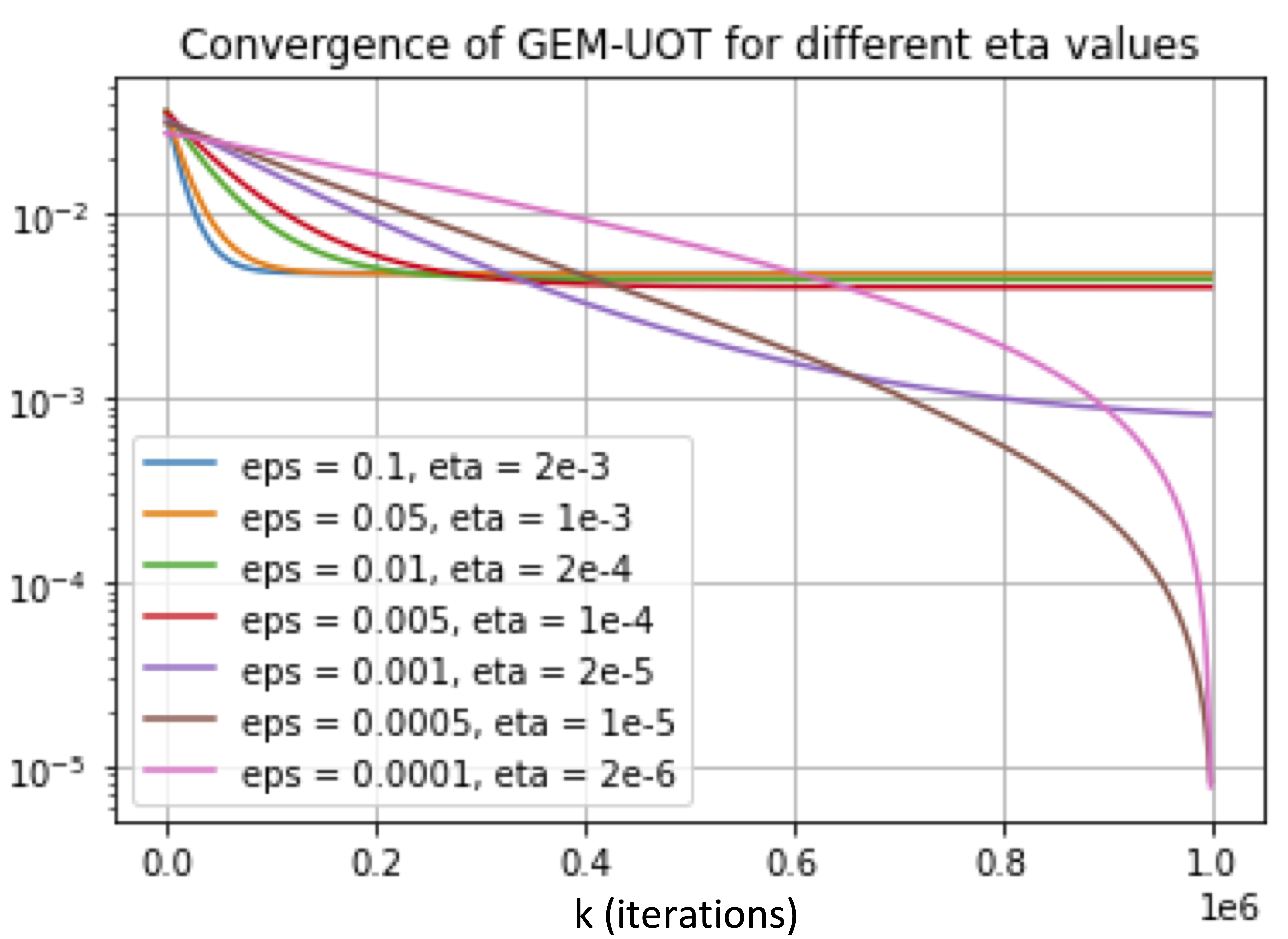
To practically validate our algorithms, we compare the GEM-UOT with Sinkhorn on CIFAR-10 dataset (Krizhevsky and Hinton, 2009). A pair of flattened images corresponds to the marginals $\mathbf{a},\mathbf{b}$, whereby the cost matrix $C$ is the matrix of $\ell_{1}$ distances between pixel locations. This is also the setting considered in (Pham et al., 2020; Dvurechensky et al., 2018). We plot the results in Figure 4, which demonstrates GEM-UOT’ superior performance. Additional experiments on Fashion-MNIST dataset that further cover GEM-RUOT are presented in Appendix D. We highlight that GEM-UOT only has logarithmic dependence on $\tau$, improving over Sinkhorn’s linear dependence on $\tau$ which had been its major bottleneck in the regime of large $\tau$ (Sejourne et al., 2022). Experiment on the scalability of $\tau$ in Figure 2, which is averaged over 10 randomly chosen image pairs, empirically reasserts our favorable dependence on $\tau$ on the CIFAR-10 dataset. In addition, we evaluate the behaviour of GEM-UOT for different levels of $\varepsilon$ and thus $\eta$ in Figure 5.
Figure 4: Primal gap $f-f^{*}$ of GEM-UOT and Sinkhorn on CIFAR-10. Figure 5: Algorithmic dependence on $\eta$ and the corresponding accuracy achieved by the algorithm on CIFAR-10 for $10^{6}$ iterations.

.

5.3 Sparsity of GEM-UOT

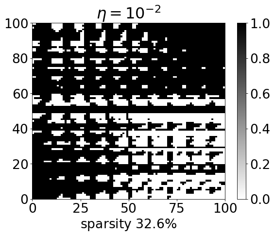
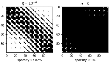
On two real datasets Fashion-MNIST and CIFAR 10, we empirically illustrate the sparseness of the transportation plans produced by GEM-UOT in Figure 6 and Figure 7, while Sinkhorn produces transportation plan with $0\%$ sparsity in those experiments. This result is consistent with (Blondel et al., 2018), where entropic regularization enforces strictly positive and dense transportation plan and squared-$\ell_{2}$ induces sparse transportation plan. To illustrate the effectiveness of $\ell_{2}$ as the sparse regularization, in Figure 8 we compare the heat maps of the optimal transportation plans of squared-$\ell_{2}$ UOT and original UOT on CIFAR 10. We set the sparsity threshold of $10^{-2}$ and report the sparsity results in the following figures.
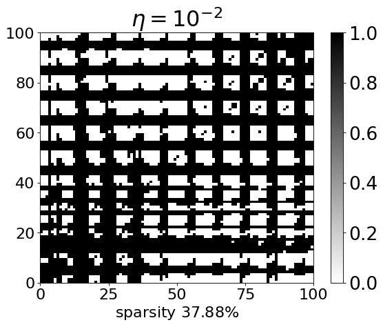
Figure 6: $37.88\%$ sparsity on Fashion-MNIST. Figure 7: $32.6\%$ sparsity on CIFAR-10. Figure 8: Sparsity of squared-$\ell_{2}$ UOT plan (left) versus original UOT plan (right) on CIFAR 10.

5.4 Color Transfer

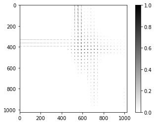
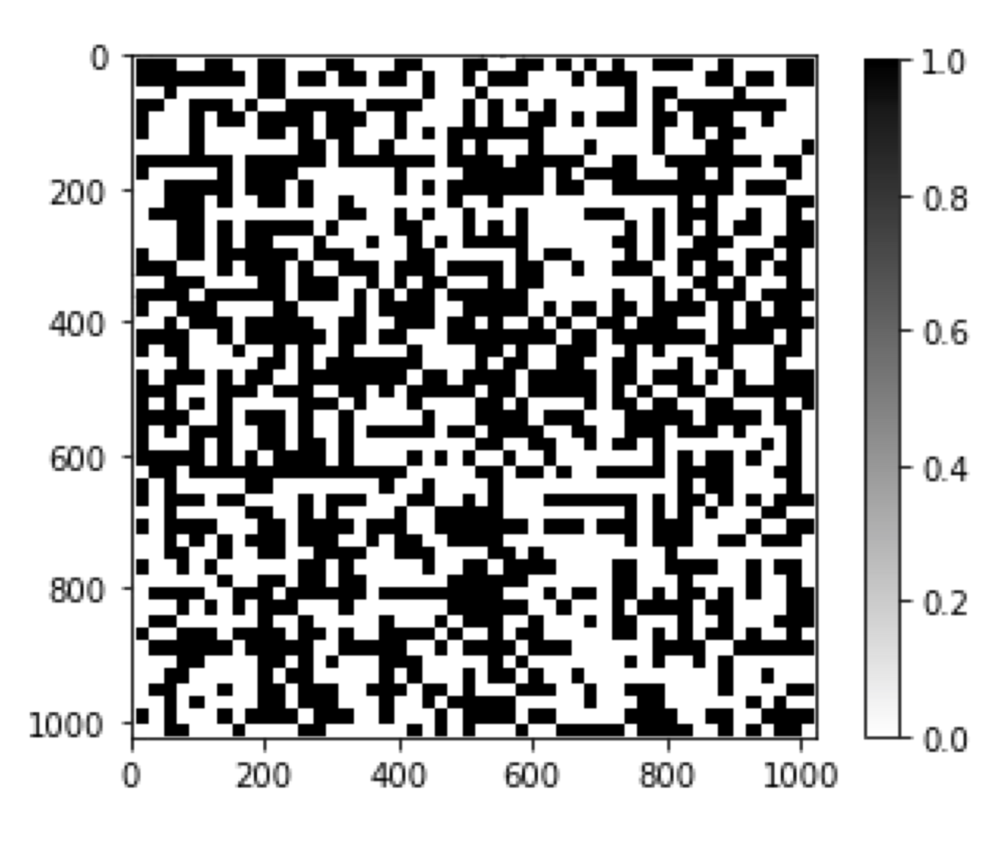
Color transfer is a prominent application where sparse transportation plan is of special interest (Blondel et al., 2018). This experiment shows that squared-$\ell_{2}$ UOT (i.e. sparse UOT) solved by GEM-UOT results in a sparse transportation plan and is thus congruent with this application, while entropic UOT solved by Sinkhorn results in strictly positive and dense transportation plan, hindering its adoption. In particular, we conduct the UOT between the histograms of two images. Given the source image $X$ and target image $Y$ both of size $l\times h$, we present their pixels in RGB space. Quantizing the images down to $n$ colors, we obtain the color centroids for the source and target images respectively as $S_{source}=\{x_{1},x_{2},...,x_{n}\}$ and $S_{target}=\{y_{1},y_{2},...,y_{n}\}$, where $x_{i},y_{i}\in\mathbb{R}^{3}$. Then the source image’s color histogram $\mathbf{a}\in\Delta^{n}$ is computed as the empirical distribution of pixels over the $n$ centroids, i.e. $a_{k}=\frac{1}{lh}\cdot\big{(}\sum_{i=1}^{l}\sum_{j=1}^{h}\mathbbm{1}\{X_{ij}\in x_{k}\}\big{)}$. The target image’s color histogram $\mathbf{b}\in\Delta^{n}$ is computed similarly. We compute the transportation plan between the two images via sparse UOT solved by GEM-UOT and entropic UOT solved by Sinkhorn, and report their qualities of color transfer in Figure 9, and the sparsity in Figure 10 and Figure 11. To demonstrate how entropic regularized UOT tend to generate dense mappings, we set the sparsity threshold of $10^{-2}$ for Figure 11 while the sparsity threshold for Figure 10 is $0$. (Note that due to the entropic regularization, Sinkhorn has $0\%$ sparsity under such threshold.)
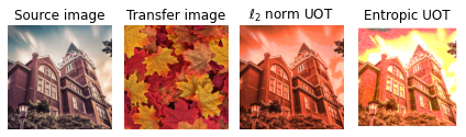
Figure 9: Quality of color transfer by GEM-UOT (solving squared-$\ell_{2}$ UOT) and Sinkhorn (solving entropic UOT). Figure 10: GEM-UOT gets $99.4\%$ sparsity. Figure 11: Sinkhorn gets $51\%$ sparsity.

5.5 Approximation Error between UOT and OT

5.5.1 Approximation of OT Transportation Plan and OT Retrieval Gap

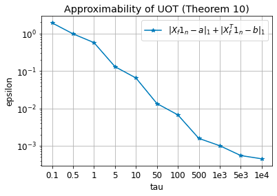
Figure 12: Approximability of OT via UOT (Theorem 23) on synthetic data. The gap approaches $0$ with rate $O\left(\frac{n}{\tau}\right)$, as $\tau$ grows.

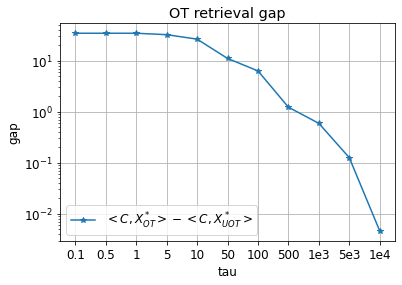
Figure 13: OT retrieval of GEM-OT (Theorem 24) on CIFAR-10. This empirically verifies vanishing OT retrieval gap for $\tau\to\infty$.

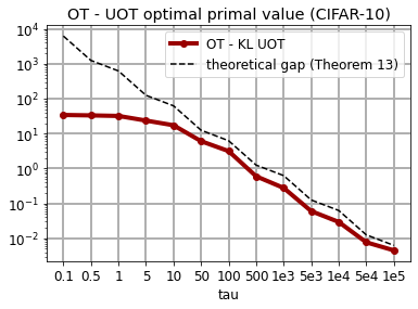
Figure 14: The error $\mathbf{OT}(\mathbf{a},\mathbf{b})-\mathbf{UOT}_{\mathbf{KL}}(\mathbf{a},\mathbf{b})$ (Theorem 26) in terms of the empirical gap (red) and the theoretical gap (black dotted) on the CIFAR-10.

We investigate the approximability of OT via UOT in terms of transportation plan (Theorem 23) on synthetic data where $\alpha=\beta=1$ and entries of $C$ are drawn uniformly from $[0.5,1]$. The result is depicted in Figure 12. Next, we verify the error incurred by GEM-OT (Algorithm 3) for retrieving OT solution from UOT. The choice of $\tau$ in GEM-OT equivalently means that the retrieval gap $\varepsilon$ established in Theorem 24 can be upperbounded by $\frac{16\|C\|_{\infty}n\gamma}{\tau}$ where $\gamma=\|C\|_{\infty}+\varepsilon/32$. To assert such vanishing effect of the error as $\tau$ grows large, we test on CIFAR-10 dataset and report the OT retrieval gap in Figure 13. We note that the OT retrieval gap also upperbounds the approximation error in transportation plan, so Figure 13 also serves as empirical verification of Theorem 23 on CIFAR-10 data.

5.5.2 Approximation Error between UOT and OT Distances

On CIFAR-10 data, we measure the gap $\mathbf{OT}(\mathbf{a},\mathbf{b})-\mathbf{UOT}_{\mathbf{KL}}(\mathbf{a},\mathbf{b})$ of transport distance between OT and UOT (Theorem 26) in Figure 14. The result illustrates the sharpness of our theoretical bound and the trade-off between $\tau$ and approximation error, which can further elucidate more refined tuning of $\tau$.

6 Conclusion

We have developed a new algorithm for solving the discrete UOT problem using gradient-based methods. Our method achieves the complexity of $\widetilde{O}\big{(}\kappa n^{2}\big{)}\big{)}$, where $\kappa$ is the condition number depending on only the two input measures. This is significantly better than the only known complexity ${O}\big{(}\frac{\tau n^{2}\log(n)}{\varepsilon}\log\big{(}\frac{\log(n)}{{\varepsilon}}\big{)}\big{)}$ of Sinkhorn algorithm (Pham et al., 2020) to the UOT problem in terms of $\varepsilon$ and $\tau$ dependency. In addition, we are the first to theoretically analyze the approximability of the UOT problem to find an OT solution. Our numerical results show the efficiency of the new method and the tightness of our theoretical bounds. We believe that our analysis framework can be extended to study the convergence results of stochastic methods, widely used in ML applications for handling large-scale datasets (Nguyen et al., 2018) or under nonlinear stochastic control settings (Nguyen and Maguluri, 2023). Our results on approximation error can open up directions that utilize UOT to approximate standard OT and even partial OT (Nguyen et al., 2024) using first-order methods.

APPENDIX

Appendix A Sinkhorn Algorithm

A.1 Regularity Conditions

In this Section, we will show that the assumptions used by the Sinkhorn (Pham et al., 2020) algorithm are equivalent to our stated regularity conditions (S1)-(S4). (S4) is clearly stated in their list of regularity conditions. To claim their complexity, in (Pham et al., 2020, Corollary1), they further require the condition ’$R=O(\frac{1}{\eta}\|C\|_{\infty})$’. Following their discussion in (Pham et al., 2020, Section 3.1), a necessary condition for it to hold is $\left\lVert\log(\mathbf{a})\right\rVert_{\infty}=O(\log(n))$ (and resp. $\left\lVert\log(\mathbf{b})\right\rVert_{\infty}=O(\log(n))$). To see that $\left\lVert\log(\mathbf{a})\right\rVert_{\infty}=O(\log(n))$ (and resp. $\left\lVert\log(\mathbf{b})\right\rVert_{\infty}=O(\log(n))$) is equivalent to (S1)-(S3), we note that if $a_{min}=0$ then $\left\lVert\log(\mathbf{a})\right\rVert_{\infty}=\infty$ (contradiction!), and $\left\lVert\log(\mathbf{a})\right\rVert_{\infty}=\max\{|\log(a_{min})|,|\log(a_{max})|\}$.

A.2 The dependency of Sinkhorn complexity on $\log(\alpha+\beta)$

We note that in its pure form, Sinkhorn’s complexity has $\log(\alpha+\beta)$, which is excluded in (Pham et al., 2020) under their regularity condition (S4) that $\alpha,\beta$ are constants. To see this, note that in the proof of (Pham et al., 2020, Corollary1), their quantity $U$ has the complexity $O((\alpha+\beta)\log(n))$ and appears in Sinkhorn’s final complexity as $\log(U)$.

Appendix B Supplementary Lemmas and Theorems

Lemma 28

For $x,y\in\mathbb{R}$, we have: $|\max\{0,x\}-\max\{0,y\}|\leq|x-y|$

Proof  We have:

$$\max\{0,x\}=\max\{0,x-y+y\} \leq\max\{0,y\}+\max\{0,x-y\}\leq\max\{0,y\}+|x-y|$$

$$\max\{0,x\}-\max\{0,y\} \leq|x-y|$$

By symmetry, $\max\{0,y\}-\max\{0,x\}\leq|x-y|$. Thus, $|\max\{0,x\}-\max\{0,y\}|\leq|x-y|$.  

Theorem 29 (Rockafellar (1967))

Let $(E,E^{*})$ and $(F,F^{*})$ be two couples of topologically paired spaces. Let $A:E\rightarrow F$ be a continuous linear operator and $A^{*}:F^{*}\rightarrow E^{*}$ its adjoint. Let f and g be lower semicontinuous and proper convex functions defined on E and F respectively. If there exists $x\in domf$ such that g is continuous at $Ax$, then

$$\sup_{x\in E}-f(-x)-g(Ax)=\inf_{y^{*}\in F^{*}}f^{*}(A^{*}y^{*})+g^{*}(y^{*})$$

Moreover, if there exists a maximizer $x\in E$ then there exists $y^{*}\in F^{*}$ satisfying $Ax\in\partial g^{*}(y^{*})$ and $A^{*}y^{*}\in\partial f(-x)$.

Lemma 30 (Lemma 7, (Altschuler et al., 2017))

For the inputs $X\in\mathbb{R}^{n\times n},\mathbf{a}\in\mathbb{R}^{n}$ and $\mathbf{b}\in\mathbb{R}^{n}$, Algorithm 4 takes $O(n^{2})$ time to output a matrix $Y\in\Pi(\mathbf{a},\mathbf{b})$ satisfying:

$$\|Y-X\|_{1}\leq 2[\|X\textbf{1}_{n}-\mathbf{a}\|_{1}+\|X^{\top}\textbf{1}_{n}-\mathbf{b}\|_{1}]$$ (78)

Appendix C Missing Proofs

C.1 Proof of Lemma 14

Let $\mathbf{x}^{*}=(\mathbf{u}^{*},\mathbf{v}^{*},\mathbf{t}^{*})$ be an optimal solution to (11). Because of the projection step on line 8 of Algorithm 1, we have $\underline{\mathbf{x}}^{t},\mathbf{x}^{t}\in V_{D}$ for $t=0,\dots,k$. By Lemma 11, $f_{\eta}(\mathbf{x})$ is $L$-smooth and $w_{\eta}(\mathbf{x})$ is $\mu$-strongly convex on $conv\{\mathbf{x}^{*},\underline{\mathbf{x}}^{0},\mathbf{x}^{0},\underline{\mathbf{x}}^{1},\mathbf{x}^{1},...\}$ The GEM-UOT is based on the GEM being applied to solve the dual objective (38), which, from (Lan and Zhou, 2018, Theorem 2.1) and the proof therein, thus guarantees that the dual iterate $\underline{\mathbf{x}}^{k}$ converges to the dual solution $\mathbf{x}^{*}$ of (38) by:

$$\|\underline{\mathbf{x}}^{k}-\mathbf{x}^{*}\|_{2}^{2} \leq\frac{4\Delta_{0,\sigma_{0}}k\zeta^{k}(1-\zeta)}{\mu(1-\zeta^{k})}.$$ (79)

Furthermore, we have:

$$\frac{k\zeta^{k}(1-\zeta)}{1-\zeta^{k}} =\big{(}\sum_{t=1}^{k}\frac{\zeta^{t}}{\zeta^{t}}\big{)}\frac{\zeta^{k}(1-\zeta)}{1-\zeta^{k}}\leq\big{(}\sum_{t=1}^{k}\frac{\zeta^{t}}{\zeta^{1.5t}}\big{)}\frac{\zeta^{k}(1-\zeta)}{1-\zeta^{k}}$$

$$\leq\frac{1-\zeta^{k/2}}{\zeta^{k/2}(1-\zeta^{1/2})}\frac{\zeta^{k}(1-\zeta)}{1-\zeta^{k}}$$

$$\leq 2\zeta^{k/2}$$ (80)

Now, plugging (80) into (79) gives:

$$\|\underline{\mathbf{x}}^{k}-\mathbf{x}^{*}\|_{2}^{2} \leq\frac{8\Delta_{0,\sigma_{0}}\zeta^{k/2}}{\mu}$$ (81)

Line 16 of Algorithm 1 further converts the dual iterate $\underline{\mathbf{x}}^{k}$ into the primal iterate $X^{k}$ as the final output. Next, we show that the convergence of the dual iterate in the sense of (81) leads to the convergence of the primal iterate $X^{k}$ to the primal solution $X^{\eta}$ of the primal objective (5). From the definition of $X^{k}$ in Algorithm 1 and in view of Corollary 5, we have:

$$\|X^{k}-X^{\eta}\|_{1} =\frac{1}{2\eta}\sum_{i,j=1}^{n}|\underline{t}^{k}_{ij}-t^{*}_{ij}|$$

$$\leq\frac{1}{2\eta}\|\underline{\mathbf{x}}^{k}-\mathbf{x}^{*}\|_{1}\leq\frac{\sqrt{n^{2}+2n}}{2\eta}\|\underline{\mathbf{x}}^{k}-\mathbf{x}^{*}\|_{2}$$

$$\overset{\eqref{baby1}}{\leq}\frac{\sqrt{2}n}{2\eta\mu}2\sqrt{2}\Delta_{0,\sigma_{0}}^{1/2}\zeta^{k/4}=\frac{2n\Delta_{0,\sigma_{0}}^{1/2}}{\eta\mu}(1-\frac{1}{1+\sqrt{1+16L/\mu}})^{k/4}$$

$$\leq\frac{2n\Delta_{0,\sigma_{0}}^{1/2}}{\eta\mu}\cdot exp\{-\frac{k}{4(1+\sqrt{1+16L/\mu})}\}.$$

The condition that $\frac{2n\Delta_{0,\sigma_{0}}^{1/2}}{\eta\mu}\cdot exp\{-\frac{k}{4(1+\sqrt{1+16L/\mu})}\}\leq\min\{\frac{\varepsilon}{2L_{1}},\frac{\min\{a_{min},b_{min}\}e^{-D/\tau}}{2},\frac{\alpha+\beta}{2}\}$ is equivalent to:

$$k\geq 4(1+\sqrt{1+16L/\mu})\log\bigg{(}\frac{4n\Delta_{0,\sigma_{0}}^{1/2}}{\eta\mu}\max\bigg{\{}\frac{L_{1}}{\varepsilon},\frac{e^{D/\tau}}{\min\{a_{min},b_{min}\}},(\alpha+\beta)^{-1}\bigg{\}}\bigg{)}=K_{0}.$$

Therefore,

$$\|X^{k}-X^{\eta}\|_{1}\leq\min\bigg{\{}\frac{\varepsilon}{2L_{1}},\frac{\min\{a_{min},b_{min}\}e^{-D/\tau}}{2},\frac{\alpha+\beta}{2}\bigg{\}}.$$ (82)

C.2 Proof of Lemma 15

For $p=\frac{1}{2}\min\{a_{min},b_{min}\}e^{-\frac{D}{\tau}}$ and $q=\alpha+\beta$ given in Section 3.1, we know that $X^{\eta}\in U_{p,q}$ by Lemma 9. We now proceed to prove that $X^{k}\in U_{p,q}$. Consider any $i\in[1,n]$:

$$\sum_{j=1}^{n}X^{k}_{ij} \geq\sum_{j=1}^{n}X^{\eta}_{ij}-|\sum_{j=1}^{n}(X^{k}_{ij}-X^{\eta}_{ij})|\geq\sum_{j=1}^{n}X^{\eta}_{ij}-\|X^{k}-X^{\eta}\|_{1}\overset{\eqref{gradient_cond1}}{=}a_{i}e^{-u_{i}/\tau}-\|X^{k}-X^{\eta}\|_{1}$$

$$\overset{\eqref{opt_sol_bounds3}}{\geq}a_{min}e^{-D/\tau}-\|X^{k}-X^{\eta}\|_{1}\overset{\eqref{misc_bound1}}{\geq}\frac{a_{min}e^{-D/\tau}}{2}\geq p,$$

$$\sum_{j=1}^{n}X^{k}_{ij} \leq\sum_{j=1}^{n}X^{\eta}_{ij}+|\sum_{j=1}^{n}(X^{k}_{ij}-X^{\eta}_{ij})|\leq\|X^{\eta}\|_{1}+\|X^{k}-X^{\eta}\|_{1}\overset{\eqref{opt_sol_bounds1},\eqref{misc_bound1}}{\leq}\frac{\alpha+\beta}{2}+\frac{\alpha+\beta}{2}=\alpha+\beta.$$

Similarly, for any $j\in[1,n]$, we have: $p\leq\sum_{i=1}^{n}X^{k}_{ij}\leq q$, and thus conclude that $X^{k}\in U_{p,q}$.

C.3 Proof of Lemma 11

The gradient of $f_{\eta}(\mathbf{x}=(\mathbf{u},\mathbf{v},\mathbf{t}))$ can be computed as:

$$\frac{\partial f_{\eta}}{\partial u_{i}}=-a_{i}e^{-u_{i}/\tau}-\frac{\min\{a_{min},b_{min}\}}{\tau}e^{-D/\tau}u_{i},$$

$$\frac{\partial f_{\eta}}{\partial v_{j}}=-b_{j}e^{-v_{j}/\tau}-\frac{\min\{a_{min},b_{min}\}}{\tau}e^{-D/\tau}v_{j},$$

$$\frac{\partial f_{\eta}}{\partial t_{ij}}=0.$$

The Hessian of $f_{\eta}(\mathbf{x}=(\mathbf{u},\mathbf{v},\mathbf{t}))$ can be computed as:

$$\frac{\partial^{2}f_{\eta}}{\partial u_{i}\partial v_{j}}=\frac{\partial^{2}f_{\eta}}{\partial u_{i}\partial t_{kj}}=\frac{\partial^{2}f_{\eta}}{\partial v_{i}\partial t_{kj}}=0,$$

$$\frac{\partial^{2}f_{\eta}}{\partial u_{i}^{2}}=\frac{a_{i}}{\tau}e^{-u_{i}/\tau}-\frac{\min\{a_{min},b_{min}\}}{\tau}e^{-D/\tau},$$

$$\frac{\partial^{2}f_{\eta}}{\partial v_{j}^{2}}=\frac{b_{j}}{\tau}e^{-v_{j}/\tau}-\frac{\min\{a_{min},b_{min}\}}{\tau}e^{-D/\tau}.$$

If $\mathbf{x}\in V_{D}$, then $u_{i},v_{j}\leq D$ for all $i,j\in[n]$ which implies $\frac{\partial^{2}f_{\eta}}{\partial u_{i}^{2}},\frac{\partial^{2}f_{\eta}}{\partial v_{j}^{2}}\geq 0$ for all $i,j\in[n]$ and thereby $\nabla^{2}f_{\eta}(\mathbf{x})\succcurlyeq 0$ on $V_{D}$. We can then conclude that $f_{\eta}(\mathbf{x})$ is convex on $V_{D}$.

Now let us consider any $\mathbf{x}=(\mathbf{u},\mathbf{v},\mathbf{t}),\mathbf{x}^{\prime}=(\mathbf{u}^{\prime},\mathbf{v}^{\prime},\mathbf{t}^{\prime})\in V_{D}$. By Mean Value Theorem, $\exists c_{i}\in range(u_{i},u_{i}^{\prime})$, such that $e^{-u_{i}/\tau}-e^{-u_{i}^{\prime}/\tau}=-\frac{1}{\tau}e^{-c_{i}/\tau}(u_{i}-u_{i}^{\prime})$ and $\exists d_{j}\in range(v_{j},v_{j}^{\prime})$, such that $e^{-v_{j}/\tau}-e^{-v_{j}^{\prime}/\tau}=-\frac{1}{\tau}e^{-d_{i}/\tau}(v_{j}-v_{j}^{\prime})$. We then obtain:

$$\|\nabla f_{\eta}(\mathbf{x})-\nabla f_{\eta}(\mathbf{x}^{\prime})\|_{2}^{2}= \sum_{i=1}^{n}\bigg{[}\big{(}\frac{a_{i}}{\tau}e^{-c_{i}/\tau}-\frac{\min\{a_{min},b_{min}\}}{\tau}e^{-D/\tau}\big{)}(u_{i}-u^{\prime}_{i})\bigg{]}^{2}$$

$$+\sum_{j=1}^{n}\bigg{[}\big{(}\frac{b_{j}}{\tau}e^{-d_{j}/\tau}-\frac{\min\{a_{min},b_{min}\}}{\tau}e^{-D/\tau}\big{)}(v_{j}-v^{\prime}_{j})\bigg{]}^{2}$$

$$\leq \sum_{i=1}^{n}\big{(}\frac{a_{i}}{\tau}e^{-c_{i}/\tau}+\frac{\min\{a_{min},b_{min}\}}{\tau}e^{-D/\tau}\big{)}^{2}(u_{i}-u^{\prime}_{i})^{2}$$

$$+\sum_{j=1}^{n}\big{(}\frac{b_{j}}{\tau}e^{-d_{j}/\tau}+\frac{\min\{a_{min},b_{min}\}}{\tau}e^{-D/\tau}\big{)}^{2}(v_{j}-v^{\prime}_{j})^{2}$$

$$\leq \sum_{i=1}^{n}\big{(}\frac{a_{i}}{\tau}\frac{\alpha+\beta}{2a_{i}}+\frac{\min\{a_{min},b_{min}\}}{\tau}e^{-D/\tau}\big{)}^{2}(u_{i}-u^{\prime}_{i})^{2}$$

$$+\sum_{j=1}^{n}\big{(}\frac{b_{j}}{\tau}\frac{\alpha+\beta}{2b_{j}}+\frac{\min\{a_{min},b_{min}\}}{\tau}e^{-D/\tau}\big{)}^{2}(v_{j}-v^{\prime}_{j})^{2}$$

(since $$c_{i}\in range(u_{i},u_{i}^{\prime}) c_{i}\geq\tau\log(\frac{2a_{i}}{\alpha+\beta}) d_{j}\geq\tau\log(\frac{2b_{j}}{\alpha+\beta})$$, . Similarly, )

$$\leq \bigg{(}\frac{\alpha+\beta}{2\tau}+\frac{\min\{a_{min},b_{min}\}}{\tau}e^{-D/\tau}\bigg{)}^{2}\|\mathbf{x}-\mathbf{x}^{\prime}\|_{2}^{2}.$$

$$\|\nabla f_{\eta}(\mathbf{x})-\nabla f_{\eta}(\mathbf{x}^{\prime})\|_{2}\leq \bigg{(}\frac{\alpha+\beta}{2\tau}+\frac{\min\{a_{min},b_{min}\}}{\tau}e^{-D/\tau}\bigg{)}\|\mathbf{x}-\mathbf{x}^{\prime}\|_{2},$$

which implies that $f_{\eta}(\mathbf{x})$ is $L$-smooth with $L=\frac{\alpha+\beta}{2\tau}+\frac{\min\{a_{min},b_{min}\}}{\tau}e^{-D/\tau}$.

Now let us consider $w_{\eta}(\mathbf{x})$. The gradient $w_{\eta}(\mathbf{x})$ can be computed as:

$$\frac{\partial w}{\partial u_{i}}=\frac{\min\{a_{min},b_{min}\}}{\tau}e^{-D/\tau}u_{i},\quad\frac{\partial w}{\partial v_{j}}=\frac{\min\{a_{min},b_{min}\}}{\tau}e^{-D/\tau}v_{j},\quad\frac{\partial w}{\partial t_{ij}} =\frac{1}{2\eta}t_{ij}.$$

For any $\mathbf{x}=(\mathbf{u},\mathbf{v},\mathbf{t}),\mathbf{x}^{\prime}=(\mathbf{u}^{\prime},\mathbf{v}^{\prime},\mathbf{t}^{\prime})\in V_{D}$, we have:

$$\left\langle\nabla w_{\eta}(\mathbf{x})-\nabla w_{\eta}(\mathbf{x}^{\prime}),\mathbf{x}-\mathbf{x}^{\prime}\right\rangle =\sum_{i=1}^{n}\frac{\min\{a_{min},b_{min}\}}{\tau}e^{-D/\tau}(u_{i}-u_{i}^{\prime})^{2}$$

$$+\sum_{j=1}^{n}\frac{\min\{a_{min},b_{min}\}}{\tau}e^{-D/\tau}(v_{j}-v_{j}^{\prime})^{2}+\sum_{i,j=1}^{n}\frac{1}{2\eta}(t_{ij}-t^{\prime}_{ij})^{2}$$

$$\geq\min\bigg{\{}\frac{\min\{a_{min},b_{min}\}}{\tau}e^{-D/\tau},\frac{1}{2\eta}\bigg{\}}\|\mathbf{x}-\mathbf{x}^{\prime}\|_{2}^{2}.$$

Therefore, $w_{\eta}(\mathbf{x})$ is $\mu$-strongly convex on $V_{D}$ with $\mu=\min\bigg{\{}\frac{\min\{a_{min},b_{min}\}}{\tau}e^{-D/\tau},\frac{1}{2\eta}\bigg{\}}$.

C.4 Projection Step of GEM-UOT

We describe the following projection step (i.e. line 8 in Algorithm 1) in more details:

$$\mathbf{x}^{t} =\mathcal{M}_{V_{D}\cap\mathcal{X}}(\widetilde{\mathbf{y}}^{t},\mathbf{x}^{t-1},\rho)=\mathop{\mathrm{argmin}}_{\mathbf{x}=(\mathbf{u},\mathbf{v},\mathbf{t})\in V_{D}\cap\mathcal{X}}\{G(\mathbf{x}):=\langle\widetilde{\mathbf{y}}^{t},\mathbf{x}\rangle+w_{\eta}(\mathbf{x})+\rho P(\mathbf{x}^{t-1},\mathbf{x})\}$$ (83)

where we further expand the objective $G(\mathbf{x})$ as:

$$G(\mathbf{x}) =\langle\widetilde{\mathbf{y}}^{t},\mathbf{x}\rangle+w_{\eta}(\mathbf{x})+\frac{\rho}{\mu}[w_{\eta}(\mathbf{x})-w_{\eta}(\mathbf{x}^{t-1})-\langle\nabla w_{\eta}(\mathbf{x}^{t-1}),\mathbf{x}-\mathbf{x}^{t-1}\rangle]$$

$$=\big{(}1+\frac{\rho}{\mu}\big{)}w_{\eta}(\mathbf{x})+\langle\widetilde{\mathbf{y}}^{t}-\frac{\rho}{\mu}\nabla w_{\eta}(\mathbf{x}^{t-1}),\mathbf{x}\rangle+\frac{\rho}{\mu}\langle\nabla w_{\eta}(\mathbf{x}^{t-1}),\mathbf{x}^{t-1}\rangle.$$ (84)

For abbreviation, we let $\widetilde{\mathbf{y}}^{t}-\frac{\rho}{\mu}\nabla w_{\eta}(\mathbf{x}^{t-1})=(\mathbf{u}^{c},\mathbf{v}^{c},\mathbf{t}^{c})\in\mathbb{R}^{n^{2}+2n}$ where $\mathbf{u}^{c}\in\mathbb{R}^{n},\mathbf{v}^{c}\in\mathbb{R}^{n}$ and $\mathbf{t}^{c}\in\mathbb{R}^{n^{2}}$ respectively are coefficients of the variables $\mathbf{u},\mathbf{v},\mathbf{t}$ in the linear term of (84). We also define the constants $q_{1}=\big{(}1+\frac{\rho}{\mu}\big{)}\cdot\frac{\min\{a_{min},b_{min}\}}{2\tau}e^{-D/\tau}$ and $q_{2}=\big{(}1+\frac{\rho}{\mu}\big{)}/(4\eta)$. The objective $G(\mathbf{x})$ can be written as the sum of quadratic functions as follows:

$$G(\mathbf{x})=(q_{1}\|\mathbf{u}\|_{2}^{2}+\langle\mathbf{u}^{c},\mathbf{u}\rangle)+(q_{1}\|\mathbf{v}\|_{2}^{2}+\langle\mathbf{v}^{c},\mathbf{v}\rangle)+(q_{2}\|\mathbf{t}\|_{2}^{2}+\langle\mathbf{t}^{c},\mathbf{t}\rangle)+\frac{\rho}{\mu}\langle\nabla w_{\eta}(\mathbf{x}^{t-1}),\mathbf{x}^{t-1}\rangle.$$ (85)

And the projection step is thus equivalent to solving:

$$\min_{\mathbf{x}=(\mathbf{u},\mathbf{v},\mathbf{t})\in V_{D}\cap\mathcal{X}} G(\mathbf{x})$$ (86)

$$\text{where }V_{D}\cap\mathcal{X}=\{(\mathbf{u},\mathbf{v},\mathbf{t})| \mathbf{u},\mathbf{v}\in\mathbb{R}^{n},\mathbf{t}\in\mathbb{R}^{n\times n}:\forall i,j\in[1,n],$$

$$\tau\log(\frac{2a_{i}}{\alpha+\beta})\leq u_{i}\leq D$$

$$\tau\log(\frac{2b_{j}}{\alpha+\beta})\leq v_{j}\leq D$$

$$0\leq t_{ij},$$

$$u_{i}+v_{j}-C_{ij}\leq t_{ij}\}.$$

Next, we aim to derive a simplified equivalence form of (86) that is obtained by expressing the optimal $\mathbf{t}$ with respect to fixed $\mathbf{u},\mathbf{v}$, and consequently optimizing over $\mathbf{u},\mathbf{v}$. In particular, we consider the mapping $\mathbf{t}(\mathbf{u},\mathbf{v}):\mathbb{R}^{2n}\to\mathbb{R}^{n^{2}}$ defined by:

$$t_{ij}(\mathbf{u},\mathbf{v})=\max\big{\{}0,-\frac{t_{ij}^{c}}{q_{2}},u_{i}+v_{j}-C_{ij}\big{\}},\quad\forall i,j\in[n],$$ (87)

the restricted domain $\widetilde{V}_{D}$ as follows:

$$\widetilde{V}_{D}=\{(\mathbf{u},\mathbf{v})| \mathbf{u},\mathbf{v}\in\mathbb{R}^{n}:\forall i\in[n],$$

$$\tau\log(\frac{2a_{i}}{\alpha+\beta})\leq u_{i}\leq D$$

$$\tau\log(\frac{2b_{i}}{\alpha+\beta})\leq v_{i}\leq D\},$$ (88)

and the objective:

$$\widetilde{G}(\mathbf{u},\mathbf{v})=G(\mathbf{u},\mathbf{v},\mathbf{t}(\mathbf{u},\mathbf{v})).$$ (89)

The next Lemma establishes the equivalence form for the projection problem (86).

Lemma 31

The following holds:

$$\min_{\mathbf{x}=(\mathbf{u},\mathbf{v},\mathbf{t})\in V_{D}\cap\mathcal{X}} G(\mathbf{x})=\min_{(\mathbf{u},\mathbf{v})\in\widetilde{V}_{D}}\widetilde{G}(\mathbf{u},\mathbf{v})$$ (90)

Proof  For any $(\mathbf{u},\mathbf{v})\in\widetilde{V}_{D}$, we have $\mathbf{t}(\mathbf{u},\mathbf{v})$ that is defined as in (87) satisfies:

$$0\leq t_{ij}(\mathbf{u},\mathbf{v}),$$

$$u_{i}+v_{j}-C_{ij}\leq t_{ij}(\mathbf{u},\mathbf{v}),$$

Thus, we have $(\mathbf{u},\mathbf{v},\mathbf{t}(\mathbf{u},\mathbf{v}))\in V_{D}$, which implies:

$$\min_{\mathbf{x}=(\mathbf{u},\mathbf{v},\mathbf{t})\in V_{D}\cap\mathcal{X}}G(\mathbf{x})\leq G(\mathbf{u},\mathbf{v},\mathbf{t}(\mathbf{u},\mathbf{v}))=\widetilde{G}(\mathbf{u},\mathbf{v}),\quad\forall(\mathbf{u},\mathbf{v})\in\widetilde{V}_{D}$$

$$\therefore \min_{\mathbf{x}=(\mathbf{u},\mathbf{v},\mathbf{t})\in V_{D}\cap\mathcal{X}}G(\mathbf{x})\leq\min_{(\mathbf{u},\mathbf{v})\in\widetilde{V}_{D}}\widetilde{G}(\mathbf{u},\mathbf{v}).$$ (91)

Now, take any $\mathbf{x}=(\mathbf{u},\mathbf{v},\mathbf{t})\in V_{D}\cap\mathcal{X}$. We fix $\mathbf{u}$ and $\mathbf{v}$, and optimize over all $\mathbf{t}^{\prime}$ such that $(\mathbf{u},\mathbf{v},\mathbf{t}^{\prime})\in V_{D}\cap\mathcal{X}$, i.e. those $\mathbf{t}^{\prime}$ with $0\leq t^{\prime}_{ij}$ and $u_{i}+v_{j}-C_{ij}\leq t^{\prime}_{ij}$. Then, we have:

$$G(\mathbf{x}=(\mathbf{u},\mathbf{v},\mathbf{t}))\geq\min_{\mathbf{t}^{\prime}:(\mathbf{u},\mathbf{v},\mathbf{t}^{\prime})\in V_{D}\cap\mathcal{X}}G(\mathbf{u},\mathbf{v},\mathbf{t}^{\prime}).$$ (92)

Note that the optimization problem over $\mathbf{t}^{\prime}$ in the RHS of (92) has separable quadratic objective and separable linear constraints. Thus, simple algebra gives $\mathbf{t}(\mathbf{u},\mathbf{v})$ being defined in (87) as the optimal solution to such problem, i.e.

$$\mathbf{t}(\mathbf{u},\mathbf{v})=\mathop{\mathrm{argmin}}_{\mathbf{t}^{\prime}:(\mathbf{u},\mathbf{v},\mathbf{t}^{\prime})\in V_{D}\cap\mathcal{X}}G(\mathbf{u},\mathbf{v},\mathbf{t}^{\prime}).$$ (93)

From (92) and (93), we have:

$$G(\mathbf{x}=(\mathbf{u},\mathbf{v},\mathbf{t})) \geq G(\mathbf{u},\mathbf{v},\mathbf{t}(\mathbf{u},\mathbf{v}))=\widetilde{G}(\mathbf{u},\mathbf{v})$$

$$\geq\min_{(\mathbf{u},\mathbf{v})\in\widetilde{V}_{D}}\widetilde{G}(\mathbf{u},\mathbf{v})$$

$$\therefore\min_{\mathbf{x}=(\mathbf{u},\mathbf{v},\mathbf{t})\in V_{D}\cap\mathcal{X}}G(\mathbf{x}) \geq\min_{(\mathbf{u},\mathbf{v})\in\widetilde{V}_{D}}\widetilde{G}(\mathbf{u},\mathbf{v}),$$ (94)

where the second inequality is because any $\mathbf{x}=(\mathbf{u},\mathbf{v},\mathbf{t})\in V_{D}\cap\mathcal{X}$ implies $(\mathbf{u},\mathbf{v})\in\widetilde{V}_{D}$ by definition. Finally, combining (91) and (94) gives the desired statement.  

Since the equivalence form $\min_{(\mathbf{u},\mathbf{v})\in\widetilde{V}_{D}}\widetilde{G}(\mathbf{u},\mathbf{v})$ of the projection step is strongly convex smooth optimization over box constraints, we can adopt projected quasi-Newton method with superlinear convergence rate (Schmidt et al., 2011, Theorem 11.2), thereby resulting in $\widetilde{O}(1)$ iteration complexity. Furthermore, the per iteration cost is dominated by the gradient and Hessian computation of $\widetilde{G}$, which can be achieved efficiently in $O(n^{2})$ as follows. In particular, we have for $\forall i,j\in[n]$:

$$\frac{\partial\widetilde{G}}{\partial u_{i}} =2q_{1}u_{i}+u^{c}_{i}+2\sum_{j=1}^{n}\max\bigg{\{}0,\frac{t_{ij}^{c}}{q_{2}},u_{i}+v_{j}-C_{ij}+\frac{t_{ij}^{c}}{q_{2}}\bigg{\}},$$

$$\frac{\partial\widetilde{G}}{\partial v_{j}} =2q_{1}v_{j}+v^{c}_{j}+2\sum_{i=1}^{n}\max\bigg{\{}0,\frac{t_{ij}^{c}}{q_{2}},u_{i}+v_{j}-C_{ij}+\frac{t_{ij}^{c}}{q_{2}}\bigg{\}},$$

$$\frac{\partial^{2}\widetilde{G}}{\partial u_{i}\partial u_{j}} =\begin{cases}2q_{1}+2\sum_{k=1}^{n}\mathbbm{1}\big{\{}u_{i}+v_{k}-C_{ik}\geq\max\{0,-\frac{t_{ik}^{c}}{q_{2}}\}\big{\}},\quad\text{ if $i=j$}\\ 0,\quad\text{ otherwise}\end{cases},$$

$$\frac{\partial^{2}\widetilde{G}}{\partial v_{i}\partial v_{j}} =\begin{cases}2q_{1}+2\sum_{k=1}^{n}\mathbbm{1}\big{\{}u_{k}+v_{j}-C_{kj}\geq\max\{0,-\frac{t_{kj}^{c}}{q_{2}}\}\big{\}},\quad\text{ if $i=j$}\\ 0,\quad\text{ otherwise}\end{cases},$$

$$\frac{\partial^{2}\widetilde{G}}{\partial u_{i}\partial v_{j}} =2\mathbbm{1}\big{\{}u_{i}+v_{j}-C_{ij}\geq\max\{0,-\frac{t_{ij}^{c}}{q_{2}}\}\big{\}}.$$

Thus, we conclude that the projection step can be solved in $\widetilde{O}(n^{2})$ time.

C.5 Proof of Lemma 17

The gradient of $h_{a}(\mathbf{x}=(\mathbf{u},\mathbf{v}))$ can be computed as:

$$\frac{\partial h_{a}}{\partial u_{i}}=-a_{i}e^{-u_{i}/\tau}+\sum_{j=1}^{n}\frac{\max\{0,u_{i}+v_{j}-C_{ij}\}}{2\eta},$$

$$\frac{\partial h_{a}}{\partial v_{j}}=-b_{j}e^{-v_{j}/\tau}+\sum_{i=1}^{n}\frac{\max\{0,u_{i}+v_{j}-C_{ij}\}}{2\eta}.$$

Let us consider any $\mathbf{x}=(\mathbf{u},\mathbf{v}),\mathbf{x}^{\prime}=(\mathbf{u}^{\prime},\mathbf{v}^{\prime})\in V_{a}$. By Mean Value Theorem, $\exists c_{i}\in range(u_{i},u_{i}^{\prime})$, such that $e^{-u_{i}/\tau}-e^{-u_{i}^{\prime}/\tau}=-\frac{1}{\tau}e^{-c_{i}/\tau}(u_{i}-u_{i}^{\prime})$ and $\exists d_{j}\in range(v_{j},v_{j}^{\prime})$, such that $e^{-v_{j}/\tau}-e^{-v_{j}^{\prime}/\tau}=-\frac{1}{\tau}e^{-d_{i}/\tau}(v_{j}-v_{j}^{\prime})$. We then obtain:

$$\|\nabla h_{a}(\mathbf{x})-\nabla h_{a}(\mathbf{x}^{\prime})\|_{2}^{2}\leq 2\sum_{i=1}^{n}\bigg{[}\frac{a_{i}}{\tau}e^{-c_{i}/\tau}(u_{i}-u^{\prime}_{i})\bigg{]}^{2}+2\sum_{j=1}^{n}\bigg{[}\frac{b_{j}}{\tau}e^{-d_{j}/\tau}(v_{j}-v^{\prime}_{j})\bigg{]}^{2}$$

$$+\sum_{i=1}^{n}\frac{2}{4\eta^{2}}[\sum_{j=1}^{n}(u_{i}-u_{i}^{\prime}+v_{j}-v_{j}^{\prime})]^{2}+\sum_{j=1}^{n}\frac{2}{4\eta^{2}}[\sum_{i=1}^{n}(u_{i}-u_{i}^{\prime}+v_{j}-v_{j}^{\prime})]^{2}$$

(By Lemma 28 and simple algebra $$(x+y)^{2}\leq 2(x^{2}+y^{2})$$)

$$\leq \sum_{i=1}^{n}2\left(\frac{a_{i}}{\tau}e^{-c_{i}/\tau}\right)^{2}(u_{i}-u^{\prime}_{i})^{2}+\sum_{j=1}^{n}2\left(\frac{b_{j}}{\tau}e^{-d_{j}/\tau}\right)^{2}(v_{j}-v^{\prime}_{j})^{2}$$

$$+\sum_{i=1}^{n}\frac{1}{\eta^{2}}\{\sum_{j=1}^{n}[(u_{i}-u_{i}^{\prime})^{2}+(v_{j}-v_{j}^{\prime})^{2}]\}+\sum_{j=1}^{n}\frac{1}{\eta^{2}}\{\sum_{i=1}^{n}[(u_{i}-u_{i}^{\prime})^{2}+(v_{j}-v_{j}^{\prime})^{2}]\}$$

$$\leq\sum_{i=1}^{n}2\left(\frac{a_{i}}{\tau}\frac{\alpha+\beta}{2a_{i}}\right)^{2}(u_{i}-u^{\prime}_{i})^{2}+\sum_{j=1}^{n}2\big{(}\frac{b_{j}}{\tau}\frac{\alpha+\beta}{2b_{j}}\big{)}^{2}(v_{j}-v^{\prime}_{j})^{2}+\frac{2n}{\eta^{2}}\|\mathbf{x}-\mathbf{x}^{\prime}\|_{2}^{2}$$

(since $$c_{i}\in range(u_{i},u_{i}^{\prime}) c_{i}\geq\tau\log(\frac{2a_{i}}{\alpha+\beta}) d_{j}\geq\tau\log(\frac{2b_{j}}{\alpha+\beta})$$, . Similarly, )

$$=\left[\frac{1}{2}\cdot\bigg{(}\frac{\alpha+\beta}{\tau}\bigg{)}^{2}+\frac{2n}{\eta^{2}}\right]\|\mathbf{x}-\mathbf{x}^{\prime}\|_{2}^{2}.$$

$$\therefore \|\nabla h_{a}(\mathbf{x})-\nabla h_{a}(\mathbf{x}^{\prime})\|_{2}\leq\bigg{(}\frac{\alpha+\beta}{\tau}+\frac{2\sqrt{n}}{\eta}\bigg{)}\cdot\|\mathbf{x}-\mathbf{x}^{\prime}\|_{2}.$$

This implies that $h_{a}(\mathbf{x})$ is $L$-smooth with $L_{a}=\frac{\alpha+\beta}{\tau}+\frac{2\sqrt{n}}{\eta}$.

Appendix D Experimental Result for GEM-RUOT on Fashion-MNIST dataset

We test GEM-UOT (Algorithm 1), GEM-RUOT (Algorithm 2) and Sinkhorn on the Fashion-MNIST dataset using the same setting as the experiment on CIFAR dataset in Section 5.2 and report the result in Figure 15.

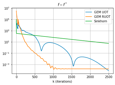
Figure 15: Comparison of $f$ primal gap between the Sinkhorn algorithm and GEM algorithms for $1500$ iterations.

References

- Agrawal et al. (2018) Akshay Agrawal, Robin Verschueren, Steven Diamond, and Stephen Boyd. A rewriting system for convex optimization problems. Journal of Control and Decision, 5(1):42–60, 2018.
- Altschuler et al. (2018) J. Altschuler, F. Bach, A. Rudi, and J. Weed. Approximating the quadratic transportation metric in near-linear time. ArXiv Preprint: 1810.10046, 2018.
- Altschuler et al. (2017) Jason Altschuler, Jonathan Weed, and Philippe Rigollet. Near-linear time approximation algorithms for optimal transport via sinkhorn iteration. In Advances in Neural Information Processing Systems, pages 1964–1974, 2017.
- Arjovsky et al. (2017) Martin Arjovsky, Soumith Chintala, and Léon Bottou. Wasserstein generative adversarial networks. In International Conference on Machine Learning, pages 214–223, 2017.
- Balaji et al. (2020) Yogesh Balaji, Rama Chellappa, and Soheil Feizi. Robust optimal transport with applications in generative modeling and domain adaptation. In H. Larochelle, M. Ranzato, R. Hadsell, M.F. Balcan, and H. Lin, editors, Advances in Neural Information Processing Systems, volume 33, pages 12934–12944. Curran Associates, Inc., 2020. URL https://proceedings.neurips.cc/paper_files/paper/2020/file/9719a00ed0c5709d80dfef33795dcef3-Paper.pdf.
- Bernton et al. (2022) Espen Bernton, Promit Ghosal, and Marcel Nutz. Entropic optimal transport: Geometry and large deviations. Duke Mathematical Journal, 171(16):3363 – 3400, 2022. doi: 10.1215/00127094-2022-0035. URL https://doi.org/10.1215/00127094-2022-0035.
- Blondel et al. (2018) M. Blondel, V. Seguy, and A. Rolet. Smooth and sparse optimal transport. In AISTATS, pages 880–889, 2018.
- Caffarelli and McCann (2010) Luis A. Caffarelli and Robert J. McCann. Free boundaries in optimal transport and monge-ampère obstacle problems. Annals of Mathematics, 171(2):673–730, 2010. ISSN 0003486X. URL http://www.jstor.org/stable/20752228.
- Chapel et al. (2021) Laetitia Chapel, Rémi Flamary, Haoran Wu, Cédric Févotte, and Gilles Gasso. Unbalanced optimal transport through non-negative penalized linear regression. In M. Ranzato, A. Beygelzimer, Y. Dauphin, P.S. Liang, and J. Wortman Vaughan, editors, Advances in Neural Information Processing Systems, volume 34, pages 23270–23282. Curran Associates, Inc., 2021. URL https://proceedings.neurips.cc/paper_files/paper/2021/file/c3c617a9b80b3ae1ebd868b0017cc349-Paper.pdf.
- Chizat et al. (2018) Lenaic Chizat, Gabriel Peyré, Bernhard Schmitzer, and François-Xavier Vialard. Scaling algorithms for unbalanced optimal transport problems. Mathematics of Computation, 87(314):2563–2609, 2018.
- Courty et al. (2017) N. Courty, R. Flamary, D. Tuia, and A. Rakotomamonjy. Optimal transport for domain adaptation. IEEE Transactions on Pattern Analysis and Machine Intelligence, 39(9):1853–1865, 2017.
- Cuturi (2013) Marco Cuturi. Sinkhorn distances: Lightspeed computation of optimal transport. In C.J. Burges, L. Bottou, M. Welling, Z. Ghahramani, and K.Q. Weinberger, editors, Advances in Neural Information Processing Systems, volume 26. Curran Associates, Inc., 2013. URL https://proceedings.neurips.cc/paper_files/paper/2013/file/af21d0c97db2e27e13572cbf59eb343d-Paper.pdf.
- De Plaen et al. (2023) Henri De Plaen, Pierre-François De Plaen, Johan A. K. Suykens, Marc Proesmans, Tinne Tuytelaars, and Luc Van Gool. Unbalanced optimal transport: A unified framework for object detection. In Proceedings of the IEEE/CVF Conference on Computer Vision and Pattern Recognition (CVPR), pages 3198–3207, June 2023.
- Dong et al. (2020) Yihe Dong, Yu Gao, Richard Peng, Ilya Razenshteyn, and Saurabh Sawlani. A study of performance of optimal transport. ArXiv Preprint: 2005.01182, 2020.
- Dvurechensky et al. (2018) P. Dvurechensky, A. Gasnikov, and A. Kroshnin. Computational optimal transport: Complexity by accelerated gradient descent is better than by Sinkhorn’s algorithm. In International conference on machine learning, pages 1367–1376, 2018.
- Essid and Solomon (2018) Montacer Essid and Justin Solomon. Quadratically regularized optimal transport on graphs. SIAM Journal on Scientific Computing, 40(4):A1961–A1986, 2018. doi: 10.1137/17M1132665. URL https://doi.org/10.1137/17M1132665.
- Fatras et al. (2021) Kilian Fatras, Thibault Sejourne, Rémi Flamary, and Nicolas Courty. Unbalanced minibatch optimal transport; applications to domain adaptation. In Marina Meila and Tong Zhang, editors, Proceedings of the 38th International Conference on Machine Learning, volume 139 of Proceedings of Machine Learning Research, pages 3186–3197. PMLR, 18–24 Jul 2021. URL https://proceedings.mlr.press/v139/fatras21a.html.
- Frogner et al. (2015) Charlie Frogner, Chiyuan Zhang, Hossein Mobahi, Mauricio Araya-Polo, and Tomaso Poggio. Learning with a wasserstein loss. In Proceedings of the 28th International Conference on Neural Information Processing Systems - Volume 2, NIPS’15, page 2053–2061, Cambridge, MA, USA, 2015. MIT Press.
- Genevay et al. (2018) Aude Genevay, Gabriel Peyre, and Marco Cuturi. Learning generative models with sinkhorn divergences. In International Conference on Artificial Intelligence and Statistics, pages 1608–1617, 2018.
- Guminov et al. (2021) Sergey Guminov, Pavel E. Dvurechensky, Nazarii Tupitsa, and Alexander V. Gasnikov. On a combination of alternating minimization and nesterov’s momentum. In International Conference on Machine Learning, 2021.
- Ho et al. (2017) Nhat Ho, XuanLong Nguyen, Mikhail Yurochkin, Hung Hai Bui, Viet Huynh, and Dinh Phung. Multilevel clustering via Wasserstein means. In Doina Precup and Yee Whye Teh, editors, Proceedings of the 34th International Conference on Machine Learning, volume 70 of Proceedings of Machine Learning Research, pages 1501–1509. PMLR, 06–11 Aug 2017. URL https://proceedings.mlr.press/v70/ho17a.html.
- Kantorovich (1942) L. V. Kantorovich. On the translocation of masses. In Dokl. Akad. Nauk. USSR (NS), volume 37, pages 199–201, 1942.
- Krizhevsky and Hinton (2009) A. Krizhevsky and G. Hinton. Learning multiple layers of features from tiny images. Master’s thesis, Department of Computer Science, University of Toronto, 2009.
- Lan and Zhou (2018) Guanghui Lan and Yi Zhou. Random gradient extrapolation for distributed and stochastic optimization. SIAM Journal on Optimization, 28(4):2753–2782, 2018.
- Le et al. (2021) Khang Le, Huy Nguyen, Quang Minh Nguyen, Tung Pham, Hung Bui, and Nhat Ho. On robust optimal transport: Computational complexity and barycenter computation. In A. Beygelzimer, Y. Dauphin, P. Liang, and J. Wortman Vaughan, editors, Advances in Neural Information Processing Systems, 2021. URL https://openreview.net/forum?id=xRLT28nnlFV.
- Lee et al. (2019) John Lee, Nicholas P Bertrand, and Christopher J Rozell. Parallel unbalanced optimal transport regularization for large scale imaging problems. ArXiv Preprint: 1909.00149, 2019.
- Lee and Sidford (2014) Yin Tat Lee and Aaron Sidford. Path finding methods for linear programming: Solving linear programs in Õ(vrank) iterations and faster algorithms for maximum flow. In 2014 IEEE 55th Annual Symposium on Foundations of Computer Science, pages 424–433, 2014. doi: 10.1109/FOCS.2014.52.
- Liero et al. (2017) Matthias Liero, Alexander Mielke, and Giuseppe Savaré. Optimal entropy-transport problems and a new hellinger–kantorovich distance between positive measures. Inventiones mathematicae, 211(3):969–1117, Dec 2017. ISSN 1432-1297. doi: 10.1007/s00222-017-0759-8. URL http://dx.doi.org/10.1007/s00222-017-0759-8.
- Lorenz et al. (2019) Dirk A. Lorenz, Paul Manns, and Christian Meyer. Quadratically regularized optimal transport. Applied Mathematics & Optimization, 83:1919 – 1949, 2019. URL https://api.semanticscholar.org/CorpusID:85517311.
- Luo et al. (2023) Yiling Luo, Yiling Xie, and Xiaoming Huo. Improved rate of first order algorithms for entropic optimal transport. In Francisco Ruiz, Jennifer Dy, and Jan-Willem van de Meent, editors, Proceedings of The 26th International Conference on Artificial Intelligence and Statistics, volume 206 of Proceedings of Machine Learning Research, pages 2723–2750. PMLR, 25–27 Apr 2023. URL https://proceedings.mlr.press/v206/luo23a.html.
- Malitsky and Mishchenko (2020) Yura Malitsky and Konstantin Mishchenko. Adaptive gradient descent without descent. In Hal Daumé III and Aarti Singh, editors, Proceedings of the 37th International Conference on Machine Learning, volume 119, pages 6702–6712, 2020.
- Muzellec et al. (2016) Boris Muzellec, Richard Nock, Giorgio Patrini, and Frank Nielsen. Tsallis regularized optimal transport and ecological inference. In AAAI Conference on Artificial Intelligence, 2016.
- Nguyen et al. (2024) Anh Duc Nguyen, Tuan Dung Nguyen, Quang Minh Nguyen, Hoang H. Nguyen, and Kim-Chuan Toh. On partial optimal transport: Revising the infeasibility of sinkhorn and efficient gradient methods. In AAAI Conference on Artificial Intelligence, 2024. URL https://arxiv.org/pdf/2312.13970.pdf.
- Nguyen and Maguluri (2023) Hoang Huy Nguyen and Siva Theja Maguluri. Stochastic approximation for nonlinear discrete stochastic control: Finite-sample bounds. ArXiv Preprint: 2304.11854, 2023.
- Nguyen et al. (2021) Khai Nguyen, Nhat Ho, Tung Pham, and Hung Bui. Distributional sliced-wasserstein and applications to generative modeling. In International Conference on Learning Representations, 2021.
- Nguyen et al. (2018) Lam Nguyen, Phuong Ha Nguyen, Marten van Dijk, Peter Richtarik, Katya Scheinberg, and Martin Takac. SGD and hogwild! Convergence without the bounded gradients assumption. In Jennifer Dy and Andreas Krause, editors, Proceedings of the 35th International Conference on Machine Learning, volume 80 of Proceedings of Machine Learning Research, pages 3750–3758. PMLR, 10–15 Jul 2018. URL https://proceedings.mlr.press/v80/nguyen18c.html.
- Peyré and Cuturi (2019) Gabriel Peyré and Marco Cuturi. Computational optimal transport. Foundations and Trends® in Machine Learning, 11(5-6):355–607, 2019.
- Pham et al. (2020) Khiem Pham, Khang Le, Nhat Ho, Tung Pham, and Hung Bui. On unbalanced optimal transport: An analysis of Sinkhorn algorithm. In Hal Daumé III and Aarti Singh, editors, Proceedings of the 37th International Conference on Machine Learning, volume 119 of Proceedings of Machine Learning Research, pages 7673–7682. PMLR, 13–18 Jul 2020. URL https://proceedings.mlr.press/v119/pham20a.html.
- Pitié et al. (2007) François Pitié, Anil C. Kokaram, and Rozenn Dahyot. Automated colour grading using colour distribution transfer. Computer Vision and Image Understanding, 107(1):123–137, 2007. ISSN 1077-3142. doi: https://doi.org/10.1016/j.cviu.2006.11.011. URL https://www.sciencedirect.com/science/article/pii/S1077314206002189. Special issue on color image processing.
- Rabin and Papadakis (2015) Julien Rabin and Nicolas Papadakis. Convex color image segmentation with optimal transport distances. In SSVM, 2015.
- Rockafellar (1967) R. Tyrrell Rockafellar. Duality and stability in extremum problems involving convex functions. Pacific Journal of Mathematics, 21(1):167 – 187, 1967. doi: pjm/1102992608. URL https://doi.org/.
- Schiebinger et al. (2019) G. Schiebinger et al. Optimal-transport analysis of single-cell gene expression identifies developmental trajectories in reprogramming. Cell, 176:928–943, 2019.
- Schmidt et al. (2011) Mark Schmidt, Dongmin Kim, and Suvrit Sra. Projected Newton-type Methods in Machine Learning. In Optimization for Machine Learning. The MIT Press, 09 2011. ISBN 9780262298773. doi: 10.7551/mitpress/8996.003.0013.
- Sejourne et al. (2022) Thibault Sejourne, Francois-Xavier Vialard, and Gabriel Peyré. Faster unbalanced optimal transport: Translation invariant sinkhorn and 1-d frank-wolfe. In Gustau Camps-Valls, Francisco J. R. Ruiz, and Isabel Valera, editors, Proceedings of The 25th International Conference on Artificial Intelligence and Statistics, volume 151 of Proceedings of Machine Learning Research, pages 4995–5021. PMLR, 28–30 Mar 2022. URL https://proceedings.mlr.press/v151/sejourne22a.html.
- Villani (2008) Cédric Villani. Optimal transport: Old and New. Springer, 2008.
- Xie et al. (2023) Yiling Xie, Yiling Luo, and Xiaoming Huo. An accelerated stochastic algorithm for solving the optimal transport problem. ArXiv Preprint: 2203.00813, 2023.
- Yang and Uhler (2019) K. D. Yang and C. Uhler. Scalable unbalanced optimal transport using generative adversarial networks. In ICLR, 2019.
- Zhou and Parno (2023) Bohan Zhou and Matthew Parno. Efficient and exact multimarginal optimal transport with pairwise costs. ArXiv Preprint: 2208.03025, 2023.