Wang et al.

The Daily Package Shipment Problem

An Exact Method for the Daily Package Shipment Problem with Outsourcing

$\text{Zhuolin Wang}^{\text{a}},\text{Rongping Zhu}^{\text{a}},\text{Jian-Ya Ding}^{\text{b}},\text{Yu Yang}^{\text{c}},\text{Keyou You}^{\text{a}}$ ${}^{\text{a}}$Department of Automation and BNRist, Tsinghua University, Beijing 100084, China ${}^{\text{b}}$Artificial Intelligence Department, Zhejiang Cainiao Supply Chain Management Co., Ltd, Hangzhou, China, ${}^{\text{c}}$Department of Industrial and Systems Engineering, University of Florida, Gainesville, FL, 32611, U.S. wangzl17@mails.tsinghua.edu.cn, zhurp19@mails.tsinghua.edu.cn, jianya.djy@cainiao.com,
yu.yang@ise.ufl.edu, youky@tsinghua.edu.cn

The package shipment problem requires to optimally co-design paths for both packages and a heterogeneous fleet in a transit center network (TCN). Instances arising from the package delivery industry in China usually involve more than ten thousand origin-destination (OD) pairs and have to be solved daily within an hour. Motivated by the fact that there is no interaction among different origin centers due to their competitive relationship, we propose a novel two-layer localized package shipment on a TCN (LPS-TCN) model that exploits outsourcing for cost saving. Consequently, the original problem breaks into a set of much smaller shipment problems, each of which has hundreds of OD pairs and is subsequently modelled as a mixed integer program (MIP). Since the LPS-TCN model is proved to be Strongly NP-hard and contains tens of thousands of feasible paths, an off-the-shelf MIP solver cannot produce a reliable solution in a practically acceptable amount of time. We develop a column generation based algorithm that iteratively adds “profitable” paths and further enhance it by problem-specific cutting planes and variable bound tightening techniques. Computational experiments on realistic instances from a major Chinese package express company demonstrate that the LPS-TCN model can yield solutions that bring daily economic cost reduction up to 1 million CNY for the whole TCN. In addition, our proposed algorithm solves the LPS-TCN model substantially faster than CPLEX, one of the state-of-the-art commercial MIP solvers.

package shipment, transit center network, localized design, price-and-cut

1 Introduction

The Chinese e-commerce market has been booming, reaching a revenue of more than 1.5 trillion dollars in 2021. Consequently, more than 83.4 billion packages have been shipped in China in 2020, which is around 64$\%$ of the 131 billion shipped globally. Such a rapid growth not only has posed tremendous challenge to the package industry, but also brings numerous opportunities in cost saving and service quality improvement.

Substantial research efforts have been devoted to improving the decision making in the planning process of package express companies, which usually consists of three phases: strategic planning, tactical planning, and operational planning (ReVelle and McGarity 1997). Strategic planning concerns long-term investment decisions on infrastructure procurement and hub location (Guelat, Florian, and Crainic 1990). Tactical planning covers mid-term decisions on the allocation of existing resources, such as service selection and traffic distribution (Crainic et al. 2016). Operational planning makes the short-term (daily) schedule for vehicles, crews, etc, to meet fluctuating demands (SteadieSeifi et al. 2014). Generally speaking, most of the research has focused on strategic and tactical planning, while relatively few studies consider the operational planning (Misni and Lee 2017). Nonetheless, the operational planning is closely related to the actual operations performed to satisfy demands, and thus significantly impacts the transportation cost.

In this study, we consider the operational-level (daily) package shipment problem in the transit center network (TCN) commonly faced by major package express companies in China, such as Cainiao Network, SF express, etc. Specifically, given the predicted next-day origin-destination (OD) demands, decisions need to be made within a small amount of time (usually no more than one hour in practice), which include the number of vehicles (of each type) to dispatch, and the corresponding routes taken to ship packages. Clearly, the routes of packages are fully coupled with those of vehicles, which is substantially different from pure vehicle route problems (Toth and Vigo 2014). For the sake of cost saving, outsourcing is implemented to economically fulfill some small demands with long OD distance. Instead of outsourcing the demand of an OD pair from its origin, partial outsourcing is allowed, i.e., we first ship the demand to some assigned transit centers other than the destination and then resort to third-party service providers to complete the shipment to the destination. Such partial outsourcing takes advantage of the shipping capacity and is expected to reduce the outsourcing cost which usually grows proportionally w.r.t. the distance shipped. The goal is to meet all OD demands at the minimum total cost, which comprises the transportation cost of all vehicles dispatched and the outsourcing cost.

The problem of interest involves the following two major challenges. Firstly, an existing TCN generally consists of up to one hundred centers, thousands of arcs, and tens of thousands of OD pairs. It is extremely challenging to obtain an optimal shipment plan for the whole TCN within the acceptable time (e.g. one hour). Actually, the global optimum is impractical due to the competitive relationship among transit centers, each of which tries to maximize its own profit by delivering packages as many as possible. Secondly, the newly introduced partial outsourcing changes the traditional binary decision of each OD demand, i.e., to outsource or not, to a much more complicated one that not only decides how to split the demand but also how to ship the split demands to the assigned transit centers. As a result, the outsourcing decisions are highly entangled with the routing decisions, significantly complicating the problem. It is worth noticing that there is a limit on the number of arcs for each vehicle route in practice. This limitation is due to the fact that when vehicles arrive at a center, they have to finish unloading the packages for this center before heading to the next one. The unloading process generally takes several hours since it involves recording the origin center, updating the current center and next centers where the packages to be shipped. Hence, a path with many arcs cannot be allowed because it will significantly prolong the transportation time and decrease the chance of on-time delivery.

To simultaneously address the two aforementioned challenges, we first transform the global package shipment optimization to multiple local ones, which together provides an optimal transportation plan for the whole TCN. It is worth noticing the fact that in the daily package shipment of major package express companies in China, given an OD demand, when a vehicle from the origin arrives at some transit center, loading packages originated from this transit center is usually not allowed since it involves a complex process and generally takes a long time that substantially lowers the chance of on-time delivery. Since there is no interaction among different origin centers, the global package shipment optimization problem over all OD pairs in the TCN is unnecessary and it suffices for each transit center to optimize its own package shipment locally. Thus, we propose a localized package shipment problem on a TCN (LPS-TCN) with OD pairs corresponding to only one origin center, that is, all packages are originated from the same transit center and delivered to multiple destinations. Such a localized framework allows parallel computation for LPS-TCN problems over different origin centers and significantly reduces the difficulty of the decision making.

Secondly, we classify the transit centers into two categories and propose a two-layer approach to model the localized package shipment optimization problem. The first layer contains one origin center and the destination centers whose packages are shipped completely by the origin itself. The second layer contains the remaining destination centers whose packages are shipped by partial outsourcing, i.e., the origin first ships these packages to some assigned transit centers in the first layer, and then resorts to third-party to complete the remaining shipment from these assigned centers to the destinations. The novel two-layer model helps us distinguish the route for packages and vehicles.

Finally, we obtain an LPS-TCN model on a two-layer graph, which is subsequently formulated as a mixed integer program (MIP). Although the proposed model has significantly reduced the difficulty for the package shipment problem over the whole TCN, unfortunately, we prove that it is still strongly NP-hard to solve. Off-the-shelf solvers cannot solve the LPS-TCN within an acceptable amount of time when there exist tens of thousands of feasible paths in the model. To accelerate the solution, we develop a column generation (CG) based algorithm that exploits the solution structure and further enhance it by some problem-specific cutting planes and variable bound tightening techniques. The proposed algorithm solves the LPS-TCN substantially faster than CPLEX, one of the state-of-the-art commercial MIP solvers. More importantly, computational experiments on realistic instances from a major Chinese package express company demonstrate that our practical model is able to reduce daily cost up to 1 million CNY for the whole TCN.

Note that the TCN design problem at the operational level relies on full knowledge of the next-day demands, which can be predicted well by machine learning (ML) technique (Ferreira, Lee, and Simchi-Levi 2016). Hence, in this work we assume exact knowledge of the next-day demands and the problem considered is deterministic.

Our major contributions are summarized as follows:

1. We propose a novel LPS-TCN model over the newly constructed two-layer graph to find an optimal transportation plan at the operational level.

2. We determine the complexity of the underlying optimization problem, i.e. finding an optimal shipment plan for vehicles and packages that jointly achieve the minimum cost.

3. We develop a CG-based algorithm that exploits the problem structure and further enhance it by some problem-specific cutting planes and variable bound tightening techniques.

4. Case studies using real-world data from a major Chinese package express company demonstrate the effectiveness of our solution approach and economic benefits of the proposed model.

The rest of the paper is organized as follows. In Section 2, we review the related literature. In Section 3, we present a detailed problem statement and the formulation of the LPS-TCN model. Section 4 is devoted to our proposed CG-based algorithm, where some problem-specific cutting planes and variable bound tightening techniques are introduced. Results of the numerical study are included in Section 5. Finally, we conclude the paper and recommend several future directions in Section 6. All proofs are provided in the online appendix.

2 Literature Review

The package shipment problem is becoming increasingly important and the related literature has dramatically grown during the last decade, e.g., Yildiz, Yaman, and Ekin Karasan (2021), Baloch and Gzara (2020) for strategic planning, Verma, Verter, and Gendreau (2011), Crainic et al. (2016), Demir et al. (2016) for tactical planning and Song and Dong (2012), Wang, Crainic, and Wallace (2019) for operational planning. In the following, we only survey research on the package shipment problem at the operational level, which is most relevant to our work. In particular, we focus on recent progress on models and solution methods.

2.1 Models for the Package Shipment Problem

The existing models for the package shipment problem can be classified as two main types: itinerary replanning (IRP) problem and fleet management (FM) problem (SteadieSeifi et al. 2014). The IRP problem are concerned with an optimal response to real-time system evolution, which is not really relevant to our problem. Thus, we only focus on the FM problem.

The FM problem tackles the movement for packages and vehicles throughout the network to ensure on-time delivery and cost saving (Crainic and Laporte 2012, Chouman and Crainic 2015). Usually, there is a limited set of capacitated vehicles and the problem seeks an allocation of the vehicles to demands that minimizes the transportation cost. The FM problem is one of the most fundamental problems in the TCN and has broad applications in the transportation services of road (Kara and Verter 2004, Osorio and Chong 2015), railway (Yang, Gao, and Li 2011, Zhu, Crainic, and Gendreau 2014), and airline (Archetti and Peirano 2020).

The transit centers involved in the FM problem usually ship packages on their own (Crainic and Laporte 2012). For an OD pair with a large demand, the origin transit center generally utilizes full truckload (FTL) to ship packages (Bai et al. 2015), i.e., a dedicated vehicle is responsible for the shipment. Less-than-truckload (LTL) is also commonly used for package shipment (Jarrah, Johnson, and Neubert 2009), where packages for different destinations are consolidated and transported by a vehicle. LTL generally gives a higher cost saving than FTL, as the cost per mile for the FTL is charged for the entire vehicle capacity, while LTL is computed by the actual amount of loaded packages (Özkaya et al. 2010). However, LTL takes a longer delivery time because it often requires multiple stops before the vehicle reaches the final destination (Xue et al. 2021). Therefore, it is crucial to choose a proper shipment method to balance on-time delivery and cost saving.

However, LTL may not be cost-efficient enough for OD pairs with small demands but long distances. An alternative approach is to utilize outsourcing transportation to ship packages, i.e., transit centers outsource their package shipments to a Third-Party Logistics (3PL) company, i.e., centers hire a 3PL company to perform package shipments (Bardi and Tracey 1991, Aloui et al. 2021). Gürler, Alp, and Büyükkaramikli (2014) consider a one-warehouse $N$ retailers supply chain with stochastic demand. Inventory is managed in-house whereas transportation is outsourced to a 3PL provider. They explicitly derive the expressions of the transportation cost for the integrated joint inventory replenishment and outsourced transportation models and identify the scenarios where a 3PL transportation strategy surpasses an in-house fleet transportation strategy. Cheng (2014) designs a feasible plan maximizes the common profits of shippers using outsourcing service. In contrast to aforementioned works which aim to design an optimal outsourcing plan for shippers to save transportation cost, Cruijssen et al. (2010) propose a new procedure that puts the initiative with the service provider, where the logistics service provider can proactively select a group of shippers to maximize its profits. The outsourcing transportation may increase the delivery time as the 3PL generally consolidates package shipments from different origins where multiple stops are required before vehicles reach the final destination (Selviaridis et al. 2008, Ülkü and Bookbinder 2012).

In contrast to the aforementioned works which choose to ship packages totally by themselves or full outsourcing service, our proposed LPS-TCN model combines these services to seek for a transportation plan with a trade-off between cost saving and on-time delivery, i.e., given a fixed origin, packages are shipped to destinations either by the origin itself or the partial outsourcing. Different from the traditional binary decision of the OD demand, i.e., to outsource or not (Tang 2020), the newly introduced partial outsourcing is more complicated as we need to decide not only how to split the demand but also the route of split packages. To handle the highly entangled outsourcing and routing decisions, we newly construct a two-layer graph for the LPS-TCN model to distinguish the destinations with/without partial outsourcing.

2.2 Solution Methodology

The FM problem is generally difficult to solve as it usually contains thousands of variables and constraints. Numerous studies investigate the methodologies to derive solutions in an acceptable computational time, e.g. Barnhart et al. (1998), Crainic, Gendreau, and Farvolden (2000), Andersen, Crainic, and Christiansen (2009), Fügenschuh, Homfeld, and Schülldorf (2015) and Jiang et al. (2017), Pecin et al. (2017).

In FM problems, arc-based models are mostly used, which are generally solved by exact algorithms such as benders decomposition approach (Wang and Qi 2020, Zetina, Contreras, and Cordeau 2019). Meanwhile, the path-based and cycle-based formulations, particularly in the TCN including thousand-level feasible paths, are also computationally interesting to study (Andersen, Crainic, and Christiansen 2009, Jiang et al. 2017). The cycle-based or path-based formulation outperforms the arc-based formulation in solution quality, e.g., Andersen, Crainic, and Christiansen (2009) show that the cycle-based formulation exhibits gaps from 1% to 5% while the arc-based one yields 5% to 20% gap in the same solving time. However, the enumeration of all paths or cycles for large-scale network is impractical as their numbers increase exponentially with the scale. To this end, the branch and price (B&P) method is utilized to dynamically generate the feasible paths or cycles. Moreover, violated strong linear relaxation cuts are also added in models to accelerate the algorithm (Alba Martínez et al. 2013, Rothenbächer, Drexl, and Irnich 2016). However, the B&P methods are generally heavily time consuming to obtain an optimal integer solution, as designing a fast branching strategy to speed up the integer solution search is difficult (Alvarez, Louveaux, and Wehenkel 2017).

Due to the complexity of FM problems, heuristic and metaheuristic methods are also good choices to solve these problems. Abuobidalla, Chen, and Chauhan (2019) and Sadati and Çatay (2021) adopt the variable neighborhood search method to find a local optimal transportation plan by exploring distant neighborhoods of a given feasible solution. Tabu Search is also a popular metaheuristic algorithm in the FM problems. Xiao et al. (2018) set up a tabu list to allow their algorithm to accept inferior solutions and try to avoid the local optimal solution. However, solutions of heuristic algorithms may be not reliable as there is no guarantee for the global minimum. Moreover, heuristic algorithms are unable to provide a lower bound to evaluate the quality of their solutions.

We propose a CG-based algorithm to exactly solve our LPS-TCN model by dynamically generating feasible paths. In contrast to B&P methods which are computational demanding to seek for optimal integer solutions due to the numerous iterations on the path generation and variable branching, the proposed algorithm takes a shorter time for optimal solutions search as it adds all columns satisfied certain conditions to the LPS-TCN model at one time. Importantly, it does not need to branch on variables and can solve the proposed model directly by MIP solvers, which also significantly reduces the computation time. Furthermore, the CG-based algorithm is further accelerated by some problem-specific cutting planes and variable bound tightening techniques.

3 Problem Formulation

In this section we first provide a detailed description of the LPS-TCN model, where we introduce the concept of localization. Subsequently, we describe the two-layer graph construction and present the mathematically formulation for the two-layer LPS-TCN problem.

3.1 Problem Description

Given a TCN, our work seeks to answer the following questions at the operational level

1. How many vehicles of each type should be used?

2. What is the best way to assign the packages to vehicles?

3. How to route the vehicles in use optimally, i.e., what are the optimal routes?

A typical TCN can have more than one hundred transition centers, thousands of arcs, and tens of thousands of OD pairs. Thus, finding optimal routes of the vehicles and packages over the whole TCN is complex and prohibitively time-consuming. In practice, when vehicles arrive at an intermediate transition center, loading packages originated from this center is not allowed. That is, there is no interaction among different origins, making the global optimization over all OD pairs unnecessary. Hence, it suffices to locally optimize the package shipment for each transit center, i.e., one center is fixed as origin, and we find an optimal transportation plan to ship packages from this origin to destination centers.

Localized Model We take a simple example to illustrate the localized model.

Given a TCN with $3$ pairwise adjacent transit centers, where packages can be shipped between any pair in the network. The coupling of centers increases the difficulty of global package shipment optimization in the TCN. Observe that when vehicles from one origin center arrive at an intermediate transition center, they can not load packages originated from the intermediate center, e.g., center $a$ ships packages to $b$ and $c$ via a vehicle by path $a\rightarrow b\rightarrow c$, when the vehicle arrives at $b$, it only unloads the packages for $b$ but does not load the packages needed to be shipped from $b$ to $c$. In other words, the global package shipment optimization over all OD pairs in the TCN is unnecessary since there is no interaction among different origin centers. As a result, we locally optimize the package shipment for each transit center, i.e., $a$, $b$, and $c$, which can be solved in parallel, see Figure 1 for details.

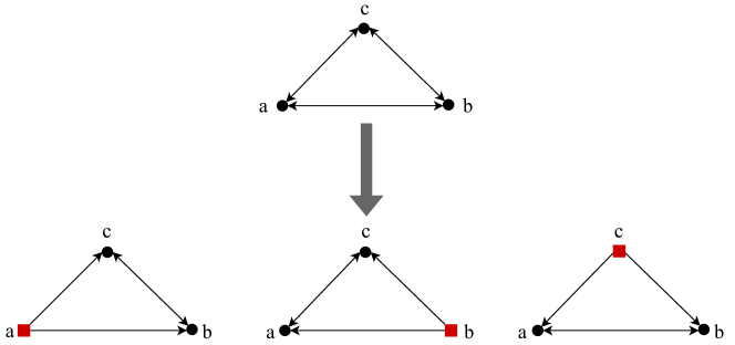
Figure 1: The localized maps for a simple TCN system.

To save transportation cost, partial outsourcing is implemented in practice to fulfill some small demands with long OD distance. To specify the destinations using partial outsourcing, we propose a two-layer graph for the localized package shipment problem with partial outsourcing, where the packages for the destination centers in first layer are shipped by the origin transit center itself, and those for destinations in the second layer are shipped by partial outsourcing.

Two-Layer Graph We take a simple example to illustrate the constructed two-layer graph for the LPS-TCN model. Given an origin center and a set of destination centers in the LPS-TCN, the packages must be shipped from the origin to each destination to meet its demand, see Figure 2, where $o$ is the origin center and others are destinations.

The origin center generally transports packages by sending vehicles on its own, e.g., $o\rightarrow d$ or $o\rightarrow c\rightarrow d$ in Figure 2. However, it might be uneconomical to directly ship packages to a destination with a long distance and a small amount of packages, e.g., $z_{2}$. In this case, the origin partially outsources the shipment to some centers. For example, $o$ can utilize the partial outsourcing to ship packages to transit center $z_{2}$ via $c$ or $d$ or both, i.e., it first ships packages for $z_{2}$ to transit center $c$ or $d$ or both, and then resorts to $c$ or $d$ or both to ship these packages to $z_{2}$ later.

The partial outsourcing decides how to split the demand and how to ship the split demands to assigned transit centers, e.g., if $o$ resorts to $c$ and $d$ to ship packages to $z_{2}$, which paths should $o$ choose to ship the packages, the $o\rightarrow c$, $o\rightarrow d$ or $o\rightarrow c\rightarrow d$? Hence, the outsourcing and route decisions are highly entangled with each other, leading to a complicated problem.

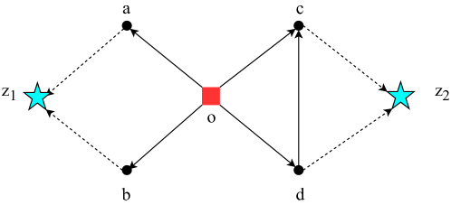
Figure 2: The Transit Center Network for packages and vehicles.

To deal with this challenge, we construct a novel two-layer graph (Figure 3) for the LPS-TCN in Figure 2, where one layer contains the origin and destination transit centers whose packages shipped by the origin itself, e.g, $a,b,c$ and $d$, and the other layer contains destinations whose packages are shipped by partial outsourcing, i.e., $z_{1}$ and $z_{2}$, and dotted lines between two layers indicate that the two centers are connected, e.g. $d\dashrightarrow z_{2}$.

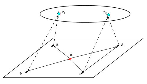
Figure 3: The two-layer graph for the TCN in Figure 2.

3.2 Notation

We introduce the notation used throughout the paper. Let $\mathbb{R}$, $\mathbb{R}_{+}$, and $\mathbb{Z}_{+}$ denote the sets of real numbers, non-negative real numbers, and non-negative integers, respectively. For any $I\in\mathbb{Z}_{+}$, we use $[I]$ to denote the set $\{1,2,\cdots,I\}$. A two-layer network $\mathcal{G}$ is represented as a directed graph $\mathcal{G}=(\mathcal{V},\mathcal{A})$, with the origin center $o$, each node in $\mathcal{V}$ representing a destination transit center, and each arc in $\mathcal{A}$ representing a link between two centers, i.e., these centers are connected. Packages are shipped by heterogeneous vehicles with available vehicle types $\mathcal{K}$. For each $k\in\mathcal{K}$, let $q_{k}$ be the capacity of type $k$ vehicles and $c_{k}$ be the cost of type $k$ vehicles per kilometer. The set $\mathcal{V}=\mathcal{V}^{1}\cup\mathcal{V}^{2}$ contains the destination centers in first layer represented as $\mathcal{V}^{1}$ and the ones in the second layer represented as $\mathcal{V}^{2}$. Similarly, the arc set $\mathcal{A}=\mathcal{A}^{1}\cup\mathcal{A}^{2}$ also contains two parts, i.e., the set $\mathcal{A}^{1}=\{(i,j)~{}|~{}i\in\mathcal{V}^{1}\cup\{o\},~{}j\in\mathcal{V}^{1}\}$ representing arcs in the first layer and $\mathcal{A}^{2}=\{(i,j)~{}|~{}i\in\mathcal{V}^{1},~{}j\in\mathcal{V}^{2}\}$ representing arcs between the first and second layer. Let $\mathcal{P}$ denote the set of feasible paths in the fist layer, i.e. the path with limited number of arcs in view of the practical restriction. For each $i\in\mathcal{V}^{1}$, let $\mathcal{P}_{i}\subseteq\mathcal{P}$ be the set of paths that go through node $i$. For each $i\in\mathcal{V}$, let $\mathcal{N}_{i}^{+}=\{j\in\mathcal{V}~{}|~{}(i,j)\in\mathcal{A}\}$ and $\mathcal{N}_{i}^{-}=\{j\in\mathcal{V}\cup\{o\}~{}|~{}(j,i)\in\mathcal{A}\}$ be the sets of out-neighbors and in-neighbors of $i$, $d_{i}$ be the predicted demand of $i$, and $\mathcal{D}=\{d_{i}~{}|~{}i\in\mathcal{V}\}$ be the set of demands of all node. For each $a=(i,j)\in\mathcal{A}^{1}$, $\mathcal{P}_{a}\subseteq\mathcal{P}$ denotes the set of feasible paths containing arc $a$, $l_{a}$ $(l_{ij})$ is the length of arc $a=(i,j)$. And $x_{a}$ $(x_{ij})\in\mathbb{R}_{+}$ is a continuous decision variable deciding the amount of packages on arc $a=(i,j)\in\mathcal{A}$. For each arc $(i,j)\in\mathcal{V}^{2}$, $c_{ij}^{\prime}$ is the unit outsourcing cost for shipping packages by transition center $i$ to destination $j$. The unit is for per cubic meter (in terms of volume) of packages and per kilometer distance traveled. For each path $p\in\mathcal{P}$ and $k\in\mathcal{K}$, $y_{p}^{k}\in\mathbb{Z}_{+}$ is the integer variable that decides the number of vehicles of type $k$ used on path $p$. For the sake of readability, we summarize the notation in Table 1.

Table 1: Notation

Category	Notation	Description
Set	$\mathcal{K}$	Set of vehicle types
	$\mathcal{P}$	Set of feasible paths to each destination $i\in\mathcal{V}^{1}$
	$\mathcal{P}_{i}$	Set of feasible paths containing transit center $i\in\mathcal{V}^{1}$
	$\mathcal{P}_{a}$	Set of feasible paths containing arc $a$
	$\mathcal{V}^{1}$	Set of destination centers in the first layer
	$\mathcal{V}^{2}$	Set of destination centers in the second layer
	$\mathcal{V}$	$\mathcal{V}:=\mathcal{V}^{1}\cup\mathcal{V}^{2}$
	$\mathcal{A}^{1}$	Set of arcs in the first layer
	$\mathcal{A}^{2}$	Set of arcs between the first and second layer
	$\mathcal{A}$	$\mathcal{A}:=\mathcal{A}^{1}\cup\mathcal{A}^{2}$
	$\mathcal{N}^{+}_{i}$	Set of out-neighbors of center $i$
	$\mathcal{N}^{-}_{i}$	Set of in-neighbors of center $i$
	$\mathcal{D}$	Set of demands
Parameter	$l_{a}$ $(l_{ij})$	Length of arc $a=(i.j)\in\mathcal{A}$
	$q_{k}$	Capacity of type $k\in\mathcal{K}$ vehicle
	$d_{i}$	Predicted demand of destination $i\in\mathcal{V}$
	$c_{k}$	Unit cost of type $k$ vehicle (per kilometer).
	$c^{\prime}_{ij}$	Unit outsourcing cost from $j$ to $i$ (per cubic meter
		and per kilometer)
Decision Variable	$y_{p}^{k}\in\mathbb{Z}_{+}$	Number of type $k\in\mathcal{K}$ vehicles that use path $p\in\mathcal{P}$
	$x_{a}$ $(x_{ij})\in\mathbb{R}_{+}$	Amount of packages transported on arc $a=(i,j)\in\mathcal{A}$

3.3 The Two-layer LPS-TCN Model

Let $G=(\mathcal{V},\mathcal{A})$ be the two-layer graph with the origin node $o$, the LPS-TCN model can be formulated as the following MIP.

min $$\sum_{a\in\mathcal{A}^{1}}\sum_{p\in\mathcal{P}_{a}}\sum_{k\in\mathcal{K}}c_{k}l_{a}\cdot y_{p}^{k}+\sum_{(i,j)\in\mathcal{A}^{2}}c^{\prime}_{ij}l_{ij}\cdot x_{ij}$$ (1a)

$$\operatorname*{s.t.} \sum_{j\in\mathcal{N}_{i}^{+}}x_{ij}-\sum_{j\in\mathcal{N}_{i}^{-}}x_{ji}=w_{i},~{}~{}\forall i\in\mathcal{V}\cup{\{o\}},$$ (1b)

$$\sum_{k\in\mathcal{K}}\sum_{p\in\mathcal{P}_{a}}q_{k}y_{p}^{k}\geq x_{a},~{}~{}\forall a\in\mathcal{A}^{1},$$ (1c)

$$x_{a}\geq 0,~{}~{}\forall a\in\mathcal{A},$$ (1d)

$$y_{p}^{k}\in\mathbb{Z}_{+},~{}\forall p\in\mathcal{P},~{}~{}\forall k\in\mathcal{K},$$ (1e)

where $w_{i}=\sum_{i\in\mathcal{V}}d_{i}$ if $i=o$, and $w_{i}=-d_{i}$ if $i\in\mathcal{V}$.

Given the set $\mathcal{P}$ of feasible paths in the first layer, the proposed LPS-TCN model in (1) seeks to find vehicle routes and package flows that achieve the minimum cost, which is computed in the objective function (1a) as a sum of the transportation cost in the first layer and outsourcing cost between the two layers. Constraint (1b) results from the flow conservation and ensures the demand is satisfied for each destination center, i.e., the net package flow, computed as the difference of amount of packages flowing into the center and the amount of flowing out, equals the demand. For the origin center, it only has outgoing flow with amount equal to the sum of all demands. Constraint (1c) ensures that the total capacity of different types of vehicles is no smaller than the amount of package flow on each arc $a\in\mathcal{A}^{1}$, i.e., there is enough capacity to perform the transportation. Constraints (1d) and (1e) are non-negative and integer constraints.

3.4 The Computational Complexity of the LPS-TCN Problem

In this subsection, we show the computational complexity of the LPS-TCN Problem. First, we recall the $K$-partition problem with $K\geq 3$, which has been shown to be strongly NP-complete by Babel, Kellerer, and Kotov (1998).

$K$-PARTITION Problem $\bm{Instance.}$ Given a list $L$ of $Km$ integers $\mu_{1},\mu_{2},\dots,\mu_{Km}$ with $K\geq 3$, and a bound $B\in\mathbb{Z}_{+}$ such that $B/(K+1)<\mu_{j}<B/(K-1)$ for $j=1,\dots,Km$ and $\sum_{j=1}^{Km}\mu_{j}=KB$. $\bm{Question.}$ Can $L$ be partitioned into $m$ disjoint subsets $S_{1},\dots,S_{m}$ such that $\sum_{j\in S_{i}}\mu_{j}=B$ for $j=1,\dots,Km$ ?

We use this problem to analyze the computational complexity of our problem.

Theorem 1

The problem of deciding whether there exists a feasible transportation plan for packages and vehicles where the number of arcs for each path is no larger than a given constant $n\geq 3$ and the transportation cost is no more than a given constant $C$ is Strongly NP-complete.

The proof is included in Section A of the Online Appendix. The main idea is to show that the $K$-partition problem can be polynomially reduced to our two-layer LPS-TCN problem, i.e., the $K$-PARTITION problem can be answered by solving an instance of the LPS-TCN model.

Theorem 1 implies that problem (1) is NP-hard in the strong sense. This result is not too surprising since the number of feasible paths increases exponentially as the size of the graph grows.

4 Column Generation Based Algorithm for the LPS-TCN Model

The LPS-TCN model is defined by the set of feasible paths $\mathcal{P}$, which is typically too time-consuming to enumerate a priori. Fortunately, if a tight enough lower bound (LB) and an upper bound (UB) of model (1) are known, many paths can be eliminated from set $\mathcal{P}$ if they do not satisfy some condition on the UB and LB (Yang 2021, Proposition 4). In other words, there is no need to enumerate all paths to solve (1), which inspires us to design the following effective CG-based algorithm. We outline the whole algorithm to solve problem (1) in Algorithm 1, whose $5$ steps are detailed subsequently. By convention, the restricted master problem (RMP) in the following is referred to as the LPS-TCN model defined by the paths that has been generated so far.

Input: A small subset of feasible paths

Output: An optimal solution to the primal model (1)

Step 1. The LB Computation: Solve the Linear programming (LP) relaxation of problem (1) by CG method to get an LB and a set of paths generated in CG, denoted as $\bar{\mathcal{P}}\subseteq\mathcal{P}$

Step 2. The UB Computation: Solve the RMP defined over set $\bar{\mathcal{P}}$ by an IP solver to obtain an UB

Step 3. Path Enumeration: Add all feasible paths satisfying some condition defined by the gap UB-LB to set $\bar{\mathcal{P}}$ to obtain an enlarged set $\tilde{\mathcal{P}}$

Step 4. Algorithm Acceleration: Add modified rounded capacity cuts to RMP and tight the integer variable bounds

Step 5. Optimal Solution Computation: Solve the RMP (2) with modified cuts and tight integer variables bounds over set $\tilde{\mathcal{P}}$ by an IP solver

Algorithm 1 The algorithm for solving (1)

Algorithm 1 first applies CG method to obtain an LB by solving the LP relaxation of (1) in Step 1. Then we call an IP solver to solve the RMP over the paths generated so far to obtain UB in Step 2. In the Step 3, we subsequently enumerate paths satisfying some condition defined by the gap UB - LB. To accelerate the solution, we also add some problem specific cuts and tighten the bounds of the integer variables based on a mild assumption on the network in Step 4. Finally, in Step 5, the resulting MIP is solved directly by an IP solver to obtain an optimal solution to the original problem.

4.1 Step 1: CG Method for LB Computation

In this subsection, we detail the CG method. It starts with a small subset of paths, which includes at least one path for each destination, such that an initial feasible solution can be obtained. Let $\bar{\mathcal{P}}_{a}:={\mathcal{P}}_{a}\cap\bar{\mathcal{P}}$, then, the RMP defined by $\bar{\mathcal{P}}$ is given as

min $$\sum_{a\in\mathcal{A}^{1}}\sum_{p\in\bar{\mathcal{P}}_{a}}\sum_{k\in\mathcal{K}}c_{k}l_{a}\cdot y_{p}^{k}+\sum_{(i,j)\in\mathcal{A}^{2}}c^{\prime}_{ij}l_{ij}\cdot x_{ij}$$ (2a)

$$\operatorname*{s.t.} \sum_{j\in\mathcal{N}_{i}^{+}}x_{ij}-\sum_{j\in\mathcal{N}_{i}^{-}}x_{ji}=w_{i},~{}~{}\forall i\in\mathcal{V}\cup{\{o\}},$$ (2b)

$$\sum_{k\in\mathcal{K}}\sum_{p\in\bar{\mathcal{P}}_{a}}q_{k}y_{p}^{k}\geq x_{a},~{}~{}\forall a\in\mathcal{A}^{1},$$ (2c)

$$x_{a}\geq 0,~{}~{}\forall a\in\mathcal{A},$$

$$y_{p}^{k}\in\mathbb{Z}_{+},~{}~{}\forall p\in\bar{\mathcal{P}}.$$

Based on an optimal dual solution of the LP relaxation of the RMP problem (2), new feasible paths using different types of vehicles can be generated according to their reduced costs, which are defined as follows.

Definition 1

For the LP relaxation of the model (2), let $\pi_{a}$ be an optimal dual solution associated with the capacity constraint (2c) of arc $a\in\mathcal{A}^{1}$, the reduced cost $r^{k}$ of variable $y_{p}^{k}$, which corresponds to the path $p$ using type $k$ vehicle, is defined as $r^{k}=\sum\limits_{a\in p}(c_{k}l_{a}-q_{k}\pi_{a}).$

After solving the linear relaxation of the RMP (2), a pricing subproblem is solved to generate paths with negative reduced cost for each type of vehicles. For each type $k\in\mathcal{K}$, the subproblem can be formulated as the problem of finding the shortest path from the origin $o$ to $i\in\mathcal{V}^{1}$ with arc “distance” $(c_{k}l_{a}-\pi_{a}q_{k})$. Note that there is a limit on the number of arcs for a path to be feasible, the problem is actually a shortest path problem with resource constraints (SPPRC), which is known to be strongly NP-hard. The SPPRC is well studied and can be solved by dynamic programming methods (Bellman 1958, Ford Jr and Fulkerson 2015). We implement a dynamic programming based labeling algorithm that has been widely used in the literature (Aneja, Aggarwal, and Nair 1983, Chabrier 2006, Kergosien et al. 2021, Sadykov, Uchoa, and Pessoa 2021).

Let path $p=(o,i_{1},\dots,i_{n_{p}})$ be an elementary path that starts from the origin, i.e., $o$, visits a set of transition centers $\mathcal{V}^{p}=\{i_{1},\dots,i_{n_{p}}\}$ exactly once. We define the label used in the labeling algorithm as follows.

Definition 2

The label $L^{k}_{p}$ associated with path $p$ using type $k$ vehicles is defined to be a $4$-tuple $L^{k}_{p}:=(i_{p},r^{k}_{p},s_{p},n_{p})$, where $i_{p}:=i_{n_{p}}$ is the last transition center in path $p$, $r_{p}^{k}$ is the reduced cost for path $p$ using type $k$ vehicles, $s_{p}$ and $n_{p}$ are the length and the number of arcs of path $p$, respectively.

A label $L^{k}_{p}$ is feasible if $n_{p}\leq n$, where $n\geq 0$ is a given constant. Generating paths using type $k$ vehicles with reduced cost less than $0$ is equivalent to generating feasible labels using type $k$ vehicles with negative reduced cost, which is accomplished by the labeling algorithm. In particular, $L^{k}_{p}$ can be extend to $L^{k}_{p\prime}=(j,r_{p^{\prime}}^{k},s_{p^{\prime}},n_{p^{\prime}})$ by the following update rule, where $p^{\prime}=(o,i_{1},\dots,i_{n_{p}},j)$ for $j\in\mathcal{V}^{1}\setminus\mathcal{V}^{p}$.

$$r_{p^{\prime}}^{k}=r^{k}_{p}+c_{k}l_{i_{n_{p}}j}-\pi_{i_{n_{p}}j}q_{k}$$ (3)

$$s_{p^{\prime}}=s_{p}+l_{i_{n_{p}}j}$$

$$n_{p^{\prime}}=n_{p}+1.$$

To accelerate the labeling algorithm, we apply the dominance rule in Proposition 1.

Proposition 1 (Dominance Rule)

A label $L^{k}_{p_{1}}=(i_{p_{1}},r^{k}_{p_{1}},s_{p_{1}},n_{p_{1}})$ dominates another label $L^{k}_{p_{2}}=(i_{p_{2}},r_{p_{2}}^{k},s_{p_{2}},n_{p_{2}})$, denoted by $L^{k}_{p_{1}}\prec L^{k}_{p_{2}}$, if $(i)~{}i_{p_{1}}=i_{p_{2}}$, $(ii)~{}\mathcal{V}^{p_{1}}\subseteq\mathcal{V}^{p_{2}}$, $(iii)~{}r^{k}_{p_{1}}\leq r_{p_{2}}^{k}$, $(iv)~{}s_{p_{1}}\leq s_{p_{2}}$, and $(v)~{}n_{p_{1}}\leq n_{p_{2}}$ hold.

Each time a new label is obtained by the extension rule in (LABEL:update_rule), we first check its feasibility. Then, we check whether it is dominated by other labels that have been generated. If so, it is discarded, otherwise it is added to the label list. Lastly, we test all other labels and delete those dominated by the new one.

4.2 Step 2: The UB Computation

After solving the LP relaxation of model (1), we obtain an LB and a set of feasible paths $\bar{\mathcal{P}}$. Then, we compute an UB for (1) by solving the RMP problem (2) defined by set $\bar{\mathcal{P}}$. Due to the moderate size of $\bar{\mathcal{P}}$, which generally consists of hundreds of feasible paths, it can be solved fast by an off-the-shelf MIP solver, such as CPLEX.

4.3 Step 3: Path Enumeration

As mentioned in Section 3.4, there is no need to enumerate all feasible paths. Instead, according to Proposition 4 in Yang (2021) (the following Corollary 1), it suffices to add paths using type $k$ vehicle that have reduced costs $r_{p}^{k}$ less than UB-LB into set $\bar{\mathcal{P}}$. Consequently, the RMP model (2) based on this enlarged $\bar{\mathcal{P}}$, denoted by $\tilde{\mathcal{P}}$, can yield the same optimal solution as (1) with the set of all feasible paths $\mathcal{P}$. To enumerate all qualified paths, we adopt the Yen’s Algorithm (Yen 1971).

Corollary 1

(Yang 2021, Proposition 4) Given an LB and UB for the primal model (1), paths with reduced cost larger than UB-LB will not be in any optimal solution to (1), i.e., $y_{p}^{k}=0$ if $r_{p}^{k}\geq$ UB-LB.

4.4 Step 4: Algorithm Acceleration

To further reduce the computation time, we propose to add some problem-specific cutting planes and tighten the variable bounds by taking advantage of some problem structure.

4.4.1 The Modified Rounded Capacity Cuts

We tailor the well-known rounded capacity cuts to our problem, which ensures that the vehicles dispatched to ship packages for each destination have enough capacity to complete the shipment.

Theorem 2

The following inequality is valid for the LPS-TCN model (1)

$$\sum_{k\in\mathcal{K}}\sum_{p\in\mathcal{P}_{i}}y^{k}\geq\left\lceil\frac{d_{i}}{q^{*}}\right\rceil,~{}~{}\forall i\in\mathcal{V}^{1},$$ (4)

where $q^{*}=\max_{k\in\mathcal{K}}\{q_{k}\}$.

The proof for Theorem 2 is provided in Section B of the Online Appendix.

4.4.2 Variable Bound Tightening

We utilize the problem structure to tighten the variable bounds, which is based on the following two practical assumptions.

Assumption 1 (Connectedness)

The origin $o$ is connected to each destination center in the first layer.

In practice, for each OD demand, there is always an arc linking the origin $o$ and the corresponding destination. Thus, this assumption is always satisfied.

Assumption 2 (Triangle Inequality)

For any arc $(i,j)\in\mathcal{A}^{1}$, $l_{ij}\leq l_{ik}+l_{kj}$ holds for $\forall(i,k),(k,j)\in\mathcal{A}^{1}$.

In practice this assumption may not always be satisfied. But it is a common assumption in the context of vehicle routing and matches reality in most cases.

Let $p=(o,i_{1},\dots,i_{n_{p}})$ be a path and $\{\bar{z}^{ki_{j}}_{p}\}_{j=1}^{n_{p}}$ be the amount of packages delivered to node $i_{j}$ via path $p$ by type $k$ vehicle. Under Assumptions 1 and 2, we can tighten the variable bound by the following Theorem 3.

Theorem 3

Under Assumption 1 and 2, for any optimal solution $(\bar{x},\bar{y})$ to (1), we have $\bar{y}^{k}\leq 1$ for each $p$ with $n_{p}\geq 2$. Furthermore, $\bar{z}^{ki_{j}}_{p}\leq q_{k}$ for each node $i_{j}$ in path $p$.

Theorem 3 is proved by contradiction in Section C of the Online Appendix. The main idea is to show that if the number of type $k$ vehicles on path $p$ with $n_{p}\geq 2$ is larger than $1$, i.e., $\bar{y}_{p}^{k}>1$, we can always request one of the vehicles to travel a different path $p^{\prime}$. The result will not increase the cost and will still satisfy all the demands. More precisely, we have $\mathcal{V}^{p^{\prime}}\subset\mathcal{V}^{p}$ and $l_{p^{\prime}}\leq l_{p}$.

Without loss of generality, we assume that the capacity of vehicles $\{q_{k}\}_{k\in\mathcal{K}}$ are in an ascending order, that is, $q_{i}<q_{j},\forall~{}i\leq j,~{}i,j\in\mathcal{K}$. Under this assumption, except for the vehicle with the maximal capacity, i.e. $k=|\mathcal{K}|$, we can find an upper bound for the number of type $k$ vehicle on path $p$ with only one arc by solving an integer program.

Theorem 4

We can find an optimal solution $(\bar{x},\bar{y})$ to problem (1) such that $\bar{y}_{p}^{k}$ is no larger than the optimal value of the following integer program for each $k\in\mathcal{K}\setminus\{|\mathcal{K}|\}$ and $p$ with $n_{p}=1$.

$${\rm min.} ~{}~{}~{}~{}u_{k}$$

$${\rm s.t.} ~{}\sum_{i\in\mathcal{K},i>k}c_{i}v_{i}\leq c_{k}u_{k}$$ (5a)

$$~{}\sum_{i\in\mathcal{K},i>k}q_{i}v_{i}\geq q_{k}u_{k}$$ (5b)

$$~{}u_{k}\in\mathbb{Z}_{+},~{}v_{i}\in\mathbb{Z}_{+},\forall i\in\mathcal{K},i>k,$$

where $u_{k}$ is an integer variable counting the number of type $k$ vehicle on path $p$, $v_{i}$ is the integer variable counting the number of type $i\in\mathcal{K},i>k$ vehicle on path $p$. The constraint (5a) requires to find a group of vehicles with capacity larger than $q_{k}$ such that their total cost is no larger than $c_{k}u_{k}$. Constraint (5b) requires that the total capacity of this group is no less than $q_{k}u_{k}$.

Theorem 4 is proved in Section D of the Online Appendix. Note that problem $\eqref{add_bound}$ depends only on the vehicle type, and thus the number of type $k$ vehicles on different path $p$ has the same upper bound. Hence, we only need to solve $|\mathcal{K}|$ problems to obtain all upper bounds for $y$ variables. Generally, the number of the vehicle types is small and the problem (5) is easily solved by an IP solver.

4.5 Step 5: Optimal Solution Computation

We have enumerated all necessary paths (columns), added problem specific cuts to the proposed model, and tightened the bounds of integer variables. The resulting MIP can be solved directly to obtain an optimal solution to the original problem. In this step, we adopt one of the state-of-the-art MIP solvers CPLEX to compute an optimal solution to problem (1).

5 Numerical Results

In this section, we illustrate the superiority of the CG-based Algorithm 1 compared with CPLEX’s default method and test the performance of the proposed LPS-TCN model using real-world instances. The code is implemented in C++ and all experiments are performed on a workstation running Ubuntu 20.04 with AMD Ryzen Threadripper 3990X 64-core, 128-thread processor and 128 GB RAM. CPLEX 12.8 is employed to solve the involved MIP and LP models. We limit the number of arcs on feasible paths to $3$, which is consistent with the path limitation in a major Chinese package express company.

Table 2: Selected origin transit centers

Scale	City
Small	Fuyang, Zigong, Tianjin, Luoyang, Taizhou, Wuhu, Bengbu, Changchun,
	Liuzhou, Guiyang
Middle	Fuzhou, Shengyang, Linhai, Haerbin, Kunming
Large	Wenzhou, Shanghai, Wuhan, Beijing, Zengcheng

The raw data used in our experiments comes from a major Chinese package express company and has been desensitized for data security. In total, there are $20$ instances generated by the following steps. $1)$ Select $20$ transit centers as origins, which contain $10$ small-scale, $5$ middle-scale, and $5$ large-scale centers; $2)$ Build the corresponding two-layer graph for the LPS-TCN based on the “Current-Next-Final” (CNF) network provided by the company, where $C$ is one of the selected origins, $N$ is the set of next centers to which the packages are shipped, $F$ is the set of final center for packages. We set the $N$ centers as destination nodes in the first layer and $F$ centers as destination nodes in the second layer. Moreover, the origin is connected with each destination centers in the first layer and if the distance between two destination centers in the first layer is less than a given constant, e.g., $500$km, these centers are connected by arcs. Then, we obtain a two-layer graph for the proposed LPS-TCN model. $3)$ We collect package flows on the CNF network for each of the $20$ origins in the LPS-TCN over a week spanning from September 13, 2021 to September 19, 2021. The OD demands are calculated by package flows. Consequently, we have $20*7=140$ different two-layer graphs for our LPS-TCN models.

Remark 1

Figure 4 is an example that illustrates step $2$, where the red parallelogram is current center, triangles are next centers and hexagons are final centers. We transform the CNF network to a two-layer graph, i.e., set the triangles as destination centers in the first layer and hexagons as centers in the second layer. Moreover, as the distance between $N_{2}$ and $N_{3}$ is less than $500$km, they are connected in the two-layer graph.

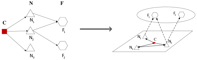
Figure 4: The CNF network and the corresponding two-layer graph for the LPS-TCN model.

There are 4 vehicle types, i.e., $\mathcal{K}=\{1,2,3,4\}$, in our experiments, and the corresponding parameters used are summarized in Table 3. The distance between transit centers are captured from the AMAP which provides a live traffic data interface.

Table 3: Parameters Setting

Parameter	Setting
$q_{k}$	$q_{1}=65,q_{2}=90,q_{3}=130,q_{4}=175$, with unit $\text{m}^{3}$
$c_{k}$	$c_{1}=4.1,c_{2}=4.7,c_{3}=6.5,c_{4}=7.5$, with unit CNY/km
$c^{\prime}_{ij}$	$0.06$ with unit $\text{CNY}/(\text{km}\cdot\text{m}^{3})$

5.1 The Optimal Vehicle Routes in Different Transit Centers

Figure 5 shows the vehicle route decisions of the proposed LPS-TCN model for two different origins, where “Luoyang” is a small-scale origin transit center and “Wuhan” is a large-scale one. The red stars and dots represent the origin and destination centers, respectively. The gray, blue, and purple lines indicate that the paths have one, two, and three arcs respectively.

We can observe from Figure 5 that the number of paths with one arc (gray lines) is the largest, which indicates that most vehicles are responsible for single shipments, i.e., the vehicle only ships the packages to one destination. Moreover, the optimal routes obtained by our model match the true situation.

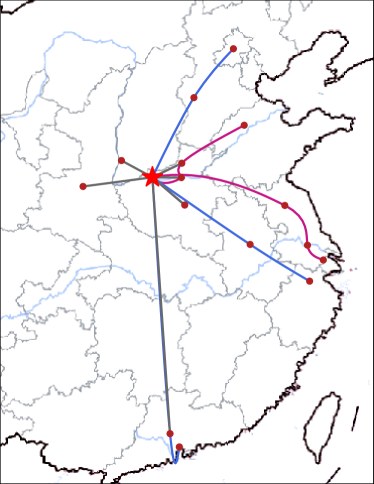
(a) Illustration of vehicle routes for Luoyang transit center.

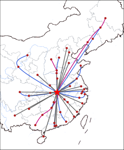
(b) Illustration of vehicle routes for Wuhan transit center.

Figure 5: The vehicle routes in different transit centers

5.2 Performance of the Proposed LPS-TCN Model

Numerical experiments on the aforementioned $20$ instances are conducted to evaluate the performance of the proposed LPS-TCN model. We first compare the averaged transportation costs over $7$ days of the LPS-TCN model with the averaged real costs. Then, we compare the cost of the two-layer graph LPS-TCN model with that of a transportation plan which also takes advantage of partial outsourcing. The purpose of the second set of experiments is to verify that in addition to partial outsourcing, the optimization of package flows and vehicle routes also help to drive the transportation cost down.

Remark 2

Although the collected data does not provide the real transportation cost directly because it does not include vehicle routes, we can derive them by solving an integer program based on the given package flows. Consequently, we obtain the true transportation cost.

Remark 3

The additional transportation plan with outsourcing is derived as follows. We start from the LPS-TCN model over the two-layer graph constructed from the CNF network, and fix its package flows according to the real plan. Then, we derive vehicle routes in the first layer based on the fixed package flows and assume that the packages to centers in the second layer are handled by partial outsourcing. Thus, the transportation cost can be computed accordingly.

Results are reported in Figure 6, where “Real Cost” represents the true transportation cost, “Revised Cost” is the cost of the derived transportation plan based on fixed package flows, and “Model Cost” is the objective value of the best solution to the LPS-TCN model at termination.

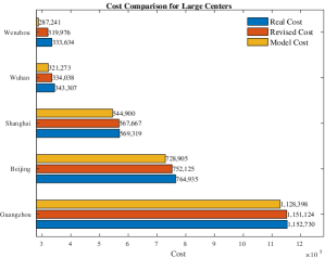
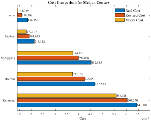
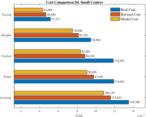
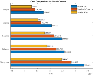
Figure 6: Averaged cost (CNY) of different methods

From Figure 6, one can observe that our LPS-TCN model yields solutions that bring significant economic benefits, i.e., a daily cost reduction up to tens of thousands of CNY for each transit center. Consequently, the daily cost reduction for the whole TCN with hundreds of transit centers is more than one million CNY. An interesting observation is that the cost reduction depends on the scale of transit center and the larger the center, the smaller the cost reduction. The intuition behind is that large-scale transit centers generally have large OD demands and tend to ship most of the packages by themselves. Hence, the packages to be partially outsourced is smaller, which leads to a smaller cost reduction. Figure 6 also shows that the LPS-TCN model exhibits better performance in terms of the transportation cost than the derived transportation plan with outsourcing, which indicates that our proposed model can additionally provide better package and vehicle routes. In summary, our LPS-TCN model can reduce the costs not only by providing better routes for packages and vehicles but also by taking advantage of partial outsourcing.

5.3 Performance Analysis of the CG-based Algorithm

The goal of this subsection is to perform a comprehensive comparison of our CG-based algorithm and the CPLEX’s default method. Experiments on real instances for different origins with scale parameters ($\mathcal{V}^{1}$, $\mathcal{V}^{2}$) over seven days are conducted. The $(D^{1},D^{2})$ denotes the total demands in the first and second layer respectively. The computation is terminated once the CPU time reaches 1,800 seconds (half an hour).

Table LABEL:tab:cplex reports the average computational time (Time), the optimality gap at termination (Gap), and the percentage of instances solved to optimality within the time limit (Opt), where the first two metrics are averaged over seven instances. Columns “CPLEX” and “CG” represent the performance of CPLEX’s default method and the proposed CG-based method respectively.

Table 4: Performance analysis of the CG-based algorithm

Origins	$\mathcal{V}^{1}$	$\mathcal{V}^{2}$	$D^{1}$	$D^{2}$	Time		Gap		Opt
					CPLEX	CG	CPLEX	CG	CPLEX	CG
Fuyang	7	103	333	595	0.77	0.57	0	0	100%	100%
Zigong	11	108	622	1,217	0.30	0.24	0	0	100%	100%
Tianjin	15	104	721	1,232	1.95	1.30	0	0	100%	100%
Luoyang	17	104	737	1,178	12.78	8.62	0	0	100%	100%
Taizhou	15	102	970	1,003	62.90	56.08	0	0	100%	100%
Fuzhou	19	100	1,675	1,585	21.76	14.34	0	0	100%	100%
Bengbu	19	98	1,255	748	30.14	22.69	0	0	100%	100%
Changchun	23	100	1,192	1,246	36.86	26.09	0	0	100%	100%
Shenyang	23	100	2,112	2,324	24.21	15.97	0	0	100%	100%
Guiyang	25	90	1,177	1,297	52.07	29.14	0	0	100%	100%
Wuhu	22	92	1,682	868	291.15	147.21	0	0	100%	100%
Liuzhou	29	91	2,191	1,047	100.77	40.42	0	0	100%	100%
Linhai	30	92	1,436	910	116.53	88.78	0	0	100%	100%
Haerbin	28	96	3,075	1,569	117.06	75.16	0	0	100%	100%
Kunming	33	86	3,753	2,645	1,583.68	1,200.48	0.33%	0.21%	14%	42%
Wenzhou	52	73	3,859	1,121	1,357.16	650.56	0.04%	0.01%	42%	86%
Shanghai	66	58	12,550	1,532	1,800	1,575.64	0.25%	0.09%	0	14%
Wuhan	48	76	7,707	1,736	1,800	1,800	0.67%	0.50%	0	0
Beijing	66	59	13,517	1,808	1,800	1,800	0.49%	0.29%	0	0
Zengcheng	69	57	13,518	1,621	1,800	1,800	0.39%	0.32%	0	0

As shown in Table LABEL:tab:cplex, the average computational time of the CG-based Algorithm 1 is generally much smaller than that of CPLEX. In particular, for small and middle-scaled instances, the computational time of Algorithm 1 is only 50% of that of CPLEX. For those instances that cannot be solved within the time limit, Algorithm 1 achieves a significantly smaller optimality gap. For example, when the origin is Wuhan, although both algorithms fail to obtain an optimal solution, the Gap of Algorithm 1 is smaller than that of CPLEX; when the origin is Wenzhou, CPLEX only solves three instances to optimality, while Algorithm 1 proves optimality for six of the seven instances.

5.4 Sensitivity Analysis

As mentioned in Section 1, we should place centers with small demands and meanwhile large OD distances in the second layer to facilitate cost saving. The corresponding thresholds for demands and OD distances can affect the solution quality. In this subsection, we test the impact of such thresholds (decided by the ratio $0\leq\theta\leq 1$) on our two-layer LPS-TCN model. Details of the experiments are summarized as follows. We first select three small-scale origin centers, three middle-scale ones, and another three large-scale ones, as test instances. For each origin, we sort its OD demands in an ascending order and OD distances in a descending order. Then, the destination centers with OD demands and distances ranking within the top $\theta$ are selected as nodes in the second layers and the others are placed in the first layers. The threshold $\theta$ tested are from $\{0.9,0.8,0.7,0.6,0.5,0.4\}$.

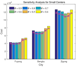
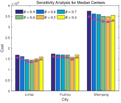
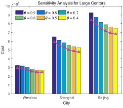
Figure 7: The sensitivity analysis for cities in different sizes

Results for different $\theta$ are presented in Figure 7. It is observed that for centers of small and middle scale, the cost first decreases and then increases as the value of $\theta$ decreases. For large centers, the cost decreases monotonically as $\theta$ decreases. In particular, we observe that the optimal threshold increases as the scale of origins increases, which is consistent with the observation in Section 5.2, i.e., the larger the origin, the higher percentage of packages shipped by the origin itself. As a result, the threshold of our two-layer LPS-TCN model should be selected based on the size of the origin center for better cost saving.

6 Conclusion

We propose a novel two-layer LPS-TCN model that emphasizes cost saving. We formulate the LPS-TCN as an MIP and prove its strong NP-hardness. To solve this model, we develop a CG-based algorithm and further enhance it by some problem-specific cutting planes and variable bound tightening techniques. Experiments on realistic instances demonstrate that the LPS-TCN can yield solutions with significant economic benefits. Moreover, the proposed algorithm significantly outperforms the CPLEX solver in terms of the computation time.

In the future, highly effective algorithms can be studied to tackle large-scale instances of the proposed LPS-TCN model. Moreover, as there exists prediction error in the predicted next-day demand, a model considering uncertain next-day demand can be studied to propose a more reliable transportation plan. In particular, distributionally robust optimization techniques can be applied to address the uncertainty, which exhibits good out-of-sample performance and has been applied to different fields, such as portfolio optimization, appointment scheduling problems, and shortest path problems.

Online Appendix: Proofs

A Proof of Theorem 1

Proof.

Proof The problem defined in Theorem 1 is the decision version of the proposed LPS-TCN problem, we denote it as D(LPS-TCN). The proof is based on the reduction from the well-known NP-complete $K$-PARTITION problem to our LPS-TCN problem.

We show that any instance $I$ of $K$-PARTITION Problem can be polynomially transformed into an equivalent instance $I^{\prime}$ of D(LPS-TCN) by setting $n=K$. The instance $I^{\prime}$ of our problem has an origin center $o$ and a set of destination nodes $\mathcal{V}^{1}=\{1,\dots,Km\}$ in the first layer. The demand of each destination $i\in\mathcal{V}^{1}$ is equal to $\mu_{i}$. The arc set is $\mathcal{A}^{1}=\{(i,j)~{}|~{}i\in\mathcal{V}^{1}\cup\{o\},j\in\mathcal{V}^{1}\setminus\{i\}\}$. There is only one vehicle type with capacity $B$, unit cost per kilometer traveled, and no destination center in the second-layer, i.e., $|\mathcal{K}|=1,\mathcal{V}^{2}=\emptyset$. Lastly, we assume that all destinations are evenly distributed on a circular arc centered at the origin center with a radius $R$ and a radian. The radian is small enough such that the chord between any destinations are bounded by a given constant $U_{b}={R}/{Km}$. Then, the cost of vehicles on arc $(i,j)\in\mathcal{A}^{1}$ equals $R$ if $i=o$ and others equals $l_{ij}\leq U_{b}$. Finally, we set the total cost $C$ to $mR+(K-1)mU_{b}$.

We first prove that the given cost $C$ bounds the number of vehicles used to ship packages to be no more than $m$. Actually, the number of vehicles in any “YES” instance of D(LPS-TCN) must be $m$, each of which is fully loaded. It can be proved by contradiction as follows.

If the number of vehicles is smaller than $m$, the capacity is less than $mB$, which is insufficient because the total demand is $\sum_{i=1}^{Km}\mu_{i}=mB$. If it is larger than $m$, then the cost $C^{\prime}\geq(m+1)R$. However,

$$C=mR+(K-1)mU_{b}<mR+(K-1)m*\frac{R}{Km}<(m+1)R\leq C^{\prime},$$

which completes the proof. The transportation cost $C^{\prime\prime}$ of a transportation plan using $m$ vehicles is

$$C^{\prime\prime}=\sum_{p=1}^{m}l_{p}\leq mR+m\cdot(K-1)U_{b}=C,$$

where $l_{p}$ is the length of path $p$ used by vehicle $p$. The inequality holds when the number of arcs of each path is no larger than $K$ and the length of each arc is bounded by $U_{b}$.

Next, we prove that in any “YES” instance of D(LPS-TCN), all demands must be shipped without split, i.e., the demand of each destination is shipped completely by one vehicle. Again, this can be proved by contradiction. Without loss of generality, assume there exists a destination $d$ whose demand is shipped by two vehicles, denoted by $k$ and $j$ and all the other demands are shipped without split. For the other $m-2$ vehicles, since $B/(K+1)<\mu_{i}<B/(K-1)$, the number of destinations visited by each vehicle is exactly $K$. Thus, the total number of destinations visited by $k$-th and $j$-th vehicles is $1+Km-K(m-2)=2K+1$, as the node $d$ is visited twice. Hence, there must be a vehicle, either $k$ or $j$, that visits more than $K$ nodes, which is infeasible in our problem due to the limit on the length of path. Consequently, the constructed instance of D(LPS-TCN), $I^{\prime}$, has to find a partition of destinations denoted by $\mathcal{V}^{1}_{1},\dots,\mathcal{V}^{1}_{m}$ such that $\sum_{i\in\mathcal{V}^{1}_{j}}\mu_{i}=B$, which is exactly the decision problems for $K$-PARTITION problem. Hence, if we can find a feasible transportation plan for the LPS-TCN problem, then the instance of $K$-PARTITION problem is a YES-instance, otherwise, the instance of $K$-PARTITION problem is a NO-instance.

∎

B Proof of Theorem 2

Proof.

Proof The amount of packages transported to the destination center $i$ is no smaller than $d_{i}$. Actually, it equals $d_{i}$ if no packages for the second layer have been shipped to $i$ when partial outsourcing is allowed. Thus, the smallest number of the vehicles for destination $i$ is $\left\lceil\frac{d_{i}}{q^{*}}\right\rceil$, where only the vehicle type with the maximal capacity is used. ∎

C Proof of Theorem 3

Proof.

Proof

For the ease of exposition, we omit index $k$, i.e. the type of vehicles in this proof. Let path $p=(o,i_{1},\dots,i_{n_{p}})$ be an elementary path with $n_{p}\geq 2$, that starts from the origin, i.e., $o$, and visits a set of destination centers $\{i_{1},\dots,i_{n_{p}}\}$. We first show that for any path $p$ with $n_{p}\geq 2$ and $\bar{y}_{p}>0$ in an optimal solution, the amount of packages delivered to each node in $\{i_{1},\dots,i_{n_{p}}\}$ by path $p$, denoted by $\{\bar{z}_{p}^{i_{j}}\}_{j=1}^{n_{p}}$, is no more than $q$. It can be proved by contradiction as follows.

Note that the amount of packages delivered to any node on path $p$ is strictly positive. Otherwise, if there exists a node $i_{l}\in\{i_{1},\dots,i_{n_{p}}\}$ with $\bar{z}_{p}^{i_{l}}=0$, then the path can be shortened to $p^{\prime}=(o,i_{1},\cdots,i_{l-1},i_{l+1},\dots,i_{n_{p}})$ which has a smaller cost than path $p$. As a result, the path $p$ which contains a node with $\bar{z}_{p}^{i_{j}}=0$ is not in an optimal solution in this case.

If there exists a node $i_{l}\in\{i_{1},\dots,i_{n_{p}}\}$ with $\bar{z}_{p}^{i_{l}}>q$, we have $\bar{y}_{p}>1$, otherwise the capacity of this path is no more than $q$, which is insufficient because the total amount of package is $\sum_{j=1}^{n_{p}}\bar{z}_{p}^{i_{j}}>q$, the inequality holds as $\bar{z}_{p}^{i_{j}}>0,~{}\forall i_{j}\in\{i_{1},\dots,i_{n_{p}}\}$. Then we can derive another solution with a smaller cost. This solution contains two paths, i.e., $p$ given before and $p^{\prime\prime}=(o,i_{l})$. The notations $\hat{y}_{p}$ and $\bar{y}_{p^{\prime\prime}}$ count the number of vehicles on path $p$ and $p^{\prime\prime}$ respectively. The scalars $\{\hat{z}_{p}^{i_{j}}\}_{j=1}^{n_{p}}$ and $\{\bar{z}_{p^{\prime\prime}}^{i_{l}}\}$ denotes the amount of packages shipped to node on different paths.

Let $\bar{y}_{p^{\prime\prime}}=\left\lfloor{\bar{z}_{p}^{i_{l}}}/{q}\right\rfloor$ and $\hat{y}_{p}=\bar{y}_{p}-\bar{y}_{p^{\prime\prime}}$. Moreover, set $\bar{z}_{p^{\prime\prime}}^{i_{l}}=\left\lfloor{\bar{z}_{p}^{i_{l}}}/{q}\right\rfloor q$, $\hat{z}_{p}^{i_{l}}=\bar{z}_{p}^{i_{l}}-\left\lfloor{\bar{z}_{p}^{i_{l}}}/{q}\right\rfloor q$ and $\hat{z}_{p}^{i_{j}}=\bar{z}_{p}^{i_{j}}$ for any node $i_{j}\in\{i_{1},\dots,i_{n_{p}}\}/i_{l}$.

First we prove that the solution is feasible, i.e., it satisfies that $\sum_{j=1}^{n_{p}}\hat{z}_{p}^{i_{j}}\leq\hat{y}_{p}\cdot q$ and $\bar{z}_{p^{\prime\prime}}^{i_{l}}\leq\bar{y}_{p^{\prime\prime}}\cdot q$. The second inequality is trivial due to the definition. We next prove the first inequality. We have that

$$\sum_{j=1}^{n_{p}}\hat{z}_{p}^{i_{j}}=\sum_{j=1}^{n_{p}}\bar{z}_{p}^{i_{j}}-\left\lfloor\frac{\bar{z}_{p}^{i_{l}}}{q}\right\rfloor\cdot q\leq\bar{y}_{p}\cdot q-\left\lfloor\frac{\bar{z}_{p}^{i_{l}}}{q}\right\rfloor\cdot q=(\bar{y}_{p}-\bar{y}_{p^{\prime\prime}})q=\hat{y}_{p}\cdot q$$

where the first inequality holds due to the fact $\sum_{j=1}^{n_{p}}\bar{z}_{p}^{i_{j}}\leq\bar{y}_{p}\cdot q.$ Hence, the constructed solution is feasible.

Then we prove that the solution has a less cost than that of the primal solution. Let $c_{new}$ be the cost of this new solution, we have

$$c_{new}=l_{oi_{l}}\cdot\bar{y}_{p^{\prime\prime}}\cdot c+l_{p}\cdot\hat{y}_{p}\cdot c=l_{oi_{l}}\cdot\bar{y}_{p^{\prime\prime}}\cdot c+l_{p}\cdot(\bar{y}_{p}-\bar{y}_{p^{\prime\prime}})\cdot c=l_{p}\cdot\bar{y}_{p}\cdot c-(l_{p}-l_{oi_{l}})\cdot\bar{y}_{p^{\prime\prime}}\cdot c<l_{p}\cdot\bar{y}_{p}\cdot c,$$

where the last inequality holds due to Assumption 1 and 2, i.e.

$$l_{oi_{l}}<l_{oi_{l-1}}+l_{i_{l-1}i_{l}}<l_{{oi_{l-2}}}+l_{i_{l-2}i_{l-1}}+l_{i_{l-1}i_{l}}<\cdots<l_{oi_{1}}+l_{i_{1}i_{2}}+\cdots+l_{i_{l-1}i_{l}}\leq l_{p}.$$ (6)

Then we complete the proof.

Next we prove another part of Theorem 3 by induction on $n_{p}$, i.e. the value of integer variables $\bar{y}_{p}\leq 1$ for path with $n_{p}\geq 2$ in an optimal solution.

Step 1:

We first show that the statements holds for the smallest number $n_{p}=2$. Let $p=(o,i_{1},i_{2})$ be the path.

Note that we always have $\bar{z}^{i_{1}}_{p}<q$ and $\bar{z}^{i_{2}}_{p}<q$. Then we prove Theorem 3 by contradiction. Assume that $\bar{y}_{p}>1$ in an optimal solution. As $\bar{z}^{i_{1}}_{p}<q$ and $\bar{z}^{i_{2}}_{p}<q$, we have $\bar{z}^{i_{1}}_{p}+\bar{z}^{i_{2}}_{p}<2q$, consequently, $\bar{y}_{p}=2$. Without loss of generality, assume that $\bar{z}^{i_{1}}_{p}<\bar{z}^{i_{2}}_{p}$. Then we can use one vehicle to transport packages to ${i_{1}}$ with number being $\bar{z}^{i_{1}}_{p}$ and ${i_{2}}$ with $q-\bar{z}^{i_{1}}_{p}$ by path $p$, and use another one vehicle to transport packages to $i_{2}$ with number being $\bar{z}^{i_{2}}_{p}+\bar{z}^{i_{1}}_{p}-q$ by path $p^{\prime}=(o,i_{2})$. As a result, we have

$$c_{new} =l_{p^{\prime}}\cdot c+l_{p}\cdot c<2\cdot l_{p}\cdot c,$$

where the last inequality holds due to Assumption 2. Hence, $y_{p}>1$ is not in an optimal solution and we derive a contradiction.

Step 2: Assume that the statement holds for arbitrary natural number $n_{p}=n$.

Step 3: In this step we prove that the statement holds for $n_{p}=n+1$, i.e., the path $p=(o,i_{1},\cdots,i_{n},i_{n+1})$.

Assume that $\bar{y}_{p}>1$ in an optimal solution. As $\bar{z}^{i_{n+1}}_{p}<q$, if $\sum_{j=1}^{n}\bar{z}^{i_{j}}_{p}<q$, we have $\sum_{j=1}^{n}\bar{z}^{i_{j}}_{p}+\bar{z}^{i_{n+1}}_{p}<2q$, consequently, $\bar{y}_{p}=2$. Without loss of generality, assume that $\sum_{j=1}^{n}\bar{z}^{i_{j}}_{p}<\bar{z}^{i_{n+1}}_{p}$. We prove that we can derive another solution with a less cost. This solution contains two paths, i.e., $p$ given before and $p^{\prime}=(o,i_{n+1})$. The $\hat{y}_{p}$ and $\bar{y}_{p^{\prime}}$ count the number of vehicles on path $p$ and $p^{\prime}$ respectively. The $\{\hat{z}_{p}^{i_{j}}\}_{j=1}^{n+1}$ and $\{\bar{z}_{p^{\prime}}^{i_{n+1}}\}$ denote the amount of packages shipped to node on different paths.

Let $\bar{y}_{p^{\prime}}=1$ and $\hat{y}_{p}=1$. Moreover, set $\hat{z}_{p}^{i_{j}}=\bar{z}_{p}^{i_{j}}$ for $i_{j}\in\{i_{1},\dots,i_{n}\}$, $\hat{z}_{p}^{i_{n+1}}=q-\sum_{j=1}^{n}\bar{z}_{p}^{i_{j}}$ and $\bar{z}_{p^{\prime}}^{i_{n+1}}=\bar{z}_{p}^{i_{n+1}}-\hat{z}_{p}^{i_{n+1}}$. Obviously, this solution is feasible, that is, it satisfies that $\sum_{j=1}^{n+1}\hat{z}_{p}^{i_{j}}\leq q$ and $\bar{z}_{p^{\prime}}^{i_{n+1}}=\bar{z}_{p}^{i_{n+1}}-\hat{z}_{p}^{i_{n+1}}\leq q$.

Let $c_{new}$ denote the cost of the constructed solution, it follows that

$$c_{new} =l_{p^{\prime}}\cdot c+l_{p}\cdot c<2l_{p}\cdot c,$$

where the last inequality holds due to Assumption 1 and 2, see (6) for details. Hence, $y_{p}>1$ is not in an optimal solution in this case.

If $\sum_{j=1}^{n}\bar{z}^{i_{j}}_{p}\geq q$, we can also find a feasible solution with a less cost than current solution. It contains the given path $p$ and a different path $p^{\prime\prime}=(o,i_{1},\dots,i_{n})$. Similar to the proof in the first case, we have decision variables $\bar{y}_{p^{\prime\prime}}$, $\hat{y}_{p}$, $\{\bar{z}^{i_{j}}_{p^{\prime\prime}}\}_{j=1}^{n}$ and $\{\hat{z}^{i_{j}}_{p}\}_{j=1}^{n+1}$.

Let $\bar{y}_{p^{\prime\prime}}=\left\lfloor{\sum_{j=1}^{n}\bar{z}^{i_{j}}_{p}}/{q}\right\rfloor$ and $\hat{y}_{p}=\bar{y}_{p}-\bar{y}_{p^{\prime\prime}}$. Moreover, we obtain a group of $\{\bar{z}^{i_{j}}_{p^{\prime\prime}}\}_{j=1}^{n}$ such that $\sum_{j=1}^{n}\bar{z}^{i_{j}}_{p^{\prime\prime}}=q\left\lfloor{\sum_{j=1}^{n}\bar{z}^{i_{j}}_{p}}/{q}\right\rfloor$ by adjusting the amount of packages to node $i_{j}\in\{i_{1},\dots,i_{n}\}$ on path $p$. Note that, this group follows that $\bar{z}^{i_{j}}_{p^{\prime\prime}}\leq\bar{z}^{i_{j}}_{p},~{}\forall~{}{i_{j}}\in\{i_{1},\dots,i_{n}\}$. Then we set $\hat{z}_{p}^{i_{j}}=\bar{z}_{p}^{i_{j}}-\bar{z}^{i_{j}}_{p_{\prime\prime}},~{}\forall~{}i_{j}\in\{i_{1},\dots,i_{n}\}$ and $\hat{z}_{p}^{i_{n+1}}=\bar{z}_{p}^{i_{n+1}}$.

We first prove that the solution satisfies that $\sum_{j=1}^{n+1}\hat{z}_{p}^{i_{j}}\leq\hat{y}_{p}\cdot q$ and $\sum_{j=1}^{n}\bar{z}_{p^{\prime\prime}}^{i_{j}}\leq\bar{y}_{p^{\prime\prime}}\cdot q$. The second inequality is trivial due to the definition. We next prove the first inequality. We have that

$$\sum_{j=1}^{n+1}\hat{z}_{p}^{i_{j}}=\sum_{j=1}^{n+1}\bar{z}_{p}^{i_{j}}-\sum_{j=1}^{n}\bar{z}_{p^{\prime\prime}}^{i_{j}}=\sum_{j=1}^{n+1}\bar{z}_{p}^{i_{j}}-\left\lfloor\frac{\sum_{j=1}^{n}\bar{z}^{i_{j}}_{p}}{q}\right\rfloor\cdot q\leq\bar{y}_{p}\cdot q-\bar{y}_{p}^{\prime\prime}\cdot q=(\bar{y}_{p}-\bar{y}_{p}^{\prime\prime})q=\hat{y}_{p}\cdot q.$$

Hence, the constructed solution is feasible.

Let $c_{new}$ be the cost of the constructed solution, we have

$$c_{new}=l_{p^{\prime\prime}}\cdot\bar{y}_{p^{\prime\prime}}\cdot c+l_{p}\cdot\hat{y}_{p}\cdot c=l_{p^{\prime\prime}}\cdot\bar{y}_{p^{\prime\prime}}\cdot c+l_{p}(\bar{y}_{p}-\bar{y}_{p^{\prime\prime}})c=l_{p}\cdot\bar{y}_{p}\cdot c-(l_{p}-l_{p^{\prime\prime}})\bar{y}_{p^{\prime\prime}}c<l_{p}\cdot\bar{y}_{p}\cdot c.$$

Hence, we derive a contradiction and $y_{p}>1$ is also not in an optimal solution in this case.

∎

D Proof of Theorem 4

Proof.

Proof For any optimal solution $(\bar{x},\bar{y})$ to (1) and $u_{k}^{*}$ to (5), if $\bar{y}_{p}^{k}>u_{k}^{*}$ for any path $p$ with only one arc, according to problem (5), we can reduce $\bar{y}_{p}^{k}$ to $\bar{y}_{p}^{k}-u_{k}^{*}$ by finding a group of vehicles to replace $u_{k}^{*}$ of type $k$ vehicles on path $p$. Moreover, the total cost of this group of vehicles is no larger than $c_{k}u_{k}^{*}$ but the total capacity is no less than $q_{k}u_{k}^{*}$, which holds due to the constraints (5a) and (5b). As a result, this replacement does not increase the cost. Note that the capacity of each vehicle in the group should be larger than $q_{k}$, otherwise, it may lead to a loop of replacements, i.e., if we use vehicles with a smaller capacity, i.e., type $i<k$ to replace the type $k$ vehicle, it may make the number of type $i$ vehicles larger than its upper bound $u_{i}^{*}$, then we have to find another group of vehicles to replace type $i$ vehicles, which may bring the number of vehicle type $k$ back to its original value. ∎

References

- Abuobidalla, Chen, and Chauhan (2019) Abuobidalla O, Chen M, Chauhan S, 2019 A matheuristic method for planning railway freight transportation with hazardous materials. Journal of Rail Transport Planning & Management 10:46–61.
- Alba Martínez et al. (2013) Alba Martínez MA, Cordeau JF, Dell’Amico M, Iori M, 2013 A branch-and-cut algorithm for the double traveling salesman problem with multiple stacks. INFORMS Journal on Computing 25(1):41–55.
- Aloui et al. (2021) Aloui A, Hamani N, Derrouiche R, Delahoche L, 2021 Systematic literature review on collaborative sustainable transportation: overview, analysis and perspectives. Transportation Research Interdisciplinary Perspectives 9:100291.
- Alvarez, Louveaux, and Wehenkel (2017) Alvarez AM, Louveaux Q, Wehenkel L, 2017 A machine learning-based approximation of strong branching. INFORMS Journal on Computing 29(1):185–195.
- Andersen, Crainic, and Christiansen (2009) Andersen J, Crainic TG, Christiansen M, 2009 Service network design with asset management: Formulations and comparative analyses. Transportation Research Part C: Emerging Technologies 17(2):197–207.
- Aneja, Aggarwal, and Nair (1983) Aneja YP, Aggarwal V, Nair KP, 1983 Shortest chain subject to side constraints. Networks 13(2):295–302.
- Archetti and Peirano (2020) Archetti C, Peirano L, 2020 Air intermodal freight transportation: The freight forwarder service problem. Omega 94:102040.
- Babel, Kellerer, and Kotov (1998) Babel L, Kellerer H, Kotov V, 1998 Thek-partitioning problem. Mathematical Methods of Operations Research 47(1):59–82.
- Bai et al. (2015) Bai R, Xue N, Chen J, Roberts GW, 2015 A set-covering model for a bidirectional multi-shift full truckload vehicle routing problem. Transportation Research Part B: Methodological 79:134–148.
- Baloch and Gzara (2020) Baloch G, Gzara F, 2020 Strategic network design for parcel delivery with drones under competition. Transportation Science 54(1):204–228.
- Bardi and Tracey (1991) Bardi EJ, Tracey M, 1991 Transportation outsourcing: a survey of us practices. International Journal of Physical Distribution & Logistics Management .
- Barnhart et al. (1998) Barnhart C, Johnson EL, Nemhauser GL, Savelsbergh MW, Vance PH, 1998 Branch-and-price: Column generation for solving huge integer programs. Operations Research 46(3):316–329.
- Bellman (1958) Bellman R, 1958 On a routing problem. Quarterly of Applied Mathematics 16(1):87–90.
- Chabrier (2006) Chabrier A, 2006 Vehicle routing problem with elementary shortest path based column generation. Computers & Operations Research 33(10):2972–2990.
- Cheng (2014) Cheng C, 2014 Mechanism design for enterprise transportation outsourcing based on combinatorial auction. 2014 11th International Conference on Service Systems and Service Management (ICSSSM), 1–5 (IEEE).
- Chouman and Crainic (2015) Chouman M, Crainic TG, 2015 Cutting-plane matheuristic for service network design with design-balanced requirements. Transportation Science 49(1):99–113.
- Crainic, Gendreau, and Farvolden (2000) Crainic TG, Gendreau M, Farvolden JM, 2000 A simplex-based tabu search method for capacitated network design. INFORMS Journal on Computing 12(3):223–236.
- Crainic et al. (2016) Crainic TG, Hewitt M, Toulouse M, Vu DM, 2016 Service network design with resource constraints. Transportation Science 50(4):1380–1393.
- Crainic and Laporte (2012) Crainic TG, Laporte G, 2012 Fleet management and logistics (Springer Science & Business Media).
- Cruijssen et al. (2010) Cruijssen F, Borm P, Fleuren H, Hamers H, 2010 Supplier-initiated outsourcing: A methodology to exploit synergy in transportation. European Journal of Operational Research 207(2):763–774.
- Demir et al. (2016) Demir E, Burgholzer W, Hrušovskỳ M, Arıkan E, Jammernegg W, Van Woensel T, 2016 A green intermodal service network design problem with travel time uncertainty. Transportation Research Part B: Methodological 93:789–807.
- Ferreira, Lee, and Simchi-Levi (2016) Ferreira KJ, Lee BHA, Simchi-Levi D, 2016 Analytics for an online retailer: Demand forecasting and price optimization. Manufacturing & Service Operations Management 18(1):69–88.
- Ford Jr and Fulkerson (2015) Ford Jr LR, Fulkerson DR, 2015 Flows in networks, volume 54 (Princeton University Press).
- Fügenschuh, Homfeld, and Schülldorf (2015) Fügenschuh A, Homfeld H, Schülldorf H, 2015 Single-car routing in rail freight transport. Transportation Science 49(1):130–148.
- Guelat, Florian, and Crainic (1990) Guelat J, Florian M, Crainic TG, 1990 A multimode multiproduct network assignment model for strategic planning of freight flows. Transportation Science 24(1):25–39.
- Gürler, Alp, and Büyükkaramikli (2014) Gürler Ü, Alp O, Büyükkaramikli NÇ, 2014 Coordinated inventory replenishment and outsourced transportation operations. Transportation Research Part E: Logistics and Transportation Review 70:400–415.
- Jarrah, Johnson, and Neubert (2009) Jarrah AI, Johnson E, Neubert LC, 2009 Large-scale, less-than-truckload service network design. Operations Research 57(3):609–625.
- Jiang et al. (2017) Jiang X, Bai R, Atkin J, Kendall G, 2017 A scheme for determining vehicle routes based on arc-based service network design. INFOR: Information Systems and Operational Research 55(1):16–37.
- Kara and Verter (2004) Kara BY, Verter V, 2004 Designing a road network for hazardous materials transportation. Transportation Science 38(2):188–196.
- Kergosien et al. (2021) Kergosien Y, Giret A, Neron E, Sauvanet G, 2021 An efficient label-correcting algorithm for the multiobjective shortest path problem. INFORMS Journal on Computing .
- Misni and Lee (2017) Misni F, Lee LS, 2017 A review on strategic, tactical and operational decision planning in reverse logistics of green supply chain network design. Journal of Computer and Communications 5(8):83–104.
- Osorio and Chong (2015) Osorio C, Chong L, 2015 A computationally efficient simulation-based optimization algorithm for large-scale urban transportation problems. Transportation Science 49(3):623–636.
- Özkaya et al. (2010) Özkaya E, Keskinocak P, Joseph VR, Weight R, 2010 Estimating and benchmarking less-than-truckload market rates. Transportation Research Part E: Logistics and Transportation Review 46(5):667–682.
- Pecin et al. (2017) Pecin D, Contardo C, Desaulniers G, Uchoa E, 2017 New enhancements for the exact solution of the vehicle routing problem with time windows. INFORMS Journal on Computing 29(3):489–502.
- ReVelle and McGarity (1997) ReVelle C, McGarity AE, 1997 Design and operation of civil and environmental engineering systems (John Wiley & Sons).
- Rothenbächer, Drexl, and Irnich (2016) Rothenbächer AK, Drexl M, Irnich S, 2016 Branch-and-price-and-cut for a service network design and hub location problem. European Journal of Operational Research 255(3):935–947.
- Sadati and Çatay (2021) Sadati MEH, Çatay B, 2021 A hybrid variable neighborhood search approach for the multi-depot green vehicle routing problem. Transportation Research Part E: Logistics and Transportation Review 149:102293.
- Sadykov, Uchoa, and Pessoa (2021) Sadykov R, Uchoa E, Pessoa A, 2021 A bucket graph–based labeling algorithm with application to vehicle routing. Transportation Science 55(1):4–28.
- Selviaridis et al. (2008) Selviaridis K, Spring M, Profillidis V, Botzoris G, 2008 Benefits, risks, selection criteria and success factors for third-party logistics services. Maritime Economics & Logistics 10(4):380–392.
- Song and Dong (2012) Song DP, Dong JX, 2012 Cargo routing and empty container repositioning in multiple shipping service routes. Transportation Research Part B: Methodological 46(10):1556–1575.
- SteadieSeifi et al. (2014) SteadieSeifi M, Dellaert NP, Nuijten W, Van Woensel T, Raoufi R, 2014 Multimodal freight transportation planning: A literature review. European Journal of Operational Research 233(1):1–15.
- Tang (2020) Tang CH, 2020 Optimization for transportation outsourcing problems. Computers & Industrial Engineering 139:106213.
- Toth and Vigo (2014) Toth P, Vigo D, 2014 Vehicle routing: problems, methods, and applications (SIAM).
- Ülkü and Bookbinder (2012) Ülkü MA, Bookbinder JH, 2012 Optimal quoting of delivery time by a third party logistics provider: The impact of shipment consolidation and temporal pricing schemes. European Journal of Operational Research 221(1):110–117.
- Verma, Verter, and Gendreau (2011) Verma M, Verter V, Gendreau M, 2011 A tactical planning model for railroad transportation of dangerous goods. Transportation Science 45(2):163–174.
- Wang, Crainic, and Wallace (2019) Wang X, Crainic TG, Wallace SW, 2019 Stochastic network design for planning scheduled transportation services: The value of deterministic solutions. INFORMS Journal on Computing 31(1):153–170.
- Wang and Qi (2020) Wang Z, Qi M, 2020 Robust service network design under demand uncertainty. Transportation Science 54(3):676–689.
- Xiao et al. (2018) Xiao J, Pachl J, Lin B, Wang J, 2018 Solving the block-to-train assignment problem using the heuristic approach based on the genetic algorithm and tabu search. Transportation Research Part B: Methodological 108:148–171.
- Xue et al. (2021) Xue N, Bai R, Qu R, Aickelin U, 2021 A hybrid pricing and cutting approach for the multi-shift full truckload vehicle routing problem. European Journal of Operational Research 292(2):500–514.
- Yang, Gao, and Li (2011) Yang L, Gao Z, Li K, 2011 Railway freight transportation planning with mixed uncertainty of randomness and fuzziness. Applied Soft Computing 11(1):778–792.
- Yang (2021) Yang Y, 2021 An improved exact solution framework for the capacitated multi-trip vehicle routing problem with time windows http://www.optimization-online.org/DB_HTML/2021/01/8237.html.
- Yen (1971) Yen JY, 1971 Finding the k shortest loopless paths in a network. Management Science 17(11):712–716.
- Yildiz, Yaman, and Ekin Karasan (2021) Yildiz B, Yaman H, Ekin Karasan O, 2021 Hub location, routing and route dimensioning: Strategic and tactical intermodal transportation hub network design. Transportation Science .
- Zetina, Contreras, and Cordeau (2019) Zetina CA, Contreras I, Cordeau JF, 2019 Exact algorithms based on benders decomposition for multicommodity uncapacitated fixed-charge network design. Computers & Operations Research 111:311–324.
- Zhu, Crainic, and Gendreau (2014) Zhu E, Crainic TG, Gendreau M, 2014 Scheduled service network design for freight rail transportation. Operations Research 62(2):383–400.