Electromagnetic response of cuprate superconductors with coexisting electronic nematicity

Abstract

The electronically nematic order has emerged as a key feature of cuprate superconductors, however, its correlation with the fundamental properties such as the electromagnetic response remains unclear. Here the nematic-order state strength dependence of the electromagnetic response in cuprate superconductors is investigated within the framework of the kinetic-energy-driven superconductivity. It is shown that a significant anisotropy of the electromagnetic response is caused by the electronic nematicity. In particular, in addition to the pure d-wave component of the superconducting gap, the pure s-wave component of the superconducting gap is generated by the electronic nematicity, therefore there is a coexistence and competition of the d-wave component and the s-wave component. This coexistence and competition leads to that the maximal condensation energy appears at around the optimal strength of the electronic nematicity, and then decreases in both the weak and strong strength regions, which in turn induces the enhancement of superconductivity, and gives rise to the dome-like shape of the nematic-order state strength dependence of the superfluid density.

I Introduction

The parent compound of cuprate superconductors is identified as a Mott insulator Bednorz86 ; Anderson87 ; Kastner98 , in which the lack of conduction arises from anomalously strong electron correlation. Superconductivity then is obtained by adding charge carriers to this insulating parent compound Bednorz86 with the superconducting (SC) transition temperature $T_{\rm c}$ that takes a dome-like shape with the underdoped and overdoped regimes on each side of the optimal doping, where $T_{\rm c}$ reaches its maximum Drozdov18 . This marked transformation of the electronic states thus reflects a basic fact that the same electron correlation that leads to the Mott insulating state also generates superconductivity Anderson87 . The key structural element of all cuprate superconductors is the set of the square-lattice copper-oxide (ab) plane Kastner98 , and then the strongly correlated motion of the electrons confined to the copper-oxide planes has been confirmed experimentally by the incoherent charge-transport along the inter-plane direction Cooper94 ; Takenaka94 . This is why the SC mechanism of superconductivity and processes responsible for the exotic features can be found in the physics of this plane. After intensive investigations over more than three decades, it has become clear that cuprate superconductors are among the most complicated systems studied in condensed matter physics. The complications arise mainly from that apart from the emergence of superconductivity, the strongly correlated motion of the electrons in the copper-oxide plane also induces a variety of spontaneous symmetry-breaking orders Vishik18 ; Comin16 ; Fradkin15 ; Kivelson19 ; Vojta09 ; Fradkin10 ; Fernandes19 , and then a characteristic feature in the complicated phase diagram of cuprate superconductors is the coexistence and intertwinement of these spontaneous symmetry-breaking orders with superconductivity. In this case, it is widely believed that the understanding of the nature of the coexistence and intertwinement of spontaneous symmetry-breaking orders with superconductivity in cuprate superconductors is thought to be key to understanding the high-$T_{\rm c}$ phenomenon in general.

Among these spontaneous symmetry-breaking orders, the ordered state which most evidently displays the signature for the rotation-symmetry breaking of the square lattice underlying the copper-oxide plane is the nematic-order state Fradkin15 ; Kivelson19 ; Vojta09 ; Fradkin10 ; Fernandes19 . By virtue of systematic studies using various measurement techniques, the detailed information on the nematic-order state has been available now Fradkin15 ; Kivelson19 ; Vojta09 ; Fradkin10 ; Fernandes19 , where an agreement has emerged that the electronic nematicity induces the anisotropic features in both the normal- and SC-states. In particular, the experimental data detected from angle-resolved photoemission spectroscopy (ARPES) Nakata18 , scanning tunneling microscopy (STM) Lawler10 ; Fujita14 ; Zheng17 ; Fujita19 , and electronic Raman scattering Loret19 indicate that the electronic structure is inequivalent between the $k_{x}$ and $k_{y}$ directions in momentum space. The magnetic torque measurements Hinkov08 ; Sato17 ; Daou10 ; Taillefer15 ; Wang21 show the anisotropic spin excitation spectrum, while the resistivity anisotropy has been observed in transport experiments Ando02 ; Wu17 . On the other hand, the elastoresistance measurements of the susceptibility shows an anomaly at around the pseudogap crossover temperature Ishida20 , evidencing the existence of a nematic phase transition and its quantum critical point. However, this nematic quantum critical point is shifted from the optimal composition, indicating a link to superconductivity as well as the exotic transport behavior in the strange-metal phase of cuprtae superconductors Ando02 ; Wu17 . Moreover, the evolution of the characteristic energy of the nematic-order state with doping has been studied experimentally in the entire SC phase Fujita19 , where measured on the samples whose doping spans the pseudogap regime, this characteristic energy and pseudogap energy are, within the experimental error, identical. These experimental observations thus show that the electronically nematic order emerged as a key features of cuprate superconductors has high impacts on various properties, while such an aspect should be also reflected in the electromagnetic response.

The electromagnetic response yields essential information, both on the condensate as well as on the quasiparticle excitations Schrieffer64 ; Bonn96 ; Sonier00 ; Basov05 ; Sonier16 . This follows a basic fact that superconductivity is characterized by the exactly zero electrical resistance and expulsion of magnetic fields occurring in superconductors when cooled below $T_{\rm c}$. The later remarkable phenomenon is so-called Meissner effect Schrieffer64 , i.e., a superconductor is placed in an external magnetic field ${\rm B}$, when this external magnetic field ${\rm B}$ is smaller than the upper critical field ${\rm B}_{\rm c}$, the external magnetic field ${\rm B}$ penetrates only to a penetration-depth $\lambda$ (few hundred nm for cuprate superconductors at zero temperature) and is excluded from the main body of the system. This magnetic-field penetration-depth is a fundamental parameter of superconductors, and provides a direct measurement of the superfluid density $\rho_{\rm s}$ ($\rho_{\rm s}\equiv\lambda^{-2}$) Schrieffer64 ; Bonn96 ; Sonier00 ; Basov05 ; Sonier16 . The superfluid density is proportional to the squared amplitude of the macroscopic wave function, and therefore describes the SC quasiparticles Schrieffer64 . On the other hand, the layered crystal structure gives rise to a strong structure anisotropy of cuprate superconductors, and then both the in-plane and inter-plane electromagnetic responses have been observed experimentally. The former one is characterized by the ab-plane magnetic-field penetration-depth (then the ab-plane superfluid density), whereas the latter one is related to the magnetic-field-penetration (then the superfluid density) in the c-axis direction Hosseini98 ; Hosseini04 . In this paper we concentrate on the in-plane electromagnetic response only and do not consider c-axis properties, which can be discussed, e.g., by taking into account hopping between adjacent copper-oxide planes within the tunneling Hamiltonian approach. In the early experimental observations, the main features of the in-plane electromagnetic response in cuprate superconductors have been identified for all the temperature $T\leq T_{c}$ throughout the SC dome, and can be summarized as: (i) the magnetic-field screening is observed to follow an exponential field decay Jackson00 ; Khasanov04 ; Suter04 , in support of a local (London-type) nature of the electrodynamic response Schrieffer64 ; (ii) the magnetic-field penetration-depth is found to be a generally linear temperature dependence at low temperatures, however, close to the extremely low temperatures, this dependence becomes nonlinear Bozovic16 ; Brewer15 ; Deepwell13 ; Broun07 ; Kim03 ; Panagopoulos99 ; Lee96 ; Hardy93 ; (iii) the superfluid density $\rho_{\rm s}$ exhibits a dome-like shape of the doping dependence Lemberger11 ; Liang06 ; Bernhard01 , which in turn gives rise to the dome-like shape of the doping dependence of $T_{\rm c}$. Later, the particularly large in-plane anisotropy of the magnetic-field penetration-depth (then the superfluid density) in YBa₂Cu₃O_6+x has been observed experimentally Zhang94 ; Basov95 ; Sun95 ; Barnea04 ; Kiefl10 . YBa₂Cu₃O_6+x has a orthorhombic crystal structure associated with the presence of the copper-oxide chain. This copper-oxide chain is a unique feature of YBa₂Cu₃O_6+x which distinguishes it from other cuprate superconductors. In this case, it has been argued that any small and weak temperature dependence of the anisotropy seen in high temperature can be identical as the direct consequence of the orthorhombic crystal structure, while any large magnitude, strongly temperature dependent enhancement of the anisotropy that occurs below a well-defined crossover (transition) temperature can be plausibly connected with the onset of the electronically nematic order Fradkin10 . Although the effect from the orthorhombic crystal structure on the anisotropy of the electromagnetic response in YBa₂Cu₃O_6+x is still not fully understood on the microscopic level, it is possible that the intrinsic aspects of the electromagnetic response in YBa₂Cu₃O_6+x with coexisting electronic nematicity are masked by the orthorhombic crystal structure. On the other hand, although the experimental data of the anisotropy of the superfluid density response for La_2-xSr_xCuO₄ are still lacking to date, the anisotropy of the electronic structure in La_2-xSr_xCuO₄ has been observed experimentally Zhang18 ; Razzoli17 . In particular, the in-plane anisotropy of the superfluid density response has been detected experimentally in Bi₂Sr₂CaCu₂O_8+δ with the mild enhancement of the magnitude of the $\hat{a}$-axis magnetic-field penetration-depth Quijada99 . As in the case of the crystal structure for La_2-xSr_xCuO₄, this family of cuprate superconductors contains no copper-oxide chains, and is nearly isotropic in the square-lattice copper-oxide plane. In this case, one is therefore expect that the experiments in magnetic field reflect the intrinsic aspects of the square-lattice copper-oxide plane response Fradkin15 . However, the experimental data of the nematic-order state strength dependence of the electromagnetic response in cuprate superconductors are still lacking to date, i.e., it is still unclear how the intrinsic features of the electromagnetic response evolves with the strength of the electronic nematicity. Furthermore, to the best of our knowledge, the intrinsic features of the electromagnetic response of cuprate superconductors with coexisting electronic nematicity have also not been discussed starting from a SC theory so far. In this case, the crucial issue is to understand the exotic properties of the electromagnetic response in cuprate superconductors with coexisting electronic nematicity even from a theoretical analysis.

In despite of the experimental developments Zhang94 ; Basov95 ; Sun95 ; Barnea04 ; Kiefl10 ; Zhang18 ; Razzoli17 ; Quijada99 , the role of the nematic order, such as whether it favor or compete with superconductivity and how it relates to the spontaneous translation symmetry breaking of the electromagnetic response, still remains controversial. Some numerical analyses show that the nematic order competes possibly with the electron pairing Plakida00 ; Edegger06 ; Miyanaga06 ; Wollny09 . On the other hand, the interesting theoretical idea of the nematic-order-driven superconductivity has been put forward, where the fluctuations associated with the electronically nematic order can enhance superconductivity Kitatani17 ; Maier14 ; Lederer15 ; Kaczmarczyk16 ; Lederer17 ; Kao05 ; Lee16 . In our recent works Cao22 ; Cao21 , the electronic structure of cuprate superconductors with coexisting electronic nematicity has been investigated based on the kinetic-energy-driven superconductivity, where we have shown that superconductivity is enhanced by the electronic nematicity. In particular, we Cao21 have also shown that the characteristic energy of the nematic-order state as a function of the nematic-order state strength presents a similar behavior of $T_{\rm c}$, which therefore suggests a possible connection between the characteristic energy of the nematic-order state and the enhancement of the superconductivity. In this paper, we study the nematic-order state strength dependence of the in-plane electromagnetic response in cuprate superconductors along with this line. Our results indicate that the electromagnetic response of cuprate superconductors with coexisting electronic nematicity is inequivalent along with the $\hat{a}$- and $\hat{b}$-axes. In particular, we show that in addition to the pure d-wave component of the SC gap, the pure s-wave component of the SC gap is generated by the electronic nematicity, therefore there is a coexistence and competition between the pure d-wave and s-wave components. Moreover, this coexistence and competition leads to the SC condensation energy that first increases with the strength of the electronic nematicity in the weak strength region, then reaches a maximum value at around the optimal strength of the electronic nematicity, but is suppressed with further increase of the strength in the strong strength region of the electronic nematicity. This dome-like shape of the nematic-order state strength dependence of the SC condensation energy therefore in turn induces the enhancement of superconductivity, and gives rise to the dome-like shape of the nematic-order state strength dependence of the superfluid density.

The organization of the paper is as follows. In Sec. II, the response kernel with broken rotation symmetry is derived based on the linear response approach for a purely transverse vector potential, and then this response kernel is employed to discuss the rotation symmetry-breaking of the Meissner effect of cuprate superconductors with coexisting electronic nematicity in the long wavelength limit in Sec. III, where the local magnetic-field profiles along the $\hat{a}$- and $\hat{b}$-axes are derived based on the specular reflection model, and results show that the distance dependence of the local magnetic-field profile follows an exponential law as was expected for the local electrodynamic response. Finally, a summary is given in Sec. IV. In the Appendix, we presents the derivation of the electron propagator by taking into account the vertex correction.

II Formalism of electromagnetic response with broken rotation symmetry

II.1 Model and propagator

As we have mentioned in Sec. I, in what concerns the electronic properties of cuprate superconductors, it is widely accepted that the motion of the electrons which play the crucial role for superconductivity are restricted to the square-lattice copper-oxide plane Cooper94 ; Takenaka94 . Soon after the discovery of superconductivity in cuprate superconductors, it has been proposed that the essential physics of the doped copper-oxide plane can be captured by the $t$-$J$ model on a square-lattice Anderson87 . However, for discussions of the electromagnetic response of cuprate superconductors with coexisting electronic nematicity, the coupling between an external magnetic-field and the electrons can be treated via the Peierls construction, in which the electron creation and annihilation operators develop a phase factor, and then the resulting $t$-$J$ model is obtained as Liu20 ,

$$H = -\sum_{l\hat{\eta}\sigma}t_{\hat{\eta}}e^{-i({e}/{\hbar}){\bf A}(l)\cdot\hat{\eta}}C^{\dagger}_{l\sigma}C_{l+\hat{\eta}\sigma}$$ (1)

$$+ \sum_{l\hat{\eta}^{\prime}\sigma}t^{\prime}_{\hat{\eta}^{\prime}}e^{-i({e}/{\hbar}){\bf A}(l)\cdot\hat{\eta}^{\prime}}C^{\dagger}_{l\sigma}C_{l+\hat{\eta}^{\prime}\sigma}$$

$$+ \mu\sum_{l\sigma}C^{\dagger}_{l\sigma}C_{l\sigma}+\sum_{l\hat{\eta}}J_{\hat{\eta}}{\bf S}_{l}\cdot{\bf S}_{l+\hat{\eta}},$$

where $t_{\hat{\eta}}$ and $J_{\hat{\eta}}$ are the hoping amplitude and exchange coupling, respectively, for the nearest neighbors $\hat{\eta}$, $t^{\prime}_{\hat{\eta}^{\prime}}$ is the hoping amplitude for the next nearest neighbors $\hat{\eta}^{\prime}$, $C^{\dagger}_{l\sigma}$ ($C_{l\sigma}$) creates (annihilates) an electron at site $l$ with spin $\sigma$, ${\bf S}_{l}$ is the spin operator with its components $S^{\rm x}_{l}$, $S^{\rm y}_{l}$, and $S^{\rm z}_{l}$, and $\mu$ is the chemical potential. Following the previous analyses of the exotic features of cuprate superconductors with coexisting electronic nematicity Plakida00 ; Edegger06 ; Miyanaga06 ; Wollny09 ; Kitatani17 ; Maier14 ; Lederer15 ; Kaczmarczyk16 ; Lederer17 ; Kao05 ; Lee16 ; Cao22 ; Cao21 , the next nearest-neighbor (NN) hoping amplitude in the $t$-$J$ model (1) is chosen as $t^{\prime}_{\hat{\tau}}=t^{\prime}$, while the NN hoping amplitude $t_{\hat{\eta}}$ can be chosen as,

$$t_{\hat{x}} = (1-\varsigma)t,~{}~{}~{}~{}t_{\hat{y}}=(1+\varsigma)t.$$ (2)

This NN hoping amplitude in Eq. (2) is strongly anisotropic along the ${\hat{a}}$ and ${\hat{b}}$ axes, and can give a consistent description of the ARPES spectrum in the nematic-order state within the standard tight-binding model Nakata18 . Concomitantly, this anisotropic NN hoping amplitude in Eq. (2) induces the anisotropic NN exchange coupling $J_{\hat{x}}=(1-\varsigma)^{2}J$ and $J_{\hat{y}}=(1+\varsigma)^{2}J$ in the $t$-$J$ model (1). Moreover, this anisotropic parameter $\varsigma$ in Eq. (2) depicts the orthorhombicity of the electronic structure, and this is why it has been identified as the strength of the electronic nematicity in the system Nakata18 . On the other hand, this anisotropic parameter $\varsigma$ can be also thought to be a variational parameter, and then in a given doping concentration, this anisotropic parameter $\varsigma$ can be determined self-consistently by minimizing the energy as the discussions based on the variational Monte Carlo approach Edegger06 . In this paper, this anisotropic parameter $\varsigma$ in the SC-state is determined self-consistently by maximizing the SC condensation energy (then lowering the total energy) as shown in Fig. 4. Although the nematic-order state strength dependence of the electromagnetic response is discussed, the calculated results of the magnetic-field penetration-depths along the $\hat{a}$- and $\hat{b}$-axes in Sec. III only for the optimal strength of the electronic nematicity, where the lowest total energy is achieved, are used to compare with the corresponding experimental data Kiefl10 ; Quijada99 . The anisotropic NN hoping amplitudes in Eq. (2) also indicate that the rotation symmetry is broken already in the starting $t$-$J$ model (1). Throughout this paper, we choose the parameters $t/J=3$ and $t^{\prime}/t=1/3$ as in our previous discussions Cao22 ; Cao21 . However, when necessary to compare with the experimental data, we take $J=100$ meV.

The strong electron correlation in the $t$-$J$ model (1) manifests itself by the restriction of the motion of the electrons in a Hilbert subspace without a double electron occupancy Feng93 ; Zhang93 ; Yu92 ; Lee06 ; Edegger07 , i.e., $\sum_{\sigma}C^{\dagger}_{l\sigma}C_{l\sigma}\leq 1$, which can be treated properly in analytical calculations in terms of the fermion-spin transformation Feng0494 ; Feng15 , in which the constrained electron operators $C_{l\uparrow}$ and $C_{l\downarrow}$ are replaced by,

$$C_{l\uparrow}=h^{\dagger}_{l\uparrow}S^{-}_{l},~{}~{}~{}~{}C_{l\downarrow}=h^{\dagger}_{l\downarrow}S^{+}_{l},$$ (3)

respectively, where the spinful fermion operator $h_{l\sigma}=e^{-i\Phi_{l\sigma}}h_{l}$ keeps track of the charge degree of freedom of the constrained electron together with some effects of spin configuration rearrangements due to the presence of the doped hole itself (charge carrier), while the spin operator $S_{l}$ keeps track of the spin degree of freedom of the constrained electron. The main advantage of this fermion-spin approach (3) is that the on-site local constraint of no double electron occupancy is satisfied in actual calculations.

Superconductivity in cuprate superconductors arises from the binding of electrons into electron pairs, thereby forming a superfluid with a SC gap in the single-particle excitation spectrum. Although it is believed that the electron pairing is due to the coupling of the electrons to particular bosonic excitations, the nature of these bosonic excitations remains controversial, where two main proposals are disputing the explanations of the bosonic glue to hold the electron pairs together. In one of the proposals, the electron pairing is associated to the phonon Iwasawa08 ; Zhou07 ; Rosch04 ; Rosch04-1 ; Lanzara01 , while in the other, the electron pairing is related to the spin excitation Monthoux91 ; Monthoux07 ; Feng0306 ; Feng12 ; Feng15a . In the case of zero magnetic-field, the kinetic-energy-driven SC mechanism has been developed Feng15 ; Feng0306 ; Feng12 ; Feng15a based on the $t$-$J$ model (1) in the fermion-spin representation (3), where the charge carriers are held together in the d-wave pairs at low temperatures by the attractive interaction that originates directly from the kinetic energy of the $t$-$J$ model by the exchange of a strongly dispersive spin excitation, then the d-wave electron pairs originated from the d-wave charge-carrier pairs are due to the charge-spin recombination, and these d-wave electron pairs condense to the SC-state with the d-wave symmetry. The characteristic features of the kinetic-energy-driven SC mechanism can be also summarized as: (i) the mechanism is purely electronic without phonons; (ii) the mechanism indicates that the strong electron correlation favors superconductivity, since the main ingredient is identified into an electron pairing mechanism not involving the phonon, the external degree of freedom, but the internal spin degree of freedom of the constrained electron; (iii) the SC-state is controlled by both the SC gap and quasiparticle coherence, leading to that the maximal $T_{\rm c}$ occurs around the optimal doping, and then decreases in both the underdoped and the overdoped regimes. Very recently, the framework of this kinetic-energy-driven superconductivity has been generalized to discuss the intertwinement of superconductivity with the electronic nematicity Cao22 ; Cao21 , where the breaking of the rotation symmetry due to the presence of the electronic nematicity is verified by the inequivalence on the average of the electronic structure at the two Bragg scattering sites. However, in the above discussions Cao22 ; Cao21 , the vertex correction for the electron self-energy has been ignored. In the following discussions, we study the exotic features of the electromagnetic response of cuprate superconductors with coexisting electronic nematicity by taking into account the vertex correction for the electron self-energy. Following these recent discussions at zero magnetic-field Cao22 ; Cao21 , the vertex corrected electron propagator of the $t$-$J$ model (1) in the SC-state with coexisting nematic order can be obtained explicitly in the Nambu representation as [see Appendix A],

$$\mathbb{G}_{\varsigma}({\bf k},\omega)=Z^{(\varsigma)}_{\rm F}{\omega\tau_{0}+\bar{\varepsilon}^{(\varsigma)}_{\bf k}\tau_{3}-\bar{\Delta}^{(\varsigma)}_{\rm Z}({\bf k})\tau_{1}\over\omega^{2}-E^{(\varsigma)2}_{\bf k}}$$ (4)

where $\tau_{0}$ is a unit matrix, $\tau_{1}$ and $\tau_{3}$ are Pauli matrices, $E^{(\varsigma)}_{\bf k}=\sqrt{\bar{\varepsilon}^{(\varsigma)2}_{\bf k}+|\bar{\Delta}^{(\varsigma)}_{\rm Z}({\bf k})|^{2}}$ is the SC quasiparticle energy spectrum, $\bar{\varepsilon}^{(\varsigma)}_{\bf k}=Z^{(\varsigma)}_{\rm F}\varepsilon^{(\varsigma)}_{\bf k}$ is the renormalized electron orthorhombic energy dispersion, $\bar{\Delta}^{(\varsigma)}_{\rm Z}({\bf k})=Z^{(\varsigma)}_{\rm F}\bar{\Delta}^{(\varsigma)}({\bf k})$ is the renormalized SC gap, $\varepsilon^{(\varsigma)}_{\bf k}$ is the orthorhombic energy dispersion in the tight-binding approximation, and has been obtained directly from the $t$-$J$ model (1) as Cao22 ; Cao21 ,

$$\varepsilon^{(\varsigma)}_{\bf k}=-4t[(1-\varsigma)\gamma_{{\bf k}_{x}}+(1+\varsigma)\gamma_{{\bf k}_{y}}]+4t^{\prime}\gamma_{\bf k}^{\prime}+\mu,$$ (5)

with $\gamma_{{\bf k}_{x}}={\rm cos}k_{x}/2$, $\gamma_{{\bf k}_{y}}={\rm cos}k_{y}/2$, $\gamma_{\bf k}^{\prime}={\rm cos}k_{x}{\rm cos}k_{y}$, and $\bar{\Delta}^{(\varsigma)}({\bf k})$ is the SC gap, and can be expressed as,

$$\bar{\Delta}^{(\varsigma)}({\bf k})=\bar{\Delta}^{(\varsigma)}_{\hat{x}}\gamma_{{\bf k}_{x}}-\bar{\Delta}^{(\varsigma)}_{\hat{y}}\gamma_{{\bf k}_{y}},$$ (6)

while the quasiparticle coherent weight $Z^{(\varsigma)}_{\rm F}$ and the components of the SC gap parameter $\bar{\Delta}^{(\varsigma)}_{\hat{x}}$ and $\bar{\Delta}^{(\varsigma)}_{\hat{y}}$ are given in Appendix A.

In particular, the SC gap in Eq. (6) can be also rewritten explicitly as,

$$\bar{\Delta}^{(\varsigma)}({\bf k})=\bar{\Delta}^{(\varsigma)}_{\rm d}\gamma^{\rm(d)}_{\bf k}+\bar{\Delta}^{(\varsigma)}_{\rm s}\gamma^{\rm(s)}_{\bf k},$$ (7)

where $\gamma^{\rm(d)}_{\bf k}=({\rm cos}k_{x}-{\rm cos}k_{y})/2$, $\gamma^{\rm(s)}_{\bf k}=({\rm cos}k_{x}+{\rm cos}k_{y})/2$, and $\bar{\Delta}^{(\varsigma)}_{\rm d}=(\bar{\Delta}^{(\varsigma)}_{\hat{x}}+\bar{\Delta}^{(\varsigma)}_{\hat{y}})/2$ and $\bar{\Delta}^{(\varsigma)}_{\rm s}=(\bar{\Delta}^{(\varsigma)}_{\hat{x}}-\bar{\Delta}^{(\varsigma)}_{\hat{y}})/2$ are the d-wave and s-wave components of the SC gap parameter, respectively. The above result in Eq. (7) therefore show that the symmetry of the SC-state with coexisting nematic order is modified from the pure d-wave electron pairing to the d+s wave Edegger06 . In other words, unlike the electronic structure with the four-fold rotation symmetry, the electronic structure with the two-fold rotation symmetry can not have a pure d-wave SC gap. Moreover, it should be noted that the d-wave component of the SC gap parameter $\bar{\Delta}^{(\varsigma)}_{\rm d}$ is also equal to the maximal SC gap parameter at $[0,\pi]$ point of the Brillouin zone (then at around the antinodal regime). Moreover, it should be emphasized that although the result in Eq. (4) is the basic Bardeen-Cooper-Schrieffer formalism Matsui03 , the electron pairing mechanism is driven by the kinetic energy by the exchange of a strongly dispersive spin excitation Feng15 ; Feng0306 ; Feng12 ; Feng15a . In particular, based on this result in Eq. (4), the evolutions of $T_{\rm c}$ with the doping concentration and nematic-order state strength have been investigated in terms of the self-consistent calculations at the condition of the SC gap $\bar{\Delta}^{(\varsigma)}=0$, where the main results can be summarized as: (i) in the case of the absence of the nematic order, $T_{\rm c}$ obtained in our previous works in Refs. Feng12, ; Feng15a, has a dome-like shape doping dependence with the maximum $T_{\rm c}$ that occurs at around the optimal doping $\delta\sim 0.15$, in good agreement with the corresponding experimental results observed on cuprate superconductors Drozdov18 ; (ii) for an any given doping, $T_{\rm c}$ obtained in our recent works in Refs. Cao22, ; Cao21, increases with the increase of the strength of the electronic nematicity in the weak strength region, and reaches a maximum in the optimal strength, then decreases with the increase of the strength of the electronic nematicity in the strong strength region. This dome-like shape nematic-order state strength dependence of $T_{\rm c}$ thus indicates that the electronic nematicity enhances superconductivity Cao22 ; Cao21 . In particular, it should be emphasized that these results of the doping dependence of $T_{\rm c}$ obtained in our previous works in Refs. Feng12, ; Feng15a, and nematic-order state strength dependence of $T_{\rm c}$ obtained in our recent works in Refs. Cao22, ; Cao21, are evaluated by the self-consistent calculation without using any adjustable parameters, and in this sense, our calculations for the doping and nematic-order state strength dependence of $T_{\rm c}$ are controllable.

II.2 Rotation symmetry-breaking of response kernel

The weak external magnetic-field applied to the system usually represents a weak perturbation, however, the induced field generated by supercurrents can cancel this weak external magnetic-field over most of the volume of the sample. Concomitantly, the net field acts only very near the surface on a scale of the magnetic-field penetration depth and so it can be treated as a weak perturbation on the system as a whole. In this case, the electromagnetic response can be successfully studied based on the linear response approach Fukuyama69 ; Misawa94 ; Kostyrko94 , where the electron current density ${\bf J}^{(\varsigma)}$ of the induced microscopic screening current and the vector potential ${\bf A}$ satisfies the general relation,

$$J^{(\varsigma)}_{\mu}({\bf q},\omega)=-\sum\limits_{\nu=1}^{3}K_{\mu\nu}(\varsigma,{\bf q},\omega)A_{\nu}({\bf q},\omega),$$ (8)

with the Greek indices that label the axes of the Cartesian coordinate system, while $K_{\mu\nu}(\varsigma,{\bf q},\omega)$ is a nonlocal response kernel. The way the system reacts to a weak electromagnetic stimulus is entirely described by this response kernel. Once this response kernel is known, the effect of a weak external magnetic field can be quantitatively characterized by experimentally measurable quantities. This response kernel (8) can be broken up into its diamagnetic and paramagnetic parts as,

$$K_{\mu\nu}(\varsigma,{\bf q},\omega)=K^{({\rm d})}_{\mu\nu}(\varsigma,{\bf q},\omega)+K^{({\rm p})}_{\mu\nu}(\varsigma,{\bf q},\omega).$$ (9)

In the general relation between the electron current density ${\bf J}^{(\varsigma)}$ and the vector potential ${\bf A}$ in Eq. (8), the vector potential ${\bf A}$ is coupled to the electrons, which are now represented by the electron operators in the fermion-spin transformation (3). For the evaluation of the electron current density, it is needed to obtain the electron polarization operator, which is defined as a summation over all the particles and their positions, and can be calculated straightforwardly in terms of the fermion-spin transformation (3) as,

$${\bf P}=-e\sum\limits_{l\sigma}{\bf R}_{l}C^{\dagger}_{l\sigma}C_{l\sigma}=e\sum\limits_{l}{\bf R}_{l}h^{\dagger}_{l}h_{l},$$ (10)

then the electron current density is obtained by the calculation of the time-derivative of this electron polarization operator (10) as Liu20 ,

$${\bf J}_{\varsigma} = {\partial{\bf P}\over\partial t}={i\over\hbar}[H,{\bf P}]$$ (11)

$$= {ie\over\hbar}\sum\limits_{l{\hat{\eta}}\sigma}t_{\hat{\eta}}{\hat{\eta}}e^{-i{e\over\hbar}{\bf A}(l)\cdot{\hat{\eta}}}C^{\dagger}_{l\sigma}C_{l+\hat{\eta}\sigma}$$

$$+ {ie\over\hbar}\sum\limits_{l{\hat{\eta}^{\prime}}\sigma}t_{\hat{\eta}^{\prime}}{\hat{\eta}^{\prime}}e^{-i{e\over\hbar}{\bf A}(l)\cdot{\hat{\eta}^{\prime}}}C^{\dagger}_{l\sigma}C_{l+\hat{\eta}^{\prime}\sigma}.~{}~{}~{}~{}~{}~{}$$

In corresponding to the diamagnetic and paramagnetic parts of the response kernel in Eq. (9), we can express this electron current density in Eq. (11) as ${\bf J}_{\varsigma}={\bf J}^{({\rm d})}_{\varsigma}+{\bf J}^{({\rm p})}_{\varsigma}$, while the diamagnetic and paramagnetic parts ${\bf J}^{({\rm d})}_{\varsigma}$ and ${\bf J}^{({\rm p})}_{\varsigma}$ are obtained in the linear response theory as Liu20 ,

$${\bf J}^{({\rm d})}_{\varsigma} = {e^{2}\over\hbar^{2}}\sum\limits_{l{\hat{\eta}}\sigma}t_{\hat{\eta}}{\hat{\eta}}{\bf A}(l)\cdot{\hat{\eta}}C^{\dagger}_{l\sigma}C_{l+\hat{\eta}\sigma}$$ (12a)

$$- {e^{2}\over\hbar^{2}}t^{\prime}\sum\limits_{l{\hat{\eta}^{\prime}}\sigma}{\hat{\eta}^{\prime}}{\bf A}(l)\cdot{\hat{\eta}^{\prime}}C^{\dagger}_{l\sigma}C_{l+\hat{\eta^{\prime}}\sigma},$$

$${\bf J}^{({\rm p})}_{\varsigma} = {ie\over\hbar}\sum\limits_{l{\hat{\eta}}\sigma}t_{\hat{\eta}}{\hat{\eta}}C^{\dagger}_{l\sigma}C_{l+\hat{\eta}\sigma}-{ie\over\hbar}t^{\prime}\sum\limits_{l{\hat{\eta}^{\prime}}\sigma}{\hat{\eta}^{\prime}}C^{\dagger}_{l\sigma}C_{l+\hat{\eta}^{\prime}\sigma},~{}~{}~{}~{}~{}~{}$$ (12b)

respectively. The above result in Eq. (12a) shows that the diamagnetic current is directly proportional to the vector potential. In this case, it is thus straightforward to obtain the diamagnetic part of the response kernel as,

$$K_{\hat{x}\hat{x}}^{({\rm d})}(\varsigma,{\bf q},\omega) = {4e^{2}\over\hbar^{2}}[\phi_{{\rm c1}\hat{x}}(1-\varsigma)t-2\phi_{\rm c2}t^{\prime}]$$ (13a)

$$= {1\over\mu_{0}\lambda^{2}_{La}(\varsigma,T)},~{}~{}~{}~{}~{}~{}~{}$$

$$K_{\hat{y}\hat{y}}^{({\rm d})}(\varsigma,{\bf q},\omega) = {4e^{2}\over\hbar^{2}}[\phi_{{\rm c1}\hat{y}}(1+\varsigma)t-2\phi_{\rm c2}t^{\prime}]$$ (13b)

$$= {1\over\mu_{0}\lambda^{2}_{Lb}(\varsigma,T)},$$

$$K_{\hat{x}\hat{y}}^{({\rm d})}(\varsigma,{\bf q},\omega) = K_{\hat{y}\hat{x}}^{({\rm d})}(\varsigma,{\bf q},\omega)=0,$$ (13c)

where $\mu_{0}$ is the magnetic permeability, and $\lambda_{La}(\varsigma,T)$ and $\lambda_{Lb}(\varsigma,T)$ are the London penetration depths along the $\hat{a}$- and $\hat{b}$-axes, respectively, while the electron particle-hole parameters $\phi_{{\rm c1}\hat{x}}=\langle C^{\dagger}_{l\sigma}C_{l+\hat{x}\sigma}\rangle$, $\phi_{{\rm c1}\hat{y}}=\langle C^{\dagger}_{l\sigma}C_{l+\hat{y}\sigma}\rangle$, and $\phi_{\rm c2}=\langle C^{\dagger}_{l\sigma}C_{l+\hat{\eta}^{\prime}\sigma}\rangle$ are evaluated directly from the electron diagonal propagator (4) as,

$$\phi_{{\rm c1}\hat{x}} = {1\over 2N}\sum_{{\bf k}}\gamma_{{\bf k}_{x}}Z^{(\varsigma)}_{\rm F}\left(1-{\bar{\varepsilon}^{(\varsigma)}_{{\bf k}}\over E^{(\varsigma)}_{\bf k}}{\rm tanh}[{1\over 2}\beta E^{(\varsigma)}_{\bf k}]\right),~{}~{}~{}~{}~{}~{}~{}~{}$$ (14a)

$$\phi_{{\rm c1}\hat{y}} = {1\over 2N}\sum_{{\bf k}}\gamma_{{\bf k}_{y}}Z^{(\varsigma)}_{\rm F}\left(1-{\bar{\varepsilon}^{(\varsigma)}_{{\bf k}}\over E^{(\varsigma)}_{\bf k}}{\rm tanh}[{1\over 2}\beta E^{(\varsigma)}_{\bf k}]\right),$$ (14b)

$$\phi_{\rm c2} = {1\over 2N}\sum_{{\bf k}}\gamma_{{\bf k}}^{\prime}Z^{(\varsigma)}_{\rm F}\left(1-{\bar{\varepsilon}^{(\varsigma)}_{{\bf k}}\over E^{(\varsigma)}_{\bf k}}{\rm tanh}[{1\over 2}\beta E^{(\varsigma)}_{\bf k}]\right),$$ (14c)

with the number of sites on a square lattice $N$.

However, the derivation of the paramagnetic part of the response kernel is rather complicated, since it can be obtained as $K_{\mu\nu}^{({\rm p})}(\varsigma,{\bf q},\omega)=P^{(\varsigma)}_{\mu\nu}({\bf q},\omega)$, with electron current-current correlation function Fukuyama69 ; Misawa94 ; Kostyrko94 ,

$$P^{(\varsigma)}_{\mu\nu}({\bf q},\tau)=-\langle T_{\tau}J^{({\rm p})}_{\mu}(\varsigma,{\bf q},\tau)J_{\nu}^{({\rm p})}(\varsigma,-{\bf q},0)\rangle.$$ (15)

If the gauge invariant is kept in the theory, it is crucial to derive properly the above electron correlation function (15) in a way maintaining local charge conservation Schrieffer64 ; Fukuyama69 ; Misawa94 ; Kostyrko94 . In the following calculations, we work with a fixed gauge of the vector potential as in the previous discussions Liu20 . For a convenience in the calculation of the above electron current-current correlation function (15), the electron operators can be rewritten in the Nambu representation as $\Psi^{\dagger}_{\bf k}=(C^{\dagger}_{{\bf k}\uparrow},C_{-{\bf k}\downarrow})$ and $\Psi_{{\bf k}+{\bf q}}=(C_{{\bf k}+{\bf q}\uparrow},C^{\dagger}_{-{\bf k}-{\bf q}\downarrow})^{\rm T}$. In this case, the electron density is summed over the position of all electrons, and then its Fourier transform in the Nambu notation can be expressed as $\rho({\bf q})=(e/N)\sum_{{\bf k}}\Psi^{\dagger}_{\bf k}\tau_{3}\Psi_{{\bf k}+{\bf q}}$. According to this expression of the electron density and the paramagnetic part of the electron current density in Eq. (12b), we now can express the paramagnetic four-current density in the Nambu representation as,

$$J_{\mu}^{({\rm p})}(\varsigma,{\bf q})={1\over N}\sum\limits_{\bf k}\Psi^{\dagger}_{{\bf k}}{\mathbf{\gamma}}^{(\varsigma)}_{\mu}({\bf k},{\bf q})\Psi_{{\bf k}+{\bf q}},$$ (16)

with the bare current vertex,

$${\mathbf{\gamma}}^{(\varsigma)}_{\mu}({\bf k,q})=\left\{\begin{array}[]{lr}-\frac{2e}{\hbar}e^{\frac{1}{2}iq_{\mu}}\{{\rm sin}(k_{\mu}+\frac{1}{2}q_{\mu})\\ \times[t_{\mu}-2t^{\prime}{\sum\limits_{\nu\neq\mu}}{\rm cos}(\frac{1}{2}q_{\nu}){\rm cos}(k_{\nu}+\frac{1}{2}q_{\nu})]\\ -i(2t^{\prime}){\rm cos}(k_{\mu}+\frac{1}{2}q_{\mu})\\ \times\sum\limits_{\nu\neq\mu}{\rm sin}(\frac{1}{2}q_{\nu}){\rm sin}(k_{\nu}+\frac{1}{2}q_{\nu})\}\tau_{0},{\rm for}\ \mu\neq 0\\ e\tau_{3},{\rm for}\ \mu=0\end{array}\right.$$ (22)

It should be emphasized that we are calculating the electron current-current correlation function (15) with the paramagnetic current density operator (16), i.e., bare current vertex (22), but the electron propagator (4). Concomitantly, we do not take into account longitudinal excitations properly in this scenario Schrieffer64 , and the obtained results are valid only in the gauge, where the vector potential is purely transverse, e.g. in the Coulomb gauge. In this case, the electron current-current correlation function (15) in the Nambu representation can be expressed in terms of the electron propagator (4) as,

$$P^{(\varsigma)}_{\mu\nu}({\bf q},iq_{m})={1\over N}\sum\limits_{\bf k}{\mathbf{\gamma}}^{(\varsigma)}_{\mu}({\bf k},{\bf q}){\mathbf{\gamma}}^{(\varsigma)*}_{\nu}({\bf k},{\bf q})$$ (23)

$$\times {1\over\beta}\sum\limits_{i\omega_{n}}{\rm{Tr}}\left[{\mathbb{G}_{\varsigma}}({\bf k}+{\bf q},i\omega_{n}+iq_{m}){\mathbb{G}_{\varsigma}}({\bf k},i\omega_{n})\right],$$

where $\omega_{n}$ and $q_{m}$ are the fermionic and bosonic Matsubara frequencies, respectively. Substituting the electron propagator (4) into the above Eq. (23), and performing the summation over fermionic Matsubara frequencies, the paramagnetic part of the response kernel $K_{\mu\nu}^{({\rm p})}(\varsigma,{\bf q},\omega)$ in the static limit ($\omega\sim 0$) can be derived as,

$$K_{\hat{x}\hat{x}}^{({\rm p})}(\varsigma,{\bf q},0) = {1\over N}\sum_{\bf k}\mathbf{\gamma}^{(\varsigma)}_{x}({\bf k},{\bf q})\mathbf{\gamma}^{(\varsigma)*}_{x}({\bf k},{\bf q})$$ (24a)

$$\times [L^{(\varsigma)}_{\rm c1}({\bf k},{\bf q})+L^{(\varsigma)}_{\rm c2}({\bf k},{\bf q})],$$

$$K_{\hat{y}\hat{y}}^{({\rm p})}(\varsigma,{\bf q},0) = {1\over N}\sum_{\bf k}\mathbf{\gamma}^{(\varsigma)}_{y}({\bf k},{\bf q})\mathbf{\gamma}^{(\varsigma)*}_{y}({\bf k},{\bf q})$$ (24b)

$$\times [L^{(\varsigma)}_{\rm c1}({\bf k},{\bf q})+L^{(\varsigma)}_{\rm c2}({\bf k},{\bf q})],$$

$$K_{\hat{x}\hat{y}}^{({\rm p})}(\varsigma,{\bf q},0) = K_{\hat{y}\hat{x}}^{({\rm p})}(\varsigma,{\bf q},0)=0,$$ (24c)

where the key functions $L^{(\varsigma)}_{\rm c1}({\bf k},{\bf q})$ and $L^{(\varsigma)}_{\rm c2}({\bf k},{\bf q})$ are given by,

$$L^{(\varsigma)}_{\rm c1}({\bf k},{\bf q}) = Z_{\rm F}^{(\varsigma)2}\left[1+{\bar{\varepsilon}^{(\varsigma)}_{{\bf k}+{\bf q}}\bar{\varepsilon}^{(\varsigma)}_{\bf k}+\bar{\Delta}^{(\varsigma)}_{\rm Z}({\bf k}+{\bf q})\bar{\Delta}^{(\varsigma)}_{\rm Z}({\bf k})\over E^{(\varsigma)}_{\bf k}E^{(\varsigma)}_{{\bf k}+{\bf q}}}\right]$$ (25a)

$$\times {n_{\rm F}(E^{(\varsigma)}_{\bf k})-n_{\rm F}(E^{(\varsigma)}_{{\bf k}+{\bf q}})\over E^{(\varsigma)}_{\bf k}-E^{(\varsigma)}_{{\bf k}+{\bf q}}},~{}~{}~{}$$

$$L^{(\varsigma)}_{\rm c2}({\bf k},{\bf q}) = Z_{\rm F}^{(\varsigma)2}\left[1-{\bar{\varepsilon}^{(\varsigma)}_{{\bf k}+{\bf q}}\bar{\varepsilon}^{(\varsigma)}_{\bf k}+\bar{\Delta}^{(\varsigma)}_{\rm Z}({\bf k}+{\bf q})\bar{\Delta}^{(\varsigma)}_{\rm Z}({\bf k})\over E^{(\varsigma)}_{\bf k}E^{(\varsigma)}_{{\bf k}+{\bf q}}}\right]$$ (25b)

$$\times {n_{\rm F}(E^{(\varsigma)}_{\bf k})+n_{\rm F}(E^{(\varsigma)}_{{\bf k}+{\bf q}})-1\over E^{(\varsigma)}_{\bf k}+E^{(\varsigma)}_{{\bf k}+{\bf q}}}.~{}~{}~{}~{}~{}~{}~{}~{}$$

Incorporating these results of the paramagnetic part of the response kernel (24) with the corresponding results of the diamagnetic part of the response kernel (13), the response kernels in the presence of the electronic nematicity along the $\hat{a}$- and $\hat{b}$-axes now are obtained as,

$$K_{\hat{x}\hat{x}}(\varsigma,{\bf q},0) = {1\over\mu_{0}\lambda^{2}_{La}(\varsigma,T)}+K_{\hat{x}\hat{x}}^{({\rm p})}(\varsigma,{\bf q},0),$$ (26a)

$$K_{\hat{y}\hat{y}}(\varsigma,{\bf q},0) = {1\over\mu_{0}\lambda^{2}_{Lb}(\varsigma,T)}+K_{\hat{y}\hat{y}}^{({\rm p})}(\varsigma,{\bf q},0),$$ (26b)

respectively.

III Quantitative characteristics of rotation symmetry-breaking of electromagnetic response in the long wavelength limit

In this Section, we discuss the electromagnetic response of cuprate superconductors with coexisting electronic nematicity in the long wavelength limit. As in the previous discussions Liu20 , we introduce a characteristic-length scale $a_{0}=\sqrt{\hbar^{2}a/\mu_{0}e^{2}J}$ for a convenience in the following discussions, where $a$ is the lattice constant. Using the lattice constant $a\approx 0.383$ nm of YBa₂Cu₃O_7-y, this characteristic-length is obtained as $a_{0}\approx 97.8$ nm.

III.1 Nematic-order state strength dependence of superfluid density

In the long wavelength limit $|{\bf q}|\to 0$, the function $L^{(\varsigma)}_{c2}({\bf k,q\rightarrow 0})$ in Eq. (25b) is equal to zero, and then the paramagnetic part of the response kernel (24) is reduced as,

$$K^{(\rm p)}_{\hat{x}\hat{x}}(\varsigma,{\bf q}\rightarrow 0,0) = 2Z^{(\varsigma)2}_{\rm F}\frac{4e^{2}}{\hbar^{2}}\frac{1}{N}\sum_{\bf k}{\rm sin}^{2}{k_{x}}[t_{x}-2t^{\prime}{\rm cos}k_{y}]^{2}$$ (27a)

$$\times \operatorname*{\rm lim}\limits_{{\bf q}\rightarrow 0}\frac{n_{\rm F}({E^{(\varsigma)}_{\bf k}})-n_{\rm F}({E^{(\varsigma)}_{\bf k+q}})}{E^{(\varsigma)}_{\bf k}-E^{(\varsigma)}_{\bf k+q}},$$

$$K^{(\rm p)}_{\hat{y}\hat{y}}(\varsigma,{\bf q}\rightarrow 0,0) = 2Z^{(\varsigma)2}_{\rm F}\frac{4e^{2}}{\hbar^{2}}\frac{1}{N}\sum_{\bf k}{\rm sin}^{2}{k_{y}}[t_{y}-2t^{\prime}{\rm cos}k_{x}]^{2}$$ (27b)

$$\times \operatorname*{\rm lim}\limits_{{\bf q}\rightarrow 0}\frac{n_{\rm F}({E^{(\varsigma)}_{\bf k}})-n_{\rm F}({E^{(\varsigma)}_{\bf k+q}})}{E^{(\varsigma)}_{\bf k}-E^{(\varsigma)}_{\bf k+q}}.~{}~{}~{}~{}~{}~{}~{}~{}~{}$$

In this case, the Meissner effect can be discussed respectively in three different temperature regions:
(i) The region at the temperature $T=0$, where a straightforward calculation indicates that the paramagnetic part of the response kernel in Eq. (27) is equal to zero in the thermodynamic limit $N\to\infty$, i.e., $K^{(\rm p)}_{\hat{x}\hat{x}}(\varsigma,{\bf q}\rightarrow 0,0)|_{T=0}=0$ and $K^{(\rm p)}_{\hat{y}\hat{y}}(\varsigma,{\bf q}\rightarrow 0,0)|_{T=0}=0$, reflecting a fact that as in the case of the absence of the electronic nematicity Liu20 , the zero temperature electromagnetic response of cuprate superconductors with coexisting electronic nematicity in the long wavelength limit is also determined by the diamagnetic part of the response kernel only, i.e., $K_{\hat{x}\hat{x}}(\varsigma,{\bf q},0)$ and $K_{\hat{y}\hat{y}}(\varsigma,{\bf q},0)$ in Eq. (26) are reduced as,

$$K_{\hat{x}\hat{x}}(\varsigma,{\bf q}\rightarrow 0,0)|_{T=0} = K_{\hat{x}\hat{x}}^{({\rm d})}(\varsigma,{\bf q}\rightarrow 0,0)|_{T=0}$$ (28a)

$$= {1\over\mu_{0}\lambda^{2}_{La}(\varsigma,0)},$$

$$K_{\hat{y}\hat{y}}(\varsigma,{\bf q\rightarrow 0},0)|_{T=0} = K_{\hat{y}\hat{y}}^{({\rm d})}(\varsigma,{\bf q}\rightarrow 0,0)|_{T=0}$$ (28b)

$$= {1\over\mu_{0}\lambda^{2}_{Lb}(\varsigma,0)},~{}~{}~{}~{}~{}~{}~{}$$

respectively.

Figure 1: (Color online) The diamagnetic part of the response kernel along the $\hat{a}$-axis (red-line) and $\hat{b}$-axis (blue-line) as a function of the nematic-order state strength at $\delta=0.15$ with $T=0$. $K_{\alpha\alpha}^{({\rm d})}(0,0)$ is the diamagnetic part of the response kernel in the case of the absence of the electronic nematicity.

In Fig. 1, we plot $K_{\hat{x}\hat{x}}^{({\rm d})}(\varsigma,0,0)$ (red-line) and $K_{\hat{y}\hat{y}}^{({\rm d})}(\varsigma,0,0)$ (blue-line) as a function of the nematic-order state strength at doping $\delta=0.15$ with temperature $T=0$. Apparently, the zero-temperature diamagnetic part of the response kernel $K_{\hat{x}\hat{x}}^{({\rm d})}(\varsigma,0,0)$ along the $\hat{a}$-axis decreases smoothly with the increase of the strength of the electronic nematicity, while the zero-temperature diamagnetic part of the response kernel $K_{\hat{y}\hat{y}}^{({\rm d})}(\varsigma,0,0)$ along the $\hat{b}$-axis rises linearly upon with the increase of the strength of the electronic nematicity. This anisotropic feature therefore indicates that the electromagnetic response is inequivalent along the $\hat{a}$- and $\hat{b}$-axes.

Figure 2: (Color online) (a) The diamagnetic part of the response kernel along the $\hat{a}$-axis (red-line) and $\hat{b}$-axis (blue-line), (b) the paramagnetic part of the response kernel along the $\hat{a}$-axis (red-line) and $\hat{b}$-axis (blue-line), and (c) the response kernel along the $\hat{a}$-axis (red-line) and $\hat{b}$-axis (blue-line) as a function of the nematic-order state strength at $\delta=0.15$ with $T=0.025J$. $K_{\alpha\alpha}^{({\rm d})}(0,0)$, $K_{\alpha\alpha}^{({\rm p})}(0,0)$, and $K_{\alpha\alpha}(0,0)$ are the diamagnetic and paramagnetic parts of the response kernel, and the response kernel in the case of the absence of the electronic nematicity.

(ii) The region at the temperature $0<T<T_{\rm c}$, where the Meissner effect is determined by both the diamagnetic and paramagnetic parts of the response kernel. In Fig. 2, we plot (a) $K_{\hat{x}\hat{x}}^{({\rm d})}(\varsigma,0,0)$ (red-line) and $K_{\hat{y}\hat{y}}^{({\rm d})}(\varsigma,0,0)$ (blue-line), (b) $K_{\hat{x}\hat{x}}^{({\rm p})}(\varsigma,0,0)$ (red-line) and $K_{\hat{y}\hat{y}}^{({\rm p})}(\varsigma,0,0)$ (blue-line), (c) $K_{\hat{x}\hat{x}}(\varsigma,0,0)$ (red-line) and $K_{\hat{y}\hat{y}}(\varsigma,0,0)$ (blue-line) as a function of the nematic-order state strength at $\delta=0.15$ with $T=0.025J$, where the typical features can be summarized as: (A) the global feature of the diamagnetic part of the response kernel along the $\hat{a}$-axis (the $\hat{b}$-axis) at a finite temperature is the same as that along the $\hat{a}$-axis (the $\hat{b}$-axis) at zero temperature; (B) although the value of the paramagnetic part of the response kernel along the $\hat{a}$-axis ($\hat{b}$-axis) is negative, it has a dome-like shape nematic-order state strength dependence; (C) as a result of the sum of the corresponding diamagnetic and paramagnetic parts, the response kernel along the $\hat{a}$-axis (the $\hat{b}$-axis) exhibits a dome-like shape nematic-order state strength dependence. In particular, $K_{\hat{x}\hat{x}}(\varsigma,0,0)$ and $K_{\hat{y}\hat{y}}(\varsigma,0,0)$ are a increasing function of the nematic-order state strength, the system is thought to be at the lower strength region. The system is at around the critical strength region, where $K_{\hat{x}\hat{x}}(\varsigma,0,0)$ and $K_{\hat{y}\hat{y}}(\varsigma,0,0)$ reach their maximums at around $\varsigma\approx 0.021$ and $\varsigma\approx 0.025$, respectively. However, with the further increase in the strength, $K_{\hat{x}\hat{x}}(\varsigma,0,0)$ and $K_{\hat{y}\hat{y}}(\varsigma,0,0)$ decrease at the higher strength region. Moreover, in the extremely high strength region, $K_{\hat{x}\hat{x}}(\varsigma,0,0)$ and $K_{\hat{y}\hat{y}}(\varsigma,0,0)$ are less than those in the case of the absence of the electronic nematicity Liu20 .

On the other, in the region at the temperature $0<T<T_{\rm c}$, the magnetic-field penetration-depths along the $\hat{a}$- and $\hat{b}$-axes are defined as,

$${1\over\lambda^{2}_{a}(\varsigma,T)} = \mu_{0}K_{\hat{x}\hat{x}}(\varsigma,{\bf q}\rightarrow 0,0),$$ (29a)

$${1\over\lambda^{2}_{b}(\varsigma,T)} = \mu_{0}K_{\hat{y}\hat{y}}(\varsigma,{\bf q}\rightarrow 0,0),$$ (29b)

respectively, which can also be used for a direct comparison with the corresponding experimental results in the clean-limit Schrieffer64 . This magnetic-field penetration-depth $\lambda_{a}(\varsigma,T)$ [$\lambda_{b}(\varsigma,T)$] along the $\hat{a}$-axis [$\hat{b}$-axis] characterizes the length scale along the $\hat{a}$-axis [$\hat{b}$-axis] over which the supercurrent in cuprate superconductors screens out an external magnetic-field. The results in Eq. (29) indicate that in a striking contrast to the case of the nematic-order state strength dependence of the response kernel shown in Fig. 2c, the magnetic-field penetration-depth exhibits a remarkably reverse dome-like shape of the nematic-order state strength dependence. Moreover, the obtained results from Eq. (29) also show that at the temperature $T=0.025J$, the magnetic-field penetration-depths $\lambda_{a}(\varsigma,T)\approx 221.0$ nm along the $\hat{a}$-axis and $\lambda_{b}(\varsigma,T)\approx 205.4$ nm along the $\hat{b}$-axis at $\delta=0.15$ for the nematic-order state strength $\varsigma=0.022$, which are consistent with the experimental results Quijada99 of $\lambda_{a}=196$ nm and $\lambda_{b}=180$ nm, respectively, observed on the optimally doped Bi₂Sr₂CaCu₂O_8+δ. This inequivalence between $\lambda_{a}(\varsigma,T)$ along the $\hat{a}$-axis and $\lambda_{b}(\varsigma,T)$ along the $\hat{b}$-axis therefore further verifies the rotation symmetry breaking in the electromagnetic response of cuprate superconductors with coexisting electronic nematicity.

Superconductivity requires that both the electron pair formation and macroscopic phase coherence happen simultaneously at $T_{\rm c}$, where the phase coherence is controlled by the superfluid density, associated with the magnetic-field penetration-depth. However, the inequivalence between $\lambda_{a}(\varsigma,T)$ along the $\hat{a}$-axis and $\lambda_{b}(\varsigma,T)$ along the $\hat{b}$-axis also induces an inequivalence between the superfluid densities $\rho^{(a)}_{\rm s}(\varsigma,T)$ along the $\hat{a}$-axis and $\rho^{(b)}_{\rm s}(\varsigma,T)$ along the $\hat{b}$-axis, where $\rho^{(a)}_{\rm s}(\varsigma,T)$ and $\rho^{(b)}_{\rm s}(\varsigma,T)$ are identical respectively to the inverse of the $\lambda_{a}(\varsigma,T)$ square and $\lambda_{b}(\varsigma,T)$ square in Eq. (29) as,

$$\rho^{(a)}_{\rm s}(\varsigma,T) \equiv {1\over\lambda_{a}^{2}(\varsigma,T)},$$ (30a)

$$\rho^{(b)}_{\rm s}(\varsigma,T) \equiv {1\over\lambda_{b}^{2}(\varsigma,T)}.$$ (30b)

The above obtained results in Eqs. (29) and (30) therefore show that the superfluid density along the $\hat{a}$-axis ($\hat{b}$-axis) presents a similar behavior of the response kernel along the $\hat{a}$-axis ($\hat{b}$-axis) shown in Fig. 2c. However, in this paper, the main purpose is to investigate the evolution of the electromagnetic response with the strength of the electronic nematicity. In this case, a more appropriate quantities for the depiction of the anomalous form of the superfluid density as a function of the nematic-order state strength is the average superfluid density, which is defined as,

$$\bar{\rho}_{\rm s}(\varsigma,T)=\sqrt{\rho^{(a)}_{{\rm s}}(\varsigma,T)\rho^{(b)}_{{\rm s}}(\varsigma,T)}.$$ (31)

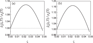
Figure 3: The average superfluid density as a function of the nematic-order state strength at (a) $\delta=0.15$ and (b) $\delta=0.12$ with $T=0.025J$. $\rho_{\rm s}(T)$ is the superfluid density in the case of the absence of the electronic nematicity.

To show the exotic behavior of the nematic-order state strength dependence of the average superfluid density $\bar{\rho}_{\rm s}(\varsigma,T)$ more clearly, we plot $\bar{\rho}_{\rm s}(\varsigma,T)$ as a function of the nematic-order state strength at (a) $\delta=0.15$ and (b) $\delta=0.12$ with $T=0.025J$ in Fig. 3. One can immediately see from the results in Fig. 3 that $\bar{\rho}_{\rm s}(\varsigma,T)$ presents a dome-like shape nematic-order state strength dependence, where a distinct peak appears at around the critical strength of the electronic nematicity $\varsigma_{\rm critical}\approx 0.023$, and then when the strength of the electronic nematicity is tuned away from the critical strength, this pronounced peak is suppressed at the lower strength as well as at the higher strength sides. More importantly, the strength range together with the critical strength of $\bar{\rho}_{\rm s}(\varsigma,T)$ at the underdoping $\delta=0.12$ are the exact same with those at the optimal doping $\delta=0.15$, indicating that the dome-like shape of the nematic-order state strength dependence of $\bar{\rho}_{\rm s}(\varsigma,T)$ occurs at a any given doping of the SC dome. This in turn leads to the enhancement of superconductivity Cao22 ; Cao21 , and gives rise to the dome-like shape of the nematic-order state strength dependence of $T_{\rm c}$. However, in the extremely high strength region $\varsigma>0.045$, $\bar{\rho}_{\rm s}(\varsigma,T)$ is less than that in the case of the absence of the electronic nematicity Liu20 , which leads to a reduction of $T_{\rm c}$.
(iii) The region at the temperature $T=T_{\rm c}$, where the SC gap $\bar{\Delta}^{(\varsigma)}({\bf k})|_{T=T_{\rm c}}=0$. Following our previous discussions in the case of the absence of the electronic nematicity Liu20 , the paramagnetic part of the response kernel in Eq. (27) can be reduced as,

$$K_{\hat{x}\hat{x}}^{({\rm p})}(\varsigma,{\bf q}\rightarrow 0,0)|_{T=T_{\rm c}} = -K_{\hat{x}\hat{x}}^{({\rm d})}(\varsigma,{\bf q}\rightarrow 0,0)|_{T=T_{\rm c}}$$ (32a)

$$= -{1\over\mu_{0}\lambda^{2}_{La}(\varsigma,T)}|_{T=T_{\rm c}},$$

$$K_{\hat{y}\hat{y}}^{({\rm p})}(\varsigma,{\bf q}\rightarrow 0,0)|_{T=T_{\rm c}} = -K_{\hat{y}\hat{y}}^{({\rm d})}(\varsigma,{\bf q}\rightarrow 0,0)|_{T=T_{\rm c}}$$ (32b)

$$= -{1\over\mu_{0}\lambda^{2}_{Lb}(\varsigma,T)}|_{T=T_{\rm c}},~{}~{}~{}~{}~{}~{}~{}$$

which exactly cancel the corresponding diamagnetic part of the response kernel in Eqs. (13a) and (13b), respectively, reflecting a basic fact that the Meissner effect in cuprate superconductors with coexisting electronic nematicity occurs below $T_{\rm c}$ only.

In summary, we have found the following results within the kinetic-energy-driven superconductivity: (i) the Meissner effect in cuprate superconductors with coexisting electronic nematicity is obtained for all temperature $T\leq T_{c}$; (ii) the electromagnetic response is inequivalent along with the $\hat{a}$- and $\hat{b}$-axes; (iii) the response kernels along the $\hat{a}$- and $\hat{b}$-axes are not manifestly gauge invariant within the bare current vertex in Eq. (22), however, the gauge invariance can be kept within the dressed current vertex Feng15 .

III.2 Local magnetic-field profile with broken rotation symmetry

We now turn to derive the local magnetic-field profile based on the standard specular reflection model with a two-dimensional geometry Abrikosov88 ; Tinkham96 . The local magnetic-field profile can be measured experimentally, e.g., by using the muon-spin rotation technique Jackson00 ; Khasanov04 ; Suter04 , reflecting the electromagnetic response and yielding the crucial information of the magnetic-field screening inside the sample. In cuprate superconductors, the experimental observations indicates an exponential character of the magnetic-field screening Jackson00 ; Khasanov04 ; Suter04 , in support of a local nature of the electrodynamics Schrieffer64 . However, the rotation symmetry-breaking of the response kernel (26) is inequivalent along the $\hat{a}$- and $\hat{b}$-axes. In this case, if the external magnetic-field is perpendicular to the ab plane, we can choose $A_{y}(x)$ along the $\hat{b}$-axis, or $A_{x}(y)$ along the $\hat{a}$-axis. From the following Maxwell equation,

$${\rm rot}\,{\bf B}={\rm rot}\,{\rm rot}\,{\bf A}={\rm grad}\,{\rm div}\,{\bf A}-\nabla^{2}\,{\bf A}=\mu_{0}{\bf J},$$ (33)

it can be found that the extension of the vector potential in an even manner through the boundary implies a kink in the $A_{y}(x)$ $[A_{x}(y)]$ curve. In other words, if the external magnetic field ${\bf B}$ is given at the system surface, i.e., $({\rm d}A_{y}(x)/{\rm d}x)|_{x=+0}=B$, while $({\rm d}A_{y}(x)/{\rm d}x)|_{x=-0}=-B$, or $({\rm d}A_{x}(y)/{\rm d}y)|_{y=+0}=B$, while $({\rm d}A_{x}(y)/{\rm d}y)|_{y=-0}=-B$, which Abrikosov88 indicates that the second derivative $({\rm d}^{2}A_{y}(x)/{\rm d}^{2}x)$ acquires a correction $2B\delta(x)$, or $({\rm d}^{2}A_{x}(y)/{\rm d}^{2}y)$ acquires a correction $2B\delta(y)$,

$${{\rm d}^{2}A_{y}(x)\over{\rm d}^{2}x}=2B\delta(x)-\mu_{0}J^{(\varsigma)}_{y},$$ (34a)

$${{\rm d}^{2}A_{x}(y)\over{\rm d}^{2}y}=2B\delta(y)-\mu_{0}J^{(\varsigma)}_{x},$$ (34b)

where the transverse gauge ${\rm div}\,{\bf A}=0$ has been adopted. In the momentum space, the above these equations can be expressed as,

$$q_{x}^{2}A_{y}({\bf q})=\mu_{0}J^{(\varsigma)}_{y}({\bf q})-2B,$$ (35a)

$$q_{y}^{2}A_{x}({\bf q})=\mu_{0}J^{(\varsigma)}_{x}({\bf q})-2B.$$ (35b)

Substituting this Fourier transform form (35) into Eq. (8), and performing a solution for the vector potential, the relations between the vector potential and the response kernels can be obtained as,

$$A_{y}({\bf q})=-2B{\delta(q_{y})\delta(q_{z})\over\mu_{0}K_{\hat{y}\hat{y}}(\varsigma,{\bf q})+q_{x}^{2}},$$ (36a)

$$A_{x}({\bf q})=-2B{\delta(q_{x})\delta(q_{z})\over\mu_{0}K_{\hat{x}\hat{x}}(\varsigma,{\bf q})+q_{y}^{2}}.$$ (36b)

Since the vector potential has only the $\hat{y}$ [$\hat{x}$] component, the non-zero component of the local magnetic-field ${\bf h}=\rm{rot}\,{\bf A}$ is that along the $z$ axis as $h^{(\varsigma)}_{zx}({\bf q})=iq_{x}A_{y}({\bf q})$ [$h^{(\varsigma)}_{zy}({\bf q})=iq_{y}A_{x}({\bf q})$].

With the help of the above relations in Eq. (36) and the response kernels in Eq. (29), the local magnetic-field profiles along the $\hat{a}$- and $\hat{b}$-axes in the long wavelength limit can be derived straightforwardly as,

$$h^{(\varsigma)}_{z}(x) = {B\over\pi}\int\limits_{-\infty}^{\infty}{\rm{d}}q_{x}\,{q_{x}\sin(q_{x}x)\over\mu_{0}K_{\hat{y}\hat{y}}(\varsigma,q_{x}\rightarrow 0,0,0)+q_{x}^{2}}$$ (37a)

$$= 2Be^{-{x\over\lambda_{b}(\varsigma,T)}},~{}~{}~{}~{}$$

$$h^{(\varsigma)}_{z}(y) = {B\over\pi}\int\limits_{-\infty}^{\infty}{\rm{d}}q_{y}\,{q_{y}\sin(q_{y}y)\over\mu_{0}K_{\hat{x}\hat{x}}(\varsigma,q_{y}\rightarrow 0,0,0)+q_{y}^{2}}$$ (37b)

$$= 2Be^{-{y\over\lambda_{a}(\varsigma,T)}},~{}~{}~{}~{}$$

respectively. In a striking analogy to the case of the absence of the electronic nematicity Liu20 , the distance dependence of $h^{(\varsigma)}_{z}(x)$ [$h^{(\varsigma)}_{z}(y)$)] follows an exponential law as was expected for the local electrodynamic response. However, the magnitude of $h^{(\varsigma)}_{z}(x)$ along the $\hat{a}$-axis at a given distance is unequal to the corresponding one of $h^{(\varsigma)}_{z}(y)$ along the $\hat{b}$-axis, with the difference of the magnitudes between $h^{(\varsigma)}_{z}(x)$ and $h^{(\varsigma)}_{z}(y)$ that is increased with the increase of distance, in qualitative agreement with the experimental results Kiefl10 . This anisotropic feature therefore reflects an experimental fact that the electromagnetic response is inequivalent along the $\hat{a}$- and $\hat{b}$-axes Kiefl10 .

The enhancement of the superfluid density by the electronic nematicity can be attributed to the enhancement of the SC condensation energy, i.e., the energy of the system in the SC-state with coexisting nematic order is lower than the energy in the SC-state with the absence of the nematic order. In other words, the SC-state with coexisting nematic order is more stable than the SC-state with the absence of the nematic order. The internal energy $U^{\rm(s)}_{\varsigma}(T)$ of the system can be expressed as,

$$U^{\rm(s)}_{\varsigma}(T)=2\int\limits_{-\infty}^{\infty}{{\rm{d}}\omega\over 2\pi}\rho^{\rm(s)}(\omega,T,\varsigma)\omega n_{\rm F}(\omega),~{}~{}~{}~{}$$ (38)

with the fermion distribution function $n_{\rm F}(\omega)$, and the electron density of states $\rho^{\rm(s)}(\omega,T,\varsigma)$,

$$\rho^{\rm(s)}(\omega,T,\varsigma)={1\over N}\sum_{{\bf k}}A_{\varsigma}({\bf k},\omega,T),~{}~{}~{}$$ (39)

where the electron spectral function $A_{\varsigma}({\bf k},\omega,T)=-2{\rm Im}G^{\rm(RMF)}_{\varsigma}({\bf k},\omega)$ is obtained directly from the electron diagonal propagator $G^{\rm(RMF)}_{\varsigma}({\bf k},\omega)$ in Eq. (4) as,

$$A_{\varsigma}({\bf k},\omega,T) = \pi Z^{(\varsigma)}_{\rm F}\left[\left(1+{\bar{\varepsilon}^{(\varsigma)}_{\bf k}\over E^{(\varsigma)}_{\bf k}}\right)\delta(\omega-E^{(\varsigma)}_{\bf k})\right.$$ (40)

$$+ \left.\left(1-{\bar{\varepsilon}^{(\varsigma)}_{\bf k}\over E^{(\varsigma)}_{\bf k}}\right)\delta(\omega+E^{(\varsigma)}_{\bf k})\right].~{}~{}~{}$$

Substituting $A_{\varsigma}({\bf k},\omega,T)$ in Eq. (40) into Eqs. (39) and (38), $U^{\rm(s)}_{\varsigma}(T)$ can be evaluated as,

$$U^{(\rm s)}_{\varsigma}(T)=-{Z^{(\varsigma)}_{{\rm F}}\over N}\sum_{\bf k}[E^{(\varsigma)}_{\bf k}{\rm tanh}({1\over 2}\beta E^{(\varsigma)}_{\bf k}]+{Z^{(\varsigma)}_{{\rm F}}\over N}\sum_{\bf k}\bar{\varepsilon}^{(\varsigma)}_{\bf k}.~{}~{}~{}~{}~{}$$ (41)

In the normal-state, the SC gap $\bar{\Delta}^{(\varsigma)}({\bf k})=0$, this internal energy is reduced as,

$$U^{(\rm n)}_{\varsigma}(T)=-{Z^{(\varsigma)}_{{\rm F}}\over N}\sum_{\bf k}[\bar{\varepsilon}^{(\varsigma)}_{\bf k}{\rm tanh}({1\over 2}\beta\bar{\varepsilon}^{(\varsigma)}_{\bf k})]+{Z^{(\varsigma)}_{{\rm F}}\over N}\sum_{\bf k}\bar{\varepsilon}^{(\varsigma)}_{\bf k}.~{}~{}~{}~{}~{}$$ (42)

At zero temperature, the SC condensation energy $E^{({\varsigma})}_{\rm cond}(T)$ can be obtained as,

$$E^{(\varsigma)}_{\rm cond} = U^{(\rm n)}_{{\varsigma}}(T)-U^{(\rm s)}_{{\varsigma}}(T)|_{T=0}.~{}~{}~{}~{}~{}$$ (43)

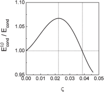
Figure 4: The superconducting condensation energy as a function of the nematic-order state strength at $\delta=0.15$. $E_{\rm cond}$ is the superconducting condensation energy in the case of the absence of the electronic nematicity.

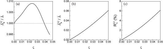
Figure 5: (a) The d-wave component of the superconducting gap parameter, (b) the s-wave component of the superconducting gap parameter, and (c) the ratio of the s-wave component to d-wave component as a function of the nematic-order state strength at $\delta=0.15$ with $T=0$. $\bar{\Delta}$ is the superconducting gap parameter in the case of the absence of the electronic nematicity.

In Fig. 4, we plot $E^{(\varsigma)}_{\rm cond}$ as a function of the nematic-order state strength at $\delta=0.15$, where there is the surprising similarity between the $E^{(\varsigma)}_{\rm cond}$ and $\bar{\rho}_{\rm s}(\varsigma)$ with the following characteristic features: (i) $E^{(\varsigma)}_{\rm cond}$ is enhanced by the electronic nematicity in the whole strength range of the electronic nematicity except for in the the extremely strong strength region $\varsigma>0.04$, where $E^{(\varsigma)}_{\rm cond}$ is reduced. This enhancement of $E^{(\varsigma)}_{\rm cond}$ therefore induces the enhancement of $\bar{\rho}_{\rm s}(\varsigma,T)$. The result in Fig. 4 also reflects a fact that the strong electron correlation induces the system to find new way to lower its ground-state energy by the spontaneous breaking of the native rotation symmetry of the square lattice underlying the copper-oxide plane Kivelson19 ; Vojta09 ; Fradkin10 ; Fernandes19 . In other words, as the appearance of superconductivity, the emergence of the electronic nematicity together with the associated fluctuation phenomena in the whole strength range of the electronic nematicity except for in the extremely strong strength region are a natural consequence of the strong electron correlation effect; (ii) However, there is a substantial difference, namely, $E^{(\varsigma)}_{\rm cond}$ less than that in the case of the absence of the electronic nematicity occurs at the extremely strong strength region $\varsigma>0.04$, rather than at the extremely high strength region $\varsigma>0.045$, where $\bar{\rho}_{\rm s}(\varsigma,T)$ is less than that in the case of the absence of the electronic nematicity, although the crossover strength $\varsigma_{\rm essr}=0.04$ in $E^{(\varsigma)}_{\rm cond}$ is not far from the crossover strength $\varsigma_{\rm ehsr}=0.045$ in $\bar{\rho}_{\rm s}(\varsigma,T)$. However, the actual weak strength region of the order of the magnitude of the strength $\varsigma$ with the high impacts on various properties Nakata18 ; Sato17 ; Daou10 is exactly same in $E^{(\varsigma)}_{\rm cond}$ and $\bar{\rho}_{\rm s}(\varsigma,T)$. Moreover, the optimal strength $\varsigma_{\rm optimal}\approx 0.022$ for the maximal $E^{(\varsigma)}_{\rm cond}$ is quite close to the critical strength $\varsigma_{\rm critical}\approx 0.023$ for the highest $\bar{\rho}_{\rm s}(\varsigma,T)$.

We now turn to show (i) why $E^{({\varsigma})}_{\rm cond}$ has a dome-like shape of the nematic-order state strength dependence? and (ii) why $E^{({\varsigma})}_{\rm cond}$ is reduced by the electronic nematicity in the extremely strong strength region? The expression form of the SC condensation energy in Eq. (43) also indicates that $E^{({\varsigma})}_{\rm cond}$ is proportional to the SC gap, i.e., $E^{({\varsigma})}_{\rm cond}(T)\propto\bar{\Delta}^{(\varsigma)}$. The SC gap measures the strength of the binding of electrons into electron pairs Schrieffer64 ; Bonn96 ; Sonier00 ; Basov05 ; Sonier16 , while the superfluid density is a measure of the phase stiffness Schrieffer64 ; Bonn96 ; Sonier00 ; Basov05 ; Sonier16 , therefore the SC gap and superfluid density separately describe the different aspects of the same SC quasiparticles. In the case of the absence of the electronic nematicity Feng15a , the pure d-wave electron pairs with the electron pair strength $\bar{\Delta}\gamma^{\rm(d)}_{\bf k}$ condensation reveals the SC-state with the pure d-wave symmetry. However, the present result of Eq. (7) in the SC-state with coexisting nematic order shows that in addition to the pure d-wave component of the SC gap $\bar{\Delta}^{(\varsigma)}_{\rm d}\gamma^{\rm(d)}_{\bf k}$, the pure s-wave component of the SC gap $\bar{\Delta}^{(\varsigma)}_{\rm s}\gamma^{\rm(s)}_{\bf k}$ is induced by the electronically nematic order, therefore there is a coexistence and competition between the d-wave component of the SC gap parameter $\bar{\Delta}^{(\varsigma)}_{\rm d}$ and the s-wave component of the SC gap parameter $\bar{\Delta}^{(\varsigma)}_{\rm s}$. This coexistence and competition is closely related to the strength of the electronic nematicity, and therefore plays a crucial role in the exotic features of the nematic-order state strength dependence of the electromagnetic response. To show this point more clearly, we plot (a) the d-wave component of the SC gap parameter $\bar{\Delta}^{(\varsigma)}_{\rm d}$, (b) the s-wave component of the SC gap parameter $\bar{\Delta}^{(\varsigma)}_{\rm s}$, and (c) the ratio of the s-wave component to d-wave component $R^{(\varsigma)}_{\Delta}=\bar{\Delta}^{(\varsigma)}_{\rm s}/\bar{\Delta}^{(\varsigma)}_{\rm d}$ as a function of the nematic-order state strength at $\delta=0.15$ with $T=0$ in Fig. 5, where the key features can be summarized as: (i) $\bar{\Delta}^{(\varsigma)}_{\rm d}$ exhibits a dome-like shape nematic-order state strength dependence (see Fig. 5a), while the result shows a almost linear characteristics of $\bar{\Delta}^{(\varsigma)}_{\rm s}$ (see Fig. 5b). In other words, $\bar{\Delta}^{(\varsigma)}_{\rm s}$ increases monotonically with the increase of the nematic-order state strength in the whole strength range of the electronic nematicity, while $\bar{\Delta}^{(\varsigma)}_{\rm d}$ is enhanced by the electronic nematicity from the weak to strong strength regions of the electronic nematicity except for in the the extremely strong strength region, where $\bar{\Delta}^{(\varsigma)}_{\rm d}$ is reduced. In particular, the nematic-order state strength range of the SC dome together with the optimal strength in $\bar{\Delta}^{(\varsigma)}_{\rm d}$ are almost the same with those in $\bar{\rho}_{\rm s}(\varsigma,T)$, which is an evidence that the nematic-order state strength dependence of $\bar{\rho}_{\rm s}(\varsigma,T)$ is mainly determined by the nematic-order state strength dependence of $\bar{\Delta}^{(\varsigma)}_{\rm d}$; (ii) In the lower ratio region ($0<R^{(\varsigma)}_{\Delta}<2.29\%$, see Fig. 5c), which is corresponding to the weak strength region of the electronic nematicity ($\varsigma<0.022$), the electronic nematicity induces an increase of both $\bar{\Delta}^{(\varsigma)}_{\rm d}$ and $\bar{\Delta}^{(\varsigma)}_{\rm s}$. In particular, although the increase rate for $\bar{\Delta}^{(\varsigma)}_{\rm d}$ is slower than that in $\bar{\Delta}^{(\varsigma)}_{\rm s}$, the maximal SC gap parameter $\bar{\Delta}^{(\varsigma)}$ in Eq. (7) is increased, which leads to that $\bar{\rho}_{\rm s}(\varsigma,T)$ increase with the increase of the nematic-order state strength in the lower ratio region. However, in the higher ratio region ($4.66\%>R^{(\varsigma)}_{\Delta}>2.29\%$), which is corresponding to the strong strength region of the electronic nematicity ($0.022<\varsigma<0.04$), the electronic nematicity tends to support the high speed increase of $\bar{\Delta}^{(\varsigma)}_{\rm s}$, concomitantly, $\bar{\Delta}^{(\varsigma)}_{\rm d}$ is decreased. In this case, the maximal SC gap parameter $\bar{\Delta}^{(\varsigma)}$ in Eq. (7) is decreased, which leads to that $\bar{\rho}_{\rm s}(\varsigma,T)$ decrease with the increase of the nematic-order state strength in the higher ratio region. The optimal ratio region ($R^{(\varsigma)}_{\Delta}\sim 2.29\%$), corresponding to the optimal strength of the electronic nematicity ($\varsigma=0.022$), is a balance region, where both $\bar{\Delta}^{(\varsigma)}_{\rm d}$ and $\bar{\Delta}^{(\varsigma)}_{\rm s}$ and the nematic-order state strength are optimally matched, leading to that the highest $\bar{\rho}_{\rm s}(\varsigma,T)$ appears at around the optimal ratio region. This is why the highest $\bar{\rho}_{\rm s}(\varsigma,T)$ occurs at around the optimal ratio region, and then decreases in both the lower and higher ratio regions. However, in the extremely higher ratio region ($R^{(\varsigma)}_{\Delta}>4.66\%$), which is corresponding to the extremely strong strength region of the electronic nematicity, the increased part in $\bar{\Delta}^{(\varsigma)}_{\rm s}$ can not compensate for the lost part in $\bar{\Delta}^{(\varsigma)}_{\rm d}$, and then the maximal SC gap parameter $\bar{\Delta}^{(\varsigma)}$ in Eq. (7) is less than that in the case of the absence of the electronic nematicity, which leads to that $\bar{\rho}_{\rm s}(\varsigma,T)$ is less than that in the case of the absence of the electronic nematicity. This is why $\bar{\rho}_{\rm s}(\varsigma,T)$ in the extremely strong strength region is lower than that in the case of the absence of the electronic nematicity.

IV Summary and discussion

Within the framework of the kinetic-energy-driven superconductivity, we have investigated the nematic-order state strength dependence of the electromagnetic response in cuprate superconductors in terms of the linear response approach, where the rotation symmetry-breaking of the response kernel is evaluated and employed to calculate the magnetic-field penetration-depth, the superfluid density, and the local magnetic-field profile, for a purely transverse vector potential. Our results indicate that the electromagnetic response of cuprate superconductors with coexisting electronic nematicity is inequivalent along the $\hat{a}$- and $\hat{b}$-axes. In particular, the calculated local-magnetic-field profiles along the $\hat{a}$- and $\hat{b}$-axes as a function of distance and the magnetic-field penetration-depths along the $\hat{a}$- and $\hat{b}$-axes for the optimal strength of the electronic nematicity are qualitatively consistent with the corresponding experimental results Kiefl10 ; Quijada99 . The obtained results also show that in addition to the pure d-wave component of the SC gap, the pure s-wave component of the SC gap is generated by the electronically nematic order, therefore there is a coexistence and competition of the pure d-wave component and the pure s-wave component. However, this coexistence and competition leads to the average superfluid density that first increases with the strength of the electronic nematicity in the lower strength region, then reaches a maximum value at around the critical strength of the electronic nematicity, but is suppressed with further increase of the strength in the higher strength region of the electronic nematicity, which in turn induces the enhancement of superconductivity, and gives rise to the dome-like shape of the nematic-order state strength dependence of the superfluid density.

Finally, it should be emphasized that besides the emergence of the electronic nematicity in cuprate superconductors Fradkin15 ; Kivelson19 ; Vojta09 ; Fradkin10 ; Fernandes19 , the electronically nematic order has been detected from other families of the unconventional superconductors, including the iron-based superconductors Chuang10 ; Gallais13 ; Massat16 ; Baek20 , the strontium ruthenate superconductors Borzi07 , as well as the nickel-based superconductors Eckberg20 , and then a characteristic feature in the complicated phase diagrams of these unconventional superconductors is the interplay between the electronic nematicity and superconductivity. In this case, the theoretical framework developed in this paper for the understanding of the nature of the electromagnetic response of cuprate superconductors with coexisting electronic nematicity can be also employed to study the electromagnetic response of these unconventional superconductors with coexisting electronic nematicity Chuang10 ; Gallais13 ; Massat16 ; Baek20 ; Borzi07 ; Eckberg20 . In particular, in the iron-based superconductors Chuang10 ; Gallais13 ; Massat16 ; Baek20 , the SC gap with a simple $s_{\pm}$ symmetry $|\Delta({\bf k})|=|\Delta_{0}\gamma^{\rm(s)}_{\bf k}|=\Delta_{0}|\cos k_{x}+\cos k_{y}|/2$ in the case of the absence of the electronic nematicity is modified as,

$$|\Delta^{(\varsigma)}_{0}({\bf k})|=|\Delta^{(\varsigma)}_{\rm 0s}\gamma^{\rm(s)}_{\bf k}+\Delta^{(\varsigma)}_{\rm 0d}\gamma^{\rm(d)}_{\bf k}|,$$ (44)

in the case of the presence of the electronic nematicity, where $\Delta^{(\varsigma)}_{\rm 0s}=(\Delta^{(\varsigma)}_{0\hat{x}}+\Delta^{(\varsigma)}_{0\hat{y}})/2$ and $\Delta^{(\varsigma)}_{\rm 0d}=(\Delta^{(\varsigma)}_{0\hat{x}}-\Delta^{(\varsigma)}_{0\hat{y}})/2$ are the s-wave and d-wave components of the SC gap parameter, respectively. It thus shows that this modification in Eq. (44) arising from the emergence of the electronic nematicity in the iron-based superconductors Chuang10 ; Gallais13 ; Massat16 ; Baek20 induces a deviation from the pure $s_{\pm}$ pairing symmetry.

Disclosure statement

No potential conflict of interest was reported by the authors.

Funding

ZC, XM, and SF are supported by the National Key Research and Development Program of China under Grant No. 2021YFA1401803, and the National Natural Science Foundation of China (NSFC) under Grant Nos. 11974051 and 12274036. HG is supported by NSFC under Grant Nos. 11774019 and 12074022, and the Fundamental Research Funds for the Central Universities and HPC resources at Beihang University.

Appendix A Electron propagator

This Appendix presents the derivation of the vertex corrected electron propagator $\mathbb{G}_{\varsigma}({\bf k},\omega)$ in Eq. (4) of the main text. In the fermion-spin representation (3), the original $t$-$J$ model in Eq. (1) at zero magnetic field can be rewritten as,

$$H = \sum_{l\hat{\eta}}t_{\hat{\eta}}(h^{\dagger}_{l+\hat{\eta}\uparrow}h_{l\uparrow}S^{+}_{l}S^{-}_{l+\hat{\eta}}+h^{\dagger}_{l+\hat{\eta}\downarrow}h_{l\downarrow}S^{-}_{l}S^{+}_{l+\hat{\eta}})$$ (45)

$$- \sum_{l\hat{\eta}^{\prime}}t^{\prime}_{\hat{\eta}^{\prime}}(h^{\dagger}_{l+\hat{\eta}^{\prime}\uparrow}h_{l\uparrow}S^{+}_{l}S^{-}_{l+\hat{\eta}^{\prime}}+h^{\dagger}_{l+\hat{\eta}^{\prime}\downarrow}h_{l\downarrow}S^{-}_{l}S^{+}_{l+\hat{\eta}^{\prime}})$$

$$- \mu_{\rm h}\sum_{l\sigma}h^{\dagger}_{l\sigma}h_{l\sigma}+\sum_{l\hat{\eta}}J^{(\hat{\eta})}_{\rm eff}{\bf S}_{l}\cdot{\bf S}_{l+\hat{\eta}},~{}~{}~{}~{}~{}~{}$$

where $\mu_{\rm h}$ is the charge-carrier chemical potential, $S^{-}_{l}$ and $S^{+}_{l}$ are the spin-lowering and spin-raising operators for the spin $S=1/2$, respectively, $J_{\rm eff}^{(\hat{\eta})}=(1-\delta)^{2}J_{\hat{\eta}}$ is the effective exchange coupling, and $\delta=\langle h^{\dagger}_{l\sigma}h_{l\sigma}\rangle$ is the doping concentration.

Within the framework of the kinetic-energy driven superconductivity Feng15 ; Feng0306 ; Feng12 , it has been shown that the interaction between the charge carriers directly from the kinetic energy of the $t$-$J$ model (45) by the exchange of a strongly dispersive spin excitation generates the charge-carrier pairing state with coexisting nematic order Cao22 ; Cao21 , where the charge-carrier diagonal and off-diagonal propagators satisfy the following self-consistent equations as,

$$g_{\varsigma}({\bf k},\omega) = g^{(0)}_{\varsigma}({\bf k},\omega)+g^{(0)}_{\varsigma}({\bf k},\omega)[\Sigma^{(\rm h)}_{{\rm ph}}(\varsigma,{\bf k},\omega)g_{\varsigma}({\bf k},\omega)$$ (46a)

$$- \Sigma^{(\rm h)}_{{\rm pp}}(\varsigma,{\bf k},\omega)\Gamma^{\dagger}_{\varsigma}({\bf k},\omega)],~{}~{}~{}~{}~{}~{}~{}$$

$$\Gamma^{\dagger}_{\varsigma}({\bf k},\omega) = g^{(0)}_{\varsigma}({\bf k},-\omega)[\Sigma^{(\rm h)}_{{\rm ph}}(\varsigma,{\bf k},-\omega)\Gamma^{\dagger}_{\varsigma}({\bf k},\omega)$$ (46b)

$$+ \Sigma^{(\rm h)}_{{\rm pp}}(\varsigma,{\bf k},\omega)g_{\varsigma}({\bf k},\omega)],~{}~{}~{}~{}$$

where $g^{(0)}_{\varsigma}({\bf k},\omega)$ is the mean-field (MF) charge-carrier diagonal propagator, and has been given explicitly in Ref. Cao22, , while $\Sigma^{(\rm h)}_{\rm ph}(\varsigma,{\bf k},\omega)$ and $\Sigma^{(\rm h)}_{\rm pp}(\varsigma,{\bf k},\omega)$ are the charge-carrier self-energies in the particle-hole and particle-particle channels, respectively, and have been obtained in terms of the spin bubble as Cao22 ; Cao21 ,

$$\Sigma^{({\rm h})}_{{\rm ph}}(\varsigma,{\bf k},i\omega_{n}) = {1\over N^{2}}\sum_{{\bf p},{\bf p}^{\prime}}[\Lambda^{(\varsigma)}_{{\bf p}+{\bf p}^{\prime}+{\bf k}}]^{2}$$

$$\times {1\over\beta}\sum_{ip_{m}}g_{\varsigma}({{\bf p}+{\bf k}},ip_{m}+i\omega_{n})\Pi_{\varsigma}({\bf p},{\bf p}^{\prime},ip_{m}),$$

(47a)

$$\Sigma^{({\rm h})}_{{\rm pp}}(\varsigma,{\bf k},i\omega_{n}) = {1\over N^{2}}\sum_{{\bf p},{\bf p}^{\prime}}[\Lambda^{(\varsigma)}_{{\bf p}+{\bf p}^{\prime}+{\bf k}}]^{2}$$

$$\times {1\over\beta}\sum_{ip_{m}}\Gamma^{\dagger}_{\varsigma}({\bf p}+{\bf k},ip_{m}+i\omega_{n})\Pi_{\varsigma}({\bf p},{\bf p}^{\prime},ip_{m}),$$

with the fermionic and bosonic Matsubara frequencies $\omega_{n}$ and $p_{m}$, respectively, the bare vertex function $\Lambda^{(\varsigma)}_{\bf k}=4t[(1-\varsigma)\gamma_{{\bf k}_{x}}+(1+\varsigma)\gamma_{{\bf k}_{y}}]-4t^{\prime}\gamma_{\bf{k}}^{\prime}$, and the spin bubble,

$$\Pi_{\varsigma}({\bf p},{\bf p}^{\prime},ip_{m}) = {1\over\beta}\sum_{ip_{m}^{\prime}}D^{(0)}_{\varsigma}({\bf p}^{\prime},ip_{m}^{\prime})$$ (48)

$$\times D^{(0)}_{\varsigma}({\bf p^{\prime}+p},ip_{m}^{\prime}+ip_{m}),$$

where the MF spin propagator $D^{(0)}_{\varsigma}({\bf k},\omega)$ in the presence of the electronic nematicity has been derived as Cao22 ,

$$D^{(0)}_{\varsigma}({\bf k},\omega) = {B^{(\varsigma)}_{\bf k}\over 2\omega^{(\varsigma)}_{\bf k}}\left({1\over\omega-\omega^{(\varsigma)}_{\bf k}}-{1\over\omega+\omega^{(\varsigma)}_{\bf k}}\right),$$ (49)

with the spin orthorhombic excitation spectrum $\omega^{(\varsigma)}_{\bf k}$, and the weight function of the spin excitation spectrum $B^{(\varsigma)}_{{\bf{k}}}$ that have been given explicitly in Ref. Cao22, .

For the derivation of the electron diagonal and off-diagonal propagators, a full charge-spin recombination scheme has been proposed based on the kinetic-energy-driven superconductivity Feng15a , where the coupling form between the electrons and a strongly dispersive spin excitation is the same as that between the charge carriers and a strongly dispersive spin excitation, i.e., the form of the self-consistent equations fulfilled by the electron diagonal and off-diagonal propagators is the same as the form in Eq. (46) fulfilled by the charge-carrier diagonal and off-diagonal propagators. In this case, a charge carrier and a localized spin in the fermion-spin representation (3) are fully recombined into a constrained electron in which the charge-carrier diagonal and off-diagonal propagators $g_{\varsigma}({\bf k},\omega)$ and $\Gamma^{\dagger}_{\varsigma}({\bf k},\omega)$ in Eq. (46) are replaced by the electron diagonal and off-diagonal propagators $G_{\varsigma}({\bf k},\omega)$ and $\Im^{\dagger}_{\varsigma}({\bf k},\omega)$, respectively, and then the electron diagonal and off-diagonal propagators of the $t$-$J$ model (1) at zero magnetic field satisfy the following self-consistent equations,

$$G_{\varsigma}({\bf k},\omega) = G^{(0)}_{\varsigma}({\bf k},\omega)+G^{(0)}_{\varsigma}({\bf k},\omega)[\Sigma^{(\varsigma)}_{\rm ph}({\bf k},\omega)G_{\varsigma}({\bf k},\omega)$$ (50a)

$$- \Sigma^{(\varsigma)}_{\rm pp}({\bf k},\omega)\Im^{\dagger}_{\varsigma}({\bf k},\omega)],~{}~{}~{}~{}~{}~{}~{}$$

$$\Im^{\dagger}_{\varsigma}({\bf k},\omega) = G^{(0)}_{\varsigma}({\bf k},-\omega)[\Sigma^{(\varsigma)}_{\rm ph}({\bf k},-\omega)\Im^{\dagger}_{\varsigma}({\bf k},\omega)$$ (50b)

$$+ \Sigma^{(\varsigma)}_{\rm pp}({\bf k},\omega)G_{\varsigma}({\bf k},\omega)],~{}~{}~{}~{}~{}~{}$$

where $G^{(0)}_{\varsigma}({\bf k},\omega)$ is the electron diagonal propagator of the $t$-$J$ model (1) at zero magnetic field in the tight-binding approximation, and has been obtained as Cao22 ,

$$G^{(0)}_{\varsigma}({\bf k},\omega) = {1\over\omega-\varepsilon^{(\varsigma)}_{\bf k}},$$ (51)

while the electron self-energies $\Sigma^{(\varsigma)}_{\rm ph}({\bf k},\omega)$ in the particle-hole channel and $\Sigma^{(\varsigma)}_{\rm pp}({\bf k},\omega)$ in the particle-particle channel can be obtained directly from the corresponding parts of the charge-carrier self-energies $\Sigma^{(\rm h)}_{{\rm ph}}(\varsigma,{\bf k},\omega)$ in the particle-hole channel and $\Sigma^{(\rm h)}_{{\rm pp}}(\varsigma,{\bf k},\omega)$ in the particle-particle channel in Eq. (47) by the replacement of the full charge-carrier diagonal and off-diagonal propagators $g_{\varsigma}({\bf k},\omega)$ and $\Gamma^{\dagger}_{\varsigma}({\bf k},\omega)$ with the corresponding full electron diagonal and off-diagonal propagators $G_{\varsigma}({\bf k},\omega)$ and $\Im^{\dagger}_{\varsigma}({\bf k},\omega)$ as,

$$\Sigma^{(\varsigma)}_{\rm ph}({\bf k},i\omega_{n}) = {1\over N^{2}}\sum_{{\bf p},{\bf p}^{\prime}}[\bar{\Lambda}^{(\varsigma)}_{{\bf p}+{\bf p}^{\prime}+{\bf k}}]^{2}$$

$$\times {1\over\beta}\sum_{ip_{m}}G_{\varsigma}({{\bf p}+{\bf k}},ip_{m}+i\omega_{n})\Pi_{\varsigma}({\bf p},{\bf p}^{\prime},ip_{m}),$$

(52a)

$$\Sigma^{(\varsigma)}_{\rm pp}({\bf k},i\omega_{n}) = {1\over N^{2}}\sum_{{\bf p},{\bf p}^{\prime}}[\bar{\Lambda}^{(\varsigma)}_{{\bf p}+{\bf p}^{\prime}+{\bf k}}]^{2}$$

$$\times {1\over\beta}\sum_{ip_{m}}\Im^{\dagger}_{\varsigma}({\bf p}+{\bf k},ip_{m}+i\omega_{n})\Pi_{\varsigma}({\bf p},{\bf p}^{\prime},ip_{m}),$$

with the vertex function $\bar{\Lambda}^{(\varsigma)}_{\bf k}=4t[V^{(x)}_{\rm cor}(1-\varsigma)\gamma_{{\bf k}_{x}}+V^{(y)}_{\rm cor}(1+\varsigma)\gamma_{{\bf k}_{y}}]-2t^{\prime}(V^{(x)}_{\rm cor}+V^{(y)}_{\rm cor})\gamma_{\bf{k}}^{\prime}$, where the vertex correct in terms of $V^{(x)}_{\rm cor}$ and $V^{(y)}_{\rm cor}$ for the electron self-energies in the particle-hole and particle-particle channels has been introduced for a better description of the nematic-order state strength dependence of the electromagnetic response, which is different from the previous discussions of the electronic structure of cuprate superconductors with coexisting electronic nematicity Cao22 ; Cao21 , where this vertex correct is ignored. As in the previous discussions Cao22 ; Cao21 , the electron self-energy in the particle-hole channel $\Sigma^{(\varsigma)}_{\rm ph}({\bf k},\omega)$ represents the electron quasiparticle coherence, while the electron self-energy in the particle-particle channel $\Sigma^{(\varsigma)}_{\rm pp}({\bf k},\omega)$ represents the momentum and energy dependence of the SC gap, $\Sigma^{(\varsigma)}_{\rm pp}({\bf k},\omega)=\bar{\Delta}^{(\varsigma)}({\bf k},\omega)$.

In order to self-consistently determine all the parameters, the next step is to separate the electron self-energy $\Sigma^{(\varsigma)}_{\rm ph}({\bf k},\omega)$ in the particle-hole channel into its symmetric and antisymmetric parts as: $\Sigma^{(\varsigma)}_{\rm ph}({\bf k},\omega)=\Sigma^{(\varsigma)}_{\rm phe}({\bf k},\omega)+\omega\Sigma^{(\varsigma)}_{\rm pho}({\bf k},\omega)$. Following the common practice, this antisymmetric part $\Sigma^{(\varsigma)}_{\rm pho}({\bf k},\omega)$ is defined as the electron quasiparticle coherent weight: $Z^{(\varsigma)-1}_{\rm F}({\bf k},\omega)=1-{\rm Re}\Sigma^{(\varsigma)}_{\rm pho}({\bf k},\omega)$. In an interacting electron system, everything happens near the electron Fermi surface (EFS). As a case in low-energy close to EFS, the SC gap and electron quasiparticle coherent weight can be discussed in the static-limit approximation,

$$\bar{\Delta}^{(\varsigma)}({\bf k}) = \bar{\Delta}^{(\varsigma)}_{\hat{x}}\gamma_{{\bf k}_{x}}-\bar{\Delta}^{(\varsigma)}_{\hat{y}}\gamma_{{\bf k}_{y}},$$ (53a)

$${1\over Z^{(\varsigma)}_{\rm F}} = 1-{\rm Re}\Sigma^{(\varsigma)}_{\rm pho}({\bf k},\omega=0)\mid_{{\bf k}=[\pi,0]},~{}~{}~{}$$ (53b)

where the wave vector ${\bf k}$ in $Z^{(\varsigma)}_{\rm F}({\bf k})$ has been chosen as ${\bf k}=[\pi,0]$ just as it has been done in the ARPES experiments DLFeng00 ; Ding01 .

With the help of the above static-limit approximation for $\bar{\Delta}^{(\varsigma)}({\bf k})$ and $Z^{(\varsigma)}_{\rm F}$ in Eq. (53), the renormalized electron diagonal and off-diagonal propagators are obtained from Eq. (50) as,

$$G^{\rm(RMF)}_{\varsigma}({\bf k},\omega) = Z^{(\varsigma)}_{\rm F}\left({U^{(\varsigma)2}_{\bf k}\over\omega-E^{(\varsigma)}_{\bf k}}+{V^{(\varsigma)2}_{\bf k}\over\omega+E^{(\varsigma)}_{\bf k}}\right),$$ (54a)

$$\Im^{{\rm(RMF)}\dagger}_{\varsigma}({\bf k},\omega) = -Z^{(\varsigma)}_{\rm F}{\bar{\Delta}^{(\varsigma)}_{\rm Z}({\bf k})\over 2E^{(\varsigma)}_{\bf k}}\left({1\over\omega-E^{(\varsigma)}_{\bf k}}-{1\over\omega+E^{(\varsigma)}_{\bf k}}\right),$$

where the SC quasiparticle coherence factors $U^{(\varsigma)}_{\bf k}$ and $V^{(\varsigma)}_{\bf k}$ are given explicitly by,

$$U^{(\varsigma)2}_{\bf k} = {1\over 2}\left(1+{\bar{\varepsilon}^{(\varsigma)}_{\bf k}\over E^{(\varsigma)}_{\bf k}}\right),$$ (55a)

$$V^{(\varsigma)2}_{\bf k} = {1\over 2}\left(1-{\bar{\varepsilon}^{(\varsigma)}_{\bf k}\over E^{(\varsigma)}_{\bf k}}\right),$$ (55b)

and fulfills the constraint $U^{(\varsigma)2}_{\bf k}+V^{(\varsigma)2}_{\bf k}=1$. In particular, the renormalized electron diagonal and off-diagonal propagators in Eq. (54) can be also expressed explicitly in the Nambu representation as quoted in Eq. (4).

Substituting these renormalized electron diagonal and off-diagonal propagators in Eq. (54) and MF spin propagator in Eq. (49) into Eqs. (52) and performing the summation over bosonic Matsubara frequencies yield the final forms of the electron self-energies in the particle-hole and particle-particle channels as,

$${\Sigma}^{(\varsigma)}_{\rm ph}({\bf{k}},{\omega}) = \frac{1}{N^{2}}\sum_{{\bf{p}}{\bf{p}^{\prime}}{\nu}}(-1)^{\nu+1}\bar{\Omega}^{(\varsigma)}_{{\bf{p}}{\bf{p}^{\prime}}{\bf{k}}}\left[U^{(\varsigma)2}_{\bf{p}+\bf{k}}\left(\frac{F^{(\varsigma)}_{1\nu}({\bf p},{\bf p}^{\prime},{\bf k})}{\omega+\omega^{(\nu)}_{\varsigma{\bf{p}}{\bf{p}}^{\prime}}-E^{(\varsigma)}_{\bf{p}+\bf{k}}}-\frac{F^{(\varsigma)}_{2\nu}({\bf p},{\bf p}^{\prime},{\bf k})}{\omega-\omega^{(\nu)}_{\varsigma{\bf{p}}{\bf{p}}^{\prime}}-E^{(\varsigma)}_{\bf{p}+\bf{k}}}\right)\right.$$ (56a)

$$+ \left.V^{(\varsigma)2}_{\bf{p}+\bf{k}}\left(\frac{F^{(\varsigma)}_{1\nu}({\bf p},{\bf p}^{\prime},{\bf k})}{\omega-\omega^{(\nu)}_{\varsigma{\bf{p}}{\bf{p}}^{\prime}}+E^{(\varsigma)}_{\bf{p}+\bf{k}}}-\frac{F^{(\varsigma)}_{2\nu}({\bf p},{\bf p}^{\prime},{\bf k})}{\omega+\omega^{(\nu)}_{\varsigma{\bf{p}}{\bf{p}}^{\prime}}+E^{(\varsigma)}_{\bf{p}+\bf{k}}}\right)\right],$$

$${\Sigma}^{(\varsigma)}_{\rm pp}({\bf{k}},{\omega}) = \frac{1}{N^{2}}\sum_{{\bf{p}}{\bf{p}^{\prime}}{\nu}}(-1)^{\nu}\bar{\Omega}^{(\varsigma)}_{{\bf{p}}{\bf{p}^{\prime}}{\bf{k}}}\frac{\bar{\Delta}_{\varsigma{\rm{Z}}}({\bf{p}}+{\bf{k}})}{2E^{(\varsigma)}_{{\bf{p}}+\bf{k}}}\left[\left(\frac{F^{(\varsigma)}_{1\nu}({\bf p},{\bf p}^{\prime},{\bf k})}{\omega+\omega^{(\nu)}_{\varsigma{\bf{p}}{\bf{p}}^{\prime}}-E^{(\varsigma)}_{\bf{p}+\bf{k}}}-\frac{F^{(\varsigma)}_{2\nu}({\bf p},{\bf p}^{\prime},{\bf k})}{\omega-\omega^{(\nu)}_{\varsigma{\bf{p}}{\bf{p}}^{\prime}}-E^{(\varsigma)}_{\bf{p}+\bf{k}}}\right)\right.$$ (56b)

$$- \left.\left(\frac{F^{(\varsigma)}_{1\nu}({\bf p},{\bf p}^{\prime},{\bf k})}{\omega-\omega^{(\nu)}_{\varsigma{\bf{p}}{\bf{p}}^{\prime}}+E^{(\varsigma)}_{\bf{p}+\bf{k}}}-\frac{F^{(\varsigma)}_{2\nu}({\bf p},{\bf p}^{\prime},{\bf{k}})}{\omega+\omega^{(\nu)}_{\varsigma{\bf{p}}{\bf{p}}^{\prime}}+E^{(\varsigma)}_{\bf{p}+\bf{k}}}\right)\right],$$

respectively, where $\nu=1,2$, $\bar{\Omega}^{(\varsigma)}_{{\bf{p}}{\bf{p}^{\prime}}{\bf{k}}}=Z^{(\varsigma)}_{\rm{F}}[\bar{\Lambda}^{(\varsigma)}_{{\bf{p}}+{\bf{p}^{\prime}}+{\bf{k}}}]^{2}B^{(\varsigma)}_{\bf{p}^{\prime}}B^{(\varsigma)}_{\bf{p}+\bf{p}^{\prime}}/(4\omega^{(\varsigma)}_{\bf{p}^{\prime}}\omega^{(\varsigma)}_{\bf{p}+\bf{p}^{\prime}})$, and the weight functions,

$$F^{(\varsigma)}_{1\nu}({\bf{p}},{\bf{p}}^{\prime},{\bf{k}}) = n_{\rm{F}}(E^{(\varsigma)}_{\bf{p}+\bf{k}})\{1+n_{B}(\omega^{(\varsigma)}_{\bf{p}^{\prime}+\bf{p}})+n_{B}[(-1)^{\nu+1}\omega^{(\varsigma)}_{\bf{p}^{\prime}}]\}+n_{B}(\omega^{(\varsigma)}_{\bf{p}^{\prime}+\bf{p}})n_{B}[(-1)^{\nu+1}\omega^{(\varsigma)}_{\bf{p}^{\prime}}],$$ (57a)

$$F^{(\varsigma)}_{2\nu}({\bf{p}},{\bf{p}}^{\prime},{\bf{k}}) = [1-n_{\rm{F}}(E^{(\varsigma)}_{\bf{p}+\bf{k}})]\{1+n_{B}(\omega^{(\varsigma)}_{\bf{p}^{\prime}+\bf{p}})+n_{B}[(-1)^{\nu+1}\omega^{(\varsigma)}_{\bf{p}^{\prime}}]\}+n_{B}(\omega^{(\varsigma)}_{\bf{p}^{\prime}+\bf{p}})n_{B}[(-1)^{\nu+1}\omega^{(\varsigma)}_{\bf{p}^{\prime}}],~{}~{}~{}~{}$$ (57b)

with $n_{B}(\omega)$ and $n_{F}(\omega)$ that are the boson and fermion distribution functions, respectively.

In the fermion-spin representation (3), the SC gap parameter in real space can be expressed as Feng15 ; Feng0306 ; Feng12 ; Feng15a ,

$$\Delta^{(\varsigma)}(l-l^{\prime}) = \langle C^{\dagger}_{l\uparrow}C^{\dagger}_{l^{\prime}\downarrow}-C^{\dagger}_{l\downarrow}C^{\dagger}_{l^{\prime}\uparrow}\rangle$$ (58)

$$= \langle h_{l\uparrow}h_{l^{\prime}\downarrow}S^{+}_{l}S^{-}_{l^{\prime}}-h_{l\downarrow}h_{l^{\prime}\uparrow}S^{-}_{l}S^{+}_{l^{\prime}}\rangle.~{}~{}~{}~{}~{}$$

In the doped regime without an antiferromagnetic long-range order, the charge carriers move in the background of the spin liquid state, where the spin correlation functions $\langle S^{+}_{l}S^{-}_{l^{\prime}}\rangle=\langle S^{-}_{l}S^{+}_{l^{\prime}}\rangle=\chi_{l-l^{\prime}}$. In this case, the SC gap parameter in Eq. (58) can be expressed approximately as: $\Delta^{(\varsigma)}(l-l^{\prime})\approx-\chi_{l-l^{\prime}}\Delta^{\rm(h)}_{\varsigma}(l^{\prime}-l)$, with the charge-carrier pair gap parameter $\Delta^{\rm(h)}_{\varsigma}(l^{\prime}-l)=\langle h_{l^{\prime}\downarrow}h_{l\uparrow}-h_{l^{\prime}\uparrow}h_{l\downarrow}\rangle$. On the other hand, the ARPES measurements Damascelli03 ; Campuzano04 ; Fink07 have indicated that in the real space the SC gap and pairing force have a range of one lattice spacing, which therefore shows that the components of the SC gap parameter $\bar{\Delta}^{(\varsigma)}_{\hat{x}}$ and $\bar{\Delta}^{(\varsigma)}_{\hat{y}}$ in Eq. (53a) can be obtained approximately as,

$$\bar{\Delta}^{(\varsigma)}_{\hat{x}}\approx-\chi_{1\hat{x}}\Delta^{\rm(h)}_{\varsigma\hat{x}},~{}~{}~{}~{}\bar{\Delta}^{(\varsigma)}_{\hat{y}}\approx-\chi_{1\hat{y}}\Delta^{\rm(h)}_{\varsigma\hat{y}},$$ (59)

where the components of the charge-carrier pair gap parameter $\Delta^{\rm(h)}_{\varsigma\hat{x}}$ and $\Delta^{\rm(h)}_{\varsigma\hat{y}}$, and the spin correlation functions $\chi_{1\hat{x}}$ and $\chi_{1\hat{y}}$ have been obtained self-consistently in Ref. Cao22, . In this case, the electron quasiparticle coherent weight $Z^{(\varsigma)}_{\rm F}$, the vertex correction parameters $V^{(x)}_{\rm cor}$ and $V^{(y)}_{\rm cor}$, and the electron chemical potential $\mu$ satisfy following four self-consistent equations,

$$\frac{1}{Z^{(\varsigma)}_{\rm{F}}} = 1+\frac{1}{N^{2}}\sum_{{\bf{p}}{\bf{p}^{\prime}}{\nu}}(-1)^{\nu+1}\bar{\Omega}^{(\varsigma)}_{{\bf{p}}{\bf{p}^{\prime}}{\bf k}_{\rm A}}\left(\frac{F^{(\varsigma)}_{1\nu}({\bf p},{\bf p}^{\prime},{\bf k}_{\rm A})}{(\omega^{(\nu)}_{\varsigma{\bf{p}}{\bf{p}}^{\prime}}-E^{(\varsigma)}_{\bf{p}+{\bf k}_{\rm A}})^{2}}+\frac{F^{(\varsigma)}_{2\nu}({\bf{p}},{\bf{p}}^{\prime},{\bf k}_{\rm A})}{(\omega^{(\nu)}_{\varsigma{\bf{p}}{\bf{p}}^{\prime}}+E^{(\varsigma)}_{\bf{p}+{\bf k}_{\rm A}})^{2}}\right),~{}~{}~{}~{}~{}~{}~{}~{}~{}$$ (60a)

$$\bar{\Delta}^{(\varsigma)}_{\hat{x}} = \frac{8}{N^{3}}\sum_{{\bf{p}}{\bf{p}^{\prime}}{\bf{k}}{\nu}}(-1)^{\nu}Z^{(\varsigma)}_{\rm{F}}\bar{\Omega}^{(\varsigma)}_{{\bf{p}}{\bf{p}^{\prime}}{\bf{k}}}\frac{\gamma_{{\bf k}_{x}}(\bar{\Delta}^{(\varsigma)}_{\hat{x}}\gamma_{{\bf p}_{x}+{\bf k}_{x}}-\bar{\Delta}^{(\varsigma)}_{\hat{y}}\gamma_{{\bf p}_{y}+{\bf k}_{y}})}{E^{(\varsigma)}_{\bf{p}+\bf{k}}}\left(\frac{F^{(\varsigma)}_{1\nu}({\bf{p}},{\bf{p}}^{\prime},{\bf{k}})}{\omega^{(\nu)}_{\varsigma{\bf{p}}{\bf{p}}^{\prime}}-E^{(\varsigma)}_{\bf{p}+\bf{k}}}-\frac{F^{(\varsigma)}_{2\nu}({\bf{p}},{\bf{p}}^{\prime},{\bf{k}})}{\omega^{(\nu)}_{\varsigma{\bf{p}}{\bf{p}}^{\prime}}+E^{(\varsigma)}_{\bf{p}+\bf{k}}}\right),$$ (60b)

$$\bar{\Delta}^{(\varsigma)}_{\hat{y}} = \frac{8}{N^{3}}\sum_{{\bf{p}}{\bf{p}^{\prime}}{\bf{k}}{\nu}}(-1)^{\nu+1}Z^{(\varsigma)}_{\rm{F}}\bar{\Omega}^{(\varsigma)}_{{\bf{p}}{\bf{p}^{\prime}}{\bf{k}}}\frac{\gamma_{{\bf k}_{y}}(\bar{\Delta}^{(\varsigma)}_{\hat{x}}\gamma_{{\bf p}_{x}+{\bf k}_{x}}-\bar{\Delta}^{(\varsigma)}_{\hat{y}}\gamma_{{\bf p}_{y}+{\bf k}_{y}})}{E^{(\varsigma)}_{\bf{p}+\bf{k}}}\left(\frac{F^{(\varsigma)}_{1\nu}({\bf{p}},{\bf{p}}^{\prime},{\bf{k}})}{\omega^{(\nu)}_{\varsigma{\bf{p}}{\bf{p}}^{\prime}}-E^{(\varsigma)}_{\bf{p}+\bf{k}}}-\frac{F^{(\varsigma)}_{2\nu}({\bf{p}},{\bf{p}}^{\prime},{\bf{k}})}{\omega^{(\nu)}_{\varsigma{\bf{p}}{\bf{p}}^{\prime}}+E^{(\varsigma)}_{\bf{p}+\bf{k}}}\right),$$ (60c)

$$1-\delta = \frac{1}{2N}\sum_{{\bf{k}}}Z^{(\varsigma)}_{\rm{F}}\left(1-\frac{\bar{\varepsilon}^{(\varsigma)}_{\bf{k}}}{E^{(\varsigma)}_{{\bf{k}}}}{\rm{tanh}}\left[\frac{1}{2}\beta{E^{(\varsigma)}_{\bf{k}}}\right]\right),$$ (60d)

where ${\bf k}_{\rm A}=[\pi,0]$. The above self-consistent equations (60) have been solved numerically on a $120\times 120$ lattice in momentum space as our previous discussions Cao22 ; Cao21 , and then the electron quasiparticle coherent weight $Z^{(\varsigma)}_{\rm F}$, the vertex correction parameters $V^{(x)}_{\rm cor}$ and $V^{(y)}_{\rm cor}$, and the electron chemical potential $\mu$ are obtained self-consistently. In particular, at the condition of the SC gap parameter $\bar{\Delta}^{(\varsigma)}=0$ [then $\bar{\Delta}^{(\varsigma)}_{\hat{x}}=0$ and $\bar{\Delta}^{(\varsigma)}_{\hat{y}}=0$], the evolution of $T_{\rm c}$ with the nematic-order state strength at a given doping can be also determined self-consistently from the above self-consistent equations (60).

References

- (1) J. G. Bednorz and K. A. Müller, Possible High Superconductivity in the Ba-La-Cu-O System, Z. Phys. B 64 (1986), pp. 189–193.
- (2) M. A. Kastner, R. J. Birgeneau, G. Shirane, and Y. Endoh, Magnetic, transport, and optical properties of monolayer copper oxides, Rev. Mod. Phys. 70 (1998), pp. 897–928.
- (3) P. W. Anderson, The Resonating Valence Bond State in and Superconductivity, Science 235 (1987), pp. 1196–1198.
- (4) I. K. Drozdov, I. Pletikosić, C. -K. Kim, K. Fujita, G. D. Gu, J. C. S. Davis, P. D. Johnson, I. Boz̃ović, and T. Valla, Phase diagram of revisited, Nat. Commun. 9 (2018), pp. 5210-1–5210-7.
- (5) S. L. Cooper and K. E. Grey, in Physical Properties of High Temperature Superconductors IV, edited by D. M. Ginsberg (World Scientific, Singapore, 1994), p. 61.
- (6) K. Takenaka, K. Mizuhashi, H. Takagi, and S. Uchida, Interplane charge transport in : Spin-gap effect on in-plane and out-of-plane resistivity, Phys. Rev. B 50 (1994), pp. 6534–6537.
- (7) I. M. Vishik, Photoemission perspective on pseudogap, superconducting fluctuations, and charge order incuprates: a review of recent progress, Rep. Prog. Phys. 81 (2018), pp. 062501-1–062501-10.
- (8) R. Comin and A. Damascelli, Resonant x-ray scattering studies of charge order in cuprates, Annu. Rev. Condens. Matter Phys. 7 (2016), pp. 369–405.
- (9) E. Fradkin, S. A. Kivelson, and J. M. Tranquada, Colloquium: Theory of intertwined orders in high temperature superconductors, Rev. Mod. Phys. 87 (2015), pp. 457–482.
- (10) S. A. Kivelson and S. Lederer, Linking the pseudogap in the cuprates with local symmetry breaking: A commentary, Proc. Natl. Acad. Sci. 116 (2019), pp. 14395–14397.
- (11) M. Vojta, Lattice symmetry breaking in cuprate superconductors: Stripes, nematics, and superconductivity, Adv. Phys. 58 (2009), pp. 699–820.
- (12) E. Fradkin, S. A. Kivelson, M. J. Lawler, J. P. Eisenstein, and A. P. Mackenzie, Nematic Fermi Fluids in Condensed Matter Physics, Annu. Rev. Condens. Matter Phys. 1 (2010), pp. 153–178.
- (13) R. M. Fernandes, P. P. Orth, and J. Schmalian, Intertwined vestigial order in quantum materials: nematicity and beyond, Annu. Rev. Condens. Matter Phys. 10 (2019), pp. 133–154.
- (14) S. Nakata, M. Horio, K. Koshiishi, K. Hagiwara, C. Lin, M. Suzuki, S. Ideta, K. Tanaka, D. Song, Y. Yoshida, H. Eisaki, A. Fujimori, Nematicity in a cuprate superconductor revealed by angle-resolved photoemission spectroscopy under uniaxial strain, npj Quantum Mater. 6 (2021), pp. 1–6.
- (15) M. J. Lawler, K. Fujita, J. Lee, A. R. Schmidt, Y. Kohsaka, C. K. Kim, H. Eisaki, S. Uchida, J. C. Davis, J. P. Sethna, and E.-A. Kim, Intra-unit-cell electronic nematicity of the high- copper-oxide pseudogap states, Nature 466 (2010), pp. 347–351.
- (16) K. Fujita, C. K. Kim, I. Lee, J. Lee, M. H. Hamidian, I. A. Firmo, S. Mukhopadhyay, H. Eisaki, S. Uchida, M. J. Lawler, E.-A. Kim, J. C. Davis, Simultaneous Transitions in Cuprate Momentum-Space Topology and Electronic Symmetry Breaking, Science 344 (2014), pp. 612–616.
- (17) Y. Zheng, Y. Fei, K. Bu, W. Zhang, Y. Ding, X. J. Zhou, J. E. Hoffman, and Y. Yin, The study of electronic nematicity in an overdoped superconductor using scanning tunneling spectroscopy, Sci. Rep. 7 (2017), pp. 8059-1–8059-8.
- (18) S. Mukhopadhyay, R. Sharma, C. K. Kim, S. D. Edkins, M. H. Hamidian, H. Eisaki, S. Uchida, E.-A. Kim, M. J. Lawler, A. P. Mackenzie, J. C. S. Davis, and K. Fujita, Evidence for a vestigial nematic state in the cuprate pseudogap phase, Proc. Natl. Acad. Sci. 116 (2019), pp. 13249–13254.
- (19) N. Auvray, B. Loret, S. Benhabib, M. Cazayous, R. D. Zhong, J. Schneeloch, G. D. Gu, A. Forget, D. Colson, I. Paul, A. Sacuto, and Y. Gallais, Nematic fluctuations in the cuprate superconductor , Nat. Commun. 10 (2019), p. 5209-1–5209-7.
- (20) V. Hinkov, D. Haug, B. Fauqué, P. Bourges, Y. Sidis, A. Ivanov, C. Bernhard, C. T. Lin, B. Keimer, Electronic Liquid Crystal State in the High-Temperature Superconductor , Science 319 (2008), pp. 597–600.
- (21) Y. Sato, S. Kasahara, H. Murayama, Y. Kasahara, E.-G. Moon, T. Nishizaki, T. Loew, J. Porras, B. Keimer, T. Shibauchi, and Y. Matsuda, Thermodynamic evidence for a nematic phase transition at the onset of the pseudogap in , Nat. Phys. 13 (2017), pp. 1074–1078.
- (22) R. Daou, J. Chang, D. LeBoeuf, O. Cyr-Choiniére, F. Laliberté, N. Doiron-Leyraud, B. J. Ramshaw, R. Liang, D. A. Bonn, W. N. Hardy, and L. Taillefer, Broken rotational symmetry in the pseudogap phase of a high- superconductor, Nature 463 (2010), pp. 519–522.
- (23) O. Cyr-Choiniére, G. Grissonnanche, S. Badoux, J. Day, D. A. Bonn, W. N. Hardy, R. Liang, N. Doiron-Leyraud, and L. Taillefer, Two types of nematicity in the phase diagram of the cuprate superconductor , Phys. Rev. B 92 (2015), pp. 224502-1–224502-7.
- (24) W. Wang, J. Luo, C. G. Wang, J. Yang, Y. Kodama, R. Zhou, G.-Q Zheng, Microscopic evidence for the intra-unit-cell electronic nematicity inside the pseudogap phase in , Sci. China-Phys. Mech. Astron. 64 (2021), pp. 237413-1–237413-6.
- (25) Y. Ando, K. Segawa, S. Komiya, and A. N. Lavrov, Electrical Resistivity Anisotropy from Self-Organized One-Dimensionality in High-Temperature Superconductors, Phys. Rev. Lett. 88 (2002), pp. 137005-1–137005-4.
- (26) J. Wu, A. T. Bollinger, X. He, and I. Boz̃ović, Spontaneous breaking of rotational symmetry in copper oxide superconductors, Nature 547 (2017), pp. 432–435.
- (27) K. Ishida, S. Hosoi, Y. Teramoto, T. Usui, Y. Mizukami, K. Itaka, Y. Matsuda, T. Watanabe, and T. Shibauchi, Divergent Nematic Susceptibility near the Pseudogap Critical Point in a Cuprate Superconductor, J. Phys. Soc. Jpn. 91, pp. 064707-1–064707-6 (2022).
- (28) J. R. Schrieffer, Theory of Superconductivity, Benjamin, New York, 1964.
- (29) B. A. Bonn and W. N. Hardy, in Physical Properties of High Temperature Superconductors V, edited by D. M. Ginsberg (World Scientific, Singapore,1996).
- (30) J. E. Sonier, Jess H. Brewer, and Robert F. Kiefl, SR studies of the vortex state in type-II superconductors, Rev. Mod. Phys. 72 (2000), pp. 769–811.
- (31) D. N. Basov and T. Timusk, Electrodynamics of high- superconductors, Rev. Mod. Phys. 77 (2005), pp. 769–811.
- (32) J. E. Sonier, SR studies of cuprate superconductors, J. Phys. Soc. Jpn. 85 (2016), pp. 091005-1–091005-12.
- (33) A. Hosseini, Saeid Kamal, D. A. Bonn, Ruixing Liang, and W. N. Hardy, ĉ-Axis Electrodynamics of , Phys. Rev. Lett. 81 (1998), pp.1298-1301.
- (34) A. Hosseini, D. M. Broun, D. E. Sheehy, T. P. Davis, M. Franz, W. N. Hardy, R. Liang, and D. A. Bonn, Phys. Rev. Lett. 93 (2004), pp. 107003-1–107003-4.
- (35) T. J. Jackson, T. M. Riseman, E. M. Forgan, H. Glückler, T. Prokscha, E. Morenzoni, M. Pleines, Ch. Niedermayer, G. Schatz, H. Luetkens, and J. Litterst, Depth-Resolved Profile of the Magnetic Field beneath the Surface of a Superconductor with a Few nm Resolution, Phys. Rev. Lett. 84 (2000), pp. 4958–4961.
- (36) R. Khasanov, D. G. Eshchenko, H. Luetkens, E. Morenzoni, T. Prokscha, A. Suter, N. Garifianov, M. Mali, J. Roos, K. Conder, and H. Keller, Direct Observation of the Oxygen Isotope Effect on the In-Plane Magnetic Field Penetration Depth in Optimally Doped , Phys. Rev. Lett. 92 (2004), pp. 057602-1–057602-4.
- (37) A. Suter, E. Morenzoni R. Khasanov, H. Luetkens, T. Prokscha, and N. Garifianov, Direct Observation of Nonlocal Effects in a Superconductor, Phys. Rev. Lett. 92 (2004), pp. 087001-1–087001-4.
- (38) I. Božović, X. He, J. Wu, A. T. Bollinger, Dependence of the critical temperature in overdoped copper oxides on superfluid density, Nature 536 (2016), pp. 309–311.
- (39) J. H. Brewer, S. L. Stubbs, R. Liang, D. A. Bonn, W. N. Hardy, J. E. Sonier, W. A. MacFarlane, D. C. Peets, Signatures of new d-wave vortex physics in overdoped revealed by ,Sci. Rep. 5 (2015), pp. 14156-1–14156-8.
- (40) D. Deepwell, D. C. Peets, C. J. S. Truncik, N. C. Murphy, M. P. Kennett, W. A. Huttema, R. Liang, D. A. Bonn, W. N. Hardy, D. M. Broun, Microwave conductivity and superfluid density in strongly overdoped , Phys. Rev. B 88 (2013), pp. 214509-1–214509-12.
- (41) D. M. Broun, W. A. Huttema, P. J. Turner, S. Özcan, B. Morgan, R. Liang, W. N. Hardy, D. A. Bonn, Superfluid Density in a Highly Underdoped Superconductor, Phys. Rev. Lett. 99 (2007), pp. 237003-1–237003-4.
- (42) M. S. Kim, J. A. Skinta, T. R. Lemberger, A. Tsukada, and M. Naito, Magnetic Penetration Depth Measurements of Films on Buffered Substrates: Evidence for a Nodeless Gap, Phys. Rev. Lett. 91 (2003), pp. 087001-1–087001-4.
- (43) C. Panagopoulos, B. D. Rainford, J. R. Cooper, W. Lo, J. L. Tallon, J. W. Loram, J. Betouras, Y. S. Wang, and C. W. Chu, Effects of carrier concentration on the superfluid density of high- cuprates, Phys. Rev. B 60 (1999), pp. 14617–14620.
- (44) S. F. Lee, D. C. Morgan, R. J. Ormeno, D. M. Broun, R. A. Doyle, J. R. Waldram, and K. Kadowaki, a-b Plane Microwave Surface Impedance of a High-Quality Single Crystal, Phys. Rev. Lett. 77 (1996), pp. 735–738.
- (45) W. N. Hardy, D. A. Bonn, D. C. Morgan, R. Liang, and K. Zhang, Precision Measurements of the Temperature Dependence of in : Strong Evidence for Nodes in the Gap Function, Phys. Rev. Lett. 70 (1993), pp. 3999–4002.
- (46) T. R. Lemberger, I. Hetel, A. Tsukada, M. Naito, M. Randeria, Superconductor-to-metal quantum phase transition in overdoped , Phys. Rev. B 83 (2011), pp. 140507-1–140507-4.
- (47) R. Liang, D. A. Bonn, and W. N. Hardy, Evaluation of plane hole doping in single crystals, Phys. Rev. B 73 (2006), pp. 180505-1–180505-4.
- (48) C. Bernhard, J. L. Tallon, Th. Blasius, A. Golnik, and Ch. Niedermeyer, Anomalous Peak in the Superconducting Condensate Density of Cuprate Superconductors at a Unique Doping State, Phys. Rev. Lett. 86 (2001), pp. 1614–1617.
- (49) K. Zhang, D. A. Bonn, S. Kamal, R. Liang, D. J. Baar, W. N. Hardy, D. Basov, and T. Timusk, Measurement ofthe ab Plane Anisotropy of Microwave Surface Impedance of Untwinned Single Crystals, Phys. Rev. Lett. 73 (1994), pp. 2484–2487.
- (50) D. N. Basov, R. Liang, D. A. Bonn, W. N. Hardy, B. Dabrowski, M. Quijada, D. B. Tanner, J. P. Rice, D. M. Ginsberg, and T. Timusk, In-Plane Anisotropy of the Penetration Depth in and Superconductors, Phys. Rev. Lett. 74 (1995), pp. 598–601.
- (51) A. G. Sun, S. H. Han, A. S. Katz, D. A. Gajewski, M. B. Maple, and R. C. Dynes, Anisotropy of the penetration depth in : Josephson-tunneling studies, Phys. Rev. B 52 (1995), pp. R15731–R15733.
- (52) T. Pereg-Barnea, P. J. Turner, R. Harris, G. K. Mullins, J. S. Bobowski, M. Raudsepp, R. Liang, D. A. Bonn, and W. N. Hardy, Absolute values of the London penetration depth in measured by zero field ESR spectroscopy on Gd doped single crystals, Phys. Rev. B 69 (2004), pp. 184513-1–184513-13.
- (53) R. F. Kiefl, M. D. Hossain, B. M. Wojek, S. R. Dunsiger, G. D. Morris, T. Prokscha, Z. Salman, J. Baglo, D. A. Bonn, R. Liang, W. N. Hardy, A. Suter, and E. Morenzoni, Direct measurement of the London penetration depth in using low-energy SR, Phys. Rev. B 81 (2010), pp. 180502-1–180502-4.
- (54) Z. Zhang, R. Sutarto, F. He, F. C. Chou, L. Udby, S. L. Holm, Z. H. Zhu, W. A. Hines, J. I. Budnick, and B. O. Wells, Nematicity and Charge Order in Superoxygenated , Phys. Rev. Lett. 121 (2018), pp. 067602-1–067602-5.
- (55) E. Razzoli, C. E. Matt, Y. Sassa, M. Mânsson, O. Tjernberg, G. Drachuck, M. Monomo, M. Oda, T. Kurosawa, Y. Huang, N. C. Plumb, M. Radovic, A. Keren, L. Patthey, J. Mesot, and M. Shi, Rotation symmetry breaking in revealed by angle-resolved photoemission spectroscopy, Phys. Rev. B 95 (2017), pp. 224504-1–224504-5.
- (56) M. A. Quijada, D. B. Tanner, R. J. Kelley, M. Onellion, H. Berger, and G. Margaritondo, Anisotropy in the ab-plane optical properties of single-domain crystals, Phys. Rev. B 60 (1999), pp. 14917–14934.
- (57) N. M. Plakida and V. S. Oudovenko, s+d pairing in orthorhombic phase of copper-oxides, Physica C 341-348 (2000), pp. 289-290.
- (58) B. Edegger, V. N. Muthukumar, and C. Gros, Spontaneous breaking of the Fermi-surface symmetry in the t-J model: a numerical study, Phys. Rev. B 74 (2006), pp. 165109-1–165109-6.
- (59) A. Miyanaga and H. Yamase, Orientational symmetry-breaking correlations in square lattice t-J model, Phys. Rev. B 73 (2006), pp. 174513-1–174513-5.
- (60) A. Wollny and M. Vojta, Photoemission signatures of valence-bond stripes in cuprates: Long-range vs. short-range order, Physica B 404 (2009), pp. 3079–3084.
- (61) M. Kitatani, N. Tsuji, and H. Aoki, Interplay of Pomeranchuk instability and superconductivity in the two-dimensional repulsive Hubbard model, Phys. Rev. B 95 (2017), pp. 075109-1–075109-7.
- (62) T. A. Maier and D. J. Scalapino, Pairing interaction near a nematic quantum critical point of a three-band model, Phys. Rev. B 90 (2014), pp. 174510-1–174510-5.
- (63) S. Lederer, Y. Schattner, E. Berg, and S. A. Kivelson, Enhancement of superconductivity near a nematic quantum critical point, Phys. Rev. Lett. 114 (2015), pp. 097001-1–097001-6.
- (64) J. Kaczmarczyk, T. Schickling, and J. Bünemann, Coexistence of Nematic Order and Superconductivity in the Hubbard Model, Phys. Rev. B 94 (2016), pp. 085152-1–085152-6.
- (65) S. Lederer, Y. Schattner, E. Berg, and S. A. Kivelson, Superconductivity and non-Fermi liquid behavior near a nematic quantum critical point, Proc. Natl. Acad. Sci. 114 (2017), pp. 4905–4910.
- (66) Y.-J. Kao and H.-Y. Kee, Anisotropic spin and charge excitations in superconductors: Signature of electronic nematic order, Phys. Rev. B 72 (2005), pp. 024502-1–024502-8.
- (67) K. Lee, S. A. Kivelson, and E.-A. Kim, Cold-spots and glassy nematicity in underdoped cuprates, Phys. Rev. B 94 (2016), pp. 014204-1–014204-8.
- (68) Z. Cao, Y. Liu, H. Guo, and S. Feng, Enhancement of superconductivity by electronic nematicity in cuprate superconductors, Phil. Mag. 102 (2022), pp. 918–962.
- (69) Z. Cao, X. Ma, Y. Liu, H. Guo, and S. Feng, Characteristic energy of the nematic-order state and its connection to enhancement of superconductivity in cuprate superconductors, Phys. Rev. B 104 (2021), pp. 224503-1–224503-9.
- (70) Y. Liu, Y. Mou, and S. Feng, Doping dependence of electromagnetic response in cuprate superconductors, J. Supercond. Nov. Magn. 33 (2020), pp. 69–79.
- (71) S. Feng, J. B. Wu, Z. B. Su, and L. Yu, Slave-particle studies of the electron-momentum distribution in the low-dimensional t-J model, Phys. Rev. B 47 (1993), pp. 15192–15200.
- (72) L. Zhang, J. K. Jain, and V. J. Emery, Importance of the local constraint in slave-boson theories, Phys. Rev. B 47 (1993), pp. 3368–3373.
- (73) L. Yu, in Recent Progress in Many-Body Theories, edited by T. L. Ainsworth, C. E. Campbell, B. E. Clements, and E. Krotscheck (Plenum, New York, 1992), Vol. 3, p. 157.
- (74) P. A. Lee, N. Nagaosa, and X.-G. Wen, Doping a Mott insulator: Physics of high-temperature superconductivity, Rev. Mod. Phys. 78 (2006), pp. 17–85.
- (75) B. Edegger, V. N. Muthukumar, and C. Gros, GutzwillerRVB theory of high-temperature superconductivity: Results from renormalized mean-field theory and variational Monte Carlo calculations, Adv. Phys.56 (2007), pp. 927–1033.
- (76) S. Feng, J. Qin, and T. Ma, A gauge invariant dressed holon and spinon description of the normal-state of underdoped cuprates, J. Phys.: Condens. Matter 16 (2004), pp. 343-359; S. Feng, Z. B. Su, and L. Yu, Fermion-Spin Transformation to Implement the Charge-Spin Separation, Phys. Rev. B 49 (1994), pp. 2368–2384.
- (77) S. Feng, Y. Lan, H. Zhao, L. Kuang, L. Qin, and X. Ma, Kinetic-energy driven superconductivity in cuprate superconductors, Int. J. Mod. Phys. B 29 (2015), pp. 1530009-1–1530009-93.
- (78) H. Iwasawa, J. F. Douglas, K. Sato, T. Masui, Y. Yoshida, Z. Sun, H. Eisaki, H. Bando, A. Ino, M. Arita, K. Shimada, H. Namatame, M. Taniguchi, S. Tajima, S. Uchida, T. Saitoh, D. S. Dessau, and Y. Aiura, Isotopic Fingerprint of Electron-Phonon Coupling in High- Cuprates, Phys. Rev. Lett. 101 (2008), PP. 157005-1–157005-4.
- (79) X. J. Zhou, T. Cuk, T. Devereaux, N. Nagaosa, Z.-X. Shen, in Handbook of High-Temperature Superconductivity: Theory and Experiment, edited by J. R. Schrieffer (Springer, 2007), PP. 87-144.
- (80) O. Rosch and O. Gunnarsson, Electron-Phonon Interaction in the t-J Model, Phys. Rev. Lett. 92 (2004), PP. 146403-1-146403-4.
- (81) O. Rosch and O. Gunnarsson, Apparent Electron-Phonon Interaction in Strongly Correlated Systems, Phys. Rev. Lett. 93 (2004), PP. 237001-1–237001-4.
- (82) A. Lanzara, P. V. Bogdanov, X. J. Zhou, S. A. Kellar, D. L. Feng, E. D. Lu, T. Yoshida, H. Eisaki, A. Fujimori, K. Kishio, J.-I. Shimoyama, T. Noda, S. Uchida, Z. Hussain, and Z.-X. Shen, Evidence for ubiquitous strong electron-phonon coupling in high-temperature superconductors, Nature 412 (2001), PP. 510-514.
- (83) P. Monthoux, A. V. Balatsky, and D. Pines, Toward a theory of high-temperature superconductivity in the antiferromagnetically correlated cuprate oxides, Phys. Rev. Lett. 67 (1991), pp. 3448-3451.
- (84) P. Monthoux, D. Pines, and G. G. Lonzarich, Superconductivity without phonons, Nature 450 (2007), pp. 1177-1183.
- (85) S. Feng,Kinetic energy driven superconductivity in doped cuprates, Phys. Rev. B 68 (2003), PP. 184501-1-184501-7; S. Feng, T. Ma, and H. Guo, Magnetic nature of superconductivity in doped cuprates, Physica C 436 (2006), pp. 14–24.
- (86) S. Feng, H. Zhao, and Z. Huang, Two gaps with one energy scale in cuprate superconductors, Phys. Rev. B. 85 (2012), pp. 054509-1–054509-7; Phys. Rev. B 85 (2012), p. 099902(E).
- (87) S. Feng, L. Kuang, and H. Zhao, Electronic structure of cuprate superconductors in a full charge-spin recombination scheme, Physica C 517 (2015), pp. 5–15.; Y. Liu, Y. Lan, and S. Feng, Peak structure in the self-energy of cuprate superconductors, Phys. Rev. B 103 (2021), pp. 024525-1–024525-8.
- (88) H. Matsui, T. Sato, T. Takahashi, S.-C. Wang, H.-B. Yang, H. Ding, T. Fujii, T. Watanabe, and A. Matsuda, BCS-Like Bogoliubov Quasiparticles in High- Superconductors Observed by Angle-Resolved Photoemission Spectroscopy, Phys. Rev. Lett. 90 (2003), pp. 217002-1–217002-4.; J. C. Campuzano, H. Ding, M. R. Norman, M. Randeira, A. F. Bellman, T. Yokoya, T. Takahashi, H. Katayama-Yoshida, T. Mochiku, and K. Kadowaki, Direct observation of particle-hole mixing in the superconducting state by angle-resolved photoemission, Phys. Rev. B 53 (1996), pp. R14737–R14740.
- (89) H. Fukuyama, H. Ebisawa, and Y. Wada, Theory of Hall Effect. I: Nearly Free Electron, Prog. Theor. Phys. 42 (1969), pp. 494–511.; H. Fukuyama, Theory of Hall Effect. II: Bloch Electrons, Prog. Theor. Phys. 42 (1969), pp. 1284–1303.
- (90) S. Misawa, Meissner effect and gauge invariance in anisotropic narrow-hand Bloch-electron and hole-type superconductors, Phys. Rev. B 49 (1994), pp. 6305–6311.
- (91) T. Kostyrko, R. Micnas, K. A. Chao, Gauge-invariant theory of the Meissner effect in the lattice model of a superconductor with local pairing, Phys. Rev. B 49 (1994), pp. 6158–6161.
- (92) See, e.g., A.A. Abrikosov, Fundamentals of the Theory of Metals, Elsevier Science Publishers B. V. (1988).
- (93) See, e.g., M. Tinkham, Introduction to Superconductivity, Appendix 3, McGraw-Hill (1996).
- (94) T.-M. Chuang, M. P. Allan, J. Lee, Y. Xie, N. Ni, S. L. Budḱo, G. S. Boebinger, P. C. Canfield, J. C. Davis, Nematic Electronic Structure in the ”Parent” State of the Iron-Based Superconductor Ca(Fe1-xCox)2As2, Science 327 (2010), pp. 181-184.
- (95) Y. Gallais, R. M. Fernandes, I. Paul, L. Chauviére, Y.-X. Yang, M.-A. Méasson, M. Cazayous, A. Sacuto, D. Colson, and A. Forget, Observation of Incipient Charge Nematicity in Ba(Fe1-xCox)2As2, Phys. Rev. Lett. 111 (2013), pp. 267001-1-267001-5.
- (96) P. Massat, D. Farina, I. Paul, S. Karlsson, P. Strobel, P. Toulemonde, M.-A. Méasson, M. Cazayous, A. Sacuto, S. Kasahara, T. Shibauchi, Y. Matsuda, and Y. Gallais, Charge-induced nematicity in FeSe, Proc. Natl. Acad. Sci. 113 (2016), pp. 9177-9181.
- (97) S.-Ho Baek, J. M. Ok, J. S. Kim, S. Aswartham, I. Morozov, D. Chareev, T. Urata, K. Tanigaki, Y. Tanabe, B. Buchner, and D. V. Efremov, Separate tuning of nematicity and spin fluctuations to unravel the origin of superconductivity in FeSe, npj Quantum Mater. 5 (2020), pp. 2617-1–2617-5.
- (98) R. A. Borzi, S. A. Grigera, J. Farrell, R. S. Perry, S. J. S. Lister, S. L. Lee, D. A. Tennant, Y. Maeno, and A. P. Mackenzie, Formation of a Nematic Fluid at High Fields in Sr3Ru2O7, Science 315 (2007), pp. 214-217.
- (99) C. Eckberg, D. J. Campbell, T. Metz, J. Collini, H. Hodovanets, T. Drye, P. Zavalij, M. H. Christensen, R. M. Fernandes, S. Lee, P. Abbamonte, J. W. Lynn, and J. Paglione, Sixfold enhancement of superconductivity in a tunable electronic nematic system, Nat. Phys. 16 (2020), pp. 346-350.
- (100) D. L. Feng, D. H. Lu, K. M. Shen, C. Kim, H. Eisaki, A. Damascelli, R. Yoshizaki, J.-i. Shimoyama, K. Kishio, G. D. Gu, S. Oh, A. Andrus, J. O’Donnell, J. N. Eckstein, and Z.-X. Shen, Signature of Superfluid Density in the Single-Particle Excitation Spectrum of , Science 289 (2000), pp. 277–281.
- (101) H. Ding, J. R. Engelbrecht, Z. Wang, J. C. Campuzano, S.-C. Wang, H.-B. Yang, R. Rogan, T. Takahashi, K. Kadowaki, and D. G. Hinks, Coherent Quasiparticle Weight and Its Connection to High- Superconductivity from Angle-Resolved Photoemission, Phys. Rev. Lett. 87 (2001), pp. 227001-1–227001-4.
- (102) A. Damascelli, Z. Hussain, and Z.-X. Shen, Angle-resolved photoemission studies of the cuprate superconductors, Rev. Mod. Phys. 75 (2003), pp. 473–571.
- (103) J. C. Campuzano, M. R. Norman, M. Randeira, Photoemission in the High- Superconductors, in Physics of Superconductors, vol. II, edited by K. H. Bennemann and J. B. Ketterson (Springer, Berlin Heidelberg New York, 2004), pp. 167-273.
- (104) J. Fink, S. Borisenko, A. Kordyuk, A. Koitzsch, J. Geck, V. Zabalotnyy, M. Knupfer, B. Buechner, and H. Berger, Dressing of the Charge Carriers in High- Superconductors, in Lecture Notes in Physics, vol. 715, edited by S. Hüfner (Springer-Verlag Berlin Heidelberg, 2007), pp. 295-325.