Penalizing Gradient Norm for Efficiently Improving
Generalization in Deep Learning

Abstract

How to train deep neural networks (DNNs) to generalize well is a central concern in deep learning, especially for severely overparameterized networks nowadays. In this paper, we propose an effective method to improve the model generalization by additionally penalizing the gradient norm of loss function during optimization. We demonstrate that confining the gradient norm of loss function could help lead the optimizers towards finding flat minima. We leverage the first-order approximation to efficiently implement the corresponding gradient to fit well in the gradient descent framework. In our experiments, we confirm that when using our methods, generalization performance of various models could be improved on different datasets. Also, we show that the recent sharpness-aware minimization method (Foret et al., 2021) is a special, but not the best, case of our method, where the best case of our method could give new state-of-art performance on these tasks. Code is available at https://github.com/zhaoyang-0204/gnp.

1 Introduction

Today’s powerful computation hardwares make it possible for training large-scale deep neural networks (DNNs) (Goyal et al., 2017; Han et al., 2017; Dosovitskiy et al., 2021). These DNNs typically have millions or even billions of parameters, completely far exceeding the amount of training samples. Due to such heavy parametrization, they are capable to provide larger hypothesis space with normally better solutions. But in the meantime, such a huge hypothesis space is also full of more minima with diverse generalization ability (Neyshabur et al., 2017). This makes it more challanging to train them to converge to optimal minima at which models would generalize better. Therefore, how to guide optimizers to find such optimal minima becomes a more salient concern than ever.

Generally, even if the given training datasets have been fully utilized, minimizing only the training loss gauging the gap between the true labels and predicted labels still could not ensure convergence to satisfactory minima. Regarding this, implementing regularization would play a critical role in modern training paradigm (Ioffe & Szegedy, 2015; Srivastava et al., 2014). Regularization techniques may contribute in various ways beyond datasets. In particular, regularizing models to have certain ”good” properties could be one of the most commonly used techniques, typically implemented through penalty function methods (Smith et al., 1997).

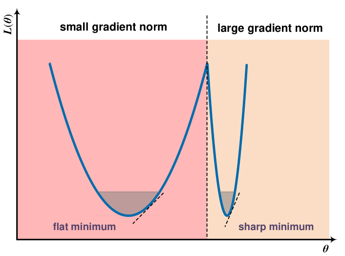
Figure 1: Toy example illustrating connections between the gradient norm of a function and the flatness of the function landscape.

In this paper, in addition to optimizing the common loss function, we would further impose an extra penalty on a specific property, the gradient norm of the loss function. The motivation of penalizing the gradient norm of loss function is to encourage the optimizer to find a minimum that lies in a relatively flat neighborhood region, since such flat minima have been demonstrated to be able to lead to better model generalization than sharp ones (Hochreiter & Schmidhuber, 1997). Figure 1 gives a toy example that illustrates the association between gradient norm and flatness of minima intuitively, and we would further demonstrate this from the perspective of Lipschitz continuity in Section 3.2.

Unfortunately, for practical implementation, optimizing the gradient norm in a straightforward way would involve the full calculation of Hessian matrix, which is not feasible for current hardwares. Here, by leveraging the approximation techniques, we present a simple and efficient scheme for computing the gradient of this gradient norm. The scheme would avoid the computation of the second-order derivative, and instead use basic algebraic operations between only the first-order derivatives for approximation, thus it could be implemented in practice easily. In particular, we find that the sharpness-aware minimization (SAM) scheme (Foret et al., 2021) is actually one special case of our scheme, where the hyperparameters are set to specific values.

In our experiments, we apply extensive model architectures on Cifar-{10, 100} datasets and ImageNet datasets, respectively. These models would include both simple and complex convolutional neural network architectures, as well as the recent vision transformer architectures. We observe that the model performance could be generally improved via our optimization scheme, and such improvements could be up to 70% greater than SAM’s improvements over the standard training. Also, in some cases, training could be more stable when using our scheme compared to the SAM scheme. Finally, we provide a guide on hyperparameter selection in expectation to achieve the best improvements in practice.

2 Related Works

Reguralization techniques

Regularization could widely refer to techniques that in some way help improve the model generalization, including penalty function methods (Smith et al., 1997), data augmentation (Devries & Taylor, 2017; Cubuk et al., 2018), dropout regularizations (Srivastava et al., 2014; Wan et al., 2013), normalization techniques (Ioffe & Szegedy, 2015; Ba et al., 2016; Wu & He, 2018) and so on. For penalty function methods, extra terms would be added and optimized along with the loss function, which targets to impose constraint on specific property of models. In particular, the weight norm has been demonstrated to be an important property related to the model capacity (Neyshabur et al., 2017), and penalizing the weight $L^{2}$-norm (Krogh & Hertz, 1991; Loshchilov & Hutter, 2019) has become, in a sense, the essential ingredient in modern training recipes. Others like Yoshida & Miyato (2017) penalize the spectral norm of weights for reducing the models’ sensitivity to input perturbation.

Flat minima

On the other hand, our work is also relevant to the research of flat minima. In Hochreiter & Schmidhuber (1997), the authors first point out that well generalized models may have flat minima. Since then, the association between flatness of minima and model generalization have been studied from both empirical (Keskar et al., 2017) and theoretical perspectives (Dinh et al., 2017; Neyshabur et al., 2017). Although SGD optimizer and some of its variants (such as momentum) could somehow serve as implicit regularizations that favors flat minima (Goodfellow et al., 2016; Wu et al., 2018; Xie et al., 2021), researchers also desire to bias the optimizers in an explicit way in pursuit of smoother surface and flatter minima to further improve model performance, especially for modern scalable models. But in practical optimization, explicitly finding flat minima is nontrivial. Recently, Foret et al. (2021) treat it as a minimax optimization problem, and solve it by introducing an efficient procedure, called SAM. Model generalization could be improved significantly compared to using vanilla SGD optimizations. Further, based on Foret et al. (2021), Kwon et al. (2021) propose the Adaptive SAM, where optimization could keep invariant to a specific weight-rescaling operation discussed in (Neyshabur et al., 2015; Dinh et al., 2017); Zheng et al. (2021) perform gradient descent twice in one step to solve the corresponding minimax problem, one for the inner maximization optimization and the other for the outer minimization optimization.

3 Method

3.1 Basic Setting

Given a training dataset ${\mathcal{S}}=\{({\bm{x}}_{i},{\bm{y}}_{i})\}_{i=0}^{n}$ drawn i.i.d from the distribution $\mathscr{D}$, a neural network $f(\cdot;{\bm{\theta}})$ is trained to learn this distribution. The neural network is parametrized with parameters ${\bm{\theta}}$ in weight space $\mathbf{\Theta}$, which would be optimized via minimizing an empirical loss function $L_{{\mathcal{S}}}({\bm{\theta}})=\frac{1}{N}\sum_{i=1}^{N}l(\hat{{\bm{y}}}_{i},{\bm{y}}_{i},{\bm{\theta}})$ where $\hat{{\bm{y}}}_{i}=f({\bm{x}}_{i};{\bm{\theta}})$ denoting the predicted label for input ${\bm{x}}_{i}$.

When imposing penalty on the gradient norm of the loss function, a term with respect to it could be added on the loss function $L_{{\mathcal{S}}}({\bm{\theta}})$ simply,

$$L({\bm{\theta}})=L_{{\mathcal{S}}}({\bm{\theta}})+\lambda\cdot||\nabla_{{\bm{\theta}}}L_{{\mathcal{S}}}({\bm{\theta}})||_{p}$$ (1)

where $||\cdot||_{p}$ denotes the $L^{p}$-norm and $\lambda$ is the penalty coefficient and $\lambda\in{\mathbb{R}}_{+}$ (in the experiment section, we also investigate the results where $\lambda\in{\mathbb{R}}_{-}$). And for clarity, we would use $L^{2}$-norm ($p=2$) in the following demonstration since it is the most commonly used metric in deep learning.

3.2 Gradient Norm and Lipschitz Continuity

Generally, penalizing the gradient norm of loss function would motivate the loss function to have small Lipschitz constant in local. If the loss function has a smaller Lipschitz constant, it would indicate that the loss function landscape is flatter, which in consequence could lead to better model generalization.

Regarding the term ”flat minima”, it is a rather intuitive concept. Based on the description in (Hochreiter & Schmidhuber, 1997), a flat minimum denotes ”a large connected region in weight space where the error remains approximately constant”. However, the mathematical descriptions may differ (Hochreiter & Schmidhuber, 1997; Neyshabur et al., 2017; Dinh et al., 2017; Keskar et al., 2017; Chaudhari et al., 2017), although they may convey similar core ideas. Here, we would only follow the basic concept in our demonstration.

We would start from the Lipschitz continuous. Given $\Omega\subset{\mathbb{R}}^{n}$, for function $h:\Omega\rightarrow{\mathbb{R}}^{m}$, it is called Lipschitz continuous if there exists a constant $K$ that satisfies,

$$||h({\bm{\theta}}_{1})-h({\bm{\theta}}_{2})||_{2}\leq K\cdot\|{\bm{\theta}}_{1}-{\bm{\theta}}_{2}||_{2}$$ (2)

for $\forall{\bm{\theta}}_{1},{\bm{\theta}}_{2}\in\Omega$. And the Lipschitz constant generally refers to the smallest $K$ of the function. Further, for $\forall{\bm{\theta}}\in\Omega$, $h$ is locally Lipschitz continuous if ${\bm{\theta}}$ has a neighborhood ${\mathcal{A}}$ that $h|_{{\mathcal{A}}}$ is Lipschitz continuous.

Intuitively, the Lipschitz constant describes the upper bound on the output change in the input space $\Omega$. In particular, for $h|_{{\mathcal{A}}}$, it would indicate the supremum of output change in the neighborhood ${\mathcal{A}}$. In other words, for small Lipschitz constants, given any two points in ${\mathcal{A}}$, the gap between their outputs is limited to a small range. In fact, this is essentially a kind of description of ”flat minima”.

So for a minimum ${\bm{\theta}}_{i}$ and the loss function $L({\bm{\theta}})$, according to the mean value theorem, the differentiability could lead to that for $\forall{\bm{\theta}}_{i}^{{}^{\prime}}\in{\mathcal{A}}$,

$$\|L({\bm{\theta}}_{i}^{{}^{\prime}})-L({\bm{\theta}}_{i})\|_{2}=\|\nabla L({\bm{\zeta}})({\bm{\theta}}_{i}^{{}^{\prime}}-{\bm{\theta}}_{i})\|_{2}$$ (3)

where ${\bm{\zeta}}=c{\bm{\theta}}_{i}+(1-c){\bm{\theta}}_{i}^{{}^{\prime}}$, $c\in[0,1]$. And the Cauchy-Schwarz inequality gives,

$$\|L({\bm{\theta}}_{i}^{{}^{\prime}})-L({\bm{\theta}}_{i})\|_{2}\leq\|\nabla L({\bm{\zeta}})\|_{2}\|({\bm{\theta}}_{i}^{{}^{\prime}}-{\bm{\theta}}_{i})\|_{2}$$ (4)

When ${\bm{\theta}}_{i}^{{}^{\prime}}\rightarrow{\bm{\theta}}$, the corresponding Lipschitz constant approximates to $\|\nabla L({\bm{\theta}}_{i})\|_{2}$. Therefore, we would expect to reduce $\|\nabla L({\bm{\theta}}_{i})\|_{2}$ to give small Lipschitz constants such that models could converge to flat minima.

Additionally, it should be especially discriminated that some works (Yoshida & Miyato, 2017; Virmaux & Scaman, 2018) try to regularize the Lipschitz constant of DNNs in the input space such that models would be more stable to the perturbation in the input space. This is not the same as penalizing the gradient norm of loss function, which would function in the weight space.

3.3 Gradient Calculation of Loss with Gradient Norm Penalty

During practical optimization, we need to calculate the gradient of current loss (Equation 1),

$$\nabla_{{\bm{\theta}}}L({\bm{\theta}})=\nabla_{{\bm{\theta}}}L_{{\mathcal{S}}}({\bm{\theta}})+\nabla_{{\bm{\theta}}}(\lambda\cdot||\nabla_{{\bm{\theta}}}L_{{\mathcal{S}}}({\bm{\theta}})||_{p})$$ (5)

Based on the chain rule, Equation 5 could be simplified as,

$$\nabla_{{\bm{\theta}}}L({\bm{\theta}})=\nabla_{{\bm{\theta}}}L_{{\mathcal{S}}}({\bm{\theta}})+\lambda\cdot\nabla_{{\bm{\theta}}}^{2}L_{{\mathcal{S}}}({\bm{\theta}})\frac{\nabla_{{\bm{\theta}}}L_{{\mathcal{S}}}({\bm{\theta}})}{||\nabla_{{\bm{\theta}}}L_{{\mathcal{S}}}({\bm{\theta}})||}$$ (6)

In Appendix, we have provided detailed procedures for this simplification from Equation 5 to Equation 6.

Apparently, Equation 6 involves the calculation of Hessian matrix. For DNNs, it is infeasible to straightforwardly solve such a Hessian matrix since the dimension in weight space is too huge. Appropriate approximation method should be implemented in this calculation.

In Equation 6, the Hessian matrix is essentially a linear operator ${\bm{H}}(\cdot)$ that functions on the corresponding gradient vector. Here, local Taylor expansion would be employed to approximate the operation results between the Hessian matrix and the gradient vector. From the Taylor expansion, we have

$$\nabla_{{\bm{\theta}}}L_{\mathcal{S}}({\bm{\theta}}+\Delta{\bm{\theta}})=\nabla_{{\bm{\theta}}}L_{\mathcal{S}}({\bm{\theta}})+{\bm{H}}\Delta{\bm{\theta}}+{\mathcal{O}}(||\Delta{\bm{\theta}}||^{2})$$ (7)

When choosing $\Delta{\bm{\theta}}=r{\bm{v}}$ where $r$ is a small value and ${\bm{v}}$ is a vector, Equation 7 would be,

$${\bm{H}}{\bm{v}}=\frac{\nabla_{{\bm{\theta}}}L_{\mathcal{S}}({\bm{\theta}}+r{\bm{v}})-\nabla_{{\bm{\theta}}}L_{\mathcal{S}}({\bm{\theta}})}{r}+{\mathcal{O}}(r)$$ (8)

Further, assigning ${\bm{v}}=\frac{\nabla_{{\bm{\theta}}}L_{{\mathcal{S}}}({\bm{\theta}})}{||\nabla_{{\bm{\theta}}}L_{{\mathcal{S}}}({\bm{\theta}})||}$,

$${\bm{H}}\frac{\nabla_{{\bm{\theta}}}L_{{\mathcal{S}}}({\bm{\theta}})}{||\nabla_{{\bm{\theta}}}L_{{\mathcal{S}}}({\bm{\theta}})||}\approx\frac{\nabla_{{\bm{\theta}}}L({\bm{\theta}}+r\frac{\nabla_{{\bm{\theta}}}L_{{\mathcal{S}}}({\bm{\theta}})}{||\nabla_{{\bm{\theta}}}L_{{\mathcal{S}}}({\bm{\theta}})||})-\nabla_{{\bm{\theta}}}L({\bm{\theta}})}{r}$$ (9)

Now, based on Equation 9, Equation 6 would be,

$$\begin{split}\nabla_{{\bm{\theta}}}L({\bm{\theta}})&=\nabla_{{\bm{\theta}}}L_{{\mathcal{S}}}({\bm{\theta}})\\ &+\frac{\lambda}{r}\cdot(\nabla_{{\bm{\theta}}}L_{\mathcal{S}}({\bm{\theta}}+r\frac{\nabla_{{\bm{\theta}}}L_{{\mathcal{S}}}({\bm{\theta}})}{||\nabla_{{\bm{\theta}}}L_{{\mathcal{S}}}({\bm{\theta}})||})-\nabla_{{\bm{\theta}}}L_{\mathcal{S}}({\bm{\theta}}))\\ &=(1-\alpha)\nabla_{{\bm{\theta}}}L_{{\mathcal{S}}}({\bm{\theta}})\\ &+\alpha\nabla_{{\bm{\theta}}}L_{\mathcal{S}}({\bm{\theta}}+r\frac{\nabla_{{\bm{\theta}}}L_{{\mathcal{S}}}({\bm{\theta}})}{||\nabla_{{\bm{\theta}}}L_{{\mathcal{S}}}({\bm{\theta}})||})\\ \end{split}$$ (10)

where $\alpha=\frac{\lambda}{r}$, and we would call $\alpha$ the balance coefficient.

Accordingly, we need to set two basic parameters $\lambda$ and $r$ to perform gradient norm penalty. For $\lambda$, it denotes the penalty coefficient, which controls the degree of the regularization on the gradient norm. However, the connections between weight norm, gradient norm and model generalization is subtle during training. Currently, how much the gradient norm should be penalized in practical training still requires some further tuning effort. As for $r$, it is used for appropriating the Hessian multiplication operation (Equation 8). Notably, $r$ should be set carefully here since it would directly affect the approximation precision (Pearlmutter, 1994). On the one hand, $r$ is expected to be small enough such that the term ${\mathcal{O}}(r)$ in approximation could be safely ignored. But on the other hand, as $r$ becomes smaller, the perturbed weight ${\bm{\theta}}+r{\bm{v}}$ will gradually weaken the effect of ${\bm{v}}$ and approach the reference weight ${\bm{\theta}}$, which makes $\nabla_{{\bm{\theta}}}L_{\mathcal{S}}({\bm{\theta}}+r{\bm{v}})$ and $\nabla_{{\bm{\theta}}}L_{\mathcal{S}}({\bm{\theta}})$ too close when appropriating ${\bm{H}}{\bm{v}}$. Therefore, we should also avoid setting $r$ too small to provide enough precision of ${\bm{v}}$.

In practice, we would further take an approximation for computing the second term in Equation 10 to avoid the Hessian computation caused by the chain rule,

$$\nabla_{{\bm{\theta}}}L_{\mathcal{S}}({\bm{\theta}}+r\frac{\nabla_{{\bm{\theta}}}L_{{\mathcal{S}}}({\bm{\theta}})}{||\nabla_{{\bm{\theta}}}L_{{\mathcal{S}}}({\bm{\theta}})||})\approx\nabla_{{\bm{\theta}}}L_{{\mathcal{S}}}({\bm{\theta}})|_{{\bm{\theta}}={\bm{\theta}}+r\frac{\nabla_{{\bm{\theta}}}L_{{\mathcal{S}}}({\bm{\theta}})}{||\nabla_{{\bm{\theta}}}L_{{\mathcal{S}}}({\bm{\theta}})||}}$$ (11)

Algorithm 1 Optimization Scheme of Penalizing Gradient Norm

Input: Training set ${\mathcal{S}}=\{({\bm{x}}_{i},{\bm{y}}_{i})\}_{i=0}^{N}$; loss function $L(\cdot)$; batch size $B$; learning rate $\eta$; total step $T$; balance coefficient $\alpha$; approximation scalar $r$.
Parameter: Model parameters ${\bm{\theta}}$
Output: Optimized weight $\hat{{\bm{\theta}}}$

1:  Parameter initialization ${\bm{\theta}}_{0}$.

2:  for step $t=1$ to $T$ do

3:     Get batch data pairs ${\mathcal{B}}=\{({\bm{x}}_{i},{\bm{y}}_{i})\}_{i=0}^{B}$ sampled from training set ${\mathcal{S}}$.

4:     Calculate the gradient ${\bm{g}}_{1}=\nabla_{{\bm{\theta}}}L_{\mathcal{S}}({\bm{\theta}})$ based on the batch samples.

5:     Add $r\frac{\nabla_{{\bm{\theta}}}L_{{\mathcal{S}}}({\bm{\theta}})}{||\nabla_{{\bm{\theta}}}L_{{\mathcal{S}}}({\bm{\theta}})||}$ on the current parameter ${\bm{\theta}}_{t}$, which makes ${\bm{\theta}}_{t}{{}^{\prime}}={\bm{\theta}}_{t}+r\frac{\nabla_{{\bm{\theta}}}L_{{\mathcal{S}}}({\bm{\theta}})}{||\nabla_{{\bm{\theta}}}L_{{\mathcal{S}}}({\bm{\theta}})||}$.

6:     Calculate the gradient ${\bm{g}}_{2}=\nabla_{{\bm{\theta}}}L_{{\mathcal{S}}}({\bm{\theta}})$ at ${\bm{\theta}}={\bm{\theta}}_{t}{{}^{\prime}}$.

7:     Calculate the final gradient ${\bm{g}}=(1-\alpha){\bm{g}}_{1}+\alpha{\bm{g}}_{2}$.

8:     (SGD optimizer) Update parameter with final gradient, ${\bm{\theta}}_{k+1}={\bm{\theta}}_{k}-\eta\cdot{\bm{g}}$.

9:  end for

10:  return Final optimization $\hat{{\bm{\theta}}}$.

Table 1: Testing error rate of CNN models on Cifar10 and Cifar100 when implementing the three training schemes.

	Cifar10		Cifar100
VGG16	Basic	Cutout	Basic	Cutout
Standard	$\ 7.07\$	$\ 5.31\$	$\ 28.78\$	$\ {\color[rgb]{1,0,0}\mathbf{26.98}}\$
SAM	$\ 6.91\$	$\ {\color[rgb]{1,0,0}\mathbf{6.17}}\$	$\ 28.62\$	$\ 27.13\$
Ours	$\ \ \mathbf{6.72}\ \$	$\ \ \mathbf{5.19}\ \$	$\ \ \mathbf{28.48}\ \$	$\ \ 27.07\ \$
VGG16-BN	Basic	Cutout	Basic	Cutout
Standard	$\ 5.74_{\pm 0.09}\$	$\ 4.39_{\pm 0.07}\$	$\ 25.22_{\pm 0.31}\$	$\ 24.69_{\pm 0.25}\$
SAM	$\ 5.24_{\pm 0.08}\$	$\ 4.16_{\pm 0.11}\$	$\ 24.23_{\pm 0.29}\$	$\ 23.35_{\pm 0.33}\$
Ours	$\ \ \mathbf{4.88_{\pm 0.12}}\ \$	$\ \ \mathbf{4.02_{\pm 0.08}}\ \$	$\ \ \mathbf{24.04_{\pm 0.18}}\ \$	$\ \ \mathbf{23.07_{\pm 0.26}}\ \$
WideResNet-28-10	Basic	Cutout	Basic	Cutout
Standard	$\ 3.53_{\pm 0.10}\$	$\ 2.81_{\pm 0.07}\$	$\ 18.99_{\pm 0.12}\$	$\ 16.92_{\pm 0.10}\$
SAM	$\ 2.78_{\pm 0.07}\$	$\ 2.43_{\pm 0.13}\$	$\ 16.53_{\pm 0.13}\$	$\ 14.87_{\pm 0.16}\$
Ours	$\ \ \mathbf{2.52_{\pm 0.09}}\ \$	$\ \ \mathbf{2.16_{\pm 0.11}}\ \$	$\ \ \mathbf{16.02_{\pm 0.19}}\ \$	$\ \ \mathbf{14.28_{\pm 0.16}}\ \$
WideResNet-SS 2$\times$96	Basic	Cutout	Basic	Cutout
Standard	$\ 2.82_{\pm 0.05}\$	$\ 2.39_{\pm 0.06}\$	$\ 17.19_{\pm 0.19}\$	$\ 15.85_{\pm 0.14}\$
SAM	$\ 2.37_{\pm 0.09}\$	$\ 2.11_{\pm 0.13}\$	$\ 15.22_{\pm 0.19}\$	$\ 14.32_{\pm 0.15}\$
Ours	$\ \ \mathbf{2.28_{\pm 0.13}}\ \$	$\ \ \mathbf{2.01_{\pm 0.10}}\ \$	$\ \ \mathbf{14.93_{\pm 0.10}}\ \$	$\ \ \mathbf{14.03_{\pm 0.17}}\ \$
PyramidNet-SD	Auto Aug + Cutmix		Auto Aug + Cutmix
Standard	$1.66_{\pm 0.11}$		$10.83_{\pm 0.14}$
SAM	$1.41_{\pm 0.08}$		$10.33_{\pm 0.13}$
Ours	$\mathbf{1.30_{\pm 0.07}}$		$\mathbf{10.12_{\pm 0.17}}$

In summary, Algorithm 1 gives the full procedures of our optimization scheme. It should be mentioned that Algorithm 1 only shows our scheme when using SGD optimizer. For other optimizers or update strategies (such as Adam), one could add specific operations before step 8.

Particularly, if $\alpha=1$, it is actually the SAM optimization (Foret et al., 2021). This indicates that SAM is a special implementation of penalizing gradient norm, where the penalty coefficient $\lambda$ is always set equal to $r$. However, given the distinct roles of the two parameters, we can not anticipate that models would achieve best performance every time at $\lambda=r$. Such a binding deployment, while reducing one parameter, also limits our tuning. We would further show that SAM could not be the best implementation in the following experiment section.

4 Experiments

We would demonstrate the effectiveness of our proposed scheme by investigating performance on image classification tasks. In all our experiments, we would compare our scheme with two other training schemes, one is the standard training scheme and the other one is the SAM training scheme. Besides, all the experiments are deployed using the JAX framework on the NVIDIA DGX Station A100.

4.1 Cifar10 and Cifar100

In this section, we would use Cifar10 and Cifar100 as our experimental datasets, and would separately apply the convolutional neural network (CNN) architectures and the vision transformer (ViT) architecture for the corresponding benchmark performance tests.

Convolutional neural network

For CNN architectures, five different architectures would be involved, including relatively simple architectures (VGG16 (Simonyan & Zisserman, 2015)) and complex architectures (WideResNet (Zagoruyko & Komodakis, 2016) and PyramidNet (Han et al., 2017)).

For training datasets, we would employ two kinds of augmentations. The first one is the basic augmentation, where samples are padded with additional four pixels on each boundary, randomly flipped in horizontal and then cropped randomly to size $32\times 32$. The second one is the cutout augmentation, where cutout regularization (Devries & Taylor, 2017) would be implemented moreover based on the basic augmentation. Specifically, cutout regularization is a common data augmentation technique for CNNs, which randomly masks out a square region in the input with a given mask value (generally zero).

Our investigation would focus on the comparisons between three different training schemes, namely the standard SGD scheme, SAM scheme and our scheme. Considering the connections between these three training schemes, we would adopt a ”greedy” strategy to reduce tuning cost during implementation,

1. We would first train models using the standard training scheme ($\lambda=0$ in our scheme), and record the common training hyperparameters (such as learning rate, weight decay) that could give the best model performance.

2. Based on the best hyperparameters recorded in Step 1, we would then set the balance coefficient $\alpha=1$ to train the same models using the SAM scheme, and perform a grid search on the parameter $r$.

3. Finally, based on the previous information, we would further perform a grid search on the balance coefficient $\alpha$ to adjust the penalty coefficient.

Basically, the involved model architectures have been extensively studied for the standard training scheme. It is not necessary to perform a heavy grid search, and we could just follow the common hyperparameters used in the related literatures. Next, we would perform a grid search on the scaler $r$ over the set $\{0.01,0.02,0.05,0.1,0.2\}$. This setting is actually the same as it in (Foret et al., 2021). And for a fair comparison, we would train the models to reach at comparable results as reported in their paper. After determining the best value of $r$, we would moreover perform a grid search on the balance coefficient $\alpha$ in the range 0.1 to 0.9 at an interval of 0.1.

For each model, we would train with five different random seeds, and record the convergence model performance on testing sets during training. And then we would report the mean value and the standard deviation, as shown in Table 1.

In table 1, totally five model cases are involved: the original VGG16 architecture and that with batch normalization regularization, the WideResNet-28-10 architecture and that with Shake-Shake regularization (Gastaldi, 2017), and the PyramidNet-272 architecture with Shake-Drop regularization (Yamada et al., 2019). We could see that for our training scheme, the model performance could be improved to some extent compared to the other two schemes.

For the original VGG16 model, training could frequently fail with relatively large learning rate, sometimes all five trials may fail especially for the SAM scheme. However, small learning rate may not lead to the best performance. Here, we would simply report the best training case (possibly trained more than five times and not following the greed strategy strictly).

Basically, the results are quite close when using the three training schemes. But it should be highly noted about the results when implementing cutout augmentation. On Cifar10, the performance using SAM scheme may be much worse than that using standard scheme. This is because that for the optimal common training hyperparameters in the standard scheme, all of the values in our grid search on approximation scalar $r$ fail to train from the start using SAM scheme. We have to lower the learning rate to stabilize the training. In contrast, by setting appropriate balance coefficient $\alpha$, our scheme could utilize the optimal common training hyperparameters, which could improve the performance slightly. However, on Cifar100, the standard training would yield the best performance.

When applying the batch normalization regularization on the VGG model, such training failures would be largely alleviated, although they may still happen in few trials. We would see that with batch normalization, VGG16 could receive significantly performance gains. The best performances are achieved via our scheme, which could be as low as 4% testing error rate on Cifar10.

As for the WideResNet architecture, we could find that our scheme could significantly improve the performance by 1% on Cifar10 and near 3% on Cifar100 compared to the standard training scheme. Our improvements could be 38% on average and up to remarkable 70% (on Cifar10 with cutout, ours is 0.65 while SAM’s is 0.38, which is $0.65=(1+71\%)\times 0.38$) more than the SAM’s improvements over the standard training scheme. This confirms the effectiveness of our scheme, and further demonstrates that SAM is not the best case in our scheme.

Regarding the WideResNet with Shake-Shake regularization (WideResNet-SS in the table), our improvements could not be as significant as that on the WideResNet architecture, but still give about 20% improvement compared to the SAM’s improvement over the standard training scheme.

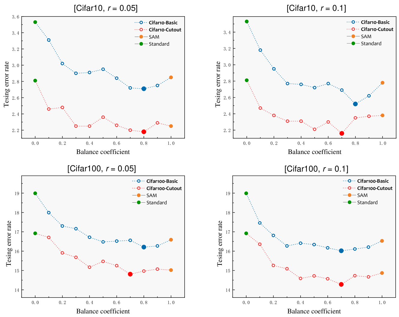
Figure 2: Testing error rate when trained with different hyperparameter $r$ and $\alpha$. The upper row denotes the error rate on Cifar10 while the lower row denotes the error rate on Cifar100, and the left column denotes $r=0.05$ while the right column denotes $r=0.1$. The points colored green are results using the standard scheme, and the points colored orange are results using the SAM scheme.

Finally, we would investigate the PyramidNet architecture with the Shake-Drop regularization (PyramidNet-SD in the table). We would adopt the auto-augmentation policy (Cubuk et al., 2018) and the cutmix regularization (Yun et al., 2019) for data augmentation. Here, only three random seeds are used for training. We could see that our scheme again improves the performance on both Cifar10 and Cifar100.

Vision transformer

We would like to investigate the effectiveness of our scheme on the recent vision transformer architectures (Dosovitskiy et al., 2021). Our investigation would focus on the ViT-TI16 and ViT-S16 architectures introduced in their paper.

Table 2: Testing error rate of ViT models on Cifar10 dataset when implementing the three training schemes.

	Cifar10
ViT-TI16	Basic	Heavy
Standard	$\ 15.92_{\pm 0.17}\$	$\ 14.68_{\pm 0.14}\$
SAM	$\ 15.33_{\pm 0.18}\$	$\ 13.77_{\pm 0.12}\$
Ours	$\ \mathbf{14.75_{\pm 0.17}}\$	$\ \mathbf{13.52_{\pm 0.21}}\$
ViT-S16	Basic	Heavy
Standard	$\ 14.55_{\pm 0.14}\$	$\ 13.31_{\pm 0.11}\$
SAM	$\ 13.91_{\pm 0.18}\$	$\ 12.63_{\pm 0.09}\$
Ours	$\ \mathbf{13.66_{\pm 0.16}}\$	$\ \mathbf{12.29_{\pm 0.19}}\$

Table 3: Testing error rate of ViT models on Cifar100 dataset when implementing the three training schemes.

	Cifar100
ViT-TI16	Basic	Heavy
Standard	$\ 40.21_{\pm 0.20}\$	$\ 38.93_{\pm 0.28}\$
SAM	$\ 38.89_{\pm 0.23}\$	$\ 37.61_{\pm 0.19}\$
Ours	$\ \mathbf{38.58_{\pm 0.27}}\$	$\ \mathbf{37.15_{\pm 0.21}}\$
ViT-S16	Basic	Heavy
Standard	$\ 38.43_{\pm 0.19}\$	$\ 37.58_{\pm 0.22}\$
SAM	$\ 37.98_{\pm 0.23}\$	$\ 36.77_{\pm 0.25}\$
Ours	$\ \mathbf{37.32_{\pm 0.28}}\$	$\ \mathbf{36.59_{\pm 0.22}}\$

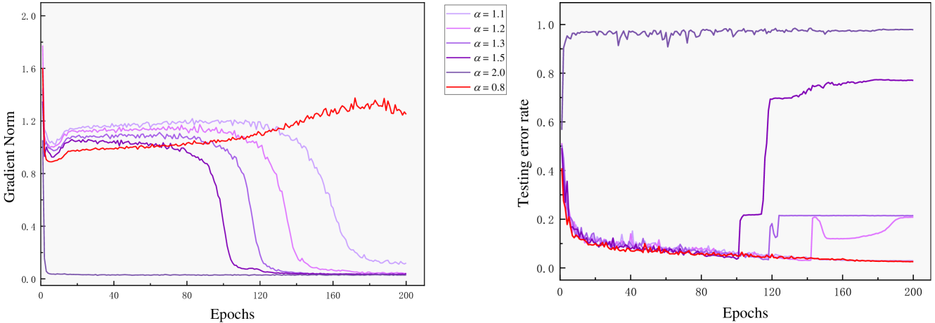
Figure 3: Evolutions of gradient norm of loss function (left) and testing error rate on Cifar10. Purple curves represent the results where $\alpha\in{\mathcal{B}}_{b}$, while the red curve represents the optimal results where $\alpha=0.8$.

Here, we would adopt the same greedy search strategy as in the previous section for the three training schemes. Likewise, five random seeds are used for each model. But for data augmentation, we would not use cutout augmentation here since we find such augmentation would not boost the model performance. Intuitively, the vision transformer architecture would cut the image into small patches, and utilize the relationship between these patches to make decisions. In this way, the cutout regularization may not be helpful for models to learn the relationship between patches. Here, we would replace the cutout augmentation with a heavy augmentation, considering that vision transformer architectures are generally data hungry models. In the heavy augmentation, we would perform a series of operations, including resizing to $72\times 72$, random flipping, random rotating, random zooming, random cropping and finally resizing to $48\times 48$. We would adopt the $4\times 4$ patch size in both the basic augmentation and the heavy augmentation. Models would be trained much longer using heavy augmentation than those using basic augmentation (1200 v.s 300 epochs). In addition, we would use extra operations like label smoothing and drop path as used in (Dosovitskiy et al., 2021) when using the heavy augmentation.

Table 2 & 3 presents the corresponding testing error rate. We could see that even if using heavy augmentation, the performances of vision transformer architectures would be much worse than those of CNN architectures. And in the table, we could find that the performances could be improved via implementing our scheme. This further confirms the broad applicability of our scheme.

Parameter study

Further, we would investigate the impact on model performance as choosing different balance coefficients $\alpha$ and approximation scalars $r$ in our optimization scheme, which we would illustrate using the WideResNet-28-10 model architecture.

When performing the grid search on approximate value $r$ in the SAM training experiments, we observe that models would have relatively better performances when setting $r=0.05$ and $r=0.1$. This observation is the same as that in (Foret et al., 2021). Then, the grid search over balance coefficient $\alpha$ is performed moreover based on $r=0.05$ and $0.1$. Figure 2 shows the results. In Figure 2, rows denote results on Cifar10 and Cifar100, respectively, and blue lines in the plots denote adopting basic data augmentation while red lines denote adopting cutout data augmentation. As we would see in the figure, from the standard training scheme ($\alpha=0$) to the SAM training scheme ($\alpha=1$), each curve may experience a decrease and then an increase in the testing error rate. Based on the figure, we could find that these models would achieve best performance when the balance coefficient $\alpha$ is set around 0.7 or 0.8.

In addition to the basic set in the previous deployment of $\alpha$, we would like to further investigate cases where $\alpha\notin[0,1]$. Extra deployments would be implemented over two other sets, ${\mathcal{B}}_{a}=\{-0.1,-0.2,-0.5\}$ and ${\mathcal{B}}_{b}=\{1.1,1.2,1.3,1.5,2.0\}$.

For ${\mathcal{B}}_{a}$, since its values are all negative, this causes that the penalty coefficient of gradient norm in Equation 1 becomes negative, which makes it a reward as increasing the gradient norm during optimization. Generally, if $\lambda\leq 0$, the optimization would not be fully ensured, since we are adding a negative term on the loss. And in all of our trials, no matter trained on Cifar10 or Cifar100 datasets, the models completely fail to converge even if gradient clip regularization is adopted. The gradient would be unstable, and may even explode immediately after the training start. But this instead shows the effectiveness of our penalty scheme.

As for ${\mathcal{B}}_{b}$, since the values in it are all greater than 1.0, the penalty on the gradient norm becomes larger, and the operation relationship in Equation 10 shifts from addition to subtraction. This may somehow be harmful to training, as shown in figure 3. In the figure, the left plot denotes the gradient norm of loss function with respect to the training epochs, while the right plot denotes the testing error rate on Cifar10 datasets.

We could find that these large coefficients indeed impose much heavier penalties on the gradient norm of loss function. The gradient norm would drop faster and faster as $\alpha$ increases from 1.1 to 2.0. For $\alpha=2.0$, the gradient norm would drop to near zero immediately after the training start. As for other values in ${\mathcal{B}}_{b}$, although the gradient norm would keep stable for a while, it would suddenly drop rapidly within only several epochs. As soon as the gradient norm begins to drop rapidly, the testing error rate would increase immediately. When the gradient norms reach near zero, the testing error rates become stable. Interestingly, the final convergence error rates may be different even though the corresponding gradient norms are all near zero.

In summary, one should impose the penalty on the gradient norm with appropriate parameters in practice, where $\alpha=0.8$ and $r\in\{0.05,0.1\}$ are highly recommended for achieving the best performance. Based on our observation, this deployment could also give the best performance for most of our training, not just the WideResNet-28-10 architecture.

4.2 ImageNet

Next, we would check the effectiveness of our scheme on the large-scale dataset, namely ImageNet. For model architectures, we would adopt the VGG16-BN, ResNet50 and ResNet101 in our investigation. Likewise, we would still adopt the three training schemes for comparisons. However, unlike using the greedy strategy for hyperparameter searching in the previous section, we would directly set $r=0.05$ according to (Foret et al., 2021) and perform only a slight grid search on $\alpha$ over $\{0.7,0.8\}$ based on our parameter study. For data augmentation, we just follow the prior works (He et al., 2016; Simonyan & Zisserman, 2015). Here, we would train each model with three different random seeds. Besides, all models are trained within 100 epochs with a cosine learning rate schedule.

Table 4: Testing error rate of models on ImageNet dataset when implementing the three training schemes.

	ImageNet
VGG16-BN	Top-1 Accuracy	Top-5 Accuracy
Standard	$\ 26.89_{\pm 0.12}\$	$\ 8.88_{\pm 0.06}\$
SAM	$\ 26.41_{\pm 0.13}\$	$\ 8.60_{\pm 0.05}\$
Ours	$\ \mathbf{26.12_{\pm 0.16}}\$	$\ \mathbf{8.44_{\pm 0.06}}\$
ResNet50	Top-1 Accuracy	Top-5 Accuracy
Standard	$\ 23.64_{\pm 0.17}\$	$\ 7.01_{\pm 0.09}\$
SAM	$\ 23.16_{\pm 0.11}\$	$\ 6.72_{\pm 0.06}\$
Ours	$\ \mathbf{22.87_{\pm 0.15}}\$	$\ \mathbf{6.59_{\pm 0.11}}\$
ResNet101	Top-1 Accuracy	Top-5 Accuracy
Standard	$\ 21.97_{\pm 0.09}\$	$\ 6.11_{\pm 0.07}\$
SAM	$\ 21.02_{\pm 0.10}\$	$\ 5.31_{\pm 0.09}\$
Ours	$\ \mathbf{20.53_{\pm 0.13}}\$	$\ \mathbf{5.18_{\pm 0.08}}\$

Table 4 reports top-1 and top-5 testing error rates for different models. As we could see in the table, the model generalization could be improved when using our scheme compared to the other two schemes. Again, this confirms the effectiveness of our scheme for practical training.

5 Conclusion

In this paper, we introduce an effective scheme for penalizing the gradient norm of loss function during training optimization. In our scheme, no Hessian computation would be involved, making it efficient to be implemented in practical optimization. We confirm the effectiveness of our training scheme via image classification experiments which involve extensive model architecture on commonly used datasets. By comparing with two baselines (the standard training scheme and SAM scheme) on Cifar and ImageNet dataset, we show the superiority of our scheme, where several new state-of-art performances are achieved. Remarkably, the improvement of using our scheme may be at most 70% greater than that of using the SAM scheme. Also, we perform a parameter study to guide the setting of optimal hyperparameters in practice. It is shown that one should carefully set the parameters, in case of losing precision of approximation during penalty.

Appendix A Simplification Process of Equation 6

The Equation 6 is,

$$\nabla_{{\bm{\theta}}}L({\bm{\theta}})=\nabla_{{\bm{\theta}}}L_{{\mathcal{S}}}({\bm{\theta}})+\nabla_{{\bm{\theta}}}(\lambda\cdot||\nabla_{{\bm{\theta}}}L_{{\mathcal{S}}}({\bm{\theta}})||_{p})$$ (12)

where would like to simply the second term $\nabla_{{\bm{\theta}}}(\lambda\cdot||\nabla_{{\bm{\theta}}}L_{{\mathcal{S}}}({\bm{\theta}})||_{2})$.

For ${\bm{\theta}}=[\theta_{1},\theta_{2},\cdots,\theta_{n}]^{\intercal}$, the 2-norm function is,

$$g({\bm{\theta}}):=||{\bm{\theta}}||_{2}=\sqrt{\theta_{1}^{2}+\theta_{2}^{2}+\cdots+\theta_{n}^{2}}$$ (13)

The partial derivative of $g({\bm{\theta}})$ with respect to $\theta_{i}$ denotes,

$$\frac{\partial g({\bm{\theta}})}{\partial\theta_{i}}=\frac{\theta_{i}}{\sqrt{\theta_{1}^{2}+\theta_{2}^{2}+\cdots+\theta_{n}^{2}}}=\frac{\theta_{i}}{||{\bm{\theta}}||_{2}}=\frac{\theta_{i}}{g({\bm{\theta}})}$$ (14)

Therefore,

$$\nabla_{{\bm{\theta}}}g({\bm{\theta}})=[\frac{\theta_{1}}{g({\bm{\theta}})},\frac{\theta_{2}}{g({\bm{\theta}})},\cdots,\frac{\theta_{n}}{g({\bm{\theta}})}]^{\intercal}$$ (15)

The gradient of ${\bm{\theta}}$ denotes $h({\bm{\theta}}):=\nabla_{{\bm{\theta}}}L({\bm{\theta}})$. And the term $\nabla_{{\bm{\theta}}}(||\nabla_{{\bm{\theta}}}L({\bm{\theta}})||_{2})$ could be simplified as,

$$\begin{split}\nabla_{{\bm{\theta}}}(||\nabla_{{\bm{\theta}}}L({\bm{\theta}})||_{2})&=\nabla_{{\bm{\theta}}}(g\circ h)({\bm{\theta}})\\ &=(\nabla_{{\bm{\theta}}}g({\bm{\zeta}})|_{{\bm{\zeta}}=h({\bm{\theta}})})\cdot(\nabla_{{\bm{\theta}}}h({\bm{\theta}}))\\ &=(\frac{{\bm{\zeta}}}{g({\bm{\zeta}})}|_{{\bm{\zeta}}=h({\bm{\theta}})})\cdot(\nabla_{{\bm{\theta}}}h({\bm{\theta}}))\\ &=(\frac{\nabla_{{\bm{\theta}}}L({\bm{\theta}})}{||\nabla_{{\bm{\theta}}}L({\bm{\theta}})||_{2}})\cdot(\nabla^{2}L({\bm{\theta}}))\\ &=\frac{1}{||\nabla_{{\bm{\theta}}}L({\bm{\theta}})||_{2}}\cdot\nabla^{2}L({\bm{\theta}})\cdot\nabla_{{\bm{\theta}}}L({\bm{\theta}})\end{split}$$ (16)

Back to Equation 6, the equation could be simplified based on Equation 16,

$$\begin{split}\nabla_{{\bm{\theta}}}L({\bm{\theta}})&=\nabla_{{\bm{\theta}}}L_{{\mathcal{S}}}({\bm{\theta}})+\nabla_{{\bm{\theta}}}(\lambda\cdot||\nabla_{{\bm{\theta}}}L_{{\mathcal{S}}}({\bm{\theta}})||_{p})\\ &=\nabla_{{\bm{\theta}}}L_{{\mathcal{S}}}({\bm{\theta}})+\lambda\cdot\nabla^{2}L_{{\mathcal{S}}}({\bm{\theta}})\cdot\frac{\nabla_{{\bm{\theta}}}L_{{\mathcal{S}}}({\bm{\theta}})}{||\nabla_{{\bm{\theta}}}L_{{\mathcal{S}}}({\bm{\theta}})||_{2}}\end{split}$$ (17)

References

- Ba et al. (2016) Ba, L. J., Kiros, J. R., and Hinton, G. E. Layer normalization. arXivPreprint, abs/1607.06450, 2016.
- Chaudhari et al. (2017) Chaudhari, P., Choromanska, A., Soatto, S., LeCun, Y., Baldassi, C., Borgs, C., Chayes, J. T., Sagun, L., and Zecchina, R. Entropy-sgd: Biasing gradient descent into wide valleys. In 5th International Conference on Learning Representations, ICLR 2017. OpenReview.net, 2017.
- Cubuk et al. (2018) Cubuk, E. D., Zoph, B., Mané, D., Vasudevan, V., and Le, Q. V. Autoaugment: Learning augmentation policies from data. arXivPreprint, abs/1805.09501, 2018.
- Devries & Taylor (2017) Devries, T. and Taylor, G. W. Improved regularization of convolutional neural networks with cutout. arXivPreprint, abs/1708.04552, 2017.
- Dinh et al. (2017) Dinh, L., Pascanu, R., Bengio, S., and Bengio, Y. Sharp minima can generalize for deep nets. In Proceedings of the 34th International Conference on Machine Learning, ICML 2017, volume 70, pp. 1019–1028, 2017.
- Dosovitskiy et al. (2021) Dosovitskiy, A., Beyer, L., Kolesnikov, A., Weissenborn, D., Zhai, X., Unterthiner, T., Dehghani, M., Minderer, M., Heigold, G., Gelly, S., Uszkoreit, J., and Houlsby, N. An image is worth 16x16 words: Transformers for image recognition at scale. In 9th International Conference on Learning Representations, ICLR 2021, 2021.
- Foret et al. (2021) Foret, P., Kleiner, A., Mobahi, H., and Neyshabur, B. Sharpness-aware minimization for efficiently improving generalization. In 9th International Conference on Learning Representations, ICLR 2021, 2021.
- Gastaldi (2017) Gastaldi, X. Shake-shake regularization of 3-branch residual networks. In 5th International Conference on Learning Representations, ICLR 2017, Workshop Track Proceedings, 2017.
- Goodfellow et al. (2016) Goodfellow, I. J., Bengio, Y., and Courville, A. C. Deep Learning. Adaptive computation and machine learning. MIT Press, 2016. ISBN 978-0-262-03561-3.
- Goyal et al. (2017) Goyal, P., Dollár, P., Girshick, R. B., Noordhuis, P., Wesolowski, L., Kyrola, A., Tulloch, A., Jia, Y., and He, K. Accurate, large minibatch SGD: training imagenet in 1 hour. arXivPreprint, abs/1706.02677, 2017.
- Han et al. (2017) Han, D., Kim, J., and Kim, J. Deep pyramidal residual networks. In 2017 IEEE Conference on Computer Vision and Pattern Recognition, CVPR 2017, pp. 6307–6315, 2017.
- He et al. (2016) He, K., Zhang, X., Ren, S., and Sun, J. Deep residual learning for image recognition. In 2016 IEEE Conference on Computer Vision and Pattern Recognition, CVPR 2016, pp. 770–778, 2016.
- Hochreiter & Schmidhuber (1997) Hochreiter, S. and Schmidhuber, J. Flat minima. Neural Comput., 9(1):1–42, 1997.
- Ioffe & Szegedy (2015) Ioffe, S. and Szegedy, C. Batch normalization: Accelerating deep network training by reducing internal covariate shift. In Proceedings of the 32nd International Conference on Machine Learning, ICML 2015, volume 37, pp. 448–456, 2015.
- Keskar et al. (2017) Keskar, N. S., Mudigere, D., Nocedal, J., Smelyanskiy, M., and Tang, P. T. P. On large-batch training for deep learning: Generalization gap and sharp minima. In 5th International Conference on Learning Representations, ICLR 2017, 2017.
- Krogh & Hertz (1991) Krogh, A. and Hertz, J. A. A simple weight decay can improve generalization. In Advances in Neural Information Processing Systems,, pp. 950–957, 1991.
- Kwon et al. (2021) Kwon, J., Kim, J., Park, H., and Choi, I. K. ASAM: adaptive sharpness-aware minimization for scale-invariant learning of deep neural networks. In Proceedings of the 38th International Conference on Machine Learning, ICML 2021, volume 139 of Proceedings of Machine Learning Research, pp. 5905–5914, 2021.
- Loshchilov & Hutter (2019) Loshchilov, I. and Hutter, F. Decoupled weight decay regularization. In 7th International Conference on Learning Representations, ICLR 2019, 2019.
- Neyshabur et al. (2015) Neyshabur, B., Salakhutdinov, R., and Srebro, N. Path-sgd: Path-normalized optimization in deep neural networks. In Advances in Neural Information Processing, pp. 2422–2430, 2015.
- Neyshabur et al. (2017) Neyshabur, B., Bhojanapalli, S., McAllester, D., and Srebro, N. Exploring generalization in deep learning. In Advances in Neural Information Processing Systems, pp. 5947–5956, 2017.
- Pearlmutter (1994) Pearlmutter, B. A. Fast exact multiplication by the hessian. Neural Comput., 6(1):147–160, 1994.
- Simonyan & Zisserman (2015) Simonyan, K. and Zisserman, A. Very deep convolutional networks for large-scale image recognition. In 3rd International Conference on Learning Representations, ICLR 2015, 2015.
- Smith et al. (1997) Smith, A. E., Coit, D. W., Baeck, T., Fogel, D., and Michalewicz, Z. Penalty functions. Handbook of evolutionary computation, 97(1):C5, 1997.
- Srivastava et al. (2014) Srivastava, N., Hinton, G. E., Krizhevsky, A., Sutskever, I., and Salakhutdinov, R. Dropout: a simple way to prevent neural networks from overfitting. J. Mach. Learn. Res., 15(1):1929–1958, 2014.
- Virmaux & Scaman (2018) Virmaux, A. and Scaman, K. Lipschitz regularity of deep neural networks: analysis and efficient estimation. In Advances in Neural Information Processing Systems 31: Annual Conference on Neural Information Processing Systems 2018, NeurIPS 2018, pp. 3839–3848, 2018.
- Wan et al. (2013) Wan, L., Zeiler, M. D., Zhang, S., LeCun, Y., and Fergus, R. Regularization of neural networks using dropconnect. In Proceedings of the 30th International Conference on Machine Learning, ICML 2013, volume 28, pp. 1058–1066, 2013.
- Wu et al. (2018) Wu, L., Ma, C., and E, W. How SGD selects the global minima in over-parameterized learning: A dynamical stability perspective. In Advances in Neural Information Processing Systems 31: Annual Conference on Neural Information Processing Systems 2018, NeurIPS 2018, pp. 8289–8298, 2018.
- Wu & He (2018) Wu, Y. and He, K. Group normalization. In Computer Vision - ECCV 2018, volume 11217, pp. 3–19, 2018.
- Xie et al. (2021) Xie, Z., Sato, I., and Sugiyama, M. A diffusion theory for deep learning dynamics: Stochastic gradient descent exponentially favors flat minima. In 9th International Conference on Learning Representations, ICLR 2021,. OpenReview.net, 2021.
- Yamada et al. (2019) Yamada, Y., Iwamura, M., Akiba, T., and Kise, K. Shakedrop regularization for deep residual learning. IEEE Access, 7:186126–186136, 2019. ISSN 2169-3536.
- Yoshida & Miyato (2017) Yoshida, Y. and Miyato, T. Spectral norm regularization for improving the generalizability of deep learning. arXivPreprint, abs/1705.10941, 2017.
- Yun et al. (2019) Yun, S., Han, D., Chun, S., Oh, S. J., Yoo, Y., and Choe, J. Cutmix: Regularization strategy to train strong classifiers with localizable features. In 2019 IEEE/CVF International Conference on Computer Vision, ICCV 2019, pp. 6022–6031. IEEE, 2019.
- Zagoruyko & Komodakis (2016) Zagoruyko, S. and Komodakis, N. Wide residual networks. In Proceedings of the British Machine Vision Conference 2016, BMVC 2016, 2016.
- Zheng et al. (2021) Zheng, Y., Zhang, R., and Mao, Y. Regularizing neural networks via adversarial model perturbation. In IEEE Conference on Computer Vision and Pattern Recognition, CVPR 2021, pp. 8156–8165, 2021.