Convolutional Neural Networks on Graphs with Chebyshev Approximation, Revisited

Abstract

Designing spectral convolutional networks is a challenging problem in graph learning. ChebNet, one of the early attempts, approximates the spectral graph convolutions using Chebyshev polynomials. GCN simplifies ChebNet by utilizing only the first two Chebyshev polynomials while still outperforming it on real-world datasets. GPR-GNN and BernNet demonstrate that the Monomial and Bernstein bases also outperform the Chebyshev basis in terms of learning the spectral graph convolutions. Such conclusions are counter-intuitive in the field of approximation theory, where it is established that the Chebyshev polynomial achieves the optimum convergent rate for approximating a function.

In this paper, we revisit the problem of approximating the spectral graph convolutions with Chebyshev polynomials. We show that ChebNet’s inferior performance is primarily due to illegal coefficients learnt by ChebNet approximating analytic filter functions, which leads to over-fitting. We then propose ChebNetII, a new GNN model based on Chebyshev interpolation, which enhances the original Chebyshev polynomial approximation while reducing the Runge phenomenon. We conducted an extensive experimental study to demonstrate that ChebNetII can learn arbitrary graph convolutions and achieve superior performance in both full- and semi-supervised node classification tasks. Most notably, we scale ChebNetII to a billion graph ogbn-papers100M, showing that spectral-based GNNs have superior performance. Our code is available at https://github.com/ivam-he/ChebNetII.

1 Introduction

Graph neural networks (GNNs) have received considerable attention in recent years due to their remarkable performance on a variety of graph learning tasks, including social analysis [31, 24, 38], drug discovery [49, 19, 32], traffic forecasting [26, 3, 7] and recommendation system [42, 46].

Spatial-based and spectral-based graph neural networks (GNNs) are the two primary categories of GNNs. To learn node representations, spatial-based GNNs [21, 15, 39] often rely on a message propagation and aggregation mechanism between neighboring nodes. Spectral-based methods [8, 12] create spectral graph convolutions or, equivalently, spectral graph filters, in the spectral domain of the graph Laplacian matrix. We can further divide spectral-based GNNs into two categories based on whether or not their graph convolutions can be learned.

• Predetermined graph convolutions: GCN [21] employs a simplified first tow Chebyshev polynomials as the graph convolution, which is a fixed low-pass filter [1, 41, 43, 54]. APPNP [22] and GDC [12] set the graph convolution with Personalized PageRank (PPR) and also achieve a low-pass filter. [12, 54]. S²GC [52] derives the graph convolution from the Markov Diffusion Kernel, which is a low- and high-pass filter trade-off. GNN-LF/HF [54] designs the graph convolutions from the perspective of graph optimization that can imitate low- and high-pass filters.

• Learnable graph convolutions: ChebNet [8] approximates the graph convolutions using Chebyshev polynomials and, in theory, could learn arbitrary filters [1]. CayleyNet [23] learns the graph convolutions with Cayley polynomials and generates various graph filters. GPR-GNN [6] uses the Monomial basis to approximate graph convolutions, which can derive low- or high-pass filters. ARMA [2] learns the rational graph convolutions through the Auto-Regressive Moving Average filters family [28]. BernNet [17] utilizes the Bernstein basis to approximate the graph convolutions, which can also learn arbitrary graph filters.

Despite the recent developments, two fundamental problems with spectral-based GNNs remain unsolved. First of all, it is well-known that GCN [21] outperforms ChebNet [8] on real-world datasets (e.g., semi-supervised node classification tasks on citation datasets [21]). However, it is also established that GCN is a simplified version of ChebNet with only the first two Chebyshev polynomials and that ChebNet has more expressive capability than GCN in theory [1]. Consequently, a natural question is: Why is ChebNet’s performance inferior to GCN’s despite its better expressiveness?

Secondly, as shown in [17], the real-world performance of ChebNet is also inferior to that of GPR-GNN [6] and BernNet [17], which use Monomial polynomial basis and Bernstein polynomial basis to approximate the spectral graph convolutions. Such a conclusion is counter-intuitive in the field of approximation theory, where it is established that the Chebyshev polynomial achieves near-optimum error when approximating a function [13]. Therefore, the second question is: Why is ChebNet’s filter inferior to that of GPR-GNN and BernNet, despite the fact that Chebyshev polynomials have a higher approximation ability?

In this paper, we attempt to tackle these problems by revisiting the fundamental problem of approximating the spectral graph convolutions with Chebyshev polynomials. First of all, according to the theory of the Chebyshev approximation, we observe that the coefficients of the Chebyshev expansion for an analytic function need to satisfy an inevitable convergence. Consequently, we prove that ChebNet’s inferior performance is primarily due to illegal coefficients learnt by ChebNet approximating analytic filter functions, which leads to over-fitting. Furthermore, we propose ChebNetII, a new GNN model based on Chebyshev interpolation, which enhances the original Chebyshev polynomial approximation while reducing the Runge phenomenon [10]. Our ChebNetII model has robust scalability and can easily cope with various constraints on the learned filters via simple reparameterization, such as the non-negativity constraints proposed in [17]. Finally, we conduct an extensive experimental study to demonstrate that ChebNetII can achieve superior performance in both full- and semi-supervised node classification tasks and scale to the billion graph ogbn-papers100M .

2 Revisiting ChebNet

Notations. We consider an undirected graph $G=(V,E)$ with node set $V$ and edge set $E$. Let $n=|V|$ denote the number of nodes. We use $\mathbf{x}\in\mathbb{R}^{n}$ to denote the graph signal, where $\mathbf{x}(i)$ denotes the signal at node $i$. Note that in the general case of GNNs where the input feature is a matrix $\mathbf{X}$, we can treat each column of $\mathbf{X}$ as a graph signal. Let $\mathbf{A}$ denote the adjacency matrix and $\mathbf{D}$ denote the diagonal degree matrix, where $\mathbf{D}_{ii}=\sum\nolimits_{j}^{n}\mathbf{A}_{ij}$. For convenience, we use $\mathbf{P}=\mathbf{D}^{-1/2}\mathbf{A}\mathbf{D}^{-1/2}$ and $\mathbf{L}=\mathbf{I}-\mathbf{D}^{-1/2}\mathbf{A}\mathbf{D}^{-1/2}$ to denote the normalized adjacency matrix and the normalized Laplacian matrix of $G$, respectively. We use $\mathbf{L}=\mathbf{U}\mathbf{\Lambda}\mathbf{U}^{T}$ to represent the eigendecomposition of $\mathbf{L}$, where $\mathbf{U}$ denotes the matrix of eigenvectors and $\mathbf{\Lambda}=\textit{diag}[\lambda_{1},...,\lambda_{n}]$ is the diagonal matrix of eigenvalues.

2.1 Spectral-based GNNs and ChebNet

Spectral-based GNNs create the spectral graph convolutions in the domain of Laplacian spectrum. Recent studies suggest that many popular methods use the polynomial spectral filters to achieve graph convolutions [8, 21, 17]. We can formulate this polynomial filtering operation as

$$\mathbf{y}=\mathbf{U}diag\left[h(\lambda_{1}),...,h(\lambda_{n})\right]\mathbf{U}^{T}\mathbf{x}=\mathbf{U}h\left(\mathbf{\Lambda}\right)\mathbf{U}^{T}\mathbf{x}\approx\sum\limits_{k=0}^{K}w_{k}\mathbf{L}^{k}\mathbf{x},$$ (1)

where $\mathbf{y}$ denotes the filtering results of $\mathbf{x}$, and $h(\lambda)$ is called the spectral filter, which is a function of eigenvalues of the Laplacian matrix $\mathbf{L}$. The $w_{k}$ denote the polynomial filter weights, and the polynomial filter can be defined as $h(\lambda)=\sum\nolimits_{k=0}^{K}w_{k}\lambda^{k},\lambda\in[0,2]$. ChebNet [8] is a remarkable attempt in this field, which uses Chebyshev polynomial to approximate the filtering operation.

$$\mathbf{y}\approx\sum\limits_{k=0}^{K}w_{k}T_{k}(\hat{\mathbf{L}})\mathbf{x},$$ (2)

where $\hat{\mathbf{L}}=2\mathbf{L}/\lambda_{max}-\mathbf{I}$ denotes the scaled Laplacian matrix. $\lambda_{max}$ is the largest eigenvalue of $\mathbf{L}$ and $w_{k}$ denote the Chebyshev coefficients. The Chebyshev polynomials can be recursively defined as $T_{k}(x)=2xT_{k-1}(x)-T_{k-2}(x)$, with $T_{0}(x)=1$ and $T_{1}(x)=x$. ChebNet’s structure is:

$$\mathbf{Y}=\sum\limits_{k=0}^{K}T_{k}(\hat{\mathbf{L}})\mathbf{X}\mathbf{W}_{k},$$ (3)

with the trainable weights $\mathbf{W}_{k}$. The Chebyshev coefficients $w_{k}$ of the filtering operation (2) are implicitly encoded in the weight matrices $\mathbf{W}_{k}$. We list more spectral-based GNNs’ details in Appendix A.

Table 1: Comparison of ChebNet and GCN.

Method	Cora	Citeseer	Pubmed
ChebNet (2)	80.54${}_{\pm\text{0.38}}$	70.35${}_{\pm\text{0.33}}$	75.52${}_{\pm\text{0.75}}$
ChebNet (10)	74.91${}_{\pm\text{0.52}}$	67.69${}_{\pm\text{0.64}}$	65.91${}_{\pm\text{1.71}}$
GCN	81.32${}_{\pm\text{0.18}}$	71.77${}_{\pm\text{0.21}}$	79.15${}_{\pm\text{0.18}}$

Table 2: Comparison of different bases.

Method	Cora	Citeseer	Pubmed
ChebBase	79.29${}_{\pm\text{0.36}}$	70.76${}_{\pm\text{0.37}}$	78.07${}_{\pm\text{0.32}}$
GPR-GNN	83.95${}_{\pm\text{0.22}}$	70.92${}_{\pm\text{0.57}}$	78.97${}_{\pm\text{0.27}}$
BernNet	83.15${}_{\pm\text{0.32}}$	72.24${}_{\pm\text{0.25}}$	79.65${}_{\pm\text{0.25}}$

2.2 The motivation of revisiting ChebNet

ChebNet versus GCN. Even though GCN is a simplified form of ChebNet, it is well known that ChebNet is inferior to GCN for semi-supervised node classification tasks [21]. Table 2.1 shows the results of ChebNet and GCN for semi-supervised node classification tasks on Cora, Citeseer and Pubmed datasets (see Appendix E for experimental details) . We find that ChebNet is inferior to GCN, especially when we increase the polynomial order $K$ from $2$ to $10$ in Equation (3).

On the other hand, existing research [1] has shown that ChebNet is more expressive than GCN in theory. In particular, ChebNet can approximate arbitrary spectral filters as $K$ increases, while GCN is a fixed low-pass filter. If we set $K=1$ and $w_{0}=w_{1}$ in the Equation (2), ChebNet corresponds to a high-pass filter; if we set $K=1$ and $w_{0}=-w_{1}$, ChebNet becomes a low-pass filter which is essentially the same as GCN. Consequently, a natural question is: Why is ChebNet’s performance inferior to GCN’s despite its better expressiveness?

Chebyshev basis versus other bases. Chebyshev polynomials are widely used to approximate various functions in the digital signal processing and the graph signal filtering [36, 37]. The truncated Chebyshev expansions are demonstrated to produce a minimax polynomial approximation for the analytic functions [13]. Consequently, the spectral filters can be well-approximated by a truncated expansion in terms of Chebyshev polynomials $T_{k}(x)$ up to $K$-th order [16].

$$h(\hat{\lambda})\approx\sum\limits_{k=0}^{K}w_{k}T_{k}(\hat{\lambda}),\hat{\lambda}\in[-1,1],$$ (4)

where $\hat{\lambda}$ is the eigenvalue of the scaled Laplacian matrix $\mathbf{\hat{\mathbf{L}}}$. ChebNet [8] then defined the graph convolutions using the Chebyshev approximated filters, while recent works were inspired by ChebNet and used Monomial (i.e., GPR-GNN [6]) and Bernstein (i.e., BernNet [17]) bases to approximate filters. In order to evaluate the approximation ability of Chebyshev basis, we propose ChebNet with explicit coefficients, ChebBase, which simply replaces the Monomial basis of GPR-GNN and Bernstein basis of BernNet with the Chebyshev basis. The expression of ChebBase is

$$\mathbf{Y}=\sum\limits_{k=0}^{K}w_{k}T_{k}(\hat{\mathbf{L}})f_{\theta}\left(\mathbf{X}\right),$$ (5)

where $f_{\theta}(\mathbf{X})$ denotes Multi-Layer Perceptron (MLP). Table 2.1 reveals the results of ChebBase, GPR-GNN and BernNet for node classification tasks on three citation graphs. We can observe that ChebBase has the worst performance, which is inconsistent with the fact that the Chebyshev basis can approximate minimax polynomial in theory. Therefore, the second question is: Why is ChebNet’s filter inferior to that of GPR-GNN and BernNet, despite the fact that Chebyshev polynomials have a higher approximation ability?

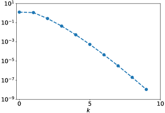
(a) Chebyshev coefficients of $exp({\hat{\lambda}})$.

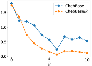
(b) Chebyshev coefficients learnt on Cora.

Figure 1: Illustrations of the Chebyshev expansion’s coefficients of $exp({\hat{\lambda}})$ and the Chebyshev coefficients learnt by ChebBase and ChebBase/$k$ on Cora.

2.3 Coefficient Constraints

We now demonstrate that ChebNet’s suboptimal performance is due to the illegal coefficients learned, which results in over-fitting. Given an arbitrary continuous function $f(x)$ in the interval $[-1,1]$, the Chebyshev expansion is defined as $f(x)=\sum\nolimits_{k=0}^{\infty}w_{k}T_{k}(x)$ with the Chebyshev coefficients $w_{k}$. The following theorem establishes that in order to approximate an analytic function, the Chebyshev expansion’s coefficients must be constrained.

Theorem 2.1.

[48] If $f(x)$ is weakly singular at the boundaries and analytic in the interval $(-1,1)$, then the Chebyshev coefficients $w_{k}$ will asymptotically (as $k\to\infty$) decrease proportionally to $1/k^{q}$ for some positive constant $q$.

Here, "weakly singular" means that the derivative of $f$ could vanish at the boundaries, and "analytic" means $f$ can be locally given by a convergent power series in the interval $(-1,1)$. Intuitively, Chebyshev polynomial $T_{k}(x)$ with larger $k$ corresponds to higher frequency oscillation (see Appendix C for more details). Theorem 2.1 essentially demonstrates that high frequency polynomials should be constrained in the Chebyshev expansion to approximate an analytic function. Figure 1(a) depicts the Chebyshev expansion’s coefficients of the analytic function $exp(\hat{\lambda})$ used as a spectral filter in GDC [12] and shows that the coefficients are convergent.

Table 3: The performance of ChebBase.

Method	Cora	Citeseer	Pubmed
ChebNet	80.54${}_{\pm\text{0.38}}$	70.35${}_{\pm\text{0.33}}$	75.52${}_{\pm\text{0.75}}$
GCN	81.32${}_{\pm\text{0.18}}$	71.77${}_{\pm\text{0.21}}$	79.15${}_{\pm\text{0.18}}$
ChebBase	79.29${}_{\pm\text{0.36}}$	70.76${}_{\pm\text{0.37}}$	78.07${}_{\pm\text{0.32}}$
ChebBase$/k$	82.66${}_{\pm\textbf{0.28}}$	72.52${}_{\pm\textbf{0.29}}$	79.25${}_{\pm\textbf{0.31}}$

The ability to approximate an analytic function is crucial in the task of approximating the spectral filters, since non-analytic filters are more difficult to approximate by polynomials and may result in over-fitting. In particular, ChebNet and ChebBase learn the coefficients $w_{k}$ by gradient descent without any constraints. The coefficients may not satisfy Theorem 2.1, leading to their poor performance. To validate this conjuncture, we conducted an empirical analysis of ChebBase with difference coefficient constraints. Inspired by Theorem 2.1, we use the following propagation process for the ChebBase$/k$.

$$\mathbf{Y}=\sum\limits_{k=0}^{K}\frac{w_{k}}{k}T_{k}(\hat{\mathbf{L}})f_{\theta}\left(\mathbf{X}\right),$$ (6)

where $w_{k}/k$ denote the Chebyshev coefficients implemented by reparameterizing the learnable parameters $w_{k}$. Table 3 shows the experimental results of the semi-supervised node classification performed on the citation graphs. We can observe that with a simple penalty on $w_{k}$, ChebBase$/k$ outperforms ChebNet, ChebBase, and GCN. Figure 1(b) plots the absolute value of the Chebyshev coefficients learnt by ChebBase and ChebBase/$k$ on Cora. We can observe that the coefficients of ChebBase/$k$ could more readily satisfy the convergence constraint. These results validate Theorem 2.1.

3 ChebNetII model

Although ChebBase$/k$ appears to be a promising approach, it still has some drawbacks: 1) Imposing the penalty on the coefficients is not mathematically elegant, as Theorem 2.1 only provides a necessary condition for the coefficients; 2) It is hard to impose further constraints on the learned spectral filters. For example, it is unclear how we can modify Equation (6) to obtain non-negative filters, a requirement proposed in [17]. In this section, we describe ChebNetII, a GNN model based on Chebyshev interpolation that resolves the above two issues. We also discuss the advantages and disadvantages of various polynomial interpolations as well as the Runge phenomenon.

3.1 Chebyshev interpolation

Consider a real filter function $h(\hat{\lambda})$ that is continuous in the interval $[-1,1]$. When the values of this filter are known at a finite number of points $\hat{\lambda}_{k}$, one can consider the approximation by a polynomial $P_{K}$ with $K$ degree such that $h(\hat{\lambda}_{k})=P_{K}(\hat{\lambda}_{k})$, which is the general polynomial interpolation. We give an explicit expression of the general polynomial interpolation in Appendix D.

We generally sample the $K+1$ points $\hat{\lambda}_{0}<\hat{\lambda}_{1}<...<\hat{\lambda}_{K}$ uniformly from $[-1,1]$ to construct the interpolating polynomial $P_{K}(\hat{\lambda})$. Intuitively, increasing $K$ should improve the approximation quality. However, this is not always the case due to the Runge Phenomenon [10] (The details are discussed in section  3.3). The popular approach to this problem in the literature [14] is Chebyshev interpolation, having superior approximation ability and faster convergence. Instead of sampling the interpolation points uniformly, Chebyshev interpolation uses Chebyshev nodes as the interpolation points, which are essentially the zeros of the $(K+1)$-th Chebyshev polynomial.

Definition 3.1.

(Chebyshev Nodes) The Chebyshev polynomial $T_{k}(x)$ satisfies the closed form expression $T_{k}(x)=\cos\left(k\arccos(x)\right)$. The Chebyshev Nodes for $T_{k}(x)$ are defined as $x_{j}=\cos{\left(\frac{2j+1}{2k}\pi\right)},j=0,1,...,k-1$, which lie in the interval $(-1,1)$ and are the zeros of $T_{k}(x)$.

Definition 3.1 suggests that each Chebyshev polynomial $T_{k}(x)$ has $k$ zeros, and we can define Chebyshev interpolation by replacing the equispaced points with Chebyshev nodes in the general polynomial interpolation (see Appendix D for details). More eloquently, definition 3.2 efficiently defines the Chebyshev interpolation via their orthogonality properties.

Definition 3.2.

(Chebyshev Interpolation) [14] Given a continuous filter function $h(\hat{\lambda})$, let $x_{j}=cos\left(\frac{j+1/2}{K+1}\pi\right),j=0,\ldots,K$ denote the Chebyshev nodes for $T_{K+1}$ and $h(x_{j})$ denotes the function value at node $x_{j}$. The Chebyshev interpolation of $h(\hat{\lambda})$ is defined to be

$$P_{K}(\hat{\lambda})=\sum\limits_{k=0}^{K}c_{k}^{\prime}T_{k}(\hat{\lambda}),c_{k}=\frac{2}{K+1}\sum\limits_{j=0}^{K}h(x_{j})T_{k}(x_{j}),$$ (7)

where the prime indicates the first term is to be halved, that is, $c_{0}^{\prime}=c_{0}/2$, $c_{1}^{\prime}=c_{1},\ldots,c_{K}^{\prime}=c_{K}$.

3.2 ChebNetII via Chebyshev Interpolation

Inspired by Chebyshev interpolation, we propose ChebNetII, a graph convolutional network that approximates an arbitrary spectral filter $h(\hat{\lambda})$ with an optimal convergence rate. ChebNetII simply reparameterizes the filter value $h(x_{j})$ in Equation (7) as a learnable parameter $\gamma_{j}$, which allows the model to learn an arbitrary spectral filter via gradient descent. More precisely, the ChebNetII model can be formulated as

where $x_{j}=cos\left(\left(j+1/2\right)\pi/(K+1)\right)$ are the Chebyshev nodes of $T_{K+1}$, $f_{\theta}(\mathbf{X})$ denotes an MLP on the node feature matrix $\mathbf{X}$, and $\gamma_{j}$ for $j=0,1,...,K$ are the learnable parameters. Note that similar to APPNP [22], we decouple feature propagation and transformation.

Consequently, the filtering operation of ChebNetII can be expressed as

$$\mathbf{y}\approx\frac{2}{K+1}\sum\limits_{k=0}^{K}\sum\limits_{j=0}^{K}\gamma_{j}T_{k}(x_{j})T_{k}(\hat{\mathbf{L}})\mathbf{x}.$$ (9)

It is easy to see that compared to the filtering operation of the original ChebNet (2), we only make one simple change: reparameterizing the coefficient $w_{k}$ by $w_{k}=\frac{2}{K+1}\sum\nolimits_{j=0}^{K}\gamma_{j}T_{k}(x_{j})$. However, this simple modification allows us to have more control on shaping the resulting filter, as Chebyshev interpolation suggests that $\gamma_{j}$ directly corresponds to the filter value $h(x_{j})$ at the Chebyshev node $x_{j}$. The coefficients $w_{k}=\frac{2}{K+1}\sum\nolimits_{j=0}^{K}h(x_{j})T_{k}(x_{j})$ are fundamentally guaranteed to satisfy the constraints of Theorem 2.1 since we directly approximate the filter $h$. Furthermore, Chebyshev interpolation also provides the ChebNetII with several beneficial mathematical properties.

Table 4: Dataset statistics.

	Chameleon	Squirrel	Actor	Texas	Cornell	Cora	Citeseer	Pubmed	ogbn-arxiv	ogbn-papers100M
Nodes	2277	5201	7600	183	183	2708	3327	19,717	169,343	111,059,956
Edges	31,371	198,353	26,659	279	277	5278	4552	44,324	1,166,243	1,615,685,872
Features	2325	2089	932	1703	1703	1433	3703	500	128	128
Classes	5	5	5	5	5	7	6	5	40	172
$\mathcal{H}(G)$	0.23	0.22	0.22	0.11	0.30	0.81	0.74	0.80	0.66	-

3.3 Analysis of ChebNetII

ChebNetII has several advantages over existing GNN models due to the unique nature of Chebyshev interpolation. From the standpoint of polynomial approximation and computational complexity, we compare ChebNetII with current related approaches such as GPR-GNN [6] and BernNet [17].

Near-minimax approximation. First of all, we examine ChebNetII’s capabilities in terms of filter function approximation. Theorem 3.1 exhibits that ChebNetII provides an approximation that is close to the best polynomial approximation for a spectral filter $h$.

Theorem 3.1.

[27] A polynomial approximation $P^{\ast}_{K}(x)$ for a function $f(x)$ is said to be near-best/minimax approximation with a relative distance $\rho$ if

$$||f(x)-P^{\ast}_{K}(x)||\leq(1+\rho)||f(x)-P^{\ast}_{B}(x)||,$$ (10)

where $\rho$ is the Lebesgue constant, $P^{\ast}_{B}(x)$ is a best polynomial approximation, and $||\cdot||$ represents the uniform norm (i.e., $||g||=\max_{x\in[-1,1]}|g(x)|$). Then, we have $\rho\sim 2^{K}$ as $K\to\infty$ for the general polynomial interpolation, and $\rho\sim\log(K)$ as $K\to\infty$ for the Chebyshev interpolation.

Convergence. In comparison to BernNet [17], which uses the Bernstein basis, ChebNetII has a faster convergence rate for approximating a filter function. Specifically, we have the following Theorem:

Theorem 3.2.

[14, 29] Let $P_{K}(x)$ be the polynomial approximation for a function $f(x)$. Then the error is given as $||f(x)-P_{K}(x)||\leq E(K)$. If $P_{K}(x)$ is obtained by Bernstein approximation, then $E(K)\sim(1+(2K)^{-2})\omega(K^{-1/2})$; if $P_{K}(x)$ is obtained by Chebyshev Interpolation, then $E(K)\sim C\omega(K^{-1})\log(K)$ with a constant $C$, where $\omega$ is the modulus of continuity.

Runge phenomenon. In comparison to GPR-GNN [6], which uses the Monomial basis, ChebNetII has the advantage of reducing the Runge phenomenon [10]. In particular, when we use the general polynomial interpolation to approximate a Runge filter $h(\hat{\lambda})$ with a high degree over a set of equispaced interpolation points, it will cause oscillation along the edges of an interval. Consequently, as the degree of the polynomial increases, the interpolation error increases. Following [14], we define the error of polynomial interpolation as

$$R_{K}(\hat{\lambda})=h(\hat{\lambda})-P_{K}(\hat{\lambda})=\frac{h^{K+1}(\zeta)}{(K+1)!}\pi_{K+1}(\hat{\lambda}),$$ (11)

where $\pi_{K+1}(\hat{\lambda})=\prod\nolimits_{k=0}^{K}(\hat{\lambda}-\hat{\lambda}_{k})$ denotes the nodal polynomial and $\zeta$ is the value depending on $\hat{\lambda}$. The terrible Runge phenomenon is caused by the values of this nodal polynomial, which have very high oscillations around the interval endpoints. In particular, for high-degree polynomial interpolation at equidistant points in $[-1,1]$, we have $\lim_{K\rightarrow\infty}\left(\max_{-1\leq\hat{\lambda}\leq 1}|R_{K}(\hat{\lambda})|\right)=\infty.$

On the other hand, we have the following Theorem 3.3 that explains that Chebyshev nodes can minimize and quantify this error caused by the nodal polynomial, meaning Chebyshev interpolation minimizes the problem of the Runge phenomenon.

Theorem 3.3.

[14] Consider the Chebyshev nodes $x_{j}=cos\left(\left(j+1/2\right)\pi/(K+1)\right)$, $j=0,1,...,K$. Then the nodal polynomial $\hat{T}_{K+1}(x)=\prod\nolimits_{k=0}^{K}(x-x_{j})$ has the smallest possible uniform norm, i.e., $||\hat{T}_{K+1}(x)||=2^{-K}$.

Computational complexity. Compared to BernNet [17], which has a time complexity quadratic to the order $K$ in the forward process, ChebNetII can be computed in time linear to $K$. Specifically, we first compute the ChebNetII’s coefficients $\frac{2}{K+1}\sum\nolimits_{j=0}^{K}\gamma_{j}T_{k}(x_{j})$ in time linear to $K$ as we can precompute $T_{k}(x_{j})$, and then plug the coefficients into Equation (8) for propagation, which also takes the time linear to $K$, the same as that of ChebNet [8] and GPR-GNN [6].

Table 5: Dataset statistics of large heterophilic graphs.

	Penn94	pokec	arXiv-year	genius	twitch-gamers	wiki
Nodes	41,554	1,632,803	169,343	421,961	168,114	1,925,342
Edges	1,362,229	30,622,564	1,166,243	984,979	6,797,557	303,434,860
Features	5	65	128	12	7	600
Classes	2	2	5	2	2	5
$\mathcal{H}(G)$	0.47	0.46	0.22	0.62	0.55	0.39

4 Experiments

In this section, we conduct experiments to evaluate the performance of ChebNetII against the state-of-the-art graph neural networks on a wide variety of open graph datasets.

Dataset and Experimental setup. We evaluate ChebNetII on several real-world graphs for the Semi- and Full-supervised node classification tasks. The datasets include three homophilic citation graphs: Cora, Citeseer, and Pubmed [35, 45], five heterophilic graphs: the Wikipedia graphs Chameleon and Squirrel [34], the Actor co-occurrence graph, and webpage graphs Texas and Cornell from WebKB [30], two large citation graphs: ogbn-arxiv and ogbn-papers100M [18], as well as six large heterophilic graphs: Penn94, pokec, arXiv-year, genius, twitch-gamers and wiki [25]. We measure the level of homophily in a graph using the edge homophily ratio $\mathcal{H}(G)=\frac{|\{(u,v):(u,v)\in E\wedge y_{v}=y_{u}\}|}{|E|}$ [53], where $y_{v}$ denotes the label of node $v$. We summarize the dataset statistics in Tables 4 and  5. All the experiments are carried out on a machine with an NVIDIA RTX8000 GPU (48GB memory), Intel Xeon CPU (2.20 GHz) with 40 cores, and 512 GB of RAM.

4.1 Semi-supervised node classification with polynomial-based methods

Setting and baselines. For the semi-supervised node classification task, we compare ChebNetII to 7 polynomial approximation filter methods, including MLP, GCN [21], ARMA [2], APPNP [22], ChebNet [8], GPR-GNN [6] and BernNet [17]. For dataset splitting, we employ both random and fixed splits and report the results on random splits. The results of fixed splits will be discussed in Appendix E.2. Specifically, we apply the standard training/validation/testing split [45] on the three homophilic citation datasets (i.e., Cora, Citeseer, and Pubmed), with 20 nodes per class for training, 500 nodes for validation, and 1,000 nodes for testing. Since this standard split can not be used for very small graphs (e.g. Texas), we use the sparse splitting [6] with the training/validation/test sets accounting for 2.5%/2.5%/95%, respectively, on the five heterophilic datasets.

For ChebNetII, we use Equation (8) as the propagation process and use the $ReLu$ function to reparametrize $\gamma_{j}$, maintaining the non-negativity of the filters [17]. We set the hidden units as 64 and $K=10$ for the all datasets as the same as GPR-GNN [6] and BernNet [17]. We employ the Adam SGD optimizer [20] with an early stopping of 200 and a maximum of 1000 epochs to train ChebNetII. We use the officially released code for GPR-GNN and BernNet and use the Pytorch Geometric library implementations [11] for other models (i.e., MLP, GCN, APPNP, ARMA, and ChebNet). More details of hyper-parameters and baselines’ settings are listed in Appendix E.2.

Results. We utilize accuracy (the micro-F1 score) with a 95% confidence interval as the evaluation metric. Table 6 reports the relevant results on 10 random splits. Boldface letters indicate the best result for the given confidence interval, and underlinings denote the next best result. We first observe that ChebNet is inferior to GCN even on heterophilic graphs, which concurs with our theoretical analysis that the illegal coefficients learned by ChebNet lead to over-fitting. ChebNetII, on the other hand, outperforms other methods on all datasets excluding Pubmed, where it also achieves top-2 classification accuracy. This quality is due to the fact that the learnable parameters $\gamma_{j}$ of ChebNetII directly correspond to the filter value $h(x_{j})$ at the Chebyshev node $x_{j}$, effectively preventing it from learning an illegal filter.

Table 6: Mean classification accuracy of semi-supervised node classification with random splits.

Method	Cham.	Squi.	Texas	Corn.	Actor	Cora	Cite.	Pubm.
MLP	26.36${}_{\pm\text{2.85}}$	21.42${}_{\pm\text{1.50}}$	32.42${}_{\pm\text{9.91}}$	36.53${}_{\pm\text{7.92}}$	29.75${}_{\pm\text{0.95}}$	57.17${}_{\pm\text{1.34}}$	56.75${}_{\pm\text{1.55}}$	70.52${}_{\pm\text{2.01}}$
GCN	38.15${}_{\pm\text{3.77}}$	31.18${}_{\pm\text{0.93}}$	34.68${}_{\pm\text{9.07}}$	32.36${}_{\pm\text{8.55}}$	22.74${}_{\pm\text{2.37}}$	79.19${}_{\pm\text{1.37}}$	69.71${}_{\pm\text{1.32}}$	78.81${}_{\pm\text{0.84}}$
ChebNet	37.15${}_{\pm\text{1.49}}$	26.55${}_{\pm\text{0.46}}$	36.35${}_{\pm\text{8.90}}$	28.78${}_{\pm\text{4.85}}$	26.58${}_{\pm\text{1.92}}$	78.08${}_{\pm\text{0.86}}$	67.87${}_{\pm\text{1.49}}$	73.96${}_{\pm\text{1.68}}$
ARMA	37.42${}_{\pm\text{1.72}}$	24.15${}_{\pm\text{0.93}}$	39.65${}_{\pm\text{8.09}}$	28.90${}_{\pm\text{10.07}}$	27.02${}_{\pm\text{2.31}}$	79.14${}_{\pm\text{1.07}}$	69.35${}_{\pm\text{1.44}}$	78.31${}_{\pm\text{1.33}}$
APPNP	32.73${}_{\pm\text{2.31}}$	24.50${}_{\pm\text{0.89}}$	34.79${}_{\pm\text{10.11}}$	34.85${}_{\pm\text{9.71}}$	29.74${}_{\pm\text{1.04}}$	82.39${}_{\pm\text{0.68}}$	69.79${}_{\pm\text{0.92}}$	79.97${}_{\pm\textbf{1.58}}$
GPR-GNN	33.03${}_{\pm\text{1.92}}$	24.36${}_{\pm\text{1.52}}$	33.98${}_{\pm\text{11.90}}$	38.95${}_{\pm\text{12.36}}$	28.58${}_{\pm\text{1.01}}$	82.37${}_{\pm\text{0.91}}$	69.22${}_{\pm\text{1.27}}$	79.28${}_{\pm\text{2.25}}$
BernNet	27.32${}_{\pm\text{4.04}}$	22.37${}_{\pm\text{0.98}}$	43.01${}_{\pm\text{7.45}}$	39.42${}_{\pm\text{9.59}}$	29.87${}_{\pm\text{0.78}}$	82.17${}_{\pm\text{0.86}}$	69.44${}_{\pm\text{0.97}}$	79.48${}_{\pm\text{1.47}}$
ChebNetII	43.42${}_{\pm\textbf{3.54}}$	33.96${}_{\pm\textbf{1.22}}$	46.58${}_{\pm\textbf{7.68}}$	42.19${}_{\pm\textbf{11.61}}$	30.18${}_{\pm\textbf{0.81}}$	82.42${}_{\pm\textbf{0.64}}$	69.89${}_{\pm\textbf{1.21}}$	79.51${}_{\pm\text{1.03}}$

Table 7: Mean classification accuracy of full-supervised node classification with random splits.

Method	Cham.	Squi.	Texas	Corn.	Actor	Cora	Cite.	Pubm.
MLP	46.59${}_{\pm\text{1.84}}$	31.01${}_{\pm\text{1.18}}$	86.81${}_{\pm\text{2.24}}$	84.15${}_{\pm\text{3.05}}$	40.18${}_{\pm\text{0.55}}$	76.89${}_{\pm\text{0.97}}$	76.52${}_{\pm\text{0.89}}$	86.14${}_{\pm\text{0.25}}$
GCN	60.81${}_{\pm\text{2.95}}$	45.87${}_{\pm\text{0.88}}$	76.97${}_{\pm\text{3.97}}$	65.78${}_{\pm\text{4.16}}$	33.26${}_{\pm\text{1.15}}$	87.18${}_{\pm\text{1.12}}$	79.85${}_{\pm\text{0.78}}$	86.79${}_{\pm\text{0.31}}$
ChebNet	59.51${}_{\pm\text{1.25}}$	40.81${}_{\pm\text{0.42}}$	86.28${}_{\pm\text{2.62}}$	83.91${}_{\pm\text{2.17}}$	37.42${}_{\pm\text{0.58}}$	87.32${}_{\pm\text{0.92}}$	79.33${}_{\pm\text{0.57}}$	87.82${}_{\pm\text{0.24}}$
ARMA	60.21${}_{\pm\text{1.00}}$	36.27${}_{\pm\text{0.62}}$	83.97${}_{\pm\text{3.77}}$	85.62${}_{\pm\text{2.13}}$	37.67${}_{\pm\text{0.54}}$	87.13${}_{\pm\text{0.80}}$	80.04${}_{\pm\text{0.55}}$	86.93${}_{\pm\text{0.24}}$
APPNP	52.15${}_{\pm\text{1.79}}$	35.71${}_{\pm\text{0.78}}$	90.64${}_{\pm\text{1.70}}$	91.52${}_{\pm\text{1.81}}$	39.76${}_{\pm\text{0.49}}$	88.16${}_{\pm\text{0.74}}$	80.47${}_{\pm\text{0.73}}$	88.13${}_{\pm\text{0.33}}$
GCNII	63.44${}_{\pm\text{0.85}}$	41.96${}_{\pm\text{1.02}}$	80.46${}_{\pm\text{5.91}}$	84.26${}_{\pm\text{2.13}}$	36.89${}_{\pm\text{0.95}}$	88.46${}_{\pm\text{0.82}}$	79.97${}_{\pm\text{0.65}}$	89.94${}_{\pm\textbf{0.31}}$
TWIRLS	50.21${}_{\pm\text{2.97}}$	39.63${}_{\pm\text{1.02}}$	91.31${}_{\pm\text{3.36}}$	89.83${}_{\pm\text{2.29}}$	38.13${}_{\pm\text{0.81}}$	88.57${}_{\pm\text{0.91}}$	80.07${}_{\pm\text{0.94}}$	88.87${}_{\pm\text{0.43}}$
EGNN	51.55${}_{\pm\text{1.73}}$	35.81${}_{\pm\text{0.91}}$	81.34${}_{\pm\text{1.56}}$	82.09${}_{\pm\text{1.16}}$	35.16${}_{\pm\text{0.64}}$	87.47${}_{\pm\text{1.33}}$	80.51${}_{\pm\text{0.93}}$	88.74${}_{\pm\text{0.46}}$
PDE-GCN	66.01${}_{\pm\text{1.56}}$	48.73${}_{\pm\text{1.06}}$	93.24${}_{\pm\text{2.03}}$	89.73${}_{\pm\text{1.35}}$	39.76${}_{\pm\text{0.74}}$	88.62${}_{\pm\text{1.03}}$	79.98${}_{\pm\text{0.97}}$	89.92${}_{\pm\text{0.38}}$
GPR-GNN	67.49${}_{\pm\text{1.38}}$	50.43${}_{\pm\text{1.89}}$	92.91${}_{\pm\text{1.32}}$	91.57${}_{\pm\text{1.96}}$	39.91${}_{\pm\text{0.62}}$	88.54${}_{\pm\text{0.67}}$	80.13${}_{\pm\text{0.84}}$	88.46${}_{\pm\text{0.31}}$
BernNet	68.53${}_{\pm\text{1.68}}$	51.39${}_{\pm\text{0.92}}$	92.62${}_{\pm\text{1.37}}$	92.13${}_{\pm\text{1.64}}$	41.71${}_{\pm\text{1.12}}$	88.51${}_{\pm\text{0.92}}$	80.08${}_{\pm\text{0.75}}$	88.51${}_{\pm\text{0.39}}$
ChebNetII	71.37${}_{\pm\textbf{1.01}}$	57.72${}_{\pm\textbf{0.59}}$	93.28${}_{\pm\textbf{1.47}}$	92.30${}_{\pm\textbf{1.48}}$	41.75${}_{\pm\textbf{1.07}}$	88.71${}_{\pm\textbf{0.93}}$	80.53${}_{\pm\textbf{0.79}}$	88.93${}_{\pm\text{0.29}}$

4.2 Full-supervised node classification

Setting and baselines. For full-supervised node classification, we compare ChebNetII to the baselines in the prior semi-supervised node classification. We also include GCNII [5], TWIRLS [44], EGNN [51] and PDE-GCN [9] four competitive baselines for full-supervised node classification. For all datasets, we randomly split the nodes into 60%, 20%, and 20% for training, validation and testing, and all methods share the same 10 random splits for a fair comparison, as suggested in [30, 6, 17].

For ChebNetII, we also set the hidden units to be 64 and $K=10$ for all datasets, and employ the same training manner as in the semi-supervised node classification task. For GCNII, TWIRLS, EGNN and PDE-GCN we use the officially released code. More details of hyper-parameters and baselines’ settings are listed in Appendix E.3.

Results. Table 7 reports the mean classification accuracy of each model. We first observe that, given more training data, ChebNet starts to outperform GCN on both homophilic and heterophilic datasets, which demonstrates the effectiveness of the Chebyshev approximation. However, we also observe that ChebNetII achieves new state-of-the-art results on 7 out of 8 datasets and competitive results on Pubmed. Notably, ChebNetII outperforms GPR-GNN and BernNet by over 10% on the Squirrel dataset. We attribute this quality to the fact that Chebyshev interpolation achieves near-minimax approximation of any function with respect to the uniform norm, giving ChebNetII greater approximation power than GPR-GNN and BernNet do.

Table 8: Experimental results on large heterophilic graphs. OOM denotes "out of memory".

Method	Penn94	pokec	arXiv-year	genius	twitch-gamers	wiki
MLP	73.61${}_{\pm\text{0.40}}$	62.37${}_{\pm\text{0.02}}$	36.70${}_{\pm\text{0.21}}$	86.68${}_{\pm\text{0.09}}$	60.92${}_{\pm\text{0.07}}$	37.38${}_{\pm\text{0.21}}$
LINK	80.79${}_{\pm\text{0.49}}$	80.54${}_{\pm\text{0.03}}$	53.97${}_{\pm\text{0.18}}$	73.56${}_{\pm\text{0.14}}$	64.85${}_{\pm\text{0.21}}$	57.11${}_{\pm\text{0.26}}$
LINKX	84.71${}_{\pm\text{0.52}}$	82.04${}_{\pm\text{0.07}}$	56.00${}_{\pm\textbf{1.34}}$	90.77${}_{\pm\text{0.27}}$	66.06${}_{\pm\textbf{0.19}}$	59.80${}_{\pm\text{0.41}}$
GCN	82.47${}_{\pm\text{0.27}}$	75.45${}_{\pm\text{0.17}}$	46.02${}_{\pm\text{0.26}}$	87.42${}_{\pm\text{0.37}}$	62.18${}_{\pm\text{0.26}}$	OOM
GCNII	82.92${}_{\pm\text{0.59}}$	78.94${}_{\pm\text{0.11}}$	47.21${}_{\pm\text{0.28}}$	90.24${}_{\pm\text{0.09}}$	63.39${}_{\pm\text{0.61}}$	OOM
ChebNet	82.59${}_{\pm\text{0.31}}$	72.71${}_{\pm\text{0.66}}$	46.76${}_{\pm\text{0.24}}$	89.36${}_{\pm\text{0.31}}$	62.31${}_{\pm\text{0.37}}$	OOM
GPR-GNN	83.54${}_{\pm\text{0.32}}$	80.74${}_{\pm\text{0.22}}$	45.97${}_{\pm\text{0.26}}$	90.15${}_{\pm\text{0.30}}$	62.59${}_{\pm\text{0.38}}$	58.73${}_{\pm\text{0.34}}$
BernNet	83.26${}_{\pm\text{0.29}}$	81.67${}_{\pm\text{0.17}}$	46.34${}_{\pm\text{0.32}}$	90.47${}_{\pm\text{0.33}}$	64.27${}_{\pm\text{0.31}}$	59.02${}_{\pm\text{0.29}}$
ChebNetII	84.86${}_{\pm\textbf{0.33}}$	82.33${}_{\pm\textbf{0.28}}$	48.53${}_{\pm\text{0.31}}$	90.85${}_{\pm\textbf{0.32}}$	65.03${}_{\pm\text{0.27}}$	60.95${}_{\pm\textbf{0.39}}$

4.3 Scalability of ChebNetII

For ChebNetII, if we calculate and save $T_{k}(\hat{\mathbf{L}})\mathbf{X}$ for $k\in{0,\cdots,K}$ in the preprocessing, we can scale it to large graphs. Specifically, we use the below propagation expression.

$$\mathbf{Y}=f_{\theta}(\mathbf{Z}),\quad\mathbf{Z}=\frac{2}{K+1}\sum\limits_{k=0}^{K}\sum\limits_{j=0}^{K}\gamma_{j}T_{k}(x_{j})T_{k}(\hat{\mathbf{L}})\mathbf{X}.$$ (12)

The pre-computed $T_{k}(\hat{\mathbf{L}})\mathbf{X}$ allow us to train $\gamma_{j}$ and $f_{\theta}(\cdot)$ in a mini-batch manner. This approach also works for GPR-GNN [6] and BernNet [17], so we report their results in this manner when ChebNetII does. We evaluate the scalability of ChebNetII on the large heterophilic graphs [25] and the widely used OGB datasets [18].

Table 9: Mean classification accuracy on large graphs. OOM denotes "out of memory" and "-" means failing to finish preprocessing in 24h.

Method	ogbn-arxiv	ogbn-papers100M
GCN	71.74${}_{\pm\text{0.29}}$	OOM
ChebNet	71.12${}_{\pm\text{0.22}}$	OOM
ARMA	71.47${}_{\pm\text{0.25}}$	OOM
GPR-GNN	71.78${}_{\pm\text{0.18}}$	65.89${}_{\pm\text{0.35}}$
BernNet	71.96${}_{\pm\text{0.27}}$	-
SIGN	71.95${}_{\pm\text{0.12}}$	65.68${}_{\pm\text{0.16}}$
GBP	72.21${}_{\pm\text{0.17}}$	65.23${}_{\pm\text{0.31}}$
NDLS∗	72.24${}_{\pm\text{0.21}}$	65.61${}_{\pm\text{0.29}}$
ChebNetII	72.32${}_{\pm\text{0.23}}$	67.18${}_{\pm\text{0.32}}$

On the large heterophilic graphs, we compare ChebNetII to eight competitive baselines, including MLP, LINK [50], LINKX [25], GCN [21], GCNII [5], ChebNet [8], GPR-GNN [6] and BernNet [17]. For ChebNetII, we use Equation (12) as the propagation process on pokec and wiki and Equation (8) on the four remaining datasets. We establish the experimental setting following [25] and use the published baselines’ results, excluding GPR-GNN. More details are listed in Appendix E.4. Table 8 reports the mean results of each method over 5 runs. ChebNetII outperforms all other methods on 4 out of 6 datasets and the polynomial-based methods on arXiv-year and twitch-gamers. Notably, LINK and LINKX outperform ChebNetII on arXiv-year because they use a directed graph on this dataset. Using the directed graphs to the spectral-based GNNs is a future meaningful work because the current spectral graph theory only applies to undirected graphs. For the largest heterophilic graph wiki, ChebNetII obtains a new state-of-the-art result. We attribute that ChebNetII can precompute $T_{k}(\hat{\mathbf{L}})\mathbf{X}$ without the graph sampling used in LINK and LINKX and has a strong filter approximation ability.

On ogbn-arxiv and -papers100M, we compare ChebNetII to polynomial-based GNNs and state-of-the-art scalable GNNs, SIGN [33], GBP [4], and NDLS^∗ [47]. We follow the standard splits [18] and use Equation (12) as the propagation process. More details of settings are listed in Appendix E.4. Table 9 reports the mean accuracy of each model over 10 runs. Note that we do not include the result of BernNet on ogbn-papers100M as BernNet has a time complexity quadratic to the order $K$ and fails to finish the preprocessing in 24 hours. We can observe that ChebNetII outperforms both datasets, which we attribute to Chebyshev Interpolation’s superior approximation quality. These results also show that ChebNetII has lesser complexity and greater scalability than BernNet.

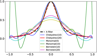
(a) A filter and its approximation results.

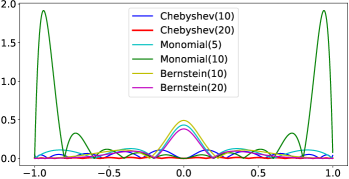
(b) The error of approximation results.

Figure 2: (a) A Runge filter $h(\hat{\lambda})=1/(1+25\hat{\lambda}^{2})$ and its approximation results by different polynomial bases. (b) The errors of the different approximation results.

4.4 Comparison of Different Polynomial Bases

We perform numerical studies comparing the Chebyshev basis to the Monomial and Bernstein bases to demonstrate ChebNetII’s approximation power. Considering a Runge filter $h(\hat{\lambda})=1/(1+25\hat{\lambda}^{2}),\hat{\lambda}\in[-1,1]$, Figures 2(a) and 2(b) depict the approximation results and errors for several polynomial bases, with the polynomial degree $K$ denoted by the numbers in brackets. We find that the Chebyshev basis has a faster convergence rate than the Bernstein basis and does not exhibit the Runge phenomenon compared to the Monomial basis. Notably, JacobiConv [40] investigated different polynomial bases at the same period and discovered that orthogonal polynomial bases could learn graph filters more effectively. These findings provide empirical motivations for designing GNNs with Chebyshev interpolation.

5 Conclusion

This paper revisits the problem of approximating spectral graph convolutions with Chebyshev polynomials. We show that ChebNet’s inferior performance is primarily due to illegal coefficients learned by approximating analytic filter functions, which leads to over-fitting. Moreover, we propose ChebNetII, a new GNN model based on Chebyshev interpolation, enhancing the original Chebyshev polynomial approximation while reducing the Runge phenomenon. Experiments show that ChebNetII outperforms SOTA methods in terms of effectiveness on real-world both homophilic and heterophilic datasets. For future work, a promising direction is further to improve the performance of ChebNetII on large graphs and investigate the scalability of spectral-based GNNs.

Appendix A Additional details for spectral-based GNNs

Vanilla GCN. [21] The vanilla GCN uses a simplified first tow Chebyshev polynomials as the graph convolution, which is a fixed low-pass filter [1, 41, 43, 54]. In particular, the vanilla GCN sets $K=1$, $w_{0}=-w_{1}=w$ and $\lambda_{max}=2$ in Equation (2) to obtain the filtering operation $\mathbf{y}=w(\mathbf{I}+\mathbf{D}^{-1/2}\mathbf{A}\mathbf{D}^{-1/2})\mathbf{x}$. The vanilla GCN proposes the renormalization trick which replaces $\mathbf{I}+\mathbf{D}^{-1/2}\mathbf{A}\mathbf{D}^{-1/2}$ by a normalized version $\tilde{\mathbf{P}}=\tilde{\mathbf{D}}^{-1/2}\tilde{\mathbf{A}}\tilde{\mathbf{D}}^{-1/2}=(\mathbf{D}+\mathbf{I})^{-1/2}(\mathbf{A}+\mathbf{I})(\mathbf{D}+\mathbf{I})^{-1/2}$. Finally, the graph convolution of each layer in the vanilla GCN is defined as

$$\mathbf{H}^{(\ell+1)}=\sigma\left(\tilde{\mathbf{P}}\mathbf{H}^{(\ell)}\mathbf{W}^{(\ell)}\right),$$ (13)

where $\sigma$ denotes the activation function, $\mathbf{H}^{(\ell)}$ is the representation of $\ell$-th each layer and $\mathbf{H}^{(0)}=\mathbf{X}$.

APPNP. [22] APPNP utilizes Personalized PageRank to derive the spectral graph convolutions. The model structure of APPNP is defined as

$$\mathbf{Y}=\sum\limits_{k=0}^{K}\alpha(1-\alpha)^{k}\tilde{\mathbf{P}}^{k}f_{\theta}(\mathbf{X}),$$ (14)

where $\alpha\in(0,1]$ denotes the teleport probability and $f_{\theta}(\cdot)$ denotes a neural network with parameters $\{\theta\}$. APPNP first decouples the feature transformation and propagation, which improves its scalability.

GPR-GNN. [6] GPR-GNN approximates spectral graph convolutions using the Monomial basis, which can also be understood as the Generalized PageRank. It has the following model structure.

$$\mathbf{Y}=\sum\limits_{k=0}^{K}w_{k}\tilde{\mathbf{P}}^{k}f_{\theta}(\mathbf{X}),$$ (15)

where $f_{\theta}(\cdot)$ denotes a neural network with parameters $\{\theta\}$. Essentially, the spectral filter of GPR-GNN is $h(\tilde{\lambda})=\sum\nolimits_{k=0}^{K}w_{k}\tilde{\lambda}^{k}$, where $\tilde{\lambda}$ denotes the eigenvalues of $\tilde{\mathbf{P}}$.

BernNet. [17] BernNet uses the Bernstein basis to approximate graph spectral filters, whose model expression is defined as

$$\mathbf{Y}=\sum\limits_{k=0}^{K}w_{k}\frac{1}{2^{K}}\binom{K}{k}(2\mathbf{I}-\mathbf{L})^{K-k}\mathbf{L}^{k}f_{\theta}\left(\mathbf{X}\right),$$ (16)

where $f_{\theta}(\cdot)$ represents a neural network like GPR-GNN and the spectral filter is $h(\lambda)=\sum\nolimits_{k=0}^{K}w_{k}\frac{1}{2^{K}}\binom{K}{k}(2-\lambda)^{K-k}\lambda^{k}$, where $\frac{1}{2^{K}}\binom{K}{k}(2-\lambda)^{K-k}\lambda^{k}$ denotes the Bernstein basis.

Appendix B Spectral Filter and Node Classification

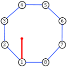
(a) Ring graph and the graph signal before filtering.

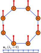
(b) Signal after impulse low-pass filter corresponds to homophilic labels.

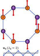
(c) Signal after impulse high-pass filter corresponds to heterophilic labels.

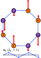
(d) Signal after impulse band-pass filter corresponds to mixed labels.

Figure 3: A ring graph and filtering results. The red bar indicates the graph signal and the blue line charts represent the eigenvectors. Node labels are represented by orange and purple colors.

In this subsection, we show why learning the right spectral filter is crucial for node classification tasks on homophilic and heterophilic graphs. Given a graph signal vector $\mathbf{x}$, the filtering operation is defined as

$$\mathbf{y}=\mathbf{U}diag\left[h(\lambda_{1}),...,h(\lambda_{n})\right]\mathbf{U}^{T}\mathbf{x},$$ (17)

where $\mathbf{y}$ denotes the filtering results of $\mathbf{x}$ and $h(\lambda)$ is the spectral filter, which is a function of eigenvalues of the Laplacian matrix $\mathbf{L}$.

Figure 3 illustrates the relationship between various filters and the homophilic/heterophilic node labels on a ring graph. Figure 3(a) shows a ring graph, the red bar indicates the one-hot graph signal $\mathbf{x}$. When we apply low/high/band-pass filters on the graph signal $\mathbf{x}$, the output $\mathbf{y}$ can be used to classify homophilic/heterophilic node labels. For example, consider the homophilic graph 3(b) where all nodes have the same orange label. If we apply an impulse low-pass filter $h(\lambda)=\delta_{0}(\lambda)$ where $\delta_{0}(\lambda)=1$ if $\lambda=0$ and $\delta_{0}(\lambda)=0$ for $\lambda>0$, then the resulting graph signal $\mathbf{y}$ corresponds to the first eigenvector of the ring graph’s Laplacian matrix. Consequently, the filtered signal evenly spreads over each node, which can be used to make perfect node classification on this homophilic graph.

On the other hand, figure 3(c) shows a heterophilic ring graph where any two connecting nodes have different labels (orange and purple). If we apply an impulse high-pass filter $h(\lambda)=\delta_{2}(\lambda)$ where $\delta_{2}(\lambda)=1$ if $\lambda=2$ and $\delta_{2}(\lambda)=0$ for $\lambda<2$, then the resulting graph signal $\mathbf{y}$ corresponds to the last eigenvector of the ring graph’s laplacian matrix. Consequently, the filtered signal exhibits alternating signs, which can be used to make perfect node classification on this heterophilic graph. Finally, figure 3(d) shows a ring graph with mixed homophilic/heterophilic node labels, which can be handled by an impulse band-pass filter $h(\lambda)=\delta_{1}(\lambda)$ where $\delta_{1}(\lambda)=1$ if $\lambda=1$ and $\delta_{1}(\lambda)=0$ otherwise.

The above example shows that the spectral filter is crucial to correct node classification on homophilic and heterophilic graphs.

Appendix C Chebyshev basis

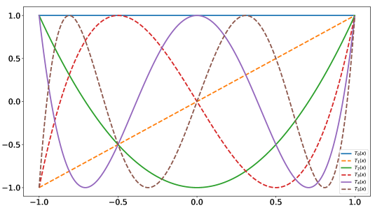
Figure 4: Chebyshev polynomials $T_{k}(x),k=0,1,2,3,4,5$.

The Chebyshev polynomials $T_{k}(x)$ for $x\in[-1,1]$ satisfy the following three-term recurrence relation.

$$T_{k}(x)=2xT_{k-1}(x)-T_{k-2}(x),k=2,3,\cdots$$

with starting values $T_{0}(x)=1,T_{1}(x)=x$. The figure 4 exhibits the first six Chebyshev polynomials. We can observe that Chebyshev polynomial $T_{k}(x)$ with larger $k$ corresponds to higher frequency oscillation, which should be constrained in the Chebyshev expansion for approximating an analytic function according to Theorem 2.1.

Appendix D More details for Polynomial Interpolation

In this subsection, we give an explicit expression of the general polynomial interpolation. The following Lemma D.1 defines the general polynomial interpolation for spectral filters.

Lemma D.1.

(Polynomial interpolation)  [27] Given a continuous filter function $h$ that is defined in $[-1,1]$, and given its values at $K+1$ points $\hat{\lambda}_{0}<\hat{\lambda}_{1}<...<\hat{\lambda}_{K}\in[-1,1]$, there exists a unique polynomial of degree smaller than or equal to $K$ such that

$$P_{K}(\hat{\lambda}_{k})=h(\hat{\lambda}_{k}),\quad P_{K}(\hat{\lambda})=\sum\limits_{k=0}^{K}a_{k}\hat{\lambda}^{k},\quad k=0,1,...,K,$$ (18)

with polynomial coefficients $a_{k}$ which can be uniquely derived by solving a Vandermonde linear system induced by equations  (18). In particular, the Vandermonde linear system is defined as

$$\begin{bmatrix}1&\hat{\lambda}_{0}&\hat{\lambda}_{0}^{2}&\cdots&\hat{\lambda}_{0}^{K}\\ 1&\hat{\lambda}_{1}&\hat{\lambda}_{1}^{2}&\cdots&\hat{\lambda}_{1}^{K}\\ \vdots&\vdots&\vdots&\vdots&\vdots\\ 1&\hat{\lambda}_{K}&\hat{\lambda}_{K}^{2}&\cdots&\hat{\lambda}_{K}^{K}\end{bmatrix}\begin{bmatrix}a_{0}\\ a_{1}\\ \vdots\\ a_{K}\end{bmatrix}=\begin{bmatrix}h(\hat{\lambda}_{0})\\ h(\hat{\lambda}_{1})\\ \vdots\\ h(\hat{\lambda}_{K})\end{bmatrix}.$$ (19)

Because solving the Equation 19 for a large number of data points is expensive, the general polynomial interpolation using the Vandermonde matrix is not feasible. As a result, Lagrange interpolation is a essentially equivalent approach to the polynomial interpolation with the Vandermonde matrix. The following Lemma D.2 defines the Lagrange interpolation.

Lemma D.2.

(Lagrange interpolation) [27] Given a continuous filter function $h$ that is defined on $[-1,1]$, and given its values at $K+1$ points $\hat{\lambda}_{0}<\hat{\lambda}_{1}<...<\hat{\lambda}_{K}\in[-1,1]$, there exists a unique polynomial of degree smaller than or equal to $K$ such that

$$P_{K}(\hat{\lambda}_{k})=h(\hat{\lambda}_{k}),\quad P_{K}(\hat{\lambda})=\sum\limits_{k=0}^{K}h(\hat{\lambda}_{k})L_{k}(\hat{\lambda}),\quad k=0,1,...,K,$$ (20)

where $L_{i}(\hat{\lambda})$ is defined by

$$L_{k}(\hat{\lambda})=\frac{\pi_{K+1}(\hat{\lambda})}{(\hat{\lambda}-\hat{\lambda}_{k})\pi^{\prime}_{K+1}(\hat{\lambda})}=\frac{\prod\nolimits_{j=0,j\neq k}^{K}(\hat{\lambda}-\hat{\lambda}_{j})}{\prod\nolimits_{j=0,j\neq k}^{K}(\hat{\lambda}_{k}-\hat{\lambda}_{j})}$$ (21)

with the nodal polynomial $\pi_{K+1}(\hat{\lambda})=\prod\nolimits_{j=0}^{K}(\hat{\lambda}-\hat{\lambda}_{j})$.

The relation of the general polynomial interpolation to Chebyshev interpolation. The general polynomial interpolation (Lemma D.1) and Lagrange interpolation (Lemma D.2) are essentially equivalent, and in practice, we generally sample $K$ points uniformly as the interpolation points. Chebyshev interpolation is distinguished by using Chebyshev Nodes (Definition 3.1) rather than equispaced interpolation points. In other words, we can define Chebyshev interpolation by replacing the equispaced interpolation points of polynomial interpolation (Lemma D.1) and Lagrange interpolation (Lemma D.2) with Chebyshev Nodes. It is worth noting that intuitively increasing the number of interpolation points should improve the approximation quality, but this is not always the case due to the Runge phenomenon[10]. Chebyshev interpolation can effectively avoid the Runge phenomenon and thus makes the error decrease as interpolation points increase (Theorem 3.3).

Appendix E Additional experimental details

Baseline Implementations. For MLP, GCN, ChebNet, AMAR and APPNP, we use the Pytorch Geometric library implementations [11]. And we use the implementation released by the authors for other baselines.

• Pytorch Geometric library: https://github.com/pyg-team/pytorch_geometric/tree/master/benchmarkhttps://github.com/pyg-team/pytorch_geometric/tree/master/benchmark

• GPR-GNN: https://github.com/jianhao2016/GPRGNNhttps://github.com/jianhao2016/GPRGNN

• BernNet: https://github.com/ivam-he/BernNethttps://github.com/ivam-he/BernNet

• GCNII: https://github.com/chennnM/GCNIIhttps://github.com/chennnM/GCNII

• TWIRLS: https://github.com/FFTYYY/TWIRLShttps://github.com/FFTYYY/TWIRLS

• EGNN: https://github.com/Kaixiong-Zhou/EGNNhttps://github.com/Kaixiong-Zhou/EGNN

• PDE-GCN: https://openreview.net/forum?id=wWtk6GxJB2xhttps://openreview.net/forum?id=wWtk6GxJB2x

• SIGN: https://github.com/twitter-research/signhttps://github.com/twitter-research/sign

• GBP: https://github.com/chennnM/GBPhttps://github.com/chennnM/GBP

• NDLS^∗: https://github.com/zwt233/NDLShttps://github.com/zwt233/NDLS

• LINK and LINKX: https://github.com/CUAI/Non-Homophily-Large-Scalehttps://github.com/CUAI/Non-Homophily-Large-Scale

E.1 Experiments in Section 2

Setting. We use three citation graphs: Cora, Citeseer, and Pubmed [35, 45]. For dataset splitting, we apply the standard fixed training/validation/testing split [45] with 20 nodes per class for training, 500 nodes for validation, and 1,000 nodes for testing. We report the mean results over 10 runs for each model.

Table 10: The number of parameters for each model on Cora.

Method	Parameters
ChebNet(2)	138.0k
ChebNet(10)	230.4k
GCN	92.1k
GPR-GNN	92.1k
BernNet	92.1k
ChabBase	92.1k

For ChebNet, we set the hidden units as 32 for the propagation steps $K=2$ and set the hidden units as 16 for the propagation steps $K=10$ and use 2 convolutional layers. For GCN, we use 2 convolutional layers with 64 hidden units. For GPR-GNN and BernNet, we use 2-layer MLP with 64 hidden units and set the propagation steps $K=10$. Following the released code, we use PPR to initialize the coefficients $w_{k}$ with $\alpha=0.1$ for GPR-GNN, and initialize $w_{k}=1.0$ for $k=0,\cdots,K$ for BernNet. For ChebBase, we also utilize 2-layer MLP with 64 hidden units and set the propagation steps $K=10$ as the same as GPR-GNN and BernNet. we set $w_{0}=1.0$, $w_{k}=0.0$ for $k\neq 0$ to initialize the Chebyshev coefficients for ChebBase, corresponding to an initial state with no feature propagation. For other hyperparameter tuning, we set the learning rate as 0.01, optimize weight decay over $\{0.0005,0.05\}$ and dropout over ${0.5,0.8}$ for all models.

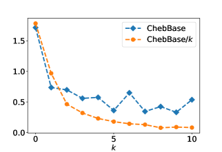
(a) Citeseer.

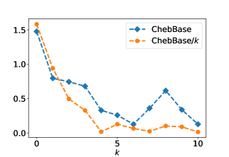
(b) Pubmed.

Figure 5: Illustrations of the Chebyshev coefficients learnt by ChebBase and ChebBase/$k$ on Citeseer and Pubmed.

Our setup ensures that each model’s parameters are as exact as possible for fairness in comparison. Table 10 displays the number of parameters for each method on the Cora dataset, with the $K$ for ChebNet indicated by the numbers in parentheses. We can observe that the number of parameters for each model is close to 100k. Note that with $K=10$, ChebNet’s hidden units are already equivalent to 16, and if we keep reducing them, the results will deteriorate.

Additional results. Figure 5 shows the absolute values of Chebyshev coefficients learnt by ChebBase and ChebBase/$k$ on Citeseer and Pubmed. We can observe that the coefficients of ChebBase/k could more readily satisfy the convergence constraint as the same as Figure 1(b), which validates Theorem 2.1.

Table 11: The hyper-parameters of baselines.

Method	Hyper-parameters
MLP	layers: 2, hidden: 64, lr:{0.01,0.05}, $L_{2}$: {0.0005,0.0}, dropout: 0.5
GCN	layers: 2, hidden: 64, lr:{0.01,0.05}, $L_{2}$: {0.0005,0.0}, dropout: 0.5
APPNP	layers: 2, hidden: 64, lr:{0.01,0.05}, $L_{2}$: {0.0005,0.0}, dropout: 0.5, $\alpha$: {0.1, 0.2, 0.5, 0.9}, $K$: 10
ARMA	layers: 2, hidden: 64, lr:{0.01,0.05}, $L_{2}$: {0.0005,0.0}, stacks: 2, ARMA_layers: 1, skip_dropout: {0.25,0.75}, dropout: 0.5
ChebNet	layers: 2, hidden: 32, lr:{0.01,0.05}, $L_{2}$: {0.0005,0.0}, $K$: 2, dropout: 0.5
GPRGNN	layers: 2, hidden: 64, $K$: 10, lrl:{0.01,0.05}, lrp: {0.01,0.05}, $\alpha$: {0.1, 0.2, 0.5, 0.9}, dropoutl: 0.5, dropoutp: {0.0,0.5,0.7}, $L_{2}$: {0.0005,0.0}
BernNet	layers: 2, hidden: 64, $K$: 10, lrl:{0.01,0.05}, lrp: {0.001,0.002,0.01,0.05}, dropoutl: 0.5, dropoutp: {0.0,0.5,0.6,0.7,0.9}, $L_{2}$: {0.0005,0.0}

Table 12: The hyper-parameters of ChebNetII for semi-supervised learning.

Dataset	layer	hidden	$K$	lrl	$L_{2_{l}}$	dropoutl	lrp	$L_{2_{p}}$	dropoutp
Cora	2	64	10	0.01	0.0005	0.5	0.001	0.05	0.8
Citeseer	2	64	10	0.01	0.0005	0.5	0.001	0.05	0.8
Pubmed	2	64	10	0.01	0.0005	0.5	0.005	0.05	0.5
Chameleon	2	64	10	0.01	0.0005	0.5	0.0005	0.0	0.5
Squirrel	2	64	10	0.01	0.0005	0.5	0.0005	0.0	0.5
Actor	2	64	10	0.01	0.0005	0.5	0.01	0.0005	0.6
Texas	2	64	10	0.01	0.0005	0.8	0.001	0.0	0.7
Cornell	2	64	10	0.01	0.0005	0.8	0.001	0.0005	0.7

E.2 Semi-supervised node classification with polynomial based methods

Setting. For the baselines, we follow their papers’ settings and list the hyper-parameters in Table 11, where lr represents the learning rate and $L_{2}$ denotes the weight decay. For ARMA, we set the number of parallel stacks as 2, use 1 ARMA layer and optimize the dropout probability of the skip connection over $\{0.25,0.75\}$, following the paper  [2]. For GPR-GNN and BernNet, we use lr_l, $L_{2_{l}}$ and dropout_l to denote the learning rate, weight decay and dropout for the linear layer, respectively, and use lr_p, $L_{2_{p}}$ and dropout_p for the propagation layer. We optimize these parameters according to the reports in their paper [6, 17].

For ChebNetII, we use a 2-layers MLP with 64 hidden units for linear layer as the same as GPR-GNN and BernNet. Our setup ensures that each model’s parameters are as exact as possible for fairness in comparison. We optimize the hyper-parameters for the linear and propagation layers, respectively. Table 12 displays the hyper-parameters of ChebNetII for the semi-supervised node classification task.

Results of fixed splits. Table 13 exhibits the results of the semi-supervised node classification with fixed splits. We can observe that ChebNetII performs nearly identically to the results with random splits (Table 6), achieving the best performance in seven of the eight datasets, demonstrating the Chebyshev basis’s superior expression power.

Table 13: Mean classification accuracy of semi-supervised node classification with fixed splits.

Method	Cham.	Squi.	Texas	Corn.	Actor	Cora	Cite.	Pubm.
MLP	21.91${}_{\pm\text{2.11}}$	23.42${}_{\pm\text{0.94}}$	45.03${}_{\pm\text{2.45}}$	46.18${}_{\pm\text{5.10}}$	29.16${}_{\pm\text{0.52}}$	58.88${}_{\pm\text{0.62}}$	56.97${}_{\pm\text{0.54}}$	73.15${}_{\pm\text{0.28}}$
GCN	39.14${}_{\pm\text{0.60}}$	30.06${}_{\pm\text{0.75}}$	32.42${}_{\pm\text{2.23}}$	35.57${}_{\pm\text{3.55}}$	21.96${}_{\pm\text{0.54}}$	81.32${}_{\pm\text{0.18}}$	71.77${}_{\pm\text{0.21}}$	79.15${}_{\pm\text{0.18}}$
ChebNet	31.27${}_{\pm\text{1.34}}$	28.37${}_{\pm\text{0.28}}$	28.55${}_{\pm\text{3.28}}$	25.54${}_{\pm\text{3.42}}$	26.13${}_{\pm\text{1.27}}$	80.54${}_{\pm\text{0.38}}$	70.35${}_{\pm\text{0.33}}$	75.52${}_{\pm\text{0.75}}$
ARMA	40.58${}_{\pm\text{0.67}}$	28.45${}_{\pm\text{0.55}}$	47.84${}_{\pm\text{3.35}}$	30.89${}_{\pm\text{4.23}}$	27.26${}_{\pm\text{0.32}}$	83.15${}_{\pm\text{0.54}}$	71.41${}_{\pm\text{0.36}}$	78.75${}_{\pm\text{0.14}}$
APPNP	30.06${}_{\pm\text{0.96}}$	25.18${}_{\pm\text{0.35}}$	46.31${}_{\pm\text{3.01}}$	45.73${}_{\pm\text{4.85}}$	28.19${}_{\pm\text{0.31}}$	83.52${}_{\pm\text{0.24}}$	72.09${}_{\pm\text{0.25}}$	80.23${}_{\pm\text{0.15}}$
GPR-GNN	30.56${}_{\pm\text{0.94}}$	25.11${}_{\pm\text{0.51}}$	45.76${}_{\pm\text{3.78}}$	43.42${}_{\pm\text{4.95}}$	27.32${}_{\pm\text{0.83}}$	83.95${}_{\pm\textbf{0.22}}$	70.92${}_{\pm\text{0.57}}$	78.97${}_{\pm\text{0.27}}$
BernNet	26.35${}_{\pm\text{1.04}}$	24.57${}_{\pm\text{0.72}}$	48.21${}_{\pm\text{3.17}}$	46.64${}_{\pm\text{5.62}}$	29.27${}_{\pm\text{0.23}}$	83.15${}_{\pm\text{0.32}}$	72.24${}_{\pm\text{0.25}}$	79.65${}_{\pm\text{0.25}}$
ChebNetII	46.45${}_{\pm\textbf{0.53}}$	36.18${}_{\pm\textbf{0.46}}$	54.68${}_{\pm\textbf{3.87}}$	50.92${}_{\pm\textbf{5.49}}$	29.54${}_{\pm\textbf{0.46}}$	83.67${}_{\pm\text{0.33}}$	72.75${}_{\pm\textbf{0.16}}$	80.48${}_{\pm\textbf{0.23}}$

E.3 Full-supervised node classification

We use the same model settings for the baselines in the semi-supervised node classification task and perform a grid search to tune their hyper-parameters. For GCNII [5], TWIRLS [44], EGNN [51] and PDE-GCN [9], we use the experimental settings and hyper-parameters reported in their papers for the full-supervised task.

For ChebnetII, we use Equation (8) as the propagation process and use a 2-layers MLP with 64 hidden units for all datasets. We optimize the hyper-parameters for the linear and propagation layers, respectively. Table 14 exhibits the hyper-parameters of ChebNetII for the full-supervised tasks.

Table 14: The hyper-parameters of ChebNetII for full-supervised learning.

Dataset	layer	hidden	$K$	lrl	$L_{2_{l}}$	dropoutl	lrp	$L_{2_{p}}$	dropoutp
Cora	2	64	10	0.01	0.0005	0.5	0.01	0.0005	0.0
Citeseer	2	64	10	0.01	0.0005	0.5	0.01	0.0005	0.0
Pubmed	2	64	10	0.01	0.0	0.5	0.01	0.0	0.0
Chameleon	2	64	10	0.05	0.0	0.5	0.01	0.0	0.6
Squirrel	2	64	10	0.05	0.0	0.5	0.01	0.0	0.5
Actor	2	64	10	0.05	0.0	0.5	0.01	0.0	0.9
Texas	2	64	10	0.05	0.0005	0.6	0.001	0.0	0.5
Cornell	2	64	10	0.05	0.0005	0.5	0.001	0.0005	0.6

E.4 Scalability of ChebNetII

For large heterophilic graphs, we follow the experimental setting in [25] and run each method on the same five random 50/25/25 train/val/test splits for each dataset. We use the accuracy metric for most datasets, while the ROC AUC is for genius. We utilize the published baseline results in [25], excluding GPR-GNN. For ChebNetII, we use Equation (12) as the propagation process on pokec and wiki and Equation (8) on the four remaining datasets. We achieve optimal performance by hyper-parameter grid search reported in the papers for GPR-GNN and BernNet. For ChebNetII, we also tune the hyper-parameters based on the results of the validation set. Detailed hyper-parameter settings are available in the code repository.

For OGB datasets, we use the settings and hyper-parameters reported in the baseline papers. For ChebNetII, we use Equation (12) as the propagation process and pre-compute $T_{k}(\hat{\mathbf{L}})\mathbf{X}$ for $k=0,\cdots,K$ with $K=10$. Table 15 shows the hyper-parameters of ChebNetII for OGB datasets.

Table 15: The hyper-parameters of ChebNetII for OGB datasets.

Dataset	layer	hidden	$K$	lrl	$L_{2_{l}}$	dropoutl	lrp	$L_{2_{p}}$	dropoutp
ogbn-arxiv	3	512	10	0.0005	0.0	0.5	0.01	0.0	0.0
ogbn-papers100M	3	2048	10	0.001	0.0	0.5	0.01	0.00005	0.0

Appendix F The filters learned by ChebNetII

Figure 6 reports the filter responses (where $\lambda$ denotes the eigenvalues of the normalized Laplacian matrix $\mathbf{L}$) learned by ChebNetII and BernNet on real-world datasets for the full-supervised node classification task. We observe that ChebNetII and BernNet both learn comb-alike filters on Chameleon and Squirrel, band-rejection pass filters on Texas, and low-pass filters on Citeseer. Notably, the shape of the filter learned by ChebNetII is relatively more complex, demonstrating that ChebNetII has a stronger approximating ability for learning filters.

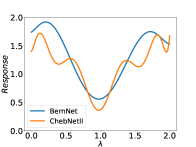
(a) Chameleon

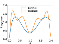
(b) Squirrel

(c) Texas

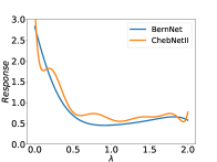
(d) Citeseer

Figure 6: Filters learnt by BernNet and ChebNetII on real-word datasets.

References

- [1] Muhammet Balcilar, Pierre Héroux, Benoit Gaüzère, Sébastien Adam, and Paul Honeine. Analyzing the expressive power of graph neural networks in a spectral perspective. In ICLR, 2021.
- [2] Filippo Maria Bianchi, Daniele Grattarola, Lorenzo Livi, and Cesare Alippi. Graph neural networks with convolutional arma filters. TPAMI, 2021.
- [3] Toon Bogaerts, Antonio D Masegosa, Juan S Angarita-Zapata, Enrique Onieva, and Peter Hellinckx. A graph cnn-lstm neural network for short and long-term traffic forecasting based on trajectory data. Transportation Research Part C: Emerging Technologies, 2020.
- [4] Ming Chen, Zhewei Wei, Bolin Ding, Yaliang Li, Ye Yuan, Xiaoyong Du, and Ji-Rong Wen. Scalable graph neural networks via bidirectional propagation. NeurIPS, 2020.
- [5] Ming Chen, Zhewei Wei, Zengfeng Huang, Bolin Ding, and Yaliang Li. Simple and deep graph convolutional networks. In ICML, pages 1725–1735. PMLR, 2020.
- [6] Eli Chien, Jianhao Peng, Pan Li, and Olgica Milenkovic. Adaptive universal generalized pagerank graph neural network. In ICLR, 2021.
- [7] Zhiyong Cui, Kristian Henrickson, Ruimin Ke, and Yinhai Wang. Traffic graph convolutional recurrent neural network: A deep learning framework for network-scale traffic learning and forecasting. T-ITS, 21(11):4883–4894, 2019.
- [8] Michaël Defferrard, Xavier Bresson, and Pierre Vandergheynst. Convolutional neural networks on graphs with fast localized spectral filtering. In NeurIPS, pages 3844–3852, 2016.
- [9] Moshe Eliasof, Eldad Haber, and Eran Treister. Pde-gcn: Novel architectures for graph neural networks motivated by partial differential equations. In NeurIPS, volume 34, 2021.
- [10] James F Epperson. On the runge example. The American Mathematical Monthly, 94(4):329–341, 1987.
- [11] Matthias Fey and Jan Eric Lenssen. Fast graph representation learning with pytorch geometric. In ICLR, 2019.
- [12] Johannes Gasteiger, Stefan Weiß enberger, and Stephan Günnemann. Diffusion improves graph learning. In NeurIPS, 2019.
- [13] Keith O Geddes. Near-minimax polynomial approximation in an elliptical region. SIAM Journal on Numerical Analysis, 15(6):1225–1233, 1978.
- [14] Amparo Gil, Javier Segura, and Nico M Temme. Numerical methods for special functions. SIAM, 2007.
- [15] William L Hamilton, Rex Ying, and Jure Leskovec. Inductive representation learning on large graphs. In NeurIPS, pages 1025–1035, 2017.
- [16] David K Hammond, Pierre Vandergheynst, and Rémi Gribonval. Wavelets on graphs via spectral graph theory. Applied and Computational Harmonic Analysis, 30(2):129–150, 2011.
- [17] Mingguo He, Zhewei Wei, Zengfeng Huang, and Hongteng Xu. Bernnet: Learning arbitrary graph spectral filters via bernstein approximation. In NeurIPS, 2021.
- [18] Weihua Hu, Matthias Fey, Marinka Zitnik, Yuxiao Dong, Hongyu Ren, Bowen Liu, Michele Catasta, and Jure Leskovec. Open graph benchmark: Datasets for machine learning on graphs. In NeurIPS, volume 33, 2020.
- [19] Dejun Jiang, Zhenxing Wu, Chang-Yu Hsieh, Guangyong Chen, Ben Liao, Zhe Wang, Chao Shen, Dongsheng Cao, Jian Wu, and Tingjun Hou. Could graph neural networks learn better molecular representation for drug discovery? a comparison study of descriptor-based and graph-based models. Journal of cheminformatics, 13(1):1–23, 2021.
- [20] Diederik P Kingma and Jimmy Ba. Adam: A method for stochastic optimization. In ICLR, 2015.
- [21] Thomas N Kipf and Max Welling. Semi-supervised classification with graph convolutional networks. In ICLR, 2017.
- [22] Johannes Klicpera, Aleksandar Bojchevski, and Stephan Günnemann. Predict then propagate: Graph neural networks meet personalized pagerank. In ICLR, 2019.
- [23] Ron Levie, Federico Monti, Xavier Bresson, and Michael M Bronstein. Cayleynets: Graph convolutional neural networks with complex rational spectral filters. Transactions on Signal Processing, 67(1):97–109, 2018.
- [24] Chang Li and Dan Goldwasser. Encoding social information with graph convolutional networks forpolitical perspective detection in news media. In ACL, 2019.
- [25] Derek Lim, Felix Hohne, Xiuyu Li, Sijia Linda Huang, Vaishnavi Gupta, Omkar Bhalerao, and Ser Nam Lim. Large scale learning on non-homophilous graphs: New benchmarks and strong simple methods. In NeurIPS, 2021.
- [26] Tanwi Mallick, Prasanna Balaprakash, Eric Rask, and Jane Macfarlane. Transfer learning with graph neural networks for short-term highway traffic forecasting. In ICPR, pages 10367–10374. IEEE, 2021.
- [27] John C Mason and David C Handscomb. Chebyshev polynomials. CRC press, 2002.
- [28] Sunil K Narang, Akshay Gadde, and Antonio Ortega. Signal processing techniques for interpolation in graph structured data. In ICASSP. IEEE, 2013.
- [29] Andrea Pallini. Bernstein-type approximations of smooth functions. Statistica, 65(2):169–191, 2005.
- [30] Hongbin Pei, Bingzhe Wei, Kevin Chen-Chuan Chang, Yu Lei, and Bo Yang. Geom-gcn: Geometric graph convolutional networks. In ICLR, 2020.
- [31] Jiezhong Qiu, Jian Tang, Hao Ma, Yuxiao Dong, Kuansan Wang, and Jie Tang. Deepinf: Social influence prediction with deep learning. In KDD, 2018.
- [32] Prakash Chandra Rathi, R Frederick Ludlow, and Marcel L Verdonk. Practical high-quality electrostatic potential surfaces for drug discovery using a graph-convolutional deep neural network. Journal of medicinal chemistry, 63(16):8778–8790, 2019.
- [33] Emanuele Rossi, Fabrizio Frasca, Ben Chamberlain, Davide Eynard, Michael Bronstein, and Federico Monti. Sign: Scalable inception graph neural networks. arXiv preprint arXiv:2004.11198, 2020.
- [34] Benedek Rozemberczki, Carl Allen, and Rik Sarkar. Multi-scale attributed node embedding. Journal of Complex Networks, 9(2):cnab014, 2021.
- [35] Prithviraj Sen, Galileo Namata, Mustafa Bilgic, Lise Getoor, Brian Galligher, and Tina Eliassi-Rad. Collective classification in network data. AI magazine, 29(3):93–93, 2008.
- [36] David I Shuman, Pierre Vandergheynst, and Pascal Frossard. Chebyshev polynomial approximation for distributed signal processing. In DCOSS, pages 1–8. IEEE, 2011.
- [37] Ljubisa Stankovic, Danilo Mandic, Milos Dakovic, Milos Brajovic, Bruno Scalzo, and Anthony G Constantinides. Graph signal processing–part ii: Processing and analyzing signals on graphs. arXiv preprint arXiv:1909.10325, 2019.
- [38] Peihao Tong, Qifan Zhang, and Junjie Yao. Leveraging domain context for question answering over knowledge graph. Data Science and Engineering, 4(4):323–335, 2019.
- [39] Petar Veličković, Guillem Cucurull, Arantxa Casanova, Adriana Romero, Pietro Lio, and Yoshua Bengio. Graph attention networks. In ICLR, 2018.
- [40] Xiyuan Wang and Muhan Zhang. How powerful are spectral graph neural networks. In ICML, 2022.
- [41] Felix Wu, Amauri Souza, Tianyi Zhang, Christopher Fifty, Tao Yu, and Kilian Weinberger. Simplifying graph convolutional networks. In ICML, 2019.
- [42] Shu Wu, Yuyuan Tang, Yanqiao Zhu, Liang Wang, Xing Xie, and Tieniu Tan. Session-based recommendation with graph neural networks. In AAAI, 2019.
- [43] Bingbing Xu, Huawei Shen, Qi Cao, Keting Cen, and Xueqi Cheng. Graph convolutional networks using heat kernel for semi-supervised learning. In IJCAI, 2019.
- [44] Yongyi Yang, Tang Liu, Yangkun Wang, Jinjing Zhou, Quan Gan, Zhewei Wei, Zheng Zhang, Zengfeng Huang, and David Wipf. Graph neural networks inspired by classical iterative algorithms. In ICML, 2021.
- [45] Zhilin Yang, William Cohen, and Ruslan Salakhudinov. Revisiting semi-supervised learning with graph embeddings. In ICML, pages 40–48. PMLR, 2016.
- [46] Rex Ying, Ruining He, Kaifeng Chen, Pong Eksombatchai, William L Hamilton, and Jure Leskovec. Graph convolutional neural networks for web-scale recommender systems. In KDD, 2018.
- [47] Wentao Zhang, Mingyu Yang, Zeang Sheng, Yang Li, Wen Ouyang, Yangyu Tao, Zhi Yang, and Bin Cui. Node dependent local smoothing for scalable graph learning. In NeurIPS, volume 34, 2021.
- [48] Xiaolong Zhang and John P. Boyd. Asymptotic coefficients and errors for chebyshev polynomial approximations with weak endpoint singularities: Effects of different bases. Science China Mathematics, 2022.
- [49] Tianyi Zhao, Yang Hu, Linda R Valsdottir, Tianyi Zang, and Jiajie Peng. Identifying drug–target interactions based on graph convolutional network and deep neural network. Briefings in bioinformatics, 22(2):2141–2150, 2021.
- [50] Elena Zheleva and Lise Getoor. To join or not to join: the illusion of privacy in social networks with mixed public and private user profiles. In Proceedings of the 18th international conference on World wide web, pages 531–540, 2009.
- [51] Kaixiong Zhou, Xiao Huang, Daochen Zha, Rui Chen, Li Li, Soo-Hyun Choi, and Xia Hu. Dirichlet energy constrained learning for deep graph neural networks. In NeurIPS, volume 34, 2021.
- [52] Hao Zhu and Piotr Koniusz. Simple spectral graph convolution. In ICLR, 2021.
- [53] Jiong Zhu, Yujun Yan, Lingxiao Zhao, Mark Heimann, Leman Akoglu, and Danai Koutra. Beyond homophily in graph neural networks: Current limitations and effective designs. In NeurIPS, 2020.
- [54] Meiqi Zhu, Xiao Wang, Chuan Shi, Houye Ji, and Peng Cui. Interpreting and unifying graph neural networks with an optimization framework. In WWW, 2021.