Four Geometry Problems to Introduce Automated Deduction in Secondary Schools

Abstract

The introduction of automated deduction systems in secondary schools face several bottlenecks, the absence of the subject of rigorous mathematical demonstrations in the curricula, the lack of knowledge by the teachers about the subject and the difficulty of tackling the task by automatic means.

Despite those difficulties we claim that the subject of automated deduction in geometry can be introduced, by addressing it in particular cases: simple to manipulate by students and teachers and reasonably easy to be dealt by automatic deduction tools.

The subject is discussed by addressing four secondary schools geometry problems: their rigorous proofs, visual proofs, numeric proofs, algebraic formal proofs, synthetic formal proofs, or the lack of them. For these problems we discuss a lesson plan to address them with the help of Information and Communications Technology, more specifically, automated deduction tools.

1 Introduction

The introduction of automated deduction systems in secondary schools face several bottlenecks, the absence of the subject, rigorous mathematical demonstrations, not to mention formal proofs, in many of the national curricula, the lack of knowledge (and/or training) by the teachers about the subject [25] and the difficulty of tackling the task by automatic means [4], are the most important in our opinion.

In the area of geometry there are now a large number of computational tools that can be used to perform many different tasks, dynamic geometry systems (DGS), computer algebra systems (CAS), geometry automatic theorem provers (GATP) among others [22]. These tools can be useful to address the subject of proofs in secondary schools.

The subject of automated deduction has been progressing for many years now and has already attained some remarkable progresses, but there are many obstacles still to be addressed when we speak about the use of geometry automated theorem provers (GATP) in secondary school classes: many of the GATP were specified and implemented for research purposes and their use and outputs are designed to be understood by experts, not for a secondary teacher/student; some of the methods (e.g. the algebraic methods) do not produce a geometric proofs; many (if not all) of the synthetic methods produce a proof, but in an axiomatic system different from the usually used by the secondary teachers/students; many of the proposed problems, e.g. those involving inequalities, are still not addressed by the GATP; in many cases the time needed for a GATP to produce an answer is to long to be useful in a classroom scenario; last (but not the least), are formal proofs what a secondary teacher/student need?

An answer to this last question is being given by interactive, tutorial, deduction systems. From the secondary schools point of view, a generic fully automated theorem prover may not be the most appropriated choice, a tutorial system, with a minimum set of rules may be a better choice. What is needed is a system that allows the students to make conjectures and proofs, in natural language and with a set of rules, the closest possible with their usual practice. The tutorial systems are much close to provide such approach then the generic automated theorem provers.

Overview of the paper. The paper is organised as follows: first, in Section 2,  four secondary school geometry problems are introduced and the development of proofs with the help of Information and Communications Technology (ICT) tools, is discussed. In Section 3 the case for a new approach, a tailored, to the needs of secondary schools, axiom system approach is discussed. In Section 4 final conclusions are drawn. In appendix A a lesson plan for a classroom, where automated deduction tools could be introduced, is given and finally in appendix B the details of the use of the ICT tools for the problem 1 are shown.

2 Use of GATP in Secondary Schools

In the recent book edited by Gila Hanna, David Reid, and Michael de Villiers, Proof Technology in Mathematics Research and Teaching [10] many issues related to the use of automated deduction methods and tools are discussed. In its four parts: Strengths and limitations of automatic theorem provers; Theoretical perspectives on computer-assisted proving; Suggestions for the use of proof software in the classroom; Classroom experience with proof software, we have a comprehensive coverage of the area. The present study it is intended as a new contribution to the area, in a more hands-on approach.

In appendix A a lesson plan for the study of the proofs in geometry is presented and in the following sections, four problems, that could be the subject of the lesson plan, are presented and the use of ICT tools for the development of their formal proofs is discussed. For each of these problems its adequacy for the intended goal is discussed.

2.1 Dynamic Geometry and Automated Deduction Tools

Dynamic geometry systems and geometry automated theorem provers are tools that enable teachers and students to explore existing knowledge, to create new constructions and conjecture new properties. Dynamic geometry systems allow building geometric constructions from free objects and elementary constructions, it is possible to manipulate the free objects (objects universally quantified), preserving the geometric properties of the constructions. Moving the free points, on the one hand, we can conjecture that a given property is true. Although those manipulations are not formal proofs because only a finite set of positions are being considered and because visualisation can be misleading, they provide a first clue to the truthfulness of a given geometric conjecture. On the other hand, geometry automated theorem provers allow the development of formal proofs. Based on different approaches (e.g. algebraic, synthetic) they allow its users to check the soundness of a construction and also, in some cases, to create formal proofs for a given geometric conjectures.

In the following we focus on some ICT tools that can be used to help students and teachers in the exploration of geometric proofs. GeoGebra is a very well-known DGS, but it also contains several GATP that can be used under a portfolio strategy [3, 13, 14, 19]. Java Geometry Expert (JGEX), a GATP and DGS combo with a strong focus on the formal proofs engines: the Wu, Gröbner bases, area, full-angle and deductive database methods. It is possible to add a conjecture to a given geometric construction and ask for its proof with natural and visual language renderings [28]. Geometry Constructions $\rightarrow$ LaTeX Converter (GCLC), a GATP, with a graphics engine, for the Wu, Gröbner bases and area methods. It is possible to add a conjecture to a given geometric construction (with a graphical rendering) and ask for its proof with natural language rendering [11, 12]. Prover 9 is a generic automated theorem prover for first-order and equational logic. It is not specific to geometry, but can be used in geometry, provided a specific set of axioms (e.g. Tarski, Full-angle [6, 21]), is given.

2.2 The Four Geometric Problems

Using a DGS (GeoGebra, JGEX) it is always possible to dynamically manipulate the geometric construction, getting a visual check for the conjecture at hand. Both programs also allow to perform a numerical check. In either cases we have checks, not proofs. For the next step we need a GATP (incorporated in the DGS or not) or a generic ATP (e.g. Prover9).

The GATP came in different forms, algebraic (GeoGebra, GCLC, JGEX), synthetic: by a geometric proof method (GCLC, JGEX); or by a logical proof method (Prover9).

The algebraic provers (Wu’s method, Gröbner Basis method, etc.) are not that useful in the secondary classroom. Most of the times the output of a formal proof is only a yes/no answer, even when a proof script is produced, it is too complex and not related with geometric reasoning, to be used in a secondary classroom.

The geometric provers (area method, full-angle method, database method, etc.) provide a geometric proof script, readable, but based in axiomatic systems that are not the usually used in secondary classrooms (see Appendix B), so its usefulness is diminished by that fact.

JGEX has a very interesting feature, it links the formal proof with the geometric construction with visual elements (colours, blinking effects, etc.). It is not being developed at this moment, but given that the code is now open source, available at GitHub, maybe its development can be resumed in the future.

Generic ATP, like Prover9, using an axiomatic system for geometry, can also be used, the proof is done by refutation using the resolution method, so it can be used by teachers (maybe with the help of an expert) as a guide to construct a formal proof, to be rendered during a class, to the students.

Problem 1

Theorem.

Show that for any given convex quadrilateral, $[ABCD]$, that $[EFGH]$, where each of the points is the mid point of a segment in $[ABCD]$, is a parallelogram.

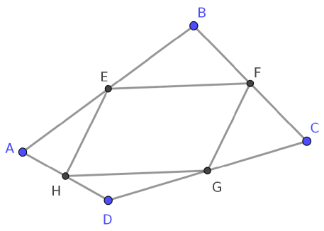
Figure 1: Problem 1

Proof.

Consider any convex quadrilateral $[ABCD]$, as shown in figure 1 where $E$, $F$, $G$ and $H$ are the midpoints of $[AB]$, $[BC]$, $[CD]$ and $[DA]$ respectively. Draw the diagonal $[AC]$ (see Figure 2), so the triangles $\Delta ABC$ and $\Delta EBF$ are similar since they have a common angle, $\alpha=\angle ABC$, and from one to the other the two pairs of sides $[AB]$, $[EB]$ and $[BC]$, $[FB]$ (which are contained on the sides of the angle) are directly proportional, $\frac{|AB|}{|EB|}=\frac{|CB|}{|FB|}$ (Side-Angle-Side case).

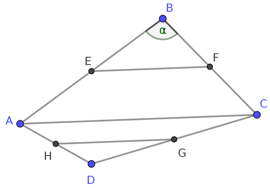
Figure 2: Sides $[EF]$ and $[HG]$ are parallel

Given that, the angles $\angle BAC$ and $\angle BEF$ are congruent and as these angles have a common side, then $[EF]\|[AC]$.

Following an analogous reasoning, we have that $[AC]\|[GH]$, since the triangles $\Delta DHG$ and $\Delta DAC$ are similar.

We have that $[EF]\|[AC]$ and $[AC]\|[GH]$ then by the transitive property of the parallelism relationship it can be concluded that $[EF]\|[GH]$.

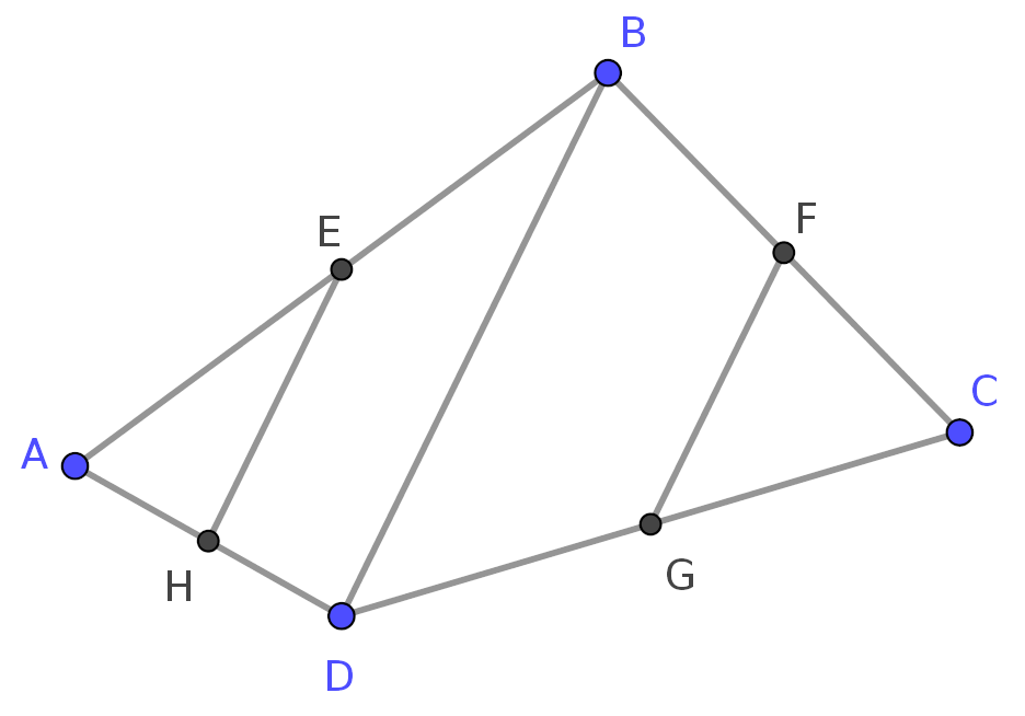
Figure 3: Sides $[FG]$ and $[EH]$ are parallel

Draw the diagonal $[BD]$ (see Figure 3). Following a reasoning similar to the previous step it can be proved that $[FG]\|[EH]$.

Since $[EF]\|[GH]$ and $[EH]\|[FG]$ it can be concluded that, the vertices of the midpoints of any quadrilateral convex are vertices of a parallelogram. ∎

Formal proofs, done with the help of ICT tools:

GeoGebra

visual dynamic and numerical checks. A formal (algebraic) proof is possible, via the Prove or ProveDetails commands, with a yes/no answer.

JGEX

visual dynamic and numerical checks. Geometry deductive database method; full-angle method; Gröbner bases method; Wu’s method (less than 1 second) — formal proofs with visual helps.

GCLC

area method, 0.001 seconds; Wu’s method, 0.051 seconds; Gröbner bases method 0.132 seconds — with formal proof scripts.

Prove9

geometry deductive database axioms, resolution method 0.02 seconds — formal proof script.

For this problem we have an array of choices, the GeoGebra and the JGEX tools are the most complete: DGS; checks; formal proofs, in one single package. JGEX provides proof scripts and visual aids. GeoGebra is the best known by teachers and students. GCLC can also be considered, although it lacks the dynamic aspect and the area method is based on an axiom system different from the usual used in secondary schools. Prover9, with a proper axiom system for geometry, is capable of develop formal proofs, producing a readable proof script. But it is a technical tool, only usable by experts. In appendix B the proofs done by the different ICT tools are given in more detail.

Problem 2

Theorem.

Consider the convex quadrilateral $[ABCD]$, like the one represented in the figure 4, Assuming that $|BD|>|BC|$ and that $\alpha=\angle CAB>\angle ABC=\beta$, show that $|BD|>|AC|$.

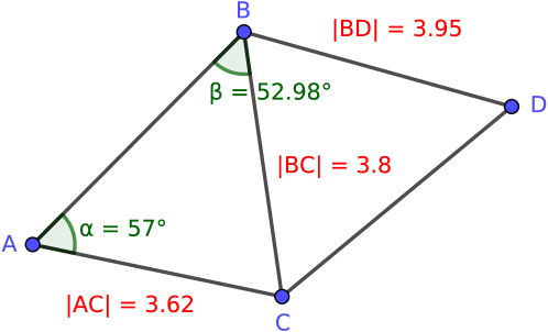
Figure 4: Problem 2

Proof.

Given that in any triangle, the angle with the greatest amplitude is opposed to the side with the longest length, we have that in the $\Delta ABC$, $|BC|>|AC|$.

Given that $|BD|>|BC|$, by hypothesis and, $|BC|>|AC|$, just proved above, due to the transitive property of the ’$>$’ order relation of we have $|BD|>|AC|$. ∎

Proofs with the help of ICT tools:

GeoGebra

visual dynamic and numerical checks. Using GeoGebra’s new tool, Discover, it is possible a formal proof, but without a proof script.

JGEX

visual dynamic and numerical checks.

The different formal proving approaches are not possible (apart the new algebraic approach built-in in GeoGebra) given that the current axiomatic systems/methods do not deal with inequalities.

Problem 3

Theorem.

Knowing that $BC\|FG$, $|BC|=|CD|$ and $BD\|EF$ (see Fig. 5), show that $G$ is equidistant from $E$ and $F$.

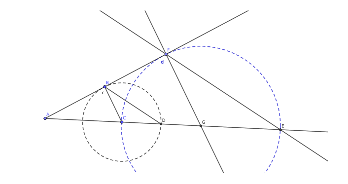
Figure 5: Problem 3

Proof.

$\angle BDC\cong\angle FEG$, since they are corresponding angles of two parallel lines ($BD\|EF)$ crossed by another line ($AE$).

Similarly $\angle FGE\cong\angle BCD$, since they are corresponding angles of two parallel lines ($BC\|FG)$ crossed by another line ($AE$).

Given that, $\Delta[BCD]$ e $\Delta[FGE]$ are similar (case angle-angle). In this way, we have:

$$\frac{|FG|}{|BC|}=\frac{|EG|}{|CD|}$$ (1)

Since $C$ is equidistant from $B$ and $D$ we have that $|BC|=|CD|$, from this and equation 1, it can be concluded that $|FG|=|EG|$, so $G$ is equidistant from $E$ and $F$. ∎

Proofs with the help of ICT tools:

GeoGebra

visual dynamic and numerical checks. No formal proof given that the Prove command do not have the equal length conjecture.

JGEX

visual dynamic and numerical checks. Geometry deductive database method, full-angle method; Wu’s method; Gröbner basis method (less than 1 second) — formal proofs with visual helps.

GCLC

area method, not proved (time limit); Wu’s method, 0.005; Gröbner basis method, 0.005.

Prove9

geometry deductive database axioms, resolution method 0.04 seconds — formal proof script.

Again, an array of choices, the JGEX tool is the most complete: DGS; checks; formal proofs, in one single package. JGEX provides proof scripts and visual aids.

Problem 4

Theorem.

Show that the sum of the amplitudes of the internal angles of a triangle is $180^{\mathrm{o}}$.

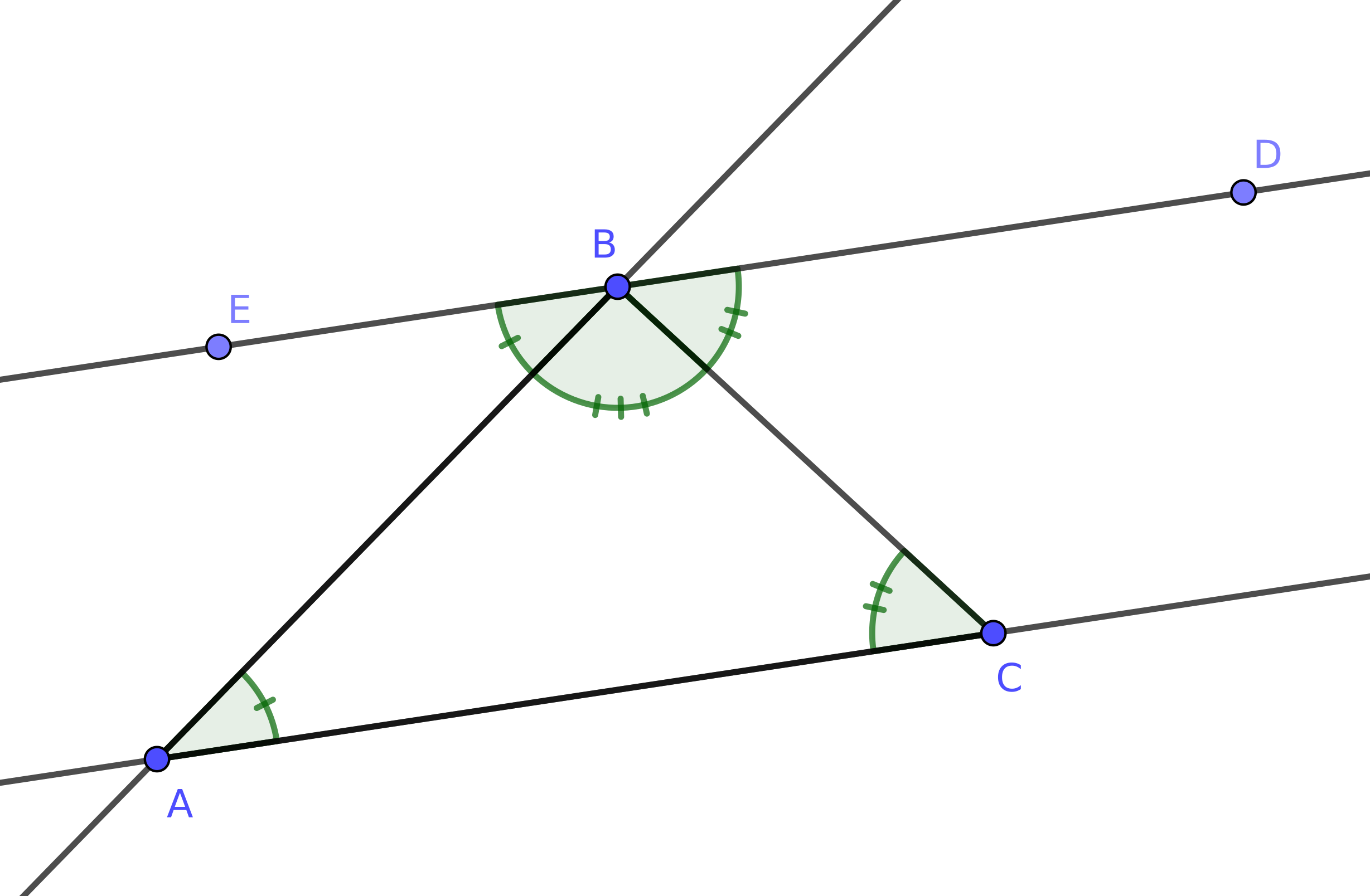
Figure 6: Problem 4

Proof.

A line is drawn parallel to $AC$ and containing the vertex $B$. Let $D$ and $E$ be two points in that line. $\angle BAC\cong\angle EBA$ given that they are alternate angles. Similarly $\angle BCA\cong\angle CBD$. The sum of the amplitudes of the $\angle CBD$, $\angle CBA$ and $\angle ABE$ angles is $180^{\mathrm{o}}$.

Thus, the sum of the interior angles of a triangle is $180^{\mathrm{o}}$. ∎

Proofs with the help of ICT tools:

GeoGebra

visual dynamic and numerical checks.

JGEX

visual dynamic and numerical checks.

The different formal proving approaches are not possible given that the current axiomatic systems and/or methods do not deal with the sum of angles.

3 A Tailored Axiom System Approach

It seems that, more than a generic (research) tool that can prove everything (or try to), a rule based approach will be more appropriate. Rule based approaches explore the possibility of building a sound, not necessarily complete, axiom system. The idea is to have a minimal set of axioms, lemmas, and rules of inference that can characterize a given sub-area of geometry. This approach has already been tried in tutorial systems like the QED-Tutrix [8] and iGeoTutor [27]. For the goal of introducing automated deduction in secondary schools, it seems the appropriated approach to pursue.

3.1 Deductive Databases in Geometry

A deductive database is a database in which new facts may be derived from facts that were explicitly introduced [9]. In a deductive database the elementary facts (axioms and lemmas) are facts in the database and each n-ary predicate is associated with a n-dimensional relation. A data-based search strategy is usually used, that is, from the old facts, new facts are deduced.

When considering the geometry deductive database method, the initial construction is used to set the initial new-fact-list, and all the axioms and lemmas are converted in tables and relations. The proof will cycle, deriving new facts from the initial list, until no new fact is derived [6].

Apart the rules of full-angle method  [5, 6] (see Table 1, for an excerpt) it is possible to add high-level lemmas to have formal proofs that are more close to the practice in secondary schools.

⬇

fof(ruleD1,axiom,( ! [A,B,C] : (coll(A,B,C) => coll(A,C,B)))).

fof(ruleD2,axiom,( ! [A,B,C] : (coll(A,B,C) => coll(B,A,C)))).

fof(ruleD3,axiom,( ! [A,B,C,D] :

((A!=B & coll(A,B,C) & coll(A,B,D)) => coll(C,D,A)))).

fof(ruleD4,axiom,( ! [A,B,C,D] : (para(A,B,C,D) => para(A,B,D,C)))).

fof(ruleD5,axiom,( ! [A,B,C,D] : (para(A,B,C,D) => para(C,D,A,B)))).

(…)

Table 1: Full-angle Rules

3.2 Maude Equational (and Rewriting) Logic Programming

The Maude system is an implementation of rewriting logic. Using Maude it is possible to implement a given axiomatic for geometry, e.g. Tarski’s axiom system [21] (see Table 2, for an excerpt). Like in the deductive databases approach it is possible to add high-level lemmas.

⬇

*** System Tarski over G3cp

fmod FORMULA is

pr QID . *** Maude Qualified Identifiers.

sorts Prop Formula Point Segments. *** Atomic propositions, Formulas, Points, Segments

subsort Qid < Prop < Formula .

subsort Qid < Point .

*** Tarski geometry primitive relations

op p : -> Point [ctor] .

op pl : -> Point [ctor] .

op pll : -> Point [ctor] .

op _*_ : Point Point -> Segment [ctor comm] .

op betweenness : Point Point Point -> Prop [ctor] .

op equidistance : Segment Segment -> Prop [ctor comm] .

op innerPasch : Point Point Point Point Point -> Point .

endfm

mod Tarski is

*** Tarski Geometry (Art Quaife (1989), JAR 5, 97–118.

*** A7 Inner Pasch

rl [ip1] : C , betweenness(U,V,W), betweenness(Y,X,W) |– betweenness(V,innerPasch(U,V,W,X,Y),Y) , Cl => proved .

rl [ip2] : C , betweenness(U,V,W), betweenness(Y,X,W) |– betweenness(X,innerPasch(U,V,W,X,Y),U) , Cl => proved .

Table 2: Tarski’s Axioms in Maude

3.3 Tutorial Systems

A tutor system consists of an artificial tutor that accompanies the student in solving problems, complementing the teacher’s work. A tutor system builds a profile for each student and estimates their level of knowledge, allowing the system to change the tutoring in real time, adjusting it in order to interact more effectively with the student. Along the years there were a few proposals in the field of geometry, such as Advanced Geometry Tutor (AGT) [18], AgentGeom [7], Baghera project [20], Cabri-Géomètre [16], Geometry Explanation Tutor [2], geogebraTUTOR [24], PCMAT [17] and Tutoriel Intelligent en Géométrie (TURING) [23].

Close to our goal of a tailored axiom system approach is the QED-tutrix tutoring system. It was based on the geogebraTUTOR and TURING systems. It has an automated deduction mechanism running in the background and can assists the student in an exploratory approach when solving geometry proofs.

QED-tutrix is a system that guides the student, like a teacher, through the learning process, weaving proofs in Euclidean geometry. It is an interactive tool that guides students without imposing restrictions on the order of their actions. It is an intelligent tutoring system which assists students in proof solving by providing hints while taking into account the student’s cognitive state. The QED-tutrix, using a automated deduction based on the Prolog rule-based logical query mechanism, builds the Hypothesis, Properties, Definitions, Intermediate results and Conclusion graph (HPDIC-graph). The HPDIC-graph contains all possible proofs for a given problem, using a given set of axioms. The QED-tutrix deduction engines uses a set of 707 properties and definitions that were translated into inferences. No claim of completeness is made, the only concern is soundness and the production of proofs that are close to the practice of teachers and students in secondary schools. The HPDIC-graph is constructed by forward chaining, in a time-consuming process but, after being built it can be used to provide the next step guidance that is expected to be given by tutorial systems [8, 15].

4 Conclusions and Future Work

The dynamic geometry systems already proved themselves in the classroom, substituting the “old” ruler-and-compass construction. The usefulness of deduction tools, for making conjectures and proving them, is still to be established. Part of the problem may be in the curricula and the lack of preparation of the teachers for the subject [25]. The GATP themselves, are still more research tools, than tools that can be used by a non-expert user, questions of efficiency and readability of the proofs are to be addressed before a more wider use can be considered. Last but unfortunately, not in any means the least, the complexity of the problem itself, proving, rigorously of formally, it is a difficult task.

Acknowledgement

The initial research had the help of Carlos Reis from the Agrupamento de Escolas Lima de Freitas, Setúbal, Portugal, c.j.c.reis@gmail.com.

Appendix A Lesson Plan for Axiomatic Plane Geometry

Contents:

Euclid’s Postulates:

Axiom I

A straight line may be drawn from any one point to any other point.

Axiom II

Given two distinct points, there is a unique line that passes through them.

Axiom III

A terminated line can be produced indefinitely.

Axiom IV

A circle can be drawn with any centre and any radius.

Axiom V

That all right angles are equal to one another.

Axiom VI

Through a given point $P$ not on a line $L$, there is one and only one line in the plane of $P$ and $L$ which does not meet $L$ (Playfair’s version).

Triangle congruence lemmas:

AAS

If two angles and a non-included side of one triangle are congruent to two angles and a non-included side of a second triangle, then the triangles are congruent.

SAS

If two sides and the included angle of one triangle are congruent to two sides and the included angle of a second triangle, then the triangles are congruent.

ASA

If two angles and the included side of one triangle are congruent to two angles and the included side of a second triangle, then the triangles are congruent.

Two parallel or non-parallel lines are intersected by a transversal lemmas.

When two parallel lines are cut by a transversal, then:

Alternate Interior

the resulting alternate interior angles are congruent.

Corresponding Angles

the resulting corresponding angles are congruent.

Consecutive Interior

the pairs of consecutive interior angles formed are supplementary.

Goals:

To learn the Euclid’s’ Postulates. Learn how to develop proofs, using Euclid’s’ postulates and lemmas about triangle congruence and alternate interior, corresponding and consecutive interior angles lemmas. Prove geometric conjectures using ICT tools.

Prerequisites.

Know the relative position of two lines in the plane.

Actions to Develop with the Students.

State Euclid’s axioms. Perform manual demonstrations. Perform formal (automatic) proofs using appropriate software.

Material.

Paper and pen; calculator; worksheet; computer.

Summary.

Geometric Axioms and Lemmas. Manual and automatic proofs.

Class Development.

The teacher explain Euclid’s 5 axioms and the lemmas. The teacher performs a worksheet with a manual proof. The teacher does the proof manually and with the help of ICT software.

Assessment of Learning.

The teacher requests, in writing, that the students interpret the automatic demonstration, comparing it with the manual demonstration. At the end of the class deliver the conclusions drawn, for correction.

Appendix B Problem 1 — Using Automated Deduction Tools

In this appendix a short presentation of the resolution of problem 1, using the different automated deduction tools, described above, is presented. If you are interested in all the files used in the resolutions of problems 1 – 4, please contact the authors.

B.1 GeoGebra

In figure 7, the blue dots, are free points, we can use them to manipulate the construction, getting a first, visual confirmation, of the truthfulness of the property. By the use of the Prove command, we get a formal proof of the conjecture, although without any proof script.

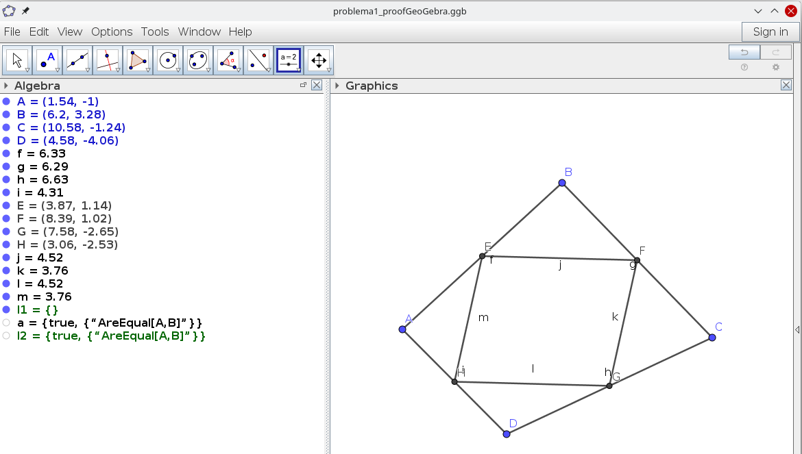
Figure 7: GeoGebra — Problem 1

B.2 JGEX

As can be seen in figure 8, with JGEX it is possible to have the visual checks, by moving the free points around, but also a formal proof, in this case using the geometry deductive database (GDD) method. It is possible to see the connection established between the construction and its rendering, and also between the proof and its visual rendering.

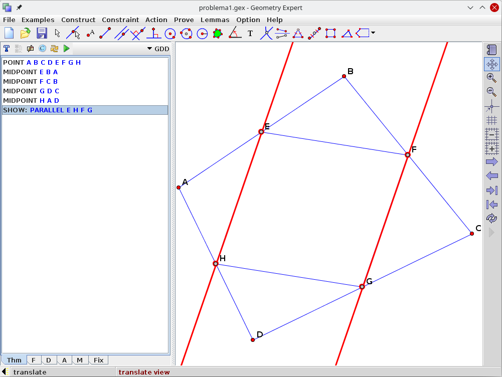
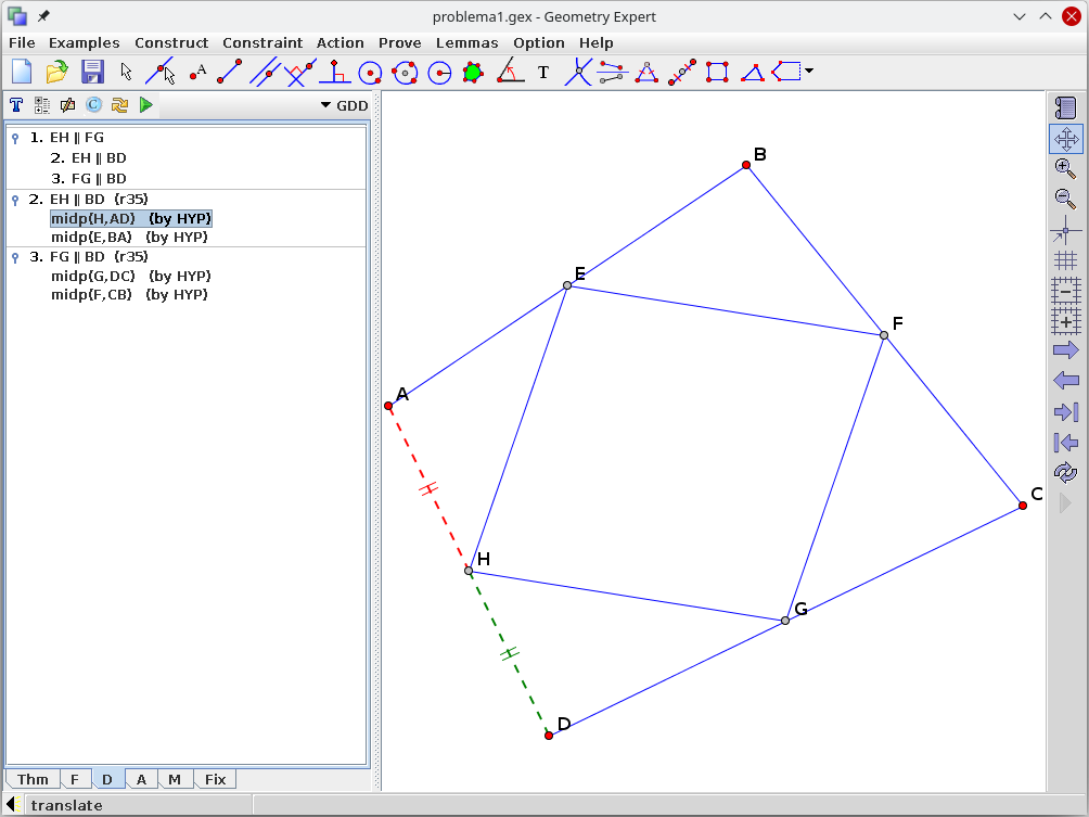
Figure 8: JGEX — Problem 1 — The conjecture (left), The Proof (right)

Unfortunately JGEX it is not being developed at this moment, but given that its authors took the decision of going open source, making available all the code in a GitHub repository it is possible that its development is resumed in the future.

B.3 GCLC

GCLC is more a GATP than a DGS. The geometric construction is written in the GCL language, it is rendered graphically, but there are no free points that can be moved around, enabling a visual verification of a given conjecture.

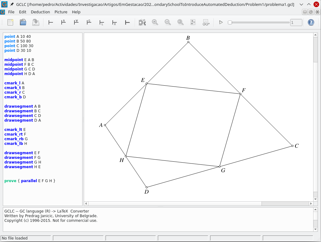
Figure 9: GCLC — Problem 1

Selecting one of its embedded GATP and processing the file, a readable proof script (in LaTeX) is produced. Unfortunately, readable here means, readable by experts, given that it is an algebraic proof (Wu’s method or Gröbner basis method) or it is a synthetic proof, but using a non-standard axiom system (area method). In table 3 an excerpt of the proof produced by GCLC area method prover is shown.

$$S_{EGH}=S_{FGH}\text{\parbox{96.00018pt}{by the statement{}}}$$ (1)

$$\left(S_{EGD}+\left(\frac{1}{2}\cdot\left(S_{EGA}+\left(-1\cdot S_{EGD}\right)\right)\right)\right)=S_{FGH}\text{\parbox{96.00018pt}{by Lemma 29 (point $H$ eliminated){}}}$$ (2)

$$\left(\left(\frac{1}{2}\cdot S_{EGD}\right)+\left(\frac{1}{2}\cdot S_{EGA}\right)\right)=S_{FGH}\text{\parbox{96.00018pt}{by algebraic simplifications{}}}$$ (3)

$$\left(\left(\frac{1}{2}\cdot S_{EGD}\right)+\left(\frac{1}{2}\cdot S_{EGA}\right)\right)=\left(S_{FGD}+\left(\frac{1}{2}\cdot\left(S_{FGA}+\left(-1\cdot S_{FGD}\right)\right)\right)\right)\text{\parbox{96.00018pt}{by Lemma 29 (point $H$ eliminated){}}}$$ (4)

$$\left(\left(\frac{1}{2}\cdot S_{DEG}\right)+\left(\frac{1}{2}\cdot S_{AEG}\right)\right)=\left(S_{DFG}+\left(\frac{1}{2}\cdot\left(S_{AFG}+\left(-1\cdot S_{DFG}\right)\right)\right)\right)\text{\parbox{96.00018pt}{by geometric simplifications{}}}$$ (5)

$$\left(S_{DEG}+S_{AEG}\right)=\left(S_{DFG}+S_{AFG}\right)\text{\parbox{96.00018pt}{by algebraic simplifications{}}}$$ (6)

$$\left(\left(S_{DEC}+\left(\frac{1}{2}\cdot\left(S_{DED}+\left(-1\cdot S_{DEC}\right)\right)\right)\right)+S_{AEG}\right)=\left(S_{DFG}+S_{AFG}\right)\text{\parbox{96.00018pt}{by Lemma 29 (point $G$ eliminated){}}}$$ (7)

$$\left(\left(S_{DEC}+\left(\frac{1}{2}\cdot\left(0+\left(-1\cdot S_{DEC}\right)\right)\right)\right)+S_{AEG}\right)=\left(S_{DFG}+S_{AFG}\right)\text{\parbox{96.00018pt}{by geometric simplifications{}}}$$ (8)

$$\left(\left(\frac{1}{2}\cdot S_{DEC}\right)+S_{AEG}\right)=\left(S_{DFG}+S_{AFG}\right)\text{\parbox{96.00018pt}{by algebraic simplifications{}}}$$ (9)

$$\left(\left(\frac{1}{2}\cdot S_{DEC}\right)+\left(S_{AEC}+\left(\frac{1}{2}\cdot\left(S_{AED}+\left(-1\cdot S_{AEC}\right)\right)\right)\right)\right)=\left(S_{DFG}+S_{AFG}\right)\text{\parbox{96.00018pt}{by Lemma 29 (point $G$ eliminated){}}}$$ (10)

Table 3: GCLC, Area Method Proof (excerpt) — Problem 1

The proof is 4 pages long, with 35 steps. The prover gives the following information at the end of the proof. “Q.E.D.” (or not proved, if that was the case) . There are no ndg (non-degenerated) conditions. Number of elimination proof steps: 12. Number of geometric proof steps: 21. Number of algebraic proof steps: 72. Total number of proof steps: 105. Time spent by the prover: 0.005 seconds.

B.4 Prover9

To be able to use Prover9 the full-angle method was converted to first-order form, TPTP/FOF syntax [26] and the geometric conjectures were also written in that language. A specific filter was used to convert that to Prover9 internal syntax.

⬇

% —Include Geometry Deductive Database Method axioms

include(’geometryDeductiveDatabaseMethod.ax’).

fof(tgtpproblema1,conjecture,( ! [ A,B,C,D] :

( midp(E,A,B) & midp(F,B,C) & midp(G,C,D) & midp(H,D,A) )

=>

( para(E,F,G,H) ) ) ).

The prover took 0.02s to prove it, producing a proof script (total of 1076 lines), with a final proof, short and readable, but not by secondary students nor by their teachers (without special training).

⬇

============================== PROOF =================================

% Proof 1 at 0.02 (+ 0.00) seconds.

% Length of proof is 7.

% Level of proof is 3.

% Maximum clause weight is 13.000.

% Given clauses 100.

64 (all A all B all C all D all M (midp(M,A,B) & midp(M,C,D) -> para(A,C,B,D)))

# label(ruleD63) # label(axiom) # label(non_clause). [assumption].

95 (all A all B all C all D (midp(E,A,B) & midp(F,B,C) & midp(G,C,D) &

midp(H,D,A))) -> para(E,F,G,H) # label(tgtpproblema1)

# label(conjecture) # label(non_clause) # label(goal). [goal].

166 -midp(A,B,C) | -midp(A,D,E) | para(B,D,C,E)

# label(ruleD63) # label(axiom). [clausify(64)].

208 midp(c1,A,B) # label(tgtpproblema1)

# label(conjecture). [deny(95)].

212 -para(c1,c2,c3,c4)

# label(tgtpproblema1) # label(conjecture). [deny(95)].

326 para(A,B,C,D). [resolve(208,a,166,b),unit_del(a,208)].

327 $F. [resolve(326,a,212,a)].

============================== end of proof ==========================

The use of FOF syntax allows the use of other generic ATP, for example, Vampire was also used, with similar results.

References

- [1]
- [2] Vincent Aleven, Octav Popescu & Kenneth R Koedinger (2001): Towards tutorial dialog to support self-explanation: Adding natural language understanding to a cognitive tutor. In: Proceedings of Artificial Intelligence in Education, pp. 246–255.
- [3] Francisco Botana, Markus Hohenwarter, Predrag Janičić, Zoltán Kovács, Ivan Petrović, Tomás Recio & Simon Weitzhofer (2015): Automated Theorem Proving in GeoGebra: Current Achievements. Journal of Automated Reasoning 55(1), pp. 39–59, 10.1007/s10817-015-9326-4.
- [4] Shang-Ching Chou & Xiao-Shan Gao (2001): Automated Reasoning in Geometry. In John Alan Robinson & Andrei Voronkov, editors: Handbook of Automated Reasoning, Elsevier Science Publishers B.V., pp. 707–749, 10.1016/B978-044450813-3/50013-8.
- [5] Shang-Ching Chou, Xiao-Shan Gao & Ji Zhang (1996): Automated Generation of Readable Proofs with Geometric Invariants, II. Theorem Proving With Full-Angles. Journal of Automated Reasoning 17, pp. 349–370, 10.1007/BF00283134.
- [6] Shang-Ching Chou, Xiao-Shan Gao & Jing-Zhong Zhang (2000): A Deductive Database Approach to Automated Geometry Theorem Proving and Discovering. Journal of Automated Reasoning 25(3), p. 219–246, 10.1023/A:1006171315513.
- [7] Pedro Cobo, Josep Fortuny, Eloi Puertas & Philippe Richard (2007): AgentGeom: a multiagent system for pedagogical support in geometric proof problems. International Journal of Computers for Mathematical Learning 12, pp. 57–79, 10.1007/s10758-007-9111-5.
- [8] Ludovic Font, Philippe R. Richard & Michel Gagnon (2018): Improving QED-Tutrix by Automating the Generation of Proofs. In Pedro Quaresma & Walther Neuper, editors: Proceedings 6th International Workshop on Theorem proving components for Educational software, Gothenburg, Sweden, 6 Aug 2017, Electronic Proceedings in Theoretical Computer Science 267, Open Publishing Association, pp. 38–58, 10.4204/EPTCS.267.3.
- [9] Herve Gallaire, Jack Minker & Jean-Marie Nicolas (1984): Logic and Databases: A Deductive Approach. ACM Computing Surveys 16(2), pp. 153–185, 10.1145/356924.356929.
- [10] Gila Hanna, David Reid & Michael de Villiers, editors (2019): Proof Technology in Mathematics Research and Teaching. Springer, 10.1007/978-3-030-28483-1.
- [11] Predrag Janičić (2010): Geometry Constructions Language. J. Autom. Reasoning 44(1-2), pp. 3–24. Available at http://dx.doi.org/10.1007/s10817-009-9135-8.
- [12] Predrag Janičić (2006): GCLC – A Tool for Constructive Euclidean Geometry and More Than That. In Andrés Iglesias & Nobuki Takayama, editors: Mathematical Software - ICMS 2006, Lecture Notes in Computer Science 4151, Springer, pp. 58–73, 10.1007/11832225_6.
- [13] Zoltán Kovács (2015): The Relation Tool in GeoGebra 5. In Francisco Botana & Pedro Quaresma, editors: Automated Deduction in Geometry, Lecture Notes in Computer Science 9201, Springer International Publishing, pp. 53–71, 10.1007/978-3-319-21362-0_4.
- [14] Zoltán Kovács & Jonathan H. Yu (2020): Towards Automated Discovery of Geometrical Theorems in GeoGebra. CoRR abs/2007.12447. Available at https://arxiv.org/abs/2007.12447.
- [15] Nicolas Leduc (2016): QED-Tutrix : système tutoriel intelligent pour l’accompagnement d’élèves en situation de résolution de problèmes de démonstration en géométrie plane. Ph.D. thesis, École polytechnique de Montréal.
- [16] Vanda Luengo (2005): Some didactical and epistemological considerations in the design of educational software: the Cabri-Euclide example. International Journal of Computers for Mathematical Learning 10(1), pp. 1–29, 10.1007/s10758-005-4580-x.
- [17] Constantino Martins, Paulo Couto, Marta Fernandes, Cristina Bastos, Cristina Lobo, Luiz Faria & Eurico Carrapatoso (2011): PCMAT–Mathematics Collaborative Learning Platform. In: Highlights in practical applications of agents and multiagent systems, Springer, pp. 93–100, 10.1007/978-3-642-19917-2_12.
- [18] Noboru Matsuda & Kurt VanLehn (2005): Advanced Geometry Tutor: An intelligent tutor that teaches proof-writing with construction. In Chee-Kit Looi, Gordon I. McCalla, Bert Bredeweg & Joost Breuker, editors: Artificial Intelligence in Education - Supporting Learning through Intelligent and Socially Informed Technology, Proceedings of the 12th International Conference on Artificial Intelligence in Education, AIED 2005, July 18-22, 2005, Amsterdam, The Netherlands, Frontiers in Artificial Intelligence and Applications 125, IOS Press, pp. 443–450. Available at http://www.booksonline.iospress.nl/Content/View.aspx?piid=1340.
- [19] Zoltán Kovács & Predrag Janičić Mladen Nikolić, Vesna Marinković (2019): Portfolio theorem proving and prover runtime prediction for geometry. Annals of Mathematics and Artificial Intelligence 85(2-4), pp. 119–146, 10.1007/s10472-018-9598-6.
- [20] Balacheff N. (2003): Ck, a knowledge model drawn from an understanding of students understanding. Didactical principles and model specifications. In: Soury-Lavergne S. (ed.) Baghera assessment project, designing an hybrid and emergent educational society. Technical Report 81, 3–22, Cahier Leibniz.
- [21] Art Quaife (1989): Automated development of Tarski’s geometry. Journal of Automated Reasoning 5, pp. 97–118, 10.1007/BF00245024.
- [22] Pedro Quaresma (2017): Towards an Intelligent and Dynamic Geometry Book. Mathematics in Computer Science 11(3), pp. 427–437, 10.1007/s11786-017-0302-8.
- [23] Philippe R Richard & Josep M Fortuny (2007): Amélioration des compétences argumentatives à l’aide d’un système tutoriel en classe de mathématique au secondaire. In: Annales de didactique et de sciences cognitives, 12, pp. 83–216.
- [24] Philippe R Richard, Josep M Fortuny, Markus Hohenwarter & Michel Gagnon (2007): geogebraTUTOR: une nouvelle approche pour la recherche sur l’apprentissage compétentiel et instrumenté de la géométrie à l’école secondaire. In: E-Learn: World Conference on E-Learning in Corporate, Government, Healthcare, and Higher Education, Association for the Advancement of Computing in Education (AACE), pp. 428–435.
- [25] Vanda Santos & Pedro Quaresma (forthcoming): Exploring Geometric Conjectures with the help of a Learning Environment - A Case Study with Pre-Service Teachers. The Electronic Journal of Mathematics and Technology 2(1).
- [26] G. Sutcliffe (2017): The TPTP Problem Library and Associated Infrastructure. From CNF to TH0, TPTP v6.4.0. Journal of Automated Reasoning 59(4), pp. 483–502, 10.1007/s10817-017-9407-7.
- [27] Ke Wang & Zhendong Su (2015): Automated Geometry Theorem Proving for Human-readable Proofs. In: Proceedings of the 24th International Conference on Artificial Intelligence, IJCAI’15, AAAI Press, pp. 1193–1199. Available at http://dl.acm.org/citation.cfm?id=2832249.2832414.
- [28] Zheng Ye, Shang-Ching Chou & Xiao-Shan Gao (2011): An Introduction to Java Geometry Expert. In Thomas Sturm & Christoph Zengler, editors: Automated Deduction in Geometry, Lecture Notes in Computer Science 6301, Springer Berlin Heidelberg, pp. 189–195, 10.1007/978-3-642-21046-4_10.