Nesterov Accelerated Shuffling Gradient Method for Convex Optimization

Abstract

In this paper, we propose Nesterov Accelerated Shuffling Gradient (NASG), a new algorithm for the convex finite-sum minimization problems. Our method integrates the traditional Nesterov’s acceleration momentum with different shuffling sampling schemes. We show that our algorithm has an improved rate of $\operatorname{\mathcal{O}}(1/T)$ using unified shuffling schemes, where $T$ is the number of epochs. This rate is better than that of any other shuffling gradient methods in convex regime. Our convergence analysis does not require an assumption on bounded domain or a bounded gradient condition. For randomized shuffling schemes, we improve the convergence bound further. When employing some initial condition, we show that our method converges faster near the small neighborhood of the solution. Numerical simulations demonstrate the efficiency of our algorithm.

1 Introduction

We consider the finite-sum optimization problem:

$$\min_{w\in\mathbb{R}^{d}}\left\{F(w):=\frac{1}{n}\sum_{i=1}^{n}f(w;i)\right\},$$ (1)

where the objective function $F:\mathbb{R}^{d}\to\mathbb{R}$ is smooth and convex, and each individual functions $f_{i}$ is smooth. This standard problem arises in most machine learning tasks, including logistic regression, multi-kernel learning, and some neural networks. The major challenge in solving (1) often comes from the high dimension space and a large number of components $n$. Therefore, deterministic methods relying on full gradients are usually inefficient to solve this problem (Sra et al., 2012; Bottou et al., 2018).

SGD and Shuffling SGD. Stochastic Gradient Descent (SGD) (Robbins & Monro, 1951) and its stochastic first-order variants have been widely used to solve (1) thanks to its scalability and efficiency in dealing with large-scale problems (Duchi et al., 2011; Kingma & Ba, 2014; Bottou et al., 2018; Nguyen et al., 2018).

At each iteration SGD samples an index $i$ uniformly from the set $\{1,\dots,n\}$, and uses the stochastic gradient $\nabla f_{i}$ to update the weight. While the uniformly independent sampling of $i$ plays an important role in our theoretical understanding of SGD, practical heuristics often use without-replacement sampling schemes (also known as shuffling sampling schemes). These methods depend on some random or deterministic permutations of the index set $\{1,2,\dots,n\}$ and apply incremental gradient updates using these permutation order. A collection of such $n$ individual updates is called an epoch, or a pass over all the data. The most popular method in this class is Random Reshuffling, which creates a new random permutation at the beginning of each epoch. Other important methods include Single Shuffling (which uses the same (random) permutation for each epoch) and Incremental Gradient (which uses a deterministic order of indices). In this paper, the term Shuffling SGD refers to SGD method using any data permutations, which includes the three special schemes described above.

Empirical studies show that shuffling sampling schemes usually provide a faster convergence than SGD (Bottou, 2009). However, due to the lack of statistical independence, analyzing these shuffling variants is often more challenging than the identically distributed version. Recent works have shown theoretical improvement for shuffling schemes over SGD in terms of the number of epochs needed to converge to an $\epsilon$-accurate solution (Gürbüzbalaban et al., 2019; Haochen & Sra, 2019; Safran & Shamir, 2020; Nagaraj et al., 2019; Rajput et al., 2020; Nguyen et al., 2021; Mishchenko et al., 2020; Ahn et al., 2020). In particular, in a general convex setting, shuffling sampling schemes improve the convergence rate of SGD from $\operatorname{\mathcal{O}}(1/\sqrt{T})$ to $\operatorname{\mathcal{O}}(1/T^{2/3})$ in terms of the number of effective data passes $T$ (Nguyen et al., 2021; Mishchenko et al., 2020). Thanks to their theoretical and empirical advantage, Random Reshuffling and its variants are becoming the methods of choice for practical implementation of machine learning optimization algorithms.

Nesterov’s Accelerated Gradient (NAG). On the other hand, one of the most beautiful idea in convex optimization is the Nesterov’s accelerated momentum technique, which was originally proposed in (Nesterov, 1983). The method, shown in Algorithm 1 for deterministic setting, achieves a much better convergence rate of $\operatorname{\mathcal{O}}(1/T^{2})$ than the convergence rate of Gradient Descent $\operatorname{\mathcal{O}}(1/T)$ in convex regimes, where $T$ is the total number of iterations. Note that the application of deterministic NAG requires a full gradient computation, i.e $n$ component gradients in each iteration, this $T$ is the same as the number of epochs.

Algorithm 1 Nesterov’s Accelerated Gradient (NAG)

1:  Initialization: Choose an initial point $x_{0},y_{0}\in\mathbb{R}^{d}$.

2:  for $t=1,2,\cdots,T$ do

3:     Let $x^{(t)}:=y^{(t-1)}-\alpha^{(t)}\nabla F(y^{(t-1)})$

4:     Compute $y^{(t)}:=x^{(t)}+\frac{t-1}{t+2}(x^{(t)}-x^{(t-1)})$

5:  end for

In the last two decades, researchers have made efforts to leverage this acceleration technique to the stochastic settings. It is well known that Stochastic Gradient Descent has the convergence rate of $\operatorname{\mathcal{O}}(1/\sqrt{K})$ where $K$ is the number of iterations. Vaswani et al. (2019) proposes to use a new assumption called the Strong Growth Condition for which they can prove an accelerated rate of SGD with Nesterov’s momentum. This condition implies that the stochastic gradients (and, hence, its variance) converge to zero at the optimum (Schmidt & Roux, 2013; Vaswani et al., 2019). However, without a strong assumption on the gradient oracle (i.e. without assuming that the variance goes to zero), no work has been able to prove a better convergence rate for SGD with Nesterov’s momentum over the ordinary results of SGD (Hu et al., 2009; Lan, 2012). This background along with the theoretical advances of Shuffling SGD motivates the central question of our paper:

Can we use Nesterov’s momentum technique for Shuffling SGD to improve the convergence rate using only standard assumptions (e.g. without assuming vanishing variance)?

We answer this question positively in this paper; our results are summarized below.

Summary of our contributions.

• We propose Nesterov Accelerated Shuffling Gradient (NASG) method, a new algorithm to approximate the solution of the convex minimization problem (1). Our method integrates the well-known Nesterov’s acceleration technique with shuffling sampling strategies. In stead of the traditional practice that add momentum term in each iteration, we adopt a new approach that integrates the momentum for each training epoch.

• We establish the convergence analysis for our algorithm in the convex setting using standard assumptions, i.e. generalized bounded variance or convex component functions. Our method achieves an improved rate of $\operatorname{\mathcal{O}}(1/T)$ in terms of the number of epochs for the unified shuffling schemes. We also investigate the randomized schemes (including Random Reshuffling and Single Shuffling) and improve a factor of $n$ in the convergence bound. Moreover, our convergence results work for the last iterate returned by the algorithm, which is more practical than previous works for the average iterate.

• We test our algorithms via numerical simulations on various machine learning tasks and compare them with other stochastic first order methods. Our tests have shown good overall performance of the new algorithms.

Related work. Let us briefly review the most related works to our methods studied in this paper.

Shuffling SGD schemes. In the big data machine learning setting, Random Reshuffling and Single Shuffling are more favorable than plain SGD thanks to their better practical performance and simple implementation (Bottou, 2009, 2012; Recht & Ré, 2011). While the convergence properties of SGD are well-understood in literature, the theoretical analysis for the randomized shuffling schemes remained challenging for a long period of time. A natural reason behind this problem is the lack of conditionally unbiased gradients: $\mathbb{E}\left[\nabla f(y_{i}^{(t)};\pi_{i}^{(t)})\right]\neq\nabla F(y_{i}^{(t)}),$ where $t$ is the current epoch. Recently, researchers have made progress in the analysis of convergence rates of randomized shuffling techniques (Gürbüzbalaban et al., 2019; Haochen & Sra, 2019; Safran & Shamir, 2020; Nagaraj et al., 2019; Ahn et al., 2020). with the majority of these works devoted to the strongly convex case (with a bounded gradient or bounded domain assumption). The best known convergence rate in this case is $\operatorname{\mathcal{O}}(1/(nT)^{2}+1/(nT^{3}))$ where $T$ is the number of epochs. This result matches the lower bound rate in (Safran & Shamir, 2020) up to some constant factor.

Table 1: Number of individual gradient evaluations needed by SGD-type algorithms to reach an $\epsilon$-accurate solution $x$ that satisfies $F(x)-F(x_{*})\leq\epsilon$. In this table, $L$ is the Lipschitz constant in Assumption 3.1, $\sigma_{*}^{2}$ is the variance at the minimizer $x_{*}$ defined in (4). Finally, $\Delta:=\|\tilde{x}_{0}-x_{*}\|^{2}$ is the squared distance from the initial point $\tilde{x}_{0}$ to the minimizer $x_{*}$.

Algorithms	Complexity	References
Standard SGD(1)	$\operatorname{\mathcal{O}}\left(\frac{\Delta_{0}^{2}+G^{2}}{\epsilon^{2}}\right)$ (1)	(Nemirovski et al., 2009; Shamir & Zhang, 2013)
SGD - Unified Schemes(2)	$\operatorname{\mathcal{O}}\left(\frac{nL\Delta}{\epsilon}+\frac{n\sqrt{L}\sigma_{*}\Delta}{\epsilon^{3/2}}\right)$	(Mishchenko et al., 2020; Nguyen et al., 2021)
SGD - Randomized Schemes(3)	$\operatorname{\mathcal{O}}\left(\frac{nL\Delta}{\epsilon}+\frac{\sqrt{nL}\sigma_{*}\Delta}{\epsilon^{3/2}}\right)$	(Mishchenko et al., 2020)
NASG - Unified Schemes	$\operatorname{\mathcal{O}}\left(\frac{nL\Delta}{\epsilon}+\frac{n\sigma_{*}^{2}}{L\epsilon}\right)$	(This work, Theorem 4.1 and Corollary B.2)
NASG - Randomized Schemes(3)	$\operatorname{\mathcal{O}}\left(\frac{nL\Delta}{\epsilon}+\frac{\sigma_{*}^{2}}{L\epsilon}\right)$	(This work, Theorem 4.5 and Corollary D.3)

⁽¹⁾ Standard results for SGD in literature often use a different set of assumptions from the one in this paper (e.g. bounded domain that $\|x-x_{*}\|^{2}\leq\Delta_{0}$ for each iterate $x$ and/or bounded gradient that $\mathbb{E}[\|\nabla f(x;i)\|]\leq G^{2}$). We report the corresponding complexity for a rough comparison. ⁽²⁾ (Mishchenko et al., 2020) shows a bound for Incremental Gradient while (Nguyen et al., 2021) has a unified setting. We translate these results for Unified Schemes from these references to our convex setting. ⁽³⁾ While using the same set of assumptions, the convergence criteria for randomized schemes is in expectation form: $\mathbb{E}[F(x)-F(x_{*})]\leq\epsilon$.

In the convex regime, most dominant results are originally derived for the deterministic Incremental Gradient scheme (Nedic & Bertsekas, 2001a, b). More recent works investigate convergence theory for various shuffling schemes (Shamir, 2016; Mishchenko et al., 2020; Nguyen et al., 2021), where Nguyen et al. (2021) provides a unified approach to different shuffling schemes and proves the convergence rate of $\operatorname{\mathcal{O}}(1/T^{2/3})$. When a randomized scheme is applied (Random Reshuffling or Single Shuffling), the bound in expectation improves to $\operatorname{\mathcal{O}}(1/T+1/(n^{1/3}T^{2/3}))$. For a comparison, our Algorithm 2 developed in this paper achieves a deterministic convergence rate of $\operatorname{\mathcal{O}}(1/T)$ for the same setting under standard assumptions. The computational complexity for these methods are in Table 1.

In the meantime, a popular line of research involves variance reduction technique, which have shown encouraging performance for machine learning (e.g., SAG (Le Roux et al., 2012), SAGA (Defazio et al., 2014), SVRG (Johnson & Zhang, 2013) and SARAH (Nguyen et al., 2017)). These methods need to either compute or store a full gradient or a large batch of gradient. This plays an important role in reducing the variance and therefore, is the key factor for these methods. However, the update of SGD, Shuffling SGD and our Algorithm 2 does not require full gradient evaluation at any stage. Thus, our new Algorithm 2 belongs to the class of Shuffling SGD which deviates from variance reduction methods.

Momentum Techniques. The most popular and successful momentum techniques include the classical Heavy-ball method (Polyak, 1964) and Nesterov’s acceleration gradient (NAG) (Nesterov, 1983, 2004). Although these two methods are different, they both receive great attention in the optimization community (Hu et al., 2009; Lan, 2012; Sutskever et al., 2013; Yuan et al., 2016; Dozat, 2016). Nesterov’s acceleration method is well-known for its improved convergence rate of $\operatorname{\mathcal{O}}(1/T^{2})$ (versus the $\operatorname{\mathcal{O}}(1/T)$ of Gradient Descent) for general smooth convex functions in the deterministic setting, where $T$ is the number of iterations.

On the other hand, Devolder et al. (2014) and Lessard et al. (2016) suggest that Nesterov’s acceleration is not robust to the errors in gradient and its performance may be worse than gradient descent due to error accumulation. A more recent work (Liu & Belkin, 2018) argues that stochastic NAG does not provide acceleration over ordinary SGD in general, and may diverge for step sizes that guarantee convergence of SGD. These observations further motivate our algorithmic design for the Shuffling SGD with Nesterov’s momentum in Section 2.

2 Nesterov Accelerated Shuffling Gradient Method

In this section, we describe our new shuffling gradient algorithm with Nesterov’s momentum in Algorithm 2.

Before we start, it should be noted that the classical approach in stochastic NAG literature is applying the momentum term for each iteration (Hu et al., 2009; Lan, 2012; Zhong & Kwok, 2014; Vaswani et al., 2019). However, empirical evidence have shown that Nesterov’s acceleration may not be superior when inexact gradients are used, and the reason might be error accumulation (Devolder et al., 2014; Liu & Belkin, 2018). In addition, while SGD has access to an unbiased estimator for the full gradient, shuffling gradient schemes generally do not have this property. In consequence, updating the momentum at each inner iteration is less preferable since it could make the estimator deviate from the true gradient and further accumulate errors.

Based on these observations, we adopt a different approach to update the Nesterov’s momentum after each epoch which consists of $n$ gradients. This practice allows our method to approximate the full gradient more accurately while still maintains the effectiveness of the momentum technique. It is also consistent with the application of Heavy-ball method and proximal operator for shuffling schemes in recent literature (Tran et al., 2021; Mishchenko et al., 2021). Our algorithm is presented below.

Algorithm 2 Nesterov Accelerated Shuffling Gradient (NASG) Method

1:  Initialization: Choose an initial point $\tilde{x}_{0},\tilde{y}_{0}\in\mathbb{R}^{d}$.

2:  for $t=1,2,\cdots,T$ do

3:     Set $y_{0}^{(t)}:=\tilde{y}_{t-1}$;

4:     Generate any permutation $\pi^{(t)}$ of $[n]$ (either deterministic or random);

5:     for $i=1,\cdots,n$ do

6:        Update $y_{i}^{(t)}:=y_{i-1}^{(t)}-\eta_{i}^{(t)}\nabla f(y_{i-1}^{(t)};\pi^{(t)}(i))$;

7:     end for

8:     Set $\tilde{x}_{t}:=y_{n}^{(t)}$;

9:     Update $\tilde{y}_{t}:=\tilde{x}_{t}+\gamma_{t}(\tilde{x}_{t}-\tilde{x}_{t-1})$;

10:  end for

Algorithm Description. In each epoch $t$, our method first performs $n$ consecutive individual gradient updates in variable $y_{i}^{(t)}$ following a permutation $\pi^{(t)}$ of the index set $\{1,\dots,n\}$. At the end of each epoch, it applied the Nesterov’s momentum update using an auxiliary variable $\tilde{x}_{t}$. The choice of learning rate $\eta_{i}^{(t)}$ is further specified in our theoretical analysis.

The per-iteration complexity of Algorithm 2 is the same as standard shuffling gradient schemes (Shamir, 2016). In addition, our algorithm only requires a storage cost of $\operatorname{\mathcal{O}}(d)$, which is similar to that of standard SGD. Note that the implementation of our method requires neither full gradient computation nor a large batch of gradient computation at any point. Our convergence guarantee in Theorem 4.1 and Theorem 4.3 for unified shuffling scheme holds for any permutation of $\{1,2,\cdots,n\}$, including deterministic and random ones. Therefore, our method works for any shuffling strategy, including Incremental Gradient, Single Shuffling, and Random Reshuffling.

Comparison with Nesterov’s Accelerated Gradient. Let us recall that deterministic NAG has an update of full gradient computation from $y^{(t-1)}$ to $x^{(t)}$. We can write this update in a different way, where $y^{(t-1)}=y_{0}^{(t)}$ and each component gradient at $y_{0}^{(t)}$ is gradually computed and subtracted from the starting point:

1:  for $i=1,\cdots,n$ do

2:     Update $y_{i}^{(t)}:=y_{i-1}^{(t)}-\eta_{i}^{(t)}\nabla f({\color[rgb]{0,0,1}y_{0}^{(t)}};\pi^{(t)}(i))$;

3:  end for

With an appropriate choice of learning rates, at the end of an epoch, the output $y_{n}^{(t)}$ in this representation is identical to the output $x^{(t)}$ of deterministic NAG algorithm. This illustrates the comparison between traditional NAG and our method. While NAG only update the weights after a full gradient computation, our method gradually updates and makes movement after each component evaluations.

In order to motivate our Algorithm 2, we conduct a small binary classification experiment and demonstrate the behaviour of NAG and the stochastic momentum methods. The details of the settings are delayed to Section 5.1. Figure 1 shows that applying Nesterov’s momentum term for each iteration may accumulate errors and lead to a poor result. While the deterministic NAG converges and slowly decreases the loss, our stochastic version works faster and achieves an overall better performance, when the number of data $n$ is large.

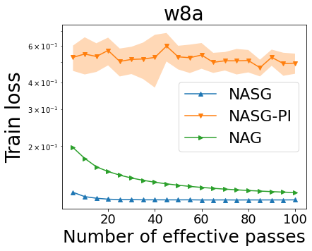
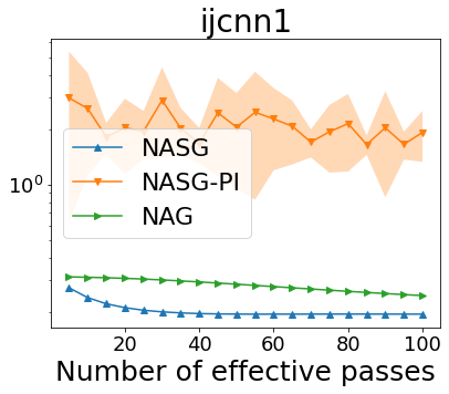
Figure 1: Comparisons of the training loss for w8a and ijcnn1 datasets. NAG denotes the deterministic Nesterov’s Accelerated Gradient. NASG is our method, while NASG-PI is the stochastic shuffling version that applies Nesterov’s momentum each inner iteration. We apply random reshuffling schemes for the stochastic algorithms.

3 Technical Settings

3.1 Theoretical Assumptions

We analyze the convergence of Algorithm 2 under standard assumptions, which are presented below. Our first assumption is that all component functions are $L$-smooth.

Assumption 3.1.

We assume that $f(\cdot;i)$ is $L$-smooth for every $i\in[n]$, i.e., there exists a constant $L>0$ such that, $\forall x,y\in\mathbb{R}^{d}$,

$$\|\nabla f(x;i)-\nabla f(y;i)\|\leq L\|x-y\|,\ i\in[n].$$ (2)

Assumption 3.1 implies that $F$ is also $L$-smooth. This assumption is widely used in literature for gradient-type methods in both stochastic and deterministic settings. Then, by a well-known property of $L$-smooth functions in (Nesterov, 2004), we have, $\forall x,y\in\mathbb{R}^{d}$,

$$F(x) \leq F(y)+\langle\nabla F(y),(x-y)\rangle+\frac{L}{2}\|x-y\|^{2}.$$ (3)

Our main results for Algorithm 2 is in convex setting which requires the following assumption.

Assumption 3.2.

$f(\cdot;i)$ is convex for every $i\in[n]$, i.e., $\forall x,y\in\mathbb{R}^{d}$,

$$f(x;i)-f(y;i)\geq\langle\nabla f(y;i),(x-y)\rangle,\ i\in[n].$$

When $F$ is convex, we also assume that the existence of a minimizer for $F$. Note that $F$ could have more than one minimizer. Therefore, in this paper, we let $x_{*}$ be any minimizer of $F$ and consider the corresponding variance of $F$ at $x_{*}$:

$$\sigma_{*}^{2}:=\frac{1}{n}\sum_{i=1}^{n}\|\nabla{f}(x_{*};i)\|^{2}\in[0,+\infty).$$ (4)

Alternatively, when each individual function $f(\cdot;i)$ is not necessary convex and $F$ is convex, we consider the following assumption:

Assumption 3.3.

(Generalized bounded variance) There exist two non-negative and finite constants $\Theta$ and $\sigma$ such that for any $x\in\mathbb{R}^{d}$ we have

$$\frac{1}{n}\sum_{i=1}^{n}\|\nabla f(x;i)-\nabla F(x)\|^{2}\leq\Theta\|\nabla F(x)\|^{2}+\sigma^{2}.$$ (5)

Assumption 3.3 reduces to the standard bounded variance condition if $\Theta=0$. Therefore, it is more general than the bounded variance assumption, which is often used in stochastic optimization (Bottou et al., 2018).

3.2 Basic Derivations

In this section, we provide some key derivations for Algorithm 2. From the update of our algorithm and the choice $\gamma_{t}=\frac{t-1}{t+2}$, we have for $t\geq 1$

$$\tilde{y}_{t}:=\tilde{x}_{t}+\frac{t-1}{t+2}(\tilde{x}_{t}-\tilde{x}_{t-1}).$$ (6)

Similar to the original Nesterov’s momentum technique, we use two following auxiliary variables in our analysis:

$$\theta^{(t)}=\frac{2}{t+2}\in(0,1),\text{ and }v^{(t)}=\frac{t+1}{2}\tilde{x}_{t}-\frac{t-1}{2}\tilde{x}_{t-1},$$

for $t\geq 1$. We also use the convention that $\theta^{(0)}=1$ and $v^{(0)}=\tilde{x}_{0}$. This is equivalent to

$$\tilde{x}_{t} =\frac{2}{t+1}v^{(t)}+\frac{t-1}{t+1}\tilde{x}_{t-1}$$

$$=\theta^{(t-1)}v^{(t)}+(1-\theta^{(t-1)})\tilde{x}_{t-1}.$$ (7)

This property shows that $\tilde{x}_{t}$ is a convex combination of $v^{(t)}$ and $\tilde{x}_{t-1}$ for every iteration $t\geq 1$. Using equation (6), we further have

$$\tilde{y}_{t} =\tilde{x}_{t}+\frac{t-1}{t+2}(\tilde{x}_{t}-\tilde{x}_{t-1})$$

$$=\frac{t+1}{t+2}\tilde{x}_{t}-\frac{t-1}{t+2}\tilde{x}_{t-1}+\frac{t}{t+2}\tilde{x}_{t}$$

$$=\frac{2}{t+2}\left(\frac{t+1}{2}\tilde{x}_{t}-\frac{t-1}{2}\tilde{x}_{t-1}\right)+\left(1-\frac{2}{t+2}\right)\tilde{x}_{t}$$

$$=\theta^{(t)}v^{(t)}+(1-\theta^{(t)})\tilde{x}_{t}.$$ (8)

Again, $\tilde{y}_{t}$ is a convex combination of $v^{(t)}$ and $\tilde{x}_{t}$, however with a slightly different parameter $\theta^{(t)}$ instead of $\theta^{(t-1)}$.

These key derivations play an important role in the theoretical analysis of Algorithm 2. They help explain why Nesterov’s momentum can achieve a better convergence rate when the objective function $F$ is convex. Indeed, using convexity of $F$ we have the following property:

$$F(y)+\langle\nabla F(y),(1-\theta)x+\theta x_{*}-y\rangle$$

$$\leq\ F((1-\theta)x+\theta x_{*})\leq(1-\theta)F(x)+\theta F(x_{*})$$

for any $x\in\mathbb{R}^{d}$, $y\in\mathbb{R}^{d}$, and $\theta\in[0,1]$. The application of this inquality is the central idea behind our theoretical results, which are presented in the next section.

4 Theoretical Analysis

4.1 Convergence Rate for Unified Shuffling Scheme

In this section, we investigate the theoretical performance of Algorithm 2 using unified shuffling strategy, i.e. using an arbitrary permutation $\pi^{(t)}$ in any of the epoch $t=1,2,\dots,T$. These permutations can be random or deterministic, however our results hold deterministically regardless of the choice of permutation. We first establish the convergence for Algorithm 2 under the condition that all the component functions are convex.

Theorem 4.1 (Convex component functions).

Suppose that Assumption 3.1 and 3.2 hold for (1). Let $\{x_{i}^{(t)}\}$ be generated by Algorithm 2 with parameter $\gamma_{t}=\frac{t-1}{t+2}$, the learning rate $\eta_{i}^{(t)}:=\frac{\eta_{t}}{n}>0$ for $\eta_{t}=\frac{k\alpha^{t}}{LT}\leq\frac{1}{L}$ where $k=\frac{1}{e\alpha\sqrt[3]{12}}>0$ and $\alpha=1+\frac{1}{T}>0$. Then for $T\geq 2$ we have

$$F(\tilde{x}_{T})-F(x_{*}) \leq\frac{4\sigma_{*}^{2}}{9LT}+\frac{2Le\sqrt[3]{12}}{T}\|\tilde{x}_{0}-x_{*}\|^{2}.$$ (9)

Remark 4.2.

The convergence rate of Algorithm 2 is exactly expressed as

$$\operatorname{\mathcal{O}}\left(\frac{\sigma_{*}^{2}/L+L\|\tilde{x}_{0}-x_{*}\|^{2}}{T}\right),$$

which is better than the state-of-the-art rate in the literature (Mishchenko et al., 2020; Nguyen et al., 2021) in term of $T$ for convex problems with general shuffling-type strategies. Translating this convergence rate to computational complexity, we get the results in Table 1. We provide the proof of Theorem 4.1 and its complexity in the Appendix.

When the component functions are not necessarily convex, we establish the convergence for Algorithm 2 under the convexity of $F$ and the generalized bounded variance assumption.

Theorem 4.3 (Generalized Bounded Variance).

Suppose that Assumption 3.1 and 3.3 hold for (1). In addition, we assume that $F$ is convex. Let $\{x_{i}^{(t)}\}$ be generated by Algorithm 2 with parameter $\gamma_{t}=\frac{t-1}{t+2}$, the learning rate $\eta_{i}^{(t)}:=\frac{\eta_{t}}{n}>0$ for $\eta_{t}=\frac{k\alpha^{t}}{LT}\leq\frac{1}{L}$ where $k=\frac{1}{e\alpha\sqrt[3]{2(6\Theta+7)}}>0$ and $\alpha=1+\frac{1}{T}>0$. Then for $T\geq 2$, $F(\tilde{x}_{T})-F(x_{*})$ is upper bounded by

$$\frac{8\sigma^{2}}{3(6\Theta+7)LT}+\frac{2Le\sqrt[3]{2(6\Theta+7)}}{T}\|\tilde{x}_{0}-x_{*}\|^{2}.$$

The convergence rate of Theorem 4.3 is expressed as

$$\operatorname{\mathcal{O}}\left(\frac{\sigma^{2}/(\Theta L)+L\Theta^{1/3}\|\tilde{x}_{0}-x_{*}\|^{2}}{T}\right),$$

which is similar to the convergence rate $\operatorname{\mathcal{O}}\left(1/T\right)$ of Theorem 4.1. We defer the proof of Theorem 4.5 to Appendix.

Remark 4.4 (Convergence guarantee).

Our convergence bounds in Theorem 4.1 and 4.3 hold in a deterministic sense. This convergence criteria for Algorithm 2 is significantly stronger than the standard criteria in expectation for other SGD-type algorithm in literature recently (Ghadimi & Lan, 2013; Shamir & Zhang, 2013). This improvement is made thanks to the unique structure of the Nesterov’s acceleration applied to Shuffling schemes in our Algorithm 2. In addition, our results hold for the last iterate $x_{T}$, which matches the practical heuristics more than previous results that hold for an average $\tilde{x}$ of training weights $x_{1},\dots,x_{T}$ (Polyak & Juditsky, 1992; Ghadimi & Lan, 2013).

4.2 Convergence Rate for Randomized Schemes

We continue to present the theoretical result of Algorithm 2 specifically for Randomized Schemes, namely Random Reshuffling and Single Shuffling schemes where random permutation(s) are generated for the update of Algorithm 2. Our next Theorem 4.5 uses the assumption that all the component functions are convex.

Theorem 4.5 (Randomized Schemes).

Suppose that Assumption 3.1 and 3.2 hold for (1). Let $\{x_{i}^{(t)}\}$ be generated by Algorithm 2 under a randomized scheme with parameter $\gamma_{t}=\frac{t-1}{t+2}$, the learning rate $\eta_{i}^{(t)}:=\frac{\eta_{t}}{n}>0$ for $\eta_{t}=\frac{k\alpha^{t}}{LT}\leq\frac{1}{L}$ where $k=\frac{1}{e\alpha\sqrt[3]{12}}>0$ and $\alpha=1+\frac{1}{T}>0$. Then for $T\geq 2$, we have

$$\mathbb{E}[F(\tilde{x}_{T})-F(x_{*})] \leq\frac{8\sigma_{*}^{2}}{27nLT}+\frac{2Le\sqrt[3]{12}}{T}\|\tilde{x}_{0}-x_{*}\|^{2}.$$ (10)

Remark 4.6 (Randomized Schemes).

The convergence rate of Theorem 4.5 is expressed as

$$\operatorname{\mathcal{O}}\left(\frac{\sigma_{*}^{2}/L}{nT}+\frac{L\|\tilde{x}_{0}-x_{*}\|^{2}}{T}\right),$$

which is better than the state-of-the-art rate for randomized schemes in the literature (Mishchenko et al., 2020; Nguyen et al., 2021) for convex problems.

Comparing to the unified case, our result allows a reduction in the first term of the bound by a factor of $n$. This fact is essentially helpful in machine learning applications where the number of data $n$ is large. Furthermore, in practice randomized schemes offer a lot of improvements when the variance at the optimizer $\sigma_{*}^{2}$ can be large. Similar to the previous theorems, our result in Theorem 4.5 holds for the last iterate $x_{T}$, which matches the practical heuristics. We defer the proof of this theorem to the Appendix.

4.3 Improved Convergence Rate with Initial Condition

In this section, we consider an initial condition where the iterate of our algorithm is in a small neighborhood of the optimal point. Let us note that the minimizer of $F$ may not be unique, hence we only requires this assumption for some minimizer $x_{*}$.

Remark 4.7.

Let us assume that $\|\tilde{x}_{0}-x_{*}\|\leq\frac{E}{\sqrt{n}}$ where $\tilde{x}_{0}$ be the initial point and $E>0$ be a constant. For the same conditions as in Theorem 4.1, i.e. component convexity, we have

$$F(\tilde{x}_{T})-F(x_{*})\leq\operatorname{\mathcal{O}}\left(\frac{\sigma_{*}^{2}/L+LE^{2}}{n^{3/4}T}\right),$$ (11)

which has an improvement of $n^{3/4}$ over the plain setting of Theorem 4.1. This fact suggests that the algorithm may converge faster when it reaches a small neighborhood of the solution set. The proof of this Remark requires some modifications from Theorem 4.1, and is presented in Appendix.

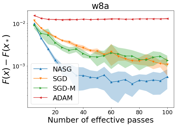
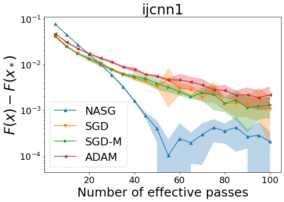
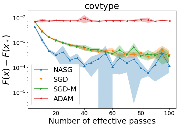
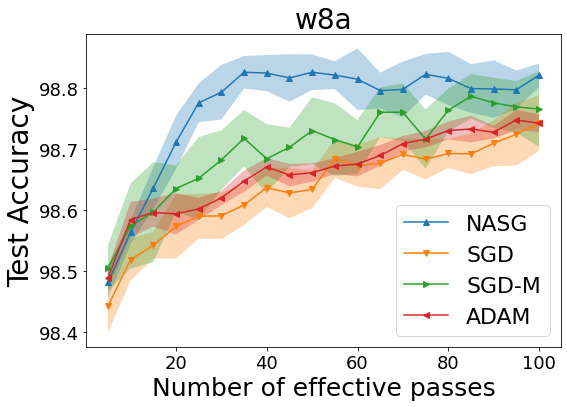
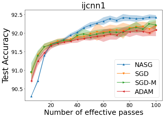
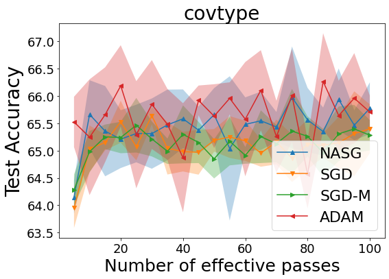
Figure 2: (Convex binary setting). Comparisons of loss residual $F(x)-F(x_{*})$ (top) and test accuracy (bottom) produced by first-order methods for w8a, ijcnn1 and covtype datasets, respectively. The number of effective passes is the number of epochs (i.e. number of data passes) in the progress.

Remark 4.8.

Let us assume that $\|\tilde{x}_{0}-x_{*}\|\leq\frac{E}{\sqrt{n}}$ where $\tilde{x}_{0}$ be the initial point and $E>0$ be a constant. For the same conditions as in Theorem 4.5, i.e. component convexity with a randomized scheme, we have

$$\mathbb{E}\left[F(\tilde{x}_{T})-F(x_{*})\right]\leq\operatorname{\mathcal{O}}\left(\frac{\sigma_{*}^{2}/L+LE^{2}}{nT}\right),$$ (12)

which shows a further improvement of $n$ over the standard setting thanks to the application of randomized schemes and initial assumption.

5 Numerical Experiments

To support our theoretical analysis, we present three sets of numerical experiments, comparing our algorithm with the state-of-the-art SGD-type and shuffling gradient methods.

5.1 Binary Classification

In this section, we describe the setting of Figure 1 and other experiments. Let us consider the following convex binary classification problem:

$$\min_{w\in\mathbb{R}^{d}}\Big{\{}F(w)\!:=\!\frac{1}{n}\sum_{i=1}^{n}\log(1\!+\!\exp(-y_{i}x_{i}^{\top}w))\!\Big{\}},$$

where $\{(x_{i},y_{i})\}_{i=1}^{n}$ is a set of training samples with $x_{i}\in\mathbb{R}^{d}$ and $y_{i}\in\{-1,1\}$. We have conducted the experiments on three classification datasets w8a ($49,749$ samples), ijcnn1 ($91,701$ samples) and covtype ($406709$ samples) from LIBSVM (Chang & Lin, 2011). The stochastic experiments are repeated with random seeds 10 times and we report the average results with confidence intervals.

In Figure 1, we compare our algorithm with NAG and the stochastic shuffling version that update Nesterov’s momentum per iteration. Note that NAG is a deterministic algorithm, hence it does not have confidence intervals. In order to make fair comparisons, we report the results of three methods in Figure 1 after every effective data passes, (i.e. comparing them with the same computational cost). In addition, since NAG converges slowly when $n$ is large, in our futher experiments, we choose to compare our algorithm with other stochastic first-order methods.

In Figure 2, we compare our method with Stochastic Gradient Descent (SGD) and two stochastic algorithms: SGD with Momentum (SGD-M) (Polyak, 1964) and Adam (Kingma & Ba, 2014). For the latter two algorithms, we use the hyper-parameter settings recommended and widely used in practice (i.e. momentum: 0.9 for SGD-M, and two hyper-parameters $\beta_{1}:=0.9$, $\beta_{2}:=0.999$ for Adam).

To have a fair comparison, we apply the randomized reshuffling scheme to all methods. Note that shuffling strategies are favorable in practice and have been implemented in TensorFlow, PyTorch, and Keras (Abadi et al., 2015; Paszke et al., 2019; Chollet et al., 2015). We tune each algorithm using constant learning rate and report the best final results.

For w8a and covtype datasets, our algorithm shows better performance than the other methods in the training process. For ijcnn1, NASG is somewhat worse than the other methods at the beginning, however, it surpasses all other methods after a few epochs and maintains a better decrease toward the end of training stage. In terms of test accuracy, our method shows comparable performance for covtype dataset, and achieves good generalization for w8a and ijcnn1 datasets.

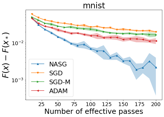
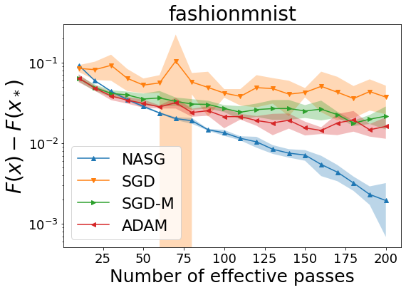
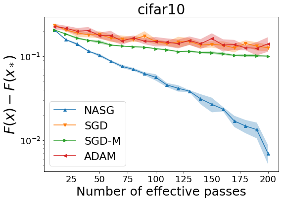
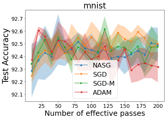
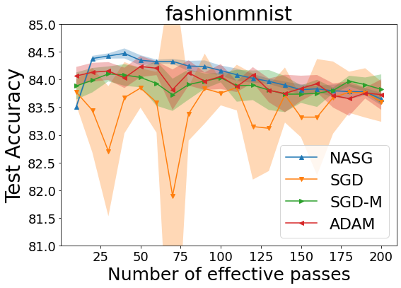
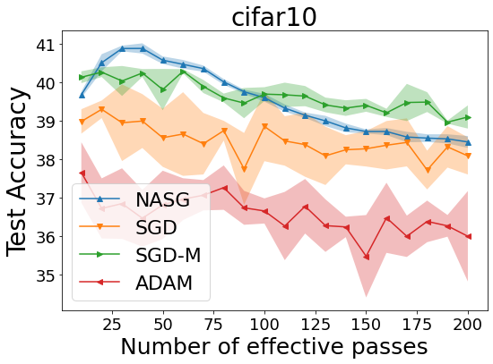
Figure 3: (Convex image setting). Comparisons of loss residual $F(x)-F(x_{*})$ (top) and test accuracy (bottom) produced by first-order methods for MNIST, Fashion-MNIST and CIFAR-10, respectively. The number of effective passes is the number of epochs (i.e. number of data passes) throughout the progress.

In the next subsection, we perform another set of experiments in convex setting. Our Appendix describes all the experimental details and implementation.

5.2 Convex Image Classification

For the second experiment, we test our algorithm using linear neural networks on three well-known image classification datasets: MNIST dataset (LeCun et al., 1998) and Fashion-MNIST dataset (Xiao et al., 2017) both with $60,000$ samples, and finally CIFAR-10 dataset (Krizhevsky & Hinton, 2009) with $50,000$ images. We experiment with the following minimization problem:

$$\min_{w\in\mathbb{R}^{d}}\Big{\{}F(w):=-\frac{1}{n}\sum_{i=1}^{n}y_{i}^{\top}\log(\text{softmax}(h(w;i)))\Big{\}},$$

where $h(w;i)=Wx_{i}+b$ is a simple neural network with parameter $w=\{W,b\},$ $W\in\mathbb{R}^{c\times d}$ and $b\in\mathbb{R}^{c}$. The input data $\{x_{i}\}_{i=1}^{n}$ are in $\mathbb{R}^{d}$ and the output labels $\{y_{i}\}_{i=1}^{n}$ are one-hot vectors in $\mathbb{R}^{c}$, where $c$ is the number of classes. The softmax function is defined as

$$\text{softmax}(z)=\left(\frac{e^{z_{1}}}{\sum_{k=1}^{c}e^{z_{k}}};\dots;\frac{e^{z_{c}}}{\sum_{k=1}^{c}e^{z_{k}}}\right)^{\top}.$$

Similar to the previous experiment, we compare our algorithm with other stochastic first-order methods with randomized reshuffling scheme. The minibatch size is 256. All the algorithms are implemented in Python using PyTorch package (Paszke et al., 2019). They are tested using 10 different random seeds and we report the average results with confidence intervals. We tune each algorithm using constant learning rate and report the best final results in Figure 3.

Our algorithm achieves a better decrease than other methods on MNIST and CIFAR-10 datasets very early in the training process. On Fashion-MNIST dataset, NASG starts slower than other methods at the beginning. In the next stage, it suggests a better performance with a little oscillations in the end.

In terms of generalization, our method shows comparable performance to all other stochastic algorithms. Note that our main focus is the training task, that is, solving the optimization problem (1) and there may be over-fitting that leads to test accuracy decrease in the later part of the training progress.

5.3 Non-convex Image Classification

We further test our algorithm with a simple non-convex model to demonstrate the efficiency and flexibility of our method beyond the convex setting. For this experiment, we use a similar problem as in the previous section (i.e. training neural networks on three image classification datasets: MNIST, Fashion-MNIST dataset and CIFAR-10 dataset). The minimization problem is:

$$\min_{w\in\mathbb{R}^{d}}\Big{\{}F(w):=-\frac{1}{n}\sum_{i=1}^{n}y_{i}^{\top}\log(\text{softmax}(h(w;i)))\Big{\}},$$

where $h(w;i)=W_{2}(W_{1}x_{i}+b_{1})+b_{2}$ is a neural network with one hidden layer containing $m$ neurons and no activation. The input data $\{x_{i}\}_{i=1}^{n}$ are in $\mathbb{R}^{d}$ and the output labels $\{y_{i}\}_{i=1}^{n}$ are one-hot vectors in $\mathbb{R}^{c}$, where $c$ is the number of classes. The parameter is $w=\{W_{1},b_{1},W_{2},b_{2}\}$ with $W_{1}\in\mathbb{R}^{m\times d},b_{1}\in\mathbb{R}^{m}$ and $W_{2}\in\mathbb{R}^{c\times m},b_{2}\in\mathbb{R}^{c}$.

For MNIST and Fashion-MNIST datasets, we run a small network with $m=300$ hidden neurons. For CIFAR-10 dataset, we experiment with $m=900$ neurons in the hidden layer. Similar to the previous experiments, we compare our algorithm with other stochastic first-order methods (SGD, SGD-M and ADAM) and we apply randomized reshuffling scheme to all these algorithms. We implement all the methods in Python using PyTorch package (Paszke et al., 2019), then tune each algorithm using constant learning rate. Figure 4 report the train loss and the squared norm of gradient returned by our experiments. We delay other experimental setting details to the Appendix.

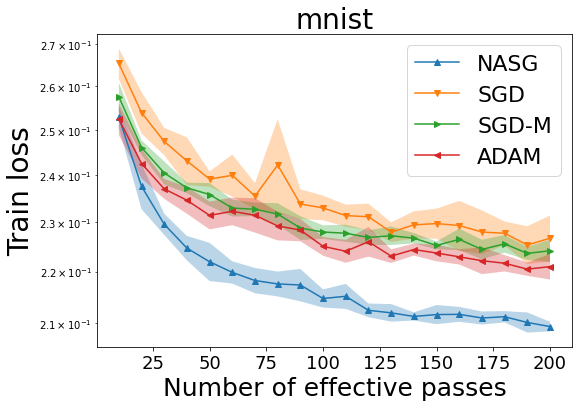
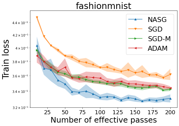
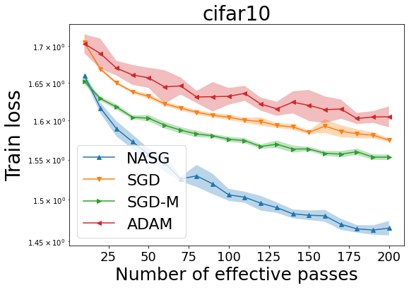
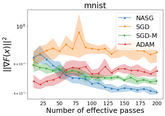
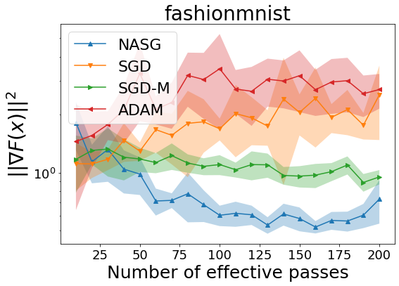
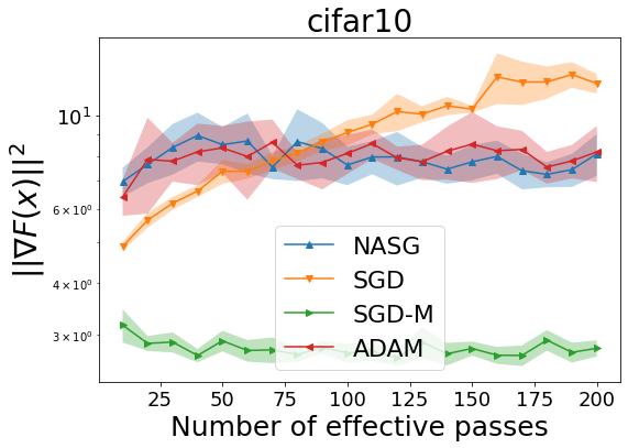
Figure 4: (Non-convex image setting). Comparisons of train loss $F(x)$ (top) and the squared norm of gradient $\|\nabla F(x)\|^{2}$ produced by first-order methods for MNIST, Fashion-MNIST and CIFAR-10, respectively. The number of effective passes is the number of epochs (i.e number of data passes) throughout the progress.

In this simple non-convex setting, our algorithm also achieves a better decrease than other methods on MNIST and CIFAR-10 datasets. On Fashion-MNIST dataset, NASG starts slower than other methods at the beginning and surpasses other method later in the training process. In terms of gradient norm, our method shows competitive performance for MNIST and Fashion-MNIST datasets, while performs comparably good in CIFAR-10 dataset. We further note that all our experiments are tuned to the best value of the training loss for every algorithm.

6 Conclusions and Future Work

We propose Nesterov Accelerated Shuffling Gradient (NASG), a new gradient method that combines the update of SGD using shuffling sampling schemes with Nesterov’s momentum. Our method achieves a convergence rate of $\operatorname{\mathcal{O}}(1/T)$ for smooth convex functions, where $T$ is the number of effective data passes. This rate is better than the state-of-the-art result of SGD using shuffling schemes, in terms of $T$.

Although we have made progresses in understanding theoretical properties of shuffling methods in general (and NASG in particular), an interesting research question remains: whether our method can achieve a better theoretical rate in terms of the number of data points $n$. Our work answers this question partially by different approaches, including the application of randomized sampling schemes and the investigation of an initial condition. In addition, investigating our algorithm in non-convex settings is also a promising direction.

Appendix A Technical Lemmas

A.1 Basic Derivations for Algorithm 2

Let us collect all the basic necessary expressions for Algorithm 2. From the update $y_{i}^{(t)}:=y_{i-1}^{(t)}-\eta_{i}^{(t)}\nabla f(y_{i-1}^{(t)};\pi^{(t)}(i))$, we have the following for $i=1,\dots,n,t\geq 1$:

$$y_{i}^{(t)}=y_{i-1}^{(t)}-\eta_{i}^{(t)}\nabla f(y_{i-1}^{(t)};\pi^{(t)}(i))=y_{0}^{(t)}-\sum_{j=1}^{i}\eta_{j}^{(t)}\nabla f(y_{j-1}^{(t)};\pi^{(t)}(j)).$$ (13)

Note that $y_{0}^{(t)}=\tilde{y}_{t-1}$ and $\tilde{x}_{t}=y_{n}^{(t)}$ and $\eta_{i}^{(t)}=\frac{\eta_{t}}{n}$ for $i=1,\dots,n,t\geq 1$, we have

$$\tilde{x}_{t}=\tilde{y}_{t-1}-\frac{\eta_{t}}{n}\sum_{j=1}^{n}\nabla f(y_{j-1}^{(t)};\pi^{(t)}(j)).$$ (14)

From (7) and (8) we have the following for $t\geq 1$:

$$\tilde{x}_{t+1}=\tilde{y}_{t}+\theta^{(t)}(v^{(t+1)}-v^{(t)}).$$ (15)

On the other hand, we consider the term $v^{(t+1)}=\frac{t+2}{2}\tilde{x}_{t+1}-\frac{t}{2}\tilde{x}_{t}$ for $t\geq 0$:

$$\frac{t+2}{2}\tilde{x}_{t+1}-\frac{t}{2}\tilde{x}_{t} \overset{\eqref{eq_004}}{=}\frac{t+2}{2}\left(\tilde{y}_{t}-\frac{\eta_{t+1}}{n}\sum_{j=1}^{n}\nabla f(y_{j-1}^{(t+1)};\pi^{(t+1)}(j))\right)-\frac{t}{2}\tilde{x}_{t}$$

$$\overset{\eqref{eq_005}}{=}\frac{t+2}{2}\left(\tilde{x}_{t}+\frac{t-1}{t+2}(\tilde{x}_{t}-\tilde{x}_{t-1})-\frac{\eta_{t+1}}{n}\sum_{j=1}^{n}\nabla f(y_{j-1}^{(t+1)};\pi^{(t+1)}(j))\right)-\frac{t}{2}\tilde{x}_{t}$$

$$=\left(\frac{t+1}{2}\tilde{x}_{t}-\frac{t-1}{2}\tilde{x}_{t-1}\right)-\left(\frac{t+2}{2}\right)\frac{\eta_{t+1}}{n}\sum_{j=1}^{n}\nabla f(y_{j-1}^{(t+1)};\pi^{(t+1)}(j)).$$

Therefore by definitions of $v^{(t)}$ and $\theta^{(t)}$ we have

$$v^{(t+1)} =v^{(t)}-\frac{\eta_{t+1}}{\theta^{(t)}}\cdot\frac{1}{n}\sum_{j=1}^{n}\nabla f(y_{j-1}^{(t+1)};\pi^{(t+1)}(j)),\ t\geq 0.$$ (16)

Using convexity of $F$, for any $x\in\mathbb{R}^{d}$, $y\in\mathbb{R}^{d}$, and $\theta\in[0,1]$, we have

$$(1-\theta)F(x)+\theta F(x_{*})\geq F((1-\theta)x+\theta x_{*})\geq F(y)+\langle\nabla F(y),(1-\theta)x+\theta x_{*}-y\rangle,$$

where $x_{*}=\arg\min_{x}F(x)$ is an optimal solution of $F$. Hence,

$$F(y)\leq(1-\theta)F(x)+\theta F(x_{*})+\langle\nabla F(y),y-(1-\theta)x-\theta x_{*}\rangle.$$ (17)

In addition, we define the following term:

$$K_{t} =\frac{1}{n}\sum_{i=1}^{n}\left\|y_{i}^{(t)}-y_{0}^{(t)}\right\|^{2}\text{ and }I_{t}=\frac{1}{n}\sum_{i=1}^{n}\left\|y_{n}^{(t)}-y_{i}^{(t)}\right\|^{2}.$$

For each epoch $t=1,\cdots,T$, we denote $\mathcal{F}_{t}$ by $\sigma(y_{0}^{(1)},\cdots,y_{0}^{(t)})$, the $\sigma$-algebra generated by the iterates of Algorithm 2 up to the beginning of the epoch $t$.We also denote $\mathbb{E}_{t}[\cdot]$ by $\mathbb{E}[\cdot\mid\mathcal{F}_{t}]$, the conditional expectation on the $\sigma$-algebra $\mathcal{F}_{t}$.

A.2 Key Lemmas and Proofs of Key Lemmas

Lemma A.1.

Suppose that Assumption 3.1 holds for (1), and $F$ is convex. Let $\{\tilde{x}_{t}\}$ be generated by Algorithm 2 with the learning rate $\eta_{i}^{(t)}:=\frac{\eta_{t}}{n}>0$ for a given positive sequence $\{\eta_{t}\}$ with $\eta_{t}\leq\frac{1}{L}$. Let $\epsilon_{t}$ be a positive sequence, $t\geq 1$. Then we have the following for $t\geq 1$:

$$T(T+2)[F(\tilde{x}_{T})-F(x_{*})] \leq\sum_{t=1}^{T}\frac{L^{2}\eta_{t}(t+1)^{2}}{2\epsilon_{t}}K_{t}-\sum_{t=1}^{T}[F(\tilde{x}_{t})-F(x_{*})]$$

$$\qquad+\sum_{t=1}^{T}\frac{2}{\eta_{t}}\|v^{(t-1)}-x_{*}\|^{2}-\sum_{t=1}^{T}\frac{2}{\eta_{t}}(1-\epsilon_{t})\|v^{(t)}-x_{*}\|^{2}.$$ (18)

Proof of Lemma A.1: Key estimate for Algorithm 2

We start with the update (14) of Algorithm 2, for $t\geq 1$:

$$F(\tilde{x}_{t}) \overset{\eqref{eq_004}}{=}F\left(\tilde{y}_{t-1}-\frac{\eta_{t}}{n}\sum_{j=1}^{n}\nabla f(y_{j-1}^{(t)};\pi^{(t)}(j))\right)$$

$$\overset{\eqref{eq:Lsmooth}}{\leq}F(\tilde{y}_{t-1})-\eta_{t}\left\langle\nabla F(\tilde{y}_{t-1}),\frac{1}{n}\sum_{j=1}^{n}\nabla f(y_{j-1}^{(t)};\pi^{(t)}(j))\right\rangle+\frac{L\eta_{t}^{2}}{2}\left\|\frac{1}{n}\sum_{j=1}^{n}\nabla f(y_{j-1}^{(t)};\pi^{(t)}(j))\right\|^{2}$$

$$\overset{\eqref{eq_008},\eqref{eq_006}}{\leq}(1-\theta^{(t-1)})F(\tilde{x}_{t-1})+\theta^{(t-1)}F(x_{*})+\langle\nabla F(\tilde{y}_{t-1}),\theta^{(t-1)}v^{(t-1)}-\theta^{(t-1)}x_{*}\rangle$$

$$\qquad-\eta_{t}\left\langle\nabla F(\tilde{y}_{t-1}),\frac{1}{n}\sum_{j=1}^{n}\nabla f(y_{j-1}^{(t)};\pi^{(t)}(j))\right\rangle+\frac{\eta_{t}}{2}\left\|\frac{1}{n}\sum_{j=1}^{n}\nabla f(y_{j-1}^{(t)};\pi^{(t)}(j))\right\|^{2},$$

where the last line follows since $\eta_{t}\leq\frac{1}{L}$. We further have

$$F(\tilde{x}_{t}) \leq(1-\theta^{(t-1)})F(\tilde{x}_{t-1})+\theta^{(t-1)}F(x_{*})$$

$$\qquad+\left\langle\nabla F(\tilde{y}_{t-1})-\frac{1}{n}\sum_{j=1}^{n}\nabla f(y_{j-1}^{(t)};\pi^{(t)}(j)),\theta^{(t-1)}(v^{(t-1)}-x_{*})\right\rangle$$

$$\qquad+\left\langle\frac{1}{n}\sum_{j=1}^{n}\nabla f(y_{j-1}^{(t)};\pi^{(t)}(j)),\theta^{(t-1)}(v^{(t-1)}-x_{*})\right\rangle$$

$$\qquad-\eta_{t}\left\langle\nabla F(\tilde{y}_{t-1})-\frac{1}{n}\sum_{j=1}^{n}\nabla f(y_{j-1}^{(t)};\pi^{(t)}(j)),\frac{1}{n}\sum_{j=1}^{n}\nabla f(y_{j-1}^{(t)};\pi^{(t)}(j))\right\rangle$$

$$\qquad-\eta_{t}\left\|\frac{1}{n}\sum_{j=1}^{n}\nabla f(y_{j-1}^{(t)};\pi^{(t)}(j))\right\|^{2}+\frac{\eta_{t}}{2}\left\|\frac{1}{n}\sum_{j=1}^{n}\nabla f(y_{j-1}^{(t)};\pi^{(t)}(j))\right\|^{2}$$

$$\overset{\eqref{eq_007}}{=}(1-\theta^{(t-1)})F(\tilde{x}_{t-1})+\theta^{(t-1)}F(x_{*})$$

$$\qquad+\left\langle\nabla F(\tilde{y}_{t-1})-\frac{1}{n}\sum_{j=1}^{n}\nabla f(y_{j-1}^{(t)};\pi^{(t)}(j)),\theta^{(t-1)}(v^{(t)}-x_{*})\right\rangle$$

$$\qquad+\left\langle\frac{1}{n}\sum_{j=1}^{n}\nabla f(y_{j-1}^{(t)};\pi^{(t)}(j)),\theta^{(t-1)}(v^{(t-1)}-x_{*})\right\rangle$$

$$\qquad-\frac{\eta_{t}}{2}\left\|\frac{1}{n}\sum_{j=1}^{n}\nabla f(y_{j-1}^{(t)};\pi^{(t)}(j))\right\|^{2}$$

$$=(1-\theta^{(t-1)})F(\tilde{x}_{t-1})+\theta^{(t-1)}F(x_{*})$$

$$\qquad+\left\langle\nabla F(\tilde{y}_{t-1})-\frac{1}{n}\sum_{j=1}^{n}\nabla f(y_{j-1}^{(t)};\pi^{(t)}(j)),\theta^{(t-1)}(v^{(t)}-x_{*})\right\rangle$$

$$\qquad+\frac{(\theta^{(t-1)})^{2}}{2\eta_{t}}\Big{[}\frac{2\eta_{t}}{\theta^{(t-1)}}\left\langle\frac{1}{n}\sum_{j=1}^{n}\nabla f(y_{j-1}^{(t)};\pi^{(t)}(j)),(v^{(t-1)}-x_{*})\right\rangle$$

$$\qquad-\left(\frac{\eta_{t}}{\theta^{(t-1)}}\right)^{2}\left\|\frac{1}{n}\sum_{j=1}^{n}\nabla f(y_{j-1}^{(t)};\pi^{(t)}(j))\right\|^{2}+\|v^{(t-1)}-x_{*}\|^{2}-\|v^{(t-1)}-x_{*}\|^{2}\Big{]}$$

$$\overset{\eqref{eq_007}}{=}(1-\theta^{(t-1)})F(\tilde{x}_{t-1})+\theta^{(t-1)}F(x_{*})$$

$$\qquad+\left\langle\nabla F(\tilde{y}_{t-1})-\frac{1}{n}\sum_{j=1}^{n}\nabla f(y_{j-1}^{(t)};\pi^{(t)}(j)),\theta^{(t-1)}(v^{(t)}-x_{*})\right\rangle$$

$$\qquad+\frac{(\theta^{(t-1)})^{2}}{2\eta_{t}}\Big{[}\|v^{(t-1)}-x_{*}\|^{2}-\|v^{(t)}-x_{*}\|^{2}\Big{]},$$ (19)

where we apply equation (16).

By the definition $K_{t}=\frac{1}{n}\sum_{i=1}^{n}\left\|y_{i}^{(t)}-y_{0}^{(t)}\right\|^{2}$, we get that

$$\left\|\nabla F(\tilde{y}_{t-1})-\frac{1}{n}\sum_{j=1}^{n}\nabla f(y_{j-1}^{(t)};\pi^{(t)}(j))\right\|^{2} =\left\|\frac{1}{n}\sum_{j=1}^{n}\left(\nabla f(\tilde{y}_{t-1};\pi^{(t)}(j))-\nabla f(y_{j-1}^{(t)};\pi^{(t)}(j))\right)\right\|^{2}$$

$$\leq\frac{1}{n}\sum_{j=1}^{n}\left\|\nabla f(\tilde{y}_{t-1};\pi^{(t)}(j))-\nabla f(y_{j-1}^{(t)};\pi^{(t)}(j))\right\|^{2}$$

$$\overset{\eqref{eq:Lsmooth}}{\leq}L^{2}\frac{1}{n}\sum_{j=1}^{n}\left\|y_{0}^{(t)}-y_{j-1}^{(t)}\right\|^{2}$$

$$\leq\frac{L^{2}}{n}\sum_{i=1}^{n}\left\|y_{i}^{(t)}-y_{0}^{(t)}\right\|^{2}=L^{2}K_{t}.$$ (20)

From (19) and using the inequality $\langle a,b\rangle\leq\frac{\|a\|^{2}}{2\epsilon_{t}}+\frac{\epsilon_{t}\|b\|^{2}}{2}$ for any $\epsilon_{t}>0$, we have

$$F(\tilde{x}_{t})-F(x_{*}) \leq(1-\theta^{(t-1)})[F(\tilde{x}_{t-1})-F(x_{*})]$$

$$\qquad+\left\langle\nabla F(\tilde{y}_{t-1})-\frac{1}{n}\sum_{j=1}^{n}\nabla f(y_{j-1}^{(t)};\pi^{(t)}(j)),\theta^{(t-1)}(v^{(t)}-x_{*})\right\rangle$$

$$\qquad+\frac{(\theta^{(t-1)})^{2}}{2\eta_{t}}\Big{[}\|v^{(t-1)}-x_{*}\|^{2}-\|v^{(t)}-x_{*}\|^{2}\Big{]}$$

$$\leq(1-\theta^{(t-1)})[F(\tilde{x}_{t-1})-F(x_{*})]$$

$$\qquad+\frac{\eta_{t}}{2\epsilon_{t}}\left\|\nabla F(\tilde{y}_{t-1})-\frac{1}{n}\sum_{j=1}^{n}\nabla f(y_{j-1}^{(t)};\pi^{(t)}(j))\right\|^{2}+\frac{\epsilon_{t}(\theta^{(t-1)})^{2}}{2\eta_{t}}\left\|v^{(t)}-x_{*}\right\|^{2}$$

$$\qquad+\frac{(\theta^{(t-1)})^{2}}{2\eta_{t}}\Big{[}\|v^{(t-1)}-x_{*}\|^{2}-\|v^{(t)}-x_{*}\|^{2}\Big{]}$$

$$\overset{\eqref{eq_015}}{\leq}(1-\theta^{(t-1)})[F(\tilde{x}_{t-1})-F(x_{*})]+\frac{L^{2}\eta_{t}}{2\epsilon_{t}}K_{t}$$

$$\qquad+\frac{(\theta^{(t-1)})^{2}}{2\eta_{t}}\|v^{(t-1)}-x_{*}\|^{2}-\frac{(\theta^{(t-1)})^{2}}{2\eta_{t}}(1-\epsilon_{t})\|v^{(t)}-x_{*}\|^{2}.$$

Now substituting $\theta^{(t)}=\frac{2}{t+2}$, $\theta^{(t-1)}=\frac{2}{t+1}$ we get

$$F(\tilde{x}_{t})-F(x_{*}) \leq\frac{t-1}{t+1}[F(\tilde{x}_{t-1})-F(x_{*})]+\frac{L^{2}\eta_{t}}{2\epsilon_{t}}K_{t}$$

$$\qquad+\frac{2}{\eta_{t}(t+1)^{2}}\|v^{(t-1)}-x_{*}\|^{2}-\frac{2}{\eta_{t}(t+1)^{2}}(1-\epsilon_{t})\|v^{(t)}-x_{*}\|^{2}.$$ (21)

Multiplying two sides by $(t+1)^{2}$ we have

$$(t+1)^{2}[F(\tilde{x}_{t})-F(x_{*})] \leq(t-1)(t+1)[F(\tilde{x}_{t-1})-F(x_{*})]+\frac{L^{2}\eta_{t}(t+1)^{2}}{2\epsilon_{t}}K_{t}$$

$$\qquad+\frac{2}{\eta_{t}}\|v^{(t-1)}-x_{*}\|^{2}-\frac{2}{\eta_{t}}(1-\epsilon_{t})\|v^{(t)}-x_{*}\|^{2}.$$

Summing the previous expression from $t=1$ to $t=T$ we get that

$$\sum_{t=1}^{T}(t+1)^{2}[F(\tilde{x}_{t})-F(x_{*})] \leq\sum_{t=1}^{T}(t^{2}-1)[F(\tilde{x}_{t-1})-F(x_{*})]+\sum_{t=1}^{T}\frac{L^{2}\eta_{t}(t+1)^{2}}{2\epsilon_{t}}K_{t}$$

$$\qquad+\sum_{t=1}^{T}\frac{2}{\eta_{t}}\|v^{(t-1)}-x_{*}\|^{2}-\sum_{t=1}^{T}\frac{2}{\eta_{t}}(1-\epsilon_{t})\|v^{(t)}-x_{*}\|^{2},$$

which is equivalent to

$$\sum_{t=1}^{T}[(t+1)^{2}-1][F(\tilde{x}_{t})-F(x_{*})] \leq\sum_{t=1}^{T}(t^{2}-1)[F(\tilde{x}_{t-1})-F(x_{*})]+\sum_{t=1}^{T}\frac{L^{2}\eta_{t}(t+1)^{2}}{2\epsilon_{t}}K_{t}$$

$$\qquad+\sum_{t=1}^{T}\frac{2}{\eta_{t}}\|v^{(t-1)}-x_{*}\|^{2}-\sum_{t=1}^{T}\frac{2}{\eta_{t}}(1-\epsilon_{t})\|v^{(t)}-x_{*}\|^{2}-\sum_{t=1}^{T}[F(\tilde{x}_{t})-F(x_{*})].$$

Hence we get the desired estimate of Lemma A.1:

$$T(T+2)[F(\tilde{x}_{T})-F(x_{*})] \leq\sum_{t=1}^{T}\frac{L^{2}\eta_{t}(t+1)^{2}}{2\epsilon_{t}}K_{t}-\sum_{t=1}^{T}[F(\tilde{x}_{t})-F(x_{*})]$$

$$\qquad+\sum_{t=1}^{T}\frac{2}{\eta_{t}}\|v^{(t-1)}-x_{*}\|^{2}-\sum_{t=1}^{T}\frac{2}{\eta_{t}}(1-\epsilon_{t})\|v^{(t)}-x_{*}\|^{2}.$$ (22)

$\square$

Lemma A.2.

Suppose that Assumption 3.1 holds for (1). Let $\{\tilde{x}_{t}\}$ be generated by Algorithm 2 with the learning rate $\eta_{i}^{(t)}:=\frac{\eta_{t}}{n}>0$ for a given positive sequence $\{\eta_{t}\}$ with $\eta_{t}\leq\frac{1}{2L}$. Then we have the following for $t\geq 1$:

$$K_{t}\leq\frac{8\eta_{t}^{2}}{n^{3}}\sum_{i=1}^{n-1}\left\|\sum_{j=i+1}^{n}\nabla f(\tilde{x}_{t};\pi^{(t)}(j))\right\|^{2}+4\eta_{t}^{2}\left\|\nabla F(\tilde{x}_{t})\right\|^{2}.$$ (23)

Proof of Lemma A.2: Bound the term $K_{t}$

Let us recall the definition of $K_{t}$ and $I_{t}$:

$$K_{t} =\frac{1}{n}\sum_{i=1}^{n}\left\|y_{i}^{(t)}-y_{0}^{(t)}\right\|^{2},\text{ and }I_{t}=\frac{1}{n}\sum_{i=1}^{n}\left\|y_{n}^{(t)}-y_{i}^{(t)}\right\|^{2}.$$

We consider the individual squared term of $I_{t}$:

$$\left\|y_{n}^{(t)}-y_{i}^{(t)}\right\|^{2} =\frac{\eta_{t}^{2}}{n^{2}}\left\|\sum_{j=i+1}^{n}\nabla f(y_{j-1}^{(t)};\pi^{(t)}(j))\right\|^{2}$$

$$=\frac{\eta_{t}^{2}}{n^{2}}\left\|\sum_{j=i+1}^{n}\nabla f(y_{j-1}^{(t)};\pi^{(t)}(j))-\sum_{j=i+1}^{n}\nabla f(y_{n}^{(t)};\pi^{(t)}(j))+\sum_{j=i+1}^{n}\nabla f(y_{n}^{(t)};\pi^{(t)}(j))\right\|^{2}$$

$$\leq\frac{2\eta_{t}^{2}}{n^{2}}\left\|\sum_{j=i+1}^{n}\nabla f(y_{j-1}^{(t)};\pi^{(t)}(j))-\sum_{j=i+1}^{n}\nabla f(y_{n}^{(t)};\pi^{(t)}(j))\right\|^{2}+\frac{2\eta_{t}^{2}}{n^{2}}\left\|\sum_{j=i+1}^{n}\nabla f(y_{n}^{(t)};\pi^{(t)}(j))\right\|^{2}$$

$$\leq\frac{2\eta_{t}^{2}}{n^{2}}(n-i)\sum_{j=i+1}^{n}\left\|\nabla f(y_{j-1}^{(t)};\pi^{(t)}(j))-\nabla f(y_{n}^{(t)};\pi^{(t)}(j))\right\|^{2}+\frac{2\eta_{t}^{2}}{n^{2}}\left\|\sum_{j=i+1}^{n}\nabla f(y_{n}^{(t)};\pi^{(t)}(j))\right\|^{2},$$

where in the last two lines we use the inequality $(u+v)^{2}\leq 2u^{2}+2v^{2}$ and Cauchy-Schwartz inequality. From Assumption 3.1 we have

$$\left\|y_{n}^{(t)}-y_{i}^{(t)}\right\|^{2} \leq\frac{2\eta_{t}^{2}}{n^{2}}(n-i)\sum_{j=i+1}^{n}\left\|\nabla f(y_{j-1}^{(t)};\pi^{(t)}(j))-\nabla f(y_{n}^{(t)};\pi^{(t)}(j))\right\|^{2}+\frac{2\eta_{t}^{2}}{n^{2}}\left\|\sum_{j=i+1}^{n}\nabla f(y_{n}^{(t)};\pi^{(t)}(j))\right\|^{2}$$

$$\overset{\eqref{eq:Lsmooth}}{\leq}\frac{2L^{2}\eta_{t}^{2}}{n^{2}}(n-i)\sum_{j=i+1}^{n}\left\|y_{j-1}^{(t)}-y_{n}^{(t)}\right\|^{2}+\frac{2\eta_{t}^{2}}{n^{2}}\left\|\sum_{j=i+1}^{n}\nabla f(y_{n}^{(t)};\pi^{(t)}(j))\right\|^{2}$$

$$\leq\frac{2L^{2}\eta_{t}^{2}}{n^{2}}(n-i)nI_{t}+\frac{2\eta_{t}^{2}}{n^{2}}\left\|\sum_{j=i+1}^{n}\nabla f(y_{n}^{(t)};\pi^{(t)}(j))\right\|^{2},$$

where last inequality follows from definition of $I_{t}$. Summing up the previous expression from $i=1$ to $i=n-1$ we get

$$nI_{t}=\sum_{i=1}^{n-1}\left\|y_{n}^{(t)}-y_{i}^{(t)}\right\|^{2} \leq\frac{2L^{2}\eta_{t}^{2}}{n^{2}}\sum_{i=1}^{n-1}(n-i)nI_{t}+\frac{2\eta_{t}^{2}}{n^{2}}\sum_{i=1}^{n-1}\left\|\sum_{j=i+1}^{n}\nabla f(y_{n}^{(t)};\pi^{(t)}(j))\right\|^{2}$$

$$\leq\frac{2L^{2}\eta_{t}^{2}}{n^{2}}\frac{n^{2}}{2}nI_{t}+\frac{2\eta_{t}^{2}}{n^{2}}\sum_{i=1}^{n-1}\left\|\sum_{j=i+1}^{n}\nabla f(y_{n}^{(t)};\pi^{(t)}(j))\right\|^{2}$$

$$\leq L^{2}\eta_{t}^{2}nI_{t}+\frac{2\eta_{t}^{2}}{n^{2}}\sum_{i=1}^{n-1}\left\|\sum_{j=i+1}^{n}\nabla f(y_{n}^{(t)};\pi^{(t)}(j))\right\|^{2},$$

where we use the fact that $\sum_{i=1}^{n-1}(n-i)\leq\frac{n^{2}}{2}$. Since $\eta_{t}\leq\frac{1}{2L}$, we have $\eta_{t}^{2}L^{2}\leq\frac{1}{4}$. Hence

$$\frac{3}{4}nI_{t} \leq\frac{2\eta_{t}^{2}}{n^{2}}\sum_{i=1}^{n-1}\left\|\sum_{j=i+1}^{n}\nabla f(y_{n}^{(t)};\pi^{(t)}(j))\right\|^{2},$$

and equivalently

$$I_{t} \leq\frac{8\eta_{t}^{2}}{3n^{3}}\sum_{i=1}^{n-1}\left\|\sum_{j=i+1}^{n}\nabla f(y_{n}^{(t)};\pi^{(t)}(j))\right\|^{2}.$$ (24)

For $i=0$ we have

$$\left\|y_{n}^{(t)}-y_{0}^{(t)}\right\|^{2} \leq\frac{2L^{2}\eta_{t}^{2}}{n^{2}}n^{2}I_{t}+\frac{2\eta_{t}^{2}}{n^{2}}\left\|\sum_{j=1}^{n}\nabla f(y_{n}^{(t)};\pi^{(t)}(j))\right\|^{2}$$

$$\overset{\eqref{eq_021}}{\leq}2L^{2}\eta_{t}^{2}I_{t}+\frac{2\eta_{t}^{2}}{n^{2}}\left\|\sum_{j=1}^{n}\nabla f(y_{n}^{(t)};\pi^{(t)}(j))\right\|^{2}$$

$$\leq\frac{1}{2}I_{t}+2\eta_{t}^{2}\left\|\nabla F(y_{n}^{(t)})\right\|^{2}.$$ (25)

Now we are ready to investigate $K_{t}$. By inequality $(u+v)^{2}\leq 2u^{2}+2v^{2}$ we get

$$K_{t}=\frac{1}{n}\sum_{i=1}^{n}\left\|y_{i}^{(t)}-y_{0}^{(t)}\right\|^{2} \leq\frac{1}{n}\sum_{i=1}^{n}2\left\|y_{n}^{(t)}-y_{i}^{(t)}\right\|^{2}+2\left\|y_{n}^{(t)}-y_{0}^{(t)}\right\|^{2}$$

$$=2I_{t}+2\left\|y_{n}^{(t)}-y_{0}^{(t)}\right\|^{2}$$

$$\overset{\eqref{eq_022}}{\leq}2I_{t}+I_{t}+4\eta_{t}^{2}\left\|\nabla F(y_{n}^{(t)})\right\|^{2}$$

$$\overset{\eqref{eq_021}}{\leq}\frac{8\eta_{t}^{2}}{n^{3}}\sum_{i=1}^{n-1}\left\|\sum_{j=i+1}^{n}\nabla f(y_{n}^{(t)};\pi^{(t)}(j))\right\|^{2}+4\eta_{t}^{2}\left\|\nabla F(y_{n}^{(t)})\right\|^{2}.$$

Finally, substituting $y_{n}^{(t)}$ by $\tilde{x}_{t}$ we get the desired results. $\square$

Appendix B Proof of Theorem 4.1: Convex components - Unified schemes

Before proving Theorem 4.1, we need the following supplemental Lemma for convex component functions.

Lemma B.1 (Convex component functions).

Suppose that Assumption 3.1 holds for (1) and $f(\cdot;i)$ is convex for every $i\in[n]$. Let $\{y_{i}^{(t)}\}$ be generated by Algorithm 2 with the learning rate $\eta_{i}^{(t)}:=\frac{\eta_{t}}{n}>0$ for a given positive sequence $\{\eta_{t}\}$ with $\eta_{t}\leq\frac{1}{2L}$. Then

$$K_{t}\leq 8\eta_{t}^{2}\left(3L\left(F(\tilde{x}_{t})-F(x_{*})\right)+\sigma_{*}^{2}\right).$$ (26)

Proof of Lemma B.1: Bound $K_{t}$ in terms of the variance $\sigma_{*}^{2}$

From Lemma A.2 we have

$$K_{t} \leq\frac{8\eta_{t}^{2}}{n^{3}}\sum_{i=1}^{n-1}\left\|\sum_{j=i+1}^{n}\nabla f(\tilde{x}_{t};\pi^{(t)}(j))\right\|^{2}+4\eta_{t}^{2}\left\|\nabla F(\tilde{x}_{t})\right\|^{2}$$

$$=\frac{8\eta_{t}^{2}}{n^{3}}\sum_{i=1}^{n-1}\left\|\sum_{j=i+1}^{n}\nabla f(\tilde{x}_{t};\pi^{(t)}(j))-\sum_{j=i+1}^{n}\nabla f(x_{*};\pi^{(t)}(j))+\sum_{j=i+1}^{n}\nabla f(x_{*};\pi^{(t)}(j))\right\|^{2}+4\eta_{t}^{2}\left\|\nabla F(\tilde{x}_{t})\right\|^{2}$$

$$\leq\frac{16\eta_{t}^{2}}{n^{3}}\sum_{i=1}^{n-1}\left\|\sum_{j=i+1}^{n}\left(\nabla f(\tilde{x}_{t};\pi^{(t)}(j))-\nabla f(x_{*};\pi^{(t)}(j))\right)\right\|^{2}+\frac{16\eta_{t}^{2}}{n^{3}}\sum_{i=1}^{n-1}\left\|\sum_{j=i+1}^{n}\nabla f(x_{*};\pi^{(t)}(j))\right\|^{2}+4\eta_{t}^{2}\left\|\nabla F(\tilde{x}_{t})\right\|^{2}$$

$$\leq\frac{16\eta_{t}^{2}}{n^{3}}\sum_{i=1}^{n-1}(n-i)\sum_{j=i+1}^{n}\left\|\nabla f(\tilde{x}_{t};\pi^{(t)}(j))-\nabla f(x_{*};\pi^{(t)}(j))\right\|^{2}$$

$$\qquad+\frac{16\eta_{t}^{2}}{n^{3}}\sum_{i=1}^{n-1}(n-i)\sum_{j=i+1}^{n}\left\|\nabla f(x_{*};\pi^{(t)}(j))\right\|^{2}+4\eta_{t}^{2}\left\|\nabla F(\tilde{x}_{t})\right\|^{2},$$

where in the last two lines we use the inequality $(u+v)^{2}\leq 2u^{2}+2v^{2}$ and Cauchy-Schwartz inequality. By the definition of $D_{t}$ we have

$$K_{t} \leq\frac{16\eta_{t}^{2}}{n^{3}}\sum_{i=1}^{n-1}(n-i)D_{t}+\frac{16\eta_{t}^{2}}{n^{3}}\sum_{i=1}^{n-1}(n-i)\sum_{j=1}^{n}\left\|\nabla f(x_{*};\pi^{(t)}(j))\right\|^{2}+4\eta_{t}^{2}\left\|\nabla F(\tilde{x}_{t})\right\|^{2}$$

$$\leq\frac{8\eta_{t}^{2}}{n}D_{t}+\frac{8\eta_{t}^{2}}{n}n\sigma_{*}^{2}+4\eta_{t}^{2}\left\|\nabla F(\tilde{x}_{t})\right\|^{2},$$

where we use the fact that $\sum_{i=1}^{n-1}(n-i)\leq\frac{n^{2}}{2}$.

Let us consider the term $D_{t}$. Since $f_{i}$ is convex, we have the following for every $t\geq 1$

$$D_{t} =\sum_{j=1}^{n}\left\|\nabla f(\tilde{x}_{t};\pi^{(t)}(j))-\nabla f(x_{*};\pi^{(t)}(j)))\right\|^{2}$$

$$\leq 2L\sum_{j=1}^{n}\left(f(\tilde{x}_{t};\pi^{(t)}(j))-f(x_{*};\pi^{(t)}(j))-\langle\nabla f(x_{*};\pi^{(t)}(j)),\tilde{x}_{t}-x_{*}\rangle\right)$$

$$\leq 2nL\left(F(\tilde{x}_{t})-F(x_{*})-\langle\nabla F(x_{*}),\tilde{x}_{t}-x_{*}\rangle\right)$$

$$=2nL\left(F(\tilde{x}_{t})-F(x_{*})\right).$$

Substitute this to the previous equation we get:

$$K_{t} \leq\frac{8\eta_{t}^{2}}{n}D_{t}+\frac{8\eta_{t}^{2}}{n}n\sigma_{*}^{2}+4\eta_{t}^{2}\left\|\nabla F(\tilde{x}_{t})\right\|^{2}$$

$$\leq 16L\eta_{t}^{2}\left(F(\tilde{x}_{t})-F(x_{*})\right)+8\eta_{t}^{2}\sigma_{*}^{2}+4\eta_{t}^{2}\left\|\nabla F(\tilde{x}_{t})\right\|^{2}.$$

Since $F$ is $L$-smoooth and convex, we have $\left\|\nabla F(\tilde{x}_{t})\right\|^{2}\leq 2L\left(F(\tilde{x}_{t})-F(x_{*})\right)$ (Nesterov, 2004). Hence

$$K_{t} \leq 16L\eta_{t}^{2}\left(F(\tilde{x}_{t})-F(x_{*})\right)+8\eta_{t}^{2}\sigma_{*}^{2}+4\eta_{t}^{2}\cdot 2L\left(F(\tilde{x}_{t})-F(x_{*})\right)$$

$$\leq 24L\eta_{t}^{2}\left(F(\tilde{x}_{t})-F(x_{*})\right)+8\eta_{t}^{2}\sigma_{*}^{2}.$$

Thus we have the estimate of Lemma B.1. $\square$

Proof of Theorem 4.1

Let us start with inequality (18) from Lemma A.1. Applying Lemma B.1 we have

$$T(T+2)[F(\tilde{x}_{T})-F(x_{*})] \leq\sum_{t=1}^{T}\frac{L^{2}\eta_{t}(t+1)^{2}}{2\epsilon_{t}}K_{t}-\sum_{t=1}^{T}[F(\tilde{x}_{t})-F(x_{*})]$$

$$\qquad+\sum_{t=1}^{T}\frac{2}{\eta_{t}}\|v^{(t-1)}-x_{*}\|^{2}-\sum_{t=1}^{T}\frac{2}{\eta_{t}}(1-\epsilon_{t})\|v^{(t)}-x_{*}\|^{2}$$

$$\overset{\eqref{eq_019}}{\leq}\sum_{t=1}^{T}\frac{4L^{2}\eta_{t}^{3}(t+1)^{2}}{\epsilon_{t}}\left(3L\left(F(\tilde{x}_{t})-F(x_{*})\right)+\sigma_{*}^{2}\right)-\sum_{t=1}^{T}[F(\tilde{x}_{t})-F(x_{*})]$$

$$\qquad+\sum_{t=1}^{T}\frac{2}{\eta_{t}}\|v^{(t-1)}-x_{*}\|^{2}-\sum_{t=1}^{T}\frac{2}{\eta_{t}}(1-\epsilon_{t})\|v^{(t)}-x_{*}\|^{2}.$$

From the choice $\eta_{t}=\frac{k\alpha^{t}}{LT}$ we have $\frac{2}{\eta_{t}}=\frac{2LT}{k\alpha^{t}}$ and

$$T(T+2)[F(\tilde{x}_{T})-F(x_{*})] \leq\sum_{t=1}^{T}\frac{k^{3}\alpha^{3t}}{L^{3}T^{3}}\frac{4L^{2}(t+1)^{2}}{\epsilon_{t}}\left(3L\left(F(\tilde{x}_{t})-F(x_{*})\right)+\sigma_{*}^{2}\right)-\sum_{t=1}^{T}[F(\tilde{x}_{t})-F(x_{*})]$$

$$\quad+\sum_{t=1}^{T}\frac{2LT}{k\alpha^{t}}\|v^{(t-1)}-x_{*}\|^{2}-\sum_{t=1}^{T}\frac{2LT}{k\alpha^{t}}(1-\epsilon_{t})\|v^{(t)}-x_{*}\|^{2}.$$

In addition, we choose $\epsilon_{t}=\frac{\alpha-1}{\alpha}$ and $(1-\epsilon_{t})=\frac{1}{\alpha}$. The last two terms cancel out that

$$T(T+2)[F(\tilde{x}_{T})-F(x_{*})] \leq\sum_{t=1}^{T}\frac{k^{3}\alpha^{3t}}{L^{3}T^{3}}\frac{4\alpha L^{2}(t+1)^{2}}{\alpha-1}\left(3L\left(F(\tilde{x}_{t})-F(x_{*})\right)+\sigma_{*}^{2}\right)-\sum_{t=1}^{T}[F(\tilde{x}_{t})-F(x_{*})]$$

$$\quad+\sum_{t=1}^{T}\frac{2LT}{k\alpha^{t}}\|v^{(t-1)}-x_{*}\|^{2}-\sum_{t=1}^{T}\frac{2LT}{k\alpha^{t+1}}\|v^{(t)}-x_{*}\|^{2}.$$

$$\leq\sum_{t=1}^{T}\frac{k^{3}\alpha^{3t+1}}{LT^{3}}\frac{4(t+1)^{2}}{\alpha-1}\left(3L\left(F(\tilde{x}_{t})-F(x_{*})\right)+\sigma_{*}^{2}\right)-\sum_{t=1}^{T}[F(\tilde{x}_{t})-F(x_{*})]$$

$$\qquad+\frac{2LT}{k\alpha}\|v^{0}-x_{*}\|^{2}.$$

Note that $\alpha=1+\frac{1}{T}$ ($1\leq\alpha\leq\frac{3}{2}$ for $T\geq 2$). Hence $\alpha-1=\frac{1}{T}$, $\alpha^{t}\leq\alpha^{T}=\left(1+\frac{1}{T}\right)^{T}\leq e$ and

$$T(T+2)[F(\tilde{x}_{T})-F(x_{*})] \leq\sum_{t=1}^{T}\frac{k^{3}e^{3}\alpha}{LT^{2}}4(t+1)^{2}\left(3L\left(F(\tilde{x}_{t})-F(x_{*})\right)+\sigma_{*}^{2}\right)-\sum_{t=1}^{T}[F(\tilde{x}_{t})-F(x_{*})]+\frac{2LT}{k\alpha}\|v^{0}-x_{*}\|^{2}$$

$$\leq\sum_{t=1}^{T}\left[\frac{12k^{3}e^{3}\alpha(t+1)^{2}}{T^{2}}-1\right][F(\tilde{x}_{t})-F(x_{*})]+\sum_{t=1}^{T}\frac{4k^{3}e^{3}\alpha(t+1)^{2}\sigma_{*}^{2}}{LT^{2}}+\frac{2LT}{k\alpha}\|v^{0}-x_{*}\|^{2}.$$

From the choice $k=\frac{1}{e\alpha\sqrt[3]{12}}$, we have $12k^{3}e^{3}\alpha^{3}=1$. Hence for every $t\geq 1$ we have

$$\frac{12k^{3}e^{3}\alpha(t+1)^{2}}{T^{2}}-1\leq\frac{12k^{3}e^{3}\alpha(T+1)^{2}}{T^{2}}-1\leq 12k^{3}e^{3}\alpha^{3}-1=0,$$

where we use the fact that $\alpha=1+\frac{1}{T}=\frac{T+1}{T}$.

We further have

$$T(T+2)[F(\tilde{x}_{T})-F(x_{*})] \leq\sum_{t=1}^{T}\frac{4k^{3}e^{3}\alpha(t+1)^{2}\sigma_{*}^{2}}{LT^{2}}+\frac{2LT}{k\alpha}\|v^{0}-x_{*}\|^{2}$$

$$\leq\frac{4k^{3}e^{3}\alpha(T+2)^{3}\sigma_{*}^{2}}{3LT^{2}}+\frac{2LT}{k\alpha}\|v^{0}-x_{*}\|^{2},$$

where we use the fact that $\sum_{t=1}^{T}(t+1)^{2}\leq\frac{(T+2)^{3}}{3}$. Dividing both sides by $T(T+2)$ and substituting $k=\frac{1}{e\alpha\sqrt[3]{12}}$ and $12k^{3}e^{3}\alpha^{3}=1$ we have

$$F(\tilde{x}_{T})-F(x_{*}) \leq\frac{4k^{3}e^{3}\alpha(T+2)^{2}\sigma_{*}^{2}}{3LT^{3}}+\frac{2L}{k\alpha(T+2)}\|v^{0}-x_{*}\|^{2}$$

$$\leq\frac{(T+2)^{2}\sigma_{*}^{2}}{9\alpha^{2}LT^{3}}+\frac{2Le\sqrt[3]{12}}{T+2}\|v^{0}-x_{*}\|^{2}$$

$$\leq\frac{4\sigma_{*}^{2}}{9LT}+\frac{2Le\sqrt[3]{12}}{T}\|v^{0}-x_{*}\|^{2},$$

where $(T+2)^{2}\leq 4T^{2}$ for $T\geq 2$. Note that $v^{0}=\tilde{x}_{0}$, we get the desired results. $\square$

Proof of Corollary B.2: Computational complexity of Theorem 4.1

Corollary B.2.

Assume the same conditions as in Theorem 4.1, i.e. Assumption 3.1 and 3.2 holds for (1). The computational complexity needed by Algorithm 2 to reach an $\epsilon$-accurate solution $x$ that satisfies $F(x)-F(x_{*})\leq\epsilon$ is

$$nT=\operatorname{\mathcal{O}}\left(\frac{n\sigma_{*}^{2}}{L\epsilon}+\frac{nL\|\tilde{x}_{0}-x_{*}\|^{2}}{\epsilon}\right).$$ (27)

By Theorem 4.1 we have

$$F(\tilde{x}_{T})-F(x_{*}) \leq\frac{4\sigma_{*}^{2}}{9LT}+\frac{2Le\sqrt[3]{12}}{T}\|\tilde{x}_{0}-x_{*}\|^{2}.$$

In order to reach an $\epsilon$-accurate solution $x=\tilde{x}_{T}$ that satisfies $F(x)-F(x_{*})\leq\epsilon$, we need

$$\frac{4\sigma_{*}^{2}}{9LT} \leq\frac{\epsilon}{2}\text{ and }\frac{2Le\sqrt[3]{12}}{T}\|\tilde{x}_{0}-x_{*}\|^{2}\leq\frac{\epsilon}{2},$$

which is equivalent to

$$T \geq\frac{8\sigma_{*}^{2}}{9L\epsilon}\text{ and }T\geq\frac{4Le\sqrt[3]{12}\|\tilde{x}_{0}-x_{*}\|^{2}}{\epsilon}.$$

Hence the number of individual gradient evaluations needed is

$$nT=\max\left(\frac{8n\sigma_{*}^{2}}{9L\epsilon},\frac{4nLe\sqrt[3]{12}\|\tilde{x}_{0}-x_{*}\|^{2}}{\epsilon}\right)\leq\frac{8n\sigma_{*}^{2}}{9L\epsilon}+\frac{4nLe\sqrt[3]{12}\|\tilde{x}_{0}-x_{*}\|^{2}}{\epsilon}=\operatorname{\mathcal{O}}\left(\frac{n\sigma_{*}^{2}}{L\epsilon}+\frac{nL\|\tilde{x}_{0}-x_{*}\|^{2}}{\epsilon}\right).$$

$\square$

Appendix C Proof of Theorem 4.3: Bounded variance - Unified schemes

Before proving Theorem 4.3, we need the following supplemental Lemma for generalized bounded variance assumption.

Lemma C.1 (Bounded variance).

Suppose that Assumption 3.1 and 3.3 holds for (1). Let $\{\tilde{x}_{t}\}$ be generated by Algorithm 2 with the learning rate $\eta_{i}^{(t)}:=\frac{\eta_{t}}{n}>0$ for a given positive sequence $\{\eta_{t}\}$ with $\eta_{t}\leq\frac{1}{2L}$. Then

$$K_{t}\leq\frac{4\eta_{t}^{2}}{3}\left((6\Theta+7)\|\nabla F(\tilde{x}_{t})\|^{2}+6\sigma^{2}\right).$$ (28)

Proof of Lemma C.1: Bound $K_{t}$ in terms of the variance $\sigma^{2}$

From Lemma A.2 we have

$$K_{t} \leq\frac{8\eta_{t}^{2}}{n^{3}}\sum_{i=1}^{n-1}\left\|\sum_{j=i+1}^{n}\nabla f(\tilde{x}_{t};\pi^{(t)}(j))\right\|^{2}+4\eta_{t}^{2}\left\|\nabla F(\tilde{x}_{t})\right\|^{2}$$

$$=\frac{8\eta_{t}^{2}}{n^{3}}\sum_{i=1}^{n-1}\left\|\sum_{j=i+1}^{n}\left(\nabla f(\tilde{x}_{t};\pi^{(t)}(j))-\nabla F(\tilde{x}_{t})+\nabla F(\tilde{x}_{t})\right)\right\|^{2}+4\eta_{t}^{2}\left\|\nabla F(\tilde{x}_{t})\right\|^{2}$$

$$\leq\frac{16\eta_{t}^{2}}{n^{3}}\sum_{i=1}^{n-1}\left\|\sum_{j=i+1}^{n}\left(\nabla f(\tilde{x}_{t};\pi^{(t)}(j))-\nabla F(\tilde{x}_{t})\right)\right\|^{2}+\frac{16\eta_{t}^{2}}{n^{3}}\sum_{i=1}^{n-1}\left\|\sum_{j=i+1}^{n}\nabla F(\tilde{x}_{t})\right\|^{2}+4\eta_{t}^{2}\left\|\nabla F(\tilde{x}_{t})\right\|^{2}$$

$$\leq\frac{16\eta_{t}^{2}}{n^{3}}\sum_{i=1}^{n-1}(n-i)\sum_{j=i+1}^{n}\left\|\nabla f(\tilde{x}_{t};\pi^{(t)}(j))-\nabla F(\tilde{x}_{t})\right\|^{2}+\frac{16\eta_{t}^{2}}{n^{3}}\sum_{i=1}^{n-1}(n-i)^{2}\left\|\nabla F(\tilde{x}_{t})\right\|^{2}+4\eta_{t}^{2}\left\|\nabla F(\tilde{x}_{t})\right\|^{2},$$

where in the last two lines we use the inequality $(u+v)^{2}\leq 2u^{2}+2v^{2}$ and Cauchy-Schwartz inequality. By Assumption 3.3 we have

$$K_{t} \leq\frac{16\eta_{t}^{2}}{n^{3}}\sum_{i=1}^{n-1}(n-i)n\left(\Theta\|\nabla F(\tilde{x}_{t})\|^{2}+\sigma^{2}\right)+\frac{16\eta_{t}^{2}}{n^{3}}\sum_{i=1}^{n-1}(n-i)^{2}\left\|\nabla F(\tilde{x}_{t})\right\|^{2}+4\eta_{t}^{2}\left\|\nabla F(\tilde{x}_{t})\right\|^{2}$$

$$\leq 8\eta_{t}^{2}\left(\Theta\|\nabla F(\tilde{x}_{t})\|^{2}+\sigma^{2}\right)+\frac{16\eta_{t}^{2}}{3}\left\|\nabla F(\tilde{x}_{t})\right\|^{2}+4\eta_{t}^{2}\left\|\nabla F(\tilde{x}_{t})\right\|^{2}$$

$$\leq\frac{4\eta_{t}^{2}}{3}\left((6\Theta+7)\|\nabla F(\tilde{x}_{t})\|^{2}+6\sigma^{2}\right),$$

where we use the inequalities $\sum_{i=1}^{n-1}(n-i)\leq\frac{n^{2}}{2}$ and $\sum_{i=1}^{n-1}(n-i)^{2}\leq\frac{n^{3}}{3}$.

Proof of Theorem 4.3

Let us start with inequality (18) from Lemma A.1. Applying Lemma C.1 we have

$$T(T+2)[F(\tilde{x}_{T})-F(x_{*})] \leq\sum_{t=1}^{T}\frac{L^{2}\eta_{t}(t+1)^{2}}{2\epsilon_{t}}K_{t}-\sum_{t=1}^{T}[F(\tilde{x}_{t})-F(x_{*})]$$

$$\qquad+\sum_{t=1}^{T}\frac{2}{\eta_{t}}\|v^{(t-1)}-x_{*}\|^{2}-\sum_{t=1}^{T}\frac{2}{\eta_{t}}(1-\epsilon_{t})\|v^{(t)}-x_{*}\|^{2}$$

$$\leq\sum_{t=1}^{T}\frac{L^{2}\eta_{t}(t+1)^{2}}{2\epsilon_{t}}\frac{4\eta_{t}^{2}}{3}\left((6\Theta+7)\|\nabla F(\tilde{x}_{t})\|^{2}+6\sigma^{2}\right)-\sum_{t=1}^{T}[F(\tilde{x}_{t})-F(x_{*})]$$

$$\qquad+\sum_{t=1}^{T}\frac{2}{\eta_{t}}\|v^{(t-1)}-x_{*}\|^{2}-\sum_{t=1}^{T}\frac{2}{\eta_{t}}(1-\epsilon_{t})\|v^{(t)}-x_{*}\|^{2}$$

$$\leq\sum_{t=1}^{T}\frac{2L^{2}\eta_{t}^{3}(t+1)^{2}}{3\epsilon_{t}}\left((6\Theta+7)\|\nabla F(\tilde{x}_{t})\|^{2}+6\sigma^{2}\right)-\frac{1}{2L}\sum_{t=1}^{T}\|\nabla F(\tilde{x}_{t})\|^{2}$$

$$\qquad+\sum_{t=1}^{T}\frac{2}{\eta_{t}}\|v^{(t-1)}-x_{*}\|^{2}-\sum_{t=1}^{T}\frac{2}{\eta_{t}}(1-\epsilon_{t})\|v^{(t)}-x_{*}\|^{2},$$

where we use the inequality $F(\tilde{x}_{t})-F(x_{*})\geq\frac{1}{2L}\|\nabla F(\tilde{x}_{t})\|^{2}$ since $F$ is $L$-smoooth and convex (Nesterov, 2004).

From the choice $\eta_{t}=\frac{k\alpha^{t}}{LT}$ we have $\frac{2}{\eta_{t}}=\frac{2LT}{k\alpha^{t}}$ and

$$T(T+2)[F(\tilde{x}_{T})-F(x_{*})] \leq\sum_{t=1}^{T}\frac{k^{3}\alpha^{3t}}{L^{3}T^{3}}\frac{2L^{2}(t+1)^{2}}{3\epsilon_{t}}\left((6\Theta+7)\|\nabla F(\tilde{x}_{t})\|^{2}+6\sigma^{2}\right)-\frac{1}{2L}\sum_{t=1}^{T}\|\nabla F(\tilde{x}_{t})\|^{2}$$

$$\qquad+\sum_{t=1}^{T}\frac{2LT}{k\alpha^{t}}\|v^{(t-1)}-x_{*}\|^{2}-\sum_{t=1}^{T}\frac{2LT}{k\alpha^{t}}(1-\epsilon_{t})\|v^{(t)}-x_{*}\|^{2}.$$

In addition, we choose $\epsilon_{t}=\frac{\alpha-1}{\alpha}$ and $(1-\epsilon_{t})=\frac{1}{\alpha}$. The last two terms cancel out that

$$T(T+2)[F(\tilde{x}_{T})-F(x_{*})] \leq\sum_{t=1}^{T}\frac{k^{3}\alpha^{3t}}{L^{3}T^{3}}\frac{2\alpha L^{2}(t+1)^{2}}{3(\alpha-1)}\left((6\Theta+7)\|\nabla F(\tilde{x}_{t})\|^{2}+6\sigma^{2}\right)-\frac{1}{2L}\sum_{t=1}^{T}\|\nabla F(\tilde{x}_{t})\|^{2}$$

$$\qquad+\sum_{t=1}^{T}\frac{2LT}{k\alpha^{t}}\|v^{(t-1)}-x_{*}\|^{2}-\sum_{t=1}^{T}\frac{2LT}{k\alpha^{t+1}}\|v^{(t)}-x_{*}\|^{2}$$

$$\leq\sum_{t=1}^{T}\frac{k^{3}\alpha^{3t+1}}{LT^{3}}\frac{2(t+1)^{2}}{3(\alpha-1)}\left((6\Theta+7)\|\nabla F(\tilde{x}_{t})\|^{2}+6\sigma^{2}\right)-\frac{1}{2L}\sum_{t=1}^{T}\|\nabla F(\tilde{x}_{t})\|^{2}$$

$$\qquad+\frac{2LT}{k\alpha}\|v^{0}-x_{*}\|^{2}.$$

Note that $\alpha=1+\frac{1}{T}$ ($1\leq\alpha\leq\frac{3}{2}$ for $T\geq 2$). Hence $\alpha-1=\frac{1}{T}$, $\alpha^{t}\leq\alpha^{T}=\left(1+\frac{1}{T}\right)^{T}\leq e$ and

$$T(T+2)[F(\tilde{x}_{T})-F(x_{*})] \leq\sum_{t=1}^{T}\frac{2k^{3}e^{3}\alpha(t+1)^{2}}{3LT^{2}}\left((6\Theta+7)\|\nabla F(\tilde{x}_{t})\|^{2}+6\sigma^{2}\right)-\frac{1}{2L}\sum_{t=1}^{T}\|\nabla F(\tilde{x}_{t})\|^{2}$$

$$\qquad+\frac{2LT}{k\alpha}\|v^{0}-x_{*}\|^{2}$$

$$\leq\sum_{t=1}^{T}\left[\frac{2k^{3}e^{3}\alpha(t+1)^{2}(6\Theta+7)}{3LT^{2}}-\frac{1}{2L}\right]\|\nabla F(\tilde{x}_{t})\|^{2}$$

$$\qquad+\sum_{t=1}^{T}\frac{4k^{3}e^{3}\alpha(t+1)^{2}}{LT^{2}}\sigma^{2}+\frac{2LT}{k\alpha}\|v^{0}-x_{*}\|^{2}.$$

From the choice $k=\frac{1}{e\alpha\sqrt[3]{2(6\Theta+7)}}$, we have $2k^{3}e^{3}\alpha^{3}(6\Theta+7)=1$. Hence for every $t\geq 1$ we have

$$\frac{2k^{3}e^{3}\alpha(t+1)^{2}(6\Theta+7)}{3LT^{2}}-\frac{1}{2L}\leq\frac{2k^{3}e^{3}\alpha(T+1)^{2}(6\Theta+7)}{3LT^{2}}-\frac{1}{2L}\leq\frac{2k^{3}e^{3}\alpha^{3}(6\Theta+7)}{3L}-\frac{1}{2L}\leq\frac{1}{3L}-\frac{1}{2L}\leq 0.$$

where we use the fact that $\alpha=1+\frac{1}{T}=\frac{T+1}{T}$.

We further have

$$T(T+2)[F(\tilde{x}_{T})-F(x_{*})] \leq\sum_{t=1}^{T}\frac{4k^{3}e^{3}\alpha(t+1)^{2}}{LT^{2}}\sigma^{2}+\frac{2LT}{k\alpha}\|v^{0}-x_{*}\|^{2}$$

$$\leq\frac{4k^{3}e^{3}\alpha(T+2)^{3}}{3LT^{2}}\sigma^{2}+\frac{2LT}{k\alpha}\|v^{0}-x_{*}\|^{2},$$

where we use the fact that $\sum_{t=1}^{T}(t+1)^{2}\leq\frac{(T+2)^{3}}{3}$. Dividing both sides by $T(T+2)$ and substituting $k=\frac{1}{e\alpha\sqrt[3]{2(6\Theta+7)}}$ and $2k^{3}e^{3}\alpha^{3}(6\Theta+7)=1$ we have

$$F(\tilde{x}_{T})-F(x_{*}) \leq\frac{4k^{3}e^{3}\alpha(T+2)^{2}}{3LT^{3}}\sigma^{2}+\frac{2L}{k\alpha(T+2)}\|v^{0}-x_{*}\|^{2}$$

$$\leq\frac{2(T+2)^{2}\sigma^{2}}{3\alpha^{2}(6\Theta+7)LT^{3}}+\frac{2Le\sqrt[3]{2(6\Theta+7)}}{T+2}\|v^{0}-x_{*}\|^{2}$$

$$\leq\frac{8\sigma^{2}}{3(6\Theta+7)LT}+\frac{2Le\sqrt[3]{2(6\Theta+7)}}{T}\|v^{0}-x_{*}\|^{2},$$

where $(T+2)^{2}\leq 4T^{2}$ for $T\geq 2$. Note that $v^{0}=\tilde{x}_{0}$, we get the desired results. $\square$

Appendix D Proof of Theorem 4.5: Convex components - Randomized schemes

Before proving Theorem 4.5, we need two supplemental Lemmas for Randomized sampling schemes. The first Lemma is (Mishchenko et al., 2020)[Lemma 1] for sampling without replacement.

Lemma D.1 (Lemma 1 in (Mishchenko et al., 2020)).

Let $X_{1},\cdots,X_{n}\in\mathbb{R}^{d}$ be fixed vectors, $\bar{X}:=\frac{1}{n}\sum_{i=1}^{n}X_{i}$ be their average and $\sigma^{2}:=\frac{1}{n}\sum_{i=1}^{n}\|X_{i}-\bar{X}\|^{2}$ be the population variance. Fix any $k\in\{1,\cdots,n\}$, let $X_{\pi_{1}},\cdots,X_{\pi_{k}}$ be sampled uniformly without replacement from $\{X_{1},\cdots,X_{n}\}$ and $\bar{X}_{\pi}$ be their average. Then, the sample average and the variance are given, respectively by

$$\mathbb{E}[\bar{X}_{\pi}]=\bar{X}\qquad\text{and}\qquad\mathbb{E}\left[\|\bar{X}_{\pi}-\bar{X}\|^{2}\right]=\frac{n-k}{k(n-1)}\sigma^{2}.$$

Using this result we are able to prove the next Lemma D.2 as follows.

Lemma D.2 (Randomized Sampling).

Suppose that Assumption 3.1 holds for (1) and $f(\cdot;i)$ is convex for every $i\in[n]$. Let $\{y_{i}^{(t)}\}$ be generated by Algorithm 2 with the learning rate $\eta_{i}^{(t)}:=\frac{\eta_{t}}{n}>0$ for a given positive sequence $\{\eta_{t}\}$ with $\eta_{t}\leq\frac{1}{2L}$. Then

$$\mathbb{E}[K_{t}]\leq 8\eta_{t}^{2}\left(3L\mathbb{E}\left[F(\tilde{x}_{t})-F(x_{*})\right]+\frac{2\sigma_{*}^{2}}{3n}\right).$$ (29)

Proof of Lemma B.1: Bound $K_{t}$ in terms of the variance $\sigma_{*}^{2}$

From Lemma A.2 we have

$$K_{t} \leq\frac{8\eta_{t}^{2}}{n^{3}}\sum_{i=1}^{n-1}\left\|\sum_{j=i+1}^{n}\nabla f(\tilde{x}_{t};\pi^{(t)}(j))\right\|^{2}+4\eta_{t}^{2}\left\|\nabla F(\tilde{x}_{t})\right\|^{2}$$

$$=\frac{8\eta_{t}^{2}}{n^{3}}\sum_{i=1}^{n-1}\left\|\sum_{j=i+1}^{n}\nabla f(\tilde{x}_{t};\pi^{(t)}(j))-\sum_{j=i+1}^{n}\nabla f(x_{*};\pi^{(t)}(j))+\sum_{j=i+1}^{n}\nabla f(x_{*};\pi^{(t)}(j))\right\|^{2}+4\eta_{t}^{2}\left\|\nabla F(\tilde{x}_{t})\right\|^{2}$$

$$\leq\frac{16\eta_{t}^{2}}{n^{3}}\sum_{i=1}^{n-1}\left\|\sum_{j=i+1}^{n}\left(\nabla f(\tilde{x}_{t};\pi^{(t)}(j))-\nabla f(x_{*};\pi^{(t)}(j))\right)\right\|^{2}+\frac{16\eta_{t}^{2}}{n^{3}}\sum_{i=1}^{n-1}\left\|\sum_{j=i+1}^{n}\nabla f(x_{*};\pi^{(t)}(j))\right\|^{2}+4\eta_{t}^{2}\left\|\nabla F(\tilde{x}_{t})\right\|^{2}$$

$$\leq\frac{16\eta_{t}^{2}}{n^{3}}\sum_{i=1}^{n-1}(n-i)\sum_{j=i+1}^{n}\left\|\nabla f(\tilde{x}_{t};\pi^{(t)}(j))-\nabla f(x_{*};\pi^{(t)}(j))\right\|^{2}$$

$$\qquad+\frac{16\eta_{t}^{2}}{n^{3}}\sum_{i=1}^{n-1}\left\|\sum_{j=i+1}^{n}\nabla f(x_{*};\pi^{(t)}(j))\right\|^{2}+4\eta_{t}^{2}\left\|\nabla F(\tilde{x}_{t})\right\|^{2},$$

where in the last two lines we use the inequality $(u+v)^{2}\leq 2u^{2}+2v^{2}$ and Cauchy-Schwartz inequality. By the definition of $D_{t}$ we have

$$K_{t} \leq\frac{16\eta_{t}^{2}}{n^{3}}\sum_{i=1}^{n-1}(n-i)D_{t}+\frac{16\eta_{t}^{2}}{n^{3}}\sum_{i=1}^{n-1}\left\|\sum_{j=i+1}^{n}\nabla f(x_{*};\pi^{(t)}(j))\right\|^{2}+4\eta_{t}^{2}\left\|\nabla F(\tilde{x}_{t})\right\|^{2}$$

$$\leq\frac{8\eta_{t}^{2}}{n}D_{t}+\frac{16\eta_{t}^{2}}{n^{3}}\sum_{i=1}^{n-1}\left\|\sum_{j=i+1}^{n}\nabla f(x_{*};\pi^{(t)}(j))\right\|^{2}+4\eta_{t}^{2}\left\|\nabla F(\tilde{x}_{t})\right\|^{2},$$

where we use the fact that $\sum_{i=1}^{n-1}(n-i)\leq\frac{n^{2}}{2}$.

Let us consider the term $D_{t}$. Since $f_{i}$ is convex, we have the following for every $t\geq 1$

$$D_{t} =\sum_{j=1}^{n}\left\|\nabla f(\tilde{x}_{t};\pi^{(t)}(j))-\nabla f(x_{*};\pi^{(t)}(j)))\right\|^{2}$$

$$\leq 2L\sum_{j=1}^{n}\left(f(\tilde{x}_{t};\pi^{(t)}(j))-f(x_{*};\pi^{(t)}(j))-\langle\nabla f(x_{*};\pi^{(t)}(j)),\tilde{x}_{t}-x_{*}\rangle\right)$$

$$\leq 2nL\left(F(\tilde{x}_{t})-F(x_{*})-\langle\nabla F(x_{*}),\tilde{x}_{t}-x_{*}\rangle\right)$$

$$=2nL\left(F(\tilde{x}_{t})-F(x_{*})\right).$$

Substitute this to the previous equation we get:

$$K_{t} \leq\frac{8\eta_{t}^{2}}{n}D_{t}+\frac{16\eta_{t}^{2}}{n^{3}}\sum_{i=1}^{n-1}\left\|\sum_{j=i+1}^{n}\nabla f(x_{*};\pi^{(t)}(j))\right\|^{2}+4\eta_{t}^{2}\left\|\nabla F(\tilde{x}_{t})\right\|^{2}$$

$$\leq 16L\eta_{t}^{2}\left(F(\tilde{x}_{t})-F(x_{*})\right)+\frac{16\eta_{t}^{2}}{n^{3}}\sum_{i=1}^{n-1}\left\|\sum_{j=i+1}^{n}\nabla f(x_{*};\pi^{(t)}(j))\right\|^{2}+4\eta_{t}^{2}\left\|\nabla F(\tilde{x}_{t})\right\|^{2}.$$

Since $F$ is $L$-smoooth and convex, we have $\left\|\nabla F(\tilde{x}_{t})\right\|^{2}\leq 2L\left(F(\tilde{x}_{t})-F(x_{*})\right)$ (Nesterov, 2004). Hence

$$K_{t} \leq 16L\eta_{t}^{2}\left(F(\tilde{x}_{t})-F(x_{*})\right)+\frac{16\eta_{t}^{2}}{n^{3}}\sum_{i=1}^{n-1}\left\|\sum_{j=i+1}^{n}\nabla f(x_{*};\pi^{(t)}(j))\right\|^{2}+4\eta_{t}^{2}\cdot 2L\left(F(\tilde{x}_{t})-F(x_{*})\right)$$

$$\leq 24L\eta_{t}^{2}\left(F(\tilde{x}_{t})-F(x_{*})\right)+\frac{16\eta_{t}^{2}}{n^{3}}\sum_{i=1}^{n-1}\left\|\sum_{j=i+1}^{n}\nabla f(x_{*};\pi^{(t)}(j))\right\|^{2}.$$

Now taking expectation conditioned on $\mathcal{F}_{t}$, we get

$$\mathbb{E}_{t}[K_{t}] \leq 24L\eta_{t}^{2}\mathbb{E}_{t}\left[F(\tilde{x}_{t})-F(x_{*})\right]+\frac{16\eta_{t}^{2}}{n^{3}}\sum_{i=1}^{n-1}\mathbb{E}_{t}\left[\left\|\sum_{j=i+1}^{n}\nabla f(x_{*};\pi^{(t)}(j))\right\|^{2}\right].$$

Applying the sample variance Lemma from (Mishchenko et al., 2020) we have

$$\mathbb{E}_{t}\left[\left\|\sum_{j=i+1}^{n}\nabla f(x_{*};\pi^{(t)}(j))\right\|^{2}\right]=\mathbb{E}_{t}\left[\left\|\sum_{j=i+1}^{n}\nabla f(x_{*};\pi^{(t)}(j))-\nabla F(x_{*})\right\|^{2}\right]\leq\frac{(n-i)i}{n-1}\sigma_{*}^{2}.$$

Substituting this into the previous expression, we get

$$\mathbb{E}_{t}[K_{t}] \leq 24L\eta_{t}^{2}\mathbb{E}_{t}\left[F(\tilde{x}_{t})-F(x_{*})\right]+\frac{16\eta_{t}^{2}}{n^{3}}\sum_{i=1}^{n-1}\frac{(n-i)i}{n-1}\sigma_{*}^{2}$$

$$\leq 24L\eta_{t}^{2}\mathbb{E}_{t}\left[F(\tilde{x}_{t})-F(x_{*})\right]+\frac{16\eta_{t}^{2}\sigma_{*}^{2}}{3n},$$

where we use the facts that $\sum_{i=1}^{n-1}\frac{i(n-i)}{(n-1)}\leq\frac{n(n+1)}{6}\leq\frac{n^{2}}{3}$. Taking total expectation, we have the estimate of Lemma D.2. $\square$

Proof of Theorem 4.5

Let us start with inequality (18) from Lemma A.1. Taking total expectation and applying Lemma D.2 we have

$$T(T+2)\mathbb{E}[F(\tilde{x}_{T})-F(x_{*})] \leq\sum_{t=1}^{T}\frac{L^{2}\eta_{t}(t+1)^{2}}{2\epsilon_{t}}\mathbb{E}[K_{t}]-\sum_{t=1}^{T}\mathbb{E}[F(\tilde{x}_{t})-F(x_{*})]$$

$$\qquad+\sum_{t=1}^{T}\frac{2}{\eta_{t}}\mathbb{E}\left[\|v^{(t-1)}-x_{*}\|^{2}\right]-\sum_{t=1}^{T}\frac{2}{\eta_{t}}(1-\epsilon_{t})\mathbb{E}\left[\|v^{(t)}-x_{*}\|^{2}\right]$$

$$\overset{\eqref{eq_019}}{\leq}\sum_{t=1}^{T}\frac{4L^{2}\eta_{t}^{3}(t+1)^{2}}{\epsilon_{t}}\left(3L\mathbb{E}\left[F(\tilde{x}_{t})-F(x_{*})\right]+\frac{2\sigma_{*}^{2}}{3n}\right)-\sum_{t=1}^{T}\mathbb{E}[F(\tilde{x}_{t})-F(x_{*})]$$

$$\qquad+\sum_{t=1}^{T}\frac{2}{\eta_{t}}\mathbb{E}\left[\|v^{(t-1)}-x_{*}\|^{2}\right]-\sum_{t=1}^{T}\frac{2}{\eta_{t}}(1-\epsilon_{t})\mathbb{E}\left[\|v^{(t)}-x_{*}\|^{2}\right].$$

From the choice $\eta_{t}=\frac{k\alpha^{t}}{LT}$ we have $\frac{2}{\eta_{t}}=\frac{2LT}{k\alpha^{t}}$ and

$$T(T+2)\mathbb{E}[F(\tilde{x}_{T})-F(x_{*})] \leq\sum_{t=1}^{T}\frac{k^{3}\alpha^{3t}}{L^{3}T^{3}}\frac{4L^{2}(t+1)^{2}}{\epsilon_{t}}\left(3L\mathbb{E}\left[F(\tilde{x}_{t})-F(x_{*})\right]+\frac{2\sigma_{*}^{2}}{3n}\right)-\sum_{t=1}^{T}\mathbb{E}[F(\tilde{x}_{t})-F(x_{*})]$$

$$\quad+\sum_{t=1}^{T}\frac{2LT}{k\alpha^{t}}\mathbb{E}\left[\|v^{(t-1)}-x_{*}\|^{2}\right]-\sum_{t=1}^{T}\frac{2LT}{k\alpha^{t}}(1-\epsilon_{t})\mathbb{E}\left[\|v^{(t)}-x_{*}\|^{2}\right].$$

In addition, we choose $\epsilon_{t}=\frac{\alpha-1}{\alpha}$ and $(1-\epsilon_{t})=\frac{1}{\alpha}$. The last two terms cancel out that

$$T(T+2)\mathbb{E}[F(\tilde{x}_{T})-F(x_{*})] \leq\sum_{t=1}^{T}\frac{k^{3}\alpha^{3t}}{L^{3}T^{3}}\frac{4\alpha L^{2}(t+1)^{2}}{\alpha-1}\left(3L\mathbb{E}\left[F(\tilde{x}_{t})-F(x_{*})\right]+\frac{2\sigma_{*}^{2}}{3n}\right)-\sum_{t=1}^{T}\mathbb{E}[F(\tilde{x}_{t})-F(x_{*})]$$

$$\quad+\sum_{t=1}^{T}\frac{2LT}{k\alpha^{t}}\mathbb{E}\left[\|v^{(t-1)}-x_{*}\|^{2}\right]-\sum_{t=1}^{T}\frac{2LT}{k\alpha^{t+1}}\mathbb{E}\left[\|v^{(t)}-x_{*}\|^{2}\right].$$

$$\leq\sum_{t=1}^{T}\frac{k^{3}\alpha^{3t+1}}{LT^{3}}\frac{4(t+1)^{2}}{\alpha-1}\left(3L\mathbb{E}\left[F(\tilde{x}_{t})-F(x_{*})\right]+\frac{2\sigma_{*}^{2}}{3n}\right)-\sum_{t=1}^{T}\mathbb{E}[F(\tilde{x}_{t})-F(x_{*})]$$

$$\qquad+\frac{2LT}{k\alpha}\|v^{0}-x_{*}\|^{2}.$$

Note that $\alpha=1+\frac{1}{T}$ ($1\leq\alpha\leq\frac{3}{2}$ for $T\geq 2$). Hence $\alpha-1=\frac{1}{T}$, $\alpha^{t}\leq\alpha^{T}=\left(1+\frac{1}{T}\right)^{T}\leq e$ and

$$T(T+2)\mathbb{E}[F(\tilde{x}_{T})-F(x_{*})] \leq\sum_{t=1}^{T}\frac{k^{3}e^{3}\alpha}{LT^{2}}4(t+1)^{2}\left(3L\mathbb{E}\left[F(\tilde{x}_{t})-F(x_{*})\right]+\frac{2\sigma_{*}^{2}}{3n}\right)-\sum_{t=1}^{T}\mathbb{E}[F(\tilde{x}_{t})-F(x_{*})]$$

$$\qquad+\frac{2LT}{k\alpha}\|v^{0}-x_{*}\|^{2}$$

$$\leq\sum_{t=1}^{T}\left[\frac{12k^{3}e^{3}\alpha(t+1)^{2}}{T^{2}}-1\right]\mathbb{E}[F(\tilde{x}_{t})-F(x_{*})]+\sum_{t=1}^{T}\frac{8k^{3}e^{3}\alpha(t+1)^{2}\sigma_{*}^{2}}{3nLT^{2}}$$

$$\qquad+\frac{2LT}{k\alpha}\|v^{0}-x_{*}\|^{2}.$$

From the choice $k=\frac{1}{e\alpha\sqrt[3]{12}}$, we have $12k^{3}e^{3}\alpha^{3}=1$. Hence for every $t\geq 1$ we have

$$\frac{12k^{3}e^{3}\alpha(t+1)^{2}}{T^{2}}-1\leq\frac{12k^{3}e^{3}\alpha(T+1)^{2}}{T^{2}}-1\leq 12k^{3}e^{3}\alpha^{3}-1=0,$$

where we use the fact that $\alpha=1+\frac{1}{T}=\frac{T+1}{T}$.

We further have

$$T(T+2)\mathbb{E}[F(\tilde{x}_{T})-F(x_{*})] \leq\sum_{t=1}^{T}\frac{8k^{3}e^{3}\alpha(t+1)^{2}\sigma_{*}^{2}}{3nLT^{2}}+\frac{2LT}{k\alpha}\|v^{0}-x_{*}\|^{2}$$

$$\leq\frac{8k^{3}e^{3}\alpha(T+2)^{3}\sigma_{*}^{2}}{9nLT^{2}}+\frac{2LT}{k\alpha}\|v^{0}-x_{*}\|^{2},$$

where we use the fact that $\sum_{t=1}^{T}(t+1)^{2}\leq\frac{(T+2)^{3}}{3}$. Dividing both sides by $T(T+2)$ and substituting $k=\frac{1}{e\alpha\sqrt[3]{12}}$ and $12k^{3}e^{3}\alpha^{3}=1$ we have

$$\mathbb{E}[F(\tilde{x}_{T})-F(x_{*})] \leq\frac{8k^{3}e^{3}\alpha(T+2)^{2}\sigma_{*}^{2}}{9nLT^{3}}+\frac{2L}{k\alpha(T+2)}\|v^{0}-x_{*}\|^{2}$$

$$\leq\frac{2(T+2)^{2}\sigma_{*}^{2}}{27n\alpha^{2}LT^{3}}+\frac{2Le\sqrt[3]{12}}{T+2}\|v^{0}-x_{*}\|^{2}$$

$$\leq\frac{8\sigma_{*}^{2}}{27nLT}+\frac{2Le\sqrt[3]{12}}{T}\|v^{0}-x_{*}\|^{2},$$

where $(T+2)^{2}\leq 4T^{2}$ for $T\geq 2$. Note that $v^{0}=\tilde{x}_{0}$, we get the desired results. $\square$

Proof of Corollary D.3: Computational complexity of Theorem 4.5

Corollary D.3.

Assume the same conditions as in Theorem 4.5, i.e. Assumption 3.1 and 3.2 holds for (1) and a randomized schemes is applied. The computational complexity needed by Algorithm 2 to reach an $\epsilon$-accurate solution $x$ that satisfies $\mathbb{E}[F(x)-F(x_{*})]\leq\epsilon$ is

$$nT=\operatorname{\mathcal{O}}\left(\frac{\sigma_{*}^{2}}{L\epsilon}+\frac{nL\|\tilde{x}_{0}-x_{*}\|^{2}}{\epsilon}\right).$$ (30)

By Theorem 4.5 we have

$$\mathbb{E}[F(\tilde{x}_{T})-F(x_{*})] \leq\frac{8\sigma_{*}^{2}}{27nLT}+\frac{2Le\sqrt[3]{12}}{T}\|\tilde{x}_{0}-x_{*}\|^{2}.$$

In order to reach an $\epsilon$-accurate solution $x=\tilde{x}_{T}$ that satisfies $\mathbb{E}[F(x)-F(x_{*})]\leq\epsilon$, we need

$$\frac{8\sigma_{*}^{2}}{27nLT} \leq\frac{\epsilon}{2}\text{ and }\frac{2Le\sqrt[3]{12}}{T}\|\tilde{x}_{0}-x_{*}\|^{2}\leq\frac{\epsilon}{2},$$

which is equivalent to

$$T \geq\frac{16\sigma_{*}^{2}}{27nL\epsilon}\text{ and }T\geq\frac{4Le\sqrt[3]{12}\|\tilde{x}_{0}-x_{*}\|^{2}}{\epsilon}.$$

Hence the number of individual gradient evaluations needed is

$$nT=\max\left(\frac{16\sigma_{*}^{2}}{27L\epsilon},\frac{4nLe\sqrt[3]{12}\|\tilde{x}_{0}-x_{*}\|^{2}}{\epsilon}\right)\leq\frac{16\sigma_{*}^{2}}{27L\epsilon}+\frac{4nLe\sqrt[3]{12}\|\tilde{x}_{0}-x_{*}\|^{2}}{\epsilon}=\operatorname{\mathcal{O}}\left(\frac{\sigma_{*}^{2}}{L\epsilon}+\frac{nL\|\tilde{x}_{0}-x_{*}\|^{2}}{\epsilon}\right).$$

$\square$

Appendix E Improved Convergence Rate with Initial Condition

In this section, we propose an initial condition which requires the iterate of our algorithm to be in a small neighborhood of the optimal point. Let us note that the minimizer of $F$ may not be unique, hence the condition holds for some minimizer $x_{*}$.

Assumption E.1.

Let $\tilde{x}_{0}$ the initial point and $E>0$ be a constant. There exists a minimizer $x_{*}$ of $F$ which satisfies

$$\|\tilde{x}_{0}-x_{*}\|\leq\frac{E}{\sqrt{n}}.$$

Although in practice this assumption can be strong, we believe it provides some theoretical insights to investigate the behaviour of SGD Shuffling-type algorithms when they reach a small neighborhood of the minimizer. Our next two Corollaries demonstrates this fact for unified shuffling and randomized schemes respectively.

Corollary E.2.

Assume the same conditions as in Theorem 4.1, i.e. Assumption 3.1 and 3.2 hold for (1). In addition, we assume Assumption E.1 holds for the initial point $\tilde{x}_{0}$ of in Algorithm 2. Let $\{x_{i}^{(t)}\}$ be generated by Algorithm 2 with parameter $\gamma_{t}=\frac{t-1}{t+2}$, the learning rate $\eta_{i}^{(t)}:=\frac{\eta_{t}}{n}>0$ for $\eta_{t}=\frac{k\alpha^{t}}{LT}\leq\frac{1}{L}$ where $k=\frac{1}{e\alpha n^{1/4}\sqrt[3]{12}}>0$ and $\alpha=1+\frac{1}{T}>0$. Then for $T\geq 2$ we have

$$F(\tilde{x}_{T})-F(x_{*})\leq\frac{4\sigma_{*}^{2}}{9Ln^{3/4}T}+\frac{2LE^{2}e\sqrt[3]{12}}{n^{3/4}T}.$$ (31)

The convergence rate of Corollary E.2 is expressed as

$$\operatorname{\mathcal{O}}\left(\frac{\sigma_{*}^{2}/L+LE^{2}}{n^{3/4}T}\right),$$

which has an improvement of $n^{3/4}$ over the plain setting of Theorem 4.1.

Proof of Corollary E.2

We start with the derivation from Theorem 4.1

$$T(T+2)[F(\tilde{x}_{T})-F(x_{*})] \leq\sum_{t=1}^{T}\left[\frac{12k^{3}e^{3}\alpha(t+1)^{2}}{T^{2}}-1\right][F(\tilde{x}_{t})-F(x_{*})]+\sum_{t=1}^{T}\frac{4k^{3}e^{3}\alpha(t+1)^{2}\sigma_{*}^{2}}{LT^{2}}+\frac{2LT}{k\alpha}\|v^{0}-x_{*}\|^{2}.$$

Note that $v^{0}=\tilde{x}_{0}$, by Assumption E.1 we have

$$T(T+2)[F(\tilde{x}_{T})-F(x_{*})] \leq\sum_{t=1}^{T}\left[\frac{12k^{3}e^{3}\alpha(t+1)^{2}}{T^{2}}-1\right][F(\tilde{x}_{t})-F(x_{*})]+\sum_{t=1}^{T}\frac{4k^{3}e^{3}\alpha(t+1)^{2}\sigma_{*}^{2}}{LT^{2}}+\frac{2LTE^{2}}{kn\alpha}.$$

From the choice $k=\frac{1}{e\alpha n^{1/4}\sqrt[3]{12}}$, we have $12k^{3}e^{3}\alpha^{3}=\frac{1}{n^{3/4}}\leq 1$. Hence for every $t\geq 1$ we have

$$\frac{12k^{3}e^{3}\alpha(t+1)^{2}}{T^{2}}-1\leq\frac{12k^{3}e^{3}\alpha(T+1)^{2}}{T^{2}}-1\leq 12k^{3}e^{3}\alpha^{3}-1=0,$$

where we use the fact that $\alpha=1+\frac{1}{T}=\frac{T+1}{T}$.

We further have

$$T(T+2)[F(\tilde{x}_{T})-F(x_{*})] \leq\sum_{t=1}^{T}\frac{4k^{3}e^{3}\alpha(t+1)^{2}\sigma_{*}^{2}}{LT^{2}}+\frac{2LTE^{2}}{kn\alpha}$$

$$\leq\frac{4k^{3}e^{3}\alpha(T+2)^{3}\sigma_{*}^{2}}{3LT^{2}}+\frac{2LTE^{2}}{kn\alpha},$$

where we use the fact that $\sum_{t=1}^{T}(t+1)^{2}\leq\frac{(T+2)^{3}}{3}$. Dividing both sides by $T(T+2)$ and substituting $k=\frac{1}{e\alpha n^{1/4}\sqrt[3]{12}}$ and $12k^{3}e^{3}\alpha^{3}=\frac{1}{n^{3/4}}$ we have

$$F(\tilde{x}_{T})-F(x_{*}) \leq\frac{4k^{3}e^{3}\alpha(T+2)^{2}\sigma_{*}^{2}}{3LT^{3}}+\frac{2LTE^{2}}{kn\alpha}$$

$$\leq\frac{(T+2)^{2}\sigma_{*}^{2}}{9\alpha^{2}Ln^{3/4}T^{3}}+\frac{2LE^{2}e\sqrt[3]{12}}{n^{3/4}(T+2)}$$

$$\leq\frac{4\sigma_{*}^{2}}{9Ln^{3/4}T}+\frac{2LE^{2}e\sqrt[3]{12}}{n^{3/4}T},$$

where $(T+2)^{2}\leq 4T^{2}$ for $T\geq 2$. Thus we get the desired results. $\square$

Corollary E.3.

Assume the same conditions and parameter setting as in Theorem 4.5, i.e. Assumption 3.1 and 3.2 hold for (1). In addition, we assume Assumption E.1 holds for the initial point $\tilde{x}_{0}$ of Algorithm 2. Let $\{x_{i}^{(t)}\}$ be generated by Algorithm 2 under a randomized scheme with parameter $\gamma_{t}=\frac{t-1}{t+2}$, the learning rate $\eta_{i}^{(t)}:=\frac{\eta_{t}}{n}>0$ for $\eta_{t}=\frac{k\alpha^{t}}{LT}\leq\frac{1}{L}$ where $k=\frac{1}{e\alpha\sqrt[3]{12}}>0$ and $\alpha=1+\frac{1}{T}>0$. Then for $T\geq 2$ we have

$$\mathbb{E}[F(\tilde{x}_{T})-F(x_{*})] \leq\frac{8\sigma_{*}^{2}}{27nLT}+\frac{2LE^{2}e\sqrt[3]{12}}{nT}.$$ (32)

The convergence rate of Corollary E.3 is expressed as

$$\operatorname{\mathcal{O}}\left(\frac{\sigma_{*}^{2}/L+LE^{2}}{nT}\right),$$

which shows an improvement of $n$ over the standard setting thanks to the application of Randomized schemes and Assumption E.1. The proof of Corollary E.3 follows straightforwardly from Theorem 4.3 and as a result, this bound is in expectation form, which is weaker than the deterministic criteria in Corollary E.2.

Appendix F Detailed Implementation and Additional Experiments

In this section, we explain the detailed hyper-parameter tuning in Section 5.

F.1 Experiment Settings

For the binary classification experiment, we consider the following convex problem:

$$\min_{w\in\mathbb{R}^{d}}\Big{\{}F(w)\!:=\!\frac{1}{n}\sum_{i=1}^{n}\log(1\!+\!\exp(-y_{i}x_{i}^{\top}w))\!\Big{\}},$$

where $\{(x_{i},y_{i})\}_{i=1}^{n}$ is a set of training samples with $x_{i}\in\mathbb{R}^{d}$ and $y_{i}\in\{-1,1\}$. For the image classification, we experiment with the following minimization problem:

$$\min_{w\in\mathbb{R}^{d}}\Big{\{}F(w):=-\frac{1}{n}\sum_{i=1}^{n}y_{i}^{\top}\log(\text{softmax}(h(w;i)))\Big{\}},$$

where $h(\cdot;i)$ can be convex or non-convex. The input data $\{x_{i}\}_{i=1}^{n}$ are in $\mathbb{R}^{d}$ and the output labels $\{y_{i}\}_{i=1}^{n}$ are one-hot vectors in $\mathbb{R}^{c}$, where $c$ is the number of classes. Note that this problem can be written as $f(w;i)=\phi_{i}(h(w;i))$ where $\phi_{i}$ is the convex softmax function (Nguyen et al., 2022).

F.2 Comparing NASG with Other Methods

For the motivational experiment in Section 2, we use the same setting as the binary classification in Section 5.1.

At the tuning stage, we test each method for 20 epochs. We run every algorithm with a constant learning rate where the learning rates follows a grid search and select the ones that perform best according to their results. These hyperparameters are choosen for the main training stage that lasts 100 and 200 epochs (for binary experiment and image classification, respectively). The hyper-parameters tuning strategy for our main experiments is given below:

• For NASG the searching grid is $\{1,0.5,0.1,0.05,0.01,0.005,0.001\}$.

• For deterministic NAG, the searching grid is $\{50,10,5,1,0.5,0.1,0.05,0.01,0.005,0.001\}$.

• For NASG-PI (applying the Nesterov momentum term for each iteration), the searching grid is $\{10,5,1,0.5,0.1,0.05,0.01,0.005,0.001\}$. We describe this method in Algorithm 3.

Algorithm 3 Nesterov Accelerated Shuffling Gradient - Per Iteration (NASG - PI)

1:  Initialization: Choose an initial point $\tilde{x}_{0},\tilde{y}_{0}\in\mathbb{R}^{d}$.

2:  for $t=1,2,\cdots,T$ do

3:     Set $x_{0}^{(t)}:=\tilde{x}_{t-1}$ and $y_{0}^{(t)}:=\tilde{y}_{t-1}$;

4:     Generate any permutation $\pi^{(t)}$ of $[n]$ (either deterministic or random);

5:     for $i=1,\cdots,n$ do

6:        Update $x_{i}^{(t)}:=y_{i-1}^{(t)}-\eta_{i}^{(t)}\nabla f(y_{i-1}^{(t)};\pi^{(t)}(i))$;

7:        Update $y_{i}^{(t)}:=x_{i}^{(t)}+\frac{t-1}{t+2}(x_{i}^{(t)}-x_{i-1}^{(t)})$;

8:     end for

9:     Set $\tilde{x}_{t}:=x_{n}^{(t)}$ and $\tilde{y}_{t}:=y_{n}^{(t)}$;

10:  end for

In the two main sets of algorithm, we compare our algorithm with Stochastic Gradient Descent (SGD) and two other methods: SGD with Momentum (SGD-M) (Polyak, 1964) and Adam (Kingma & Ba, 2014). To have a fair comparison, a random reshuffling strategy is applied to all methods.

At the tuning stage, we test each method for 20 epochs. We run every algorithm with a constant learning rate where the learning rates follows a grid search and select the ones that perform best according to their results. These hyperparameters are choosen for the main training stage that lasts 100 and 200 epochs (for binary experiment and image classification, respectively). The hyper-parameters tuning strategy for our main experiments is given below:

• For SGD and NASG the searching grid is $\{1,0.5,0.1,0.05,0.01,0.005,0.001\}$.

• For SGD-M, we update the weights using the following rule:

  $$m_{i+1}^{(t)}:=\beta m_{i}^{(t)}+g_{i}^{(t)}$$

  $$w_{i+1}^{(t)}:=w_{i}^{(t)}-\eta_{i}^{(t)}m_{i+1}^{(t)},$$

  where $g_{i}^{(t)}$ is the $(i+1)$-th gradient at epoch $t$. Note that this momentum update is implemented in PyTorch with the default value $\beta=0.9$. Hence, we choose this setting for SGD-M, and we tune the learning rate using the grid search as in the SGD algorithm.

• For Adam, we fixed two hyper-parameters $\beta_{1}:=0.9$, $\beta_{2}:=0.999$ as in the original paper. Since the default learning rate for Adam is $0.001$, we let our searching grid be $\{0.005,0.001,0.0005\}$. We note that since the best learning rate for Adam is usually $0.001$, its hyper-parameter tuning process requires little effort than other algorithms in our experiments.

References

• Abadi et al. (2015) Abadi, M., Agarwal, A., Barham, P., Brevdo, E., Chen, Z., Citro, C., Corrado, G. S., Davis, A., Dean, J., Devin, M., Ghemawat, S., Goodfellow, I., Harp, A., Irving, G., Isard, M., Jia, Y., Jozefowicz, R., Kaiser, L., Kudlur, M., Levenberg, J., Mané, D., Monga, R., Moore, S., Murray, D., Olah, C., Schuster, M., Shlens, J., Steiner, B., Sutskever, I., Talwar, K., Tucker, P., Vanhoucke, V., Vasudevan, V., Viégas, F., Vinyals, O., Warden, P., Wattenberg, M., Wicke, M., Yu, Y., and Zheng, X. TensorFlow: Large-scale machine learning on heterogeneous systems, 2015. URL https://www.tensorflow.org/. Software available from tensorflow.org.
• Ahn et al. (2020) Ahn, K., Yun, C., and Sra, S. Sgd with shuffling: optimal rates without component convexity and large epoch requirements. arXiv preprint arXiv:2006.06946, 2020.
• Bottou (2009) Bottou, L. Curiously fast convergence of some stochastic gradient descent algorithms. In Proceedings of the symposium on learning and data science, Paris, volume 8, pp.  2624–2633, 2009.
• Bottou (2012) Bottou, L. Stochastic gradient descent tricks. In Neural networks: Tricks of the trade, pp.  421–436. Springer, 2012.
• Bottou et al. (2018) Bottou, L., Curtis, F. E., and Nocedal, J. Optimization Methods for Large-Scale Machine Learning. SIAM Rev., 60(2):223–311, 2018.
• Chang & Lin (2011) Chang, C.-C. and Lin, C.-J. LIBSVM: A library for support vector machines. ACM Transactions on Intelligent Systems and Technology, 2:27:1–27:27, 2011. Software available at http://www.csie.ntu.edu.tw/~cjlin/libsvm.
• Chollet et al. (2015) Chollet, F. et al. Keras. GitHub, 2015. URL https://github.com/fchollet/keras.
• Defazio et al. (2014) Defazio, A., Bach, F., and Lacoste-Julien, S. Saga: A fast incremental gradient method with support for non-strongly convex composite objectives. In Advances in Neural Information Processing Systems, pp. 1646–1654, 2014.
• Devolder et al. (2014) Devolder, O., Glineur, F., and Nesterov, Y. First-order methods of smooth convex optimization with inexact oracle. Springer-Verlag, 146(1–2), 2014. ISSN 0025-5610. doi: 10.1007/s10107-013-0677-5. URL https://doi.org/10.1007/s10107-013-0677-5.
• Dozat (2016) Dozat, T. Incorporating nesterov momentum into ADAM. ICLR Workshop, 1:2013––2016, 2016.
• Duchi et al. (2011) Duchi, J., Hazan, E., and Singer, Y. Adaptive subgradient methods for online learning and stochastic optimization. Journal of Machine Learning Research, 12:2121–2159, 2011.
• Ghadimi & Lan (2013) Ghadimi, S. and Lan, G. Stochastic first-and zeroth-order methods for nonconvex stochastic programming. SIAM J. Optim., 23(4):2341–2368, 2013.
• Gürbüzbalaban et al. (2019) Gürbüzbalaban, M., Ozdaglar, A., and Parrilo, P. A. Why random reshuffling beats stochastic gradient descent. Mathematical Programming, Oct 2019. ISSN 1436-4646. doi: 10.1007/s10107-019-01440-w.
• Haochen & Sra (2019) Haochen, J. and Sra, S. Random shuffling beats sgd after finite epochs. In International Conference on Machine Learning, pp. 2624–2633. PMLR, 2019.
• Hu et al. (2009) Hu, C., Pan, W., and Kwok, J. Accelerated gradient methods for stochastic optimization and online learning. In Bengio, Y., Schuurmans, D., Lafferty, J., Williams, C., and Culotta, A. (eds.), Advances in Neural Information Processing Systems, volume 22. Curran Associates, Inc., 2009. URL https://proceedings.neurips.cc/paper/2009/file/ec5aa0b7846082a2415f0902f0da88f2-Paper.pdf.
• Johnson & Zhang (2013) Johnson, R. and Zhang, T. Accelerating stochastic gradient descent using predictive variance reduction. In NIPS, pp.  315–323, 2013.
• Kingma & Ba (2014) Kingma, D. P. and Ba, J. ADAM: A Method for Stochastic Optimization. Proceedings of the 3rd International Conference on Learning Representations (ICLR), abs/1412.6980, 2014.
• Krizhevsky & Hinton (2009) Krizhevsky, A. and Hinton, G. Learning multiple layers of features from tiny images. Technical report, Citeseer, 2009.
• Lan (2012) Lan, G. An optimal method for stochastic composite optimization. Mathematical Programming, 133:365–397, 2012.
• Le Roux et al. (2012) Le Roux, N., Schmidt, M., and Bach, F. A stochastic gradient method with an exponential convergence rate for finite training sets. In NIPS, pp.  2663–2671, 2012.
• LeCun et al. (1998) LeCun, Y., Bottou, L., Bengio, Y., and Haffner, P. Gradient-based learning applied to document recognition. Proceedings of the IEEE, 86(11):2278–2324, 1998.
• Lessard et al. (2016) Lessard, L., Recht, B., and Packard, A. Analysis and design of optimization algorithms via integral quadratic constraints. SIAM Journal on Optimization, 26(1):57–95, 2016. doi: 10.1137/15M1009597. URL https://doi.org/10.1137/15M1009597.
• Liu & Belkin (2018) Liu, C. and Belkin, M. Mass: an accelerated stochastic method for over-parametrized learning. CoRR, abs/1810.13395, 2018. URL http://arxiv.org/abs/1810.13395.
• Mishchenko et al. (2020) Mishchenko, K., Khaled Ragab Bayoumi, A., and Richtárik, P. Random reshuffling: Simple analysis with vast improvements. Advances in Neural Information Processing Systems, 33, 2020.
• Mishchenko et al. (2021) Mishchenko, K., Khaled, A., and Richtárik, P. Proximal and federated random reshuffling, 2021.
• Nagaraj et al. (2019) Nagaraj, D., Jain, P., and Netrapalli, P. Sgd without replacement: Sharper rates for general smooth convex functions. In International Conference on Machine Learning, pp. 4703–4711, 2019.
• Nedic & Bertsekas (2001a) Nedic, A. and Bertsekas, D. Convergence rate of incremental subgradient algorithms. In Stochastic optimization: algorithms and applications, pp. 223–264. Springer, 2001a.
• Nedic & Bertsekas (2001b) Nedic, A. and Bertsekas, D. P. Incremental subgradient methods for nondifferentiable optimization. SIAM J. on Optim., 12(1):109–138, 2001b.
• Nemirovski et al. (2009) Nemirovski, A., Juditsky, A., Lan, G., and Shapiro, A. Robust stochastic approximation approach to stochastic programming. SIAM J. on Optimization, 19(4):1574–1609, 2009.
• Nesterov (1983) Nesterov, Y. A method for unconstrained convex minimization problem with the rate of convergence $\mathcal{O}(1/k^{2})$. Doklady AN SSSR, 269:543–547, 1983. Translated as Soviet Math. Dokl.
• Nesterov (2004) Nesterov, Y. Introductory lectures on convex optimization: A basic course, volume 87 of Applied Optimization. Kluwer Academic Publishers, 2004.
• Nguyen et al. (2018) Nguyen, L., Nguyen, P. H., van Dijk, M., Richtarik, P., Scheinberg, K., and Takac, M. SGD and Hogwild! convergence without the bounded gradients assumption. In Proceedings of the 35th International Conference on Machine Learning-Volume 80, pp.  3747–3755, 2018.
• Nguyen et al. (2017) Nguyen, L. M., Liu, J., Scheinberg, K., and Takáč, M. SARAH: A novel method for machine learning problems using stochastic recursive gradient. In Proceedings of the 34th International Conference on Machine Learning-Volume 70, pp.  2613–2621. JMLR. org, 2017.
• Nguyen et al. (2021) Nguyen, L. M., Tran-Dinh, Q., Phan, D. T., Nguyen, P. H., and van Dijk, M. A unified convergence analysis for shuffling-type gradient methods. Journal of Machine Learning Research, 22(207):1–44, 2021.
• Nguyen et al. (2022) Nguyen, L. M., Tran, T. H., and van Dijk, M. Finite-sum optimization: A new perspective for convergence to a global solution. arXiv preprint arXiv:2202.03524, 2022.
• Paszke et al. (2019) Paszke, A., Gross, S., Massa, F., Lerer, A., Bradbury, J., Chanan, G., Killeen, T., Lin, Z., Gimelshein, N., Antiga, L., Desmaison, A., Kopf, A., Yang, E., DeVito, Z., Raison, M., Tejani, A., Chilamkurthy, S., Steiner, B., Fang, L., Bai, J., and Chintala, S. Pytorch: An imperative style, high-performance deep learning library. In Advances in Neural Information Processing Systems 32, pp. 8024–8035. Curran Associates, Inc., 2019.
• Polyak & Juditsky (1992) Polyak, B. and Juditsky, A. Acceleration of stochastic approximation by averaging. SIAM J. Control Optim., 30(4):838–855, 1992.
• Polyak (1964) Polyak, B. T. Some methods of speeding up the convergence of iteration methods. USSR Computational Mathematics and Mathematical Physics, 4(5):1–17, 1964.
• Rajput et al. (2020) Rajput, S., Gupta, A., and Papailiopoulos, D. Closing the convergence gap of sgd without replacement. In International Conference on Machine Learning, pp. 7964–7973. PMLR, 2020.
• Recht & Ré (2011) Recht, B. and Ré, C. Parallel stochastic gradient algorithms for large-scale matrix completion. Mathematical Programming Computation, 5, 04 2011. doi: 10.1007/s12532-013-0053-8.
• Robbins & Monro (1951) Robbins, H. and Monro, S. A stochastic approximation method. The Annals of Mathematical Statistics, 22(3):400–407, 1951.
• Safran & Shamir (2020) Safran, I. and Shamir, O. How good is sgd with random shuffling? In Conference on Learning Theory, pp.  3250–3284. PMLR, 2020.
• Schmidt & Roux (2013) Schmidt, M. and Roux, N. L. Fast convergence of stochastic gradient descent under a strong growth condition, 2013.
• Shamir (2016) Shamir, O. Without-replacement sampling for stochastic gradient methods. In Advances in neural information processing systems, pp. 46–54, 2016.
• Shamir & Zhang (2013) Shamir, O. and Zhang, T. Stochastic gradient descent for non-smooth optimization: Convergence results and optimal averaging schemes. In Dasgupta, S. and McAllester, D. (eds.), Proceedings of the 30th International Conference on Machine Learning, volume 28 of Proceedings of Machine Learning Research, pp.  71–79, Atlanta, Georgia, USA, 17–19 Jun 2013. PMLR. URL https://proceedings.mlr.press/v28/shamir13.html.
• Sra et al. (2012) Sra, S., Nowozin, S., and Wright, S. J. Optimization for Machine Learning. MIT Press, 2012.
• Sutskever et al. (2013) Sutskever, I., Martens, J., Dahl, G., and Hinton, G. On the importance of initialization and momentum in deep learning. In Dasgupta, S. and McAllester, D. (eds.), Proceedings of the 30th International Conference on Machine Learning, volume 28 of Proceedings of Machine Learning Research, pp.  1139–1147, Atlanta, Georgia, USA, 17–19 Jun 2013. PMLR. URL https://proceedings.mlr.press/v28/sutskever13.html.
• Tran et al. (2021) Tran, T. H., Nguyen, L. M., and Tran-Dinh, Q. SMG: A shuffling gradient-based method with momentum. In Meila, M. and Zhang, T. (eds.), Proceedings of the 38th International Conference on Machine Learning, volume 139 of Proceedings of Machine Learning Research, pp.  10379–10389. PMLR, 18–24 Jul 2021. URL https://proceedings.mlr.press/v139/tran21b.html.
• Vaswani et al. (2019) Vaswani, S., Bach, F., and Schmidt, M. Fast and faster convergence of sgd for over-parameterized models and an accelerated perceptron. In Chaudhuri, K. and Sugiyama, M. (eds.), Proceedings of the Twenty-Second International Conference on Artificial Intelligence and Statistics, volume 89 of Proceedings of Machine Learning Research, pp.  1195–1204. PMLR, 16–18 Apr 2019. URL https://proceedings.mlr.press/v89/vaswani19a.html.
• Xiao et al. (2017) Xiao, H., Rasul, K., and Vollgraf, R. Fashion-mnist: a novel image dataset for benchmarking machine learning algorithms. arXiv preprint arXiv:1708.07747, 2017.
• Yuan et al. (2016) Yuan, K., Ying, B., and Sayed, A. H. On the influence of momentum acceleration on online learning. Journal of Machine Learning Research, 17(192):1–66, 2016. URL http://jmlr.org/papers/v17/16-157.html.
• Zhong & Kwok (2014) Zhong, W. and Kwok, J. Accelerated Stochastic Gradient Method for Composite Regularization. In Kaski, S. and Corander, J. (eds.), Proceedings of the Seventeenth International Conference on Artificial Intelligence and Statistics, volume 33 of Proceedings of Machine Learning Research, pp.  1086–1094, Reykjavik, Iceland, 22–25 Apr 2014. PMLR. URL https://proceedings.mlr.press/v33/zhong14.html.