Resource Marginal Problems

Abstract

We introduce the resource marginal problems, which concern the possibility of having a resource-free target subsystem compatible with a given collection of marginal density matrices. By identifying an appropriate choice of resource $R$ and target subsystem ${\rm T}$, our problems reduce, respectively, to the well-known marginal problems for quantum states and the problem of determining if a given quantum system is a resource. More generally, we say that a set of marginal states is resource-free incompatible with a target subsystem ${\rm T}$ if all global states compatible with this set must result in a resourceful state in ${\rm T}$. We show that this incompatibility induces a resource theory that can be quantified by a monotone, and obtain necessary and sufficient conditions for this monotone to be computable as a conic program with finite optimum. We further show, via the corresponding witnesses, that resource-free incompatibility is equivalent to an operational advantage in some subchannel discrimination task. Through our framework, a clear connection can be established between any marginal problem (that involves some notion of incompatibility) for quantum states and a resource theory for quantum states. In addition, the universality of our framework leads, for example, to further quantitative understanding of the incompatibility associated with the recently-proposed entanglement marginal problems as well as entanglement transitivity problems. As a byproduct of our investigation, we obtain the first example showing a form of transitivity of nonlocality as well as steerability for quantum states, thereby answering a decade-old question to the positive.

I Introduction

In quantum information theory, a question that has drawn wide interest is to determine if a given set of density matrices are compatible, i.e., whether there exists some global state(s) that gives this collection of density matrices as its marginals. Such problems are known collectively as marginal problems Higuchi2003 ; Bravyi2004 ; Klyachko-Review ; Schilling-Thesis for quantum states. Originally, they were motivated by the computation of the ground states of 2-body, usually local, Hamiltonians. This gives the well-known $2$-body $N$-representability problem, which asks whether the given $2$-body states can be the marginals of a single $N$-body state (see, e.g., Refs. Klyachko-Review ; bookchapter ). A more refined version of such problems, which further demands that the global state is entangled, was comprehensively discussed in the recent work of Ref. Navascues2021 (see also Refs. Toth2007 ; Navascues2017 ).

Indeed, quantum entanglement Ent-RMP has long been recognized as a resource under the paradigm of local operations assisted by classical communications. Over the years, this resource-theoretic viewpoint has further sparked the development of other resource theories RT-RMP ; Coherence-RMP ; Brandao2013 ; Gour2008 ; deVicente2014 ; Gallego2015 ; Lostaglio2018 ; Wolfe2019 , aiming, e.g., for the quantification  Skrzypczyk2014 ; Baumgratz2014 ; Chruscinski2014 ; Marvian2016 ; Vedral1997 of resources and their inter-convertibility Marvian2013 ; Brandao2015 . For quantum states (and correlations), examples of such resources include, but not limited to, entanglement Ent-RMP ; Vedral1997 , coherence Coherence-RMP ; Baumgratz2014 , athermality Horodecki2013 ; Serafini2019 ; Narasimhachar2019 , asymmetry QRF-RMP ; MarvianThesis , nonlocality Bell-RMP , and steering Steering-RMP ; steering-review . Thanks to the generality of the resource-theoretic framework, several structural features shared by many resources of states Regula2018 ; Liu2017 ; Anshu2018 ; Liu2019 ; Fang2019 ; Takagi2019 ; Takagi2019-2 ; Regula2020 ; Sparaciari2020 ; Uola2019 have been made evident.

Although marginal problems and resource theories seem to be unrelated, several recent developments have made clear that it is fruitful to consider them simultaneously. For instance, the entanglement properties of a global pure state can be deduced from the spectrum of its single-party density matrices Walter2013 . Even without the pure-state assumption, the nonlocality (and hence entanglement) of certain $N$-body systems can be certified using only its two-body marginals Tura2014 . In fact, certain marginal information may already be sufficient to certify the entanglement Tabia and nonlocality of some other subsystems Bancal2012 ; Barnea2013 (see also Ref. Coretti2011 ). All these recent advances suggest the importance and need to ask whether one can explore different variants of marginal problems within a single theoretical framework. In particular, could one arrive at some general conclusions without first specifying the resource of interest? Here, we answer these questions in the positive by providing the first unified framework that naturally incorporates state resource theories into the state marginal problems.

II Preliminary Notions

II.1 Quantum Resource Theories and Marginal Problems

We now recall the main ingredients of a quantum resource theory, or simply a resource theory. For further details, see, e.g., Ref. RT-RMP . Formally, a resource theory for quantum states is specified by a triplet $(R,\mathcal{F}_{R},\mathcal{O}_{R})$, where $R$ represents the given resource (e.g., entanglement), $\mathcal{F}_{R}$ is the set of (resource-) free states (e.g., separable states), and $\mathcal{O}_{R}$ is the set of free operations (e.g., local operations assisted by classical communications). Throughout, we allow $\mathcal{F}_{R}$ and $\mathcal{O}_{R}$ to be of any finite dimension. Internal consistency of a resource theory demands that any free operation $\mathcal{E}$ acting on a free state $\eta$ cannot generate a resource state RT-RMP , hence $\mathcal{E}(\eta)\in\mathcal{F}_{R}\;\forall\;\eta\in\mathcal{F}_{R}$ and $\forall$ $\mathcal{E}\in\mathcal{O}_{R}$. For the quantification of $R$, one makes use of a resource monotone $Q_{R}$, which satisfies (1) $Q_{R}(\rho)\geq 0$ where equality holds if $\rho\in\mathcal{F}_{R}$, and (2) $Q_{R}[\mathcal{E}(\rho)]\leq Q_{R}(\rho)\;\forall\;\rho$ and $\forall\;\mathcal{E}\in\mathcal{O}_{R}$. While one can impose more axioms on the definition of $Q_{R}$, we shall keep only the minimal requirements in this work.

Next, let us recall the marginal problem for quantum states. Consider a finite-dimensional $n$-partite global system ${\rm S}$ and let ${\bf S}$ be the collection of all $2^{n}-1$ nontrivial combinations of the subsystems of ${\rm S}$. Moreover, let $\bm{\Lambda}$ be a collection of such subsystems, i.e., $\bm{\Lambda}\subseteq{\bf S}$. Obviously, any combination ${\rm X\in}\bm{\Lambda}$ of subsystems also satisfies ${\rm X\in{\bf S}}$. We say that a set of marginal states $\bm{\sigma}_{{\bm{\Lambda}}}\coloneqq\{\sigma_{\rm X}\}_{{\rm X\in}\bm{\Lambda}}$ indexed by $\bm{\Lambda}$ is compatible if there exists a global state $\rho_{\rm S}$ such that each $\sigma_{\rm X}$ is recovered by performing the respective partial trace on $\rho_{\rm S}$: ${\rm tr}_{\rm S\setminus X}(\rho_{\rm S})=\sigma_{\rm X}\;\forall\;{\rm X\in}\bm{\Lambda};$ the corresponding $\rho_{\rm S}$ is then said to be compatible with $\bm{\sigma}_{{\bm{\Lambda}}}$. When there is no such $\rho_{\rm S}$, $\bm{\sigma}_{{\bm{\Lambda}}}$ is said to be incompatible.

II.2 Conic Programming

We now briefly review conic programming (see Appendix C for further discussions), which plays an important role in our quantitative analysis. Following Refs. Uola2019 ; Uola2020 ; Takagi2019 ; Gartner2012 , the primal problem of conic programming can be written as Gartner2012

$$\begin{split}\max_{x}\quad&\langle A,x\rangle\\ {\rm s.t.}\quad&x\in\mathcal{C};\;\mathfrak{L}(x)\preceq B,\end{split}$$ (1)

where $\langle\cdot,\cdot\rangle$ is the inner product associated with some vector space $\mathcal{H}\supset\mathcal{C}$, $\mathfrak{L}$ is a linear map on $\mathcal{C}$, and $\mathfrak{L}(x)\preceq B$ means that $B-\mathfrak{L}(x)$ is positive semi-definite. Importantly, $\mathcal{C}$ is a proper cone, i.e., it is a nonempty, convex and closed subset of $\mathcal{H}$ such that if $x\in\mathcal{C}$, then $\alpha x\in\mathcal{C}$ for every $\alpha\geq 0$. Also, $x\in\mathcal{C}$ and $-x\in\mathcal{C}$ imply that $x$ is the null vector in $\mathcal{H}$.

Accordingly, the dual cone of $\mathcal{C}$ is defined as $\mathcal{C}^{*}\coloneqq\{y\,|\,\langle y,x\rangle\geq 0\;\forall\;x\in\mathcal{C}\}$. The (Lagrange) dual problem of Eq. (1) may then be written as Gartner2012 :

$$\begin{split}\min_{z}\quad&\langle B,z\rangle\\ {\rm s.t.}\quad&z\succeq 0;\;\mathfrak{L}^{\dagger}(z)-A\in\mathcal{C}^{*},\end{split}$$ (2)

where $\mathfrak{L}^{\dagger}$ is the map dual to $\mathfrak{L}$. By construction, the optimum of Eq. 2 always upper bounds that of Eq. 1. When these optimum values coincide, one says that strong duality holds Boyd:Book . This happens if the primal problem is finite and Slater’s conditions hold (it is equivalent to check whether there exists a point $x\in{\rm relint}\left(\mathcal{C}\right)$ such that $\mathfrak{L}(x)\prec B$, where ${\rm relint}$ denotes the relative interior defined in Appendix A.3; see also Appendix B for further discussion) Gartner2012 .

III Results

III.1 Framework: Resource-Free Compatibility

Importantly, as will become evident from our framework, the problem of whether a given physical system ${\rm T}$ is a resource $R$ can also be phrased as a compatibility problem. Our interest is to provide a unified framework for addressing both types of compatibility problem at the same time. Henceforth, we adopt the shorthand $\rho_{\rm X}\coloneqq{\rm tr}_{\rm S\setminus X}(\rho_{\rm S})$ and denote by $\mathcal{F}_{R|\rm T}$ the set of all free states with respect to the resource $R$ in the subsystem $\mathcal{F}_{R|\rm T}$, i.e., $\mathcal{F}_{R|\rm T}=\mathcal{F}_{R}\cap\mathcal{S}_{\rm T}$, where $\mathcal{S}_{\rm T}$ is the set of all states on ${\rm T}$. A central notion capturing both compatibilities is then given as follows. For any given subsystem ${\rm T}$ of ${\rm S}$ and resource $R$, the collection of density matrices $\bm{\sigma}_{{\bm{\Lambda}}}$ is said to be $R$-free compatible in ${\rm T}$ (or simply $R$-free compatible when there is no risk of confusion) if

$$\exists\;\rho_{\rm S}\;\;{\rm compatible\;with}\;\;\bm{\sigma}_{{\bm{\Lambda}}}\;{\rm s.t.}\;\rho_{\rm T}\in\mathcal{F}_{R|\rm T}.$$ (3)

Conversely, $\bm{\sigma}_{{\bm{\Lambda}}}$ is called $R$-free incompatible in ${\rm T}$ (or simply $R$-free incompatible) if it does not satisfy the above condition, namely, either $\bm{\sigma}_{{\bm{\Lambda}}}$ is incompatible or

$$\forall\;\rho_{\rm S}\;\;{\rm compatible\;with}\;\;\bm{\sigma}_{{\bm{\Lambda}}}\;\Rightarrow\;\rho_{\rm T}\notin\mathcal{F}_{R|\rm T}.$$ (4)

Our central question is then defined as follows: For any given triplet ($R$, $\bm{\sigma}_{{\bm{\Lambda}}}$, ${\rm T}$), the corresponding resource marginal problem consists in answering the following question: Is $\bm{\sigma}_{{\bm{\Lambda}}}$ $R$-free compatible in ${\rm T}$? To answer this question, consider now, for the given triplet ($R$, $\bm{\Lambda}$, ${\rm T}$), the set of density matrices indexed by $\bm{\Lambda}$ that are $R$-free compatible in ${\rm T}$:

$$\mathfrak{C}_{R|{\rm T},{\bm{\Lambda}}}\coloneqq\{\bm{\tau}_{\bm{\Lambda}}\,|\,\exists\,\rho_{\rm S}\;{\rm compatible\;with}\;\bm{\tau}_{\bm{\Lambda}}\;{\rm s.t.}\;\rho_{\rm T}\in\mathcal{F}_{R|\rm T}\}.$$ (5)

Clearly, the set $\mathfrak{C}_{{\bm{\Lambda}}}$ of all compatible marginal density matrices associated with subsystems specified by $\bm{\Lambda}$ is a superset of $\mathfrak{C}_{R|{\rm T},{\bm{\Lambda}}}$. Then, the complement of $\mathfrak{C}_{R|{\rm T},{\bm{\Lambda}}}$ in $\mathfrak{C}_{{\bm{\Lambda}}}$, i.e., $\mathfrak{C}_{{\bm{\Lambda}}}\setminus\mathfrak{C}_{R|{\rm T},{\bm{\Lambda}}}$, is simply the set of compatible $\bm{\sigma}_{{\bm{\Lambda}}}$ that must necessarily result in a resourceful marginal in ${\rm T}$.

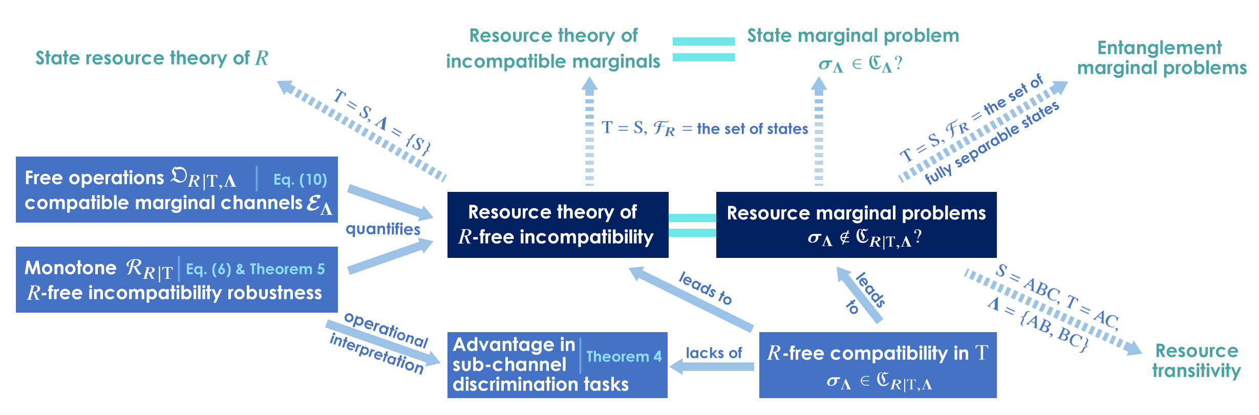
Among others, resource marginal problems contain as special cases the usual marginal problem for quantum states and the problem of deciding whether a given system is a resourceful state. Of course, our unified framework allows us to obtain a general, quantitative analysis beyond these special cases, see Fig. 1. Note further that assuming $\bm{\sigma}_{{\bm{\Lambda}}}\in\mathfrak{C}_{{\bm{\Lambda}}}$ may be very natural, e.g., in the certification of the resource nature of ${\rm T}$. However, this assumption does not have to be imposed a priori since the characterization of $\mathfrak{C}_{{\bm{\Lambda}}}$ represents a specific instance of our general problem. Indeed, checking the membership of $\mathfrak{C}_{{\bm{\Lambda}}}\setminus\mathfrak{C}_{R|{\rm T},{\bm{\Lambda}}}$ is equivalent to determining the membership of both $\mathfrak{C}_{{\bm{\Lambda}}}$ and $\mathfrak{C}_{R|{\rm T},{\bm{\Lambda}}}$. Hence, we shall stick to the most general setting given by the definition of $R$-free compatibility in subsequent discussions.

Figure 1: Summary of the various key notions introduced (boxed) in this work and how they are related to each other. For a given collection of density matrices $\bm{\sigma}_{{\bm{\Lambda}}}$ for subsystems $\bm{\Lambda}$, the set of compatible $\bm{\sigma}_{{\bm{\Lambda}}}$ is denoted by $\mathfrak{C}_{{\bm{\Lambda}}}$. When a resource $R$ and a target subsystem ${\rm T}$ are also specified, one can further define $\mathfrak{C}_{R|{\rm T},{\bm{\Lambda}}}\subseteq\mathfrak{C}_{{\bm{\Lambda}}}$ such that all members of $\mathfrak{C}_{R|{\rm T},{\bm{\Lambda}}}$ are $R$-free compatible in ${\rm T}$. This primitive notion immediately leads to the resource marginal problem corresponding to a given $R$, ${\rm T}$, and $\bm{\sigma}_{{\bm{\Lambda}}}$. When $\bm{\sigma}_{{\bm{\Lambda}}}\in\mathfrak{C}_{R|{\rm T},{\bm{\Lambda}}}$ is taken as a free resource and the set $\mathfrak{O}_{R|{\rm T},\bm{\Lambda}}$ of compatible marginal channels $\mathbfcal{E}_{\bm{\Lambda}}$, Section III.5, is taken as the set of free operations, then we also obtain the resource theory of $R$-free incompatibility. A dashed line originating from a node leads to a special case of this node. Double solid lines without any arrow connecting two nodes means that a one-to-one correspondence can be established between the two.

III.2 $R$-Free Incompatibility As A Resource

Inspired by the approach of Refs. Uola2019 ; Uola2020 , we now introduce the $R$-free incompatibility robustness $\mathcal{R}_{R|{\rm T}}(\bm{\sigma}_{{\bm{\Lambda}}})$ to quantify resource-free incompatibility. Formally, for every set of states $\bm{\sigma}_{{\bm{\Lambda}}}$, define

$$\mathcal{R}_{R|{\rm T}}(\bm{\sigma}_{{\bm{\Lambda}}})\coloneqq$$

$$\quad\inf_{p,\bm{\tau}_{\bm{\Lambda}}}-\log_{2}\left\{0\leq p\leq 1\,|\,p\bm{\sigma}_{{\bm{\Lambda}}}+\left(1-p\right)\bm{\tau}_{\bm{\Lambda}}\in\mathfrak{C}_{R|{\rm T},{\bm{\Lambda}}}\right\}.$$ (6)

Evidently, $\mathcal{R}_{R|{\rm T}}(\bm{\sigma}_{{\bm{\Lambda}}})\geq 0$ and equality holds if and only if $\bm{\sigma}_{{\bm{\Lambda}}}\in\mathfrak{C}_{R|{\rm T},{\bm{\Lambda}}}$. Hence, $\mathcal{R}_{R|{\rm T}}>0$ certifies $R$-free incompatibility. Now, for a given set of operators ${\bf O}_{\bm{\Lambda}}\coloneqq\{O_{\rm X}\}_{\rm X\in{\bm{\Lambda}}}$, we define $\langle\bm{\sigma}_{{\bm{\Lambda}}},{\bf O}_{\bm{\Lambda}}\rangle\coloneqq\sum_{{\rm X\in}\bm{\Lambda}}{\rm tr}(\sigma_{\rm X}O_{\rm X})$. Following the methodologies of Refs. Uola2019 ; Uola2020 ; Takagi2019 , we have the following result, whose proof is given in Appendix D.1.

Theorem 1.

($R$-Free Incompatibility Witness) Let $R$ satisfy the following assumptions:

1. $\mathcal{F}_{R|\rm T}$ is convex and compact.

2. There exists $\rho_{\rm S}$ such that $\rho_{\rm T}\in\mathcal{F}_{R|\rm T}$ and $\rho_{\rm X}$ is full rank for every ${\rm X\in}\bm{\Lambda}$.

Then $\bm{\sigma}_{{\bm{\Lambda}}}\notin\mathfrak{C}_{R|{\rm T},{\bm{\Lambda}}}$ if and only if there exists ${\bf W}_{\bm{\Lambda}}\coloneqq\{W_{\rm X}\succeq 0\}_{{\rm X\in}\bm{\Lambda}}$ such that $\sup_{\bm{\tau}_{\bm{\Lambda}}\in\mathfrak{C}_{R|{\rm T},{\bm{\Lambda}}}}\langle\bm{\tau}_{\bm{\Lambda}},{\bf W}_{\bm{\Lambda}}\rangle<\langle\bm{\sigma}_{{\bm{\Lambda}}},{\bf W}_{\bm{\Lambda}}\rangle.$

Theorem 1 can be understood as the witness of $R$-free incompatibility, i.e., the $R$-free incompatibility of any given $\bm{\sigma}_{{\bm{\Lambda}}}$ can always be detected by a separating hyperplane formed by finitely many positive semi-definite $W_{\rm X}$.

III.3 Robustness Measure As A Conic Program and the Minimal Assumptions For Its Regularity

In Appendix C we show that $2^{\mathcal{R}_{R|{\rm T}}(\bm{\sigma}_{{\bm{\Lambda}}})}$ is the solution of the following optimization problem:

$$\begin{aligned} \min_{V}\quad&{\rm tr}(V)\\ {\rm s.t.}\quad&V\in\mathbfcal{C}_{R|{\rm T}};\;\sigma_{\rm X}\preceq{\rm tr}_{\rm S\setminus X}(V)\quad\forall\;{\rm X\in}{\bm{\Lambda}},\end{aligned}$$ (7a)

where

$$\mathbfcal{C}_{R|{\rm T}}\coloneqq\{\alpha\eta_{\rm S}\,|\,\alpha\geq 0,\eta_{\rm S}:{\rm state\;s.t.}\;{\rm tr}_{\rm S\setminus T}(\eta_{\rm S})\in\mathcal{F}_{R|\rm T}\}.$$ (7b)

This makes it clear that, provided $\mathbfcal{C}_{R|{\rm T}}$ is a proper cone, the computation of $\mathcal{R}_{R|{\rm T}}$ can be cast as a conic program. However, even then, strong duality may not be guaranteed to hold, or $\mathcal{R}_{R|{\rm T}}$ could be unbounded. Next, we present the minimal assumptions required to meet these desirable features.

In Appendix D.2 we prove the following result:

Proposition 2.

(Minimal Assumptions) Given a state resource $R$, the following statements are equivalent:

1. Assumptions (A1) and (A2) from Theorem 1 hold.

2. $\mathbfcal{C}_{R|{\rm T}}$ is a proper cone. Moreover, for every $\bm{\sigma}_{{\bm{\Lambda}}}$, Eq. (7) is a finite conic program with strong duality.

Note that Statement 2 excludes the possibility that the primal and dual optimum coincide at infinite value. Proposition 2 illustrates that Assumptions (A1) and (A2) are both necessary and sufficient for Eq. (7) (and hence $\mathcal{R}_{R|{\rm T}}$) to be a finite conic program with strong duality. Hence, the generality of our approach can be seen from the fact that Assumptions (A1) and (A2) are shared by several common state resource theories (see below the discussions).

Let us now comment on the significance of these assumptions. The convexity of $\mathcal{F}_{R|\rm T}$ in Assumption (A1) implies that probabilistic mixtures of free states is again free. Compactness of $\mathcal{F}_{R|\rm T}$, on the other hand, means that when a state $\rho$ can be approximated by free states with arbitrary precision, then $\rho$ is also free. These features are shared by many resources, such as entanglement, coherence, athermality, asymmetry, steerability, and nonlocality (see Appendix A.5).

However, it is important to remark that not every resource satisfies Assumption (A1). Firstly, convexity implicitly allows shared randomness for free. This is no longer true, for instance, when $\mathcal{F}_{R}$ is the set of multipartite states that are separable with respect to some bipartition. Since a non-trivial convex combination of two states separable in different bipartitions will generally not result in a state separable with respect to any bipartition, $\mathcal{F}_{R}$, and hence $\mathcal{F}_{R|\rm T}$ can be non-convex. Likewise, if one identifies all pure states as the resource, then $\mathcal{F}_{R}$ will be the set of all non-pure states, which is not closed.

Assumption (A2) implies that there exists a free state $\eta_{\rm T}$ in ${\rm T}$ that may be extended to ${\rm S}$ as $\rho_{\rm S}$ such that all the corresponding $\rho_{\rm X}$ are full rank. By considering an extension of the kind $\rho_{\rm S}=\frac{\mathbb{I}_{S\setminus T}}{d_{S\setminus T}}\otimes\eta_{\rm T}$, we see that Assumption (A2) holds whenever the following sufficient condition holds:

1. There exists a full-rank $\eta_{\rm T}\in\mathcal{F}_{R|\rm T}$.

This is, however, not necessary, and a counterexample is given in Appendix D.3. From here we learn that Assumption (A2) is satisfied when a maximally mixed state is a free state. Hence, all but athermality of the above-mentioned resources fulfill this assumption. In the case of athermality, when the given thermal state is full-rank, then this property is again satisfied. This also provides an example where Assumption (A2) becomes invalid, e.g., when the given thermal state is a product pure state, which can be understood as the zero temperature limit without entanglement. From here we also learn that:

Corollary 3.

If Assumptions (A1) and (A2enumi) hold for a given state resource $R$, then $\mathbfcal{C}_{R|{\rm T}}$ is a proper cone. Moreover, for every $\bm{\sigma}_{{\bm{\Lambda}}}$, Eq. (7) is a finite conic program with strong duality.

Figure 2: Schematic illustration of the sub-channel discrimination task. With probability $p_{\rm X}$, the subsystem ${\rm X}\in{\bm{\Lambda}}$ is selected, and one needs to distinguish channels $\{\mathcal{E}_{i|{\rm X}}\}_{i}$ implemented with the probability $\{p_{i|{\rm X}}\}_{i}$. To do so, the local agent prepares the local state $\sigma_{\rm X}$ as the input of the unknown selected channel, and use the POVM $\{E_{i|{\rm X}}\}_{i}$ to measure channel’s output. The agent then guesses the channel is $\mathcal{E}_{j|{\rm X}}$ if the measurement outcome is $j$.

III.4 Operational Interpretation of $R$-Free Incompatibility

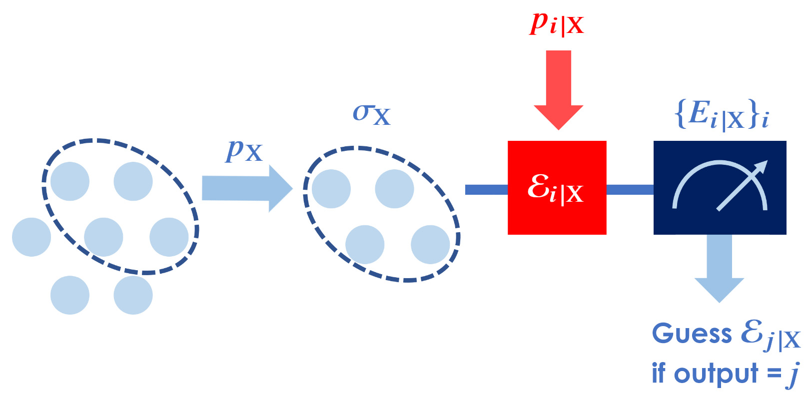
Interestingly, Theorem 1 can be used to construct an operational interpretation that shows how $R$-free incompatibility leads to an advantage in a sub-channel discrimination task, analogous to those discussed in Refs. Takagi2019-2 ; Takagi2019 . For any given $\bm{\sigma}_{{\bm{\Lambda}}}$, let $\mathbfcal{E}\coloneqq\{\mathcal{E}_{i|{\rm X}}\}_{i,{\rm X}}$ be the set of subchannels to be distinguished, then the task consists in the following steps:

1. With probability $p_{\rm X}$, the agent at ${\rm X}\in{\bm{\Lambda}}$ is chosen.

2. With probability $p_{i|{\rm X}}$, the channel $\mathcal{E}_{i|{\rm X}}\in\mathbfcal{E}$ is chosen to be implemented at ${\rm X}$.

3. The agent at ${\rm X}$ inputs the quantum state $\sigma_{\rm X}$ through the channel and applies the positive operator-valued measurements (POVMs) QCI-book $\{E_{i|{\rm X}}\}_{i}$ ($\sum_{i}E_{i|{\rm X}}=\mathbb{I}_{\rm X}$ and $E_{i|{\rm X}}\succeq 0$) to the channel’s output.

4. If the measurement outcome is $j$, the agent guesses $\mathcal{E}_{j|{\rm X}}$ as the channel implemented.

See also Fig. 2 for a schematic illustration of this task. Together, $D\coloneqq\left(\{p_{\rm X}\}_{\rm X},\{p_{i|{\rm X}}\}_{i},\{E_{i|{\rm X}}\}_{i}\right)$ defines the discrimination task. For any chosen input states $\bm{\sigma}_{{\bm{\Lambda}}}=\{\sigma_{\rm X}\}_{{\rm X}\in{\bm{\Lambda}}}$, the probability of successfully distinguish members of $\mathbfcal{E}$ in this task, when averaged over multiple rounds, is evidently

$$P_{D}(\bm{\sigma}_{{\bm{\Lambda}}},\mathbfcal{E})\coloneqq\sum_{{\rm X\in}\bm{\Lambda}}\sum_{i}p_{\rm X}p_{i|{\rm X}}{\rm tr}\left[E_{i|{\rm X}}\mathcal{E}_{i|{\rm X}}(\sigma_{\rm X})\right].$$ (8)

Hereafter, we focus on tasks $D$ that are strictly positive, i.e., $p_{\rm X},p_{i|{\rm X}}>0,E_{i|{\rm X}}\succ 0\;\forall\;i\;\&\;{\rm X}$ and where the ensemble of channels is unitary, i.e., $\mathbfcal{E}=\mathbfcal{U}:=\{\mathcal{U}_{i|{\rm X}}\}_{i,{\rm X}}$ and each $\mathcal{U}_{i|{\rm X}}$ is unitary. Then in Appendix D.4 we show the following:

Theorem 4.

(Advantage in Channel Discrimination) If $R$ satisfies Assumptions (A1) and (A2), then $\bm{\sigma}_{{\bm{\Lambda}}}\notin\mathfrak{C}_{R|{\rm T},{\bm{\Lambda}}}$ if and only if for every unitary $\mathbfcal{U}=\{\mathcal{U}_{i|{\rm X}}\}_{i=1;{\rm X\in\bm{\Lambda}}}^{d_{\rm X}+1}$ there exists a strictly positive subchannel discrimination task $D$ such that $\sup_{\bm{\tau_{\Lambda}}\in\mathfrak{C}_{R|{\rm T},{\bm{\Lambda}}}}P_{D}(\bm{\tau}_{\bm{\Lambda}},\mathbfcal{U})<P_{D}(\bm{\sigma}_{{\bm{\Lambda}}},\mathbfcal{U}).$

Hence, $R$-free incompatibility implies an advantage in distinguishing reversible channels. A few remarks are now in order. Firstly, as the discrimination task is derived from the witness ${\bf W}_{\bm{\Lambda}}$ of Theorem 1, it is specific to the given $\bm{\sigma}_{{\bm{\Lambda}}}$. In general, we should think of the agents somehow having access to $\bm{\sigma}_{{\bm{\Lambda}}}$ and, upon chosen, use the corresponding $\sigma_{\rm X}$ to perform the discrimination task. If $\bm{\sigma}_{{\bm{\Lambda}}}$ is compatible, then these $\sigma_{\rm X}$’s are simply the reduced states of some global state $\rho_{S}$. The resourceful nature of $\rho_{\rm T}$ then guarantees an advantage in the aforementioned discrimination task. Note also that an operational advantage of a wide range of resources in the form of a discrimination task has been discussed, e.g., in Refs. Takagi2019 ; Uola2019 ; Uola2020 . Here, we show that this advantage extends to $R$-free incompatibility and can be manifested by considering a discrimination task that is strictly positive and that involves only unitaries.

III.5 Completing the Resource Theory of $R$-Free Incompatibility

The above observation suggests that $R$-free incompatibility itself is a resource, since it provides advantages in a nontrivial discrimination task that is otherwise absent. Accordingly, the free quantities are simply members of $\mathfrak{C}_{R|{\rm T},{\bm{\Lambda}}}$. To define the free operations, let us first recall the notion of channel compatibility recently introduced in Ref. Hsieh2021 . Throughout, we use $\mathcal{E}_{\rm A\to B}$ to represent a channel mapping from systems ${\rm A}$ to ${\rm B}$. If the input and output Hilbert space are the same, say, both being ${\rm X}$, we further simplify this notation to $\mathcal{E}_{\rm X}$. Then, a global channel $\mathcal{E}_{\rm S^{\prime}\to S}$ mapping from ${\rm S^{\prime}}$ to ${\rm S}$ is said to have a well-defined marginal in the input-output pair ${\rm X^{\prime}\to X}$ (with ${\rm X^{\prime}\subseteq S^{\prime}}$ and ${\rm X\subseteq S}$) if there exists a marginal channel, denoted by $\mathcal{E}_{\rm X^{\prime}\to X}$, from ${\rm X^{\prime}}$ to ${\rm X}$ such that the following commutation relation holds Hsieh2021 :

$${\rm tr}_{\rm S\setminus X}\circ\mathcal{E}_{\rm S^{\prime}\to S}=\mathcal{E}_{\rm X^{\prime}\to X}\circ{\rm tr}_{\rm S^{\prime}\setminus X^{\prime}}.$$ (9)

Once such a marginal exists, it is provably unique Hsieh2021 and we use ${\rm Tr}_{\rm S^{\prime}\setminus X^{\prime}\to S\setminus X}\mathcal{E}_{\rm S^{\prime}\to S}\coloneqq\mathcal{E}_{\rm X^{\prime}\to X}$ to denote the marginal channel of $\mathcal{E}_{\rm S^{\prime}\to S}$ from ${\rm X^{\prime}\to X}$. Notice that, apart from the capitalization in ${\rm Tr}(\cdot)$, the notation for this marginalization operation also differs from the usual partial trace operation ${\rm tr}(\cdot)$ in that the subscripts associated with ${\rm Tr}$ always take the form of “$\cdot\to\cdot$”. For $\mathcal{E}_{\rm S^{\prime}\to S}$, the existence of ${\rm Tr}_{\rm S^{\prime}\setminus X^{\prime}\to S\setminus X}\mathcal{E}_{\rm S^{\prime}\to S}$ is equivalent to being semi-causal in ${\rm X}$ Beckman2001 ; Piani2006 ; Eggeling2002 , semi-localizable in ${\rm X}$ Eggeling2002 , and no-signaling from ${\rm S^{\prime}\setminus X^{\prime}}$ to ${\rm X}$ Duan2016 .

In these terms, we say that a global channel $\mathcal{E}_{{\rm S}}$ on ${\rm S}$ is compatible with a set of channels $\mathbfcal{E}_{\bm{\Lambda}}=\{\mathcal{E}_{\rm X}\}_{{\rm X\in}\bm{\Lambda}}$ acting on subsystem(s) ${\rm X}$ if ${\rm Tr}_{\rm S\setminus X\to S\setminus X}\mathcal{E}_{\rm S}=\mathcal{E}_{\rm X}\;\forall\;{{\rm X\in}\bm{\Lambda}}$. We are now ready to define the free operation of the resource theory associated with $R$-free incompatibility as:

$$\mathfrak{O}_{R|{\rm T},\bm{\Lambda}}\coloneqq$$

$$\{\mathbfcal{E}_{\bm{\Lambda}}\;|\;\exists\;\mathcal{E}_{\rm S}\;{\rm compatible\;with}\;\mathbfcal{E}_{\bm{\Lambda}}\;{\rm s.t.}\;{\rm Tr}_{\rm S\setminus T\to S\setminus T}\mathcal{E}_{\rm S}\in\mathcal{O}_{R}\},$$ (10)

where $\mathcal{O}_{R}$ denotes the set of free operations of the given state resource $R$. Indeed, the legitimacy of this choice follows directly from the definition, i.e., (see Appendix D.5)

$$\mathbfcal{E}_{\bm{\Lambda}}(\bm{\tau}_{\bm{\Lambda}})\in\mathfrak{C}_{R|{\rm T},{\bm{\Lambda}}}\;\forall\;\bm{\tau}_{\bm{\Lambda}}\in\mathfrak{C}_{R|{\rm T},{\bm{\Lambda}}}\text{ and }\forall\;\mathbfcal{E}_{\bm{\Lambda}}\in\mathfrak{O}_{R|{\rm T},\bm{\Lambda}}.$$ (11)

Moreover, as we show in Appendix D.5, $\mathcal{R}_{R|{\rm T}}$ is a monotone with respect to this choice of free operations.

Theorem 5.

($R$-Free Incompatibility Monotone) If $R$ satisfies Assumptions (A1) and (A2), then $\mathcal{R}_{R|{\rm T}}(\bm{\tau}_{\bm{\Lambda}})=0$ if and only if $\bm{\tau}_{\bm{\Lambda}}\in\mathfrak{C}_{R|{\rm T},{\bm{\Lambda}}}$. Moreover, $\mathcal{R}_{R|{\rm T}}\left[\mathbfcal{E}_{\bm{\Lambda}}(\bm{\sigma}_{{\bm{\Lambda}}})\right]\leq\mathcal{R}_{R|{\rm T}}(\bm{\sigma}_{{\bm{\Lambda}}})$ $\forall\;\bm{\sigma}_{{\bm{\Lambda}}},\forall\;\mathbfcal{E}_{\bm{\Lambda}}\in\mathfrak{O}_{R|{\rm T},\bm{\Lambda}}$.

Hence, not only can $\mathcal{R}_{R|{\rm T}}$ quantify $R$-free incompatibility, but it is also a monotone with respect to the judicious choice of free operations given in Section III.5. Together with Theorem 5, we thus complete the resource theory associated with $R$-free incompatibility.

IV Applications and Implications

IV.1 Applications to State Resource Theories and Marginal Problems

We now illustrate the versatility of our framework by considering several explicit examples. By choosing ${\rm T=S}$ and $\bm{\Lambda}=\{{\rm S}\}$, $\mathfrak{C}_{R|{\rm T},{\bm{\Lambda}}}$ and $\mathfrak{O}_{R|{\rm T},\bm{\Lambda}}$ reduce, respectively, to $\mathcal{F}_{R}$ (more precisely, $\mathcal{F}_{R|\rm S}$) and $\mathcal{O}_{R}$. Then, the notion of “$R$-free incompatibility” is exactly the requirement of being $R$-free. Hence, as we illustrate in Fig. 1, the resource theory of $R$-free incompatibility reduces to the resource theory of $R$, and the robustness measure $\mathcal{R}_{R|{\rm T}}$ becomes the one induced by the max-relative entropy Datta2009 . Since these observations hold regardless of the choice of S, we obtain the following application of Theorem 4:

Corollary 6.

Let $\mathcal{F}_{R}$ be convex and compact, $d$ be the dimension of the state space of interest. Suppose there exists a full-rank free state. Then $\rho\notin\mathcal{F}_{R}$ if and only if for every unitary $\mathbfcal{U}=\{\mathcal{U}_{i}\}_{i=1}^{d+1}$ there exists a strictly positive $D$ such that $\max_{\eta\in\mathcal{F}_{R}}P_{D}(\eta,\mathbfcal{U})<P_{D}(\rho,\mathbfcal{U}).$

In contrast with the results previously derived in Refs. Takagi2019-2 ; Takagi2019 , Corollary 6 dictates that an operational advantage in distinguishing subchannels even holds for every combination of unitary channels.

For ${\rm T=S}$ and $\mathcal{F}_{R|\rm S}$ being the set of all states on ${\rm S}$, we have $\mathfrak{C}_{R|{\rm T},{\bm{\Lambda}}}=\mathfrak{C}_{{\bm{\Lambda}}}$, then our resource marginal problem becomes the usual quantum state marginal problem for a given $\bm{\sigma}_{{\bm{\Lambda}}}$. Since all states are “free,” the requirement of “$R$-free compatible” is simply the requirement of marginals compatibility. Then, $R$-free incompatibility reduces to the usual marginal state incompatibility, and the resource theory of $R$-free incompatibility becomes the resource theory of state incompatibility (see Fig. 1). Accordingly, $\mathcal{O}_{R}$ is the set of all channels on ${\rm S}$, $\mathfrak{C}_{R|{\rm T},{\bm{\Lambda}}}=\mathfrak{C}_{{\bm{\Lambda}}}$ is the set of all compatible $\bm{\tau}_{\bm{\Lambda}}$, and $\mathfrak{O}_{R|{\rm T},\bm{\Lambda}}$ is the set of all compatible channels $\mathbfcal{E}_{\bm{\Lambda}}$ acting on ${\rm X}\in{\bm{\Lambda}}$ Hsieh2021 . Moreover, Assumptions (A1) and (A2) are easily verified, thereby giving the following corollary from Theorem 4:

Corollary 7.

$\bm{\sigma}_{{\bm{\Lambda}}}$ is incompatible if and only if for every unitary $\mathbfcal{U}=\{\mathcal{U}_{i|{\rm X}}\}_{i=1;{\rm X\in\bm{\Lambda}}}^{d_{\rm X}+1}$ there exists a strictly positive $D$ such that $\max_{\bm{\tau}_{\bm{\Lambda}}\in\mathfrak{C}_{{\bm{\Lambda}}}}P_{D}(\bm{\tau}_{\bm{\Lambda}},\mathbfcal{U})<P_{D}(\bm{\sigma}_{{\bm{\Lambda}}},\mathbfcal{U}).$

This can be seen as an approach alternative to that provided in Ref. Hall2007 for witnessing the incompatibility of a given $\bm{\sigma}_{{\bm{\Lambda}}}$.

IV.2 Application: Resource Theory Associated with the Entanglement Marginal Problems

As the third application, consider the case of ${\rm T=S}$ and $\mathcal{F}_{R}=$ the set of fully separable states in some given multipartite system ${\rm S}$. For $\bm{\sigma}_{{\bm{\Lambda}}}\in\mathfrak{C}_{{\bm{\Lambda}}}$, this gives exactly the entanglement marginal problem recently proposed in Ref. Navascues2021 , which aims to characterize when a given set of marginal density matrices $\bm{\sigma}_{{\bm{\Lambda}}}$ necessarily implies that the multipartite global state is entangled. By definition, all such entanglement-implying $\bm{\sigma}_{{\bm{\Lambda}}}$ are $R$-free incompatible in the global system ${\rm S}$.

By virtue of Theorem 5, cf. Fig. 1, this incompatibility therefore gives rise to a resource theory defined by the relevant free operations. Since the set $\mathcal{F}_{R}$ is convex and compact, Assumption (A1) holds. Evidently, the maximally mixed state is a member of $\mathcal{F}_{R}$, thus Assumption (A2) is satisfied too. Hence, Theorem 1 guarantees that the incompatibility of any given $\bm{\sigma}_{{\bm{\Lambda}}}$ can always be certified with the help of a certain witness ${\bf W}_{\bm{\Lambda}}$, which admits an operational interpretation (Theorem 4). The robustness measure of Section III.2 can then used to quantify the resourceful nature of $\bm{\sigma}_{{\bm{\Lambda}}}$ within this resource theory of incompatibility.

Note that one may also choose $R=$ genuinely multipartite entanglement, which means that $\mathcal{F}_{R}$ is the convex hull of the union of all biseparable states. Then, as with the original entanglement marginal problems Navascues2021 , marginal states that are only compatible with a genuinely multipartite entangled global state can be treated as a resource, and our framework immediately provides the corresponding resource theory, resource monotone, and its operational interpretation in terms of a subchannel discrimination task.

IV.3 Application to the Transitivity of Quantum Resources

As another example of application, note that our framework provides a natural starting point for the study of the transitivity problem of any given state resource $R$. For simplicity, we illustrate this in a tripartite setting with ${\rm S=ABC}$, $\bm{\Lambda}=\{{\rm AB,BC}\}$, and ${\rm T=AC}$. Inspired by the work of Ref. Coretti2011 , we say that the given resource $R$ is transitive if there exists compatible $\bm{\sigma}_{{\bm{\Lambda}}}=\{\sigma_{\rm AB},\sigma_{\rm BC}\}$ such that $\sigma_{\rm AB},\sigma_{\rm BC}\notin\mathcal{F}_{R}$ and for every $\rho_{\rm S}$ compatible with $\bm{\sigma}_{{\bm{\Lambda}}}$, we have $\rho_{\rm AC}\notin\mathcal{F}_{R}$. In other words, the transitivity of $R$ can be certified by identifying $\bm{\sigma}_{{\bm{\Lambda}}}\in\mathfrak{C}_{{\bm{\Lambda}}}$ such that $\bm{\sigma}_{{\bm{\Lambda}}}\not\in\mathfrak{C}_{R|{\rm T},{\bm{\Lambda}}}$.

An in-depth analysis focusing on entanglement transitivity and related problems can be found in the companion paper Tabia (see also Ref. HsiehRT for a more general discussion involving an arbitrary state resource $R$). Here, we focus on using this specific choice of ${\rm S}$, ${\rm T}$, and $\bm{\Lambda}$ to illustrate the broad applicability of our framework. In particular, for a resource $R$ such that Assumption (A1) and Assumption (A2) hold, a resource theory, in view of Theorem 5, can again be defined for marginals $\bm{\sigma}_{{\bm{\Lambda}}}$ that exhibit resource transitivity. Likewise, a collection of operators ${\bf W}_{\bm{\Lambda}}$ can be used to witness this fact and to demonstrate an advantage in an operational task. The robustness measure of Section III.2 can also be used to quantify the resourcefulness of the given $\bm{\sigma}_{{\bm{\Lambda}}}$.

As a concrete example, consider $\bm{\sigma}_{{\bm{\Lambda}}}=\bm{\sigma}_{{\bm{\Lambda}}}^{W}$ with $\sigma_{\rm AB}=\sigma_{\rm AC}=\sigma^{W}$, where $\sigma^{W}$ is the bipartite marginal of the three-qubit $W$-state Dur2000 $|W_{\rm ABC}\rangle\coloneqq\frac{1}{\sqrt{3}}\left(|001\rangle+|010\rangle+|100\rangle\right)_{\rm ABC}$. It is known wu2014 that the only three-qubit state compatible with this given $\bm{\sigma}_{{\bm{\Lambda}}}$ is the $W$-state itself, and hence the $AC$ marginal must also be $\sigma^{W}$, thereby showing the transitivity of entanglement.

To illustrate the advantage alluded to in Theorem 4, we consider a discrimination task $D^{\mathbfcal{U}}\coloneqq\left(\{p_{\rm X},p_{i|{\rm X}}\},\{E{U}_{i|{\rm X}}\}\right)$ with $p_{\rm X}=\frac{1}{2}$, $p_{i|{\rm X}}=\frac{0.99}{4},i=1,2,3,4$ and $p_{5|{\rm X}}=0.01$ for both ${\rm X=AB,BC}$, and the POVM elements $E_{i|{\rm X}}$ specified in Appendix D.7. Then, for $N=10^{5}$ sets of five unitary matrices $\mathbfcal{U}=\{U_{i|{\rm X}}\}_{i=1;{\rm X}\in\bm{\Lambda}}^{5}$, each randomly generated according to the Haar measure, we compute the operational advantage $\Delta P=P_{D}(\bm{\sigma}_{{\bm{\Lambda}}},\mathbfcal{U})-\max_{\bm{\tau}_{\bm{\Lambda}}\in\mathfrak{C}_{R|{\rm T},{\bm{\Lambda}}}}P_{D}(\bm{\tau}_{\bm{\Lambda}},\mathbfcal{U})$ where $\mathfrak{C}_{R|{\rm T},{\bm{\Lambda}}}$ is the set of $\bm{\sigma}_{{\bm{\Lambda}}}$ giving rise to a separable two-qubit state in AC. A histogram of the results obtained, see Fig. 3, clearly demonstrates the said advantage mentioned in Theorem 4.

We conclude this section by noting that together with the results established in Refs. Palazuelos2012 ; Cavalcanti2013 , the entanglement transitivity of $\bm{\sigma}_{{\bm{\Lambda}}}^{W}$ implies the transitivity of nonlocality, and hence the steerability (see also Refs. Hsieh2016 ; Quintino2016 ) of multiple copies of these marginals. We shall refer to this phenomenon as weak nonlocality transitivity, which is formalized as follows.

Theorem 8.

(Weak Nonlocality Transitivity) For every integer $k$ larger than some finite threshold value $k_{c}$, there exist nonlocal $\sigma_{\rm AB},\sigma_{\rm BC}$ such that for every $\rho_{\rm ABC}\in\mathcal{S}\left[(\mathbb{C}^{2})^{\otimes k}\otimes(\mathbb{C}^{2})^{\otimes k}\otimes(\mathbb{C}^{2})^{\otimes k}\right]$ compatible with them, the corresponding $\rho_{\rm AC}$ must be nonlocal.

Here, we use $\mathcal{S}\left[(\mathbb{C}^{2})^{\otimes k}\otimes(\mathbb{C}^{2})^{\otimes k}\otimes(\mathbb{C}^{2})^{\otimes k}\right]$ to refer to the set of $3k$-qubit density matrices where ${\rm A},{\rm B}$, and ${\rm C}$ holds $k$-qubit each. For a proof of the Theorem, we refer the readers to Appendix D.8 (see also Ref. Tabia ). Importantly, Theorem 8 gives the first example of nonlocality (and hence also steerability) transitivity for quantum states, albeit under the auxiliary assumption that the global state admits the aforementioned tensor-product structure. Prior to the present work, transitivity of nonlocality is only known to exist at the level of no-signaling correlations Coretti2011 that do not admit a quantum representation.

Figure 3: Histogram of the operational advantage $\Delta P$ derived from $\bm{\sigma}_{{\bm{\Lambda}}}^{W}$ in a series of $N=10^{5}$ sub-channel discrimination tasks involving unitary sub-channels randomly chosen according to the Haar measure. With bin widths of size $10^{-4}$, our data has the smallest and the largest $\Delta P$ of $0.001884$ and $0.010274$, respectively. It also has a mean and standard deviation of $0.0066818\pm 0.0012439$.

V Discussion

Motivated by the importance and the generality of quantum states marginal problems as well as resource theories, we provide an overarching framework that includes not only these two important topics in quantum information theory, but also a variety of other unexplored possibilities. The key notion underlying our framework is resource-free ($R$-free) incompatibility in a target subsystem ${\rm T}$, i.e., the impossibility of having a resource-free subsystem ${\rm T}$ for some given set of marginal states $\bm{\sigma}_{{\bm{\Lambda}}}$. The question of whether this impossibility holds for any given $\bm{\sigma}_{{\bm{\Lambda}}}$ leads naturally to what we dub the resource marginal problems, which includes the quantum state marginal problems as a special case.

To quantify this incompatibility, we introduce a robustness measure $\mathcal{R}_{R|{\rm T}}(\bm{\sigma}_{{\bm{\Lambda}}})$ and show that, provided two necessary and sufficient conditions are satisfied, $\mathcal{R}_{R|{\rm T}}(\bm{\sigma}_{{\bm{\Lambda}}})$ can be evaluated as a finite-valued conic program where strong duality holds. Whenever $\bm{\sigma}_{{\bm{\Lambda}}}$ is not $R$-free compatible, we demonstrate how a witness can be extracted from the conic program to manifest this fact. Moreover, a subchannel discrimination task involving arbitrary unitary channels can be defined to illustrate the operational advantage of $R$-free incompatible $\bm{\sigma}_{{\bm{\Lambda}}}$ over those compatible ones in this task. By identifying appropriate free operations, we further prove that a resource theory of $R$-free incompatibility can be formulated with the robustness measure $\mathcal{R}_{R|{\rm T}}(\bm{\sigma}_{{\bm{\Lambda}}})$ serving as the corresponding monotone. The corresponding resource theory for $R$ is then recovered as a special case of our resource theory.

Apart from recovering the known results, our framework makes evident the fact that an incompatibility problem can be defined for any resource theory for quantum states, and vice versa. For example, a resource theory can be defined for the usual quantum states marginal problems, an incompatibility problem can be defined for the resource theory of entanglement, and so on. In particular, since a resource theory of entanglement-free incompatibility can be defined in relation to the recently introduced entanglement marginal problems Navascues2021 , our robustness measure, etc., can be applied to this incompatibility. More generally, if a resource theory or a marginal problem can be cast in a form that fits our framework, results that we have derived are readily applicable. As a side result that stems from our investigation, we provide the first example demonstrating the transitivity of nonlocality (and steerability) for quantum states under the auxiliary assumption of a tensor-product structure of the underlying state.

Let us conclude by naming some further possibilities for future work. First, as is now well known, not only can resource theories be defined for quantum states, but also for quantum channels (see, e.g., Refs. Uola2020 ; Pirandola2017 ; Hsieh2017 ; Bu2020 ; Diaz2018 ; Rosset2018 ; Wilde2018 ; Bauml2019 ; Seddon2019 ; LiuWinter2019 ; LiuYuan2019 ; Gour2019-3 ; Gour2019 ; Gour2019-2 ; Gour2020-1 ; Takagi2019-3 ; Theurer2019 ; Saxena2019 ; Hsieh2020-2 ; Hsieh2020-3 ; Hsieh2021 ; Hsieh2022 ). By following a treatment very similar to that carried out in this work, we also establish the dynamical analogs of many of the results mentioned above. In the dynamical regime, it would be interesting to see how our framework can be used to obtain further insights in related problems such as channel broadcasting, measurement incompatibility, causal structures, channel extendibility, etc. We refer the reader to the follow-up paper Ref. HsiehDRMP , which lies outside the scope of the present work. Also, with our framework, existing results from various works, including those in Refs. Hall2007 ; Takagi2019-2 ; Takagi2019 ; Uola2019 ; Uola2020 can be recovered. But given the versatility of resource marginal problems, it should be clear that there remain many other possibilities that are worth exploring beyond those explicitly discussed here that are worth further explorations. For example, for the problem of the transitivity of nonlocal states, it will also be highly desirable to see if an example can be provided that does not require the auxiliary assumption that we invoke here.

Appendix A Preliminary Notions: Topological Properties

In this section, we briefly discuss various topological properties of $\mathfrak{C}_{R|{\rm T},{\bm{\Lambda}}}$, $\mathbfcal{C}_{R|{\rm T}}$, and their alternative forms. To keep the clarity of presentation, some new notations are introduced in Section A.1. For convenience, we summarize results relevant to the proofs in later sections in Theorem A.1. After that, Section A.2 discusses convexity, Section A.3 is for a generalized notion of interior, and Section A.4 is for compactness and closedness. Finally, in Section A.5 we briefly discuss the validity of Assumption  (A1) for several state resources by showing the compactness of $\mathcal{F}_{R}$.

A.1 Notations

To start with, we clarify the notations. With a given global system ${\rm S}$ and a set of local systems $\bm{\Lambda}$, we define

$$\mathfrak{C}_{{\bm{\Lambda}}}\coloneqq\{\bm{\sigma}_{{\bm{\Lambda}}}\,|\,\exists\;\rho_{\rm S}\;{\rm s.t.}\;\sigma_{\rm X}=\rho_{\rm X}\;\forall\;{\rm X\in}\bm{\Lambda}\},$$ (12)

which is the set of all compatible $\bm{\sigma}_{{\bm{\Lambda}}}$. Here we adopt the notation $\rho_{\rm X}\coloneqq{\rm tr}_{\rm S\setminus X}(\rho_{\rm S})$. The set of all quantum states on ${\rm S}$ is denoted by

$$\mathcal{S}_{\rm S}\coloneqq\{\rho_{\rm S}\,|\,\rho_{\rm S}\succeq 0,{\rm tr}(\rho_{\rm S})=1\}.$$ (13)

For the convenience of subsequent discussions, we define

$$\mathcal{S}_{{R|{\rm T}}}\coloneqq\left\{\rho_{\rm S}\,|\,\rho_{\rm S}\in\mathcal{S}_{\rm S},\rho_{\rm T}\in\mathcal{F}_{R|{\rm T}}\right\},$$ (14)

which is a set of global states with free marginals in the target system ${\rm T}$. Moreover, for a given set $Q\subseteq\mathcal{S}_{\rm S}$, let the unnormalized versions of $Q$, i.e., the cone corresponding to $Q$, be:

$$\mathcal{C}_{Q}\coloneqq\{\alpha\rho_{\rm S}\,|\,\alpha\geq 0,\rho_{\rm S}\in Q\}.$$ (15)

Then, Eq. (7b) can be rewritten as

$$\mathbfcal{C}_{R|{\rm T}} \coloneqq\{\alpha\rho_{\rm S}\,|\,\alpha\geq 0,\rho_{\rm S}\in\mathcal{S}_{\rm S},\rho_{\rm T}\in\mathcal{F}_{R|{\rm T}}\}$$

$$=\{\alpha\rho_{\rm S}\,|\,\alpha\geq 0,\rho_{\rm S}\in\mathcal{S}_{{R|{\rm T}}}\}=\mathcal{C}_{\mathcal{S}_{R|{\rm T}}}.$$ (16)

In these notations, we have $\mathcal{F}_{R|{\rm T}}=\mathcal{F}_{R}\cap\mathcal{S}_{\rm T}$. For convenience, we first list important observations needed for subsequent proofs below. Recall that a cone $\mathcal{C}$ is pointed if $x\in\mathcal{C}$ and $-x\in\mathcal{C}$ imply $x=0$; it is proper if it is nonempty, convex, compact, and pointed.

Theorem A.1.

Given a state resource $R$, then

1. $\mathcal{F}_{R|{\rm T}}$ is convex and compact implies that $\mathfrak{C}_{R|{\rm T}}$ is convex and compact.

2. $\mathcal{F}_{R|{\rm T}}$ is nonempty, convex, and compact if and only if $\mathbfcal{C}_{R|{\rm T}}$ is a proper cone.

The first statement is a combination of Lemma A.2 and Lemma A.7, and the second statement is a combination of Lemma A.2 and Lemma A.6, and the fact that $\mathbfcal{C}_{R|{\rm T}}$ is by definition pointed; namely, when we have an element $x\in\mathbfcal{C}_{R|{\rm T}}$ such that $-x\in\mathbfcal{C}_{R|{\rm T}}$, then we must have $x=0$, since we must have $x\geq 0$ and $x\leq 0$ simultaneously.

Finally, before starting the discussions, we implicitly assume that ${\rm S},\bm{\Lambda},{\rm T}$ are all given and fixed.

A.2 Convexity

We begin with the following facts regarding convexity:

Lemma A.2.

The following statements are equivalent:

1. $\mathcal{F}_{R|{\rm T}}$ is convex.

2. $\mathfrak{C}_{R|{\rm T},{\bm{\Lambda}}}$ is convex.

3. $\mathcal{S}_{R|{\rm T}}$ is convex.

4. $\mathbfcal{C}_{R|{\rm T}}$ is convex.

Proof.

We will show the following loop: Statements 1 $\Rightarrow$ Statements 2 $\Rightarrow$ Statement 1 $\Rightarrow$ Statement 3 $\Rightarrow$ Statement 4 $\Rightarrow$ Statement 3 $\Rightarrow$ Statement 1.

Statement 1 $\Rightarrow$ Statement 2.– Let $\bm{\sigma}_{{\bm{\Lambda}}},\bm{\tau}_{\bm{\Lambda}}\in\mathfrak{C}_{R|{\rm T},{\bm{\Lambda}}}$ and $p\in[0,1]$, then there exist global states $\rho_{\rm S},\eta_{\rm S}$ compatible with $\bm{\sigma}_{{\bm{\Lambda}}},\bm{\tau}_{\bm{\Lambda}}$, respectively, such that $\rho_{\rm T},\eta_{\rm T}$ are both in $\mathcal{F}_{R|{\rm T}}$. Because $\mathcal{F}_{R|{\rm T}}$ is convex, the convex mixture of $\rho_{\rm S}$ and $\eta_{\rm S}$ satisfies ${\rm tr}_{\rm S\setminus T}\left[p\rho_{\rm S}+(1-p)\eta_{\rm S}\right]=p\rho_{\rm T}+(1-p)\eta_{\rm T}\in\mathcal{F}_{R|{\rm T}}$. On the other hand, we have

$$p\bm{\sigma}_{{\bm{\Lambda}}}+(1-p)\bm{\tau}_{\bm{\Lambda}} =\{p\sigma_{\rm X}+(1-p)\tau_{\rm X}\}_{{\rm X\in}\bm{\Lambda}}$$

$$=\{{\rm tr}_{\rm S\setminus X}\left[p\rho_{\rm S}+(1-p)\eta_{\rm S}\right]\}_{{\rm X\in}\bm{\Lambda}},$$ (17)

meaning that $p\rho_{\rm S}+(1-p)\eta_{\rm S}$ is compatible with $p\bm{\sigma}_{{\bm{\Lambda}}}+(1-p)\bm{\tau}_{\bm{\Lambda}}$. Hence, $p\bm{\sigma}_{{\bm{\Lambda}}}+(1-p)\bm{\tau}_{\bm{\Lambda}}\in\mathfrak{C}_{R|{\rm T},{\bm{\Lambda}}}$, demonstrating the convexity of $\mathfrak{C}_{R|{\rm T},{\bm{\Lambda}}}$.

Statement 2 $\Rightarrow$ Statement 1.– Suppose $\mathfrak{C}_{R|{\rm T},{\bm{\Lambda}}}$ is convex, whose definition is given in Eq. (5). Consider two arbitrary $\rho_{\rm T},\eta_{\rm T}\in\mathcal{F}_{R|{\rm T}}$. Then we have

$$\{{\rm tr}_{\rm S\setminus X}(\zeta_{\rm S\setminus T}\otimes\rho_{\rm T})\}_{{\rm X\in}\bm{\Lambda}}\in\mathfrak{C}_{R|{\rm T},{\bm{\Lambda}}};$$ (18a)

$$\{{\rm tr}_{\rm S\setminus X}(\zeta_{\rm S\setminus T}\otimes\eta_{\rm T})\}_{{\rm X\in}\bm{\Lambda}}\in\mathfrak{C}_{R|{\rm T},{\bm{\Lambda}}},$$ (18b)

where $\zeta_{\rm S\setminus T}$ is an arbitrary state in ${\rm S\setminus T}$. Since $\mathfrak{C}_{R|{\rm T},{\bm{\Lambda}}}$ is convex, we have that, for every $p\in[0,1]$,

$$\{p{\rm tr}_{\rm S\setminus X}(\zeta_{\rm S\setminus T}\otimes\rho_{\rm T})+(1-p){\rm tr}_{\rm S\setminus X}(\zeta_{\rm S\setminus T}\otimes\eta_{\rm T})\}_{{\rm X\in}\bm{\Lambda}}$$

$$=\{{\rm tr}_{\rm S\setminus X}\left(\zeta_{\rm S\setminus T}\otimes\left[p\rho_{\rm T}+(1-p)\eta_{\rm T}\right]\right)\}_{{\rm X\in}\bm{\Lambda}}\in\mathfrak{C}_{R|{\rm T},{\bm{\Lambda}}},$$ (19)

which means $p\rho_{\rm T}+(1-p)\eta_{\rm T}\in\mathcal{F}_{R|{\rm T}}$. This implies the convexity of $\mathcal{F}_{R|{\rm T}}$.

Statement 1 $\Rightarrow$ Statement 3.– Suppose $\mathcal{F}_{R|{\rm T}}$ is convex, then for every $\rho_{\rm S},\eta_{\rm S}\in\mathcal{S}_{R|{\rm T}}$ and $p\in[0,1]$, we have

$${\rm tr}_{\rm S\setminus T}\left[p\rho_{\rm S}+(1-p)\eta_{\rm S}\right]=p\rho_{\rm T}+(1-p)\eta_{\rm T}\in\mathcal{F}_{R|{\rm T}}.$$ (20)

This implies that $p\rho_{\rm S}+(1-p)\eta_{\rm S}\in\mathcal{S}_{R|{\rm T}}$.

Statement 3 $\Rightarrow$ Statement 4.– Consider arbitrary $\alpha\rho_{\rm S},\beta\eta_{\rm S}\in\mathbfcal{C}_{R|{\rm T}}$ with values $\alpha,\beta\geq 0$, states $\rho_{\rm S},\eta_{\rm S}\in\mathcal{S}_{R|{\rm T}}$, and probability $p\in[0,1]$. Then we can write $p\alpha\rho_{\rm S}+(1-p)\beta\eta_{\rm S}=\left[p\alpha+(1-p)\beta\right]\times\left[q\rho_{\rm S}+(1-q)\eta_{\rm S}\right]$, where $q\coloneqq\frac{p\alpha}{p\alpha+(1-p)\beta}\in[0,1]$. By the assumed convexity of $\mathcal{S}_{{R|{\rm T}}}$, $q\rho_{\rm S}+(1-q)\eta_{\rm S}\in\mathcal{S}_{R|{\rm T}}$, which further means that the above quantity is in $\mathbfcal{C}_{R|{\rm T}}$ since $p\alpha+(1-p)\beta\geq 0$. From here we conclude the convexity of $\mathbfcal{C}_{R|{\rm T}}$.

Statement 4 $\Rightarrow$ Statement 3.– Given the convexity of $\mathbfcal{C}_{R|{\rm T}}$, it means the convexity of the set by setting $\alpha=1$; namely, $\{\rho_{\rm S}\,|\,\rho_{\rm S}\in\mathcal{S}_{R|{\rm T}}\}$. Since this set is exactly $\mathcal{S}_{R|{\rm T}}$, the result follows.

Statement 3 $\Rightarrow$ Statement 1.– Assume $\mathcal{S}_{R|{\rm T}}$ is convex. For every $\rho_{\rm T},\eta_{\rm T}\in\mathcal{F}_{R|{\rm T}}$ and $p\in[0,1]$, one can pick an arbitrary state $\zeta_{\rm S\setminus T}$ in ${\rm S\setminus T}$. Then $\zeta_{\rm S\setminus T}\otimes\rho_{\rm T},\zeta_{\rm S\setminus T}\otimes\eta_{\rm T}\in\mathcal{S}_{R|{\rm T}}$, meaning that $\zeta_{\rm S\setminus T}\otimes\left[p\rho_{\rm T}+(1-p)\eta_{\rm T}\right]\in\mathcal{S}_{R|{\rm T}}$. Hence, by definition of $\mathcal{S}_{R|{\rm T}}$, we learn that $p\rho_{\rm T}+(1-p)\eta_{\rm T}\in\mathcal{F}_{R|{\rm T}}$. ∎

A.3 Relative Interior

In order to apply conic programming, it is necessary to understand the property of interior defined in a suitable form. Formally, for a set $Q\subseteq\mathbb{R}^{N}$ with a given $N\in\mathbb{N}$, its relative interior is defined by (see, e.g., Refs. LectureNote ; Bertsekas-book )

$${\rm relint}(Q)\coloneqq\left\{x\in Q\,|\,\exists\,\epsilon>0\;{\rm s.t.}\;\mathcal{B}(x;\epsilon)\cap{\rm aff}(Q)\subseteq Q\right\},$$ (21)

where $\mathcal{B}(x;\epsilon)\coloneqq\{y\in\mathbb{R}^{N}\,|\,\left\|x-y\right\|<\epsilon\}$ is an open ball centering at $x$ with radius $\epsilon$ induced by the usual distance for vectors $\left\|\cdot\right\|$ (note that one can also choose it as one norm or sup norm, since they induce the same topology), and ${\rm aff}(Q)$ is the affine hull of $Q$ LectureNote ; Bertsekas-book . When $Q$ is convex, its relative interior is also given by LectureNote ; Bertsekas-book

$${\rm relint}(Q)\coloneqq\left\{x\in Q\;|\;\forall\,y\in Q,\exists\,l>1\;{\rm s.t.}\;lx+(1-l)y\in Q\right\}.$$ (22)

Let $l=\frac{1}{p}$ for some $p\in(0,1)$, the definition is equivalent to

$${\rm relint}(Q)=$$

$$\{x\in V\;|\;\forall\,y\in Q,\exists\,p\in(0,1)\;\&\;z\in Q\;{\rm s.t.}\;x=pz+(1-p)y\}.$$ (23)

In other words, $x$ can be written as a “strict” convex combination of two members in $Q$. Now we note that:

Lemma A.3.

Given a nonempty convex set $Q\subseteq\mathcal{S}_{\rm S}$. If $\eta_{\rm S}\in{\rm relint}(Q)$, then $\alpha\eta_{\rm S}\in{\rm relint}(\mathcal{C}_{Q})$ for every $\alpha>0$.

Proof.

Given $\alpha>0$ and $\eta_{\rm S}\in{\rm relint}(Q)$. Consider an arbitrarily given $y\in\mathcal{C}_{Q}$, which can be written as $y=\beta\phi_{\rm S}$ for some $\beta\geq 0$ and $\phi_{\rm S}\in Q$ according to its definition Eq. (15). The goal is to show that one can always find some $q\in(0,1)$ and $z\in\mathcal{C}_{Q}$ such that $\alpha\eta_{\rm S}=qy+(1-q)z$, and then use Eq. (A.3) to conclude the desired claim. Now, since $\eta_{\rm S}\in{\rm relint}(Q)$, there exists $\gamma_{\rm S}\in Q$ and $p\in(0,1)$ such that

$$\alpha\eta_{\rm S}=\alpha\left[(1-p)\gamma_{\rm S}+p\phi_{\rm S}\right]=(1-p)\alpha\gamma_{\rm S}+\frac{p\alpha}{\beta}\times\beta\phi_{\rm S},$$ (24)

where the first equality follows from Eq. (A.3). In the second equality, we assume $\beta>0$, since when $\beta=0$, one has $\alpha\eta_{\rm S}=p\times\frac{\alpha\eta_{\rm S}}{p}+(1-p)\times 0$ for every $p\in(0,1)$, where $\frac{\alpha\eta_{\rm S}}{p}\in\mathcal{C}_{Q}$. Now, define the quantity

$$q\coloneqq\begin{cases}\frac{p\alpha}{\beta}\;&{\rm if}\;\frac{p\alpha}{\beta}<1;\\ \frac{1}{2}\;&{\rm if}\;\frac{p\alpha}{\beta}\geq 1.\end{cases}$$ (25)

Note that $\frac{p\alpha}{\beta}>0$ since $p,\beta,\alpha>0$. Then $q\in(0,1)$ and we have

$$\alpha\eta_{\rm S} =(1-q)\times\frac{(1-p)\alpha\gamma_{\rm S}+\left(\frac{p\alpha}{\beta}-q\right)\beta\phi_{\rm S}}{1-q}+q\beta\phi_{\rm S}$$

$$=(1-q)\left(l_{*}\gamma_{\rm S}+k_{*}\phi_{\rm S}\right)+q\beta\phi_{\rm S},$$ (26)

where we define $l_{*}\coloneqq\frac{1-p}{1-q}\times\alpha\geq 0$ and $k_{*}\coloneqq\frac{\beta}{1-q}\times\left(\frac{p\alpha}{\beta}-q\right)\geq 0$, both are non-negative. Finally, write $p_{*}=\frac{l_{*}}{l_{*}+k_{*}}$, then we have $\alpha\eta_{\rm S}=(1-q)\times(l_{*}+k_{*})\times\left[p_{*}\gamma_{\rm S}+(1-p_{*})\phi_{\rm S}\right]+q\beta\phi_{\rm S},$ where $p_{*}\gamma_{\rm S}+(1-p_{*})\phi_{\rm S}\in Q$ since $Q$ is convex and $\gamma_{\rm S},\phi_{\rm S}\in Q$. Due to $l_{*}+k_{*}\geq 0$, we conclude that $(l_{*}+k_{*})\times\left[p_{*}\gamma+(1-p_{*})\phi\right]\in\mathcal{C}_{Q}$. This implies the desired claim; that is, $\alpha\eta_{\rm S}\in{\rm relint}(\mathcal{C}_{Q})$. ∎

A.4 Compactness and Closedness

From now on the topology defined for states will be understood as the one induced by the trace norm $\left\|\cdot\right\|_{1}$. Also, to talk about topology of sets of states $\bm{\sigma}$, we consider the distance measure

$$\left\|\bm{\sigma}-\bm{\tau}\right\|\coloneqq\sum_{\rm X\in{\bm{\Lambda}}}\left\|\sigma_{\rm X}-\tau_{\rm X}\right\|_{1}.$$ (27)

One can check that this gives a metric, since the triangle inequality of Eq. (27) directly follows the triangle inequality of $\left\|\cdot\right\|_{1}$ QCI-book . In what follows, the topological properties are understood as induced by this norm. For the clarity of the proof, the data-processing inequality of $\left\|\cdot\right\|_{1}$ reads

$$\left\|\mathcal{E}(\rho)-\mathcal{E}(\sigma)\right\|_{1}\leq\left\|\rho-\sigma\right\|_{1}\quad\forall\;\mathcal{E}:{\rm channel}.$$ (28)

Conceptually, it means that after a processing channel, two information carriers can only be less distinguishable.

Now we start with the following fact, which means that $\mathcal{C}_{Q}$ defined in Eq. (15) inherits closedness from $Q$.

Lemma A.4.

A given set $Q\subseteq\mathcal{S}_{\rm S}$ is compact if and only if $\mathcal{C}_{Q}$ is closed.

Proof.

We first show the necessity, and then we will prove the sufficiency.

“$\Leftarrow$” direction.– If $\mathcal{C}_{Q}$ is closed, then $Q=\mathcal{C}_{Q}\cap\mathcal{S}_{\rm S}$ is also closed (both are treated as subsets of the space of linear operators acting on a finite-dimensional system ${\rm S}$). The compactness of $Q$ follows from the fact that it is bounded in a finite-dimensional space.

“$\Rightarrow$” direction.– We prove the claim by showing that $\mathcal{C}_{Q}$ will contain all its limit points. To start with, consider a given limit point $\zeta\notin\mathcal{C}_{Q}$ [note that it has a non-zero finite trace $|{\rm tr}(\zeta)|\in(0,\infty)$, since ${\rm tr}(\zeta)=0$ implies that $\zeta=0\in\mathcal{C}_{Q}$]. Then there exists a sequence $\{\alpha_{k}\eta^{(k)}_{\rm S}\}_{k=1}^{\infty}\subseteq\mathcal{C}_{Q}$ with $\alpha_{k}\geq 0,\eta^{(k)}_{\rm S}\in Q\;\forall\;k$ such that $\lim_{k\to\infty}\left\|\zeta-\alpha_{k}\eta^{(k)}_{\rm S}\right\|_{1}=0.$ Using data processing inequality of $\left\|\cdot\right\|_{1}$ [Eq. (28)] under the channel ${\rm tr}(\cdot)$, we learn that $\lim_{k\to\infty}|{\rm tr}(\zeta)-\alpha_{k}|=0.$ In particular, this means that ${\rm tr}(\zeta)$ is an adherent point of the closed set ${\rm tr}(\mathcal{C}_{Q})=[0,\infty)$, which further implies that ${\rm tr}(\zeta)>0$. This means that we can assume $\alpha_{k}>0\;\forall\;k$. Now, for every $0<\epsilon<{\rm tr}(\zeta)$, there exist $n_{1},n_{2}\in\mathbb{N}$ such that

$$\left\|\zeta-\alpha_{k}\eta^{(k)}_{\rm S}\right\|_{1}<\epsilon\quad{\rm if}\;k\geq n_{1};$$ (29a)

$$|{\rm tr}(\zeta)-\alpha_{k}|<\epsilon\quad{\rm if}\;k\geq n_{2}.$$ (29b)

From here we learn that, for every $k\geq\max\{n_{1},n_{2}\}$,

$$\left\|\frac{\zeta}{{\rm tr}(\zeta)}-\eta^{(k)}_{\rm S}\right\|_{1} \leq\left\|\frac{\zeta}{{\rm tr}(\zeta)}-\frac{\zeta}{\alpha_{k}}\right\|_{1}+\left\|\frac{\zeta}{\alpha_{k}}-\eta^{(k)}_{\rm S}\right\|_{1}$$

$$=\left\|\zeta\right\|_{1}\times\frac{|{\rm tr}(\zeta)-\alpha_{k}|}{{\rm tr}(\zeta)\alpha_{k}}+\frac{1}{\alpha_{k}}\times\left\|\zeta-\alpha_{k}\eta^{(k)}_{\rm S}\right\|_{1}$$

$$<\left(\frac{\left\|\zeta\right\|_{1}}{{\rm tr}(\zeta)}+1\right)\times\frac{\epsilon}{\alpha_{k}}$$

$$<\left(\frac{\left\|\zeta\right\|_{1}}{{\rm tr}(\zeta)}+1\right)\times\frac{\epsilon}{{\rm tr}(\zeta)-\epsilon}.$$ (30)

The first line follows from the triangle inequality of $\left\|\cdot\right\|_{1}$ QCI-book and we note that $0<{\rm tr}(\zeta)-\epsilon<\alpha_{k}\;\forall\;k\geq n_{2}$. This implies that $\lim_{k\to\infty}\left\|\frac{\zeta}{{\rm tr}(\zeta)}-\eta^{(k)}_{\rm S}\right\|_{1}=0.$ In other words, $\frac{\zeta}{{\rm tr}(\zeta)}$ is inside the closure of $Q$. Since $Q$ is closed, we learn that $\frac{\zeta}{{\rm tr}(\zeta)}\in Q$. Finally, by writing $\zeta={\rm tr}(\zeta)\times\frac{\zeta}{{\rm tr}(\zeta)}$ and note that ${\rm tr}(\zeta)>0$, we conclude that $\zeta\in\mathcal{C}_{Q}$. Hence, $\mathcal{C}_{Q}$ contains all its limit points, and the proof is completed. ∎

Now we note the following fact:

Lemma A.5.

$\mathfrak{C}_{\bm{\Lambda}}$, $\mathcal{S}_{\rm S}$, and $\mathcal{S}_{\rm S|pure}$ are compact, where $\mathcal{S}_{\rm S|pure}$ is the set of all pure states in ${\rm S}$.

Proof.

[Recall from Eqs. (12) and (13) for the definitions]

Proof of Compactness of $\mathfrak{C}_{\bm{\Lambda}}$.– Define the map

$$f(\rho_{\rm S})\coloneqq\{{\rm tr}_{\rm S\setminus X}(\rho_{\rm S})\}_{{\rm X}\in{\bm{\Lambda}}}.$$ (31)

Then one can observe that $f(\mathcal{S}_{\rm S})=\mathfrak{C}_{\bm{\Lambda}}$, where recall from Eq. (13) that $\mathcal{S}_{\rm S}\coloneqq\{\rho_{\rm S}\,|\,\rho_{\rm S}\succeq 0,{\rm tr}(\rho_{\rm S})=1\}$ is the set of quantum states in ${\rm S}$. Equipping the domain with $\left\|\cdot\right\|_{1}$ and the image with $\left\|\cdot\right\|$ defined in Eq. (27), we learn that

$$\left\|f(\rho_{\rm S})-f(\eta_{\rm S})\right\| =\sum_{\rm X\in{\bm{\Lambda}}}\left\|{\rm tr}_{\rm S\setminus X}(\rho_{\rm S})-{\rm tr}_{\rm S\setminus X}(\eta_{\rm S})\right\|_{1}$$

$$\leq|{\bm{\Lambda}}|\left\|\rho_{\rm S}-\eta_{\rm S}\right\|_{1},$$ (32)

where the inequality follows from the data-processing inequality of $\left\|\cdot\right\|_{1}$ given in Eq. (28). This means that $f$ is continuous, and the result follows by combining the compactness of $\mathcal{S}_{\rm S}$ and the fact that a continuous function maps a compact set to a compact set (see, e.g., Ref. Apostol-book ; Munkres-book ).

Proof of Compactness of $\mathcal{S}_{\rm S}$.– Since $\mathcal{S}_{\rm S}=\{\rho_{\rm S}\,|\,\rho_{\rm S}\succeq 0\}\cap\{\rho_{\rm S}\,|\,{\rm tr}(\rho_{\rm S})=1\}$ and ${\rm tr}(\cdot)$ is continuous, it suffices to show that $\{\rho_{\rm S}\,|\,\rho_{\rm S}\succeq 0\}$ is closed. Suppose the opposite. Then there exists an operator $\rho_{0}\nsucceq 0$ and a sequence $\{\eta_{k}\succeq 0\}_{k=1}^{\infty}$ such that $\lim_{k\to\infty}\left\|\eta_{k}-\rho_{0}\right\|_{\infty}=0$, where we note that $\left\|\cdot\right\|_{\infty}\coloneqq\sup_{\rho}|{\rm tr}[\rho(\cdot)]|\leq\left\|\cdot\right\|_{1}$. Let $\lambda_{0}<0$ be a negative eigenvalue of $\rho_{0}$, and let $|\psi_{0}\rangle$ be the corresponding eigenstate. Then we have

$$0 =\lim_{k\to\infty}\left\|\eta_{k}-\rho_{0}\right\|_{\infty}\geq\lim_{k\to\infty}|\langle\psi_{0}|(\eta_{k}-\rho_{0})|\psi_{0}\rangle|$$

$$\geq\lim_{k\to\infty}\langle\psi_{0}|\eta_{k}|\psi_{0}\rangle-\lambda_{0}\geq-\lambda_{0}>0,$$ (33)

where we have used the fact that $\eta_{k}\succeq 0\;\forall\;k$. This gives a contradiction and hence completes the proof.

Proof of Compactness of $\mathcal{S}_{\rm S|pure}$.– It suffices to show $\mathcal{S}_{\rm S|pure}$ is closed since it is a bounded subset in a finite dimensional space. In particular, in this case one can write $\mathcal{S}_{\rm S|pure}=\{\rho_{\rm S}\,|\,\left\|\rho\right\|_{\infty}=1\}$, and $\left\|\cdot\right\|_{\infty}$ is continuous since $\left\|\rho_{\rm S}-\eta_{\rm S}\right\|_{\infty}\leq\left\|\rho_{\rm S}-\eta_{\rm S}\right\|_{1}$, we conclude that its pre-image of the set $\{1\}$ is closed. ∎

Finally, we can discuss the compactness and closedness properties of the sets in our framework. The first result is the following equivalence relations:

Lemma A.6.

The following statements are equivalent:

1. $\mathcal{F}_{R|\rm T}$ is compact.

2. $\mathcal{S}_{{R|{\rm T}}}$ is compact.

3. $\mathbfcal{C}_{R|{\rm T}}$ is closed.

Proof.

We will show the following loop: Statements 2 $\Rightarrow$ Statements 1 $\Rightarrow$ Statement 2 $\Rightarrow$ Statement 3 $\Rightarrow$ Statement 2.

Statement 2 $\Rightarrow$ Statement 1.– Recall from Eq. (14) that $\mathcal{S}_{{R|{\rm T}}}\coloneqq\left\{\rho_{\rm S}\,|\,\rho_{\rm S}\in\mathcal{S}_{\rm S},\rho_{\rm T}\in\mathcal{F}_{R}\right\}.$ Hence, the partial trace ${\rm tr}_{\rm S\setminus T}$ maps $\mathcal{S}_{{R|{\rm T}}}$ onto $\mathcal{F}_{R|\rm T}=\mathcal{F}_{R}\cap\mathcal{S}_{\rm T}$; that is, we have ${\rm tr}_{\rm S\setminus T}\left(\mathcal{S}_{{R|{\rm T}}}\right)=\mathcal{F}_{R|\rm T}$. Since partial trace is continuous, the compactness of $\mathcal{S}_{{R|{\rm T}}}$ implies the compactness of $\mathcal{F}_{R|\rm T}$.

Statement 1 $\Rightarrow$ Statement 2.– We note that $\mathcal{S}_{{R|{\rm T}}}$ is bounded since it is a subset of $\mathcal{S}_{\rm S}$. To see that it is closed, suppose the opposite. Then there exists a state $\zeta_{\rm S}\notin\mathcal{S}_{{R|{\rm T}}}$ such that it is a limit point of this set; namely, there exists a sequence of states $\{\eta_{\rm S}^{(k)}\}_{k=1}^{\infty}\subseteq\mathcal{S}_{{R|{\rm T}}}$ such that $\lim_{k\to\infty}\left\|\zeta_{\rm S}-\eta_{\rm S}^{(k)}\right\|_{1}=0$. Then the data-processing inequality of $\left\|\cdot\right\|_{1}$ [Eq. (28)] implies that $\lim_{k\to\infty}\left\|\zeta_{\rm T}-\eta_{\rm T}^{(k)}\right\|_{1}=0$, where $\{\eta_{\rm T}^{(k)}\}_{k=1}^{\infty}\subseteq\mathcal{F}_{R|\rm T}$. Since $\mathcal{F}_{R|\rm T}$ is closed, which contains all its limit points, we conclude that $\zeta_{\rm T}\in\mathcal{F}_{R|\rm T}$, leading to a contradiction. This shows the compactness of $\mathcal{S}_{{R|{\rm T}}}$.

Statement 2 if and only if Statement 3.– Recall from Eqs. (15) and (A.1) that $\mathbfcal{C}_{R|{\rm T}}=\{\alpha\rho_{\rm S}\,|\,\alpha\geq 0,\rho_{\rm S}\in\mathcal{S}_{{R|{\rm T}}}\}=\mathcal{C}_{\mathcal{S}_{{R|{\rm T}}}}.$ From Lemma A.4 we conclude that $\mathbfcal{C}_{R|{\rm T}}$ is closed if and only if $\mathcal{S}_{{R|{\rm T}}}$ is compact. ∎

Finally, as a corollary of the above lemma, we have

Lemma A.7.

When $\mathcal{F}_{R|\rm T}$ is compact, then $\mathfrak{C}_{R|{\rm T},{\bm{\Lambda}}}$ is also compact.

Proof.

Recall from Eq. (5), we have $f(\mathcal{S}_{{R|{\rm T}}})=\mathfrak{C}_{R|{\rm T},{\bm{\Lambda}}}$, where the map $f$ is defined in Eq. (31). From here we learn that $\mathfrak{C}_{R|{\rm T},{\bm{\Lambda}}}$ is compact since $f$ is continuous and the compactness of $\mathcal{F}_{R|\rm T}$ is equivalent to the compactness of $\mathcal{S}_{{R|{\rm T}}}$ due to Lemma A.6. ∎

Hence, the compactness of the set $\mathfrak{C}_{R|{\rm T},{\bm{\Lambda}}}$ is controlled by the compactness of $\mathcal{F}_{R|\rm T}$, which shows again the role of Assumption (A1) in our approach.

A.5 Compactness of $\mathcal{F}_{R}$: Case Studies

This section constitutes the proof of the following statement (recall that we always consider the topology induced by the trace norm $\left\|\cdot\right\|_{1}$):

Lemma A.8.

For every finite dimensional system ${\rm S}$, $\mathcal{F}_{R|\rm S}$ is compact if $R=$ athermality, entanglement, coherence, asymmetry, nonlocality, and steerability.

First, it is straightforward to see the compactness for athermality, since in this resource theory there is only one free state, which is the thermal state. On the other hand, the compactness of the set of separable states is a well-known fact, and we provide a simple proof here for the completeness of this work:

Fact A.9.

The set of all separable states is compact.

Proof.

It suffices to use a bipartite case to illustrate the proof. By definition, the set of all separable states is the convex hull of the set $\mathcal{S}_{\rm A|pure}\otimes\mathcal{S}_{\rm B|pure}$, where $\mathcal{S}_{\rm X|pure}$ is the set of all pure states on ${\rm X}$, which is compact (see Lemma A.5). Consider the function $h:\mathcal{S}_{\rm A}\times\mathcal{S}_{\rm B}\to\mathcal{S}_{\rm A}\otimes\mathcal{S}_{\rm B}$ with $(\rho_{\rm A},\rho_{\rm B})\mapsto\rho_{\rm A}\otimes\rho_{\rm B}$. Then one can check that $h$ is continuous and $h(\mathcal{S}_{\rm A|pure}\times\mathcal{S}_{\rm B|pure})=\mathcal{S}_{\rm A|pure}\otimes\mathcal{S}_{\rm B|pure}$. This means $\mathcal{S}_{\rm A|pure}\otimes\mathcal{S}_{\rm B|pure}$ is compact, and hence its convex hull is also compact LectureNote ; Bertsekas-book . ∎

The above fact explains the validity of Assumption (A1) for entanglement. Now, we note the following observation:

Fact A.10.

For every finite-dimensional ${\rm S}$, $\mathcal{F}_{R|\rm S}$ is compact if there exists a continuous resource destroying map of $R$.

To be precise, a resource destroying map Liu2017 $\mathcal{L}$ of the given state resource $R$ in a system ${\rm S}$ is a (not necessarily linear) map such that $\mathcal{L}(\eta)=\eta\;\forall\;\eta\in\mathcal{F}_{R|\rm S}$ and $\mathcal{L}(\mathcal{S}_{\rm S})=\mathcal{F}_{R|\rm S}$. Thus, if $\mathcal{L}$ is continuous, then $\mathcal{F}_{R|\rm S}$ is compact, since a continuous function maps a compact set to a compact set (see, e.g., Refs. Apostol-book ; Munkres-book ). One can check that this is indeed the case for coherence and asymmetry: For the former, one can use the dephasing channel $(\cdot)\mapsto\sum_{i}|i\rangle\!\langle i|\cdot|i\rangle\!\langle i|$, and for the latter one can use $G$-twirling operation, where $G$ is the group defining the symmetry. Hence, Assumption (A1) is indeed satisfied by coherence and asymmetry.

It remains to address Bell-nonlocality Bell-RMP and steerability, and we focus on the former since the structure of the proof is the same. We shall use a bipartite system ${\rm AB}$ to illustrate the idea. Let us begin by recapitulating the notion of Bell inequality. In a bipartite system ${\rm AB}$, a probability distribution ${\bf P}=\{P(ab|xy)\}$ is said to be describable by a local-hidden-variable (LHV) model, denoted by ${\bf P}\in{\rm LHV}$, if $P(ab|xy)=\sum_{\lambda}p_{\lambda}P(a|x,\lambda)P(b|y,\lambda)$ for some probability distributions $\{p_{\lambda}\},\{P(a|x,\lambda)\},\{P(b|y,\lambda)\}$. A linear Bell inequality in a constraint satisfied by all ${\bf P}\in{\rm LHV}$ and may be characterized by a vector ${\bf B}=\{B_{ab|xy}\}$ such that

$$\langle{\bf B},{\bf P}\rangle\coloneqq\sum_{a,b,x,y}B_{ab|xy}P(ab|xy)\leq\omega({\bf B}),$$ (34)

where each $B_{ab|xy}\in\mathbb{R}$ and $\omega({\bf B})\coloneqq\sup_{{\bf P}\in{\rm LHV}}\langle{\bf B},{\bf P}\rangle$ is the largest value of $\langle{\bf B},{\bf P}\rangle$ achievable by members in ${\rm LHV}$. A violation of such an inequality certifies the non-classical nature of the given probability distribution ${\bf P}$, and it is an intriguing fact this can be attained by certain ${\bf P}$ given by quantum theory.

Formally, ${\bf P}$ is called quantum if there exists a state $\rho_{\rm AB}$ and a set of local POVMs ${\bf E}_{\rm AB}\coloneqq\{E^{a|x}_{\rm A},E^{b|y}_{\rm B}\}$ (i.e., $\sum_{a}E^{a|x}_{\rm A}=\mathbb{I}_{\rm A}\;\forall\;x$ and $\sum_{b}E^{b|y}_{\rm B}=\mathbb{I}_{\rm B}\;\forall\;y$) such that $P(ab|xy)={\rm tr}\left[\left(E^{a|x}_{\rm A}\otimes E^{b|y}_{\rm B}\right)\rho_{\rm AB}\right]\;\;\forall\;a,b,x,y.$ We write ${\bf P}_{\rho_{\rm AB}|{\bf E}_{\rm AB}}\coloneqq\left\{{\rm tr}\left[\left(E^{a|x}_{\rm A}\otimes E^{b|y}_{\rm B}\right)\rho_{\rm AB}\right]\right\}$ to be the probability distribution induced by the state $\rho_{\rm AB}$ and POVMs ${\bf E}_{\rm AB}$.

In these notations, one can define the set of states that cannot violate any Bell inequality as :

$$\mathcal{L}_{\rm AB}\coloneqq\left\{\eta_{\rm AB}\;|\;\langle{\bf B},{\bf P}_{\eta_{\rm AB}|{\bf E}_{\rm AB}}\rangle\leq\omega({\bf B})\;\forall\;{\bf B}\;\&\;{\bf E}_{\rm AB}\right\}.$$ (35)

We call them local states, and states that are not local are called nonlocal. Now we can show that:

Fact A.11.

$\mathcal{L}_{\rm AB}$ is compact.

Proof.

It suffices to show the closedness since it is a subset of $\mathcal{S}_{\rm AB}$ (see Lemma A.5). Let $\rho_{\rm AB}\in\mathcal{S}_{\rm AB}$ and $\{\eta_{\rm AB}^{(k)}\}_{k=1}^{\infty}\subseteq\mathcal{L}_{\rm AB}$ be a sequence of states such that $\lim_{k\to\infty}\left\|\rho_{\rm AB}-\eta_{\rm AB}^{(k)}\right\|_{1}=0$. For every Bell inequality ${\bf B}$ and local POVMs ${\bf E}_{\rm AB}$, we may define the (Hermitian) Bell operator Braunstein:PRL:1992 as $\mathcal{B}:=\sum_{a,b,x,y}B_{ab|xy}E_{\rm A}^{a|x}\otimes E_{\rm B}^{b|y}$, then

$$\left\langle{\bf B},{\bf P}_{\rho_{\rm AB}|{\bf E}_{\rm AB}}\right\rangle =\left\langle{\bf B},{\bf P}_{\rho_{\rm AB}-\eta_{\rm AB}^{(k)}|{\bf E}_{\rm AB}}\right\rangle+\left\langle{\bf B},{\bf P}_{\eta_{\rm AB}^{(k)}|{\bf E}_{\rm AB}}\right\rangle$$

$$={\rm tr}\left[\mathcal{B}\left(\rho_{\rm AB}-\eta_{\rm AB}^{(k)}\right)\right]+\left\langle{\bf B},{\bf P}_{\eta_{\rm AB}^{(k)}|{\bf E}_{\rm AB}}\right\rangle$$

$$\leq\left\|\mathcal{B}\right\|_{2}^{2}\times\left\|\rho_{\rm AB}-\eta_{\rm AB}^{(k)}\right\|_{2}^{2}+\left\langle{\bf B},{\bf P}_{\eta_{\rm AB}^{(k)}|{\bf E}_{\rm AB}}\right\rangle$$

$$\leq\left\|\mathcal{B}\right\|_{2}^{2}\times\left\|\rho_{\rm AB}-\eta_{\rm AB}^{(k)}\right\|_{1}^{2}+\omega({\bf B}),$$ (36)

where the second equality follows from the fact that the Bell value $\left\langle{\bf B},{\bf P}_{\rho_{\rm AB}-\eta_{\rm AB}^{(k)}|{\bf E}_{\rm AB}}\right\rangle$ can be written as the Hilbert-Schmidt inner product between the Bell operator $\mathcal{B}$ and the difference in the density matrices $\rho_{\rm AB}-\eta_{\rm AB}^{(k)}$, the first inequality follows from Cauchy-Schwarz’s inequality and the fact that Hilbert-Schmidt norm of an operator $O$ is just its Schatten 2-norm, whereas the second inequality follows from the monotonicity of Schatten $p$-norm and the assumption that $\eta_{\rm AB}^{(k)}\in\mathcal{L}_{\rm AB}$. Since this is true for every $k$, we learn that in the limit of $k\to\infty$, $\langle{\bf B},{\bf P}_{\rho_{\rm AB}|{\bf E}_{\rm AB}}\rangle\leq\omega({\bf B})$, which shows that $\rho_{\rm AB}\in\mathcal{L}_{\rm AB}$. ∎

Hence, Assumption (A1) holds when the underlying state resource is nonlocality. Note that here the nonlocality is not specified to a particular Bell inequality.

Appendix B Remarks on Strong Duality of Conic Program

As mentioned in the main text, the Slator’s condition is equivalent to check whether there exists a point $x\in{\rm relint}\left(\mathcal{C}\right)$ such that $\mathfrak{L}(x)\prec B$. When the primal is finite, Slator’s condition guarantees the strong duality. From here we remark that there exist examples where primal is infinite and strong duality holds:

Fact B.1.

There exist examples where strong duality holds with both primal and dual solutions equal infinite.

Proof.

For instance, consider $\mathcal{C}=\{\alpha|0\rangle\!\langle 0|\,|\,\alpha\geq 0\}$ in a qubit system. Then the following conic programming

$$\begin{aligned} \min_{V}\quad&{\rm tr}(V)\\ {\rm s.t.}\quad&\frac{\mathbb{I}_{2}}{2}\preceq V;\;V\in\{\alpha|0\rangle\!\langle 0|\,|\,\alpha\geq 0\}\end{aligned}$$ (37)

has no feasible $V$, implying the output $\inf\emptyset\coloneqq\infty$. Its dual reads

$$\begin{aligned} \max_{Y}\quad&\frac{{\rm tr}(Y)}{2}\\ {\rm s.t.}\quad&Y\succeq 0;\;\langle 0|Y|0\rangle\leq 1.\end{aligned}$$ (38)

This is again infinite since one can choose $\langle 1|Y|1\rangle$ as large as we want. ∎

The above observation actually depends on the definition of “strong duality,” since one can also define it to be the situations where primal and dual coincide and primal is finite. In this work, however, we reserve the term “strong duality” for the circumstances that primal and dual output the same solution, which is allowed to be infinite.

Appendix C Conic Programming for $R$-Free Incompatibility

C.1 Dual Problem of $\mathcal{R}_{R|{\rm T}}$

Recall that ${\rm S}$ is always assumed to be finite-dimensional. Then we start with the following result, which explicitly explain the motivation for us to impose Assumptions (A1) and (A2).

Lemma C.1.

Suppose Assumptions (A1) and (A2) hold. Then

1. $\mathcal{R}_{R|{\rm T}}(\bm{\sigma}_{{\bm{\Lambda}}})<\infty$ for every $\bm{\sigma}_{{\bm{\Lambda}}}$.

2. (Slater’s Condition) There exists $V_{*}\in{\rm relint}(\mathbfcal{C})$ such that $\sigma_{\rm X}\prec{\rm tr}_{\rm S\setminus X}(V_{*})\;\forall\;{\rm X}\in\bm{\Lambda}.$

Proof.

Using Assumption (A2), we learn that $\mathcal{R}_{R|{\rm T}}(\bm{\sigma}_{{\bm{\Lambda}}})<\infty$ for every $\bm{\sigma}_{{\bm{\Lambda}}}$. So it suffices to prove Slater’s condition. Suppose $\eta_{\rm S}\in\mathcal{S}_{{R|{\rm T}}}$ satisfies that $\eta_{\rm X}$ is full-rank $\forall\;{\rm X}\in\bm{\Lambda}$, which is guaranteed by Assumption (A2). Together with Assumption (A1) and Lemma A.2, we learn that $\mathcal{S}_{{R|{\rm T}}}$ is nonempty and convex. Hence, its relative interior ${\rm relint}(\mathcal{S}_{{R|{\rm T}}})$ is also nonempty and convex LectureNote ; Bertsekas-book . Say $\tau_{\rm S}\in{\rm relint}(\mathcal{S}_{{R|{\rm T}}})$. From the definition Eq. (21) we learn that there exist $\epsilon>0$ such that $\mathcal{B}(\tau_{\rm S};\epsilon)\cap{\rm aff}(\mathcal{S}_{{R|{\rm T}}})\subseteq\mathcal{S}_{{R|{\rm T}}}.$ Here one can choose the open ball with the trace norm $\left\|\cdot\right\|_{1}$ (see also Footnote 3). Now, pick $p\in(0,1)$ to be small enough and define $\kappa_{\rm S}=(1-p)\tau_{\rm S}+p\eta_{\rm S}$. Then, when $p$ is sufficiently small, we have

• $\kappa_{\rm X}$ is full-rank $\forall\;{\rm X}\in\bm{\Lambda}$.

• $\left\|\kappa_{\rm S}-\tau_{\rm S}\right\|_{1}<\frac{\epsilon}{2}$.

• $\kappa_{\rm S}\in\mathcal{S}_{{R|{\rm T}}}$.

The last condition is due to the convexity of $\mathcal{S}_{{R|{\rm T}}}$ (Lemma A.2). Using the triangle inequality of $\left\|\cdot\right\|_{1}$ QCI-book , we have $\mathcal{B}\left(\kappa_{\rm S};\frac{\epsilon}{2}\right)\subseteq\mathcal{B}(\tau_{\rm S};\epsilon)$; namely,

$$\mathcal{B}\left(\kappa_{\rm S};\frac{\epsilon}{2}\right)\cap{\rm aff}(\mathcal{S}_{{R|{\rm T}}})\subseteq\mathcal{S}_{{R|{\rm T}}}.$$ (39)

Thus, by definition Eq. (21) we learn that $\kappa_{\rm S}\in{\rm relint}(\mathcal{S}_{{R|{\rm T}}})$.

From Eq. (A.1) we recall that $\mathbfcal{C}_{R|{\rm T}}=\mathcal{C}_{\mathcal{S}_{{R|{\rm T}}}}$. Using Lemma A.3, we have $\alpha\kappa_{\rm S}\in{\rm relint}(\mathbfcal{C}_{R|{\rm T}})\;\forall\;\alpha>0$. Let $p_{\rm min}(\kappa_{\rm X})$ denote the smallest eigenvalue of $\kappa_{\rm X}$. Being a full-rank state in a finite-dimensional system ${\rm X}$, we have $p_{\rm min}(\kappa_{\rm X})>0\;\forall\;{\rm X}\in\bm{\Lambda}$. By choosing $\alpha_{\rm X}>\frac{1}{p_{\rm min}(\kappa_{\rm X})}\geq 1$, which is finite, we have $\alpha_{\rm X}\kappa_{\rm X}\succ\mathbb{I}_{\rm X}$. Define

$$V_{*}\coloneqq\left(\max_{{\rm X}\in\bm{\Lambda}}\alpha_{\rm X}\right)\kappa_{\rm S}\in{\rm relint}(\mathbfcal{C}_{R|{\rm T}}),$$ (40)

then we have $\sigma_{\rm X}\preceq\mathbb{I}_{\rm X}\prec\alpha_{\rm X}\kappa_{\rm X}\preceq{\rm tr}_{\rm S\setminus X}(V_{*})$ $\forall\;\bm{\sigma}_{{\bm{\Lambda}}}\;\&\;{{\rm X}\in\bm{\Lambda}}.$ This verifies the Slater’s condition for the primal problem given in Eq. (7), completing the proof. ∎

We now collectively write the conic programming of $\mathcal{R}_{R|{\rm T}}$, its dual problem, and a sufficient condition of strong duality into the following theorem.

Theorem C.2.

Given a state resource $R$, a target system ${\rm T}$ in a finite-dimensional global system ${\rm S}$, and a set of marginal systems in $\bm{\Lambda}$, then

1. $2^{\mathcal{R}_{R|{\rm T}}(\bm{\sigma}_{{\bm{\Lambda}}})}$ is given by

   $$\begin{split}\min_{V}\quad&{\rm tr}(V)\\ {\rm s.t.}\quad&V\in\mathbfcal{C}_{R|{\rm T}};\;\sigma_{\rm X}\preceq{\rm tr}_{\rm S\setminus X}(V)\quad\forall\;{\rm X}\in\bm{\Lambda},\end{split}$$ (7a)

   which is a conic programming with respect to the proper cone $\mathbfcal{C}_{R|{\rm T}}$ defined in Eq. (7b) when Assumption (A1) holds.

2. $\mathcal{R}_{R|{\rm T}}(\bm{\sigma}_{{\bm{\Lambda}}})<\infty$ for every $\bm{\sigma}_{{\bm{\Lambda}}}$ if Assumptions (A1) and (A2) hold.

3. The optimization problem dual to Eq. 7 is given by

   $$\begin{aligned} \max_{\{Y_{\rm X}\}}\quad&\sum_{{\rm X}\in\bm{\Lambda}}{\rm tr}(\sigma_{\rm X}Y_{\rm X})\\ {\rm s.t.}\quad&\sum_{{\rm X}\in\bm{\Lambda}}{\rm tr}(\tau_{\rm X}Y_{\rm X})\leq 1\quad\forall\;{\bm{\tau_{\Lambda}}\in\mathfrak{C}_{R|{\rm T},{\bm{\Lambda}}};}\\ &Y_{\rm X}\succeq 0\quad\forall\;{\rm X}\in\bm{\Lambda}.\end{aligned}$$ (41)

4. Strong duality holds if Assumptions (A1) and (A2) hold.

Proof.

First, note that Statements 2 and 4 are direct consequences of Lemma C.1. We recall that strong duality holds if the primal is finite and Slater’s condition holds: There exists a relative interior point in the cone $\mathbfcal{C}_{R|{\rm T}}$, say, $V_{*}\in{\rm relint}(\mathbfcal{C}_{R|{\rm T}})$, that is strictly feasible; i.e., $\sigma_{\rm X}\prec{\rm tr}_{\rm S\setminus X}(V_{*})\;\forall\;{\rm X}\in\bm{\Lambda}$. From Lemma C.1 we learn that this is true when Assumption (A1) and Assumption (A2) hold. Now we prove the remaining parts:

Proof of Statement 1.– From Eq. (III.2), it can be shown that $2^{\mathcal{R}_{R|{\rm T}}(\bm{\sigma}_{{\bm{\Lambda}}})}$ equals

$$\begin{aligned} \min_{\lambda,\eta_{\rm S}}\quad&\lambda\\ {\rm s.t.}\quad&\sigma_{\rm X}\preceq\lambda{\rm tr}_{{\rm S}\setminus{\rm X}}(\eta_{{\rm S}})\quad\forall\;{\rm X}\in\bm{\Lambda};\\ &\lambda\geq 0;\eta_{\rm S}\succeq 0;\;{\rm tr}(\eta_{\rm S})=1;\eta_{\rm T}\in\mathcal{F}_{R|\rm T}.\end{aligned}$$ (42)

Let $V=\lambda\eta_{\rm S}$ and recall from Eq. (A.1) the definition of $\mathbfcal{C}_{R|{\rm T}}$, then the optimization problem immediately becomes Eq. (7). Finally, note that the cone $\mathbfcal{C}_{R|{\rm T}}$ is nonempty, convex, and closed if and only if $\mathcal{F}_{R}\cap\mathcal{S}_{\rm T}$ is so (Theorem A.1; see also Lemmas A.2, and Lemma A.6), which is guaranteed by imposing Assumption (A1).

Proof of Statement 3.– First, we note that Eq. (7a) can be rewritten as follows:

$$\begin{aligned} -\max_{V}\quad&-{\rm tr}(V)\\ {\rm s.t.}\quad&V\in\mathbfcal{C}_{R|{\rm T}};\;\mathfrak{L}(V)\preceq-\bigoplus_{{\rm X}\in\bm{\Lambda}}\sigma_{\rm X},\end{aligned}$$ (43)

where $\mathfrak{L}(V)\coloneqq-\bigoplus_{{\rm X}\in\bm{\Lambda}}{\rm tr}_{\rm S\setminus X}(V).$ Adopting the Hilbert-Schmidt inner product $\langle x,y\rangle={\rm tr}(x^{\dagger}y)$ and applying the primal and dual forms of conic programming [i.e., Eqs. (1) and (2)], we arrive at the following dual program:

$$\begin{aligned} -\min_{Y}\quad&{\rm tr}\left[\left(-\bigoplus_{{\rm X}\in\bm{\Lambda}}\sigma_{\rm X}\right)Y\right]\\ {\rm s.t.}\quad&Y\succeq 0;\;\langle Y,\mathfrak{L}(Z)\rangle\geq\langle-\mathbb{I},Z\rangle\;\forall\;Z\in\mathbfcal{C}_{R|{\rm T}}.\end{aligned}$$ (44)

Write $Y=\bigoplus_{{\rm X}\in\bm{\Lambda}}Y_{\rm X}$ and define $Z_{\rm X}\coloneqq{\rm tr}_{\rm S\setminus X}(Z)$, we have

$$\begin{aligned} \max_{\{Y_{\rm X}\}}\quad&\sum_{{\rm X}\in\bm{\Lambda}}{\rm tr}(\sigma_{\rm X}Y_{\rm X})\\ {\rm s.t.}\quad&\sum_{{\rm X}\in\bm{\Lambda}}{\rm tr}(Z_{\rm X}Y_{\rm X})\leq{\rm tr}(Z)\\ &\forall\;Z\in\{\alpha\rho_{\rm S}\,|\,\alpha\geq 0,\rho_{\rm S}\in\mathcal{S}_{\rm S},\rho_{\rm T}\in\mathcal{F}_{R|\rm T}\};\\ &Y_{\rm X}\succeq 0\quad\forall\;{\rm X}\in\bm{\Lambda}.\end{aligned}$$ (45)

Note that this optimization equals the one when we only consider $\alpha>0$. This is because $\alpha=0$ gives no constraint on $Y$ (more precisely, it gives the constraint “$\sum_{{\rm X\in}{\bm{\Lambda}}}0\leq 0$”), so the maximization must always be constrained by cases with $\alpha>0$. This means

$$\begin{aligned} \max_{\{Y_{\rm X}\}}\quad&\sum_{{{\rm X}}\in\bm{\Lambda}}{\rm tr}(\sigma_{\rm X}Y_{\rm X})\\ {\rm s.t.}\quad&\sum_{{\rm X}\in\bm{\Lambda}}{\rm tr}(\rho_{\rm X}Y_{\rm X})\leq 1\quad\forall\;\rho_{\rm S}\in\mathcal{S}_{\rm S},\,\rho_{\rm T}\in\mathcal{F}_{R|\rm T};\\ &Y_{\rm X}\succeq 0\quad\forall\;{\rm X}\in\bm{\Lambda}.\end{aligned}$$ (46)

This is equivalent to Eq. (41), and the proof is completed. ∎

Appendix D Proofs of Main Results

D.1 Proof of Theorem 1

Proof.

It suffices to show the existence of such ${\bm{W_{\Lambda}}}$ when $\bm{\sigma}_{{\bm{\Lambda}}}\notin\mathfrak{C}_{R|{\rm T}}$. Given one such $\bm{\sigma}_{{\bm{\Lambda}}}$. In Theorem C.2, the dual problem of Eq. (7) is shown to be Eq. (41). Furthermore, with the validity of Assumptions (A1) and (A2), Theorem C.2 implies that the optimization Eq. (7) outputs a solution that is finite and strictly larger than $1$. In other words, there exist $Y_{\rm X}\succeq 0,{\rm X}\in\bm{\Lambda}$ such that $\sum_{{\rm X}\in\bm{\Lambda}}{\rm tr}(\tau_{\rm X}Y_{\rm X})<\sum_{{\rm X}\in\bm{\Lambda}}{\rm tr}(\sigma_{\rm X}Y_{\rm X})\;\forall\;\bm{\tau_{\Lambda}}\in\mathfrak{C}_{R|{\rm T}}.$ This completes the proof. ∎

D.2 Proof of Proposition 2

Proof.

First, we note that Assumption (A1) is necessary and sufficient for the convexity and closedness of $\mathbfcal{C}_{R|{\rm T}}$ (Theorem A.1), which is necessary for the definition of a conic programming Eq. (7). Hence, Statement 2 implies Assumption (A1). Now suppose $\mathcal{R}_{R|{\rm T}}(\bm{\sigma}_{{\bm{\Lambda}}})<\infty\;\forall\;\bm{\sigma}_{{\bm{\Lambda}}}$ and Assumption (A2) fails, namely, there is no state $\rho_{\rm S}$ in ${\rm S}$ such that $\rho_{\rm T}\in\mathcal{F}_{R|\rm T}$ and $\rho_{\rm X}$ is full-rank $\forall\;{\rm X}\in\bm{\Lambda}$. This means that for every $\eta_{\rm S}\in\mathcal{S}_{{R|{\rm T}}}$, we must have that $\eta_{\rm X}$ is not full-rank for some ${\rm X}\in\bm{\Lambda}$. Now we choose $0\prec\sigma_{\rm X}=\frac{\mathbb{I}_{\rm X}}{d_{\rm X}}\;\forall\;{\rm X}\in\bm{\Lambda}$. Then for every $\eta_{\rm S}\in\mathcal{S}_{{R|{\rm T}}}$, there exists no finite $\alpha>0$ that can achieve $\frac{\mathbb{I}_{\rm X}}{d_{\rm X}}\preceq\alpha\eta_{\rm X}\;\forall\;{\rm X}\in\bm{\Lambda},$ since there must be some ${\rm X}$ where $\eta_{\rm X}$ is not full-rank, thereby forbidding the inequality with a finite $\alpha$. In other words, there is no $V\in\mathbfcal{C}_{R|{\rm T}}=\mathcal{C}_{\mathcal{S}_{{R|{\rm T}}}}$ that can achieve $\frac{\mathbb{I}_{\rm X}}{d_{\rm X}}\preceq{\rm tr}_{\rm S\setminus X}(V)\;\forall\;{\rm X}\in\bm{\Lambda}.$ This implies that the primal problem Eq. (7) has no feasible point, consequently outputting an infinite value as its minimization outcome. This gives a contradiction. Hence, Statement 2 also implies Assumption (A2), proving the sufficiency direction.

To show the necessity, when Assumptions (A1) and (A2) hold, in Appendix C (Lemma C.1 and Theorem C.2) we show that, for every $\bm{\sigma}_{{\bm{\Lambda}}}$, that $\mathcal{R}_{R|{\rm T}}(\bm{\sigma}_{{\bm{\Lambda}}})$ is a conic programming that is always finite and Slater’s conditions always hold (hence, it always has strong duality). This completes the proof. ∎

D.3 Remark On Assumption (A2)

A naive question following from the above result is that whether one can relax Assumption (A2) into Assumption (A2enumi); namely, the existence of a full-rank $\eta_{\rm T}\in\mathcal{F}_{R|\rm T}$. This is however not necessary for Statement 2, as we will demonstrate it with a counterexample as follows. Consider a bipartite system ${\rm S=T=AB}$ with equal local dimension $d<\infty$, and we consider ${\bm{\Lambda}}=\{{\rm A,B}\}$ and $\mathcal{F}_{R|{\rm AB}}=\{|\Psi_{\rm AB}^{+}\rangle\}$, where $|\Psi_{\rm AB}^{+}\rangle\coloneqq\frac{1}{\sqrt{d}}\sum_{i=0}^{d-1}|i\rangle_{\rm A}\otimes|i\rangle_{\rm B}$ is a maximally entangled state. This can be understood as the resource theory of athermality in zero temperature with the thermal state as an entangled ground state. Now, since the single party marginal of $|\Psi_{\rm AB}^{+}\rangle$ is maximally mixed, one can check that Assumption (A2) is satisfied. On the other hand, it is clear that the only free state is not full-rank.

The above discussion again suggests that Assumptions (A1) and (A2) form a physically minimal assumptions for our study.

D.4 Proof of Theorem 4

Proof.

From Theorem 1, $\bm{\sigma}_{{\bm{\Lambda}}}\notin\mathfrak{C}_{R|{\rm T},{\bm{\Lambda}}}$ if and only if there exist $\{W_{{\rm X}}\succeq 0\}_{{{\rm X}}\in\bm{\Lambda}}$ such that

$$\sup_{{\bm{\tau_{\Lambda}}\in\mathfrak{C}_{R|{\rm T},{\bm{\Lambda}}}}}\sum_{{\rm X}\in\bm{\Lambda}}{\rm tr}(\tau_{\rm X}W_{\rm X})<\sum_{{\rm X}\in\bm{\Lambda}}{\rm tr}(\sigma_{\rm X}W_{\rm X}).$$ (47)

Without loss of generality, we may assume that for every ${{\rm X}}\in\bm{\Lambda}$, $W_{\rm X}$ is strictly positive ($W_{\rm X}\succ 0$), i.e., having only positive eigenvalues. This is because we can add $\Delta=\Delta{\rm tr}(\tau_{\rm X})=\Delta{\rm tr}(\sigma_{\rm X})$ on both sides and still preserve the strict inequality, where $\Delta>0$ is a positive number. Now, for each ${\rm X}$, the spectral decomposition of $W_{{\rm X}}\succ 0$ can be written as $W_{\rm X}=\sum_{i=1}^{d_{\rm X}}\omega_{i|{\rm X}}|\psi_{i|{\rm X}}\rangle\!\langle\psi_{i|{\rm X}}|$, where $d_{\rm X}$ is the dimension of the system ${\rm X}$ and $\omega_{i|{\rm X}}>0\;\forall\;i,{\rm X}$. For any set of unitary channels in ${\rm X}$ given by $\mathbfcal{U}=\{\mathcal{U}_{i|{\rm X}}\}_{i=1;{\rm X}\in\bm{\Lambda}}^{d_{\rm X}}$, with $\mathcal{U}_{i|{\rm X}}(\cdot)\coloneqq U_{i|{\rm X}}(\cdot)U_{i|{\rm X}}^{\dagger}$ for a given unitary operator $U_{i|{\rm X}}$, we can write

$${\rm tr}\left(\sigma_{\rm X}W_{\rm X}\right) =\sum_{i=1}^{d_{\rm X}}\omega_{i|{\rm X}}{\rm tr}\left[\mathcal{U}_{i|{\rm X}}(\sigma_{\rm X})\mathcal{U}_{i|{\rm X}}(|\psi_{i|{\rm X}}\rangle\!\langle\psi_{i|{\rm X}}|)\right]$$

$$=\frac{1}{d_{\rm X}}\sum_{i=1}^{d_{\rm X}}{\rm tr}\left[M_{i|{\rm X}}\mathcal{U}_{i|{\rm X}}(\sigma_{\rm X})\right],$$ (48)

where $M_{i|{\rm X}}\coloneqq d_{\rm X}\omega_{i|{\rm X}}\mathcal{U}_{i|{\rm X}}(|\psi_{i|{\rm X}}\rangle\!\langle\psi_{i|{\rm X}}|),$ which is again a non-zero positive semi-definite operator. From here we obtain

$$\sup_{{\bm{\tau_{\Lambda}}\in\mathfrak{C}_{R|{\rm T},{\bm{\Lambda}}}}}\sum_{{\rm X}\in\bm{\Lambda}}\frac{1}{d_{\rm X}}\sum_{i=1}^{d_{\rm X}}{\rm tr}\left[M_{i|{\rm X}}\mathcal{U}_{i|{\rm X}}(\tau_{\rm X})\right]$$

$$\quad<\sum_{{\rm X}\in\bm{\Lambda}}\frac{1}{d_{\rm X}}\sum_{i=1}^{d_{\rm X}}{\rm tr}\left[M_{i|{\rm X}}\mathcal{U}_{i|{\rm X}}(\sigma_{\rm X})\right].$$ (49)

Note that the inequality remains valid if we perform the mapping $M_{i|{\rm X}}\to\alpha(M_{i|{\rm X}}+\Delta_{0}\mathbb{I})$ for $\alpha,\Delta_{0}>0$. In particular, for judiciously chosen positive $\alpha<1$, we then have

$$M_{i|{\rm X}}\succ 0\quad\forall\;i,{\rm X}\quad\&\quad\sum_{i}M_{i|{\rm X}}\prec\mathbb{I}_{\rm X}\quad\forall\;{\rm X},$$ (50)

thus allowing one to interpret $\{M_{i|{\rm X}}\}_{i}$, for each ${\rm X}\in\bm{\Lambda}$, as an incomplete POVM. For any set of states ${\bm{\kappa_{\Lambda}}}=\{\kappa_{\rm X}\}_{{\rm X}\in\bm{\Lambda}}$ we define the probability of success in the task $D_{-}$ as:

$$P_{D_{-}}({\bm{\kappa_{\Lambda}}},\mathbfcal{U})\coloneqq\frac{1}{|{\bm{\Lambda}}|}\sum_{{\rm X}\in\bm{\Lambda}}\frac{1}{d_{\rm X}}\sum_{i=1}^{d_{\rm X}}{\rm tr}\left[M_{i|{\rm X}}\mathcal{U}_{i|{\rm X}}(\kappa_{{\rm X}})\right],$$ (51)

which can be understood as the success probability of using ${\bm{\kappa_{\Lambda}}}$ to discriminate $\mathbfcal{U}$ in the “non-deterministic” task $D_{-}\coloneqq\left(\{p_{\rm X}=\frac{1}{|{\bm{\Lambda}}|}\},\{p_{i|{\rm X}}=\frac{1}{d_{\rm X}}\},\{M_{i|{\rm X}}\}\right)$. With this notation, Eq. (D.4) reads $\sup_{\bm{\tau_{\Lambda}}\in\mathfrak{C}_{R|{\rm T},{\bm{\Lambda}}}}P_{D_{-}}(\bm{\tau_{\Lambda}},\mathbfcal{U})<P_{D_{-}}(\bm{\sigma_{\Lambda}},\mathbfcal{U}).$ This means that there exists a finite value $\Delta_{1}>0$ such that

$$P_{D_{-}}(\bm{\sigma}_{{\bm{\Lambda}}},\mathbfcal{U})=\Delta_{1}+\sup_{\bm{\tau_{\Lambda}}\in\mathfrak{C}_{R|{\rm T},{\bm{\Lambda}}}}P_{D_{-}}(\bm{\tau_{\Lambda}},\mathbfcal{U}).$$ (52)

Now consider the task $D=\left(\{p_{\rm X}\},\{p_{i|{\rm X}}\},\{E_{i|{\rm X}}\}\right)$ with $\mathbfcal{E}=\{\mathcal{E}_{i|{\rm X}}\}_{i=1;{\rm X}\in\bm{\Lambda}}^{d_{\rm X}+1}$ defined as:

$$p_{\rm X}=\frac{1}{|{\bm{\Lambda}}|};$$ (53a)

$$p_{i|{\rm X}}=\frac{1-\epsilon}{d_{\rm X}}\quad{\rm if}\;i\leq d_{\rm X}\quad\&\quad p_{d_{\rm X}+1|{\rm X}}=\epsilon;$$ (53b)

$$\mathcal{E}_{i|{\rm X}}=\mathcal{U}_{i|{\rm X}}\quad{\rm if}\;i\leq d_{\rm X}\quad\&\quad\mathcal{E}_{d_{\rm X}+1|{\rm X}}=\mathcal{L}_{\rm X}\;$$ (53c)

$$E_{i|{\rm X}}=M_{i|{\rm X}}\quad{\rm if}\;i\leq d_{\rm X}\quad\&\quad E_{d_{\rm X}+1|{\rm X}}=\mathbb{I}_{\rm X}-\sum_{\rm i=1}^{d_{\rm X}}M_{i|{\rm X}},$$ (53d)

where $\epsilon\in[0,1]$ is a parameter that will be specified later, and $\mathcal{L}_{\rm X}$ is an arbitrary channel (hence, we can choose it to be unitary). From here we learn that $\{E_{i|{\rm X}}\}_{i=1}^{d_{\rm X}+1}$ is a POVM for every ${\rm X}$, which implies that $D$ is a sub-channel discrimination task. Furthermore, $D$ is strictly positive when $0<\epsilon<1$ [see also Eq. (50)]. Hence, $D$ and $\mathbfcal{E}$ satisfy the description of Theorem 4.

As with Eq. 51, a probability of success can be defined for the task $D$:

$$P_{D}({\bm{\kappa_{\Lambda}}},\mathbfcal{E})\coloneqq\frac{1}{|\bm{\Lambda}|}\sum_{{\rm X}\in\bm{\Lambda}}\sum_{i=1}^{d_{\rm X}+1}p_{i|{\rm X}}{\rm tr}\left[E_{i|{\rm X}}\mathcal{E}_{i|{\rm X}}(\kappa_{\rm X})\right]$$ (54)

which can be decomposed as (see also Ref. Hsieh2021 ):

$$P_{D}({\bm{\kappa_{\Lambda}}},\mathbfcal{E})=P_{D_{-}}({\bm{\kappa_{\Lambda}}},\mathbfcal{U})+\epsilon\,\Gamma({\bm{\kappa_{\Lambda}}},\mathbfcal{E}),$$ (55)

where the second term is defined via Eq. (51) and Eq. (53) as:

$$\Gamma({\bm{\kappa_{\Lambda}}},\mathbfcal{E})\coloneqq\frac{1}{|{\bm{\Lambda}}|}\sum_{{{\rm X}\in\bm{\Lambda}}}{\rm tr}\left[E_{d_{{\rm X}}+1|{\rm X}}\mathcal{L}_{\rm X}(\kappa_{\rm X})\right]-P_{D_{-}}({\bm{\kappa_{\Lambda}}},\mathbfcal{U}).$$ (56)

It then follows from Eq. 52 and Eq. 55 that

$$\sup_{{\bm{\tau_{\Lambda}}\in\mathfrak{C}_{R|{\rm T},{\bm{\Lambda}}}}}P_{D}({\bm{\tau_{\Lambda}}},\mathbfcal{E})$$

$$\leq\sup_{{\bm{\tau_{\Lambda}}\in\mathfrak{C}_{R|{\rm T},{\bm{\Lambda}}}}}P_{D_{-}}({\bm{\tau_{\Lambda}}},\mathbfcal{U})+\epsilon\times\sup_{{\bm{\tau_{\Lambda}}\in\mathfrak{C}_{R|{\rm T},{\bm{\Lambda}}}}}\Gamma({\bm{\tau_{\Lambda}}},\mathbfcal{E})$$

$$=P_{D_{-}}({\bm{\sigma_{\Lambda}}},\mathbfcal{U})-\Delta_{1}+\epsilon\times\sup_{{\bm{\tau_{\Lambda}}\in\mathfrak{C}_{R|{\rm T},{\bm{\Lambda}}}}}\Gamma({\bm{\tau_{\Lambda}}},\mathbfcal{E})$$

$$=P_{D}({\bm{\sigma_{\Lambda}}},\mathbfcal{E})-\Delta_{1}+\epsilon\Delta_{2},$$ (57)

where $\Delta_{2}\coloneqq\sup_{{\bm{\tau_{\Lambda}}\in\mathfrak{C}_{R|{\rm T},{\bm{\Lambda}}}}}\Gamma({\bm{\tau_{\Lambda}}},\mathbfcal{E})-\Gamma({\bm{\sigma_{\Lambda}}},\mathbfcal{E})$ is finite since $\Gamma$ is bounded for every $({\bm{\sigma_{\Lambda}}},\mathbfcal{E})$. Therefore, we can write

$$\sup_{{\bm{\tau_{\Lambda}}\in\mathfrak{C}_{R|{\rm T},{\bm{\Lambda}}}}}P_{D}({\bm{\tau_{\Lambda}}},\mathbfcal{E})\leq P_{D}({\bm{\sigma_{\Lambda}}},\mathbfcal{E})-\Delta_{1}+\epsilon\Delta_{2}.$$ (58)

Then if $\Delta_{2}\leq 0$, we have $\sup_{{\bm{\tau_{\Lambda}}\in\mathfrak{C}_{R|{\rm T},{\bm{\Lambda}}}}}P_{D}({\bm{\tau_{\Lambda}}},\mathbfcal{E})<P_{D}({\bm{\sigma_{\Lambda}}},\mathbfcal{E})$ for every $\epsilon\in[0,1]$. When $\Delta_{2}>0$, one can take $\epsilon<\min\left\{\frac{\Delta_{1}}{\Delta_{2}},1\right\}$ to conclude that $\sup_{{\bm{\tau_{\Lambda}}\in\mathfrak{C}_{R|{\rm T},{\bm{\Lambda}}}}}P_{D}({\bm{\tau_{\Lambda}}},\mathbfcal{E})<P_{D}({\bm{\sigma_{\Lambda}}},\mathbfcal{E})$. The result follows. ∎

D.5 Proof of Eq. (11)

Proof.

For every ${\bm{\tau_{\Lambda}}\in\mathfrak{C}_{R|{\rm T},{\bm{\Lambda}}}}$ and $\mathbfcal{E}_{\bm{\Lambda}}\in\mathfrak{O}_{R|{\rm T}}$, we have $\mathbfcal{E}_{\bm{\Lambda}}(\bm{\tau_{\Lambda}})\coloneqq\{\mathcal{E}_{\rm X}(\tau_{\rm X})\}_{{\rm X}\in\bm{\Lambda}}$, where, according to the definitions,

$$\exists\;\mathcal{E}_{\rm S}\;{\rm compatible\;with}\;\mathbfcal{E}_{\bm{\Lambda}}\;{\rm s.t.}\;{\rm Tr}_{\rm S\setminus T\to S\setminus T}\mathcal{E}_{\rm S}\in\mathcal{O}_{R|{\rm T}};$$ (59)

$$\exists\,\eta_{\rm S}\;{\rm compatible\;with}\;{\bm{\tau_{\Lambda}}}\;{\rm s.t.}\;{\rm tr}_{\rm S\setminus T}(\eta_{\rm S})\in\mathcal{F}_{R|\rm T}.$$ (60)

In other words, we have ${\rm Tr}_{\rm S\setminus X\to S\setminus X}\mathcal{E}_{\rm S}=\mathcal{E}_{\rm X}$ and ${\rm tr}_{\rm S\setminus X}(\eta_{\rm S})=\tau_{\rm X}$ for every ${\rm X}\in\bm{\Lambda}$. This means that

$${\rm tr}_{\rm S\setminus X}\left[\mathcal{E}_{\rm S}(\eta_{\rm S})\right]=\mathcal{E}_{\rm X}\left(\tau_{\rm X}\right)\quad\forall\;{\rm X}\in\bm{\Lambda};$$ (61)

$${\rm tr}_{\rm S\setminus T}\left[\mathcal{E}_{\rm S}(\eta_{\rm S})\right]={\rm Tr}_{\rm S\setminus T\to S\setminus T}\mathcal{E}_{\rm S}\left[{\rm tr}_{\rm S\setminus T}(\eta_{\rm S})\right]\in\mathcal{F}_{R|\rm T},$$ (62)

where we have used Eq. (9). Thus, there exists a global state, $\mathcal{E}_{\rm S}(\eta_{\rm S})$, whose marginal state in ${\rm T}$, ${\rm tr}_{\rm S\setminus T}\left[\mathcal{E}_{\rm S}(\eta_{\rm S})\right]$, is free, such that it is compatible with $\mathbfcal{E}_{\bm{\Lambda}}(\bm{\tau_{\Lambda}})$. Hence, we conclude that $\mathbfcal{E}_{\bm{\Lambda}}(\bm{\tau_{\Lambda}})\in\mathfrak{C}_{R|{\rm T},{\bm{\Lambda}}}$. ∎

D.6 Proof of Theorem 5

Proof.

The first statement follows directly from the definition of $\mathcal{R}_{R|{\rm T}}$, it thus suffices to prove the second statement. For every $\mathbfcal{E}_{\bm{\Lambda}}\in\mathfrak{O}_{R|{\rm T}}$ and $\bm{\sigma}_{{\bm{\Lambda}}}$, we have

$$\mathcal{R}_{R|{\rm T}}(\bm{\sigma}_{{\bm{\Lambda}}})=\inf_{p,\bm{\tau_{\Lambda}}}-\log_{2}\left\{p\,|\,p\bm{\sigma}_{{\bm{\Lambda}}}+(1-p)\bm{\tau_{\Lambda}}\in\mathfrak{C}_{R|{\rm T},{\bm{\Lambda}}}\right\}$$

$$=\inf_{\lambda,\bm{\kappa_{\Lambda}}}\log_{2}\left\{\lambda\,|\,\sigma_{\rm X}\preceq\lambda\kappa_{\rm X}\;\forall\;{\rm X}\in\bm{\Lambda};\bm{\kappa_{\Lambda}}\in\mathfrak{C}_{R|{\rm T},{\bm{\Lambda}}}\right\}$$

$$\geq\inf_{\lambda,\bm{\kappa_{\Lambda}}}\log_{2}\left\{\lambda\,|\,0\preceq\mathcal{E}_{\rm X}\left(\lambda\kappa_{\rm X}-\sigma_{\rm X}\right)\;\forall\;{\rm X}\in\bm{\Lambda};\bm{\kappa_{\Lambda}}\in\mathfrak{C}_{R|{\rm T},{\bm{\Lambda}}}\right\}$$

$$\geq\inf_{\lambda,\bm{\eta_{\Lambda}}}\log_{2}\left\{\lambda\,|\,0\preceq\lambda\eta_{\rm X}-\mathcal{E}_{\rm X}\left(\sigma_{\rm X}\right)\;\forall\;{\rm X}\in\bm{\Lambda};\bm{\eta_{\Lambda}}\in\mathfrak{C}_{R|{\rm T},{\bm{\Lambda}}}\right\}$$

$$=\mathcal{R}_{R|{\rm T}}\left[\mathbfcal{E}_{\bm{\Lambda}}(\bm{\sigma_{\Lambda}})\right],$$ (63)

where the second equality is an alternative way of writing Eq. (III.2). The first inequality holds because each $\mathcal{E}_{{\rm X}}$ maps positive operators (and possibly some non-positive operators) to positive operators, thereby making the range of minimization larger. The second inequality follows from the linearity of $\mathcal{E}_{{\rm X}}$ and the fact that $\mathbfcal{E}_{\bm{\Lambda}}\in\mathfrak{O}_{R|{\rm T}}$ implies $\{\mathcal{E}_{\rm X}(\kappa_{\rm X})\}_{{\rm X}\in\bm{\Lambda}}\in\mathfrak{C}_{R|{\rm T},{\bm{\Lambda}}}$ for every $\{\kappa_{\rm X}\}_{{\rm X}\in\bm{\Lambda}}\in\mathfrak{C}_{R|{\rm T},{\bm{\Lambda}}}$ [i.e., Eq. (11)], thereby (potentially) making the minimization range larger. ∎

D.7 POVM Elements for the Numerical Example

For each ${\rm X}\in\{{\rm AB,AC}\}$, the POVM elements that we use in the example in the main text are constructed from the operators $M_{i|{\rm X}}\coloneqq d_{\rm X}\omega_{i|{\rm X}}\mathcal{U}_{i|{\rm X}}(|\psi_{i|{\rm X}}\rangle\!\langle\psi_{i|{\rm X}}|)$ where (with respect to the computational basis $\{|00\rangle,|01\rangle,|10\rangle,|11\rangle\}$)

$$\omega_{1|{\rm X}} =0.010000027026545,$$

$$\omega_{2|{\rm X}} =0.010000058075968,$$

$$\omega_{3|{\rm X}} =0.458638621962197,$$

$$\omega_{4|{\rm X}} =0.537143367559183.$$ (64)

and

$$|\psi_{1|{\rm X}}\rangle =0.668877697040469|01\rangle-0.743372468148935|10\rangle,$$

$$|\psi_{2|{\rm X}}\rangle =|11\rangle,$$

$$|\psi_{3|{\rm X}}\rangle =|00\rangle,$$

$$|\psi_{4|{\rm X}}\rangle =0.743372468148935|01\rangle+0.668877697040469|10\rangle.$$ (65)

These are taken from the eigenstates and eigenvalues of $W_{\rm X}+0.01\times\mathbb{I}_{\rm X}$, where $\{W_{\rm X}\}$ are the witness operators from Theorem 1 that can be found by SDP (using the terminology in the proof of Theorem 4, it also means that we choose $\Delta=0.01$). The actual POVMs used in the calculation are given by

$$E_{i|{\rm X}}=\frac{M_{i|{\rm X}}+0.01\times\mathbb{I}_{\rm X}}{\mu_{\rm X}+0.01}\;\;{\rm for}\;i=1,2,3,4;$$ (66a)

$$E_{5|{\rm X}}=\mathbb{I}_{\rm X}-\sum_{i=1}^{4}E_{i|{\rm X}},$$ (66b)

where $\mu_{\rm X}={\lVert\sum_{i=1}^{4}M_{i|{\rm X}}+0.01\times\mathbb{I}_{\rm X}\rVert_{\infty}}$. These POVM elements are obtained following the construction given in the proof of Theorem 4. The witness operators $W_{\bm{\Lambda}}$, in turn, were obtained by solving a semidefinite program (see Ref. Tabia ) that can be used to certify the entanglement transitivity of $\bm{\sigma}_{\bm{\Lambda}}^{W}$.

D.8 Proof of Theorem 8

Proof.

To prove the theorem, we provide an example of $\sigma_{\rm AB}$ and $\sigma_{\rm BC}$ based on the three-qubit $W$-state Dur2000

$$|W_{\rm ABC}\rangle\coloneqq\frac{1}{\sqrt{3}}\left(|100\rangle+|010\rangle+|001\rangle\right)_{\rm ABC},$$ (67)

whose bipartite marginals read

$$W_{ij} \coloneqq{\rm tr}_{k}(|W\rangle\!\langle W|_{\rm ABC})=\tfrac{2}{3}|\Psi^{-}_{ij}\rangle\!\langle\Psi^{-}_{ij}|+\tfrac{1}{3}|00\rangle\!\langle 00|_{ij},$$ (68)

where $i,j,k\in\{\rm A,B,C\}$, $i\neq j\neq k\neq i$, and $|\Psi^{-}_{ij}\rangle\coloneqq\frac{1}{\sqrt{2}}\left(|10\rangle+|01\rangle\right)_{ij}$. Recall from Ref. Palazuelos2012 (see also Refs. Cavalcanti2013 ; Hsieh2016 ; Quintino2016 ) that even if a bipartite quantum state $\rho_{\rm XY}$ is not known to be nonlocal (or steerable), $\rho_{\rm XY}^{\otimes k}$ for some $k\in\mathbb{N}$ may be provably nonlocal (steerable) when it is considered as a bipartite quantum state in the ${\rm X|Y}$ partition. When $\rho_{\rm XY}$ has equal local dimension $d$, a sufficient condition Cavalcanti2013 for this to happen with some finite $k$ is that $\max_{U_{\rm X}}\langle\Psi^{-}_{\rm XY}|(U_{\rm X}\otimes\mathbb{I}_{\rm Y})\rho_{\rm XY}(U_{\rm X}^{\dagger}\otimes\mathbb{I}_{\rm Y})|\Psi^{-}_{\rm XY}\rangle>\frac{1}{d}$, where the maximization is taken over every unitary operator $U_{\rm X}$ in the system ${\rm X}$. Then, since $\langle\Psi^{-}_{\rm AC}|W_{\rm AC}|\Psi^{-}_{\rm AC}\rangle\geq\frac{2}{3}>\frac{1}{2}$, there exists $N\in\mathbb{N}$ such that $W_{\rm AC}^{\otimes N}$ is nonlocal.

Now, consider the tripartite global system ${\bf ABC}$ such that ${\bf X}={{\rm X_{1}X_{2}\cdots X}_{N}}$, where ${\bf X=A,B,C}$ and each ${{\rm X}}_{i}$ is a qubit system. Let $\sigma_{\bf AB}=\bigotimes_{i=1}^{N}W_{{\rm A}_{i}{\rm B}_{i}}$ and $\sigma_{\bf BC}=\bigotimes_{i=1}^{N}W_{{\rm B}_{i}{\rm C}_{i}}$. Then for every $\rho_{\bf ABC}$ compatible with $\left\{\sigma_{\bf AB},\sigma_{\bf BC}\right\}$, we have

$${\rm tr}_{{\rm C}_{i}}(\rho_{{\rm A}_{i}{\rm B}_{i}{\rm C}_{i}})=W_{{\rm A}_{i}{\rm B}_{i}}\quad\&\quad{\rm tr}_{{\rm A}_{i}}(\rho_{{\rm A}_{i}{\rm B}_{i}{\rm C}_{i}})=W_{{\rm B}_{i}{\rm C}_{i}},$$ (69)

where $\rho_{{\rm A}_{i}{\rm B}_{i}{\rm C}_{i}}\coloneqq{\rm tr}_{{\bf ABC}\setminus{\rm A}_{i}{\rm B}_{i}{\rm C}_{i}}\left(\rho_{\rm ABC}\right)$ is the local state in ${\rm A}_{i}{\rm B}_{i}{\rm C}_{i}$. Next, note from Ref. Tabia that, in a tripartite setting ${\rm A}_{i}{\rm B}_{i}{\rm C}_{i}$, when the bipartite marginals in ${\rm A}_{i}{\rm B}_{i}$ and ${\rm B}_{i}{\rm C}_{i}$ are both identical to $W_{ij}$, then the unique tripartite state compatible with this requirement is the $|W_{\rm A_{i}B_{i}C_{i}}\rangle$, i.e.,

$$\rho_{{\rm A}_{i}{\rm B}_{i}{\rm C}_{i}}=|W_{{\rm A}_{i}{\rm B}_{i}{\rm C}_{i}}\rangle\!\langle W_{{\rm A}_{i}{\rm B}_{i}{\rm C}_{i}}|\quad\forall\;i=1,2,...,N.$$ (70)

By the monogamy of pure state entanglement, we thus have

$$\rho_{\bf ABC}=\bigotimes_{i=1}^{N}|W_{{\rm A}_{i}{\rm B}_{i}{\rm C}_{i}}\rangle\!\langle W_{{\rm A}_{i}{\rm B}_{i}{\rm C}_{i}}|=\left(|W_{\rm ABC}\rangle\!\langle W_{\rm ABC}|\right)^{\otimes N}.$$ (71)

Hence, there is only one global state compatible with $\left\{\sigma_{\bf AB},\sigma_{\bf BC}\right\}$. Then, the claimed transitivity of nonlocality (as well as steerability) follows by noting that this unique global state has the following marginal in ${\bf AC}$

$$\rho_{\bf AC}\coloneqq{\rm tr}_{\bf B}(\rho_{\bf ABC})=\bigotimes_{i=1}^{N}W_{{\rm A}_{i}{\rm C}_{i}}=W_{\rm AC}^{\otimes N},$$ (72)

which is nonlocal in the ${\rm A|C}$ partition. ∎

References

- (1) A. Higuchi, A. Sudbery, and J. Szulc, One-qubit reduced states of a pure many-qubit state: polygon inequalities, Phys. Rev. Lett. 90, 107902 (2003).
- (2) S. Bravyi, Requirements for compatibility between local and multipartite quantum states, Quantum Inf. Comput. 4, 012 (2004).
- (3) A. Klyachko, Quantum marginal problem and N-representability, J. Phys. Conf. Ser. 36, 014 (2006).
- (4) C. Schilling, Quantum Marginal Problem and Its Physical Relevance, Ph.D. thesis, ETH Zurich, 2014.
- (5) R. M. Erdahl and B. Jin, in Many-Electron Densities and Density Matrices, edited by J. Cioslowski (Kluwer, Boston, 2000).
- (6) M. Navascues, F. Baccari, and A. Acín, Entanglement marginal problems, Quantum 5, 589 (2021).
- (7) G.Tóth, C.Knapp, O.Gühne, and H. J. Briegel, Optimal spin squeezing inequalities detect bound entanglement in spin models, Phys. Rev. Lett. 99, 250405 (2007).
- (8) Z. Wang, S. Singh, and M. Navascués, Entanglement and nonlocality in infinite 1D systems, Phys. Rev. Lett. 118, 230401 (2017).
- (9) R. Horodecki, P. Horodecki, M.Horodecki, and K. Horodecki, Quantum entanglement, Rev. Mod. Phys. 81, 865 (2009).
- (10) E. Chitambar and G. Gour, Quantum resource theories, Rev. Mod. Phys. 91, 025001 (2019).
- (11) A. Streltsov, G. Adesso, and M. B. Plenio, Colloquium: quantum coherence as a resource, Rev. Mod. Phys. 89, 041003 (2017).
- (12) F. G. S. L. Brando, M. Horodecki, J. Oppenheim, J. M. Renes, and R. W. Spekkens, Resource theory of quantum states out of thermal equilibrium, Phys. Rev. Lett. 111, 250404 (2013).
- (13) G. Gour and R. W. Spekkens, The resource theory of quantum reference frames: manipulations and monotones, New J. Phys. 10, 033023 (2008).
- (14) J. I. de Vicente, On nonlocality as a resource theory and nonlocality measures, J. Phys. A: Math. Theor. 47, 424017 (2014).
- (15) R. Gallego and L. Aolita, Resource theory of steering, Phys. Rev. X 5, 041008 (2015).
- (16) M. Lostaglio, An introductory review of the resource theory approach to thermodynamics, Rep. Prog. Phys. 82, 114001 (2019).
- (17) E. Wolfe, D. Schmid, A. B. Sainz, R. Kunjwal, and R. W. Spekkens, Quantifying Bell: the resource theory of nonclassicality of common-cause boxes. Quantum 4, 280 (2020).
- (18) P. Skrzypczyk, M. Navascués, and D. Cavalcanti, Quantifying Einstein-Podolsky-Rosen steering, Phys. Rev. Lett. 112, 180404 (2014).
- (19) V. Vedral, M. B. Plenio, M. A. Rippin, and P. L. Knight, Quantifying entanglement, Phys. Rev. Lett. 78, 2275 (1997).
- (20) T. Baumgratz, M. Cramer, and M. B. Plenio, Quantifying coherence, Phys. Rev. Lett. 113, 140401 (2014).
- (21) D. Chruściński and F. A. Wudarski, Non-Markovianity degree for random unitary evolution, Phys. Rev. A 91, 012104 (2014).
- (22) I. Marvian and R. W. Spekkens, How to quantify coherence: distinguishing speakable and unspeakable notions, Phys. Rev. A 94, 052324 (2016).
- (23) I. Marvian and R. Spekkens, The theory of manipulations of pure state asymmetry: I. basic tools, equivalence classes and single copy transformations, New. J. Phys. 15, 033001 (2013).
- (24) F. G. S. L. Brando, M. Horodecki, N. Ng, J. Oppenheim, and S. Wehner, The second laws of quantum thermodynamics, Proc. Natl. Acad. Sci. U.S.A. 112, 3275 (2015).
- (25) M. Horodecki and J. Oppenheim, Fundamental limitations for quantum and nanoscale thermodynamics, Nat. Commun. 4, 2059 (2013).
- (26) V. Narasimhachar, S. Assad, F. C. Binder, J. Thompson, B. Yadin, and M. Gu, Thermodynamic resources in continuous-variable quantum systems, npj Quantum Inf. 7, 9 (2021).
- (27) A. Serafini, M. Lostaglio, S. Longden, U. Shackerley-Bennett, C.-Y. Hsieh, and G. Adesso, Gaussian thermal operations and the limits of algorithmic cooling, Phys. Rev. Lett. 124, 010602 (2020).
- (28) S. Bartlett, T. Rudolph, and R. Spekkens, Reference frames, superselection rules, and quantum information, Rev. Mod. Phys. 79, 55 (2007).
- (29) I. Marvian, Symmetry, Asymmetry and Quantum Information, Ph.D. thesis (2012).
- (30) N. Brunner, D. Cavalcanti, S. Pironio, V. Scarani, and S. Wehner, Bell nonlocality, Rev. Mod. Phys. 86, 419 (2014).
- (31) R. Uola, A. C. S. Costa, H. C. Nguyen, and O. Ghne, Quantum steering, Rev. Mod. Phys. 92, 015001 (2020).
- (32) D. Cavalcanti and P. Skrzypczyk, Quantum steering: a review with focus on semidefinite programming, Rep. Prog. Phys. 80, 024001 (2017).
- (33) B. Regula, Convex geometry of quantum resource quantification, J. Phys. A: Math. Theor. 51, 045303 (2018).
- (34) Z.-W. Liu, X. Hu, and S. Lloyd, Resource destroying maps, Phys. Rev. Lett. 118, 060502 (2017).
- (35) A. Anshu, M.-H. Hsieh, and R. Jain, Quantifying resources in general resource theory with catalysts, Phys. Rev. Lett. 121, 190504 (2018).
- (36) Z.-W. Liu, K. Bu, and R. Takagi, One-shot operational quantum resource theory, Phys. Rev. Lett. 123, 020401 (2019).
- (37) K. Fang and Z.-W. Liu, No-go theorems for quantum resource purification, Phys. Rev. Lett. 125, 060405 (2020).
- (38) R. Takagi and B. Regula, General resource theories in quantum mechanics and beyond: operational characterization via discrimination tasks, Phys. Rev. X 9, 031053 (2019).
- (39) R. Takagi, B. Regula, K. Bu, Z.-W. Liu, and G. Adesso, Operational advantage of quantum resources in subchannel discrimination, Phys. Rev. Lett. 122, 140402 (2019).
- (40) B.Regula, K. Bu, R. Takagi, and Z.-W. Liu, Benchmarking one-shot distillation in general quantum resource theories, Phys. Rev. A 101, 062315 (2020).
- (41) C. Sparaciari, L. del Rio, C. M. Scandolo, P. Faist, and J. Oppenheim, The first law of general quantum resource theories, Quantum 4, 259 (2020).
- (42) R. Uola, T. Kraft, J. Shang, X.-D. Yu, and O. Ghne, Quantifying quantum resources with conic programming, Phys. Rev. Lett. 122, 130404 (2019).
- (43) M. Walter, B. Doran, D. Gross, and M. Christandl, Entanglement polytopes: multiparticle entanglement from single-particle information, Science 340, 1205 -1208 (2013).
- (44) J. Tura, R. Augusiak, A. B. Sainz, T. Vértesi, M. Lewenstein, and A. Acín, Detecting nonlocality in many-body quantum states. Science 344, 1256 (2014).
- (45) G. N. M. Tabia, K.-S. Chen, C.-Y. Hsieh, Y.-C. Yin, and Y.-C. Liang, Entanglement transitivity problems, npj Quantum Inf 8, 98 (2022).
- (46) J.-D. Bancal, S. Pironio, A. Acín, Y.-C. Liang, V. Scarani, and N. Gisin, Quantum non-locality based on finite-speed causal influences leads to superluminal signalling, Nat. Phys. 8, 864 (2012).
- (47) T. J. Barnea, J.-D. Bancal, Y.-C. Liang, and N. Gisin, Tripartite quantum state violating the hidden-influence constraints. Phys. Rev. A. 88, 022123 (2013).
- (48) S. Coretti, E. Hänggi, and S. Wolf, Nonlocality is transitive, Phys. Rev. Lett. 107, 100402 (2011).
- (49) R. Uola, T. Kraft, and A. A. Abbott, Quantification of quantum dynamics with input-output games, Phys. Rev. A 101, 052306 (2020).
- (50) M. A. Nielsen and I. L. Chuang, Quantum Computation and Quantum Information (Cambridge University Press, Cambridge, UK, 2000).
- (51) C.-Y. Hsieh, M. Lostaglio, and A. Acín, Quantum channel marginal problem, Phys. Rev. Research 4, 013249 (2022).
- (52) D. Beckman, D. Gottesman, M. A. Nielsen, and J. Preskill, Causal and localizable quantum operations, Phys. Rev. A 64, 052309 (2001).
- (53) M. Piani, M. Horodecki, P. Horodecki, and R. Horodecki, On quantum non-signalling boxes, Phys. Rev. A 74, 012305 (2006).
- (54) T. Eggeling, D. Schlingemann, and R. F. Werner, Semicausal operations are semilocalizable, EPL 57, 782 (2002).
- (55) R. Duan and A. Winter, No-signalling-assisted zero-error capacity of quantum channels and an information theoretic interpretation of the Lovász number, IEEE Trans. Inf. Theory 62, 891 (2016).
- (56) N. Datta, Min- and max-relative entropies and a new entanglement monotone, IEEE Trans. Inf. Theory 55, 2816 (2009).
- (57) W. Hall, Compatibility of subsystem states and convex geometry, Phys. Rev. A 75, 032102 (2007).
- (58) C.-Y. Hsieh, G. N. M. Tabia, and Y.-C. Liang, Resource transitivity, in preparation.
- (59) W. Dr, G. Vidal, and J. I. Cirac, Three qubits can be entangled in two inequivalent ways, Phys. Rev. A 62, 062314 (2000).
- (60) X. Wu, G.-J. Tian, W. Huang, Q.-Y. Wen, S.-J. Qin, and F. Gao, Determination of states equivalent under stochastic local operations and classical communication by their bipartite reduced density matrices with tree form, Phys. Rev. A 90, 012317 (2014).
- (61) C. Palazuelos, Superactivation of quantum nonlocality, Phys. Rev. Lett. 109, 190401 (2012).
- (62) D. Cavalcanti, A. Acín, N. Brunner, and T. Vértesi, All quantum states useful for teleportation are nonlocal resources, Phys. Rev. A 87, 042104 (2013).
- (63) C.-Y. Hsieh, Y.-C. Liang, and R.-K. Lee, Quantum steerability: characterization, quantification, superactivation, and unbounded amplification, Phys. Rev. A 94, 062120 (2016).
- (64) M. T. Quintino, M. Huber, and N. Brunner, Superactivation of quantum steering, Phys. Rev. A 94, 062123 (2016).
- (65) S. Pirandola, R. Laurenza, C. Ottaviani, and L. Banchi, Fundamental limits of repeaterless quantum communications, Nat. Commun. 8, 15043 (2017).
- (66) J.-H. Hsieh, S.-H. Chen, and C.-M. Li, Quantifying quantum-mechanical processes, Scientific Reports 7, 13588 (2017).
- (67) L. Li, K. Bu, and Z.-W. Liu, Quantifying the resource content of quantum channels: an operational approach, Phys. Rev. A 101, 022335 (2020).
- (68) M. G. Díaz, K. Fang, X. Wang, M. Rosati, M. Skotiniotis, J. Calsamiglia, and A. Winter, Using and reusing coherence to realize quantum processes, Quantum 2, 100 (2018).
- (69) D. Rosset, F. Buscemi, and Y.-C. Liang, A resource theory of quantum memories and their faithful verification with minimal assumptions, Phys. Rev. X 8, 021033 (2018).
- (70) M. M. Wilde, Entanglement cost and quantum channel simulation, Phys. Rev. A 98, 042338 (2018).
- (71) S.Buml, S. Das, X. Wang, and M. M. Wilde, Resource theory of entanglement for bipartite quantum channels. arXiv:1907.04181.
- (72) J. R. Seddon and E. Campbell, Quantifying magic for multi-qubit operations, Proc. R. Soc. A 475, 20190251 (2019).
- (73) Z.-W. Liu and A. Winter, Resource theories of quantum channels and the universal role of resource erasure, arXiv:1904.04201.
- (74) Y. Liu and X. Yuan, Operational resource theory of quantum channels, Phys. Rev. Research 2, 012035(R) (2020).
- (75) G. Gour, Comparison of quantum channels by superchannels, IEEE Trans. Inf. Theory 65, 5880 (2019).
- (76) G. Gour and A. Winter, How to quantify a dynamical resource? Phys. Rev. Lett. 123, 150401 (2019).
- (77) G. Gour and C. M. Scandolo, The entanglement of a bipartite channel. Phys. Rev. A 103, 062422 (2021).
- (78) G. Gour and C. M. Scandolo, Dynamical entanglement, Phys. Rev. Lett. 125, 180505 (2020).
- (79) R. Takagi, K. Wang, and M. Hayashi, Application of the resource theory of channels to communication scenarios, Phys. Rev. Lett. 124, 120502 (2020).
- (80) T. Theurer, D. Egloff, L. Zhang, and M. B. Plenio, Quantifying operations with an application to coherence, Phys. Rev. Lett. 122, 190405 (2019).
- (81) G. Saxena, E. Chitambar, and G. Gour, Dynamical resource theory of quantum coherence, Phys. Rev. Research 2, 023298 (2020).
- (82) C.-Y. Hsieh, Resource preservability, Quantum 4, 244 (2020).
- (83) C.-Y. Hsieh, Communication, dynamical resource theory, and thermodynamics, PRX Quantum 2, 020318 (2021).
- (84) C.-Y. Hsieh, Thermodynamic criterion of transmitting classical information, arXiv:2201.12110.
- (85) C.-Y. Hsieh, G. N. M. Tabia, and Y.-C. Liang, Dynamical resource marginal problems, in preparation.
- (86) B. Grtner and J. Matouek, Approximation Algorithms and Semidefinite Programming (Springer-Verlag, Berlin, Heidelberg, 2012).
- (87) S. Boyd and L. Vandenberghe, Convex Optimization (Cambridge University Press, Cambridge, 2004).
- (88) M. M. Wolf, J. Eisert, T. S. Cubitt, and J. I. Cirac, Assessing non-Markovian quantum dynamics, Phys. Rev. Lett. 101, 150402 (2008).
- (89) D. P. Bertsekas, Lecture Slides on Convex Analysis And Optimization, https://ocw.mit.edu/courses/electrical-engineering-and-computer-science/6-253-convex-analysis-and-optimization-spring-2012/lecture-notes/.
- (90) D. P. Bertsekas, Convex Optimization Theory (Athena Scientific Belmont, 2009).
- (91) C.-Y. Hsieh, Study on Nonlocality, Steering, Teleportation, and Their Superactivation. Master thesis, National Tsing Hua University, 2016.
- (92) T. M. Apostol, Mathematical Analysis: A Modern Approach To Advanced Calculus (2nd edition, Pearson press, 1973).
- (93) J. R. Munkres, Topology (2nd edition, Prentice Hall press, 2000).
- (94) S. L. Braunstein, A. Mann, and M. Revzen, Maximal violation of Bell inequalities for mixed states, Phys. Rev. Lett. 68, 3259 (1992).