Causal survival analysis under competing risks using longitudinal modified treatment policies

Abstract

Longitudinal modified treatment policies (LMTP) have been recently developed as a novel method to define and estimate causal parameters that depend on the natural value of treatment. LMTPs represent an important advancement in causal inference for longitudinal studies as they allow the non-parametric definition and estimation of the joint effect of multiple categorical, numerical, or continuous exposures measured at several time points. We extend the LMTP methodology to problems in which the outcome is a time-to-event variable subject to right-censoring and competing risks. We present identification results and non-parametric locally efficient estimators that use flexible data-adaptive regression techniques to alleviate model misspecification bias, while retaining important asymptotic properties such as $\sqrt{n}$-consistency. We present an application to the estimation of the effect of the time-to-intubation on acute kidney injury amongst COVID-19 hospitalized patients, where death by other causes is taken to be the competing event.

1 Introduction

In survival analysis, a competing event is one whose realization precludes the occurrence of the event of interest. As an example, consider a study on the effect of mechanical ventilation of hospitalized COVID-19 patients on the onset of acute kidney injury, where the death of a patient by extraneous causes may be considered a competing event. Commonly used methods for analyzing time-to-event outcomes under competing events include estimating the cause-specific hazard function (Prentice et al., 1978), the sub-distribution function (also known as cause-specific cumulative incidence; Fine & Gray, 1999), or the marginal cumulative incidence that treats the competing event as a censoring event. Early techniques for the estimation of these parameters were developed in the context of the Cox proportional hazards models (Cox, 1972; Andersen & Gill, 1982).

While these methods have allowed much progress in applied research, they have two important limitations: (i) they lack a formal framework that clarifies the conditions required for a causal interpretation of the estimates, and (ii) they typically rely upon parametric modeling assumptions that can induce non-negligible bias in the effect estimates, even when the assumptions required for causal identification hold. Recent developments in causal inference and semiparametric estimation have yielded important progress in addressing these significant limitations. For example, when the exposure is binary, Young et al. (2020) present a study on the definition and identification of several causal effect parameters in the presence of competing risks, and Benkeser et al. (2018) and Rytgaard & van der Laan (2021) describe semiparametric–efficient estimators that leverage the flexibility of data-adaptive regression procedures in order to mitigate model misspecification bias while retaining asymptotic properties critical to reliable statistical inference (e.g., $\sqrt{n}$-consistency). Among other insights, Young et al. (2020) clarify that identification of the marginal cumulative incidence entails considering interventions that eliminate the competing event, and therefore require no unmeasured confounding of the competing event–outcome relation. This assumption is not required to identify the cause-specific cumulative incidence, which is the focus of this work.

Defining causal effects requires considering counterfactual outcomes under hypothetical interventions on the exposure of interest. In the case of binary exposures, causal effects are often defined as differences between the expected outcomes under hypothetical interventions that assign the exposure to all units or to none — that is, the average treatment effect. While useful, causal effects defined through such deterministic interventions are limited in many applications, including problems where the exposure of interest is numerical rather than categorical, where the exposure is multivariate, where the exposure is a time-to-event-variable, or when exposure assignment is deterministic conditional on potential confounders (cf. positivity/overlap assumption).

As a solution to these problems, recent work has focused on stochastic interventions and modified treatment policies (Stock, 1989; Robins et al., 2004; Díaz & van der Laan, 2012; Haneuse & Rotnitzky, 2013; Young et al., 2014). Stochastic interventions inquire what would have happened in a hypothetical world where the post-intervention exposure is a random draw from a user-specified distribution that may itself depend on the observed data distribution. Examples of stochastic interventions include interventional mediation effects (VanderWeele et al., 2014; Díaz et al., 2020; Hejazi et al., 2022), as well as incremental propensity score interventions that address violations of the positivity assumption (Kennedy, 2019; Wen et al., 2021). Modified treatment policies (MTPs), on the other hand, are defined as interventions that depend on the natural value of treatment (Young et al., 2014). MTPs allow the definition and estimation of parameters defined in terms of natural research questions, such as inquiring what the incidence of wheezing among children with asthma would have been had the concentration of PM_2.5 particles been 5% lower, or what the mortality rate due to opioid overdose would have been had naloxone access laws been implemented earlier (Rudolph et al., 2021).

Identifying assumptions for causal effects of longitudinal modified treatment policies were first articulated by Richardson & Robins (2013) and Young et al. (2014). Recently, Díaz et al. (2021) developed sequential regression and sequentially doubly robust estimators for longitudinal modified treatment policies (LMTP). These estimators are generalizations of estimators developed by Díaz & van der Laan (2018) for MTPs in the single time-point case, and of estimators developed by Luedtke et al. (2017) and Rotnitzky et al. (2017) for static interventions in the multiple time-point case. Here, we extend the LMTP methodology for the estimation of the cause-specific cumulative incidence under competing events, illustrating how LMTPs can be used to solve problems whose solution has remained elusive in causal inference, such as the definition and estimation of effects for continuous, multi-valued, time-valued, or multivariate exposures. In our motivating example we illustrate estimation of the effect of time-to-intubation on time to acute kidney injury, with death by other causes acting as a competing risk.

Our estimation strategy is rooted in recent developments allowing the estimation of causal effects using flexible regression techniques from the machine learning literature (van der Laan & Rose, 2011, 2018; Chernozhukov et al., 2017). Central to this theory is the notion of von-Mises expansion (e.g., von Mises, 1947; van der Vaart, 1998; Robins et al., 2009), which together with sample-splitting techniques (Bickel, 1982; Klaassen, 1987; Zheng & van der Laan, 2011) allows the use of flexible regression methods for the estimation of nuisance parameters while still allowing the construction of efficient and $\sqrt{n}$-consistent estimators.

2 Defining LMTP effects under competing risks

Assume that at each time point $t=1,\ldots\tau$, we measure $(D_{t},Y_{t},L_{t},A_{t},C_{t})$ on each of $i=1,\ldots,n$ study participants, where $L_{t}$ denotes time-varying covariates, $A_{t}$ denotes a vector of exposure variables at time $t$, $C_{t}$ denotes an indicator of loss-to-follow-up (equal to one if the unit remains on study at time $t+1$ and equal to zero otherwise), $D_{t}$ is an indicator of the competing event occurring on or before time $t$, and $Y_{t}$ denotes an indicator of the event of interest occurring on or before time $t$. At the end of the study, we measure the outcome of interest $Y_{\tau+1}$. We let $D_{1}=Y_{1}=0$, meaning that all participants have not experienced the event of interest or the competing event at the beginning of the study. We let $R_{t}=\mathds{1}\{D_{t}=0,Y_{t}=0\}$ denote an indicator that neither the event of interest nor the competing event have occurred by $t$. Assume monotone loss-to-follow-up so that $C_{t}=0$ implies $C_{k}=0$ for all $k>t$, in which case all data become degenerate for $k>t$. In this work we are interested in a scenario where occurrence of the competing event precludes occurrence of the event of interest. For example, in a study looking to assess the effect of hypertension medications on the likelihood of a stroke, death for reasons other than a stroke is a competing event. In this notation, we have $Y_{t}=1$ if $Y_{t-1}=1$, $D_{t}=1$ if $D_{t-1}=1$, and $Y_{t}=0$ if $D_{t}=1$ and $Y_{t-1}=0$, since the competing event precludes occurrence of the event of interest. Let $X_{i}$ denote the observed data for subject $i$. We let $\mathsf{P}f=\int f(x)\,\mathrm{d}\mathsf{P}(x)$ for a given function $f(x)$. We use $\mathsf{P}_{n}$ to denote the empirical distribution of $X_{1},\ldots\,X_{n}$, and assume $\mathsf{P}$ is an element of the nonparametric statistical model defined as all continuous densities on $X$ with respect to a dominating measure $\nu$. We let $\mathsf{E}$ denote the expectation with respect to $\mathsf{P}$, i.e., $\mathsf{E}\{f(X)\}=\int f(x)\,\mathrm{d}\mathsf{P}(x)$. We also let $||f||^{2}$ denote the $L_{2}(\mathsf{P})$ norm $\int f^{2}(x)\,\mathrm{d}\mathsf{P}(x)$. We use $\bar{W}_{t}=(W_{1},\ldots,W_{t})$ to denote the past history of a variable $W$, use $\underaccent{\bar}{W}_{t}=(W_{t},\ldots,W_{\tau})$ to denote the future of a variable, and use $H_{t}=(\bar{L}_{t},\bar{A}_{t-1})$ to denote the history of the time-varying covariates and the treatment process up until just before time $t$. $\bar{W}$ denotes the entire history $(W_{1},\ldots,W_{\tau})$ of a variable. By convention, variables with an index $t\leq 0$ are defined as the null set, expectations conditioning on a null set are marginal, products of the type $\prod_{t=k}^{k-1}b_{t}$ and $\prod_{t=0}^{0}b_{t}$ are equal to one, and sums of the type $\sum_{t=k}^{k-1}b_{t}$ and $\sum_{t=0}^{0}b_{t}$ are equal to zero. For vectors $u$ and $v$, $u\leq v$ denotes point-wise inequalities.

We formalize the definition of the causal effects using a non-parametric structural equation model (Pearl, 2000). Specifically, for each time point $t$, we assume the existence of deterministic functions $f_{D,t}$, $f_{Y,t}$, $f_{L,t}$, $f_{A,t}$, $f_{C,t}$, such that

$$D_{t} =f_{D,t}(C_{t-1},A_{t-1},H_{t-1},U_{D,t})$$

$$Y_{t} =f_{Y,t}(D_{t},C_{t-1},A_{t-1},H_{t-1},U_{Y,t})$$

$$L_{t} =f_{L,t}(Y_{t},D_{t},C_{t-1},A_{t-1},H_{t-1},U_{Y,t})$$

$$A_{t} =f_{A,t}(H_{t},U_{A,t})$$

$$C_{t} =f_{C,t}(A_{t},H_{t},U_{C,t})$$

Here $U=(U_{L,t},U_{A,t},U_{C,t},U_{D,t},U_{Y,t}:t\in\{1,\ldots,\tau+1\})$ is a vector of exogenous variables with unrestricted joint distribution. Without loss of generality, we assume that variables which are undefined are equal to zero (e.g., $L_{t}=0$ if $C_{k}=1$ for any $k<t$).

We are concerned with the definition and estimation of the causal effect of an intervention on the treatment process $\bar{A}$ on the event indicator $Y_{\tau+1}$ in a hypothetical world where there is no loss to follow-up (i.e., $\bar{C}=0$). The interventions on the treatment process are defined in terms of longitudinal modified treatment policies (Díaz & van der Laan, 2012; Haneuse & Rotnitzky, 2013), which are hypothetical interventions where the exposure is assigned as a new random variable $A_{t}^{\mathbbm{d}}$ instead of being assigned according to the structural equation model. An intervention that sets the exposures up to time $t-1$ to $\bar{A}_{t-1}^{\mathbbm{d}}$ generates a counterfactual variable $A_{t}(\bar{A}_{t-1}^{\mathbbm{d}})$, which is referred to as the natural value of treatment (Richardson & Robins, 2013; Young et al., 2014), and represents the value of treatment that would have been observed at time $t$ under an intervention carried out up until time $t-1$ but discontinued thereafter. An intervention on all the treatment and censoring variables up to $t=\tau$ generates a counterfactual outcome $Y_{\tau+1}(\bar{A}^{\mathbbm{d}})$. Causal effects are defined as contrasts between the counterfactual probability $\mathsf{P}[Y_{\tau+1}(\bar{A}^{\mathbbm{d}})=1]$ of a failure event by the end of the study under interventions implied by different interventions $\mathbbm{d}$, as defined below.

The causal effects we define are characterized by a user-given function $\mathbbm{d}(a_{t},h_{t},\varepsilon_{t})$ that maps a given treatment value $a_{t}$ (i.e., the “natural value”) and a history $h_{t}$ into a new exposure value. The function $\mathbbm{d}$ is also allowed to depend on a randomizer $\varepsilon_{t}$ drawn independently across units and independently of $U$, and whose distribution does not depend on $\mathsf{P}$. For fixed values $\bar{a}_{t}$, and $\bar{l}_{t}$, we recursively define $a_{t}^{\mathbbm{d}}=\mathbbm{d}(a_{t},h^{\mathbbm{d}}_{t},\varepsilon_{t})$, where $h^{\mathbbm{d}}_{t}=(\bar{a}_{t-1}^{\mathbbm{d}},\bar{l}_{t})$. The intervention is undefined if $h^{\mathbbm{d}}_{t}$ is such that $d_{s}^{\mathbbm{d}}=1$ or $y_{s}^{\mathbbm{d}}=1$ for any $s\leq t$. The LMTPs that we study are thus defined as $A^{\mathbbm{d}}_{t}=\mathbbm{d}(A_{t}(\bar{A}_{t-1}^{\mathbbm{d}}),H_{t}(\bar{A}_{t-1}^{\mathbbm{d}}),\varepsilon_{t})$ for a user-given function $\mathbbm{d}$. In what follows, we let $\mathsf{g}_{A,t}(a_{t}\mid h_{t})$ denote the density or probability mass function of $A_{t}$ conditional on $C_{t-1}=R_{t}=1$ and $H_{t}=h_{t}$, and we let $\mathsf{g}_{C,t}(a_{t},h_{t})$ denote $\mathsf{P}(C_{t}=1\mid C_{t-1}=R_{t}=1,A_{t}=a_{t},H_{t}=h_{t})$. Furthermore, we use $\mathsf{g}_{t}^{\mathbbm{d}}(a_{t}\mid h_{t})$ to denote the density or probability mass function of $\mathbbm{d}(A_{t},H_{t},\varepsilon_{t})$ conditional on $C_{t-1}=R_{t}=1$ and $H_{t}=h_{t}$.

To ground the ideas and illustrate the usefulness of this framework, we now consider several examples of regimes $\mathbbm{d}$ that yield interesting and scientifically informative causal contrasts. More examples appear in Robins et al. (2004); Young et al. (2014); Díaz et al. (2021).

Example 1 (Additive shift LMTP).

Let $A_{t}$ denote a vector of numerical exposures, such as a drug dose or energy expenditure through physical activity. Assume that $A_{t}$ is supported as $\mathsf{P}(A_{t}\leq u_{t}(h_{t})\mid H_{t}=h_{t})=1$ for some $u_{t}$. Then, for a user-given vector $\delta$, we let

$$\mathbbm{d}(a_{t},h_{t})=\begin{cases}a_{t}+\delta&\text{if }a_{t}+\delta\leq u_{t}(h_{t})\\ a_{t}&\text{if }a_{t}+\delta>u_{t}(h_{t}).\end{cases}$$ (1)

We define $A_{t}^{\mathbbm{d}}=\mathbbm{d}(A_{t}(\bar{A}_{t-1}^{\mathbbm{d}}),H_{t}(\bar{A}_{t-1}^{\mathbbm{d}}))$. This intervention has been discussed by Díaz & van der Laan (2012), Díaz & van der Laan (2018), and Haneuse & Rotnitzky (2013) in the context of single time-point exposures; by Díaz & Hejazi (2020) and Hejazi et al. (2022) in the context of causal mediation analysis; and by Hejazi et al. (2020) in the context of studies with two-phase sampling designs. This intervention considers hypothetical worlds in which the natural exposure at time $t$ is increased by a user-given value $\delta$, whenever such an increase is feasible for a unit with history $H_{t}(A_{t-1}^{\mathbbm{d}})$.

Example 2 (Multiplicative shift LMTP).

Let $A_{t}$ denote a vector of numerical exposures such as pollutant concentrations for various pollutants. To define this intervention, assume that $A_{t}$ is supported as $\mathsf{P}(A_{t}\geq l_{t}(h_{t})\mid H_{t}=h_{t})=1$ for some $l_{t}$. Then, for a user-given value $0<\delta<1$, we let

$$\mathbbm{d}(a_{t},h_{t})=\begin{cases}a_{t}\times\delta&\text{if }a_{t}\times\delta\geq l_{t}(h_{t})\\ a_{t}&\text{if }a_{t}\times\delta<l_{t}(h_{t}).\end{cases}$$ (2)

The intervention implied by this function considers hypothetical worlds where the natural exposure at time $t$ is increased by a user-given factor $\delta$, whenever such increase is feasible for a unit with history $H_{t}(A_{t-1}^{\mathbbm{d}})$. This intervention seems useful, for example, to solve current problems in environmental epidemiology related to the effect of environmental mixtures (Gibson et al., 2019).

Example 3 (Incremental propensity score interventions based on the risk ratio).

Kennedy (2019) proposed an intervention tailored to binary exposures in which the post-intervention exposure is a draw from a user-given distribution $\mathsf{g}_{\delta}(a_{t}\mid h_{t})$, where this distribution is chosen such that the odds ratio comparing the likelihood of exposure under intervention versus the actual exposure is a user-given value $\delta$. As identifying the effect of this intervention does not require the positivity assumption, these incremental propensity score interventions are very useful in settings where violations of the positivity assumption preclude identification of static effects such as the average treatment effect.

Recently, Wen et al. (2021) proposed a similar intervention that instead uses the risk ratio to quantify the likelihood of exposure under the intervention. This intervention may be expressed as an LMTP as follows

$$\mathbbm{d}(a_{t},\varepsilon_{t})=\begin{cases}a_{t}&\text{if }\varepsilon_{t}<\delta\\ 0&\text{otherwise},\end{cases}$$ (3)

where $\varepsilon_{t}$ is a random draw from the uniform distribution on $(0,1)$. As before, we make use of the definition $A_{t}^{\mathbbm{d}}=\mathbbm{d}(A_{t}(\bar{A}_{t-1}^{\mathbbm{d}}),H_{t}(\bar{A}_{t-1}^{\mathbbm{d}}))$. Note that the probability of exposure under the intervention is equal to $\mathsf{g}_{\delta}(1\mid h_{t})=\delta\times\mathsf{g}(1\mid h_{t})$; thus, the risk ratio of exposure under the intervention versus the natural exposure value is $\delta$. Importantly, a unit with zero probability of exposure conditional on their history also has zero probability of exposure under the intervention. This weakens the positivity assumptions required for identification and estimation, as we will discuss below.

Example 4 (Dynamic treatment initiation strategies with grace period).

Let $A_{t}$ denote a binary treatment variable. Consider an intervention of the form “for a user-given grace period $m$, if a condition for treatment initiation is met at or before $t-m$ then start treatment at $t$; otherwise, do not intervene.” Letting $L^{\prime}_{t}$ denote an indicator that the condition has been met, this intervention can be operationalized as an LMTP as follows:

$$\mathbbm{d}(a_{t},h_{t})=\begin{cases}1&\text{if }l^{\prime}_{t-m}=1\\ a_{t}&\text{otherwise},\end{cases}$$ (4)

This type of intervention has been considered in the context of treatment initiation for HIV (van der Laan et al., 2005; Cain et al., 2010), where the condition $L_{t}^{\prime}$ is that CD4+ cell count drops below a pre-specified value. In this type of application, realistic treatment policies may involve a delay of treatment initiation for logistical reasons. Accordingly, allowing for a grace period quantifies an effect that is arguably of more practical relevance.

Remark 1.

In contrast to LMTPs, stochastic interventions proceed by specifying an exposure density $\mathsf{g}_{t}^{\mathbbm{d}}(a_{t}\mid h_{t})$ a priori and considering a sequence of draws $Q^{\mathbbm{d}}_{t}$ from $\mathsf{g}_{t}^{\mathbbm{d}}(a_{t}\mid h_{t})$. Counterfactual outcomes under stochastic interventions can then be defined as $Y(\bar{Q}^{\mathbbm{d}})$. Wen et al. (2021) study stochastic interventions where the post-intervention density can be expressed as a mixture between a known density $\mathsf{f}_{t}(a_{t}\mid h_{t})$ and the density of the observed data $\mathsf{g}_{t}(a_{t}\mid h_{t})$. Any such intervention has an LMTP counterpart defined by

$$\mathbbm{d}(a_{t},h_{t},\varepsilon_{t})=\mathds{1}\{\varepsilon_{t}\leq c_{t}(h_{t})\}q_{t}+\mathds{1}\{\varepsilon_{t}>c_{t}(h_{t})\}a_{t},$$

where $\varepsilon_{t}$ is a random draw from a uniform distribution in $[0,1]$, $0<c_{t}(h_{t})<1$ is a mixture constant, and $q_{t}$ represents a draw from $\mathsf{f}_{t}(a_{t}\mid h_{t})$. Efficient estimators for this type of LMTP have been previously proposed by Díaz et al. (2021). Wen et al. (2021) discuss the stochastic interventions implied by Examples 3 and 4, but incorrectly claim that the estimators they develop are not particular cases of the methods of Díaz et al. (2021).

2.1 Identification of the effect of LMTPs under competing risks

The following assumptions will be sufficient to prove identification:

A1Supported exposure intervention.

If $(a_{t},h_{t})\in\mathop{\mathrm{supp}}\{A_{t},H_{t}\}$ then $(\mathbbm{d}(a_{t},h_{t},\varepsilon_{t}),h_{t})\in\mathop{\mathrm{supp}}\{A_{t},H_{t}\}$ for $t\in\{1,\ldots,\tau\}$.

A2Positivity of loss-to-follow-up mechanism.

$\mathsf{P}\{\mathsf{g}_{C,t}(A_{t},H_{t})>0\}=1$ for $t\in\{1,\ldots,\tau\}$.

A3Strong sequential randomization of exposure mechanism.

$U_{A,t}\mbox{$\perp\!\!\!\perp$}(\underline{U}_{D,{t+1}},\underline{U}_{Y,{t+1}},\allowbreak\underline{U}_{L,{t+1}},\underline{U}_{A,t+1})\mid(H_{t},R_{t}=C_{t}=1)$ for all $t\in\{1,\ldots,\tau\}$.

A4Sequential randomization of loss-to-follow-up mechanism.

$U_{C,t}\mbox{$\perp\!\!\!\perp$}(\underline{U}_{D,{t+1}},\underline{U}_{Y,t+1},\allowbreak\underline{U}_{L,t+1})\mid(A_{t},H_{t},R_{t}=1)$ for all $t\in\{1,\ldots,\tau\}$.

Assumptions A1 and A2 are required so that the interventions considered are supported in the data. In words, Assumption A1 requires that if there is an individual with treatment level $a_{t}$ and covariate values $h_{t}$ who is event-free and uncensored at time $t$, there must also be an individual with treatment level $\mathbbm{d}(a_{t},h_{t},\varepsilon_{t})$ and covariate values $h_{t}$ who is event-free and uncensored at time $t$. Assumptions A2 states that for every possible value of the covariates $h_{t}$ that has positive probability of occurring, there are uncensored individuals. Assumption A3 is required to identify the effect of an LMTP. It states that, among event-free uncensored individuals, $H_{t}$ contains all the common causes of exposure at time $t$ and future events, exposures, and covariates. Assumption A4 is required to identify the effect of a static intervention that prevents loss to follow-up. It states that, among event-free uncensored individuals, $H_{t}$ contains all the common causes of censoring at time $t$ and future events and covariates.

Proposition 1 (Identification of the effect of LMTPs with time-to-event outcomes subject to competing events).

Set $\mathsf{q}_{\tau+1}=Y_{\tau+1}$ and $R_{\tau+1}=1$. For $t=\tau,\ldots,1$, recursively define

$$\mathsf{q}_{t}:(a_{t},h_{t})\mapsto\mathsf{E}\left[R_{t+1}\times\mathsf{q}_{t+1}(A_{t+1}^{\mathbbm{d}},H_{t+1})\mid C_{t}=R_{t}=1,A_{t}=a_{t},H_{t}=h_{t}\right],$$ (5)

and define $\theta=\mathsf{E}[\mathsf{q}_{1}(A_{1}^{\mathbbm{d}},L_{1})]$. Under Assumptions A1-A4, $\mathsf{P}[Y_{\tau+1}(\bar{A}^{\mathbbm{d}})=1]$ is identified as $\theta$.

The identification result above, proved in the supplementary materials, extends the identification result of Young et al. (2020) to LMTPs, and the identification result of Díaz et al. (2021) to the case of competing events.

In the next section we present efficiency theory and efficient estimators for $\theta$, based on an extension of our prior work (Díaz et al., 2021). These estimators allow the use of slow-converging data-adaptive regression techniques to obtain estimators of $\theta$ that converge at parametric rates. The general approach involves finding a von-Mises-type approximation (von Mises, 1947; van der Vaart, 1998; Robins et al., 2009; Bickel et al., 1997) for the parameter $\mathsf{q}_{L,t}$, which can be intuitively understood to be first-order expansions with second-order error (remainder) terms. As the errors in the expansion are second-order, the resulting estimator of $\theta$ will be $\sqrt{n}$-consistent and asymptotically normal as long as the second-order error terms converge to zero at rate $\sqrt{n}$. This would be satisfied, for example, if all the regression functions used for estimation converge at rate $n^{1/4}$ (see §3). The reader interested in this general theory is encouraged to consult the works of Buckley & James (1979); Rubin & van der Laan (2007); Robins (2000); Robins et al. (1994); van der Laan & Robins (2003); Bang & Robins (2005); van der Laan & Rubin (2006); van der Laan & Rose (2011, 2018); Luedtke et al. (2017); Rotnitzky et al. (2017).

3 Efficient estimation via sequential doubly robust regression

As noted by Díaz et al. (2021), $\sqrt{n}$-consistent estimation is not possible for arbitrary functions $\mathbbm{d}$ when the exposure is continuous. Thus, we impose the following assumption, which is a generalization of an assumption first used by (Haneuse & Rotnitzky, 2013). In what follows, we will assume that the function $\mathbbm{d}$ does not depend on the distribution of the observed data $\mathsf{P}$.

1Piecewise smooth invertibility.

Assume that the cardinality of $A_{t}$ is $p$. For each $h_{t}$, assume the support of $A_{t}$ conditional on $H_{t}=h_{t}$ may be partitioned into $p$-dimensional subintervals ${\cal I}_{t,j}(h_{t}):j=1,\ldots,J_{t}(h_{t})$ such that $\mathbbm{d}(a_{t},h_{t},\varepsilon_{t})$ is equal to some $\mathbbm{d}_{j}(a_{t},h_{t},\varepsilon_{t})$ in ${\cal I}_{t,j}(h_{t})$ and $\mathbbm{d}_{j}(\cdot,h_{t},\varepsilon_{t})$ has inverse function $\mathbbm{b}_{j}(\cdot,h_{t},\varepsilon_{t})$ with Jacobian $\mathbbm{b}_{j}^{\prime}(\cdot,h_{t},\varepsilon_{t})$ with respect to $a_{t}$.

In what follows, we assume that either (i) (i) $A_{t}$ is a discrete random variable for all $t$, or (ii) $A_{t}$ is a continuous random variable and the modified treatment policy $\mathbbm{d}$ satisfies Assumption 1. Next, for continuous $A_{t}$ we define

$$\mathsf{g}_{A,t}^{\mathbbm{d}}(a_{t}\mid h_{t})=\sum_{j=1}^{J_{t}(h_{t})}\int\mathds{1}_{t,j}\{\mathbbm{b}_{j}(a_{t},h_{t},\varepsilon_{t}),h_{t}\}\times\mathsf{g}_{A,t}\{\mathbbm{b}_{j}(a_{t},h_{t},\varepsilon_{t})\mid h_{t}\}\times\big{|}\det\{\mathbbm{b}_{j}^{\prime}(a_{t},h_{t},\varepsilon_{t})\}\big{|}\,\mathrm{d}\mathsf{P}(\varepsilon_{t}),$$ (6)

where $\mathds{1}_{t,j}\{u,h_{t}\}=1$ if $u\in{\cal I}_{t,j}(h_{t})$ and $\mathds{1}_{t,j}\{u,h_{t}\}=0$ otherwise. Under Assumption 1, it is easy to show that the p.d.f. of $A_{t}^{\mathbbm{d}}$ conditional on the history $h_{t}$ is $\mathsf{g}_{A,t}^{\mathbbm{d}}(a_{t}\mid h_{t})$. In the case of Example 2, the post-intervention p.d.f. becomes

$$\mathsf{g}_{A,t}^{\mathbbm{d}}(a_{t}\mid h_{t})=\mathsf{g}_{A,t}(a_{t}\mid h_{t})\mathds{1}\{a_{t}\delta<l_{t}(h_{t})\}+\delta^{-1}\mathsf{g}_{A,t}(a_{t}\delta^{-1}\mid h_{t})\mathds{1}\{a_{t}\geq l_{t}(h_{t})\},$$

which shows that piecewise smoothness is sufficient to handle interventions such as (2) which are not smooth in the full range of the exposure. Assumption 1 and expression (6) ensure that we can use the change of variable formula when computing integrals over $\mathcal{A}_{t}$ for continuous exposures. This is useful for studying properties of the parameter and estimators we propose.

For discrete exposure variables, we let

$$\mathsf{g}_{A,t}^{\mathbbm{d}}(a_{t}\mid h_{t})=\sum_{s_{t}\in\mathcal{A}_{t}}\int\mathds{1}\{\mathbbm{d}(s_{t},h_{t},\varepsilon_{t})=a_{t}\}\mathsf{g}_{A,t}(s_{t}\mid h_{t})\,\mathrm{d}\mathsf{P}(\varepsilon_{t}).$$ (7)

Evaluated using the definition of the incremental propensity score intervention based on the risk ratio given in Example 3, this expression yields

$$\mathsf{g}_{A,t}^{\mathbbm{d}}(a_{t}\mid h_{t})=a_{t}\delta\mathsf{g}_{A,t}(1\mid h_{t})+(1-a_{t})[1-\delta\mathsf{g}_{A,t}(1\mid h_{t})],$$

which clarifies that the risk ratio for receiving the exposure under the intervention vs the observed data is equal to $\delta$. In what follows, it will be useful to define the parameter

$$\mathsf{w}_{t}(c_{t},a_{t},h_{t})=\frac{\mathsf{g}_{A,t}^{\mathbbm{d}}(a_{t}\mid h_{t})}{\mathsf{g}_{A,t}(a_{t}\mid h_{t})}\frac{c_{t}\times r_{t}}{\mathsf{g}_{C,t}(a_{t},h_{t})},$$

and the function

$$\varphi_{t}:x\mapsto\sum_{s=t}^{\tau}\left(\prod_{k=t}^{s}\mathsf{w}_{k}(c_{k},a_{k},h_{k})\right)\{r_{s+1}\mathsf{q}_{s+1}(a_{s+1}^{\mathbbm{d}},h_{s+1})-\mathsf{q}_{s}(a_{s},h_{s})\}+\mathsf{q}_{t}(a_{t}^{\mathbbm{d}},h_{t})$$ (8)

for $t=\tau,\ldots,1$. When necessary, we use the notation $\varphi_{t}(z;\eta)$ or $\varphi_{t}(z;\underline{\eta}_{t})$ to highlight the dependence of $\varphi_{t}$ on $\underline{\eta}_{t}=(\mathsf{w}_{t},\mathsf{m}_{t},\ldots,\mathsf{w}_{\tau},\mathsf{m}_{\tau})$. We also use $\eta$ to denote $(\mathsf{w}_{1},\mathsf{m}_{1},\ldots,\mathsf{w}_{\tau},\mathsf{m}_{\tau})$, and define $\varphi_{\tau+1}(Z;\eta)=Y$.

Estimation of $\theta$ will proceed by regression of the transformation $\varphi_{t+1}$ sequentially from $t=\tau$ to $0=1$ to obtain estimates $\mathsf{m}_{t}$. We say that $\varphi_{t+1}$ is a multiply robust unbiased transformation for $\mathsf{m}_{t}$ due to the following proposition:

Proposition 2 (Doubly robust transformation).

Let $\eta^{\prime}$ be such that either $\mathsf{m}^{\prime}_{s}=\mathsf{m}_{s}$ or $\mathsf{w}^{\prime}_{s}=\mathsf{w}_{s}$ for all $s>t$. Then, in the event $R_{t}=1$, we have

$$\mathsf{E}\big{[}R_{t+1}\times\varphi_{t+1}(Z;\eta^{\prime})\mid C_{t}=R_{t}=1,A_{t}=a_{t},H_{t}=h_{t}\big{]}=\mathsf{q}_{t}(a_{t},h_{t}).$$

This proposition is a straightforward application of the von-Mises expansion given in Lemma LABEL:supp:lemma:vm in the supplementary materials. Another consequence of Lemma LABEL:supp:lemma:vm is that the efficient influence function for estimating $\theta=\mathsf{E}[\mathsf{m}_{1}(A^{\mathbbm{d}},L_{1})]$ in the non-parametric model is given by $\varphi_{1}(Z)-\theta$ (see Díaz et al., 2021). Proposition 2 motivates the construction of the sequential regression estimator by iteratively regressing an estimate of the data transformation $\varphi_{t+1}(Z;\eta)$ on $(A_{t},H_{t})$ among individuals with $C_{t}=R_{t}=1$, starting at $\varphi_{\tau+1}(Z;\eta)=Y$.

In order to avoid imposing entropy conditions on the initial estimators, we use sample splitting and cross-fitting (Klaassen, 1987; Zheng & van der Laan, 2011; Chernozhukov et al., 2018). Let ${\cal V}_{1},\ldots,{\cal V}_{J}$ denote a random partition of the index set $\{1,\ldots,n\}$ into $J$ prediction sets of approximately the same size. That is, ${\cal V}_{j}\subset\{1,\ldots,n\}$; $\bigcup_{j=1}^{J}{\cal V}_{j}=\{1,\ldots,n\}$; and ${\cal V}_{j}\cap{\cal V}_{j^{\prime}}=\emptyset$. In addition, for each $j$, the associated training sample is given by ${\cal T}_{j}=\{1,\ldots,n\}\setminus{\cal V}_{j}$. We let $\hat{\eta}_{j}$ denote the estimator of $\eta$ obtained by training the corresponding prediction algorithm using only data in the sample ${\cal T}_{j}$. Further, we let $j(i)$ denote the index of the validation set containing unit $i$. For preliminary cross-fitted estimates $\hat{\mathsf{w}}_{1,j(i)},\ldots,\hat{\mathsf{w}}_{\tau,j(i)}$, the estimator is defined as follows:

1. Initialize $\varphi_{\tau+1}(Z_{i};\underline{\check{\eta}}_{\tau,j(i)})=Y_{i}$ for $i=1,\ldots,n$.

2. For $t=\tau,\ldots,1$:

   • Compute the pseudo-outcome $\check{Y}_{t+1,i}=R_{t+1}\times\varphi_{t+1}(Z_{i};\underline{\check{\eta}}_{t,j(i)})$ for all $i=1,\ldots,n$.

   • For $j=1,\ldots,J$:

     • Regress $\check{Y}_{t+1,i}$ on $(A_{t,i,}H_{t,i})$ using any regression technique and using only data points $i\in\mathcal{T}_{j}$.

     • Let $\check{\mathsf{q}}_{t,j}$ denote the output, update $\underline{\check{\eta}}_{t,j}=(\hat{\mathsf{w}}_{t,j},\check{\mathsf{m}}_{t,j},\ldots,\hat{\mathsf{w}}_{\tau,j},\check{\mathsf{m}}_{\tau,j})$, and iterate.

3. Define the sequential regression estimator as

   $$\hat{\theta}=\frac{1}{n}\sum_{i=1}^{n}\varphi_{1}(Z_{i};\check{\eta}_{j(i)}).$$

Implementation of the above estimator requires an algorithm for estimation of the parameters $\mathsf{w}_{t}$. This parameter may be estimated component-wise as follows. First, the censoring mechanism $\mathsf{g}_{C,t}$ may be estimated through any regression or classification procedure by regressing the indicator $C_{t}$ on data $(A_{t},H_{t})$ among individuals with $R_{t}=C_{t}=1$. Thus, it only remains to estimate the density ratio $\mathsf{g}_{t}^{\mathbbm{d}}(a_{t}\mid h_{t})/\mathsf{g}_{t}(a_{t}\mid h_{t})$. An option to estimate this density ratio is to first obtain an estimate of the density $\mathsf{g}_{t}(a_{t}\mid h_{t})$, and then to obtain an estimator of $\mathsf{g}_{t}^{\mathbbm{d}}(a_{t}\mid h_{t})$ by applying formula (6) or (7). This approach is highly problematic in the case of continuous or multivariate exposures due both to the curse of dimensionality and to the fact that flexible and computationally efficient estimation of conditional densities is an under-developed area of machine learning (relative to regression). This approach can also be problematic for discrete exposures of high cardinality. Since the conditional densities themselves are unnecessary for estimation, and direct estimation of the ratio $\mathsf{g}_{t}^{\mathbbm{d}}(a_{t}\mid h_{t})/\mathsf{g}_{t}(a_{t}\mid h_{t})$ suffices, we propose to use Díaz et al. (2021)’s method for direct estimation of density ratios. Briefly, this approach starts by constructing an augmented artificial dataset of size $2n$ in which each observation is duplicated. For each observation, one duplicate gets assigned the post-intervention exposure value $\mathbbm{d}(A_{t},H_{t})$ and the other gets the actual observed value $A_{t}$. Then, the task of density ratio estimation reduces to the task of classifying which record belongs to the intervened-upon unit, based on data on the exposure and the history $H_{t}$. Specifically, Díaz et al. (2021) show that the odds of this classification problem is equal to the density ratio.

The above estimation algorithm requires the implementation of several regression procedures. Many algorithms from the machine learning literature are available for such regression problems, including those based on ensembles of regression trees, splines, etc. As stated in the asymptotic normality result below, it is important that the regression procedures used approximate as well as possible the relevant components of the true data-generating mechanism. Increasing the predictive performance of these regression fits can entail estimator selection from a large list of candidate estimators. If the sample size is large enough, a principled solution to this problem is the use of Super Learning (van der Laan et al., 2006, 2007), a form of model stacking (Wolpert, 1992; Breiman, 1996) that constructs an ensemble model as a convex combination of candidate algorithms from a user-supplied regression library, where the weights in the combination are computed based on cross-validation and are such that they minimize the prediction error of the resulting estimator.

The asymptotic distribution of $\theta$ is Gaussian with variance equal to the efficiency bound, under conditions. To state the conditions, we first define the data-dependent parameter

$$\check{\mathsf{m}}^{\dagger}(a_{t},h_{t})=\mathsf{E}\big{[}\varphi_{t+1}(Z;\underline{\check{\eta}}_{t})\mid A_{t}=a_{t},H_{t}=h_{t}\big{]},$$

where the outer expectation is only with respect to the distribution $\mathsf{P}$ of $Z$ (i.e., $\check{\eta}$ is fixed). The following proposition is a consequence of the results of Díaz et al. (2021):

Proposition 3 (Consistency and weak convergence of SDR estimator).

We have

1. If, for each time $t$, either $||\hat{\mathsf{w}}_{t}-\mathsf{w}_{t}||=o_{\mathsf{P}}(1)$ or $||\check{\mathsf{q}}_{t}-\check{\mathsf{q}}^{\dagger}_{t}||=o_{\mathsf{P}}(1)$, then $\hat{\theta}=\theta+o_{\mathsf{P}}(1)$.

2. If $\sum_{t=1}^{\tau}||\hat{\mathsf{w}}_{t}-\mathsf{w}_{t}||\,||\check{\mathsf{q}}_{t}-\check{\mathsf{q}}_{t}^{\dagger}||=o_{\mathsf{P}}(n^{-1/2})$ and $\mathsf{P}\{\mathsf{w}_{t}(A_{t},H_{t})<c\}=\mathsf{P}\{\hat{\mathsf{w}}_{t}(A_{t},H_{t})<c\}=1$ for some $c<\infty$, then

   $$\sqrt{n}(\hat{\theta}-\theta)\rightsquigarrow N(0,\sigma^{2}),$$

   where $\sigma^{2}=\operatorname{\mathsf{Var}}\{\varphi_{1}(Z;\eta)\}$ is the non-parametric efficiency bound.

Note that this means that $\hat{\theta}$ is sequentially doubly robust in the sense that, at each time point, it is robust to misspecification of at most one of the two regression procedures used. This property is also known in the literature under the name of $2^{\tau}$-multiple robustness. We prefer the term sequentially doubly robust for two reasons. First, contrasted to the double robustness property which requires one out of two nuisance estimators to be consistent, the term $2^{\tau}$-multiple robustness erroneously conveys the message that consistency would follow from one out of $2^{\tau}$ nuisance estimators being consistent. Second, retaining the term “double” in this description conveys a fundamental property of the estimation procedure: it is based on an expansion (given in Lemma LABEL:supp:lemma:vm in the supplementary material) with second-order remainder terms. In this nomenclature, a triply robust estimating procedure would be one based on an expansion with third-order remainder terms, and so forth.

Under the conditions of the above theorem, a Wald-type procedure, in which the standard error may be estimated based on the empirical variance of $\varphi_{1}(Z;\check{\eta}_{j(i)})$, yields asymptotically valid confidence intervals and hypothesis tests. A drawback of the above estimation approach is that there is no guarantee that the parameter will remain within the bounds of the parameter space. That is, it is possible, in principle, that the sequential regression estimator will provide time-to-event probabilities outside of the closed unit interval $[0,1]$. Furthermore, when the survival function must be estimated at several points in time, there is no guarantee that the resulting point estimates will be antitonic (i.e., monotonic decreasing). In the supplementary materials, we present a targeted minimum loss estimator (TMLE) capable of producing estimates that always lie within the unit interval. However, boundedness of the TMLE comes with a robustness tradeoff. In particular, the robustness properties of the TMLE are inferior to those of the sequentially doubly robust estimator. Specifically, consistency of the TMLE requires that either $\lVert\hat{\mathsf{w}}_{t}-\mathsf{w}_{t}\rVert=o_{\mathsf{P}}(1)$ or $\lVert\hat{\mathsf{q}}_{t}-\hat{\mathsf{q}}_{t}\rVert=o_{\mathsf{P}}(1)$, for an estimator $\hat{\mathsf{q}}_{t}$ constructed based on sequential regression using (5). As a result, consistent estimation of $\mathsf{q}_{t}$ in the TMLE procedure requires consistent estimation of $\mathsf{q}_{s}:s>t$. By contrast, the sequentially doubly robust estimator provides consistent estimation of $\mathsf{q}_{t}$ when either $\mathsf{q}_{s}$ or $\mathsf{w}_{s}$ is consistently estimated for all $s>t$. Both Luedtke et al. (2017) and Díaz et al. (2021) provide further in-depth discussion on this topic.

To resolve the above issues, we leverage a set of techniques proposed by Westling et al. (2020). Under their approach, out-of-bounds estimates are truncated to remain within bounds, and the possibly non-monotonic estimate of the survival curve, alongside any confidence region limits, is projected onto the space of monotonic functions by way of isotonic regression. Importantly, Westling et al. (2020) show that the resulting projected estimator retains the same asymptotic properties as the original estimator. In our case, this implies that the projected estimator retains the properties of asymptotic normality and consistency under the assumptions of Proposition 3.

4 Illustrative application

4.1 Background on motivating study and data

To illustrate the proposed methods, we aim to answer the following question: what is the effect of invasive mechanical ventilation (IMV) on acute kidney injury (AKI) among COVID-19 patients? This question has been recently identified by an expert panel on lung–kidney interactions in critically ill patients (Joannidis et al., 2020) as an area in need of further research. AKI is a common condition in the ICU, complicating about 30% of ICU admissions, and causing increased risk of in-hospital mortality and long-term morbidity and mortality (Kes & Jukić, 2010). AKI is often viewed as a tolerable consequence of interventions to support other failing organs, such as IMV (Husain-Syed et al., 2016).

To answer this question, we will use data on approximately 3,300 patients hospitalized with COVID-19 at the New York Presbyterian Cornell, Queens, or Lower Manhattan hospitals. Our analysis focuses on patients hospitalized between March 3 and May 15, 2020, who did not have a previous history of Chronic Kidney Disease (CKD). This choice of time frame is rooted in there being a lack of treatment guidelines in the initial months of the COVID-19 pandemic, which resulted in a large variability in provider practice regarding mechanical ventilation. This clinical heterogeneity in the deployment of IMV makes the problem particularly well-suited to assessment via the causal effects of LMTPs. The analytical dataset was built from two distinct databases. Demographics, comorbidity, intubation, death, and discharge data were abstracted from electronic health records by trained medical professionals into a secure RedCAP database (Goyal et al., 2020). These data were supplemented with the Weill Cornell Critical carE Database for Advanced Research (WC-CEDAR), a comprehensive data repository housing laboratory, procedure, diagnosis, medication, microbiology, and flowsheet data documented as part of standard care (Schenck et al., 2021). This dataset is unique in that it contains a large sample of patients treated in the same hospital system within a short period of time, while still exhibiting extensive treatment variability.

The most frequent reason for morbidity and mortality among patients with COVID-19 is pneumonia leading to acute respiratory distress syndrome (ARDS). Respiratory support via devices such as nasal cannulae, face masks, or endotracheal tubes (i.e., intubation and subsequent mechanical ventilation) is a primary treatment for ARDS (Hasan et al., 2020). For severe ARDS patients, an important decision must be made regarding the optimal timing of intubation based on clinical factors such as oxygen saturation, dyspnea, respiratory rate, chest radiograph, and, occasionally, external resource considerations such as ventilator or provider availability (Tobin, 2020; Thomson & Calligaro, 2021). At the outset of the COVID-19 pandemic, multiple international guidelines recommended early intubation in an effort to protect healthcare workers from infection and to avoid complications stemming from “crash” intubations (Papoutsi et al., 2021). Yet, as the pandemic progressed and multiple reports documented high mortality for mechanically ventilated patients, guidance changed to delaying intubation with the rationale that IMV increases risk of secondary infections, ventilator-induced lung injury, damage to other organs, and death (Bavishi et al., 2021; Tobin, 2006). The lungs and kidneys are physiologically closely tied, and it has been hypothesized that mechanical ventilation may cause AKI in COVID-19 patients via oxygen toxicity and capillary endothelial damage leading to inflammation, hypotension, and sepsis (Durdevic et al., 2020).

Despite these hypotheses, a causal link between intubation and AKI in patients with COVID-19 has not been definitively established. Furthermore, such a link is difficult to study in a randomized fashion due to the clinically subjective nature of intubation assignment — that is, it is impossible to pick an oxygen saturation breakpoint to intubate across all patients and hospital settings (Tobin et al., 2020; Perkins et al., 2020).

4.2 Time-varying variables and modified treatment policy

For each patient, study time begins on the day of hospitalization. The exposure of interest is daily maximum respiratory support, which can take three levels: no supplemental oxygen, supplemental oxygen not including IMV, and IMV. Our goal is to estimate the overall causal effect on daily AKI rates of an intervention that would delay intubation for IMV by a single day among 449 patients who received IMV in the first 14 days of hospitalization, where death by other causes is a competing risk for AKI development. In notation, this LMTP may be expressed as follows. Let $A_{t}\in\{0,1,2\}$, where $0$ indicates no supplemental oxygen at end of day $t$, $1$ indicates supplemental oxygen not including IMV, and $2$ indicates IMV. Consider the following intervention:

$$\mathbbm{d}_{t}(A_{t},H_{t})=\begin{cases}1&\text{ if }A_{t}=2\text{ and }A_{s}\leq 1\text{ for all }s<t,\\ A_{t}&\text{ otherwise.}\end{cases}$$ (9)

Under this intervention, a patient who is first intubated at day $t$ would receive non-invasive oxygen support at day $t$. Otherwise, the patient would receive the oxygen support actually (i.e., “naturally”) observed at day $t$. This intervention assesses what would have happened in a hypothetical world where intubation procedures were more conservative than they were at the beginning of the pandemic in New York City’s surge conditions, when limited information and treatments were available for COVID-19. Figure 1 shows the observed supplemental oxygen levels and observed AKI and death rates across days 0-14.

Baseline confounders include age, sex, race, ethnicity, body mass index (BMI), hospital location, home oxygen status, and comorbidities (e.g., hypertension, history of stroke, Diabetes Mellitus, Coronary Artery Disease, active cancer, cirrhosis, asthma, Chronic Obstructive Pulmonary Disease, Interstitial Lung Disease, HIV infection, and immunosuppression). Time-dependent confounders include vital signs (e.g., highest and lowest respiratory rate, oxygen saturation, temperature, heart rate, and blood pressure), laboratory results (e.g., C-Reactive Protein, BUN Creatinine Ratio, Activated Partial Thromboplastin time, Creatinine, lymphocytes, neutrophils, bilirubin, platelets, D-dimer, glucose, arterial partial pressure of oxygen, and arterial partial pressure of carbon dioxide), and an indicator for daily corticosteroid administration greater than 0.5 mg/kg body weight. In cases of missing baseline confounders, multiple imputation using chained equations (MICE) (van Buuren & Groothuis-Oudshoorn, 2011) is used. For missing data at later time points, the last observation is carried forward. Patients are censored at their day of hospital discharge, as AKI and vital status were unknown after this point.

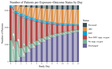
Figure 1: Alluvial plot showing the movement of patients between exposure and outcome statuses across study days. The exposure contains three levels: no supplemental oxygen, supplemental oxygen not including IMV, and IMV. The outcome of interest is AKI, and death is a competing risk. Patients who are discharged are right-censored.

4.3 Results

We estimate the effect of the LMTP with the SDR estimator (on account of its enhanced robustness relative to TMLE), using a version of the lmtp R package (Williams et al., 2022) modified to support the competing risks setting. The nuisance functions $\mathsf{r}_{t}$ and $\mathsf{m}_{t}$ are estimated using the Super Learner ensemble modeling algorithm (van der Laan et al., 2007) via the sl3 R package (Coyle et al., 2022). The candidate library considered by the Super Learner included a total of 32 learning algorithms, inclusive of hyperparameter variations. The algorithms included multivariate adaptive regression splines (MARS; Friedman et al., 1991); random forests (Breiman, 2001; Wright & Ziegler, 2017); extreme gradient boosted trees (Friedman, 2001; Chen & Guestrin, 2016); lasso, ridge, and elastic net (with equal weights, i.e., $\alpha=0.5$) regularized regression (Friedman et al., 2022); main terms generalized linear models (McCullagh & Nelder, 1989; Enea, 2009); generalized linear models with Bayesian priors on parameter estimates (Gelman & Hill, 2006); and an unadjusted outcome mean. The estimators of $\mathsf{r}_{t}$ and $\mathsf{m}_{t}$ were computed under a Markov assumption with lag $r=2$ to reflect the collection of laboratory results at minimum 48-hour intervals. Figure 2 displays the SDR-based cumulative event curve estimates for each treatment condition (panel A) after the correction for monotonicity proposed by Westling et al. (2020), and the incidence difference between the two (panel B), together with 95% simultaneous confidence bands.

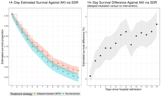
Figure 2: Panel A: Estimated AKI incidence across the arms defined by the two treatment strategies, 1-day delay-of-intubation and no intervention. Panel B: The time-specific difference between the two treatment conditions. In both panels, 95% simultaneous confidence bands cover the sets of point estimates.

Examination of Figure 2 panel A reveals a slight but increasingly widening gap (across days) between the SDR-based incidence estimates for each arm. In agreement with this, inspection of panel B of Figure 2 makes apparent the protective effect of the delay-in-intubation policy against AKI. The estimates of the incidence difference are consistently negative and decrease steadily in time; moreover, the simultaneous confidence bands do not overlap with the null value of zero except for on the first day. Hypothesis testing of the incidence difference yields adjusted p-values $<0.001$ for all days after the first, indicating a statistically significant protective effect of the LMTP; the Bonferroni correction was used to adjust for testing multiplicity. Based on these estimates, the delay-in-intubation policy would be expected to result in a decrease in 14-day AKI rates by approximately 3.5% (simultaneous 95% CI: [2.7%, 4.3%]) relative to no intervention.

5 Discussion

Modified treatment policies represent a recent but powerful advance in modern causal inference. These intervention regimes have a variety of applications, including (i) practical solutions to violations of the positivity assumption; (ii) definition and estimation of the effects of continuous, time-valued, and multivariate exposures; and (iii) definition of effects that depend on the natural value of treatment. Here, we have advanced the LMTP methodology, extending it to the case of survival outcomes with competing events. We have presented identification assumptions for the causal parameters, as well as a sequentially doubly robust and efficient estimation algorithm capable of leveraging the many data-adaptive regression procedures available for nuisance parameter estimation. We ensure that the estimates of the survival function remain within the parameter space (antitonic and bounded in the closed unit interval) by leveraging the monotonic projection framework of Westling & Carone (2020) and Westling et al. (2020). We have illustrated the scientific utility of our approach through application to the study of negative side effects of invasive mechanical ventilation on acute kidney injury in patients hospitalized with COVID-19, for which death by other causes serves as a competing event.

Our Proposition 2 shows that doubly robust estimation is possible for any intervention that is defined in terms of an LMTP satisfying the stated conditions. Namely, any randomized intervention defined by a known function $\mathbbm{d}(a_{t},h_{t},\varepsilon_{t})$ through either an LMTP or a general stochastic intervention accommodates doubly robust estimation, provided that: (1) either (i) $A_{t}$ is a discrete random variable for all $t$, or (ii) $A_{t}$ is a continuous random variable and the modified treatment policy $\mathbbm{d}$ satisfies Assumption 1, and (2) the randomizer $\varepsilon_{t}$ is drawn independently across units and independently of $U$, and its distribution does not depend on $\mathsf{P}$. Notably, this rich class contains all interventions considered by Theorem 2 of Wen et al. (2021).

Conflict of Interest

The authors declare that they have no conflict of interest.

References

- Andersen & Gill (1982) Andersen, P. & Gill, R. D. (1982). Cox’s regression model for counting processes: a large sample study. Annals of Statistics , 1100–1120.
- Bang & Robins (2005) Bang, H. & Robins, J. M. (2005). Doubly robust estimation in missing data and causal inference models. Biometrics 61, 962–973.
- Bavishi et al. (2021) Bavishi, A. A., Mylvaganam, R. J., Agarwal, R., Avery, R. J. & Cuttica, M. J. (2021). Timing of intubation in coronavirus disease 2019: A study of ventilator mechanics, imaging, findings, and outcomes. Critical Care Explorations 3.
- Benkeser et al. (2018) Benkeser, D., Carone, M. & Gilbert, P. B. (2018). Improved estimation of the cumulative incidence of rare outcomes. Statistics in Medicine 37, 280–293.
- Bickel (1982) Bickel, P. J. (1982). On adaptive estimation. Annals of Statistics , 647–671.
- Bickel et al. (1997) Bickel, P. J., Klaassen, C. A., Ritov, Y. & Wellner, J. A. (1997). Efficient and Adaptive Estimation for Semiparametric Models. Springer-Verlag.
- Breiman (1996) Breiman, L. (1996). Stacked regressions. Machine Learning 24, 49–64.
- Breiman (2001) Breiman, L. (2001). Random forests. Machine learning 45, 5–32.
- Buckley & James (1979) Buckley, J. & James, I. (1979). Linear regression with censored data. Biometrika 66, 429–436.
- Cain et al. (2010) Cain, L. E., Robins, J. M., Lanoy, E., Logan, R., Costagliola, D. & Hernán, M. A. (2010). When to start treatment? a systematic approach to the comparison of dynamic regimes using observational data. International Journal of Biostatistics 6.
- Chen & Guestrin (2016) Chen, T. & Guestrin, C. (2016). Xgboost: A scalable tree boosting system. In Proceedings of the 22nd ACM SIGKDD International Conference on Knowledge Discovery and Data Mining. ACM.
- Chernozhukov et al. (2017) Chernozhukov, V., Chetverikov, D., Demirer, M., Duflo, E., Hansen, C. & Newey, W. (2017). Double/debiased/neyman machine learning of treatment effects. American Economic Review 107, 261–65.
- Chernozhukov et al. (2018) Chernozhukov, V., Chetverikov, D., Demirer, M., Duflo, E., Hansen, C., Newey, W. & Robins, J. (2018). Double/debiased machine learning for treatment and structural parameters. The Econometrics Journal 21, C1–C68.
- Cox (1972) Cox, D. R. (1972). Regression models and life-tables. Journal of the Royal Statistical Society: Series B (Statistical Methodology) 34, 187–202.
- Coyle et al. (2022) Coyle, J. R., Hejazi, N. S., Malenica, I., Phillips, R. V. & Sofrygin, O. (2022). sl3: Modern pipelines for machine learning and Super Learning. R package version 1.4.4.
- Díaz & Hejazi (2020) Díaz, I. & Hejazi, N. S. (2020). Causal mediation analysis for stochastic interventions. Journal of the Royal Statistical Society: Series B (Statistical Methodology) 82, 661–683.
- Díaz et al. (2020) Díaz, I., Hejazi, N. S., Rudolph, K. E. & van der Laan, M. J. (2020). Non-parametric efficient causal mediation with intermediate confounders. Biometrika 108, 627–641.
- Díaz & van der Laan (2012) Díaz, I. & van der Laan, M. J. (2012). Population intervention causal effects based on stochastic interventions. Biometrics 68, 541–549.
- Díaz & van der Laan (2018) Díaz, I. & van der Laan, M. J. (2018). Stochastic treatment regimes. In Targeted Learning in Data Science: Causal Inference for Complex Longitudinal Studies. Springer, pp. 219–232.
- Díaz et al. (2021) Díaz, I., Williams, N., Hoffman, K. L. & Schenck, E. J. (2021). Nonparametric causal effects based on longitudinal modified treatment policies. Journal of the American Statistical Association , 1–16.
- Durdevic et al. (2020) Durdevic, M., Durdevic, D., Riera, M. B., Nimkar, A., Stan, A. C., Hasan, A., Naaraayan, A. & Jesmajian, S. (2020). Progressive renal failure in patients with covid-19 after initiating mechanical ventilation: A case series. Chest 158, A2629.
- Enea (2009) Enea, M. (2009). Fitting linear models and generalized linear models with large data sets in R. In Statistical Methods for the Analysis of Large Datasets. pp. 411–414.
- Fine & Gray (1999) Fine, J. P. & Gray, R. J. (1999). A proportional hazards model for the subdistribution of a competing risk. Journal of the American Statistical Association 94, 496–509.
- Friedman et al. (2022) Friedman, J., Hastie, T., Tibshirani, R., Narasimhan, B., Tay, K., Simon, N. & Yang, J. (2022). glmnet: Lasso and elastic-net regularized generalized linear models. R package version 4.1-3.
- Friedman (2001) Friedman, J. H. (2001). Greedy function approximation: a gradient boosting machine. Annals of Statistics , 1189–1232.
- Friedman et al. (1991) Friedman, J. H. et al. (1991). Multivariate adaptive regression splines. Annals of Statistics 19, 1–67.
- Gelman & Hill (2006) Gelman, A. & Hill, J. (2006). Data Analysis Using Regression and Multilevel/Hierarchical Models. Cambridge university press.
- Gibson et al. (2019) Gibson, E. A., Nunez, Y., Abuawad, A., Zota, A. R., Renzetti, S., Devick, K. L., Gennings, C., Goldsmith, J., Coull, B. A. & Kioumourtzoglou, M.-A. (2019). An overview of methods to address distinct research questions on environmental mixtures: an application to persistent organic pollutants and leukocyte telomere length. Environmental Health 18, 1–16.
- Goyal et al. (2020) Goyal, P., Choi, J. J., Pinheiro, L. C., Schenck, E. J., Chen, R., Jabri, A., Satlin, M. J., Campion Jr, T. R., Nahid, M., Ringel, J. B. et al. (2020). Clinical characteristics of covid-19 in new york city. New England Journal of Medicine 382, 2372–2374.
- Haneuse & Rotnitzky (2013) Haneuse, S. & Rotnitzky, A. (2013). Estimation of the effect of interventions that modify the received treatment. Statistics in Medicine .
- Hasan et al. (2020) Hasan, S. S., Capstick, T., Ahmed, R., Kow, C. S., Mazhar, F., Merchant, H. A. & Zaidi, S. T. R. (2020). Mortality in covid-19 patients with acute respiratory distress syndrome and corticosteroids use: a systematic review and meta-analysis. Expert Review of Respiratory Medicine 14, 1149–1163.
- Hejazi et al. (2022) Hejazi, N. S., Rudolph, K. E., van der Laan, M. J. & Díaz, I. (2022). Nonparametric causal mediation analysis for stochastic interventional (in) direct effects. Biostatistics in press.
- Hejazi et al. (2020) Hejazi, N. S., van der Laan, M. J., Janes, H. E., Gilbert, P. B. & Benkeser, D. C. (2020). Efficient nonparametric inference on the effects of stochastic interventions under two-phase sampling, with applications to vaccine efficacy trials. Biometrics 77, 1241–1253.
- Husain-Syed et al. (2016) Husain-Syed, F., Slutsky, A. S. & Ronco, C. (2016). Lung–kidney cross-talk in the critically ill patient. American Journal of Respiratory and Critical Care Medicine 194, 402–414.
- Joannidis et al. (2020) Joannidis, M., Forni, L. G., Klein, S. J., Honore, P. M., Kashani, K., Ostermann, M., Prowle, J., Bagshaw, S. M., Cantaluppi, V., Darmon, M. et al. (2020). Lung–kidney interactions in critically ill patients: consensus report of the acute disease quality initiative (adqi) 21 workgroup. Intensive Care Medicine 46, 654–672.
- Kennedy (2019) Kennedy, E. H. (2019). Nonparametric causal effects based on incremental propensity score interventions. Journal of the American Statistical Association 114, 645–656.
- Kes & Jukić (2010) Kes, P. & Jukić, N. B. (2010). Acute kidney injury in the intensive care unit. Bosnian Journal of Basic Medical Sciences 10, S8.
- Klaassen (1987) Klaassen, C. A. (1987). Consistent estimation of the influence function of locally asymptotically linear estimators. Annals of Statistics 15, 1548–1562.
- Luedtke et al. (2017) Luedtke, A. R., Sofrygin, O., van der Laan, M. J. & Carone, M. (2017). Sequential double robustness in right-censored longitudinal models. arXiv preprint arXiv:1705.02459 .
- McCullagh & Nelder (1989) McCullagh, P. & Nelder, J. A. (1989). Generalized Linear Models. CRC Press.
- Papoutsi et al. (2021) Papoutsi, E., Giannakoulis, V. G., Xourgia, E., Routsi, C., Kotanidou, A. & Siempos, I. I. (2021). Effect of timing of intubation on clinical outcomes of critically ill patients with covid-19: a systematic review and meta-analysis of non-randomized cohort studies. Critical Care 25, 1–9.
- Pearl (2000) Pearl, J. (2000). Causality: Models, Reasoning, and Inference. Cambridge University Press.
- Perkins et al. (2020) Perkins, G. D., Couper, K., Connolly, B., Baillie, J. K., Bradley, J. M., Dark, P., De Soyza, A., Gorman, E., Gray, A., Hamilton, L. et al. (2020). Recovery-respiratory support: Respiratory strategies for patients with suspected or proven covid-19 respiratory failure; continuous positive airway pressure, high-flow nasal oxygen, and standard care: A structured summary of a study protocol for a randomised controlled trial. Trials 21, 1–3.
- Prentice et al. (1978) Prentice, R. L., Kalbfleisch, J. D., Peterson Jr, A. V., Flournoy, N., Farewell, V. T. & Breslow, N. E. (1978). The analysis of failure times in the presence of competing risks. Biometrics , 541–554.
- Richardson & Robins (2013) Richardson, T. S. & Robins, J. M. (2013). Single world intervention graphs (SWIGs): A unification of the counterfactual and graphical approaches to causality. Center for the Statistics and the Social Sciences, University of Washington Series. Working Paper 128, 2013.
- Robins et al. (2009) Robins, J., Li, L., Tchetgen Tchetgen, E. & van der Vaart, A. W. (2009). Quadratic semiparametric von Mises calculus. Metrika 69, 227–247.
- Robins (2000) Robins, J. M. (2000). Robust estimation in sequentially ignorable missing data and causal inference models. In Proceedings of the American Statistical Association.
- Robins et al. (2004) Robins, J. M., Hernán, M. A. & Siebert, U. (2004). Effects of multiple interventions. Comparative quantification of health risks: global and regional burden of disease attributable to selected major risk factors 1, 2191–2230.
- Robins et al. (1994) Robins, J. M., Rotnitzky, A. & Zhao, L. (1994). Estimation of regression coefficients when some regressors are not always observed. Journal of the American Statistical Association 89, 846–866.
- Rotnitzky et al. (2017) Rotnitzky, A., Robins, J. & Babino, L. (2017). On the multiply robust estimation of the mean of the g-functional. arXiv preprint arXiv:1705.08582 .
- Rubin & van der Laan (2007) Rubin, D. & van der Laan, M. J. (2007). A doubly robust censoring unbiased transformation. International Journal of Biostatistics 3.
- Rudolph et al. (2021) Rudolph, K. E., Gimbrone, C., Matthay, E. C., Diaz, I., Davis, C. S., Pamplin II, J. R., Keyes, K. & Cerda, M. (2021). When effects cannot be estimated: redefining estimands to understand the effects of naloxone access laws. arXiv preprint arXiv:2105.02757 .
- Rytgaard & van der Laan (2021) Rytgaard, H. C. & van der Laan, M. J. (2021). One-step tmle for targeting cause-specific absolute risks and survival curves. arXiv preprint arXiv:2107.01537 .
- Schenck et al. (2021) Schenck, E. J., Hoffman, K. L., Cusick, M., Kabariti, J., Sholle, E. T. & Campion Jr, T. R. (2021). Critical care database for advanced research (cedar): An automated method to support intensive care units with electronic health record data. Journal of Biomedical Informatics 118, 103789.
- Stock (1989) Stock, J. H. (1989). Nonparametric policy analysis. Journal of the American Statistical Association 84, 567–575.
- Thomson & Calligaro (2021) Thomson, D. A. & Calligaro, G. L. (2021). Timing of intubation in COVID-19: Not just location, location, location? Critical Care 25, 1–2.
- Tobin (2006) Tobin, M. J. (2006). Principles and practice of mechanical ventilation.
- Tobin (2020) Tobin, M. J. (2020). Basing respiratory management of COVID-19 on physiological principles. American Journal of Respiratory and Critical Care Medicine 201, 1319–1320. PMID: 32281885.
- Tobin et al. (2020) Tobin, M. J., Laghi, F. & Jubran, A. (2020). Caution about early intubation and mechanical ventilation in covid-19. Annals of Intensive Care 10, 1–3.
- van Buuren & Groothuis-Oudshoorn (2011) van Buuren, S. & Groothuis-Oudshoorn, K. (2011). mice: Multivariate imputation by chained equations in R. Journal of Statistical Software 45, 1–67.
- van der Laan et al. (2006) van der Laan, M. J., Dudoit, S. & van der Vaart, A. W. (2006). The cross-validated adaptive epsilon-net estimator. Statistics & Decisions 24, 373–395.
- van der Laan et al. (2005) van der Laan, M. J., Petersen, M. L. & Joffe, M. M. (2005). History-adjusted marginal structural models and statically-optimal dynamic treatment regimens. International Journal of Biostatistics 1.
- van der Laan et al. (2007) van der Laan, M. J., Polley, E. C. & Hubbard, A. E. (2007). Super learner. Statistical Applications in Genetics & Molecular Biology 6, Article 25.
- van der Laan & Robins (2003) van der Laan, M. J. & Robins, J. M. (2003). Unified Methods for Censored Longitudinal Data and Causality. Springer, New York.
- van der Laan & Rose (2011) van der Laan, M. J. & Rose, S. (2011). Targeted Learning: Causal Inference for Observational and Experimental Data. New York: Springer.
- van der Laan & Rose (2018) van der Laan, M. J. & Rose, S. (2018). Targeted Learning in Data Science: Causal Inference for Complex longitudinal Studies. New York: Springer.
- van der Laan & Rubin (2006) van der Laan, M. J. & Rubin, D. (2006). Targeted maximum likelihood learning. International Journal of Biostatistics 2.
- van der Vaart (1998) van der Vaart, A. W. (1998). Asymptotic Statistics. Cambridge University Press.
- VanderWeele et al. (2014) VanderWeele, T. J., Vansteelandt, S. & Robins, J. M. (2014). Effect decomposition in the presence of an exposure-induced mediator-outcome confounder. Epidemiology 25, 300.
- von Mises (1947) von Mises, R. (1947). On the asymptotic distribution of differentiable statistical functions. The Annals of Mathematical Statistics 18, 309–348.
- Wen et al. (2021) Wen, L., Marcus, J. & Young, J. (2021). Intervention treatment distributions that depend on the observed treatment process and model double robustness in causal survival analysis. arXiv preprint arXiv:2112.00807 .
- Westling & Carone (2020) Westling, T. & Carone, M. (2020). A unified study of nonparametric inference for monotone functions. Annals of Statistics 48, 1001.
- Westling et al. (2020) Westling, T., van der Laan, M. J. & Carone, M. (2020). Correcting an estimator of a multivariate monotone function with isotonic regression. Electronic Journal of Statistics 14, 3032–3069.
- Williams et al. (2022) Williams, N. T., Hoffman, K. L. & Díaz, I. (2022). lmtp: Non-parametric causal effects of feasible interventions based on modified treatment policies. R package version 1.0.1.
- Wolpert (1992) Wolpert, D. H. (1992). Stacked generalization. Neural Networks 5, 241–259.
- Wright & Ziegler (2017) Wright, M. N. & Ziegler, A. (2017). ranger: A fast implementation of random forests for high dimensional data in C++ and R. Journal of Statistical Software 77.
- Young et al. (2014) Young, J. G., Hernán, M. A. & Robins, J. M. (2014). Identification, estimation and approximation of risk under interventions that depend on the natural value of treatment using observational data. Epidemiologic Methods 3, 1–19.
- Young et al. (2020) Young, J. G., Stensrud, M. J., Tchetgen Tchetgen, E. J. & Hernán, M. A. (2020). A causal framework for classical statistical estimands in failure-time settings with competing events. Statistics in Medicine 39, 1199–1236.
- Zheng & van der Laan (2011) Zheng, W. & van der Laan, M. J. (2011). Cross-validated targeted minimum-loss-based estimation. In Targeted Learning: Causal Inference for Observational and Experimental Data. Springer, pp. 459–474.