Navigating Neural Space: Revisiting Concept Activation Vectors
to Overcome Directional Divergence

Abstract

With a growing interest in understanding neural network prediction strategies, Concept Activation Vectors (CAVs) have emerged as a popular tool for modeling human-understandable concepts in the latent space. Commonly, CAVs are computed by leveraging linear classifiers optimizing the separability of latent representations of samples with and without a given concept. However, in this paper we show that such a separability-oriented computation leads to solutions, which may diverge from the actual goal of precisely modeling the concept direction. This discrepancy can be attributed to the significant influence of distractor directions, i.e., signals unrelated to the concept, which are picked up by filters (i.e., weights) of linear models to optimize class-separability. To address this, we introduce pattern-based CAVs, solely focussing on concept signals, thereby providing more accurate concept directions. We evaluate various CAV methods in terms of their alignment with the true concept direction and their impact on CAV applications, including concept sensitivity testing and model correction for shortcut behavior caused by data artifacts. We demonstrate the benefits of pattern-based CAVs using the Pediatric Bone Age, ISIC2019, and FunnyBirds datasets with VGG, ResNet, and EfficientNet model architectures.

1 Introduction

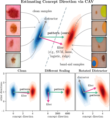
Figure 1: CAVs obtained from filters, i.e. weight vectors from linear classifiers, are optimized for class separability, but fail at precisely estimating concept signal directions. Top: Different CAV computation strategies are employed to estimate the “band-aid” concept, a confounding artifact present in the ISIC2019 dataset. Bottom: Weaknesses of filter-based CAVs are apparent for simple transformations in a 2D toy experiment, where we scale concept features (x-axis) differently than other (e.g., distracting) features (middle) or rotate distracting directions (right). Only the pattern-based CAV precisely estimates the concept signal direction, while the filter-based CAV diverges to optimize class separability. Animated visualizations for these and additional 2D experiments can be found here: http://tinyurl.com/ymywcwmo.

In recent years, eXplainable Artificial Intelligence (XAI) has gained increased interest, as Deep Neural Networks (DNNs) are ubiquitous in high-stake decision processes, such as medicine [7], finance [34], and criminal justice [43, 38], with black-box predictions being unacceptable. Whereas local explainability methods compute the relevance of input features for individual predictions, global XAI approaches aim at identifying global prediction strategies employed by the model, often to be represented as human-understandable concepts. Backed by recent research, suggesting that DNNs encode concepts as superpositions in latent space [2, 16, 28, 41], Concept Activation Vectors (CAVs), originally introduced for concept sensitivity testing [24], model concepts in DNNs by finding directions pointing from samples without the concept to samples with the concept. Commonly, the direction is estimated by taking the weight vector of a linear classifier (e.g., a linear Support Vector Machine (SVM)), representing the normal to the decision hyperplane separating the two sample sets. However, while linear classifiers optimize the separability of two classes, they might fail at precisely identifying the signal direction encoding the concept. This can be attributed to the significant influence of distractor (i.e., non-signal) directions contained in the data, which are picked up by filters (i.e., weights) of linear models to optimize class-separability [20]. This decomposition of filters into signal and distractor patterns has also been addressed in the context of local explainability methods [25]. We follow their approach and introduce pattern-based CAVs, disregarding distractors and thereby precisely estimating the concept signal direction (see Fig. 1).

Despite directional divergence from the true concept signal, CAVs have been employed for a plethora of tasks in recent years, such as concept sensitivity testing [24], model correction for shortcut removal  [4, 30, 15], knowledge discovery by investigation of internal model states [27], and training of post-hoc concept bottleneck models [42]. Many of these applications can be improved by more precise concept directions, as provided by pattern-CAVs, instead of optimized class-separability, as provided by filters. To demonstrate the superiority of pattern-CAVs in these scenarios, we run controlled and non-controlled experiments using the Pediatric Bone Age, ISIC2019, and FunnyBirds datasets with VGG16, ResNet18 and EfficientNet-B0 model architectures. Our main contributions include the following:

1. We introduce pattern-CAVs, more precisely estimating the concept signal direction and being less influenced by distractors.

2. We measure the alignment of CAVs with the true concept direction in controlled settings, confirming that pattern-CAVs align with the true concept direction, while the widely used filter-CAVs diverge.

3. We measure the impact of directional shifts in popular CAV applications, including Testing with CAV (TCAV) and model correction with Class Artifact Compensation (ClArC) in controlled and real-world experiments, demonstrating benefits of pattern-CAV in both cases.

2 Related Work

A variety of approaches have emerged to identify human-understandable concepts in DNNs. Some works consider single neurons as concepts [29, 1], while others focus on identifying interesting subspaces [40] or linear directions [28]. We follow the latter approach, where concepts are encoded as linear combinations, also known as superpositions, of neurons [16]. These directions can be identified through unsupervised matrix factorization [17] or by fitting CAVs, i.e., vectors pointing from samples without to samples with the concept. Automated concept discovery approaches can further streamline this process [18]. CAVs are leveraged by various methods to model concepts in latent space. For instance, TCAV measures a model’s sensitivity towards specific concepts. ClArC aims to unlearn model shortcuts, i.e., prediction strategies based on unintended correlations between target labels and data artifacts, represented by CAVs. Post-hoc concept bottleneck models project latent representations into a space spanned by CAVs to obtain an interpretable latent representation. Beyond these applications, CAVs have been employed to understand the strategies learned by AlphaZero in playing chess [27] and to identify meaningful directions for manipulation (e.g. no-smile $\rightarrow$ smile) in diffusion autoencoders [32]. Related works aim to enhance CAV robustness by alleviating the linear separability assumption [8, 31], for example by representing concepts as regions [13]. In contrast, our approach adheres to the linear separability assumption but improves the precision of the modeled direction.

3 Estimating Signal of Concept Direction

We view a DNN as a function $f:\mathcal{X}\rightarrow\mathcal{Y}$, mapping input samples $\mathbf{x}\in\mathcal{X}$ to target labels $y\in\mathcal{Y}$. Without loss of generality, we assume that at any layer $l$ with $m$ neurons, $f$ can be split into a feature extractor $\mathbf{a}:\mathcal{X}\rightarrow\mathbb{R}^{m}$, computing latent activations at layer $l$, and a model head $\tilde{f}:\mathbb{R}^{m}\rightarrow\mathcal{Y}$, mapping latent activations to target labels. We further assume binary concept labels $t\in\{+1,-1\}$. CAVs are intended to point from latent activations of samples without concept $\mathcal{A}^{-}=\{\mathbf{a}(\mathbf{x}_{i})\in\mathbb{R}^{m}\mid t_{i}=-1\}$ to activations of samples with concept $\mathcal{A}^{+}=\{\mathbf{a}(\mathbf{x}_{i})\in\mathbb{R}^{m}\mid t_{i}=+1\}$. The optimal choice of layer $l$ depends on the type of concept, as simple concepts (e.g., color and edges) are learned on earlier layers, while more abstract concepts (e.g., the band-aid concept) are learned closer to the model output [29, 33, 6].

3.1 Filter-based CAV Computation

Traditionally, a CAV $\mathbf{h}$ is identified as the weight vector $\mathbf{w}\in\mathbb{R}^{m}$ from a linear classifier, that describes a hyperplane separating latent activations of samples with the concept $\mathcal{A}^{+}$ from activations of samples without the concept $\mathcal{A}^{-}$. Most commonly (e.g., [24, 3, 42]), linear SVMs are employed, minimizing the hinge loss with L2 regularization [12]. Other options include Lasso [37], Logistic, or Ridge [23] regression.

Concretely, the classification task is usually described as a linear regression problem. With concept labels $t$ as dependent variable and latent activations $\mathbf{a}(\mathbf{x})\in\mathbb{R}^{m}$ as regressors, we assume a linear model $f_{\text{linear}}(\mathbf{x})=\mathbf{h}^{\top}\mathbf{a}(\mathbf{x})+b$ with weight vector (or filter) ${\mathbf{h}\in\mathbb{R}^{m}}$ and bias $b\in\mathbb{R}$. Using ridge regression as an example, the optimization task to find a filter-CAV $\mathbf{h}^{\text{filt}}$ is then given by

$$\mathbf{h}^{\text{filt}}:\min_{\mathbf{h},\mathbf{b}}\left\|\mathbf{t}-A\mathbf{h}-\mathbf{b}\right\|_{2}+\lambda\left\|\mathbf{h}\right\|_{2}\\$$ (1)

with $\mathbf{t}\in\mathbb{R}^{n}$ representing a vector with concept label $t_{i}$ as the $i^{\text{th}}$ element, $\mathbf{b}\in\mathbb{R}^{n}$ as an $n$-wise repetition of $b$, and $A\in\mathbb{R}^{n\times m}$ summarizing latent activations for all $n$ samples in $\mathcal{X}$ in matrix form. The optimization objectives differ by the type of linear model (see Appendix A.1).

However, research from the neuroimaging realm suggests that filters from linear classifiers not only model the signal separating the two classes but also capture a distractor component. This component can arise from noise, but also from unrelated features in the data, which are not directly related to the signal  [20]. In the context of CAVs, any information unrelated to concept label $t$ is considered a distractor. The filters are optimized to weigh all features to achieve optimal separability w.r.t. $t$. However, this optimization does not disentangle concept signals from distractor signals. As a result, distractor pattern present in the training data influence the direction of filter-CAVs.

3.2 Pattern-based CAV

We introduce a pattern-based CAV, which is based on the assumption that, given latent activations $\mathcal{A}$, there is a linear dependency between signal $s=p_{s}t$ and concept label $t$. The signal pattern $p_{s}$ can be obtained optimizing the following task  [20]:

$$\mathbf{h}^{\text{pat}}:\min_{\mathbf{h},\mathbf{b}}\left\|A-\mathbf{t}\mathbf{h}^{\top}-\mathbf{b}\right\|_{2}~{}.\\$$ (2)

In contrast to Eq. (1) which aims to find an $\mathbf{h}$ maximizing the class-separability, Eq. (2) finds a pattern best explaining $\mathcal{A}$ w.r.t. concept label $t$. This can be solved as a simple linear regression task for each feature dimension, leading to

$$\mathbf{h}^{\text{pat}}=\frac{\text{cov}[\mathcal{A},t]}{\sigma_{t}^{2}}\sim\sum_{\mathbf{x},t\in\mathcal{X}}(\mathbf{a}(\mathbf{x})-\bar{\mathcal{A}})(t-\bar{t})$$ (3)

with mean latent activation $\bar{\mathcal{A}}$ and mean concept label $\bar{t}$. Contrary to filter-CAVs, the resulting pattern-CAV is invariant under feature scaling and more robust to noise, as further outlined in Appendix A.2. Given binary concept labels, Eq. (3) simplifies to the difference of cluster means, as shown in Appendix A.3. Note, that the computation of pattern in regression manner as described in Eq. (3) allows to further incorporate prior knowledge, e.g., sparseness constraints [20].

3.3 2D Toy Experiments

We demonstrate the difference between filter- and pattern-CAVs in a toy experiment inspired by [25]. We generate $n$ simulated activations $A_{i}\in\mathbb{R}^{2}$ split equally between the concept labels $t_{i}\in\{+1,-1\}$ in the following manner: Each activation $A_{i}=s_{i}+D_{i}$ may be decomposed into a deterministic signal part $s_{i}$ and a random (non-signal-, noise-) distractor part $D_{i}$. The signal part $s_{i}=p_{s}\mathbbm{1}(t_{i}=+1)$ with signal pattern $p_{s}=(1~{}~{}0)^{\top}$ (x-axis) is equal to the signal pattern vector $p_{s}$ if the datapoint is in the concept class, and 0 otherwise. The distractor part $D_{i}$ is modeled by identically distributed independent two-dimensional Gaussians of mean 0, variance $\sigma^{2}$ in each dimension and no correlation between dimensions. We experiment with two distractor patterns in Figure 1 (bottom):

Scaling (Fig. 1, bottom, middle): We multiply values on the x-axis with scaling factor $\lambda=10^{3}$, such that the signal pattern $p_{s}$ is scaled proportionally and therefore signal features are on a larger scale than distractor features. The filter-CAV diverges from the true concept direction $p_{s}$, as the entry of the weight vector in direction of the signal scales anti-proportionally to the scaling factor in logistic regression (see Appendix A.5 for the mathematical derivation). This can be addressed via feature normalization, which is commonly disregarded in CAV training.

Noise Rotation (Fig. 1, bottom, right): We add another distractor term $D^{rot}_{i}=r_{\tau}\varepsilon_{i}$ with $\varepsilon_{i}\stackrel{{\scriptstyle i.i.d.}}{{\sim}}\mathcal{N}(0,1)$, which is oriented parallel to the vector $r_{\tau}=(\sin\tau~{}~{}\cos\tau)^{\top}$. This rotates the distractor direction based on $\tau$. Only the pattern-CAV $\mathbf{h}^{\text{pat}}$ obtained via Eq. (3) precisely identifies the concept direction $p_{s}$, while the filter-CAV prefers diverging directions which increase the angle to $r_{\tau}$, thus minimizing the variance of the datapoints in direction of the weight vector (see Appendix A.6 for the mathematical derivation).

Moreover, filter-based CAVs face further challenges, including sensitivity to regularization strength and random seeds, particularly in low data scenarios. This is demonstrated in additional visualizations in Appendix A.4.

4 Experiments

After describing our experimental setup (Section 4.1), we address the following research questions:

1. How precise do CAVs represent true concept directions (Section 4.2)?

2. What is the impact of CAVs on applications, including concept sensitivity testing with TCAV (Section 4.3.1) and CAV-based model correction (Section 4.3.2)?

4.1 Experiment Details

We conduct experiments with three controlled and one real-word datasets. For the former, we insert artificial concepts into ISIC2019 [9, 39, 10], a dermatologic dataset for skin cancer detection with images of benign and malignant lesions, and a Pediatric Bone Age dataset [19], with the task to predict bone age based on hand radiographs. Specifically, we insert timestamps as a text layover into $1$% of samples of class “Melanoma” of ISIC2019, encouraging the model to learn the timestamps as a shortcut. For the Bone Age dataset, we insert an unlocalizable concept by increasing the brightness (i.e., increase pixel values) of $20$% of samples of only one class. We implemented bone age prediction as a classification task, with target ages binned into five equal-sized groups. Lastly, we use FunnyBirds [22], a synthetic dataset with part-level annotations, to synthesize a dataset with 10 classes of birds, where each category is defined by exactly one part (e.g., wings, beak). Other parts are chosen randomly per sample, forcing the model to use the class-defining part (i.e., concept) as the only valid feature. Detailed class definitions and examples for synthesized images are provided in Appendix B.1. Further, we consider real data artifacts present in ISIC2019, including “band-aid”, “ruler”, and “skin marker”. We train VGG16 [35], ResNet18 [21], and EfficientNet-B0 [36] models for all datasets, with training details given in Appendix B.2.

4.2 Preciseness of Concept Representation

To assess how precise CAVs represent true concept directions both qualitatively and quantitatively, we (1) visualize the key neurons associated with the CAV, and (2) quantify the alignment between CAVs and the ground truth direction.

How clean are CAVs qualitatively?

We investigate the focus of CAV $\mathbf{h}$ fitted on layer $l$ by employing feature visualization to neurons corresponding to the largest absolute, hence most impactful, values in $\mathbf{h}$. Specifically, we use RelMax [1] to retrieve input samples maximizing the relevance, computed by feature attribution methods, for the neurons with the largest absolute values in $\mathbf{h}$. We further use receptive field information to zoom into the most relevant region and mask out irrelevant information. Results for filter- and pattern-based CAVs for the timestamp artifact in ISIC2019 are shown in Fig. 2. Whereas the pattern-CAV leverages neurons focusing on the desired concept, i.e., the timestamp, the filter-CAV is distracted by other features. Additional neuron visualizations for different filter- and pattern-CAVs are shown in Appendix C.2.

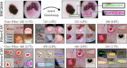
Figure 2: Example for timestamp artifact inserted into ISIC2019 samples (top) and RelMax visualization for neurons corresponding to the largest absolute values in filter- (middle) and pattern-CAVs (bottom), along with the Conv filter ID and the fraction of all (absolute) CAV values. While the filter-CAV picks up noisy neurons, the pattern-CAV uses neurons related to the relevant concept.

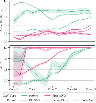
Figure 3: Comparison of cosine similarity between CAVs and true concept direction (top) and concept separability as AUC (bottom), using filter- (SVM) and pattern-CAV for all Conv layers of VGG16 trained on ISIC2019, Bone Age, and FunnyBirds datasets. While expectedly filter-CAVs have superior class-separability, pattern-CAVs have a better alignment with the true concept direction.

CAV Alignment with True Concept Direction

Using our controlled datasets, we generate pairs of samples with and without the concept ($\mathbf{x^{+}}$ and $\mathbf{x^{-}}$, respectively). To quantify the alignment between the CAV $\mathbf{h}$ and $\mathbf{h}^{\text{gt}}$ for each sample, we use cosine similarity as the similarity function $\text{sim}(\mathbf{h},\mathbf{h}^{\text{gt}})$. We calculate the overall alignment $\bar{a}$ by averaging the alignment scores across all samples:

$$\bar{a}=\frac{1}{|\mathcal{X}|}\sum\text{sim}(\mathbf{h},\mathbf{h}^{\text{gt}}_{i})~{}\text{.}$$ (4)

Moreover, we measure the separability of samples w.r.t. concept label $t$ by computing the AUC of $\mathbf{h}^{\top}\mathbf{a}(\mathbf{x)}$. Fig. 3 presents the results, including standard errors, for both CAV alignment (top) and separability (bottom) across all 13 convolutional (Conv) layers in the VGG16 models for all three controlled datasets. We estimate standard errors of AUC scores using the Wilcoxon-Mann-Whitney statistic as an equivalence [11]. The alignment with $\mathbf{h}^{\text{gt}}$ is significantly higher for pattern-based CAVs across all layers for all datasets, confirming a more precise estimation of the true concept direction. As expected, filter-based CAVs exhibit higher concept separability.

We further investigate the sensitivity of CAVs to different feature pre-processing methods, specifically centering, max-scaling, and their combination. Results for CAVs fitted on the last Conv layer of VGG16 for ISIC2019 and Bone Age are shown in Fig. 4. While filter-CAVs exhibit better alignment with true concept directions when feature scaling is applied, which is often overlooked in practice, pattern-CAVs consistently outperform filter-CAVs regardless of feature pre-processing. This can be attributed to the fact that Pearson correlation is not affected by the scale and translation of variables. Another disadvantage of filter-CAVs is their dependence on hyperparameters, e.g., regularization strength. In contrast, pattern-CAVs do not require parameter tuning and are therefore more computationally efficient.

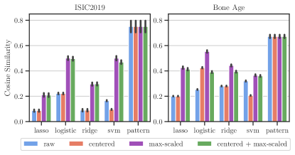
Figure 4: Cosine similarity between true concept direction $\mathbf{h}^{\text{gt}}$ and CAVs with different feature pre-processing methods fitted on the last Conv layer of VGG16 trained on ISIC2019 (left) and Bone Age (right). Compared to filter-CAVs, pattern-CAV has a higher alignment with $\mathbf{h}^{\text{gt}}$ and is invariant to feature pre-processing.

4.3 Impact of Directional Shifts on CAV Applications

We measure the impact of different CAVs on applications requiring precise concept directions, namely concept sensitivity testing with TCAV and model correction with ClArC.

4.3.1 Testing with CAV

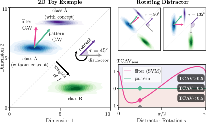
Figure 5: Left: 2D TCAV experiment with distractor rotated by $\tau=45^{\circ}$ with samples from class A (purple with concept, blue without concept) and class B (green). The model $f$ classifies between classes A and B. CAVs are fitted on samples with and without concept from class A. The pattern-CAV aligns with the concept direction, while the filter-CAV diverges to optimize class-separability. Right: $\text{TCAV}_{\text{sens}}$ for model $f$ plotted over distractor rotation $\tau$. Positive and negative values indicate a positive ($\text{TCAV}>0.5$) and negative ($\text{TCAV}<0.5$) influence of the concept direction and $0$ indicates insensitivity ($\text{TCAV}=0.5$).

TCAV [24] is a technique to assess the sensitivity of a DNNs’ prediction w.r.t. a given concept represented by CAV $\mathbf{h}$. Specifically, given the directional derivative $\boldsymbol{\nabla}_{\mathbf{a}}\tilde{f}(\mathbf{a}(\mathbf{x}))$, we measure the model’s sensitivity towards the concept for a sample $\mathbf{x}$ as

$$\text{TCAV}_{\text{sens}}(\mathbf{x})=\boldsymbol{\nabla}_{\mathbf{a}}\tilde{f}(\mathbf{a}(\mathbf{x}))\cdot\mathbf{h}~{}.$$ (5)

The TCAV score measures the fraction of the subset containing the concept $\mathcal{X}_{c}=\{\mathbf{x}_{i}\in\mathcal{X}\mid t_{i}=+1\}$ where the model exhibits positive sensitivity towards changes along the estimated concept direction $\mathbf{h}$ and is computed as

$$\text{TCAV}=\frac{|\{\mathbf{x}\in\mathcal{X}_{c}\mid\text{TCAV}_{\text{sens}}(\mathbf{x})>0\}|}{|\mathcal{X}_{c}|}\,.$$ (6)

Hence, in order to truthfully measure the model’s sensitivity, a precise estimated concept direction $\mathbf{h}$ is required. A TCAV score $\approx 0.5$ indicates minimal influence of the concept on the model’s decisions, while scores $>0.5$ and $<0.5$ indicate positive and negative impacts, respectively. We conduct experiments in 2D and with our controlled FunnyBirds dataset to demonstrate the effects of directional divergence.

TCAV in 2D Toy Experiment

Consider samples $x\in\mathbb{R}^{2}$ with class labels $y\in\{+1,-1\}$, referred to as class A and B, perfectly separable by a linear model $f$ with weights $\mathbf{w}=(1~{}-\!1)^{\top}$ and bias $\mathbf{b}=0$. We introduce a data artifact in class A where some samples contain concept $c$ with concept direction $\vec{c}=(1~{}~{}1)^{\top}$ perpendicular to $\mathbf{w}$. Thus, $f$ is insensitive to concept $c$, resulting in an expected TCAV score of $0.5$. Following the notation from Section 3.3, we rotate the distractor pattern $p_{d}$ with $\tau\in[0,\pi]$ relative to $\vec{c}$. CAVs are fitted to separate samples with and without $c$ from class A, using concept labels $t$ instead of class labels $y$. Results are shown in Fig. 5. For $\tau=\pi/4=45^{\circ}$(left), we observe that $\mathbf{h}^{\text{pat}}$ aligns with the concept direction $\vec{c}$, whereas $\mathbf{h}^{\text{filt}}$ diverges significantly from the true concept direction. Plotting the models sensitivity towards $c$, here measured as $\text{TCAV}_{\text{sens}}=\mathbf{w}^{\top}\mathbf{h}$, with $\mathbf{w}$ as the gradient of $f$ w.r.t. $\mathbf{x}$, over $\tau$ (right), we can see that $\mathbf{h}^{\text{pat}}$ consistently achieves $\text{TCAV}_{\text{sens}}=0$ (corresponding to the expected TCAV score $0.5$), while for $\mathbf{h}^{\text{filt}}$, the sensitivity towards $c$ incorrectly depends on $\tau$. These results demonstrate that relying on the widely used SVM-CAVs (i.e., filter-CAV) may produce arbitrary TCAV scores, making the procedure of testing for concepts sensitivity highly unreliable. In contrast, our proposed pattern-CAV is invariant to the distractors and leads to consistent TCAV scores.

Controlled Experiment with FunnyBirds

The comparison of TCAV scores computed with different CAV methods requires ground truth information on the true concept sensitivity, which is commonly unavailable for DNNs. To address this, we use our FunnyBirds dataset designed to enforce certain concepts, as for each class all concepts but one are randomized per sample. For each class $k$, we define a subset $\mathcal{X}_{k}=\{\mathbf{x}_{i}\in\mathcal{X}\mid y_{i}=k\}$ and compute a TCAV score w.r.t. to the class-defining concept (see Appendix B.1). These TCAV scores are expected to be $\neq 0.5$, as the concepts are the only valid features. Fig. 6 presents the results averaged across all 10 classes with pattern-based CAVs and filter-based CAVs using different linear classifiers (lasso, logistic, ridge regression, and SVM), for the last Conv layers of VGG16, ResNet18, and EfficientNet-B0. Additionally, we report the TCAV scores using the sample-wise ground truth concept direction $\mathbf{h}^{\text{gt}}$(GT). The TCAV score is reported as $\Delta\text{TCAV}=|\text{TCAV}-0.5|$, i.e. the delta from the score representing no sensitivity. Higher values reflect a stronger impact on the model’s decision. While for VGG16 and EfficientNet-B0, pattern-based CAVs achieve a perfect score of $0.5$, the TCAV score for filter-based CAVs does not fully indicate the model’s dependence on the concept. Interestingly, all CAV variants achieve a perfect score for ResNet18. However, the concepts are not well localized, as further qualitative investigations in Appendix C.3 indicate.

The above observations are supported by qualitative results in Fig. 7, where pattern-based CAVs precisely localize concepts and measure positive concept sensitivity (red) correctly. In contrast, filter-CAVs produce noisy concept-sensitivity maps, negatively impacting the TCAV score. This is because $\text{TCAV}_{\text{sens}}(\mathbf{x})$ for sample $\mathbf{x}$ is computed over all elements of the concept-sensitivity map $\boldsymbol{\nabla}_{\mathbf{a}}\tilde{f}(\mathbf{a}(\mathbf{x}))\odot\mathbf{h}$. For instance, for the “wing”-concept samples (middle, bottom), the dominance of negative sensitivity (blue) caused by noise over positive sensitivity (red) in VGG16’s filter-CAVs leads to an incorrect negative overall concept sensitivity.

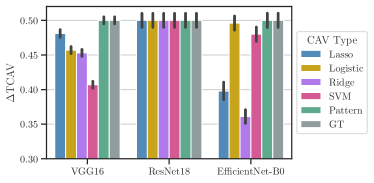
Figure 6: $\Delta\text{TCAV}$ (averaged over class-defining concepts) for different CAVs fitted on last Conv layers of VGG16, ResNet18, and EfficientNet-B0 trained on FunnyBirds. As models must use these concepts by experimental design, high scores are better. In contrast to filter-CAVs, pattern-CAVs achieve best scores for all models.

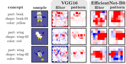
Figure 7: Visualization of concept-sensitivity maps, measured as element-wise product $\boldsymbol{\nabla}_{\mathbf{a}}\tilde{f}(\mathbf{a}(\mathbf{x}))\odot\mathbf{h}$ using filter- and pattern-CAVs for three concepts with VGG16 (middle) and EfficientNet-B0 (right). Results are shown for the last Conv layer, upsampled to input space dimensions. While pattern-CAVs precisely localize the concepts, filter-CAVs lead to noisy sensitivity maps.

4.3.2 CAV-based Model Correction (ClArC)

The ClArC framework [4] uses CAVs to model data artifacts in latent space to unlearn shortcuts, i.e., prediction strategies based on artifacts present in the training data with unintended relation to the task. Specifically, Right Reason ClArC (RR-ClArC) [15] is a recent approach that finetunes the model with an additional loss term $L_{\text{RR}}(\mathbf{x})=\left(\boldsymbol{\nabla}_{\mathbf{a}}\tilde{f}(\mathbf{a}(\mathbf{x}))\cdot\mathbf{h}\right)^{2}$. This loss term penalizes the use of latent features, measured via the gradient, pointing into the direction of CAV $\mathbf{h}$, representing the data artifact. An accurate estimated concept direction is crucial to ensure that the intended direction is penalized.

We correct the models trained in controlled settings with artificial shortcuts, namely ISIC2019 and Pediatric Bone Age with timestamp and color artifacts, respectively. We further correct models trained on ISIC2019 w.r.t. the known artifacts “band-aid”, “ruler”, and “skin marker” with artifact-specific CAVs. Training details are given in Appendix C.4.

Quantitative Evaluation

We evaluate the effectiveness of model correction by studying the impact of data poisoning on the model’s accuracy and its sensitivity to data artifacts. For the former, we measure the accuracy on a clean (artifact-free) and a biased test set, with the artifact inserted into all samples. For the real artifacts in ISIC2019, we automatically compute input localization masks [30] to cut (localizable) artifacts from known artifact samples and paste them onto test samples. To probe the model’s sensitivity to the artifact, we measure the fraction of relevance, computed with Layer-wise Relevance Propagation (LRP) [5], on the artifact region using our localization masks. Moreover, we compute the TCAV score after model correction using the sample-wise ground truth concept direction $\mathbf{h}^{\text{gt}}$. For real artifacts, the ground truth direction is computed for “attacked” samples $\textbf{x}_{\text{att}}$ with artificially inserted artifacts, as $\mathbf{h}_{\text{gt}}=\mathbf{a}(\mathbf{x}_{\text{att}})-\mathbf{a}(\mathbf{x})$. The model correction results for VGG16, ResNet18, and EfficientNet-B0 for ISIC2019 (timestamp artifact, controlled), Pediatric Bone Age (color artifact, controlled), and ISIC2019 (“band-aid” artifact, real) are shown in Table 1. We perform model correction for VGG16 after the 11^th and 12^th (out of 13) Conv layers in the controlled settings and for the “band-aid” artifact, respectively. ResNet18 and EfficientNet-B0 are corrected after the last Conv layer. We use filter-based (lasso, logistic, ridge regression, and SVM) and pattern-based CAVs as introduced in Eq. (3) to represent the direction to be unlearned. The models are finetuned and compared to a Vanilla model, which is trained without added loss term. Further training details are provided in Appendix B.2 and additional results, including standard errors, are provided in Appendix C.4. For VGG16, the accuracy on clean test sets remains largely unaffected, while pattern-CAVs outperform other methods in terms of accuracy on the biased test set. Moreover, pattern-CAVs yield best results for reduced artifact sensitivity, measured through artifact relevance and $\Delta\text{TCAV}^{\text{gt}}$. Similar artifact sensitivity results can be observed for ResNet18 and EfficientNet-B0. Furthermore, pattern-CAVs achieve the highest accuracies on biased test sets in the controlled settings. ResNet18 trained on Bone Age poses an exception, possibly due to other relevant signals correlated with the artifact direction. For the “band-aid” artifact, all CAVs yield similar accuracy scores on both clean and biased test sets. This can be attributed to the minimal impact of the artifact on EfficientNet-B0 and ResNet18, as indicated by the small accuracy difference between the two test sets. Additionally, the automated evaluation with estimated localization masks is error-prone. Lastly, Fig. 8 presents the accuracies on the biased test set for the two controlled datasets for model corrections on all VGG16 layers. Pattern-CAVs consistently achieve better scores across all layers close towards the end of the model output.

Table 1: Results after model correction with RR-ClArC for VGG16, ResNet18, and EfficientNet-B0 trained on Bone Age $|$ ISIC2019 (controlled) $|$ ISIC2019 (real). We report accuracy on clean and biased test set, the fraction of relevance put onto the data artifact region for localizable artifacts, and the TCAV score (reported as $\Delta\text{TCAV}^{\text{gt}}$) using the sample-wise ground-truth concept direction $\mathbf{h}^{\text{gt}}$, measuring the models’ sensitivity towards the artifacts after model correction. Arrows indicate whether low ($\downarrow$) or high ($\uparrow$) are better.

model	CAV	Accuracy (clean) $\uparrow$	Accuracy (biased) $\uparrow$	Artifact relevance $\downarrow$	$\Delta\text{TCAV}^{\text{gt}}$ $\downarrow$
VGG-16	Vanilla	${0.78}$ $\,|\,$ ${0.82}$ $\,|\,$ ${0.83}$	${0.50}$ $\,|\,$ ${0.28}$ $\,|\,$ ${0.75}$	- $\,|\,$ ${0.62}$ $\,|\,$ ${0.51}$	${0.29}$ $\,|\,$ ${0.14}$ $\,|\,$ ${0.10}$
	lasso	${0.77}$ $\,|\,$ ${0.82}$ $\,|\,$ ${0.82}$	${0.55}$ $\,|\,$ ${0.30}$ $\,|\,$ ${0.76}$	- $\,|\,$ ${0.60}$ $\,|\,$ ${0.49}$	${0.25}$ $\,|\,$ ${0.13}$ $\,|\,$ ${0.12}$
	logistic	${0.72}$ $\,|\,$ ${0.82}$ $\,|\,$ ${0.82}$	${0.63}$ $\,|\,$ ${0.37}$ $\,|\,$ ${0.78}$	- $\,|\,$ ${0.54}$ $\,|\,$ ${0.43}$	${0.25}$ $\,|\,$ $\mathbf{0.07}$ $\,|\,$ ${0.09}$
	ridge	${0.71}$ $\,|\,$ ${0.82}$ $\,|\,$ ${0.82}$	${0.61}$ $\,|\,$ ${0.31}$ $\,|\,$ ${0.76}$	- $\,|\,$ ${0.59}$ $\,|\,$ ${0.50}$	${0.24}$ $\,|\,$ ${0.13}$ $\,|\,$ ${0.12}$
	SVM	${0.69}$ $\,|\,$ ${0.81}$ $\,|\,$ ${0.82}$	${0.70}$ $\,|\,$ ${0.36}$ $\,|\,$ ${0.78}$	- $\,|\,$ ${0.55}$ $\,|\,$ ${0.46}$	${0.24}$ $\,|\,$ ${0.10}$ $\,|\,$ ${0.11}$
	Pattern (ours)	${0.78}$ $\,|\,$ ${0.80}$ $\,|\,$ ${0.82}$	$\mathbf{0.75}$ $\,|\,$ $\mathbf{0.69}$ $\,|\,$ $\mathbf{0.79}$	- $\,|\,$ $\mathbf{0.26}$ $\,|\,$ $\mathbf{0.31}$	$\mathbf{0.14}$ $\,|\,$ ${0.10}$ $\,|\,$ $\mathbf{0.03}$
ResNet-18	Vanilla	${0.76}$ $\,|\,$ ${0.84}$ $\,|\,$ ${0.84}$	${0.48}$ $\,|\,$ ${0.54}$ $\,|\,$ ${0.79}$	- $\,|\,$ ${0.30}$ $\,|\,$ ${0.26}$	${0.50}$ $\,|\,$ ${0.50}$ $\,|\,$ ${0.47}$
	lasso	${0.75}$ $\,|\,$ ${0.84}$ $\,|\,$ ${0.84}$	${0.69}$ $\,|\,$ ${0.54}$ $\,|\,$ $\mathbf{0.79}$	- $\,|\,$ ${0.29}$ $\,|\,$ $\mathbf{0.26}$	${0.50}$ $\,|\,$ ${0.50}$ $\,|\,$ ${0.47}$
	logistic	${0.73}$ $\,|\,$ ${0.83}$ $\,|\,$ ${0.84}$	$\mathbf{0.74}$ $\,|\,$ ${0.60}$ $\,|\,$ $\mathbf{0.79}$	- $\,|\,$ ${0.29}$ $\,|\,$ $\mathbf{0.26}$	${0.49}$ $\,|\,$ $\mathbf{0.49}$ $\,|\,$ ${0.46}$
	ridge	${0.77}$ $\,|\,$ ${0.83}$ $\,|\,$ ${0.84}$	${0.67}$ $\,|\,$ ${0.55}$ $\,|\,$ $\mathbf{0.79}$	- $\,|\,$ ${0.29}$ $\,|\,$ $\mathbf{0.26}$	${0.50}$ $\,|\,$ ${0.50}$ $\,|\,$ ${0.47}$
	SVM	${0.74}$ $\,|\,$ ${0.82}$ $\,|\,$ ${0.84}$	${0.73}$ $\,|\,$ ${0.59}$ $\,|\,$ $\mathbf{0.79}$	- $\,|\,$ ${0.29}$ $\,|\,$ $\mathbf{0.26}$	${0.50}$ $\,|\,$ $\mathbf{0.49}$ $\,|\,$ ${0.47}$
	Pattern (ours)	${0.75}$ $\,|\,$ ${0.76}$ $\,|\,$ ${0.83}$	${0.67}$ $\,|\,$ $\mathbf{0.73}$ $\,|\,$ $\mathbf{0.79}$	- $\,|\,$ $\mathbf{0.28}$ $\,|\,$ $\mathbf{0.26}$	$\mathbf{0.48}$ $\,|\,$ $\mathbf{0.49}$ $\,|\,$ $\mathbf{0.44}$
Efficient Net-B0	Vanilla	${0.79}$ $\,|\,$ ${0.87}$ $\,|\,$ ${0.87}$	${0.46}$ $\,|\,$ ${0.55}$ $\,|\,$ ${0.82}$	- $\,|\,$ ${0.55}$ $\,|\,$ ${0.37}$	${0.46}$ $\,|\,$ ${0.39}$ $\,|\,$ ${0.20}$
	lasso	${0.79}$ $\,|\,$ ${0.87}$ $\,|\,$ ${0.87}$	${0.47}$ $\,|\,$ ${0.55}$ $\,|\,$ $\mathbf{0.82}$	- $\,|\,$ ${0.55}$ $\,|\,$ ${0.37}$	${0.45}$ $\,|\,$ ${0.39}$ $\,|\,$ ${0.19}$
	logistic	${0.79}$ $\,|\,$ ${0.86}$ $\,|\,$ ${0.87}$	${0.48}$ $\,|\,$ ${0.54}$ $\,|\,$ $\mathbf{0.82}$	- $\,|\,$ ${0.55}$ $\,|\,$ ${0.37}$	${0.44}$ $\,|\,$ ${0.39}$ $\,|\,$ ${0.19}$
	ridge	${0.79}$ $\,|\,$ ${0.87}$ $\,|\,$ ${0.87}$	${0.49}$ $\,|\,$ ${0.55}$ $\,|\,$ $\mathbf{0.82}$	- $\,|\,$ ${0.55}$ $\,|\,$ ${0.37}$	${0.44}$ $\,|\,$ ${0.39}$ $\,|\,$ ${0.19}$
	SVM	${0.79}$ $\,|\,$ ${0.86}$ $\,|\,$ ${0.87}$	${0.50}$ $\,|\,$ ${0.54}$ $\,|\,$ $\mathbf{0.82}$	- $\,|\,$ ${0.55}$ $\,|\,$ ${0.37}$	${0.44}$ $\,|\,$ ${0.40}$ $\,|\,$ ${0.19}$
	Pattern (ours)	${0.74}$ $\,|\,$ ${0.86}$ $\,|\,$ ${0.84}$	$\mathbf{0.61}$ $\,|\,$ $\mathbf{0.61}$ $\,|\,$ ${0.79}$	- $\,|\,$ $\mathbf{0.52}$ $\,|\,$ $\mathbf{0.34}$	$\mathbf{0.37}$ $\,|\,$ $\mathbf{0.38}$ $\,|\,$ $\mathbf{0.14}$

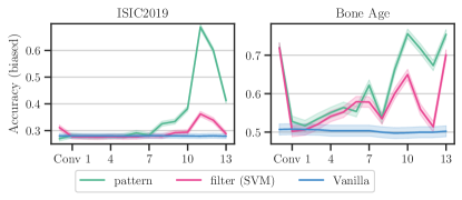
Figure 8: Accuracy on the biased test set for VGG16 trained on ISIC2019 (left) and Bone Age (right) and corrected with RR-ClArC with pattern- and filter-CAVs fitted on each Conv layer. Pattern-CAV consistently outperforms filter-CAV and corrections on layers closer to the model head.

Qualitative Evaluation

We compare attribution heatmaps for the Vanilla model with heatmaps for models corrected with RR-ClArC using filter- (SVM) and pattern-based CAVs w.r.t. the band-aid, ruler, and skin marker artifacts using the VGG16 model trained on ISIC2019 in Fig. 9. In addition to the traditional attribution heatmap computed with LRP using the $\varepsilon z^{+}\flat$-composite [26] in zennit [3], we show another heatmap highlighting the difference between the normalized relevance heatmaps of the corrected and the Vanilla model, with blue and red showing areas with lower and higher relevance after correction, respectively. Pattern-based CAVs reduce the relevance of data artifacts after model correction significantly, while traditional SVM-CAVs only have little impact. Additional examples are shown in Appendix C.4.

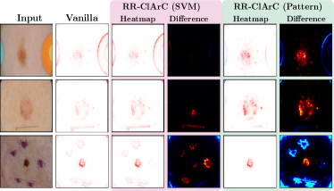
Figure 9: Qualitative results for model correction w.r.t. real artifacts band-aid (top), ruler (middle), and skin marker (bottom) in ISIC2019 using VGG16. In addition to attribution heatmaps for models corrected with filter- (SVM) and pattern-CAVs, we show heatmaps highlighting the differences compared to the Vanilla model attribution heatmap, with red and blue indicating higher and lower relevance after correction, respectively. Whereas filter-CAVs have limited impact, pattern-CAVs successfully increases the relevance on the mole and decreases the relevance on data artifacts.

4.3.3 Limitations

Our results confirm that pattern-CAVs exhibit superior alignment with ground truth concept directions compared to filter-CAVs. This has a positive impact on CAV applications that heavily rely on precise concept directions, such as concept sensitivity testing with TCAV and model correction with ClArC. However, for CAV applications in which class-separability is more important, i.e., determining whether a concept is present in a given sample, filter-based CAVs might be a better choice. For instance, post-hoc concept bottleneck models [42] project latent embeddings into an interpretable concept space spanned by CAVs and fit a linear classifier in the resulting concept space. The linear classifier can handle directional divergence in CAVs and is rather reliant on a precise decision hyperplane, making filter-based CAVs superior in such scenarios. Thus, the choice of CAV computation methods should be carefully considered based on the specific task at hand.

5 Conclusion

While filters from linear classifiers can accurately predict the presence of concepts, they fall short in precisely modeling the direction of the concept signal. As many applications of CAVs, including TCAV and ClArC, heavily rely on accurate concept directions, we address this drawback by introducing pattern-based CAVs, which disregard distractor signals and focus solely on the concept signal. We provide both theoretical and empirical evidence to support the improved estimation of the true concept direction compared to widely used filter-based CAVs. Furthermore, we demonstrate the positive impact on applications leveraging CAVs, such as estimating the model’s sensitivity towards concepts and correcting model shortcut behavior caused by data artifacts. Future research might explore the optimization of concept directions beyond binary labels and the disentanglement of correlated concept directions.

Appendix

Appendix A Methods

In the following, we provide additional details and proofs related to our methods. Specifically, we provide details for linear models considered for filter-based CAVs in Section A.1, prove the robustness to noise and scaling of pattern-CAVs in Section A.2, and further prove that in case of binary target labels the pattern is equivalent to the difference of cluster means in Section A.3. Moreover, we present additional 2D toy experiments in Section A.4 and provide proofs of divergence for filter-based approaches in Section A.5 and Section A.6 for feature scaling and noise rotation, respectively.

A.1 Details for filter-based CAV approaches

We briefly summarize the optimization objectives for linear models for filter-based CAV approaches, including lasso, logistic, and ridge regression, as well as SVM s. All methods aim to find a hyperplane that separates a dataset ${\mathcal{X}\subset\mathbb{R}^{m}}$ of size $n$ into two sets, defined by concept label $t\in\{+1,-1\}$. This is achieved by fitting a weight vector $\mathbf{w}\in\mathbb{R}^{m}$ and a bias $b\in\mathbb{R}$ such that the hyperplane consists of all $\mathbf{x}$ which satisfy $\mathbf{w}^{\top}\mathbf{x}+b=0$.

Lasso regression [37] aims to minimize residuals $r_{i}=\left(t_{i}-(\mathbf{w}^{\top}\mathbf{x}_{i}+b)\right)$ with $L_{1}$-norm regularization, thereby encouraging sparse coefficients. The optimization problem is given by

$$\min_{\mathbf{w},b}\left\{\frac{1}{n}\sum_{i\in[n]}r_{i}^{2}+\lambda\sum_{j\in[m]}|w_{j}|\right\}~{}.$$ (7)

Similarly, ridge regression [23] fits a linear model which minimizes the residuals $r_{i}$ with $L_{2}$-norm regularization by solving

$$\min_{\mathbf{w},b}\left\{\frac{1}{n}\sum_{i\in[n]}r_{i}^{2}+\lambda\sqrt{\sum_{j\in[m]}w_{j}^{2}}\right\}~{}.$$ (8)

The logistic regression model estimates probabilities via

$$\widehat{\mathbb{P}}_{\mathbf{w},b}(t=+1\mid\mathbf{x})=\frac{e^{\mathbf{w}^{\top}\mathbf{x}+b}}{1+e^{\mathbf{w}^{\top}\mathbf{x}+b}}=\sigma(\mathbf{w}^{\top}\mathbf{x}+b),$$

where $\sigma$ denotes the sigmoid function $\sigma(z)=\frac{e^{z}}{1+e^{z}}$. The linear model is now fitted by maximizing the log likelihood of the observed data:

$$\begin{split}&\max_{\mathbf{w},b}L(\mathbf{w},b;\mathcal{X})\\ &=\max_{\mathbf{w},b}\sum_{i\in[n]}\mathbbm{1}(t_{i}=+1)\log\widehat{\mathbb{P}}_{\mathbf{w},b}(t=+1\mid\mathbf{x}_{i})\\ &\qquad\qquad\ +\mathbbm{1}(t_{i}=-1)\log\left(1-\widehat{\mathbb{P}}_{\mathbf{w},b}(t=+1\mid\mathbf{x}_{i})\right).\end{split}$$ (9)

Lastly, and most commonly used for CAVs, SVMs [12] fit a linear model by finding a hyperplane that maximizes the margin between two classes using the hinge loss, defined as $l_{i}=\max\left(0,1-t_{i}\left(\mathbf{w}^{\top}\mathbf{x}_{i}+b\right)\right)$ and $L_{2}$-norm regularization with the following optimization objective:

$$\min_{\mathbf{w},b}\left\{\frac{1}{n}\sum_{i\in[n]}l_{i}+\lambda\sqrt{\sum_{j\in[m]}w_{j}^{2}}\right\}~{}.$$ (10)

A.2 Feature Scaling and Noise on Pattern-CAV

In this section, we investigate the effect of feature scaling and additive noise on the resulting pattern-CAV. We start from the known solution for a simple linear regression task provided in Equation 3, resulting in a pattern-CAV of

$$\begin{split}\mathbf{h}^{\text{pat}}&=\frac{\text{cov}[\mathcal{A},t]}{\sigma_{t}^{2}}.\end{split}$$ (11)

Feature Scaling

We start with the effect of feature scaling on $\mathbf{h}^{\text{pat}}$. Specifically, we investigate the effect on the CAV, when we scale a specific dimension $k$ of features $\mathbf{a}\in\mathbb{R}^{m}$ (of dimension $m$) with a factor $\gamma$, i.e.,

$$a^{\gamma}_{i}=\begin{cases}a_{i},&i\neq k\\ \gamma a_{i}&i=k.\end{cases}$$ (12)

Then, with Eq. (11), we get for the corresponding pattern-CAV

$$\begin{split}{(h^{\gamma})}^{\text{pat}}_{i}&=\frac{1}{\sigma_{t}^{2}|\mathcal{X}|}\sum_{\mathbf{x},t\in\mathcal{X}_{\mathbf{h}}}(a_{i}^{\gamma}(\mathbf{x})-\bar{a}_{i}^{\gamma})(t-\bar{t})\\ &=\begin{cases}{h}^{\text{pat}}_{i}\,\text{if}\,i\neq k\\ \gamma{h}^{\text{pat}}_{i}\,\text{if}\,i=k.\end{cases}\\ \end{split}$$ (13)

meaning that the CAV $\mathbf{h}^{\text{pat}}$ scales with the features (contrary to many classification-based CAVs).

Additive Noise

We add random noise $\epsilon$ with zero mean $\mathbb{E}[\epsilon]=0$, that is independent to the concept labels $t$ to a feature dimension $k$. Then in expectation

$$\begin{split}\mathbb{E}[{h^{\prime}}^{\text{pat}}_{i}]&=\frac{1}{\sigma_{t}^{2}}\mathbb{E}[(a_{i}-\bar{a}_{i}+\delta_{ik}\epsilon)(t-\bar{t})]\\ &=\frac{1}{\sigma_{t}^{2}}\left[\mathbb{E}[(a_{i}-\bar{a}_{i})(t-\bar{t})]+\mathbb{E}[\epsilon_{k}(t-\bar{t})]\right]\\ &=\frac{1}{\sigma_{t}^{2}}\mathbb{E}[(a_{i}-\bar{a}_{i})(t-\bar{t})]={h}^{\text{pat}}_{i},\end{split}$$ (14)

where we used the independence of $\epsilon$ and $t$, i.e., $\mathbb{E}[\epsilon t]=\mathbb{E}[\epsilon]t=0$.

A.3 Pattern-CAV Reducing to the Difference of Means

Assuming for easier notation we have binary concept labels $t\in\{0,1\}$. We start from Eq. (3) for the pattern-CAV, given by the known solution for a simple linear regression task given as

$$\begin{split}\mathbf{h}^{\text{pat}}&=\frac{\text{cov}[\mathcal{A},t]}{\sigma_{t}^{2}}.\end{split}$$ (15)

For the covariance term, we get

$$\begin{split}\text{cov}[\mathcal{A},t]&=\frac{1}{|\mathcal{X}_{\mathbf{h}}|}\sum_{\mathbf{x},t\in\mathcal{X}_{\mathbf{h}}}(\mathbf{a}(\mathbf{x})-\bar{\mathcal{A}})(t-\bar{t})\\ &=\frac{1}{|\mathcal{X}_{\mathbf{h}}|}\left[\sum_{\mathbf{x},t\in\mathcal{X}_{\mathbf{h}}^{+}}(\mathbf{a}(\mathbf{x})-\bar{\mathcal{A}})(1-\bar{t})\right.\\ &\left.\quad-\sum_{\mathbf{x},t\in\mathcal{X}_{\mathbf{h}}^{-}}(\mathbf{a}(\mathbf{x})-\bar{\mathcal{A}})\bar{t}\right]\end{split}$$ (16)

We have $|\mathcal{X}_{\mathbf{h}}^{+}|$ positive (with concept) sample activations $\mathcal{A}^{+}$ and $|\mathcal{X}_{\mathbf{h}}^{-}|$ negative (without concept) sample activations $\mathcal{A}^{-}$. We further introduce $\alpha^{\pm}=\frac{|\mathcal{X}_{\mathbf{h}}^{\pm}|}{|\mathcal{X}_{\mathbf{h}}^{|}}$, therefore, $\bar{t}=\alpha^{+}$ and $1-\bar{t}=\alpha^{-}$ using $t\in\{0,1\}$. Thus, we can write

$$\begin{split}\text{cov}[\mathcal{A},t]&=\frac{1}{|\mathcal{X}_{\mathbf{h}}|}\left[\alpha^{-}\sum_{\mathbf{x},t\in\mathcal{X}_{\mathbf{h}}^{+}}(\mathbf{a}(\mathbf{x})-\bar{\mathcal{A}})\right.\\ &\left.\quad-\alpha^{+}\sum_{\mathbf{x},t\in\mathcal{X}_{\mathbf{h}}^{-}}(\mathbf{a}(\mathbf{x})-\bar{\mathcal{A}})\right]\\ &=\frac{1}{|\mathcal{X}_{\mathbf{h}}|}\left[\alpha^{-}p(\bar{\mathcal{A}}^{+}-\bar{\mathcal{A}})-\alpha^{+}n(\bar{\mathcal{A}}^{-}-\bar{\mathcal{A}})\right],\end{split}$$ (17)

where we used for the last step that

$$\bar{\mathcal{A}}^{\pm}=\frac{1}{|\mathcal{X}_{\mathbf{h}}^{\pm}|}\sum_{\mathbf{x},t\in\mathcal{X}_{\mathbf{h}}^{\pm}}\mathbf{a}(\mathbf{x}).$$ (18)

Finally, we receive

$$\text{cov}[\mathcal{A},t]=\frac{|\mathcal{X}_{\mathbf{h}}^{+}||\mathcal{X}_{\mathbf{h}}^{-}|}{|\mathcal{X}_{\mathbf{h}}|^{2}}(\bar{\mathcal{A}}^{+}-\bar{\mathcal{A}}^{-})={\sigma_{t}^{2}}(\bar{\mathcal{A}}^{+}-\bar{\mathcal{A}}^{-})$$ (19)

and

$$\mathbf{h}^{\text{pat}}=\bar{\mathcal{A}}^{+}-\bar{\mathcal{A}}^{-}.$$ (20)

A.4 2D Toy Examples

In addition to the 2D experiments conducted in Section 3.3 in the main paper, we investigate two more scenarios in which we (1) increase the standard deviation and (2) vary the random seed. For the former, we randomly sample data points for class A from $\mathcal{N}((0~{}1)^{\top},\Sigma)$ and for class B from $\mathcal{N}((5~{}1)^{\top},\Sigma)$ with $\Sigma=\begin{pmatrix}\sigma^{2}&0\\ 0&\sigma^{2}\end{pmatrix}$ and incrementally increase $\sigma$. For the latter, we sample from the same distributions with fixed $\sigma=1$, but use different random seeds for each run. We fit both pattern- and filter-CAVs for both experiments. As filter, we use a hard-margin SVMs. Fig. 10 presents results for additional runs for the settings discussed in the main paper, namely noise rotation (1^st row) and feature scaling (2^nd row), as well as the new 2D settings, including increased standard deviation (3^rd row) and different random seeds (4^th row). In addition to the observations discussed in the main paper, we can see that filter-CAVs from hard-margin SVMs diverge for increased values for $\sigma$, as samples are not perfectly separable anymore. Moreover, the filter-CAVs is sensitive to random seeds. In contrast, pattern-CAVs constantly point into the correct direction for all settings. Animated visualizations for all challenges discussed can be found here: http://tinyurl.com/ymywcwmo.

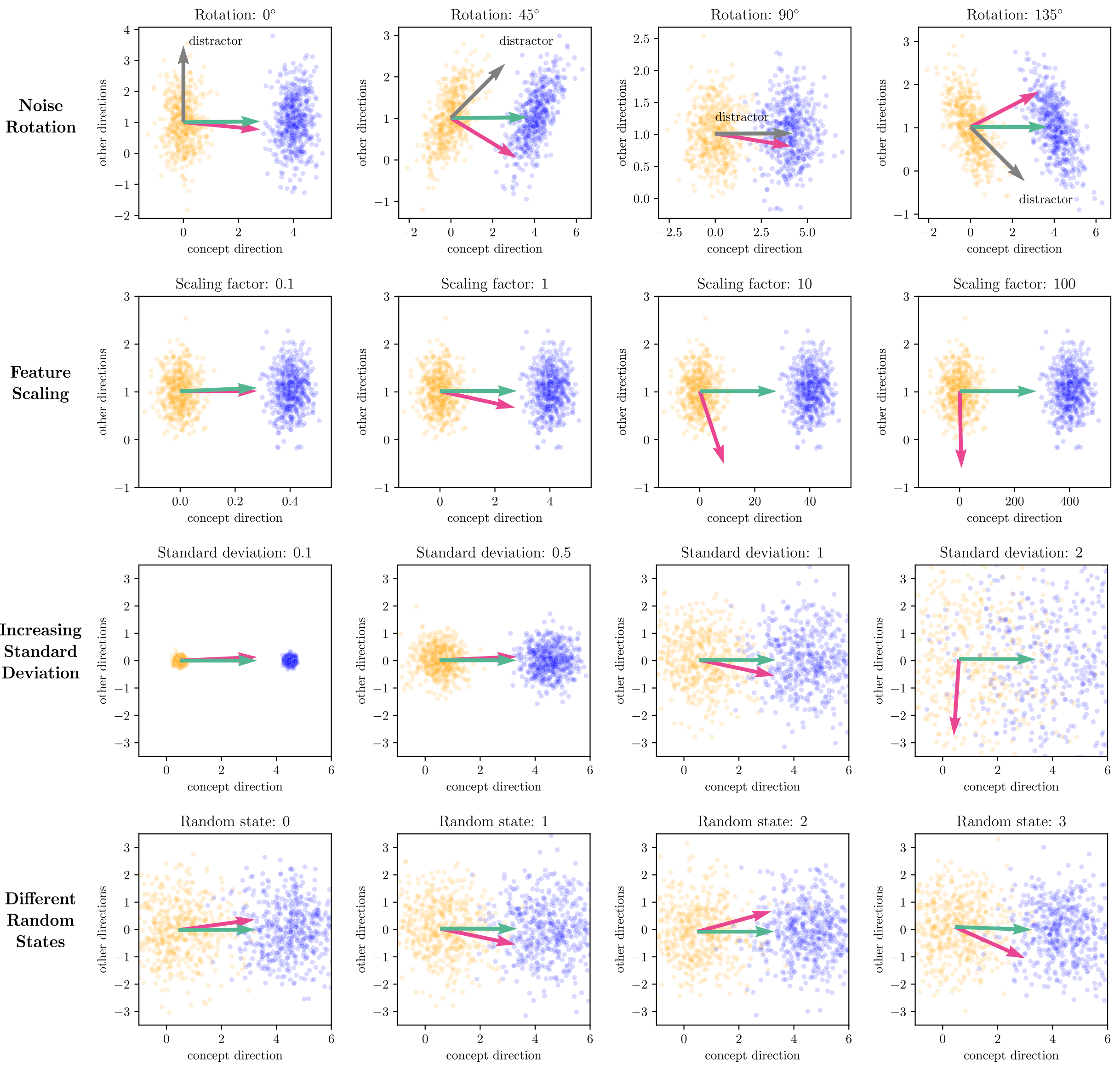
Figure 10: Multiple runs for 2D toy experiments. For noise rotation (1^st row), the filter-CAV (magenta) diverges depending on the distractor direction, while pattern-CAV (green) stays constant. When increasing the scale of the x-axis (2^nd row), the filter CAV scales antiproportional. For increased standard deviation (3^rd row), filter-CAVs (here: hard-margin SVM) diverge when the clusters are not perfectly separable anymore. Lastly, different random seeds for not perfectly separable clusters lead to varying directions for filter-based CAVs (4^th row).

A.5 Proof of divergence: Scaling

We consider the general case of logistic regression on a set of activations $\mathcal{A}\subset\mathbb{R}^{m}$. For a weight vector $\mathbf{w}\in\mathbb{R}^{m}$ and bias term $b\in\mathbb{R}$ logistic regression models the probability of an activation $\mathbf{a}$ corresponding to concept label $t=+1$ as

$$\widehat{\mathbb{P}}_{\mathbf{w},b}(t=+1\mid\mathbf{a})=\frac{e^{\mathbf{w}^{\top}\mathbf{a}+b}}{1+e^{\mathbf{w}^{\top}\mathbf{a}+b}}=\sigma(\mathbf{w}^{\top}\mathbf{a}+b),$$ (21)

where $\sigma$ denotes the sigmoid function $\sigma(z)=\frac{e^{z}}{1+e^{z}}$. We predict $t=+1$ for an activation $\mathbf{a}$ if ${\widehat{\mathbb{P}}_{\mathbf{w},b}(t=+1\mid\mathbf{a})>0.5}$ and $t=-1$ otherwise. To train an unpenalized logistic regression classifier, we seek to maximize the log likelihood of our observed activations $\mathcal{A}$

$$\begin{split}&L(\mathbf{w},b;\mathcal{A})\\ &=\sum_{i\in[n]}\mathbbm{1}(t_{i}=+1)\log\widehat{\mathbb{P}}_{\mathbf{w},b}(t=+1\mid\mathbf{a}_{i})\\ &\qquad+\mathbbm{1}(t_{i}=-1)\log\left(1-\widehat{\mathbb{P}}_{\mathbf{w},b}(t=+1\mid\mathbf{a}_{i})\right).\end{split}$$ (22)

Assume for our unscaled set $\mathcal{A}$, we have found an optimal choice

$$\widehat{\mathbf{w}},\hat{b}\in\underset{\mathbf{w}\in\mathbb{R}^{m},b\in\mathbb{R}}{\operatorname{argmax}}L(\mathbf{w},b;\mathcal{A}).$$ (23)

To introduce the scaling along an axis, for a given vector $\mathbf{a}\in\mathbb{R}^{n}$ and a dimension $k\in[n]$ we denote by $\mathbf{a}^{\gamma}$ the vector which has the same entries as $\mathbf{a}$ except for the $k$-th entry, which has been replaced by $\gamma a_{k}$. Further, let ${\mathcal{A}^{\gamma}=\{\mathbf{a}^{\gamma}\mid\mathbf{a}\in\mathcal{A}\}}$ denote the set of scaled activations. Finally, for the weight vector $\mathbf{w}$ we introduce the equivalent notation $\mathbf{w}^{1/\gamma}$ for the vector in which only the $k$-th entry of $\mathbf{w}$ has been changed to $\frac{1}{\gamma}w_{k}$. Then we derive the following equality

$$\begin{split}&\left({\mathbf{w}^{1/\gamma}}\right)^{\top}\mathbf{a}^{\gamma}+b\\ &=w_{1}a_{1}+\ldots+\left(\frac{1}{\gamma}w_{k}\right)\left(\gamma a_{k}\right)+\ldots+w_{m}a_{m}+b\\ &=\mathbf{w}^{\top}\mathbf{a}+b,\end{split}$$ (24)

which implies the equalities of the predicted probabilities

$${\widehat{\mathbb{P}}_{\mathbf{w}^{1/\gamma},b}(t=+1\mid\mathbf{a}^{\gamma})}={\widehat{\mathbb{P}}_{\mathbf{w},b}(t=+1\mid\mathbf{a})}$$ (25)

and thus of the log likelihoods

$$L(\mathbf{w}^{1/\gamma},b;\mathcal{A}^{\gamma})=L(\mathbf{w},b;\mathcal{A}).$$ (26)

Therefore it follows that the optimal solution to logistic regression on the scaled dataset relates to our original solution on the unscaled dataset via

$$\widehat{\mathbf{w}}^{1/\gamma},\hat{b}=\underset{\mathbf{w}\in\mathbb{R}^{m},b\in\mathbb{R}}{\operatorname{argmax}}L(\mathbf{w},b;\mathcal{A}^{\gamma}).$$ (27)

In conclusion, scaling the activations by a factor of $\gamma$ in one dimension leads the signal to also scale by factor of $\gamma$ in this dimension. The filter-based CAV calculated as the weight vector of an unpenalized logistic regression, however, exhibits a scaling in the same dimension which is antiproportional to the scaling factor $\gamma$. Such antipropotional scaling will misalign the filter-based CAV unless it is either perfectly aligned or perfectly orthogonal to the direction of scaling. This shows that even if the filter-based CAV theoretically lies aligned or orthogonal to the scaling dimension due to noise and constraints in machine precision, logistic regression may be hugely affected by the lack of feature scaling.

A.6 Proof of divergence: Noise rotation

With the additional rotational noise term and assuming the concept label $t_{i}$ to be fixed, our activations $A_{i}$ are distributed according to independent multivariate normal distributions $\mathcal{N}(\mu_{i},\Sigma)$ with

$$\begin{split}\mu_{i}&=\begin{pmatrix}1\\ 0\end{pmatrix}\mathbbm{1}(t_{i}=+1),\\ \Sigma&=\begin{pmatrix}\sigma^{2}+\sin^{2}\tau&\sin\tau\cos\tau\\ \sin\tau\cos\tau&\sigma^{2}+\cos^{2}\tau\end{pmatrix}.\end{split}$$ (28)

From this formulation we can see that this adds a noise which is correlated in the direction parallel and orthogonal to the CAVs, unless $\tau$ is a multiple of $\frac{\pi}{2}$ in which case we only add noise parallel or orthogonal to the CAVs respectively. It thus follows that the random variable $\mathbf{w}^{\top}A_{i}+b$ has the following distribution:

$$\mathbf{w}^{\top}A_{i}+b\stackrel{{\scriptstyle ind.}}{{\sim}}\mathcal{N}\left(w_{1}\mathbbm{1}(t_{i}=+1)+b,\mathbb{V}(\mathbf{w}^{\top}A_{i})\right).$$ (29)

Note that the choice of $w_{2}$ does not affect the expected value of $\mathbf{w}^{\top}A_{i}+b$ but may change its variance. To study this effect on the variance, for a given $\lambda\neq 0$ define the family of weight vectors

$$\mathcal{W}_{\lambda}=\left\{\lambda\begin{pmatrix}1\\ w_{2}\end{pmatrix}\;\middle|\;w_{2}\in\mathbb{R}\right\}.$$ (30)

Theorem A.1.

Define the vector $\widetilde{\mathbf{w}}_{\lambda}=\lambda\begin{pmatrix}1\\ \widetilde{w}_{2}\end{pmatrix}$ where $\widetilde{w}_{2}=-\frac{\sin\tau\cos\tau}{\sigma^{2}+\cos^{2}\tau}$. Then $\widetilde{\mathbf{w}}_{\lambda}$ is the unique minimizer

$$\widetilde{\mathbf{w}}_{\lambda}=\underset{\mathbf{w}\in\mathcal{W}_{\lambda}}{\operatorname{argmin}}\ \mathbb{V}(\mathbf{w}^{\top}A_{i}).$$ (31)

Proof.

The variance for $\mathbf{w}\in\mathcal{W}_{\lambda}$ is given by

$$\begin{split}&\mathbb{V}(\mathbf{w}^{\top}A_{i})\\ &=\lambda^{2}\begin{pmatrix}1&w_{2}\end{pmatrix}\begin{pmatrix}\sigma^{2}+\sin^{2}\tau&\sin\tau\cos\tau\\ \sin\tau\cos\tau&\sigma^{2}+\cos^{2}\tau\end{pmatrix}\begin{pmatrix}1\\ w_{2}\end{pmatrix}\\ &=\lambda^{2}\left\{\sigma^{2}+\sin^{2}\tau+2w_{2}\sin\tau\cos\tau+w_{2}^{2}\sigma^{2}+w_{2}^{2}\cos^{2}\tau\right\}\\ &=\lambda^{2}\left\{\sigma^{2}+w_{2}^{2}\sigma^{2}+(\sin\tau+w_{2}\cos\tau)^{2}\right\}.\end{split}$$ (32)

Differentiating with respect to $w_{2}$ gives the following expression

$$\begin{split}\frac{\partial}{\partial w_{2}}\mathbb{V}(\mathbf{w}^{\top}A_{i})=&\lambda^{2}\left\{2w_{2}\sigma^{2}+2\cos\tau(\sin\tau+w_{2}\cos\tau)\right\}\\ =&2\lambda^{2}\left\{(\sigma^{2}+\cos^{2}\tau)w_{2}+\sin\tau\cos\tau\right\}\end{split}$$ (33)

This is set to zero if and only if $\widetilde{w}_{2}=-\frac{\sin\tau\cos\tau}{\sigma^{2}+\cos^{2}\tau}$. Furthermore, the second derivative is

$$\frac{\partial^{2}}{\partial w_{2}^{2}}\mathbb{V}(\mathbf{w}^{\top}A_{i})=2\lambda^{2}\left(\sigma^{2}+\cos^{2}\tau\right)>0,$$ (34)

so $\widetilde{w}_{2}$ indeed minimizes the variance. ∎

The proofs of divergence for both logistic regression and SVMs are now analogous: Assuming there are two vectors $\mathbf{w},\widetilde{\mathbf{w}}$ for which $\mathbf{w}^{\top}A_{i}+b$ has the same expected value but $\widetilde{\mathbf{w}}$ yields a smaller variance, then the expected value of the objective function of the optimization problem of the model (the log likelihood for logistic regression or the size of the margin for SVMs respectively) will be larger for $\widetilde{\mathbf{w}}$. Together with Theorem A.1, this proves that a vector of the form $\widetilde{\mathbf{w}}_{\lambda}$ maximizes the expected value of the objective function and is thus preferred as the weight vector over the true CAV $(1~{}~{}0)^{\top}$ with non-zero probability.

A.6.1 Logistic Regression

For logistic regression, we intend to maximize the log likelihood of our observed data. We may express our log likelihood in terms of the random variables $\mathbf{w}^{\top}A_{i}+b$ by the formula

$$L(\mathbf{w},b;\mathcal{A}) =\sum_{i\in[N]} \mathbbm{1}(t_{i}=+1)\log(\sigma(\mathbf{w}^{\top}A_{i}+b))$$ (35)

$$+ \mathbbm{1}(t_{i}=-1)\log(1-\sigma(\mathbf{w}^{\top}A_{i}+b))$$

$$=\sum_{i\in[N]} \mathbbm{1}(t_{i}=+1)\log(\sigma(\mathbf{w}^{\top}A_{i}+b))$$

$$+ \mathbbm{1}(t_{i}=-1)\log(\sigma(-\mathbf{w}^{\top}A_{i}-b)),$$

where $\sigma$ denotes the sigmoid function.

Theorem A.2.

Let $\mathbf{w},\widetilde{\mathbf{w}}$ be two weight vectors with $\mathbb{E}\left[\mathbf{w}^{\top}A_{i}+b\right]=\mathbb{E}\left[\widetilde{\mathbf{w}}^{\top}A_{i}+b\right]$ for all $i\in[n]$ and $\mathbb{V}(\mathbf{w}^{\top}A_{i}+b)>\mathbb{V}(\widetilde{\mathbf{w}}^{\top}A_{i}+b)$. Then

$$\mathbb{E}\left[L(\widetilde{\mathbf{w}},b;\mathcal{A})\right]>\mathbb{E}\left[L(\mathbf{w},b;\mathcal{A})\right].$$ (36)

Proof.

To focus on the effect of the variance on the log likelihood, we define independently distributed random variables $Y_{i}\sim\mathcal{N}(\mu_{i},\varsigma^{2})$ with means $\mu_{i}$ and shared variance $\varsigma^{2}>0$. We allow the $Y_{i}$ to have different means as the mean of the random variables $\mathbf{w}^{\top}A_{i}+b$ also differ depending on the concept label $t_{i}$. We may now define the functions $f$ and $g_{i}$ which both depend on $\varsigma^{2}$ via

$$g_{i}(Y_{i})=\mathbbm{1}(t_{i}=+1)\log(\sigma(Y_{i}))+\mathbbm{1}(t_{i}=-1)\log(\sigma(-Y_{i}))$$ (37)

and

$$\begin{split}f(\varsigma^{2})=\mathbb{E}\left[\sum_{i\in[n]}g_{i}(Y_{i})\right]=\sum_{i\in[n]}\mathbb{E}\left[g_{i}(Y_{i})\right],\end{split}$$ (38)

where we used the linearity of the expected value in the last step. After proving that the function $f$ is strictly decreasing the claim follows from inserting $\mathbf{w}^{\top}A_{i}+b$ for $Y_{i}$. We prove first that $\log(\sigma(z))$ is a strictly concave function by calculating the second derivative:

$$\begin{split}(\log(\sigma(z)))^{\prime\prime}&=\left(\frac{1}{\sigma(z)}\sigma(z)(1-\sigma(z))\right)^{\prime}=\left(1-\sigma(z)\right)^{\prime}\\ &=-\sigma(z)(1-\sigma(z))<0\text{ for }z\in\mathbb{R}\end{split}$$ (39)

as the image of the sigmoid function is the open interval $(0,1)$. Because the logarithm of the sigmoid is a strictly concave function, so is $\log(\sigma(-z))$, hence each summand

$$\begin{split}g_{i}(Y_{i})&=\mathbbm{1}(t_{i}=+1)\log(\sigma(Y_{i}))\\ &+\mathbbm{1}(t_{i}=-1)\log(\sigma(-Y_{i}))\end{split}$$ (40)

is strictly concave in $Y_{i}$.
Now consider two variances $\varsigma_{1}^{2}<\varsigma_{2}^{2}$ and define independent random variables $Y_{i}^{1}\sim\mathcal{N}(\mu_{i},\varsigma_{1}^{2})$ and $Y_{i}^{\prime}\sim\mathcal{N}(0,\varsigma_{2}^{2}-\varsigma_{1}^{2})$ such that their sum are independently distributed random variables $Y_{i}^{2}:=Y_{i}^{1}+Y_{i}^{\prime}\sim\mathcal{N}(\mu_{i},\varsigma_{2}^{2})$. Using the conditional version of Jensen’s inequality on the strictly concave functions $g_{i}$, we derive

$$\begin{split}\mathbb{E}\left[g_{i}(Y_{i}^{2})\right]&=\mathbb{E}\left[g_{i}(Y_{i}^{1}+Y_{i}^{\prime})\right]\\ &=\mathbb{E}\left[\mathbb{E}\left[g_{i}(Y_{i}^{1}+Y_{i}^{\prime})\mid Y_{i}^{1}\right]\right]\\ &<\mathbb{E}\left[g_{i}\left(\mathbb{E}\left[Y_{i}^{1}+Y_{i}^{\prime}\mid Y_{i}^{1}\right]\right)\right]\\ &=\mathbb{E}\left[g_{i}\left(Y_{i}^{1}+\mathbb{E}\left[Y_{i}^{\prime}\right]\right)\right]\\ &=\mathbb{E}\left[g_{i}\left(Y_{i}^{1}\right)\right],\end{split}$$ (41)

where the second-to-last step follows from the properties of conditional expectation for completely dependent and independent random variables. Summing over all $i$ finally proves the desired inequality

$$f(\varsigma_{1}^{2})=\sum_{i\in[n]}\mathbb{E}\left[g_{i}\left(Y_{i}^{1}\right)\right]>\sum_{i\in[n]}\mathbb{E}\left[g_{i}\left(Y_{i}^{2}\right)\right]=f(\varsigma_{2}^{2}).$$ (42)

∎

A.6.2 SVMs

We inspect the behavior of a linear hard-margin SVM, assuming that our data can be perfectly separated by a linear hyperplane. Then the optimization problem for this particular SVM is given by

$$\begin{split}\max_{\mathbf{w},b}&\frac{2}{\|\mathbf{w}\|_{2}}\\ \text{subject to }&t_{i}(\mathbf{w}^{\top}A_{i}+b)\geq 1\text{ for all }i\in[n].\end{split}$$ (43)

This states that we aim to maximize the margin which has length $2/\|\mathbf{w}\|_{2}$ subject to every datapoint lying on the correct side of the margin. A fitted SVM will have at least one vector of each class, the so-called support vectors, on its margin, which can be equally formulated as ${\min_{t_{i}=+1}\left(\mathbf{w}^{\top}A_{i}+b\right)=1}$ and ${\max_{t_{i}=-1}\left(\mathbf{w}^{\top}A_{i}+b\right)=-1}$. We may use these quantities to reformulate the length of the margin as

$$\frac{1}{\|\mathbf{w}\|_{2}}\left\{\min_{t_{i}=+1}\left(\mathbf{w}^{\top}A_{i}+b\right)-\max_{t_{i}=-1}\left(\mathbf{w}^{\top}A_{i}+b\right)\right\},$$ (44)

which is what we are trying to maximize in order to find the direction of our weight vector $\mathbf{w}$.

Theorem A.3.

Let $\mathbf{w},\widetilde{\mathbf{w}}$ be two weight vectors with $\mathbb{E}\left[\mathbf{w}^{\top}A_{i}+b\right]=\mathbb{E}\left[\widetilde{\mathbf{w}}^{\top}A_{i}+b\right]$ for all $i\in[n]$, ${\mathbb{V}(\mathbf{w}^{\top}A_{i}+b)>\mathbb{V}(\widetilde{\mathbf{w}}^{\top}A_{i}+b)}$ and $\|\mathbf{w}\|_{2}\leq\|\widetilde{\mathbf{w}}\|_{2}$. Then for sufficiently large sample size $n$ the expected margin size for the SVM with normal vector in direction of $\widetilde{\mathbf{w}}$ is bigger than for the SVM with normal vector in direction of $\mathbf{w}$.

Proof.

We denote $\mu_{+}=\mathbb{E}\left[\mathbf{w}^{\top}A_{i}+b\mid t_{i}=+1\right]$, ${\mu_{-}=\mathbb{E}\left[\mathbf{w}^{\top}A_{i}+b\mid t_{i}=-1\right]}$ and $\varsigma^{2}=\mathbb{V}\left(\mathbf{w}^{\top}A_{i}+b\right)$, and further define random variables $N_{i},N_{i}^{\prime}$ as independent standard normal distributions. We can now write the expected size of the margin as

$$\begin{split}\mathbb{E}&\left[\frac{1}{\|\mathbf{w}\|_{2}}\left\{\min_{t_{i}=+1}\left(\mathbf{w}^{\top}A_{i}+b\right)-\max_{t_{i}=-1}\left(\mathbf{w}^{\top}A_{i}+b\right)\right\}\right]\\ &=\frac{1}{\|\mathbf{w}\|_{2}}\left\{\mu_{+}-\mu_{-}+\varsigma\mathbb{E}\left[\min_{i\in[n/2]}N_{i}-\max_{i\in[n/2]}N_{i}^{\prime}\right]\right\}\\ &=\frac{1}{\|\mathbf{w}\|_{2}}\left\{\mu_{+}-\mu_{-}-\varsigma\mathbb{E}\left[\max_{i\in[n/2]}N_{i}+\max_{i\in[n/2]}N_{i}^{\prime}\right]\right\}\\ &=\frac{1}{\|\mathbf{w}\|_{2}}\left\{\mu_{+}-\mu_{-}-2\varsigma\mathbb{E}\left[\max_{i\in[n/2]}N_{i}\right]\right\}\\ &=\frac{1}{\|\mathbf{w}\|_{2}}\left\{\mu_{+}-\mu_{-}-2\varsigma m(n)\right\},\end{split}$$ (45)

where we define $m(n):=\mathbb{E}\left[\max_{i\in[n/2]}N_{i}\right]$ and the step from the second to third line follows by the symmetry of the standard normal distribution and the fact that $\min(S)=-\max(S)$ for symmetric sets $S$. Firstly, we show that the quantity $m(n)$ grows unbounded. Let ${M>\mathbb{E}\left[\max\left(N_{1},0\right)\right]=\frac{1}{\sqrt{2\pi}}}$. Then

$$\begin{split}m(n)&=\mathbb{E}\left[\max\left(\max_{i\in[n/2]}N_{i},0\right)\right]\\ &\qquad+\mathbb{E}\left[\min\left(\max_{i\in[n/2]}N_{i},0\right)\right]\\ &\geq 4M\cdot\mathbb{P}(m(N)\geq 4M)-\mathbb{E}\left[\max\left(N_{1},0\right)\right]\\ &\geq 4M\cdot\left\{1-\mathbb{P}(N_{i}<4M\text{ for all }i)\right\}-M\\ &=4M\cdot\left\{1-\mathbb{P}(N_{1}<4M)^{[n/2]}\right\}-M\\ &\geq 4M\cdot\left\{1-\frac{1}{2}\right\}-M=2M-M=M,\end{split}$$ (46)

where the last inequality holds for sufficiently large $n$. As $M$ may be chosen arbitrarily large, this proves that $m(n)$ is unbounded.
Now for two weight vectors $\mathbf{w}$, $\widetilde{\mathbf{w}}$ with the same associated expected values $\mu_{+},\mu_{-}$, variances $\varsigma^{2}=\mathbb{V}\left(\mathbf{w}^{\top}A_{i}+b\right)>\mathbb{V}\left(\widetilde{\mathbf{w}}^{\top}A_{i}+b\right)=\widetilde{\varsigma}^{2}$ and $\|\mathbf{w}\|_{2}\leq\|\widetilde{\mathbf{w}}\|_{2}$ it follows by simple arithmetic that the inequality

$$\begin{split}\frac{1}{\|\widetilde{\mathbf{w}}\|_{2}}\left\{\mu_{+}-\mu_{-}-2\widetilde{\varsigma}m(n)\right\}\qquad\qquad&\\ >\frac{1}{\|\mathbf{w}\|_{2}}\left\{\mu_{+}-\mu_{-}-2\varsigma m(n)\right\}&\end{split}$$ (47)

is equivalent to

$$\begin{split}2\left(\frac{\varsigma}{\|\mathbf{w}\|_{2}}-\frac{\widetilde{\varsigma}}{\|\widetilde{\mathbf{w}}\|_{2}}\right)m(n)\qquad\qquad\qquad&\\ >\left(\frac{1}{\|\mathbf{w}\|_{2}}-\frac{1}{\|\widetilde{\mathbf{w}}\|_{2}}\right)\left\{\mu_{+}-\mu_{-}\right\}&.\end{split}$$ (48)

Note, that since $\varsigma>\widetilde{\varsigma}$ and $\|\mathbf{w}\|_{2}<\|\widetilde{\mathbf{w}}\|_{2}$, it follows that

$$\frac{\varsigma}{\|\mathbf{w}\|_{2}}-\frac{\widetilde{\varsigma}}{\|\widetilde{\mathbf{w}}\|_{2}}>0.$$ (49)

So the left side of the inequality grows unbounded with $n$ while the right side remains constant. Hence, for $n$ sufficiently large, the inequality is fulfilled and the expected margin of the SVM associated with $\widetilde{\mathbf{w}}$ is greater than the expected margin for the vector $\mathbf{w}$. ∎

Appendix B Experiment Details

We provide dataset details in Section B.1 and training details in Section B.2. The former includes details for controlled “Clever Hans” datasets (Section B.1.1) and the synthetic FunnyBirds dataset (Section B.1.2).

B.1 Datasets

B.1.1 Controlled “Clever Hans” Datasets

Details for our controlled datasets with artificial “Clever Hans” artifacts, i.e., shortcut features, are provided in Tab. 2. Examples are shown in Fig. 11.

Table 2: Details for our controlled “Clever Hans” datasets, including artifact type, number of samples, class names, the biased class, percentage of samples with artifact in the biased class ($p$-bias), and train/val/test split.

		number		biased		train / val / test
dataset	artifact	samples	classes	class	$p$-bias	split
Bone Age	brightness	12,611	0-46, 47-91, 92-137, 138-182, 183-228 (months)	92-137	$20\%$	$80\%/10\%/10\%$
ISIC2019	timestamp	25,331	MEL, NV, BCC, AK, BKL, DF, VASC, SCC	MEL	$1\%$	$80\%/10\%/10\%$

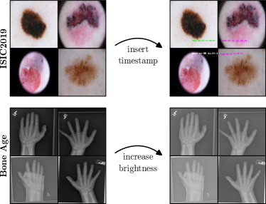
Figure 11: Examples from controlled datasets with clean (left) and attacked (right) samples for ISIC2019 (top) and Bone Age (bottom), with timestamp and brightness artifacts, respectively.

B.1.2 FunnyBirds Dataset

FunnyBirds [22] provides a framework to synthesize images of different classes of birds. Specifically, a bird is defined using 5 parts, for which the authors manually designed different types (4 beaks, 3 eyes, 4 feet, 9 tails, 6 wings). Further varying color, this leads to 2592 possible combinations, i.e., classes. We define a concept as a combination of part, type and color. For example, the concept “beak::beak-01::yellow” entails the beak shape beak-01 in color yellow. As outlined in Section 4.1 in the main paper, we construct a new version of FunnyBirds with 10 classes, with exactly one valid feature, i.e. concept, per class. While the class-defining concept is identical for all samples per class, all other concepts are chosen randomly per sample. The class-defining concepts are listed in Tab. 3. When training models on this dataset, the class-defining property must be used by the model. We synthesize 500 training samples and 100 test samples per class, totaling to 5000 training and 1000 test samples. The training set is further split into training/validation splits (90%/10%). In order to remove concepts, e.g., for the computation of sample-wise ground truth concept directions, we replace the class-defining property with another randomly chosen concept (e.g., “beak::beak-01::yellow” $\rightarrow$ “beak::beak-03::yellow”), while keeping other parts unchanged. Examples for original and manipulated samples are shown in Fig. 12.

Table 3: Class-defining concepts (part/shape/color) for all 10 classes in our synthetic FunnyBirds dataset.

	class-defining concept
class	part	shape	color
1	beak	beak-01	yellow
2	beak	beak-02	yellow
3	beak	beak-03	yellow
4	beak	beak-04	yellow
5	wing	wing-01	red
6	wing	wing-02	red
7	wing	wing-01	green
8	wing	wing-02	green
9	wing	wing-01	blue
10	wing	wing-02	blue

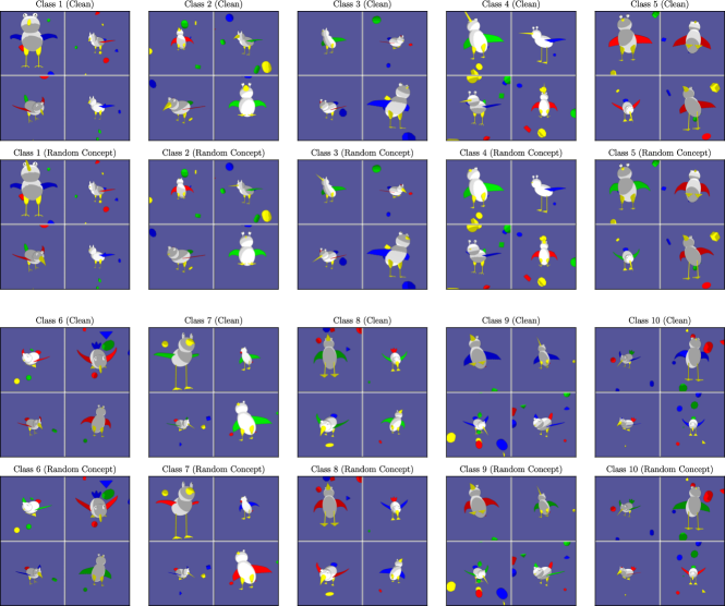
Figure 12: Examples for samples from all 10 classes from our synthetic FunnyBirds dataset, including clean samples (top) and identical samples with class-defining concept randomized (bottom).

B.2 Training Details

Tab. 4 provides training details for all models and datasets, including optimizer, learning rate (LR), number of epochs, and milestones, after which we divide the LR by 10. All models are pre-trained on ImageNet [14] with weights provided from the PyTorch model zoo.

Table 4: Model training details including optimizer, learning Rate (LR), number of epochs, and milestones, after which the learning rate is divided by 10.

				epochs
dataset	model	optimizer	LR	(milestones)
Bone Age	VGG16	SGD	0.05	100 (50,80)
	ResNet18	SGD	0.05	100 (50,80)
	EfficientNet-B0	Adam	0.01	100 (50,80)
ISIC2019 (controlled)	VGG16	SGD	0.05	150 (80,120)
	ResNet18	SGD	0.05	150 (80,120)
	EfficientNet-B0	Adam	0.01	150 (80,120)
ISIC2019 (real)	VGG16	SGD	0.05	150 (80,120)
	ResNet18	SGD	0.05	150 (80,120)
	EfficientNet-B0	Adam	0.01	150 (80,120)
Funny Birds	VGG16	SGD	0.01	50 (30)
	ResNet18	SGD	0.01	50 (30)
	EfficientNet-B0	Adam	0.01	50 (30)

Appendix C Additional Experimental Results

C.1 Detailed CAV Alignment Results

Additional CAV alignment results, including filter-(Lasso, Logistic, Ridge, and SVM) and pattern-CAVs are shown in Figs 13, 14, and 15 for ISIC2019, Figs 16, 17, and 18 for Pediatric Bone Age, and Figs 19, 20, and 21 for FunnyBirds, for VGG16, ResNet18, and EfficientNet-B0 models, respectively. The results confirm the trends described in the main paper in Section 4.2, i.e., a higher alignment with the ground truth concept direction for pattern-CAVs and a better concept separability for filter-CAVs.

Moreover, we report the cosine similarities between CAVs obtained with different feature pre-processing methods (centering, max-scaling, and their combination) and the ground truth concept direction for ISIC2019 and Bone Age datasets on the last Conv layers of ResNet18 and EfficientNet-B0 in Fig. 22 and Fig. 23, respectively.

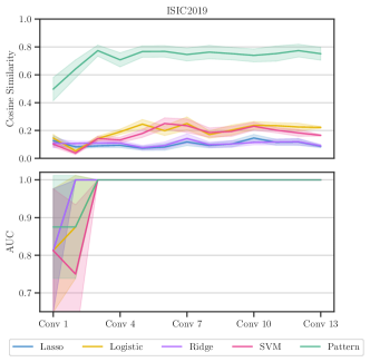
Figure 13: Comparison of cosine similarity between CAVs and true concept direction (top) and concept separability as AUC (bottom), using filter- (lasso, logistic, ridge, and SVM) and pattern-CAV, and for all Conv layers of VGG16 trained on ISIC2019.

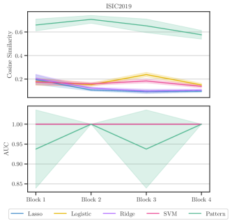
Figure 14: Comparison of cosine similarity between CAVs and true concept direction (top) and concept separability as AUC (bottom), using filter- (lasso, logistic, ridge, and SVM) and pattern-CAV, and after each block of ResNet18 trained on ISIC2019.

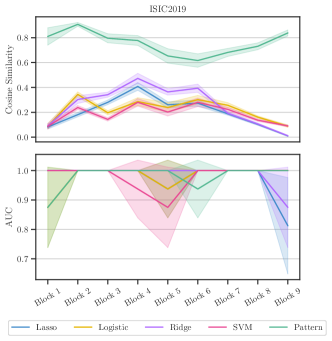
Figure 15: Comparison of cosine similarity between CAVs and true concept direction (top) and concept separability as AUC (bottom), using filter- (lasso, logistic, ridge, and SVM) and pattern-CAV, and after each block of EfficientNet-B0 trained on ISIC2019.

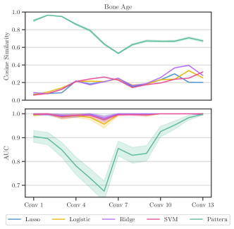
Figure 16: Comparison of cosine similarity between CAVs and true concept direction (top) and concept separability as AUC (bottom), using filter- (lasso, logistic, ridge, and SVM) and pattern-CAV, and after each Conv layer of VGG16 trained on the Pediatric Bone Age dataset.

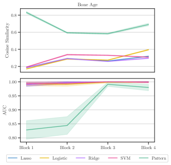
Figure 17: Comparison of cosine similarity between CAVs and true concept direction (top) and concept separability as AUC (bottom), using filter- (lasso, logistic, ridge, and SVM) and pattern-CAV, and after each block of ResNet18 trained on the Pediatric Bone Age dataset.

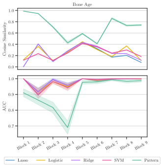
Figure 18: Comparison of cosine similarity between CAVs and true concept direction (top) and concept separability as AUC (bottom), using filter- (lasso, logistic, ridge, and SVM) and pattern-CAV, and after each block of EfficientNet-B0 trained on the Pediatric Bone Age dataset.

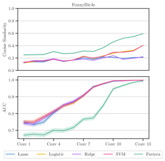
Figure 19: Comparison of cosine similarity between CAVs and true concept direction (top) and concept separability as AUC (bottom), using filter- (lasso, logistic, ridge, and SVM) and pattern-CAV, and after each Conv layer of VGG16 trained on FunnyBirds.

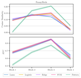
Figure 20: Comparison of cosine similarity between CAVs and true concept direction (top) and concept separability as AUC (bottom), using filter- (lasso, logistic, ridge, and SVM) and pattern-CAV, and after each block of ResNet18 trained on FunnyBirds.

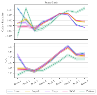
Figure 21: Comparison of cosine similarity between CAVs and true concept direction (top) and concept separability as AUC (bottom), using filter- (lasso, logistic, ridge, and SVM) and pattern-CAV, and after each block of EfficientNet-B0 trained on FunnyBirds.

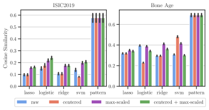
Figure 22: Cosine similarity between true concept direction $\mathbf{h}^{\text{gt}}$ and CAVs with different pre-processing methods fitted on the last Conv layer of ResNet18 trained on ISIC2019 (left) and Bone Age (right). Compared to filter-CAVs, pattern-CAV has a higher alignment with $\mathbf{h}^{\text{gt}}$ and is invariant to feature pre-processing.

Figure 23: Cosine similarity between true concept direction $\mathbf{h}^{\text{gt}}$ and CAVs with different pre-processing methods fitted on the last Conv layer of EfficientNet-B0 trained on ISIC2019 (left) and Bone Age (right). Compared to filter-CAVs, pattern-CAV has a higher alignment with $\mathbf{h}^{\text{gt}}$ and is invariant to feature pre-processing.

C.2 Qualitative CAV Results

Following-up on the qualitative approach on Section 4.2, we present further RelMax visualizations for the most important neurons for different CAVs in Fig 25. In contrast to Fig. 2 in the main paper, we include all our CAV approaches, namely 4 filter-based (lasso, logistic, ridge, and SVM) and the pattern-based CAV. Again, all filter-CAVs include unrelated neurons, whereas the pattern-CAV mainly includes neurons focusing on the concept of interest.

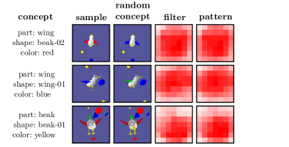
Figure 24: Visualization of concept sensitivity maps, measured as element-wise product $\boldsymbol{\nabla}_{\mathbf{a}}\tilde{f}(\mathbf{a}(\mathbf{a}))\odot\mathbf{h}$ using filter- (SVM) and pattern-CAVs for three concepts on the last Conv layer of ResNet18. All CAV variants detect a positive concept sensitivity (red) across all spatial locations ($7\times 7$ pixels). This makes ResNet18 less susceptible to noise.

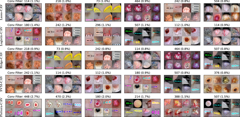
Figure 25: RelMax visualization for neurons corresponding to the largest absolute values in different CAVs, including 4 filter- (lasso, logistic, ridge, and SVM) and the pattern-CAVs, along with the Conv filter ID and the fraction of all (absolute) CAV values. While the filter-CAV picks up noisy neurons, the pattern-CAV uses neurons related to the relevant concept.

C.3 Qualitative TCAV Results

Extending on our qualitative TCAV results from Section 4.3.1, we show further sensitivity heatmaps for all considered CAV types, including four filter- (lasso, logistic, ridge, SVM) and our pattern-CAV in Fig. 26. We observe similar trends as in the main paper. Specifically, filter-CAVs lead to noisy sensitivity heatmaps, negatively impacting the TCAV score, while pattern-CAV precisely localizes the concept with positive sensitivity.

Note, that for ResNet18, instead of precisely localizing concepts, the sensitivity in the last Conv layer spreads over the entire sample ($7\times 7$ pixels), as shown in Fig. 24. Therefore, TCAV scores for ResNet18 are less impacted by noisy concept sensitivity maps in irrelevant regions.

Figure 26: Visualization of sensitivity maps, measured as element-wise product $\boldsymbol{\nabla}_{\mathbf{a}}\tilde{f}(\mathbf{a}(\mathbf{a}))\odot\mathbf{h}$ using different filter- (lasso, logistic, ridge, and SVM) and pattern-CAVs for three concepts with VGG16 (middle) and EfficientNet-B0 (right). Results are shown for the respective last Conv layer, upsampled to input space dimensions. While pattern-CAVs precisely localize the concepts, filter-CAVs lead to noisy sensitivity maps.

C.4 Model Correction with RR-ClArC

Model correction is performed with RR-ClArC for 10 epochs with the initial training learning rate (see Table 4) divided by 10. To balance between classification loss and the added loss term $L_{\text{RR}}$, we weigh the latter term with $\lambda\in\{10^{5},5\cdot 10^{5},10^{6},...,5\cdot 10^{9}\}$. The parameter is picked on the validation set and selected $\lambda$ values for all model correction experiments are shown in Tab. 5.

The results for our controlled datasets (Bone Age and ISIC2019) including standard errors are shown in Table 6. Moreover, Tab. 7 presents the model correction results for all artifacts (“band-aid”, “ruler”, and “skin marker”). Pattern-CAVs consistently yield better scores for artifact sensitivity, i.e., low artifact relevance and $\Delta\text{TCAV}^{\text{gt}}$ after model correction.

Fig. 27 presents additional relevance heatmaps after model correction w.r.t. the real ISIC2019 artifacts for all CAV variants and their difference heatmap compared with the Vanilla model.

Table 5: Selected $\lambda$ values for model correction with RR-ClArC as weight for the added loss term for experiments with VGG16, ResNet18, and EfficientNet-B0 with Bone Age (controlled), ISIC2019 (controlled), and ISIC2019 (real artifacts). For the latter, we run separate corrections w.r.t. the “band-aid” (BA), “ruler” (R), and “skin marker” (SM) artifacts.

		Bone Age	ISIC2019	ISIC2019
model	CAV	(controlled)	(controlled)	(BA$|$R$|$SM)
VGG16	Lasso	$10^{7}$	$10^{7}$	$5\cdot 10^{7}|1\cdot 10^{8}|1\cdot 10^{7}$
	Logistic	$5\cdot 10^{8}$	$10^{7}$	$5\cdot 10^{7}|1\cdot 10^{8}|1\cdot 10^{7}$
	Ridge	$5\cdot 10^{8}$	$10^{7}$	$5\cdot 10^{7}|1\cdot 10^{8}|1\cdot 10^{7}$
	SVM	$5\cdot 10^{7}$	$10^{7}$	$1\cdot 10^{7}|5\cdot 10^{7}|1\cdot 10^{7}$
	Pattern	$5\cdot 10^{8}$	$10^{7}$	$5\cdot 10^{7}|1\cdot 10^{9}|1\cdot 10^{7}$
ResNet18	Lasso	$5\cdot 10^{9}$	$10^{6}$	$1\cdot 10^{5}|5\cdot 10^{5}|5\cdot 10^{5}$
	Logistic	$5\cdot 10^{9}$	$5\cdot 10^{9}$	$1\cdot 10^{5}|5\cdot 10^{5}|5\cdot 10^{5}$
	Ridge	$10^{9}$	$5\cdot 10^{7}$	$1\cdot 10^{5}|1\cdot 10^{6}|5\cdot 10^{5}$
	SVM	$10^{8}$	$5\cdot 10^{9}$	$5\cdot 10^{5}|1\cdot 10^{5}|1\cdot 10^{5}$
	Pattern	$5\cdot 10^{9}$	$5\cdot 10^{9}$	$1\cdot 10^{5}|1\cdot 10^{6}|5\cdot 10^{5}$
Efficient Net-B0	Lasso	$10^{9}$	$10^{6}$	$5\cdot 10^{6}|1\cdot 10^{6}|5\cdot 10^{5}$
	Logistic	$5\cdot 10^{9}$	$10^{6}$	$5\cdot 10^{5}|1\cdot 10^{5}|5\cdot 10^{5}$
	Ridge	$5\cdot 10^{9}$	$10^{6}$	$1\cdot 10^{6}|5\cdot 10^{5}|1\cdot 10^{5}$
	SVM	$5\cdot 10^{9}$	$10^{7}$	$1\cdot 10^{5}|1\cdot 10^{5}|1\cdot 10^{5}$
	Pattern	$5\cdot 10^{8}$	$10^{6}$	$1\cdot 10^{6}|5\cdot 10^{5}|1\cdot 10^{5}$

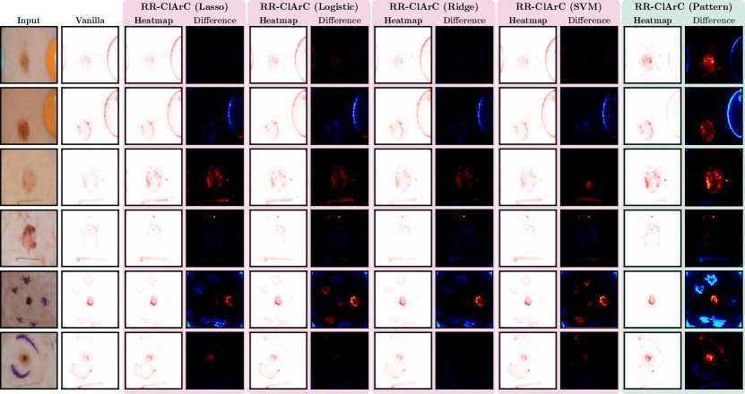
Figure 27: Additional qualitative results for model correction w.r.t. real artifacts band-aid (top two), ruler (middle two), and skin marker (bottom two) in ISIC2019 using VGG16. In addition to attribution heatmaps for models corrected with filter- (lasso, logistic, ridge, and SVM) and pattern-CAVs, we show heatmaps highlighting the differences compared to the Vanilla model attribution heatmap, with red and blue indicating higher and lower relevance after correction, respectively. Whereas filte-CAVs have limited impact, pattern-CAVs successfully increases the relevance on the mole and decreased the relevance on data artifacts.

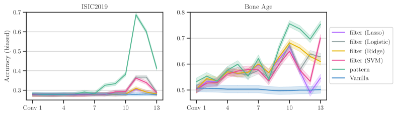
Figure 28: Accuracy on the biased test set for VGG16 trained on ISIC2019 (left) and Bone Age (right) and corrected with RR-ClArC with different CAV variants, including filter-based (lasso, logistic, ridge, and SVM) and pattern-based, fitted on each Conv layer. Confirming our observations from Fig. 8, pattern-CAV consistently outperforms filter-based CAVs on layers closer to the model output.

Table 6: Results after model correction with RR-ClArC for VGG16, ResNet18, and EfficientNet-B0 trained on Bone Age $|$ ISIC2019 (controlled) including standard errors. We report accuracy on clean and biased test set, the fraction of relevance put onto the data artifact region for localizable artifacts, and the TCAV score (reported as $\Delta\text{TCAV}^{\text{gt}}$) using the sample-wise ground-truth concept direction $\mathbf{h}^{\text{gt}}$, measuring the models’ sensitivity towards the artifacts after model correction. Arrows indicate whether low ($\downarrow$) or high ($\uparrow$) are better.

model	CAV	Accuracy (clean) $\uparrow$	Accuracy (biased) $\uparrow$	Artifact relevance $\downarrow$	$\Delta\text{TCAV}^{\text{gt}}$ $\downarrow$
VGG-16	Vanilla	${0.78\pm 0.01}$ $\,|\,$ ${0.82\pm 0.01}$	${0.50\pm 0.01}$ $\,|\,$ ${0.28\pm 0.01}$	- $\,|\,$ ${0.62\pm 0.01}$	${0.29\pm 0.00}$ $\,|\,$ ${0.14\pm 0.02}$
	lasso	${0.77\pm 0.01}$ $\,|\,$ ${0.82\pm 0.01}$	${0.55\pm 0.01}$ $\,|\,$ ${0.30\pm 0.01}$	- $\,|\,$ ${0.60\pm 0.01}$	${0.25\pm 0.00}$ $\,|\,$ ${0.13\pm 0.02}$
	logistic	${0.72\pm 0.01}$ $\,|\,$ ${0.82\pm 0.01}$	${0.63\pm 0.01}$ $\,|\,$ ${0.37\pm 0.01}$	- $\,|\,$ ${0.54\pm 0.01}$	${0.25\pm 0.00}$ $\,|\,$ $\mathbf{0.07\pm 0.02}$
	ridge	${0.71\pm 0.01}$ $\,|\,$ ${0.82\pm 0.01}$	${0.61\pm 0.01}$ $\,|\,$ ${0.31\pm 0.01}$	- $\,|\,$ ${0.59\pm 0.01}$	${0.24\pm 0.00}$ $\,|\,$ ${0.13\pm 0.02}$
	SVM	${0.69\pm 0.01}$ $\,|\,$ ${0.81\pm 0.01}$	${0.70\pm 0.01}$ $\,|\,$ ${0.36\pm 0.01}$	- $\,|\,$ ${0.55\pm 0.01}$	${0.24\pm 0.00}$ $\,|\,$ ${0.10\pm 0.02}$
	Pattern (ours)	${0.78\pm 0.01}$ $\,|\,$ ${0.80\pm 0.01}$	$\mathbf{0.75\pm 0.01}$ $\,|\,$ $\mathbf{0.69\pm 0.01}$	- $\,|\,$ $\mathbf{0.26\pm 0.01}$	$\mathbf{0.14\pm 0.00}$ $\,|\,$ ${0.10\pm 0.02}$
ResNet-18	Vanilla	${0.76\pm 0.01}$ $\,|\,$ ${0.84\pm 0.01}$	${0.48\pm 0.01}$ $\,|\,$ ${0.54\pm 0.01}$	- $\,|\,$ ${0.30\pm 0.01}$	${0.50\pm 0.00}$ $\,|\,$ ${0.50\pm 0.00}$
	lasso	${0.75\pm 0.01}$ $\,|\,$ ${0.84\pm 0.01}$	${0.69\pm 0.01}$ $\,|\,$ ${0.54\pm 0.01}$	- $\,|\,$ ${0.29\pm 0.01}$	${0.50\pm 0.00}$ $\,|\,$ ${0.50\pm 0.00}$
	logistic	${0.73\pm 0.01}$ $\,|\,$ ${0.83\pm 0.01}$	$\mathbf{0.74\pm 0.01}$ $\,|\,$ ${0.60\pm 0.01}$	- $\,|\,$ ${0.29\pm 0.01}$	${0.49\pm 0.00}$ $\,|\,$ $\mathbf{0.49\pm 0.01}$
	ridge	${0.77\pm 0.01}$ $\,|\,$ ${0.83\pm 0.01}$	${0.67\pm 0.01}$ $\,|\,$ ${0.55\pm 0.01}$	- $\,|\,$ ${0.29\pm 0.01}$	${0.50\pm 0.00}$ $\,|\,$ ${0.50\pm 0.00}$
	SVM	${0.74\pm 0.01}$ $\,|\,$ ${0.82\pm 0.01}$	${0.73\pm 0.01}$ $\,|\,$ ${0.59\pm 0.01}$	- $\,|\,$ ${0.29\pm 0.01}$	${0.50\pm 0.00}$ $\,|\,$ $\mathbf{0.49\pm 0.01}$
	Pattern (ours)	${0.75\pm 0.01}$ $\,|\,$ ${0.76\pm 0.01}$	${0.67\pm 0.01}$ $\,|\,$ $\mathbf{0.73\pm 0.01}$	- $\,|\,$ $\mathbf{0.28\pm 0.01}$	$\mathbf{0.48\pm 0.00}$ $\,|\,$ $\mathbf{0.49\pm 0.01}$
Efficient Net-B0	Vanilla	${0.79\pm 0.01}$ $\,|\,$ ${0.87\pm 0.01}$	${0.46\pm 0.01}$ $\,|\,$ ${0.55\pm 0.01}$	- $\,|\,$ ${0.55\pm 0.01}$	${0.46\pm 0.00}$ $\,|\,$ ${0.39\pm 0.02}$
	lasso	${0.79\pm 0.01}$ $\,|\,$ ${0.87\pm 0.01}$	${0.47\pm 0.01}$ $\,|\,$ ${0.55\pm 0.01}$	- $\,|\,$ ${0.55\pm 0.01}$	${0.45\pm 0.00}$ $\,|\,$ ${0.39\pm 0.02}$
	logistic	${0.79\pm 0.01}$ $\,|\,$ ${0.86\pm 0.01}$	${0.48\pm 0.01}$ $\,|\,$ ${0.54\pm 0.01}$	- $\,|\,$ ${0.55\pm 0.01}$	${0.44\pm 0.00}$ $\,|\,$ ${0.39\pm 0.02}$
	ridge	${0.79\pm 0.01}$ $\,|\,$ ${0.87\pm 0.01}$	${0.49\pm 0.01}$ $\,|\,$ ${0.55\pm 0.01}$	- $\,|\,$ ${0.55\pm 0.01}$	${0.44\pm 0.00}$ $\,|\,$ ${0.39\pm 0.02}$
	SVM	${0.79\pm 0.01}$ $\,|\,$ ${0.86\pm 0.01}$	${0.50\pm 0.01}$ $\,|\,$ ${0.54\pm 0.01}$	- $\,|\,$ ${0.55\pm 0.01}$	${0.44\pm 0.00}$ $\,|\,$ ${0.40\pm 0.02}$
	Pattern (ours)	${0.74\pm 0.01}$ $\,|\,$ ${0.86\pm 0.01}$	$\mathbf{0.61\pm 0.01}$ $\,|\,$ $\mathbf{0.61\pm 0.01}$	- $\,|\,$ $\mathbf{0.52\pm 0.01}$	$\mathbf{0.37\pm 0.01}$ $\,|\,$ $\mathbf{0.38\pm 0.02}$

Table 7: Results for VGG16, ResNet18, and EfficientNet-B0 trained on ISIC2019 after model correction with RR-ClArC w.r.t. to the real artifacts “band-aid”$|$“ruler”$|$“skin marker”. We report accuracy on clean and biased test set, the fraction of relevance put onto the data artifact region for localizable artifacts, and the TCAV score (reported as $\Delta\text{TCAV}^{\text{gt}}$) using the sample-wise ground-truth concept direction $\mathbf{h}^{\text{gt}}$, measuring the models’ sensitivity towards the artifacts after model correction. Note, that we artificially insert artifacts using estimated localization masks to create a biased test set and to compute $\mathbf{h}^{\text{gt}}$. Arrows indicate whether low ($\downarrow$) or high ($\uparrow$) are better.

model	CAV	Accuracy (clean) $\uparrow$	Accuracy (biased) $\uparrow$	Artifact relevance $\downarrow$	$\Delta\text{TCAV}^{\text{gt}}$ $\downarrow$
VGG-16	Vanilla	${0.83}$ $\,|\,$ ${0.83}$ $\,|\,$ ${0.83}$	${0.75}$ $\,|\,$ ${0.72}$ $\,|\,$ ${0.75}$	${0.51}$ $\,|\,$ ${0.32}$ $\,|\,$ ${0.23}$	${0.10}$ $\,|\,$ ${0.07}$ $\,|\,$ ${0.04}$
	lasso	${0.81}$ $\,|\,$ ${0.82}$ $\,|\,$ ${0.82}$	${0.77}$ $\,|\,$ ${0.77}$ $\,|\,$ $\mathbf{0.75}$	${0.48}$ $\,|\,$ ${0.25}$ $\,|\,$ ${0.22}$	${0.12}$ $\,|\,$ ${0.07}$ $\,|\,$ $\mathbf{0.05}$
	logistic	${0.82}$ $\,|\,$ ${0.81}$ $\,|\,$ ${0.81}$	${0.78}$ $\,|\,$ ${0.75}$ $\,|\,$ $\mathbf{0.75}$	${0.46}$ $\,|\,$ ${0.28}$ $\,|\,$ ${0.22}$	${0.09}$ $\,|\,$ ${0.07}$ $\,|\,$ $\mathbf{0.05}$
	ridge	${0.81}$ $\,|\,$ ${0.82}$ $\,|\,$ ${0.82}$	${0.76}$ $\,|\,$ ${0.77}$ $\,|\,$ $\mathbf{0.75}$	${0.49}$ $\,|\,$ ${0.26}$ $\,|\,$ ${0.22}$	${0.12}$ $\,|\,$ ${0.07}$ $\,|\,$ $\mathbf{0.05}$
	SVM	${0.82}$ $\,|\,$ ${0.82}$ $\,|\,$ ${0.81}$	${0.78}$ $\,|\,$ ${0.74}$ $\,|\,$ $\mathbf{0.75}$	${0.46}$ $\,|\,$ ${0.28}$ $\,|\,$ ${0.22}$	${0.11}$ $\,|\,$ ${0.07}$ $\,|\,$ $\mathbf{0.05}$
	Pattern (ours)	${0.82}$ $\,|\,$ ${0.82}$ $\,|\,$ ${0.82}$	$\mathbf{0.79}$ $\,|\,$ $\mathbf{0.79}$ $\,|\,$ $\mathbf{0.75}$	$\mathbf{0.31}$ $\,|\,$ $\mathbf{0.18}$ $\,|\,$ $\mathbf{0.18}$	$\mathbf{0.03}$ $\,|\,$ $\mathbf{0.06}$ $\,|\,$ $\mathbf{0.05}$
ResNet-18	Vanilla	${0.84}$ $\,|\,$ ${0.84}$ $\,|\,$ ${0.84}$	${0.79}$ $\,|\,$ ${0.80}$ $\,|\,$ ${0.78}$	${0.26}$ $\,|\,$ ${0.15}$ $\,|\,$ ${0.15}$	${0.47}$ $\,|\,$ ${0.45}$ $\,|\,$ ${0.39}$
	lasso	${0.84}$ $\,|\,$ ${0.84}$ $\,|\,$ ${0.84}$	$\mathbf{0.79}$ $\,|\,$ ${0.80}$ $\,|\,$ $\mathbf{0.78}$	$\mathbf{0.26}$ $\,|\,$ ${0.15}$ $\,|\,$ $\mathbf{0.15}$	${0.47}$ $\,|\,$ ${0.44}$ $\,|\,$ ${0.39}$
	logistic	${0.84}$ $\,|\,$ ${0.84}$ $\,|\,$ ${0.84}$	$\mathbf{0.79}$ $\,|\,$ ${0.80}$ $\,|\,$ $\mathbf{0.78}$	$\mathbf{0.26}$ $\,|\,$ ${0.15}$ $\,|\,$ $\mathbf{0.15}$	$\mathbf{0.46}$ $\,|\,$ ${0.45}$ $\,|\,$ ${0.39}$
	ridge	${0.84}$ $\,|\,$ ${0.84}$ $\,|\,$ ${0.84}$	$\mathbf{0.79}$ $\,|\,$ $\mathbf{0.81}$ $\,|\,$ $\mathbf{0.78}$	$\mathbf{0.26}$ $\,|\,$ ${0.15}$ $\,|\,$ $\mathbf{0.15}$	${0.47}$ $\,|\,$ ${0.43}$ $\,|\,$ ${0.39}$
	SVM	${0.84}$ $\,|\,$ ${0.84}$ $\,|\,$ ${0.84}$	$\mathbf{0.79}$ $\,|\,$ ${0.80}$ $\,|\,$ $\mathbf{0.78}$	$\mathbf{0.26}$ $\,|\,$ ${0.15}$ $\,|\,$ $\mathbf{0.15}$	${0.47}$ $\,|\,$ ${0.45}$ $\,|\,$ ${0.39}$
	Pattern (ours)	${0.83}$ $\,|\,$ ${0.83}$ $\,|\,$ ${0.83}$	$\mathbf{0.79}$ $\,|\,$ $\mathbf{0.81}$ $\,|\,$ ${0.77}$	$\mathbf{0.26}$ $\,|\,$ $\mathbf{0.13}$ $\,|\,$ ${0.16}$	$\mathbf{0.46}$ $\,|\,$ $\mathbf{0.35}$ $\,|\,$ $\mathbf{0.30}$
Efficient Net-B0	Vanilla	${0.87}$ $\,|\,$ ${0.87}$ $\,|\,$ ${0.87}$	${0.82}$ $\,|\,$ ${0.85}$ $\,|\,$ ${0.82}$	${0.37}$ $\,|\,$ ${0.11}$ $\,|\,$ ${0.23}$	${0.20}$ $\,|\,$ ${0.11}$ $\,|\,$ ${0.09}$
	lasso	${0.87}$ $\,|\,$ ${0.87}$ $\,|\,$ ${0.87}$	$\mathbf{0.82}$ $\,|\,$ $\mathbf{0.85}$ $\,|\,$ $\mathbf{0.82}$	${0.37}$ $\,|\,$ $\mathbf{0.11}$ $\,|\,$ $\mathbf{0.23}$	${0.19}$ $\,|\,$ ${0.11}$ $\,|\,$ ${0.09}$
	logistic	${0.87}$ $\,|\,$ ${0.87}$ $\,|\,$ ${0.87}$	$\mathbf{0.82}$ $\,|\,$ $\mathbf{0.85}$ $\,|\,$ $\mathbf{0.82}$	${0.37}$ $\,|\,$ $\mathbf{0.11}$ $\,|\,$ $\mathbf{0.23}$	${0.18}$ $\,|\,$ ${0.12}$ $\,|\,$ $\mathbf{0.08}$
	ridge	${0.87}$ $\,|\,$ ${0.87}$ $\,|\,$ ${0.87}$	$\mathbf{0.82}$ $\,|\,$ $\mathbf{0.85}$ $\,|\,$ $\mathbf{0.82}$	${0.37}$ $\,|\,$ $\mathbf{0.11}$ $\,|\,$ $\mathbf{0.23}$	${0.19}$ $\,|\,$ ${0.11}$ $\,|\,$ $\mathbf{0.08}$
	SVM	${0.87}$ $\,|\,$ ${0.87}$ $\,|\,$ ${0.87}$	$\mathbf{0.82}$ $\,|\,$ $\mathbf{0.85}$ $\,|\,$ $\mathbf{0.82}$	${0.37}$ $\,|\,$ $\mathbf{0.11}$ $\,|\,$ $\mathbf{0.23}$	${0.19}$ $\,|\,$ ${0.11}$ $\,|\,$ $\mathbf{0.08}$
	Pattern (ours)	${0.84}$ $\,|\,$ ${0.86}$ $\,|\,$ ${0.86}$	${0.79}$ $\,|\,$ $\mathbf{0.85}$ $\,|\,$ ${0.81}$	$\mathbf{0.34}$ $\,|\,$ $\mathbf{0.11}$ $\,|\,$ $\mathbf{0.23}$	$\mathbf{0.14}$ $\,|\,$ $\mathbf{0.10}$ $\,|\,$ $\mathbf{0.08}$

References

- [1] Reduan Achtibat, Maximilian Dreyer, Ilona Eisenbraun, Sebastian Bosse, Thomas Wiegand, Wojciech Samek, and Sebastian Lapuschkin. From attribution maps to human-understandable explanations through concept relevance propagation. Nature Machine Intelligence, 5(9):1006–1019, 2023.
- [2] Guillaume Alain and Yoshua Bengio. Understanding intermediate layers using linear classifier probes. International Conference on Learning Representations, 2017.
- [3] Christopher J. Anders, David Neumann, Wojciech Samek, Klaus-Robert Müller, and Sebastian Lapuschkin. Software for dataset-wide xai: From local explanations to global insights with Zennit, CoRelAy, and ViRelAy, 2021.
- [4] Christopher J Anders, Leander Weber, David Neumann, Wojciech Samek, Klaus-Robert Müller, and Sebastian Lapuschkin. Finding and removing clever hans: Using explanation methods to debug and improve deep models. Information Fusion, 77:261–295, 2022.
- [5] Sebastian Bach, Alexander Binder, Grégoire Montavon, Frederick Klauschen, Klaus-Robert Müller, and Wojciech Samek. On pixel-wise explanations for non-linear classifier decisions by layer-wise relevance propagation. PloS one, 10(7):e0130140, 2015.
- [6] David Bau, Jun-Yan Zhu, Hendrik Strobelt, Agata Lapedriza, Bolei Zhou, and Antonio Torralba. Understanding the role of individual units in a deep neural network. Proceedings of the National Academy of Sciences, 117(48):30071–30078, 2020.
- [7] Titus J Brinker, Achim Hekler, Alexander H Enk, Joachim Klode, Axel Hauschild, Carola Berking, Bastian Schilling, Sebastian Haferkamp, Dirk Schadendorf, Tim Holland-Letz, et al. Deep learning outperformed 136 of 157 dermatologists in a head-to-head dermoscopic melanoma image classification task. European Journal of Cancer, 113:47–54, 2019.
- [8] Zhi Chen, Yijie Bei, and Cynthia Rudin. Concept whitening for interpretable image recognition. Nature Machine Intelligence, 2(12):772–782, 2020.
- [9] Noel CF Codella, David Gutman, M Emre Celebi, Brian Helba, Michael A Marchetti, Stephen W Dusza, Aadi Kalloo, Konstantinos Liopyris, Nabin Mishra, Harald Kittler, et al. Skin lesion analysis toward melanoma detection: A challenge at the 2017 international symposium on biomedical imaging (isbi), hosted by the international skin imaging collaboration (isic). In 15th International Symposium on Biomedical Imaging (ISBI 2018), pages 168–172. IEEE, 2018.
- [10] Marc Combalia, Noel CF Codella, Veronica Rotemberg, Brian Helba, Veronica Vilaplana, Ofer Reiter, Cristina Carrera, Alicia Barreiro, Allan C Halpern, Susana Puig, et al. Bcn20000: Dermoscopic lesions in the wild, 2019.
- [11] Corinna Cortes and Mehryar Mohri. Confidence intervals for the area under the roc curve. Advances in neural information processing systems, 17, 2004.
- [12] Corinna Cortes and Vladimir Vapnik. Support-vector networks. Machine learning, 20:273–297, 1995.
- [13] Jonathan Crabbé and Mihaela van der Schaar. Concept activation regions: A generalized framework for concept-based explanations. Advances in Neural Information Processing Systems, 35:2590–2607, 2022.
- [14] Jia Deng, Wei Dong, Richard Socher, Li-Jia Li, Kai Li, and Li Fei-Fei. Imagenet: A large-scale hierarchical image database. In IEEE conference on computer vision and pattern recognition, pages 248–255. IEEE, 2009.
- [15] Maximilian Dreyer, Frederik Pahde, Christopher J Anders, Wojciech Samek, and Sebastian Lapuschkin. From hope to safety: Unlearning biases of deep models by enforcing the right reasons in latent space. arXiv preprint arXiv:2308.09437, 2023.
- [16] Nelson Elhage, Tristan Hume, Catherine Olsson, Nicholas Schiefer, Tom Henighan, Shauna Kravec, Zac Hatfield-Dodds, Robert Lasenby, Dawn Drain, Carol Chen, et al. Toy models of superposition. arXiv preprint arXiv:2209.10652, 2022.
- [17] Thomas Fel, Agustin Picard, Louis Bethune, Thibaut Boissin, David Vigouroux, Julien Colin, Rémi Cadène, and Thomas Serre. Craft: Concept recursive activation factorization for explainability. In Proceedings of the IEEE/CVF Conference on Computer Vision and Pattern Recognition, pages 2711–2721, 2023.
- [18] Amirata Ghorbani, James Wexler, James Y Zou, and Been Kim. Towards automatic concept-based explanations. Advances in neural information processing systems, 32, 2019.
- [19] Safwan S Halabi, Luciano M Prevedello, Jayashree Kalpathy-Cramer, Artem B Mamonov, Alexander Bilbily, Mark Cicero, Ian Pan, Lucas Araújo Pereira, Rafael Teixeira Sousa, Nitamar Abdala, et al. The rsna pediatric bone age machine learning challenge. Radiology, 290(2):498–503, 2019.
- [20] Stefan Haufe, Frank Meinecke, Kai Görgen, Sven Dähne, John-Dylan Haynes, Benjamin Blankertz, and Felix Bießmann. On the interpretation of weight vectors of linear models in multivariate neuroimaging. Neuroimage, 87:96–110, 2014.
- [21] Kaiming He, Xiangyu Zhang, Shaoqing Ren, and Jian Sun. Deep residual learning for image recognition. In Proceedings of the IEEE Conference on Computer Vision and Pattern Recognition, pages 770–778, 2016.
- [22] Robin Hesse, Simone Schaub-Meyer, and Stefan Roth. Funnybirds: A synthetic vision dataset for a part-based analysis of explainable ai methods. In Proceedings of the IEEE/CVF International Conference on Computer Vision, pages 3981–3991, 2023.
- [23] Arthur E Hoerl and Robert W Kennard. Ridge regression: Biased estimation for nonorthogonal problems. Technometrics, 12(1):55–67, 1970.
- [24] Been Kim, Martin Wattenberg, Justin Gilmer, Carrie Cai, James Wexler, Fernanda Viegas, et al. Interpretability beyond feature attribution: Quantitative testing with concept activation vectors (tcav). In International Conference on Machine Learning, pages 2668–2677. PMLR, 2018.
- [25] Pieter Jan Kindermans, Kristof T Schütt, Maximilian Alber, Klaus-Robert Müller, Dumitru Erhan, Been Kim, and Sven Dähne. Learning how to explain neural networks: Patternnet and patternattribution. In Proceedings of the 6th International Conference on Learning Representations, ICLR 2018, 2018.
- [26] Maximilian Kohlbrenner, Alexander Bauer, Shinichi Nakajima, Alexander Binder, Wojciech Samek, and Sebastian Lapuschkin. Towards best practice in explaining neural network decisions with lrp. In 2020 International Joint Conference on Neural Networks (IJCNN), pages 1–7. IEEE, 2020.
- [27] Thomas McGrath, Andrei Kapishnikov, Nenad Tomašev, Adam Pearce, Martin Wattenberg, Demis Hassabis, Been Kim, Ulrich Paquet, and Vladimir Kramnik. Acquisition of chess knowledge in alphazero. Proceedings of the National Academy of Sciences, 119(47):e2206625119, 2022.
- [28] Neel Nanda, Andrew Lee, and Martin Wattenberg. Emergent linear representations in world models of self-supervised sequence models. In Proceedings of the 6th BlackboxNLP Workshop: Analyzing and Interpreting Neural Networks for NLP, pages 16–30, 2023.
- [29] Chris Olah, Alexander Mordvintsev, and Ludwig Schubert. Feature visualization. Distill, 2(11):e7, 2017.
- [30] Frederik Pahde, Maximilian Dreyer, Wojciech Samek, and Sebastian Lapuschkin. Reveal to revise: An explainable ai life cycle for iterative bias correction of deep models. In Medical Image Computing and Computer Assisted Intervention, 2023.
- [31] Jacob Pfau, Albert T Young, Jerome Wei, Maria L Wei, and Michael J Keiser. Robust semantic interpretability: Revisiting concept activation vectors, 2021.
- [32] Konpat Preechakul, Nattanat Chatthee, Suttisak Wizadwongsa, and Supasorn Suwajanakorn. Diffusion autoencoders: Toward a meaningful and decodable representation. In CVPR, pages 10619–10629, 2022.
- [33] Alec Radford, Rafal Jozefowicz, and Ilya Sutskever. Learning to generate reviews and discovering sentiment. arXiv preprint arXiv:1704.01444, 2017.
- [34] Nusrat Rouf, Majid Bashir Malik, Tasleem Arif, Sparsh Sharma, Saurabh Singh, Satyabrata Aich, and Hee-Cheol Kim. Stock market prediction using machine learning techniques: a decade survey on methodologies, recent developments, and future directions. Electronics, 10(21):2717, 2021.
- [35] Karen Simonyan and Andrew Zisserman. Very deep convolutional networks for large-scale image recognition. In Yoshua Bengio and Yann LeCun, editors, ICLR 2015, 2015.
- [36] Mingxing Tan and Quoc Le. Efficientnet: Rethinking model scaling for convolutional neural networks. In ICML, pages 6105–6114. PMLR, 2019.
- [37] Robert Tibshirani. Regression shrinkage and selection via the lasso. Journal of the Royal Statistical Society Series B: Statistical Methodology, 58(1):267–288, 1996.
- [38] Guido Vittorio Travaini, Federico Pacchioni, Silvia Bellumore, Marta Bosia, and Francesco De Micco. Machine learning and criminal justice: A systematic review of advanced methodology for recidivism risk prediction. International journal of environmental research and public health, 19(17):10594, 2022.
- [39] Philipp Tschandl, Cliff Rosendahl, and Harald Kittler. The ham10000 dataset, a large collection of multi-source dermatoscopic images of common pigmented skin lesions. Scientific data, 5(1):1–9, 2018.
- [40] Johanna Vielhaben, Stefan Bluecher, and Nils Strodthoff. Multi-dimensional concept discovery (mcd): A unifying framework with completeness guarantees. Transactions on Machine Learning Research, 2023.
- [41] Zihao Wang, Lin Gui, Jeffrey Negrea, and Victor Veitch. Concept algebra for (score-based) text-controlled generative models. In NeurIPS, 2023.
- [42] Mert Yuksekgonul, Maggie Wang, and James Zou. Post-hoc concept bottleneck models. In The Eleventh International Conference on Learning Representations, 2023.
- [43] Aleš Završnik. Algorithmic justice: Algorithms and big data in criminal justice settings. European Journal of criminology, 18(5):623–642, 2021.