Nonlinear structural stability and linear dynamic instability of transonic steady-states to a hydrodynamic model for semiconductors

¹College of Mathematics, Faculty of Science, Beijing University of Technology, Beijing 100022, China
²Department of Mathematics, Champlain College Saint-Lambert, Quebec, J4P 3P2, Canada
³Department of Mathematics and Statistics, McGill University, Montreal, Quebec, H3A 2K6, Canada
⁴School of Mathematics and Statistics, Northeast Normal University, Changchun 130024, China
Email : fyh@bjut.edu.cn,   ming.mei@mcgill.ca,    zhanggj100@nenu.edu.cn

Abstract. For unipolar hydrodynamic model of semiconductor device represented by Euler-Poisson equations, when the doping profile is supersonic, the existence of steady transonic shock solutions and $C^{\infty}$-smooth steady transonic solutions for Euler-Poisson Equations were established in [27] and [41], respectively. In this paper we further study the nonlinear structural stability and the linear dynamic instability of these steady transonic solutions. When the $C^{1}$-smooth transonic steady-states pass through the sonic line, they produce singularities for the system, and cause some essential difficulty in the proof of structural stability. For any relaxation time: $0<\tau\leq+\infty$, by means of elaborate singularity analysis, we first investigate the structural stability of the $C^{1}$-smooth transonic steady-states, once the perturbations of the initial data and the doping profiles are small enough. Moreover, when the relaxation time is large enough $\tau\gg 1$, under the condition that the electric field is positive at the shock location, we prove that the transonic shock steady-states are structurally stable with respect to small perturbations of the supersonic doping profile. Furthermore, we show the linearly dynamic instability for these transonic shock steady-states provided that the electric field is suitable negative. The proofs for the structural stability results are based on singularity analysis, a monotonicity argument on the shock position and the downstream density, and the stability analysis of supersonic and subsonic solutions. The linear dynamic instability of the steady transonic shock for Euler-Poisson equations can be transformed to the ill-posedness of a free boundary problem for the Klein-Gordon equation. By using a nontrivial transformation and the shooting method, we prove that the linearized problem has a transonic shock solution with exponential growths. These results enrich and develop the existing studies.

Keywords: Hydrodynamic model of semiconductors, Euler-Poisson equations, $C^{1}$-smooth transonic solutions, transonic shock solutions, structural stability, linear dynamic instability.

AMS Subject Classification (2000) : 35R35, 35Q35, 76N10, 35J70

1. Introduction and main results

1.1. Modeling equations

This paper is concerned with the smooth/shock transonic solutions for the one-dimensional hydrodynamic model for semiconductors, which is presented as Euler-Poisson equations with relaxation effect

(1.1) $$\begin{cases}n_{t}+(nu)_{x}=0,\\ (nu)_{t}+\left(P(n)+nu^{2}\right)_{x}=nE-\displaystyle{\frac{nu}{\tau}},\\ E_{x}=n-b(x).\end{cases}$$

This model describes several physical flows including the propagation of electrons in submicron semiconductor devices [4, 7, 14, 24, 34] and plasmas [40] (hydrodynamic model), and the biological transport of ions for channel proteins [8]. In the hydrodynamic model of semiconductor devices or plasma, $n$, $u$, $P$ and $E$ represent the electron density, macroscopic particle velocity, pressure and the electric field, respectively. The function $b=b(x)>0$ is the doping profile standing the impurity for the device. The parameter $\tau>0$ means the momentum relaxation time. While, the biological model describes the transport of ions between the extracellular side and the cytoplasmic side of membranes [8]. In this case, $n$, $nu$ and $E$ are the ion concentration, the ions translational mass, and the electric field, respectively, and the doping profile $b(x)$ represents a background density of charged ions.

For ideal gas law of isentropic case, the pressure function $P$ is physically represented by

$$P(n)=Tn^{\gamma},$$

where $T>0$ is a constant absolute temperature, and $\gamma>1$ represents the adiabatic exponent. In this article, we mainly consider the isothermal case, i.e., $\gamma=1$ for simplicity of analysis. The case of $\gamma>1$ can be similarly treated.

Using the terminology from gas dynamics, we call $c:=\sqrt{P^{\prime}(n)}=\sqrt{T}>0$ the sound speed for $P(n)=Tn$. Moreover, if we denote

(1.2) $$\begin{split}J:=nu,~{}~{}\mbox{ the current density of the flow, }\end{split}$$

and take $J>0$ without loss of generality, then the flow is supersonic/sonic/subsonic if the fluid velocity satisfies

(1.3) $${\rm fluid~{}~{}velocity}:u=\frac{J}{n}>({\rm or}~{}~{}=,~{}~{}{\rm or}~{}~{}<)~{}~{}c=\sqrt{P^{\prime}(n)}=\sqrt{T}:{\rm sound~{}~{}speed}.$$

Without loss of generality, we assume that $T=1$, i.e., $P(n)=n$. Thus, it can be identified that the flow is subsonic if $n>J$, sonic if $n=J$, and supersonic if $0<n<J$.

The main issue of the present paper is to study the structural stabilities for $C^{1}$-smooth transonic steady-states and transonic shock steady-states, and the linear dynamic instability for the transonic shock steady-states. These steady-states are solutions of the following time-independent equations

(1.4) $$\begin{cases}(nu)_{x}=0,\ i.e.,\ J=nu=\mbox{constant},\\ \left(n+nu^{2}\right)_{x}=nE-\displaystyle{\frac{nu}{\tau}},\\ E_{x}=n-b(x).\end{cases}$$

For convenience, we set

(1.5) $$\begin{split}\alpha:=\frac{1}{\tau},~{}~{}\mbox{ the reciprocal of the relaxation time of the current},\end{split}$$

thus system (1.4) is reduced to

(1.6) $$\begin{cases}\left(n+\displaystyle{\frac{J^{2}}{n}}\right)_{x}=nE-\alpha J,\\ E_{x}=n(x)-b(x),\end{cases}$$

equivalently,

(1.7) $$\begin{cases}\displaystyle{n_{x}=\frac{(nE-\alpha J)n^{2}}{n^{2}-J^{2}}=\frac{n^{2}E}{n+J}+\frac{Jn^{2}(E-\alpha)}{n^{2}-J^{2}},}\\ E_{x}=n-b.\end{cases}$$

Subjected to the stationary system (1.6) or its equivalent form (1.7), two different problems are proposed in this paper. One is the “initial value” problem for the system (1.7):

(1.8) $$\begin{cases}\displaystyle{n_{x}=\frac{n^{2}E}{n+J}+\frac{Jn^{2}(E-\alpha)}{n^{2}-J^{2}}},&x\in\mathbb{R}_{+},\\ E_{x}=n-b(x),&x\in\mathbb{R}_{+},\\ (n,E)|_{x=0}=(n_{0},E_{0}),\end{cases}$$

in which the initial data $n_{0}$ is considered to be supersonic satisfying

$$0<n_{0}<J$$

throughout the paper, because the case of the subsonic data $n_{0}>J$ can be similarly treated.

The other is the boundary value problem:

(1.9) $$\begin{cases}\displaystyle{\left(n+\frac{J^{2}}{n}\right)_{x}=nE-\alpha J},&0<x<L,\\ E_{x}=n-b(x),&0<x<L,\\ n(0)=n_{l},\ \ n(L)=n_{r},\end{cases}$$

where $L>0$, and the boundary conditions are considered to be

$$n_{l}<J<n_{r}$$

with the supersonic boundary value $n_{l}$ and the subsonic boundary value $n_{r}$ in the paper. The case of $n_{l}>J>n_{r}$ with the subsonic boundary value $n_{l}$ and the supersonic boundary value $n_{r}$ can be also similarly treated.

The boundary value problem (1.9), by dividing (1.9)₁ by $n$ and differentiating it with respect to $x$, is also equivalent to the following system,

(1.10) $$\begin{cases}\displaystyle{\Big{[}\Big{(}\frac{1}{n}-\frac{1}{n^{3}}\Big{)}n_{x}\Big{]}_{x}+\alpha\Big{(}\frac{J}{n}\Big{)}_{x}-[n-b(x)]=0,}&0<x<L\\ E_{x}=n-b(x),&0<x<L,\\ n(0)=n_{l},\ \ n(L)=n_{r}.\end{cases}$$

The $C^{1}$-smooth transonic solutions and the shock transonic solutions for the initial value problem of system (1.8) or the boundary value problem (1.9) are defined as follows, respectively.

Definition 1.1 ($C^{1}$-smooth transonic solutions).

A pair of $(n(x),E(x))$ with $n(x)>0$ is called a $C^{1}$-smooth transonic solution of the initial value problem (1.8), or the boundary value problem (1.9), if $(n,E)\in C^{1}(I)\times C^{2}(I)$ for $I:=\mathbb{R}_{+}$ or $I:=[0,L]$, and there exists a number $x_{0}>0$ such that

$$(n,E)=\left\{{\begin{array}[]{*{20}{c}}\vspace{3mm}{(n_{\rm sup},E_{\rm sup})(x),\hfill}&{{\rm as}\quad x\in[0,x_{0}],\hfill}\\ {(n_{\rm sub},E_{\rm sub})(x),\hfill}&{{\rm as}\quad x\geq x_{0},\hfill}\\ \end{array}}\right.$$

where $(n_{sup},E_{sup})(x)$ satisfying $0<n_{\rm sup}(x)<J$ on $(0,x_{0})$ is called to be supersonic, and $(n_{sub},E_{sub})(x)$ satisfying $n_{\rm sub}(x)>J$ for $x>x_{0}$ is subsonic, both of them are differentiable at the sonic line $n=J$:

(1.11) $$\begin{cases}n_{\rm sup}(x_{0})=n_{\rm sub}(x_{0})=J,\quad n^{\prime}_{\rm sup}(x_{0})=n^{\prime}_{\rm sub}(x_{0}),\\ E_{\rm sup}(x_{0})=E_{\rm sub}(x_{0}),\quad E^{\prime}_{\rm sup}(x_{0})=E^{\prime}_{\rm sub}(x_{0}).\quad E^{\prime\prime}_{\rm sup}(x_{0})=E^{\prime\prime}_{\rm sub}(x_{0}).\end{cases}$$

Definition 1.2 (Shock transonic solutions).

A pair of $(n(x),E(x))$ with $n(x)>0$ is called a transonic shock solution to problem (1.8) or (1.9), if there exists a point $x_{0}\in(0,L)$, such that

$$\left(n,E\right)=\left\{{\begin{array}[]{*{20}{c}}\vspace{3mm}{\left({{n_{\rm sup}},{E_{\rm sup}}}\right)(x),\hfill}&{{\rm as}\quad x\in[0,x_{0}),\hfill}\\ {\left({{n_{\rm sub}},{E_{\rm sub}}}\right)(x),\hfill}&{{\rm as}\quad x>x_{0},\hfill}\\ \end{array}}\right.$$

satisfies $0<n_{\rm sup}(x)<J$ on $(0,x_{0})$, $n_{\rm sub}(x)>J$ on $x>x_{0}$, and the entropy condition

(1.12) $$0<n_{\rm sup}(x_{0}^{-})<J<n_{\rm sub}(x_{0}^{+}),$$

and the Rankine-Hugoniot conditions

(1.13) $$n_{\rm sup}(x_{0}^{-})+\frac{J^{2}}{n_{\rm sup}(x_{0}^{-})}=n_{\rm sub}(x_{0}^{+})+\frac{J^{2}}{n_{\rm sub}(x_{0}^{+})},\quad E_{\rm sup}(x_{0}^{-})=E_{\rm sub}(x_{0}^{+}).$$

1.2. Background of research

Euler-Poisson equations have been an important topic in fluid dynamics and semiconductor device industry. One of interesting questions is to investigate their physical solutions such as subsonic/supersonic/transonic solutions. When the setting background of the steady-state system of Euler-Poisson equations is completely subsonic, namely, subsonic boundary and subsonic doping profile, Degond-Markowich [13] first established the existence of the subsonic solution, and proved its uniqueness once the steady-state system is strongly subsonic with $J\ll 1$. Since then, the steady subsonic flows were studied in great depth with different boundaries as well as the higher dimensions case in [3, 4, 13, 14, 15, 18, 23, 33, 36], see also the references therein. These subsonic steady-states with different settings are then extensively proved to be dynamically stable in [18, 25, 19, 20, 21, 35, 36] and the references there cited, once the initial perturbations around the subsonic steady-states are small enough.

Regarding the steady supersonic flows, the first result on the existence and uniqueness of the supersonic steady-states was obtained by Peng-Violet [38], when the doping profile and the boundary both are strongly supersonic. See also a recent study on supersonic steady-states for 3D potential flows [6], and the structural stability of 2-D supersonic steady-states elegantly proved by Bae-Duan-Xiao-Xie [5].

As we know, another interesting issue for Euler-Poisson equations is about the structure of transonic solutions. The first observation on such kind transonic shocks was made by Ascher-Markowich-Pietra-Schmeiser [1] when the boundary value problem (1.9) is with subsonic boundary data but a constant supersonic doping profile, which was then generalized by Rosini [39] for the non-isentropic flow. Furthermore, when the doping profile $b(x)$ is nonconstant, Gamba [16] constructed 1-D transonic solutions with shocks by the method of vanishing viscosity, then joint with Morawetz, they [17] showed the existence of transonic solutions with shocks in 2-D case. However, these solutions as the limits of vanishing viscosity yield some boundary layers. Hence, the question of well-posedness of the boundary value problem for the inviscid problem couldn’t be solved by the vanishing viscosity method. Late then, when Euler-Poisson equations are lack of the effect of the semiconductor (the case of $\tau=\infty$), Luo-Xin [32] and Luo-Rauch-Xie-Xin [31] studied the structure of transonic steady-states, and showed the existence/nonexistence and the uniqueness/nonuniqueness of the transonic solutions, once the stationary Euler-Poisson system possess a constant supersonic/subsonic doping profile, and one supersonic boundary and the other subsonic boundary. Some restrictions on the boundary and the domain are also needed. These transonic shocks with supersonic doping were proved to be structurally stable [31] when the doping profile is a small perturbation of the constant supersonic doping. Under certain restrictions, the time-asymptotic stability of the transonic shock profiles was also obtained in [31].

Recently, the study in this topic has made some profound progress [10, 11, 12, 26, 27, 41]. For Euler-Poisson equations with relaxation effect (1.1), when the boundary is subjected to be sonic (the critical case), Li-Mei-Zhang-Zhang [26, 27] first classified the structure of all type of physical solutions. That is, when the doping profile is subsonic, the steady Euler-Poisson system possesses a unique subsonic solution, at least one supersonic solution, and infinitely many shock transonic solutions if the semiconductor effect is weak ($\tau\gg 1$), and infinitely many $C^{1}$-smooth transonic solutions if the semiconductor effect is strong ($\tau\ll 1$); while, when the doping profile is supersonic and far from the sonic line, there is no any physical (subsonic/supersolic/transonic) solution. The supersonic solution and many shock-transonic solutions exist only when the doping profile is sufficiently close to the sonic line. Later, when the doping profile is transonic, according to two cases of the subsonic-dominated and supersonic-dominated doping profile, Chen-Mei-Zhang-Zhang [10] further classified the structure of all subsonic/supersonic/shock-transonic solutions. Very recently, by using the manifold analysis and singularity analysis near the sonic line and the singular point, Wei-Mei-Zhang-Zhang [41] further investigated the existence and regularity of the smooth transonic steady solutions of Euler-Poisson equations. They gave the detailed discussions on the structure of directions of the transonic solutions, and what kind regularity of the smooth transonic solutions. In particular, when the boundary states are separated in the supersonic regime and the subsonic regime, they obtained that the Euler-Poisson system with supersonic doping profile possesses two $C^{\infty}$-smooth transonic solutions, where one is from supersonic region to subsonic region and the other is of the inverse direction. Moreover, the existence of 2D and 3D radial subsonic/supersonic/transonic steady-states with the sonic boundary conditions were technically proved by Chen-Mei-Zhang-Zhang in [11] and [12], respectively.

Remarkably, when the system (1.9) is lack of the semiconductor effect, namely, the relaxation time $\tau=\infty$, i.e., $\alpha=0$, Luo-Rauch-Xie-Xin [31] artfully proved that, there exists a unique transonic shock for the system once the doping file is a supersonic constant $b=b_{0}<J$, and showed its structural stability, namely, there will exist another transonic shock solution for the doping profile $b(x)$ as a small perturbation of the supersonic doping $b_{0}$. Since the transonic shocks jump the sonic line from the supersonic regime to the subsonic regime, such that there is no singularity for the system (1.9) at the sonic line, namely, $n(x)\not=J$. This is an advantage for the proof of the structural stability of the transonic shocks, as we know.

However, for the smooth transonic solutions, they pass through the sonic line $n=J$, and make the system (1.7) to be singular at the sonic line (the denominator of (1.7) becomes zero, i.e., $n^{2}-J^{2}=0$). Different from the case of transonic shocks, this causes an essential difficulty to show the structural stability of the smooth transonic steady-states, and remains this problem to be open for any relaxation time $0<\tau\leq\infty$. To answer this question will be one of our main targets in the present paper. Here we have a key observation. By taking singularity analysis around the sonic line, we can heuristically determine the value of the derivative of the smooth transonic solution $n(x)$ at the singular point on the sonic line. This, with some exquisite singularity analysis together, can guarantee us to show the structural stability around the singular points, then to prove the structural stability of the smooth transonic steady-state for the initial value problem (1.8) (also the boundary value problem (1.9)) in the space $C^{1}_{loc}(\mathbb{R}_{+})\times C^{2}_{loc}(\mathbb{R}_{+})$ (or in the space $C^{1}[0,L]\times C^{2}[0,L]$). In fact, the carried-out analysis around the singular transition points on the sonic line is technical and challenging.

Moreover, when $\tau\gg 1$, we recognize that, the boundary value problem (1.7) and (1.9) possess the transonic shocks, once the doping profile is a supersonic constant, and these transonic shocks are also structurally stable, when the perturbed doping profile is small enough. Furthermore, we prove that these steady transonic shocks are dynamically unstable, when the electric field is negative. This part can be regarded as the generalizations of the previous study [31] with $\tau=\infty$ to the case of $\tau\gg 1$, but with some technical development.

1.3. Main results

In this subsection, we state our main results on the structural stabilities of smooth transonic steady-states and the transonic shock steady-states, respectively, and the linear dynamic instability of these transonic shock steady-states.

We first give the existence and uniqueness of $C^{1}$-smooth transonic steady-states and the transonic shock steady-states. This can be also seen from the following numerical simulations for the phase diagrams of $(n,E)$, for example, by taking $b(x)=0.5$, $J=1$, and $\tau=1$ in Figures 1 and 2. Here, there are two smooth curves cross the sonic line $n=J$, namely, two smooth transonic steady-states. One smooth transonic curve is from the supersonic regime to the subsonic regime (see Figure 1) by setting either the initial data $(n_{0},E_{0})$ to be supersonic $n_{0}<J$ or the boundary data to be $n_{l}<J<n_{r}$. The other smooth transonic curve is from the subsonic regime to the supersonic regime (see Figure 2) by setting either the initial data $(n_{0},E_{0})$ to be subsonic $n_{0}>J$ or the boundary data to be $n_{l}>J>n_{r}$.

In what follows, we mainly consider the case of transonic steady-states from the supersonic regime to the subsonic regime in Theorems 1.1-1.6. Of course, the results presented in Theorem 1.1-1.6 are also true for the case of transonic steady-states from the supersonic regime to the subsonic regime.

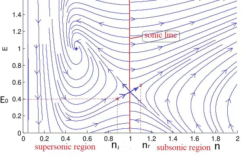
Figure 1. This is the $(n,E)$ portrait diagram by taking $b(x)=0.5$, $J=1$, and $\tau=1$. We mark one smooth curve (smooth transonic steady-state) passing through the sonic line $n=1$ from the supersonic regime to the subsonic regime.

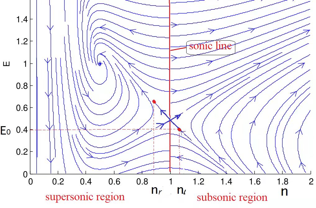
Figure 2. This is the $(n,E)$ portrait diagram by taking $b(x)=0.5$, $J=1$, and $\tau=1$. We mark the other smooth curve (smooth transonic steady-state) passing through the sonic line $n=1$ from the subsonic regime to the supersonic regime.

Theorem 1.1 (Existence and uniqueness of smooth/shock transonic steady-states).

Let the doping profile be supersonic such that $b(x)\in L^{\infty}(0,L)$ and $0<b(x)<J$.

• For any relaxation time $0<\tau\leq+\infty$, if $b(x)=b_{0}<J$ is a constant in the supersonic regime, then the stationary Euler-Poisson equations with the initial condition (1.8) (or the boundary value condition (1.9)) admit a unique $C^{1}$-smooth transonic solution $(n(x),E(x))$ passing through the sonic line $n(x)=J$ at a unique point $x_{0}>0$ determined implicitly from the system:

  $$(n,E)(x)=\begin{cases}(n_{sup},E_{sup})(x),&x\in[0,x_{0}]\\ (n_{sub},E_{sub})(x),&x\geq x_{0},\end{cases}$$

  and

  $$\begin{cases}n_{sup}(x_{0})=n_{sub}(x_{0})=J,\\ n^{\prime}_{sup}(x_{0})=n^{\prime}_{sub}(x_{0}),\\ E_{sup}(x_{0})=E_{sub}(x_{0})=\alpha=\frac{1}{\tau},\\ E^{\prime}_{sup}(x_{0})=E^{\prime}_{sub}(x_{0})=J-b_{0},\\ E^{\prime\prime}_{sup}(x_{0})=E^{\prime\prime}_{sub}(x_{0})=n_{x}(x_{0}).\end{cases}$$

  Here, for the initial value problem (1.8), the initial data $(n_{0},E_{0})$ is in the supersonic regime, satisfying $0<n_{0}<J$ and $E_{0}<\min\{\frac{1}{\tau},\frac{J}{n_{0}\tau}\}=\min\{\alpha,\frac{\alpha J}{n_{0}}\}$; while for the boundary value problem (1.9), the boundary condition should be suitably selected with $0<n_{l}<J<n_{r}$.

• If the relaxation time is sufficiently large, $\tau\gg 1$, and the doping profile $b(x)$ is sufficiently close to the sonic state: $|b(x)-J|\ll 1$, then the initial value problem (1.8) (or the boundary value problem (1.9)) admits the other type of solution, the so-called transonic shock steady-state $(n,E)(x)$ satisfying the entropy condition (1.12) and the Rankine-Hugoniot jump conditions (1.13) at jump location $x_{0}$, which is unique at the jump location $x_{0}$. Here $x_{0}$ can be uniquely determined when $n_{\rm sub}(x_{0}^{+})$ satisfies $\left|n_{\rm sup}(x_{0}^{-})-n_{\rm sub}(x_{0}^{+})\right|\ll 1$ is fixed.

Remark 1.1.

• It is easy to see that the existence results about the $C^{1}$-smooth transonic solutions and the transonic shock solutions in Theorem 1.1 are a direct corollary of [41] and consequences of the pioneering works in [27], respectively. So we omit the details of proof.

• In Part (I), the condition $0<E_{0}<\min\{\frac{1}{\tau},\frac{J}{n_{0}\tau}\}=\min\{\alpha,\frac{\alpha J}{n_{0}}\}$ is to guarantee $n_{x}(0)>0$ so then the trajectory $(n(x),E(x))$ will pass through the sonic line with $n=J$ and $E=\alpha$. As showed in [41], only for certain given initial data $(n_{0},E_{0})$, the initial value problem (1.8) possesses the unique smooth transonic steady-state.

Next, we are going to state the structural stability of the $C^{1}$-smooth transonic steady-state for the system (1.7) and (1.8) as follows.

Theorem 1.2 (Structural stability of $C^{1}$-smooth transonic steady-states of (1.8)).

Suppose $J>0$ to be a constant. For $i=1,2$, let $b(x)=b_{i}$ be two constants satisfying $0<b_{i}<J$ and let $(n_{i},E_{i})(x)$ be two $C^{1}$-smooth transonic solutions (showed in Theorem 1.1) to the initial value problem (1.8) with respect to the initial data $(n_{i0},E_{i0})$ and the doping profiles $b_{i}$, and let $x=x_{i}>0$ be the singular locations of the $C^{1}$-smooth transonic solutions $n_{i}(x)$ cross the sonic line $n(x)=J$, respectively. Then $(n_{i},E_{i})(x)$ are structurally stable in $C^{1}_{loc}(\mathbb{R}_{+})\times C^{2}_{loc}(\mathbb{R}_{+})$. Namely, for any given local interval $[0,L]\subset\mathbb{R}_{+}$ with $L>\max\{x_{1},x_{2}\}$, it holds

(1.14) $$\left\|\left(n_{1}-n_{2}\right)\left(\cdot\right)\right\|_{C^{1}[0,L]}+\left\|(E_{1}-E_{2})(\cdot)\right\|_{C^{2}[0,L]}\leq C\delta_{0},$$

where $C=C(L)>0$ and

(1.15) $$\delta_{0}:=\left|b_{1}-b_{2}\right|+\left|n_{10}-n_{20}\right|+\left|E_{10}-E_{20}\right|.$$

Similarly, the structural stability of smooth transonic steady-states for the boundary value problem (1.9) holds as follows.

Theorem 1.3 (Structural stability of $C^{1}$-smooth transonic steady-states of (1.9)).

Suppose $J>0$ to be a constant. For $i=1,2$, let $b_{i}$ be two constants satisfying $0<b_{i}<J$ and let $(n_{i},E_{i})(x)$ be two $C^{1}$-smooth transonic solutions (showed in Theorem 1.1) to the boundary problem (1.9) with the boundary data $(n_{il},n_{ir})$ corresponding to the doping profiles $b_{i}$, and let $x=x_{i}>0$ be the singular locations of the $C^{1}$-smooth transonic solutions $n_{i}(x)$ cross the sonic line $n(x)=J$, respectively. Then $(n_{i},E_{i})(x)$ for $i=1,2$ are structurally stable in $C^{1}[0,L]\times C^{2}[0,L]$. Namely, it holds

(1.16) $$\left\|\left(n_{1}-n_{2}\right)\left(\cdot\right)\right\|_{C^{1}[0,L]}+\left\|(E_{1}-E_{2})(\cdot)\right\|_{C^{2}[0,L]}\leq C\delta_{0},$$

where

(1.17) $$\delta_{0}:=\left|b_{1}-b_{2}\right|+\left|n_{1l}-n_{2l}\right|+\left|n_{1r}-n_{2r}\right|.$$

Remark 1.2.

• To our best knowledge, Theorem 1.2 and Theorem 1.3 are the first results to show the structural stability for the smooth transonic steady-states.

• As showed in [41], the smooth transonic steady-states can be $C^{\infty}$. By the same fashion as in Theorem 1.2 and Theorem 1.3, in fact, we can similarly prove their structural stability in the sense of $C^{\infty}$. For the simplicity, we omit it.

Inspired by the study [31] on the structural stability of steady transonic shocks for the case with $\tau=\infty$ (i.e., $\alpha=0$) in (1.7), we can generalize it to the case with $\tau\not=\infty$ but $\tau\gg 1$ as follows.

Theorem 1.4 (Structural stability of transonic shock steady-states of (1.9)).

Assume $J>0$ is a constant, the relaxation time is $\tau\gg 1$, and the doping profile is $0<b(x)=b_{0}(x)<J$ and $|b_{0}(x)-J|\ll 1$ for $x\in[0,L]$. Let $(n^{(0)},E^{(0)})(x)$ be the unique transonic shock solution to the boundary value problem (1.9) with a single transonic shock located at $x=x_{0}\in(0,L)$ satisfying the entropy condition (1.12) and the Rankine-Hugoiot condition (1.13) with $E_{\rm sub}(x_{0}^{+})>0$. Then, for a given doping profile $b(x)$ as the small perturbation around $b_{0}(x)$, namely, there is $\epsilon_{0}>0$ such that if

(1.18) $$\left\|b-b_{0}\right\|_{C^{0}[0,L]}=:\epsilon\leq\epsilon_{0},$$

the boundary value problem (1.9) with $b(x)$ has a unique transonic shock solution $(\tilde{n},\tilde{E})(x)$, where the single transonic shock located at a point $\tilde{x}_{0}\in[x_{0}-C\epsilon,x_{0}+C\epsilon]$ for some constant $C>0$, namely, $\tilde{x}_{0}$ is a small perturbation of $x_{0}$.

The structural stability of the transonic shock steady-states (Theorems 1.4) is also true for the initial value problem (1.8).

Theorem 1.5 (Structural stability of transonic shock steady-states of (1.8)).

Assume $J>0$ is a constant, the relaxation time is $\tau\gg 1$, and the doping profile is $0<b(x)=b_{0}(x)<J$ and $|b_{0}(x)-J|\ll 1$ for $x\in[0,L]$, where $[0,L]\subset\mathbb{R}_{+}$ is an any given subset of $\mathbb{R}_{+}$. Let $(n^{(0)},E^{(0)})(x)$ be the unique transonic shock solution to the initial value problem (1.8) with a single transonic shock located at $x=x_{0}$ with $0<x_{0}<L$ satisfying the entropy condition (1.12) and the Rankine-Hugoiot condition (1.13) with $E_{\rm sub}(x_{0}^{+})>0$. Then, for a given doping profile $b(x)$ as the small perturbation around $b_{0}(x)$, namely, there is $\epsilon_{0}=\epsilon_{0}(L)>0$ such that if

(1.19) $$\left\|b-b_{0}\right\|_{C^{0}[0,L]}=:\epsilon\leq\epsilon_{0},$$

the initial value problem (1.8) with $b(x)$ has a unique transonic shock solution $(\tilde{n},\tilde{E})(x)$, where the single transonic shock located at a point $\tilde{x}_{0}\in[x_{0}-C\epsilon,x_{0}+C\epsilon]$ for some constant $C>0$, namely, $\tilde{x}_{0}$ is a small perturbation of $x_{0}$.

Next, we are going to state the linear dynamic instability of the steady transonic shock solutions.

For a given function $b(x)$ satisfying $0<b(x)<J$ for $x\in[0,L]$, and a constant $\bar{J}>0$, let

(1.20) $$({\bar{n},\bar{u},\bar{E}})(x)=\left\{{\begin{array}[]{*{20}{c}}\vspace{3mm}{\left({{{\bar{n}}_{-}},\displaystyle\frac{{\bar{J}}}{{{{\bar{n}}_{-}}}},{{\bar{E}}_{-}}}\right)(x),\hfill}&{{\rm as}\quad x\in(0,x_{0}),}\\ {\left({{{\bar{n}}_{+}},\displaystyle\frac{{\bar{J}}}{{{{\bar{n}}_{+}}}},{{\bar{E}}_{+}}}\right)(x),\hfill}&{{\rm as}\quad x\in(x_{0},L),}\end{array}}\right.$$

be a steady transonic shock solution of (1.4) which satisfies the boundary conditions

(1.21) $$({\bar{n},\bar{E}})(0)=({{n_{l}},{E_{l}}}),\quad\bar{n}(L)={n_{r}},$$

where $\bar{E}(0)=E_{l}$ is determined by the boundary value system (1.9), and $({\bar{n},\bar{u},\bar{E}})(x)$ is supersonic as $x\in[0,x_{0})$, and subsonic as $x\in(x_{0},L]$, i.e.,

(1.22) $$\left\{{\begin{array}[]{*{20}{c}}\vspace{3mm}\bar{n}_{-}(x)<\bar{J},\hfill&{{\rm as}\quad x\in[0,x_{0}),\hfill}\\ \bar{n}_{+}(x)>\bar{J},\hfill&{{\rm as}\quad x\in(x_{0},L],\hfill}\\ \end{array}}\right.$$

and $(\bar{n},\bar{u},\bar{E})(x)$ satisfies the Rankine-Hugoniot conditions at $x=x_{0}$,

(1.23) $$\left({{\bar{n}}_{-}+\frac{{{{\bar{J}}^{2}}}}{{{{\bar{n}}_{-}}}}}\right)({x_{0}})=\left({{\bar{n}}_{+}+\frac{{{{\bar{J}}^{2}}}}{{{{\bar{n}}_{+}}}}}\right)({x_{0}}),\quad{\rm and}\quad{\bar{E}_{-}}({x_{0}})={\bar{E}_{+}}({x_{0}}).$$

Throughout the paper, we also assume that the system is away from vacuum

(1.24) $$\mathop{\inf}\limits_{x\in[0,1]}\bar{n}(x)>0.$$

Obviously, by using the extension Theorem of solutions for ordinary differential equations [37], we can extend $(\bar{n}_{-},\bar{E}_{-})$ to be a smooth supersonic solution of (1.4) on $[0,x_{0}+\delta]$ for some $\delta>0$, which coincides with $(\bar{n}_{-},\bar{E}_{-})$ on $[0,x_{0}]$. In the sequel, we still use $(\bar{n}_{-},\bar{E}_{-})$ to stand for this extended solution. In the same way, we shall denote $(\bar{n}_{+},\bar{E}_{+})$ to be a subsonic solution of (1.4) on $[x_{0}-\delta,L]$ for some $\delta>0$, which coincides with $(\bar{n}_{+},\bar{E}_{+})$ in (1.20) on $[x_{0},L]$.

Let us consider the initial boundary value problem of system (1.1) with the initial data

(1.25) $$\left({n,u,E}\right)(0,x)=\left({{n_{0}},{u_{0}},{E_{0}}}\right)(x),$$

and the boundary conditions

(1.26) $$\left({n,u,E}\right)(t,0)=\left({{n_{l}},\displaystyle\frac{{\bar{J}}}{{{n_{l}}}},{E_{l}}}\right),\quad n(t,L)={n_{r}},$$

where $n_{l},E_{l}$ and $n_{r}$ are the same as that in (1.21).

We suppose that the initial values are of the form

(1.27) $$\left({{n_{0}},{u_{0}}}\right)(x)=\left\{{\begin{array}[]{*{20}{c}}\vspace{3mm}{\left({{n_{0-}},{u_{0-}}}\right)(x),\hfill}&{{\rm as}\quad x\in(0,{{\tilde{x}}_{0}}),\hfill}\\ {\left({{n_{0+}},{u_{0+}}}\right)(x),\hfill}&{{\rm as}\quad x\in({{\tilde{x}}_{0}},L),\hfill}\\ \end{array}}\right.$$

and

(1.28) $${E_{0}}(x)={E_{l}}+\int_{0}^{x}{}\left({{n_{0}}(y)-b(y)}\right)dy,$$

which is a small perturbation of $({\bar{n},\bar{u},\bar{E}})$ in the sense that

(1.29) $$\left|x_{0}-\tilde{x}_{0}\right|+\left\|(n_{0+},u_{0+})-(\bar{n}_{+},\bar{u}_{+})\right\|_{H^{s}\left(\left[\check{x}_{0},1\right]\right)}+\left\|(n_{0-},u_{0-})-(\bar{n}_{-},\bar{u}_{-})\right\|_{H^{s}\left(\left[0,\hat{x}_{0}\right]\right)}<\varepsilon,$$

for some small $\varepsilon>0$, and some integer $s$ suitably large, where $\check{x}_{0}=\min\{x_{0},\tilde{x}_{0}\}$ and $\hat{x}_{0}=\max\{x_{0},\tilde{x}_{0}\}$. Simultaneously, we assume that $(n_{0},u_{0},E_{0})$ satisfies the Rankine-Hugoniot conditions at $x=\tilde{x}_{0}$,

(1.30) $$\left(n_{0+}+n_{0+}u_{0+}^{2}-n_{0-}-n_{0-}u_{0-}^{2}\right)\left(n_{0+}-n_{0-}\right)(\tilde{x}_{0})=\left(n_{0+}u_{0+}-n_{0-}u_{0-}\right)^{2}(\tilde{x}_{0}).$$

In advance of declaring our dynamic linear instability results, we give the definition of piecewise smooth entropy solutions to the Euler-Poisson equations with relaxation effect (1.1) as follows.

Definition 1.3.

If $(n_{-},u_{-},E_{-})(x,t)$ and $(n_{+},u_{+},E_{+})(x,t)$ are $C^{1}$ smooth solutions of Euler-Poisson equations with relaxation effect (1.1) in the regions $\{(t,x)|t\geq 0,0\leq x\leq s(t)\}$ and $\{(t,x)|t\geq 0,s(t)\leq x\leq L\}$, respectively. Then

(1.31) $$\left(n,u,E\right)(x,t)=\left\{{\begin{array}[]{*{20}{c}}\vspace{3mm}{\left({{n_{-}},{u_{-}},{E_{-}}}\right)(x,t),\hfill}&{{as}\quad x\in(0,s(t)),\hfill}\\ {\left({{n_{+}},{u_{+}},{E_{+}}}\right)(x,t),\hfill}&{{as}\quad x\in(s(t),L),\hfill}\\ \end{array}}\right.$$

is said to be a piecewise smooth entropy solution of (1.1) at $x=s(t)$ if $(n,u,E)$ satisfies the Rankine-Hugoniot conditions

(1.32) $$\begin{cases}\left(n+nu^{2}\right)(t,s(t)^{+})-\left(n+nu^{2}\right)(t,s(t)^{-})=\left(nu(t,s(t)^{+})-nu(t,s(t)^{-})\right)s^{\prime}(t),\\ \left(nu(t,s(t)^{+})-nu(t,s(t)^{-})\right)=\left(n(t,s(t)^{+})-n(t,s(t)^{-})\right)s^{\prime}(t),\\ E(t,s(t)^{+})=E(t,s(t)^{-}),\end{cases}$$

and the Lax geometric entropy condition

$$\left(u-1\right)(t,s(t)^{-})>s^{\prime}(t)>\left(u-1\right)(t,s(t)^{+}),~{}~{}{\rm and}~{}~{}\left(u+1\right)(t,s(t)^{+})>s^{\prime}(t).$$

Now the linear dynamic instability theorem in this paper is declared as follows.

Theorem 1.6 (Linearly dynamic instability of transonic shock steady-states).

Let $(\bar{n},\bar{u},\bar{E})(x)$ be a transonic shock steady-state to system (1.1) satisfying (1.20)-(1.24). There exists $\delta>0$ such that if

(1.33) $${\bar{E}_{-}}({x_{0}})={\bar{E}_{+}}({x_{0}})<-\delta,$$

then the linearized problem corresponding to the initial boundary problem (1.1) and (1.25)-(1.30) admits a linearly unstable transonic shock solution $(n,u,E)(x,t)$ which is time-exponentially growing away from the transonic shock steady-state $(\bar{n},\bar{u},\bar{E})(x)$.

Remark 1.3.

There is a fundamental difficulty that the problem involves a free boundary (shock) on the left of the subsonic region. To overcome this embarrassment, the key idea is to introduce a nontrivial transformation to reformulate the problem on the fixed domain $[x_{0},L]$.

1.4. Strategies for proofs

In this subsection, we are going to state the ideas and strategies for proving Theorems 1.2-1.6.

For the structural stability of the smooth transonic steady-states stated in Theorem 1.2 and Theorem 1.3, the key steps are to carry out the singular analysis around the singular points when the smooth transonic steady-states cross the sonic line. Since there are some singularities for Euler-Poisson equation (1.7) around the singular point, a suitable setting and re-organizing for the working system in $[J-\varepsilon_{*},J+\varepsilon_{*}]$ are quite technical and artful. The total procedure of proof will be divided in two cases $\alpha=0$ (i.e., $\tau=\infty$) and $\alpha>0$ (i.e., $\tau\not=\infty$), and use six steps represented by six lemmas (see Lemmas 2.1-2.6). We first treat the easy case of $\alpha=0$. In fact, when $\alpha=0$, problem (1.8) is reduced to a variable separable ordinary differential equation, and then we get the explicit formula of the corresponding trajectory (see (2.8) for $E(n)=(n-J)W(n,b)$). Furthermore, with the help of the property on $W(n,b)$ obtained in Lemma 2.1, we successfully overcome the difficulty caused by the singularity and obtain the stability result in the first case of Theorem 1.2. When $\alpha>0$, the task becomes very difficult. Different from the case of $\alpha=0$, there is no any explicit formula for $\tilde{W}(n,b)$ since problem (1.8) can’t turn into a variable separable ordinary differential equation. We first introduce a transformation $\tilde{E}=E-\frac{\alpha J}{n}$, and then get the corresponding trajectory equation (see (2.25)) to the reduced problem for (1.8). After that, we study the properties of $\frac{\tilde{E}}{n-J}=\tilde{W}(n,b)$ with respect to variable $n$ and parameter $b$ in Lemma 2.4 and Lemma 2.5, respectively. Next, we set $M=n(L)$ and translate the domain $x\in[0,L]$ into the targeted domain $n\in[n_{*},M]$. Late then, we split the targeted domain $[n_{*},M]$ into three parts $[n_{*},J-\varepsilon_{*}]\cup[J-\varepsilon_{*},J+\varepsilon_{*}]\cup[J+\varepsilon_{*},M]$, where $[J-\varepsilon_{*},J+\varepsilon_{*}]$ is the singular domain including the singular points $n=J$, and $[n_{*},J-\varepsilon_{*}]\cup[J+\varepsilon_{*},M]$ are the non-singular domains. The crucial process is to evaluate the difference of two smooth transonic steady-states $|(n_{1}-n_{2})(x)|+|(E_{1}-E_{2})(x)|$ and $|(n_{1}-n_{2})_{x}(x)|+|(E_{1}-E_{2})_{xx}(x)|$ near the singular point in $[J-\varepsilon_{*},J+\varepsilon_{*}]$. We use the difference scheme and the manifold analysis near the singularity point $n=J$ to remove the singular property of $\tilde{W}(n,b)$. By the method of proof by contradiction, we can fix a positive constant $\varepsilon_{*}=\min\{\varepsilon_{+},\varepsilon_{-}\}$ suitably small, and prove that $\frac{\mathcal{P}}{n-J}$ admits both the upper bound $l-\delta_{*}$ and the lower bound $l+\delta_{*}$ on the domain $n\in[J-\varepsilon_{*},J+\varepsilon_{*}].$ Next, due to the fact that there is no singularity on the domain $[n_{*},J-\varepsilon_{*}]\cup[J+\varepsilon_{*},M]$, we easily obtain $\left|\frac{\mathcal{P}}{n-J}\right|<C$ over the targeted domain $n\in[n_{*},M].$ Furthermore, by combining the well-established estimates, we obtain that $\tilde{W}(n,b)$ is Lipschitz continuous with respect to the parameter $b$. Finally, by combining Lemmas 2.3-2.5, we prove Lemma 2.6 which contains the structural stability of $C^{1}$-smooth transonic steady-states of (1.8) for the second case of Theorem 1.2.

For the structural stability of steady transonic shocks stated in Theorem 1.4 and Theorem 1.5, the main idea is based on a monotonic dependence of the shock location as a function of downstream density and a priori estimates for supersonic and subsonic solutions. First, by the entropy condition and the Rankine-Hugoniot condition, we connect a supersonic state $(n,E)$ satisfying $n<J$ to a unique subsonic state $(\mathscr{S}(n);E)$ via a transonic shock. Next, with the help of the positive electric field condition $E_{\rm sup}^{(2)}({x_{1}})>0$ and the comparison principles for ordinary differential equations, we establish the monotonic relation for the transonic shock solutions (see Lemma 3.1). Then, by using the multiplier method, we establish the a priori estimates for supersonic and subsonic flows, which yield the existence of supersonic, subsonic, and transonic shock solutions (see Lemma 3.2). After that, we start to prove Theorem 1.4. Based on the fact that the boundary value problem (1.9) has a unique transonic shock solution $(n^{(0)},E^{(0)})$ for the case when $b(x)=b_{0}(x)(x\in[0,L])$ with a single transonic shock located at $x=x_{0}\in(0,L)$, we construct two different transonic shock solutions whose subsonic solutions $(n^{r}_{i},E^{r}_{i})(x)$, $(i=1,2)$ on the interval $x\in[x_{i},L]$, in which shock locations are $x_{1}=x_{0}-\delta$ and $x_{2}=x_{0}+\delta$, respectively. Therefore, it follows from Lemma 3.1 that $n_{2}^{r}(L)<{n_{r}}<n_{1}^{r}(L)$. Late then, based on $\left({n_{1}^{r},E_{1}^{r}}\right)$ and $\left({n_{2}^{r},E_{2}^{r}}\right)$, we further define two transonic solutions $({{{\hat{n}}^{(i)}},{{\hat{E}}^{(i)}}})(x)$, $(i=1,2)$, as $b$ is a small perturbation of $b_{0}$. And then, by Lemma 3.2, we obtain $\left|\hat{n}_{i}^{r}(L)-n_{i}^{r}(L)\right|\leq C\varepsilon$, $(i=1,2)$. Finally, the desiring stability result in Theorem 1.4 follows by combining the above estimates and a monotonicity argument. We find that the boundary problem (1.9) admits a unique transonic shock solution $(\tilde{n},\tilde{E})$ with a single transonic shock located at some point $\tilde{x}_{0}\in(x_{1},x_{2})$.

Now, let us explain the key difference between the proofs of Theorem 1.2 (similarly Theorem 1.3) and Theorem 1.4 (similarly Theorem 1.5). Since the solutions considered in Theorem 1.4 are the transonic shocks, which jump from the supersonic region to the subsonic region, and do not directly cross the sonic line. So there is no singularity for the system near the sonic line. This is a kind of advantage in the proof of structural stability. However, for Theorem 1.2 and Theorem 1.3, the smooth transonic steady-states pass through the sonic line, which cause the working system (1.7) to be singular. This is essentially different and also challenging in the proofs.

In what follows, we talk about the strategy for the proof of the linear dynamic instability in Theorem 1.6. Although the idea comes from the previous study in [31], it is still not straightforward. First, by the Rankine-Hugoniot conditions and the implicit function Theorem, we formulate an initial boundary value problem in the region $\{(t,x)|t>0,x>s(t)\}$. Next, we introduce a nontrivial transformation to reformulate this free boundary problem into a fixed boundary problem. After that, we get the linearized initial boundary value problem (4.23) for consideration. Hence, in view of problem (4.23) resembles a Klein-Gordon equation, we prove that it admits a transonic shock solution with exponential growths by the shooting method.

We end this section by stating the arrangement of the rest of this paper. In Section 2, we establish the structural stability for the steady $C^{1}$-smooth transonic solution, by carrying out the singular analysis near the sonic line. In Section 3, we show the structural stability of the steady transonic shock solutions. We first give two useful lemmas which include the monotonic relations for the transonic shock solutions and the a priori estimates for supersonic and subsonic flows. Then, we use three steps to complete the proof of the Theorem 1.4. In the last section, we study the linear dynamic instability of transonic shock solutions. We formulate the linearized problem, and then construct a shock solution with exponential growths to complete the proof of Theorem 1.6.

2. Structural stability for steady $C^{1}$-smooth transonic solutions

This section is to devoted to the proof of structural stability of smooth transonic steady-states stated in Theorem 1.2 and Theorem 1.3. Here we mainly give the detailed proof to Theorem 1.2, because Theorem 1.3 can be similarly done. The proof is divided into two cases: $\alpha=\frac{1}{\tau}=0$ and $\alpha=\frac{1}{\tau}>0$. We first investigate the structural stability of the smooth transonic steady-states in the easy case of $\alpha=0$. The advantage in this case is that the electric field $E=E(n)$ can be explicitly expressed, which makes the singularity analysis to be simple and direct, and can help us to build up the structural stability. Secondly, we treat the case of $\alpha>0$. Since the relationship of $E=E(n)$ is implicit, the singularity for the system of equations for $(n,E)$ crossing the sonic line $n=J$ causes us an essential difficulty. So, some technical analysis around the singular points needs to be artfully carried out. This will be the crucial step for the proof of the structural stability of the smooth transonic steady-states.

2.1. Case 1. $\alpha=0$ (i.e., $\tau=+\infty$)

For $\alpha=0$, problem (1.8) becomes

(2.1) $$\begin{cases}\left(n+\displaystyle{\frac{J^{2}}{n}}\right)_{x}=nE,\\ E_{x}=n(x)-b,\\ (n,E)|_{x=0}=(n_{0},E_{0}).\end{cases}$$

When $n\neq J$, problem (2.1) is equivalent to

(2.2) $$\begin{cases}\displaystyle{n_{x}=\frac{n^{3}E}{n^{2}-J^{2}},}\\ E_{x}=n-b,\\ (n,E)|_{x=0}=(n_{0},E_{0}).\end{cases}$$

Then the trajectory for the equations of problem (2.2) is

$$EdE=\frac{\left(n^{2}-J^{2}\right)(n-b)}{n^{3}}dn.$$

Integrating it, we have

$$\frac{1}{2}{E^{2}}=n-b\ln n+\frac{J^{2}}{n}-\frac{bJ^{2}}{2n^{2}}+C_{0},$$

where $C_{0}$ is a constant to be determined by

$$C_{0}=b\ln J+\frac{b}{2}-2J,$$

due to the fact that the curve of the $C^{1}$-smooth transonic solution must pass through the point $(n,E)=(J,0)$.

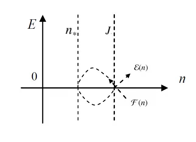
Figure 3. The trajectory of $E$ and $n$.

Thus, we have

(2.3) $$E^{2}=2n-2b\ln n+\frac{2J^{2}}{n}-\frac{bJ^{2}}{n^{2}}+2C_{0}\buildrel\Delta\over{=}g(n),$$

with $g(n_{*})=0$, where $0<n_{*}<n<+\infty$.

Let us use $\mathcal{E}(n)$ to denote the trajectory which is from the supersonic region to the subsonic region, and use $\mathcal{F}(n)$ to stand for the other which has a reverse direction (see Figure 3). In the following, we only consider the $C^{1}$-smooth transonic solution corresponding to $\mathcal{E}(n)$. For this end, we want to investigate the properties of $\mathcal{E}(n)$ to remove the singularity of the targeted equations.

Obviously, from (2.3), we have

(2.4) $$E(n)=\left\{\begin{split}-\sqrt{g(n)},\quad n\leq J,\\ \sqrt{g(n)},\quad n\geq J.\end{split}\right.$$

Here $g(n)$ satisfies $g(J)=0$ and

(2.5) $$\left.\frac{dg}{dn}\right|_{n=J}=\left(2-\frac{2b}{n}-\frac{2J^{2}}{n^{2}}+2\frac{bJ^{2}}{n^{3}}\right)_{n=J}=0,$$

(2.6) $$\left.\frac{d^{2}g}{dn^{2}}\right|_{n=J}=\left(\frac{2b}{n^{2}}+\frac{4J^{2}}{n^{3}}-6\frac{bJ^{2}}{n^{4}}\right)_{n=J}=\frac{4}{J}\left(1-\frac{b}{J}\right)>0,$$

and

(2.7) $$\frac{d^{3}g}{dn^{3}}(n)=-\frac{4}{n^{3}}\left(b+\frac{3J^{2}}{n}-\frac{6bJ^{2}}{n^{2}}\right)\buildrel\Delta\over{=}h(n,b),$$

where we have used the supersonic doping profile condition $b<J$.

Then it follows from the facts $g(n)\in C^{\infty}(n_{*},\infty)$, (2.5)-(2.7) and the Taylor’s formula with the integral remainder, that

$$\begin{split}g(n)=\ &g(J)+(n-J)\left.\frac{dg}{dn}\right|_{n=J}+\frac{(n-J)^{2}}{2}\left.\frac{d^{2}g}{dn^{2}}\right|_{n=J}+\frac{(n-J)^{3}}{2}\int_{0}^{1}(1-t)^{2}\frac{d^{3}g}{dn^{3}}(J+t(n-J))dt\\ =\ &\frac{(n-J)^{2}}{2}\frac{4}{J}\left(1-\frac{b}{J}\right)+\frac{(n-J)^{3}}{2}\int_{0}^{1}(1-t)^{2}\frac{d^{3}g}{dn^{3}}(J+t(n-J))dt\\ =\ &(n-J)^{2}\left(\frac{2}{J}\left(1-\frac{b}{J}\right)+\frac{n-J}{2}\int_{0}^{1}(1-t)^{2}h(J+t(n-J),b)dt\right),\end{split}$$

which implies

(2.8) $$E(n)\buildrel\Delta\over{=}(n-J)W(n,b),$$

where

(2.9) $$W(n,b)=\sqrt{\frac{2}{J}\left(1-\frac{b}{J}\right)+\frac{n-J}{2}\int_{0}^{1}(1-t)^{2}h(J+t(n-J),b)dt}.$$

It is easy to see that $W(n,b)$ has the following properties.

Lemma 2.1.

For $M>n_{*}$ and $0<\varepsilon<J$, there exist positive constants $C_{1}$ and $C_{2}$ depend only on $\varepsilon$ and $M$ such that

(2.10) $$0<C_{1}<W(n,b)<C_{2},\quad for~{}~{}n\in(n_{*},M)~{}~{}and~{}~{}b\in(\varepsilon,J).$$

Moreover, it holds

$$W(n,b)\in C^{\infty}((n_{*},M)\times(\varepsilon,J)),$$

and

$$|\partial_{n}W(n,b)|<C,\quad|\partial_{b}W(n,b)|<C,\quad for~{}~{}n\in(n_{*},M),~{}~{}and~{}~{}b\in(\varepsilon,J).$$

Now, we are going to investigate the structural stability of the $C^{1}$-smooth transonic steady-states.

For $i=1,2$, let $(n_{i},E_{i})$ be the two $C^{1}$-smooth transonic steady-states satisfying

(2.11) $$\left\{\begin{split}&n_{ix}=\frac{n_{i}^{3}}{n_{i}+J}\frac{E_{i}}{n_{i}-J}=\frac{n_{i}^{3}}{n_{i}+J}W(n_{i},b_{i}),\\ &E_{ix}=n_{i}-b_{i},\quad x\in[0,L],\\ &n_{i}(0)=n_{i0},\quad E_{i}(0)=E_{i0},\end{split}\right.$$

where $0<n_{i0}<J,E_{i0}=\mathcal{E}(n_{i0})$.

Lemma 2.2.

There exists a constant $C>0$ such that

(2.12) $$\|n_{1}(\cdot)-n_{2}(\cdot)\|_{C^{1}[0,L]}+\|E_{1}(\cdot)-E_{2}(\cdot)\|_{C^{2}[0,L]}\leq C\delta_{0},$$

where $\delta_{0}$ is the same meaning as that in (1.15).

Proof. By making difference of (2.11) with respect to $n_{1}$ and $n_{2}$, we get

$$\left\{\begin{split}&\left(n_{1}-n_{2}\right)_{x}=\frac{n_{1}^{3}}{n_{1}+J}W(n_{1},b_{1})-\frac{n_{2}^{3}}{n_{2}+J}W(n_{2},b_{2}),\\ &\left(n_{1}-n_{2}\right)(0)=n_{10}-n_{20},\quad x\in[0,L].\end{split}\right.$$

Then, by Lemma 2.1, we have

(2.13) $$\begin{split}\left(n_{1}-n_{2}\right)_{x}=&\left(\frac{n_{1}^{3}}{n_{1}+J}-\frac{n_{2}^{3}}{n_{2}+J}\right)W(n_{1},b_{1})+\frac{n_{2}^{3}}{n_{2}+J}\left(W(n_{1},b_{1})-W(n_{2},b_{2})\right)\\ \leq&C\left|n_{1}-n_{2}\right|+C\left|b_{1}-b_{2}\right|,\end{split}$$

which implies

$$\frac{d\left(n_{1}-n_{2}\right)^{2}}{dx}\leq C\left(\left|n_{1}-n_{2}\right|^{2}+\left|b_{1}-b_{2}\right|^{2}\right),$$

where the Cauchy-Schwarz inequality was used. Following the same way, we find that (2.13) is also true for $n_{2}-n_{1}$. Therefore, it follows that

(2.14) $$\begin{split}\left(n_{1}-n_{2}\right)^{2}\leq C\left(\left|n_{10}-n_{20}\right|^{2}+\left|b_{1}-b_{2}\right|^{2}\right),\quad x\in[0,L],\end{split}$$

namely

(2.15) $$\left|n_{1}-n_{2}\right|\leq C\left(\left|n_{10}-n_{20}\right|+\left|b_{1}-b_{2}\right|\right)\quad x\in[0,L].$$

This together with (2.13) yields

(2.16) $$\left|(n_{1}-n_{2})_{x}\right|\leq C\left(\left|n_{10}-n_{20}\right|+\left|b_{1}-b_{2}\right|\right),\quad x\in[0,L].$$

On the other hand, from the second equation of (2.11), we obtain

(2.17) $$E_{i}(x)=E_{i0}+\int_{0}^{x}\left(n_{i}(y)-b_{i}\right)dy,\quad i=1,2.$$

Then it follows that

(2.18) $$\left|{{E_{1}}(x)-{E_{2}}(x)}\right|\leq \left|{{E_{10}}-{E_{20}}}\right|+\int_{0}^{x}{}\left|{{n_{1}}(y)-{n_{2}}(y)}\right|dy+x\left|{{b_{1}}-{b_{2}}}\right|$$

$$\leq \left|{{E_{10}}-{E_{20}}}\right|+C\mathop{\sup}\limits_{y\in[0,L]}\left|{{n_{1}}(y)-{n_{2}}(y)}\right|+\left|{{b_{1}}-{b_{2}}}\right|$$

$$\leq C\delta_{0},\quad x\in[0,L],$$

(2.19) $$|E_{1x}(x)-E_{2x}(x)|=|n_{1}(x)-n_{2}(x)-(b_{1}-b_{2})|\leq C\delta_{0},,\quad x\in[0,L],$$

and

(2.20) $$|E_{1xx}(x)-E_{2xx}(x)|=|n_{1x}(x)-n_{2x}(x)|\leq C\delta_{0},\quad x\in[0,L].$$

Therefore, by combining (2.15)- (2.16) and (2.18)- (2.20), we obtain

$$\|n_{1}(\cdot)-n_{2}(\cdot)\|_{C^{1}[0,L]}+\|E_{1}(\cdot)-E_{2}(\cdot)\|_{C^{2}[0,L]}\leq C\delta_{0}.$$

The proof of Lemma 2.2 is completed. $\Box$

2.2. Case 2. $\alpha>0$ (i.e., $0<\tau<+\infty$)

In this subsection, we continue to study the following problem with $\alpha>0$

(2.21) $$\begin{cases}\left(n+\displaystyle{\frac{J^{2}}{n}}\right)_{x}=nE-\alpha J,&x\in[0,L],\\ E_{x}=n-b,&x\in[0,L],\\ (n,E)|_{x=0}=(n_{0},E_{0}).\end{cases}$$

Obviously, the first equation of (2.21) can be rewritten as

(2.22) $$\frac{(n-J)(n+J)}{n^{2}}n_{x}=nE-\alpha J\buildrel\Delta\over{=}n\tilde{E},$$

where

$$\tilde{E}=\tilde{E}(n,b):=E-\frac{\alpha J}{n}.$$

In view of (2.22) and

(2.23) $$\tilde{E}_{x}=E_{x}+\frac{\alpha J}{n^{2}}n_{x}=n-b+\frac{\alpha J}{n^{2}}n_{x},$$

it follows that the unknowns $(n,\tilde{E})$ satisfies

(2.24) $$\left\{\begin{split}&n_{x}=\frac{n^{3}}{n+J}\frac{\tilde{E}}{n-J},\\ &\tilde{E}_{x}=n-b+\frac{\alpha J}{n^{2}}n_{x}.\end{split}\right.$$

Then the corresponding trajectory equation to system (2.24) is

(2.25) $$\frac{d\tilde{E}}{dn}=\frac{(n+J)(n-b)(n-J)}{n^{3}\tilde{E}}+\frac{\alpha J}{n^{2}}=\frac{(n+J)(n-b)}{n^{3}}\frac{1}{\frac{\tilde{E}}{n-J}}+\frac{\alpha J}{n^{2}}.$$

It follows from [41] that Euler-Poisson system (2.24) or (2.25) possesses two $C^{\infty}$-smooth transonic solutions. One is denoted by $\tilde{\mathcal{E}}(n)$ which is from supersonic region to subsonic region, and the other is $\tilde{\mathcal{F}}(n)$ which has the inverse direction. In the following, we only consider the $C^{1}$-smooth transonic solution $\tilde{\mathcal{E}}(n)$. Let $\tilde{E}=\tilde{E}(n)=\tilde{E}(n,b)$ be the trajectory corresponding to $\tilde{\mathcal{E}}(n)$. Then from [41], the property of $\tilde{E}(n,b)$ is stated as follows.

Lemma 2.3.

$\tilde{E}(n,b)$ is smooth respect to $n$, and is continuous about $b$. Namely,

$$\tilde{E}(n,b)\in C^{\infty}(n_{*},\infty)\times C^{0}(0,J),$$

where $n_{*}$ satisfies $\tilde{E}(n_{*},b)=0$ and $0<n_{*}<J$.

Set

$$\lim\limits_{n\to J}\frac{d\tilde{E}(n)}{dn}=k.$$

By (2.25) and the Hospital’s rule, we have

$$k=\frac{2(J-b)}{J^{2}}\frac{1}{k}+\frac{\alpha}{J},$$

which implies that

(2.26) $$k=k_{\pm}=\frac{1}{2}\left(\frac{\alpha}{J}\pm\sqrt{\left(\frac{\alpha}{J}\right)^{2}+\frac{8(J-b)}{J^{2}}}\right).$$

Since the targeted trajectory is $\tilde{\mathcal{E}}(n)$ and $b<J$, we get $k=k_{+}>0.$

In order to prove the stability of $C^{1}$-smooth transonic solution, the analysis of properties of $\frac{\tilde{E}}{n-J}$ is crucial due to (2.24). Particularly, we have to investigate the property of $\frac{\tilde{E}}{n-J}$ about the parameter $b$.

In what follows, let us denote

$$\frac{\tilde{E}}{n-J}=\tilde{W}(n,b).$$

Then, in the similar fashion in [41], we have

Lemma 2.4.

For $0<b<J$, $\tilde{W}(n,b)$ is smooth respect to $n$, and is continuous about $b$. Moreover, there exist constants $M=n(L)>n_{*}$ and $C=C(M,b)>0$ such that

$$|\tilde{W}(n,b)|<C,\quad\forall n\in[n_{*},M],$$

and

$$\left|\frac{d\tilde{W}(n,b)}{dn}\right|<C,\quad\forall n\in[n_{*},M],$$

where $n_{*}$ is the same meaning as that in Lemma 2.3.

Remark 2.1.

To prove the property of $\tilde{W}(n,b)$ about the parameter $b$ is key but difficult. In the case of $\alpha=\frac{1}{\tau}=0$, the proof of the property about $W(n,b)$ is easy since it has an explicit formula. However, $\tilde{W}(n,b)$ doesn’t has the explicit representation due to the fact that (2.25) is not separated type.

Next, we begin to establish some necessary estimates and to prove that $\tilde{W}(n,b)$ is Lipschitz continuous with respect to the parameter $b$ as follows,

Lemma 2.5.

For $0<b_{1},b_{2}<J$, there exists constant $C>0$ such that

(2.27) $$\left|\tilde{W}(n,b_{1})-\tilde{W}(n,b_{2})\right|\leq C|b_{1}-b_{2}|,\quad\forall n\in[n_{*},M].$$

Proof. For $h>0$, by choosing $b_{1}=b+h$ and $b_{2}=b$, it follows from (2.25) that

$$\frac{d\tilde{E}(n,b+h)}{dn}=\frac{(n+J)\left(n-(b+h)\right)(n-J)}{n^{3}\tilde{E}(n,b+h)}+\frac{\alpha J}{n^{2}},$$

and

$$\frac{d\tilde{E}(n,b)}{dn}=\frac{(n+J)\left(n-b\right)(n-J)}{n^{3}\tilde{E}(n,b)}+\frac{\alpha J}{n^{2}}.$$

By taking difference of the above two equations, we have

$$\frac{d}{dn}({\tilde{E}}(n,b+h)-{\tilde{E}}(n,b))$$

$$=\left(\frac{(n+J)\left(n-(b+h)\right)(n-J)}{n^{3}\tilde{E}(n,b+h)}-\frac{(n+J)\left(n-b\right)(n-J)}{n^{3}\tilde{E}(n,b+h)}\right)$$

$$\ \ \ +\left(\frac{(n+J)\left(n-b\right)(n-J)}{n^{3}\tilde{E}(n,b+h)}-\frac{(n+J)\left(n-b\right)(n-J)}{n^{3}\tilde{E}(n,b)}\right)$$

$$=\frac{n+J}{n^{3}}\frac{1}{\frac{\tilde{E}(n,b+h)}{n-J}}\left(-h\right)+\frac{(n+J)\left(n-b\right)}{n^{3}}\left(\frac{n-J}{\tilde{E}(n,b+h)}-\frac{n-J}{\tilde{E}(n,b)}\right)$$

$$=\frac{n+J}{n^{3}}\frac{1}{\frac{\tilde{E}(n,b+h)}{n-J}}\left(-h\right)+\frac{(n+J)\left(n-b\right)}{n^{3}}\frac{(n-J)^{2}}{\tilde{E}(n,b+h)\tilde{E}(n,b)}\frac{\tilde{E}(n,b)-\tilde{E}(n,b+h)}{n-J}$$

$$=\frac{n+J}{n^{3}}\frac{1}{\frac{\tilde{E}(n,b+h)}{n-J}}\left(-h\right)+\frac{(n+J)\left(n-b\right)}{n^{3}}\frac{1}{\frac{\tilde{E}(n,b+h)}{n-J}\frac{\tilde{E}(n,b)}{n-J}}\frac{\tilde{E}(n,b)-\tilde{E}(n,b+h)}{n-J}.$$

Dividing (2.2) by $h$, and letting

$$\frac{\tilde{E}(n,b+h)-\tilde{E}(n,b)}{h}\buildrel\Delta\over{=}\Delta_{h}^{b}\tilde{E}(n,b),$$

we obtain

$$\frac{d\left(\Delta_{h}^{b}\tilde{E}(n,b)\right)}{dn}\buildrel\Delta\over{=}f(n,b,h)-g(n,b,h)\frac{\Delta_{h}^{b}\tilde{E}(n,b)}{n-J},$$

where

$$f(n,b,h)=-\frac{n+J}{n^{3}}\frac{1}{\frac{\tilde{E}(n,b+h)}{n-J}},\quad g(n,b,h)=\frac{(n+J)(n-b)}{n^{3}}\frac{1}{\frac{\tilde{E}(n,b)}{n-J}}\frac{1}{\frac{\tilde{E}(n,b+h)}{n-J}}.$$

Set

$$\Delta_{h}^{b}\tilde{E}(n,b)=\mathcal{P}_{h}(n,b)=\mathcal{P},$$

then it follows

(2.29) $$\frac{d\mathcal{P}}{dn}\buildrel\Delta\over{=}f(n,b,h)-g(n,b,h)\frac{\mathcal{P}}{n-J}.$$

We also deduce from $\left.\tilde{E}(n,b)\right|_{n=J}=0$ and $\left.\tilde{E}(n,b+h)\right|_{n=J}=0$ that

(2.30) $$\left.\mathcal{P}\right|_{n=J}=\left.\mathcal{P}_{h}(n,b)\right|_{n=J}=0.$$

Now, we formally suppose that

$$\lim\limits_{n\to J}\frac{d\mathcal{P}}{dn}=l,$$

then by the Hospital’s rule in form, we have

$$l=f(J,b,h)-g(J,b,h)l.$$

It is easy to see that

$$l=\frac{f(J,b,h)}{1+g(J,b,h)}<0,$$

and

$$l\to l_{0}\buildrel\Delta\over{=}\frac{f(J,b)}{1+g(J,b)},\quad{\rm as}\quad h\to 0.$$

On the other hand, by (2.26) we obtain

(2.31) $$\begin{split}&f(n,b,h)\to f(J,b,h)<0,\quad{\rm as}\quad n\to J,\\ &g(n,b,h)\to g(J,b,h),\quad{\rm as}\quad n\to J,\end{split}$$

and

$$\begin{split}&f(n,b,h)\to f(n,b,0)<0,\quad{\rm as}\quad h\to 0,\\ &g(n,b,h)\to g(n,b,0),\quad{\rm as}\quad h\to 0,\\ &g(J,b,h)>C>0,\quad g(n,b,h)>C>0.\end{split}$$

Next we make singularity analysis on problem (2.29)-(2.29) with respect to $n$ in a small neighborhood around the singularity point $n=J$. With the help of the same methods in [41], we want to prove that $\frac{\mathcal{P}}{n-J}$ has not only an upper bound but also a lower bound.

We claim that there exist two positive constants $\varepsilon_{*}$ and $\delta_{*}$ independent of $b$ such that

$$l-\delta_{*}<\frac{\mathcal{P}}{n-J}<l+\delta_{*},\quad\forall n\in[J-\varepsilon_{*},J+\varepsilon_{*}].$$

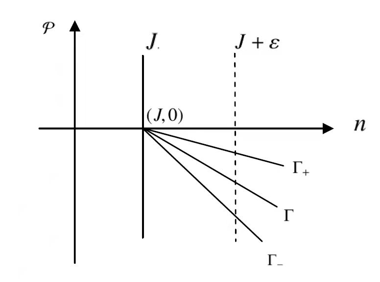
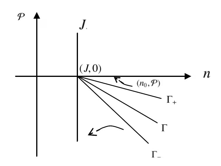
Figure 4. Sketched graph of $\mathcal{P}$ and $n$ near the singular point.

Indeed, we let $\Gamma_{+},\Gamma$ and $\Gamma_{-}$ be three rays which pass through the point $(J,0)$ with the slope values $l+\delta_{*}$, $l$ and $l-\delta_{*}$, respectively. We use $\Sigma_{\varepsilon}$ to stand for the triangle area bounded by rays $\Gamma_{+},\Gamma_{-}$ and the straight line $n=J+\varepsilon$ (see Figure 4). We would like to show that there exists a positive constant $\varepsilon_{+}$ suitable small such that $\mathcal{P}$ must be in $\Sigma_{\varepsilon_{+}}$ as $n\in[J,J+\varepsilon_{+}]$.

We use the method of proof by contradiction. For any $n_{0}\in[J,J+\varepsilon]$, we assume that there always exists one point $(n_{0},\mathcal{P})$ which is lying above the triangle area $\Sigma_{\varepsilon}$.

At $n=n_{0}$, it follows from (2.29) that

$$\frac{d\mathcal{P}}{dn}=f(n,b,h)-g(n,b,h)\frac{\mathcal{P}}{n-J}.$$

This together with $\frac{\mathcal{P}}{n-J}>l+\delta_{*}$ gives

$$\begin{split}\frac{{d\mathcal{P}}}{{dn}}({n_{0}})=&f({n_{0}},b,h)-g({n_{0}},b,h)\frac{\mathcal{P}}{{{n_{0}}-J}}\\ \leq&f({n_{0}},b,h)-g({n_{0}},b,h)(l+\delta_{*})\\ \leq&f(J,b,h)-g(J,b,h)l\\ =&l<l+\delta_{*}.\end{split}$$

This deduces that the trajectory pass through $(n_{0},\mathcal{P}(n_{0}))$ will intersect with the $n-$axis before $n=J$ (see Figure 5). However, this yields a contradiction with $\mathcal{P}(J)=0$. Therefore, we obtain that there must exist constant $\varepsilon_{+}>0$ such that $(n,\mathcal{P})\in\Sigma_{\varepsilon_{+}}$ for any $n\in[J,J+\varepsilon_{+}]$. Furthermore,

$$\frac{\mathcal{P}}{n-J}\in[l-\delta_{*},l+\delta_{*}],\quad\forall n\in[J,J+\varepsilon_{+}].$$

Obviously, the above process holds independent of $b$ and provided that $h>0$ is suitable small. Similarly, we can prove that there must exist constant $\varepsilon_{-}>0$ suitable small such that $(n,\mathcal{P})\in\Sigma_{\varepsilon_{-}}$ for any $n\in[J-\varepsilon_{-},J]$, which implies, $\frac{\mathcal{P}}{n-J}\in[l-\delta_{*},l+\delta_{*}],~{}~{}\forall n\in[J-\varepsilon_{-},J].$

By letting

$$\varepsilon_{*}=\min\{\varepsilon_{+},\varepsilon_{-}\},$$

we obtain

$$l-\delta_{*}\leq\frac{\mathcal{P}}{n-J}\leq l+\delta_{*},\quad\forall n\in[J-\varepsilon_{*},J+\varepsilon_{*}].$$

On the other hand, since (2.29) has no singularity on the domain $[n_{*},J-\varepsilon_{*}]\cup[J+\varepsilon_{*},M]$, it is easy to get

$$\left|\frac{\mathcal{P}}{n-J}\right|<C,\quad\forall n\in[n_{*},J-\varepsilon_{*}]\cup[J+\varepsilon_{*},M].$$

Hence, it follows that

$$\left|\frac{\mathcal{P}}{n-J}\right|<C,\quad\forall n\in[n_{*},M],$$

which implies that

$$\left|\frac{\Delta_{h}^{b}\tilde{E}(n,b)}{n-J}\right|<C,\quad\forall n\in[n_{*},M],$$

namely,

$$\left|\frac{\tilde{E}(n,b+h)-\tilde{E}(n,b)}{n-J}\right|<Ch,\quad\forall n\in[n_{*},M],$$

which gives (2.27). The proof of Lemma 2.5 is completed. $\Box$

Based on the primary works above, we begin to prove the stability of the $C^{1}$-smooth transonic solution as follows.

Lemma 2.6.

There exists a constant $C>0$ such that

(2.32) $$\|n_{1}(\cdot)-n_{2}(\cdot)\|_{C^{1}[0,L]}+\|E_{1}(\cdot)-E_{2}(\cdot)\|_{C^{2}[0,L]}\leq C\delta_{0}.$$

Proof. By plugging $(n,\tilde{E},b)=(n_{1},\tilde{E}(n_{1},b_{1}),b_{1})$ and $(n,\tilde{E},b)=(n_{2},\tilde{E}(n_{2},b_{2}),b_{2})$ into (2.24), respectively. And taking difference of the resulted equations, we have

$$\begin{split}\left(n_{1}-n_{2}\right)_{x}=&\frac{n_{1}^{3}}{n_{1}+J}\frac{\tilde{E}(n_{1},b_{1})}{n_{1}-J}-\frac{n_{2}^{3}}{n_{2}+J}\frac{\tilde{E}(n_{2},b_{2})}{n_{2}-J}\\ =&\frac{n_{1}^{3}}{n_{1}+J}\frac{\tilde{E}(n_{1},b_{1})}{n_{1}-J}-\frac{n_{2}^{3}}{n_{2}+J}\frac{\tilde{E}(n_{1},b_{1})}{n_{1}-J}+\frac{n_{2}^{3}}{n_{2}+J}\frac{\tilde{E}(n_{1},b_{1})}{n_{1}-J}-\frac{n_{2}^{3}}{n_{2}+J}\frac{\tilde{E}(n_{2},b_{2})}{n_{2}-J}\\ =&\frac{\tilde{E}(n_{1},b_{1})}{n_{1}-J}\left(\frac{n_{1}^{3}}{n_{1}+J}-\frac{n_{2}^{3}}{n_{2}+J}\right)+T(n_{1},n_{2},b_{1},b_{2}),\end{split}$$

where

$$\begin{split}T(n_{1},n_{2},b_{1},b_{2})=&\frac{n_{2}^{3}}{n_{2}+J}\left(\frac{\tilde{E}(n_{1},b_{1})}{n_{1}-J}-\frac{\tilde{E}(n_{2},b_{1})}{n_{2}-J}+\frac{\tilde{E}(n_{2},b_{1})}{n_{2}-J}-\frac{\tilde{E}(n_{2},b_{2})}{n_{2}-J}\right).\end{split}$$

By using Lemma 2.4 and the estimate (2.27) in Lemma 2.5, we have

$$\begin{split}T(n_{1},n_{2},b_{1},b_{2})=&\frac{n_{2}^{3}}{n_{2}+J}\left(\frac{d\left(\frac{\tilde{E}(n_{1},b_{1})}{n_{1}-J}\right)}{n}(n=\xi)(n_{1}-n_{2})+\frac{\tilde{E}(n_{2},b_{1})-\tilde{E}(n_{2},b_{2})}{(n_{2}-J)(b_{1}-b_{2})}(b_{1}-b_{2})\right)\\ \leq&C\left|n_{1}-n_{2}\right|+C\left|b_{1}-b_{2}\right|,\end{split}$$

where $\xi$ is a number between $n_{1}$ and $n_{2}$.

Then, by Lemma 2.4 again, we have

$$\begin{split}\left|n_{1}-n_{2}\right|_{x}\leq&\frac{\tilde{E}(n_{1},b_{1})}{n_{1}-J}\left(\frac{n_{1}^{3}}{n_{1}+J}-\frac{n_{2}^{3}}{n_{2}+J}\right)+C\left|n_{1}-n_{2}\right|+C\left|b_{1}-b_{2}\right|\\ \leq&C\left|n_{1}-n_{2}\right|+C\left|b_{1}-b_{2}\right|,\end{split}$$

which implies

$$\frac{d\left(n_{1}-n_{2}\right)^{2}}{dx}\leq C\left(\left|n_{1}-n_{2}\right|^{2}+\left|b_{1}-b_{2}\right|^{2}\right),$$

where the Cauchy-Schwarz inequality was used. Therefore, it follows that

$$\begin{split}\left(n_{1}-n_{2}\right)^{2}\leq C\left(\left|n_{10}-n_{20}\right|^{2}+\left|b_{1}-b_{2}\right|^{2}\right),\quad x\in[0,L],\end{split}$$

i.e.

$$\begin{split}\left|n_{1}-n_{2}\right|\leq C\left(\left|n_{10}-n_{20}\right|+\left|b_{1}-b_{2}\right|\right)\quad x\in[0,L].\end{split}$$

On the other hand, from the second equation of (2.21), we obtain

$$\begin{split}E_{i}(x)=E(n_{i},b_{i})=E_{i0}+\int_{0}^{x}\left(n_{i}(y)-b_{i}\right)dy,\quad i=1,2.\end{split}$$

Then it follows that (2.18)- (2.20) are also true for $\alpha>0$. Namely, we prove

$$\|n_{1}(\cdot)-n_{2}(\cdot)\|_{C^{1}[0,L]}+\|E_{1}(\cdot)-E_{2}(\cdot)\|_{C^{2}[0,L]}\leq C\delta_{0}.$$

The proof of Lemma 2.6 is completed. $\Box$

Finally, by combining Lemma 2.2 and Lemma 2.6, we immediately prove the structural stability of $C^{1}$-smooth transonic steady-states of (1.8) on $[0,L]$ in Theorem 1.2.

3. Structural stability for steady transonic shock solutions

In this section, we mainly prove Theorem 1.4 and establish the structural stability for steady transonic shock solutions. Since Theorem 1.5 can be similarly obtained, we omit its proof.

3.1. Preliminaries

First, we prove the monotonic relation between the shock position and the downstream density and a priori estimates for the steady flows, which play a crucial role for the proof of Theorem 1.4. For any supersonic state $(n,E)$ satisfying $n<J$ , we can connect it to a unique subsonic state $(\mathscr{S}(n),E)$ via a transonic shock. Here $\mathscr{S}(n)$ is determined by the entropy condition and the Rankine-Hugoniot condition

(3.1) $$\mathscr{S}(n)+\frac{{{J^{2}}}}{{\mathscr{S}(n)}}=n+\frac{{{J^{2}}}}{n},\quad{\rm and}\quad\mathscr{S}(n)>J.$$

By differentiating (3.1) with respect to $n$, we have

(3.2) $$\frac{{d\mathscr{S}(n)}}{{dn}}=\displaystyle\frac{{1-\displaystyle\frac{{{J^{2}}}}{{{n^{2}}}}}}{{1-\displaystyle\frac{{{J^{2}}}}{{{\mathscr{S}^{2}}(n)}}}}.$$

This together with (1.6) give

(3.3) $$\frac{{d\mathscr{S}(n(x))}}{{dx}}=\frac{{nE-\alpha J}}{{1-\displaystyle\frac{{{J^{2}}}}{{{\mathscr{S}^{2}}(n)}}}}.$$

Lemma 3.1 (Monotonic relation for the transonic shock solutions).

Let $(n^{(1)},E^{(1)})$ and $(n^{(2)},E^{(2)})$ be two transonic shock solutions of (1.6), and $(n^{(i)},E^{(i)})$ $(i=1,2)$ are defined by

$$({{n^{(i)}},{E^{(i)}}})=\left\{{\begin{array}[]{*{20}{c}}\vspace{3mm}{({n_{\rm sup}^{(i)},E_{\rm sup}^{(i)}})(x),\hfill}&{{as}\quad x\in(0,x_{i}),\hfill}\\ {({n_{\rm sub}^{(i)},E_{\rm sub}^{(i)}})(x),\hfill}&{{as}\quad x\in(x_{i},L),\hfill}\\ \end{array}}\right.$$

where

$$n_{\rm sup}^{(i)}<J<n_{\rm sub}^{(i)},\quad{for}\quad i=1,2.$$

They satisfy the same upstream boundary conditions

$${n^{(1)}}(0)={n^{(2)}}(0)={n_{l}},\quad{E^{(1)}}(0)={E^{(2)}}(0)={E_{l}}.$$

Then, if $b<J,{x_{1}}<{x_{2}}$ and $E_{\rm sup}^{(2)}({x_{1}})>0$, we have

$${n^{(1)}}(L)>{n^{(2)}}(L).$$

Proof. For $x\in[0,{x_{1}})$, due to the fact that both $({n_{\sup}^{(1)},E_{\sup}^{(1)}})$ and $({n_{\sup}^{(2)},E_{\sup}^{(2)}})$ satisfy ordinary differential equations (1.6) and the same initial data, we obtain

$$({n_{\sup}^{(1)},E_{\sup}^{(1)}})=({n_{\sup}^{(2)},E_{\sup}^{(2)}}),\quad{\rm as}\quad x\in[0,{x_{1}}).$$

For $x\in[{x_{1}},{x_{2}}]$, we define a function $\mathscr{E}$ as follows

$$\left\{{\begin{array}[]{*{20}{c}}\vspace{3mm}{\displaystyle\frac{{d\mathscr{E}}}{{dx}}=\mathscr{S}({n_{\sup}^{(2)}})-b,\quad{\rm as}\quad x\in[x_{1},x_{2}],\hfill}&\hfill{}\hfil\\ {\mathscr{E}({x_{1}})=E_{\rm sub}^{(1)}({x_{1}})=E_{\sup}^{(1)}({x_{1}})=E_{\sup}^{(2)}({x_{1}}).\hfill}&\hfill{}\hfil\\ \end{array}}\right.$$

In view of $n_{\rm sup}^{(2)}<J<\mathscr{S}({n_{\rm sup}^{(2)}})$, by using the comparison principles for ordinary differential equations [37], we get $E_{\sup}^{(2)}(x)<\mathscr{E}(x)$ as $x\in({x_{1}},{x_{2}}].$ This, together with (3.3), gives

$$\frac{{d\mathscr{S}({n_{\sup}^{(2)}})}}{{dx}}=\frac{{n_{\sup}^{(2)}E_{\sup}^{(2)}-\alpha J}}{{1-\displaystyle\frac{{{J^{2}}}}{{{\mathscr{S}^{2}}(n_{\sup}^{(2)})}}}}<\frac{{n_{\sup}^{(2)}\mathscr{E}(x)-\alpha J}}{{1-\displaystyle\frac{{{J^{2}}}}{{{\mathscr{S}^{2}}(n_{\sup}^{(2)})}}}}.$$

On the other hand, it follows from $\mathscr{E}({x_{1}})=E_{\sup}^{(2)}({x_{1}})>0$ and $b<J<\mathscr{S}({n_{\rm sup}^{(2)}})$ that $\mathscr{E}(x)>0$ as $x\in({x_{1}},{x_{2}}]$, which furthermore gives

$$\left\{{\begin{array}[]{*{20}{c}}\vspace{3mm}{\displaystyle\frac{{d\mathscr{S}({n_{\rm sup}^{(2)}})}}{{dx}}<\displaystyle\frac{{\mathscr{S}({n_{\rm sup}^{(2)}})\mathscr{E}(x)-\alpha J}}{{1-\displaystyle\frac{{{J^{2}}}}{{{\mathscr{S}^{2}}(n_{\rm sup}^{(2)})}}}},\hfill}\\ \vspace{3mm}{\displaystyle\frac{{d\mathscr{E}}}{{dx}}=\mathscr{S}({n_{\rm sup}^{(2)}})-b,\hfill}\\ {\mathscr{S}({n_{\rm sup}^{(2)}})({x_{1}})=n_{\rm sub}^{(1)}({x_{1}}),\mathscr{E}({x_{1}})=E_{\rm sub}^{(1)}({x_{1}}).\hfill}\\ \end{array}}\right.$$

Then, by using the comparison principles for ordinary differential equations again, we have

$$\mathscr{S}\left({n_{\rm sup}^{(2)}}\right)({x_{2}})<n_{\rm sub}^{(1)}({x_{2}}),\quad\mathscr{E}({x_{2}})<E_{\rm sub}^{(1)}({x_{2}}).$$

In view of $E_{\sup}^{(2)}({x_{2}})<\mathscr{E}({x_{2}}),$ we obtain

$$E_{\rm sub}^{(2)}({x_{2}})=E_{\sup}^{(2)}({x_{2}})<\mathscr{E}({x_{2}})<E_{\rm sub}^{(1)}({x_{2}}).$$

Recall that $({n_{\rm sub}^{(1)},E_{\rm sub}^{(1)}})$ and $({n_{\rm sub}^{(2)},E_{\rm sub}^{(2)}})$ solve the same ordinary differential equations on $[x_{2},L]$, by the comparison principle for ordinary differential equations once more, we get

$$n_{\rm sub}^{(1)}(L)>n_{\rm sub}^{(2)}(L),\quad{\rm and}\quad E_{\rm sub}^{(1)}(L)>E_{\rm sub}^{(2)}(L).$$

The proof of Lemma 3.1 is completed. $\Box$

Next, by using the multiplier method, we establish the a priori estimates for supersonic and subsonic flows, which yield the existence of supersonic, subsonic, and transonic shock solutions.

It follows from (1.6) that $n$ satisfies

(3.4) $$\frac{d}{dx}\left({\mathfrak{f}(n)n_{x}+\alpha\displaystyle\frac{J}{{n}}}\right)=n-b,$$

in which $\mathfrak{f}(n)=\displaystyle\frac{n^{2}-J^{2}}{n^{3}}$.

Let $(n_{0},E_{0})$ be a supersonic or subsonic solution of (1.6) with the doping profile $b_{0}$ and with initial data $(n_{I},E_{I})$, i.e.,

(3.5) $$\left\{{\begin{array}[]{*{20}{c}}\vspace{3mm}\displaystyle\frac{d}{dx}\left({\mathfrak{f}(n)n_{x}+\alpha\displaystyle\frac{J}{{n}}}\right)=n-{b_{0}},\hfill\\ {n(a)={n_{I}},\quad n_{x}(a)=\displaystyle\frac{{{E_{I}}-\alpha\displaystyle\frac{J}{{{n_{I}}}}}}{{\mathfrak{f}({n_{I}})}}.\hfill}\\ \end{array}}\right.$$

In the following lemma, we give the stability estimates for both the supersonic and the subsonic solutions of (1.6), which are small perturbations of the solutions to the problem (3.5).

Lemma 3.2.

For any interval $[a,l]\subseteq[0,x_{0})\cup(x_{0},L]$, suppose $(n_{0},E_{0})$ to be a supersonic or subsonic solution to the problem (3.5). Then there is $\epsilon>0$ such that if

(3.6) $${\left\|{b(x)-{b_{0}}}\right\|_{{C^{0}}[a,l]}}+\left|{{{\tilde{n}}_{I}}}\right|+\left|{{{\tilde{E}}_{I}}}\right|<\epsilon,$$

then, for $x\in[a,l]$, there exists a unique supersonic or subsonic solution $(n,E)(x)$ to the problem (1.6) with initial conditions

(3.7) $$n(a)={n_{I}}+{\tilde{n}_{I}},\quad E(a)={E_{I}}+{\tilde{E}_{I}}.$$

Furthermore, $(n,E)$ satisfies

(3.8) $${\left\|{n-{n_{0}}}\right\|_{{C^{1}}[a,l]}}<C{e^{\gamma L}}\epsilon,$$

where constants $C>0$ and $\gamma>0$.

Proof. The proof is given only for the case when $n_{0}$ is supersonic on $[a,l]$ (the case when $n_{0}$ is subsonic is quite similar). When $n_{0}$ is supersonic on $[a,l]$, there exist constants $c_{0}>0$, $c_{1}>0$ and $c_{2}>0$ such that

(3.9) $$\mathfrak{f}\left({{n_{0}}}\right)(x)>{c_{0}},\quad{c_{1}}<{n_{0}}(x)<J,\quad{\rm and}\quad\left|{\frac{d}{dx}n_{0}(x)}\right|\leq{c_{2}},\quad{\rm as}\quad x\in[a,l].$$

First, we prove the results by assuming that

(3.10) $$\mathfrak{f}\left(n\right)(x)>\frac{{{c_{0}}}}{2},\quad\frac{1}{2}{c_{1}}<n(x)<J,\quad{\rm and}\quad\left|\frac{d}{dx}n(x)\right|\leq 2{c_{2}},\quad{\rm as}\quad x\in[a,l].$$

If we get the estimate (3.8), then the lemma can be proved by using the local existence theory of ordinary differential equations and the standard continuation argument.

Set $\tilde{n}=n-{n_{0}}$ and $\tilde{b}=b-{b_{0}}$. Then from (3.4)-(3.5), we obtain

(3.11) $$\frac{d}{dx}\left({\mathfrak{f}(n)\tilde{n}_{x}+{\mathfrak{F}_{1}}({n_{0}},\tilde{n})\tilde{n}\frac{dn_{0}}{dx}+{\mathfrak{F}_{2}}({n_{0}},\tilde{n})\tilde{n}}\right)-\tilde{n}=-\tilde{b},$$

where

$${\mathfrak{F}_{1}}({n_{0}},\tilde{n})=\int_{0}^{L}\frac{d}{dn}\mathfrak{f}({n_{0}}+\theta\tilde{n})d\theta\quad{\rm and}\quad{\mathfrak{F}_{2}}({n_{0}},\tilde{n})=\alpha J\int_{0}^{L}\displaystyle\frac{{-1}}{{{{\left({{n_{0}}+\theta\tilde{n}}\right)}^{2}}}}d\theta.$$

For constant $\mu>0$, we define a multiplier $\mathfrak{K}(x):=e^{-\mu(x-a)}$, and then multiply both sides of (3.11) by $\mathfrak{K}(x)(\tilde{n}_{x}+\tilde{n})$. By an integration by parts, we have

$$\begin{split}&-\int_{a}^{l}\tilde{b}\mathfrak{K}(x)(\tilde{n}_{x}+\tilde{n})dx\\ =&\int_{a}^{l}\mathfrak{K}(x)\left(\left({\frac{\mu}{2}-1}\right)\mathfrak{f}(n)+\frac{1}{2}\frac{d}{dx}\mathfrak{f}(n)+{\mathfrak{F}_{1}}({n_{0}},\tilde{n})\frac{dn_{0}}{dx}+{\mathfrak{F}_{2}}({n_{0}},\tilde{n})\right){(\tilde{n}_{x})^{2}}dx\\ &+\int_{a}^{l}\mathfrak{K}(x)\left({\frac{{{\mu^{2}}}}{2}\mathfrak{f}(n)-\frac{\mu}{2}\frac{d}{dx}\mathfrak{f}(n)+\frac{d}{dx}\left(\mathfrak{F}_{1}({n_{0}},\tilde{n})\frac{dn_{0}}{dx}\right)-1+\frac{d}{dx}\mathfrak{F}_{2}}({n_{0}},\tilde{n})\right){(\tilde{n})^{2}}dx\\ &+\int_{a}^{l}\mathfrak{K}(x)\left({\frac{d}{dx}\left(\mathfrak{F}_{1}({n_{0}},\tilde{n})\frac{dn_{0}}{dx}\right)+\mathfrak{F}_{1}({n_{0}},\tilde{n})\frac{dn_{0}}{dx}-1+\mathfrak{F}_{2}({n_{0}},\tilde{n})+\frac{d}{dx}\mathfrak{F}_{2}({n_{0}},\tilde{n})}\right)\tilde{n}\tilde{n}_{x}dx\\ &+\mathfrak{K}(l){\left[{\mathfrak{f}(n)\frac{{{{(\tilde{n}_{x})}^{2}}}}{2}+\mathfrak{f}(n)\tilde{n}\tilde{n}_{x}+\mu\mathfrak{f}(n)\frac{{{{(\tilde{n})}^{2}}}}{2}}\right]_{x=l}}-{\left[{\mathfrak{f}(n)\frac{{{{(\tilde{n}_{x})}^{2}}}}{2}+\mathfrak{f}(n)\tilde{n}\tilde{n}_{x}+\mu\mathfrak{f}(n)\frac{{{{(\tilde{n})}^{2}}}}{2}}\right]_{x=a}}.\end{split}$$

It follows from (3.10) that we can choose $\mu$ large enough such that

(3.12) $$\int_{a}^{l}\mu{e^{-\mu(x-a)}}\left({\mu{{\tilde{n}}^{2}}+{{\left({\tilde{n}_{x}}\right)}^{2}}}\right)dx+{e^{-\mu(l-a)}}\left({\mu{{\tilde{n}}^{2}}+{{\left({\tilde{n}_{x}}\right)}^{2}}}\right)(l)$$

$$\leq C\int_{a}^{l}{e^{-\mu(x-a)}}{{\tilde{b}}^{2}}dx+C\left({\mu\tilde{n}_{I}^{2}+\tilde{E}_{I}^{2}}\right).$$

On the other hand, from (3.6), we get

$$\int_{a}^{l}{}{e^{-\mu(x-a)}}{\tilde{b}^{2}}dx+C\left({\mu\tilde{n}_{I}^{2}+\tilde{E}_{I}^{2}}\right)\leq C{\epsilon^{2}}.$$

This, together with (3.12), yields

$$\int_{a}^{l}\left({{{\tilde{n}}^{2}}+{{\left({\tilde{n}_{x}}\right)}^{2}}}\right)dx\leq C{e^{\mu(l-a)}}{\epsilon^{2}}\leq C{e^{\mu}}{\epsilon^{2}}.$$

By Sobolev embedding Theorem, it further gives

$$\left\|\tilde{n}\right\|_{C^{0}[a,l]}\leq\left\|\tilde{n}\right\|_{H^{1}[a,l]}\leq C{e^{\gamma L}}\epsilon,$$

where $\gamma=\displaystyle\frac{\mu}{2}.$ Then it follows from (3.11) that

$${\left\|{\tilde{n}_{x}}\right\|_{{C^{0}}[a,l]}}\leq C{e^{\gamma L}}\epsilon.$$

Hence, (3.8) follows by combining the above two inequalities. The proof of the lemma 3.2 is completed. $\Box$

3.2. Structural stability for transonic shock solutions

In this subsection, we begin to prove Theorem 1.4 and establish the structural stability for transonic shock solutions to the boundary value problem (1.6) and (1.9).

Proof of Theorem 1.4. The proof is divided into three stepsn.

Step 1. For $b(x)=b_{0}(x)$ and $i=1,2$, we prove that there exist transonic shock solutions $(n_{i},E_{i})(x)$ with the shock location at $x_{i}$ such that $x_{2}>x_{1}$, and $n_{2}^{r}(L)<{n_{r}}<n_{1}^{r}(L)$.

By the conditions stated in Theorem 1.4 on the unperturbed transonic shock solution $(n^{(0)},E^{(0)})$ for the case when $b(x)=b_{0}(x)(x\in[0,L])$, there is a constant $\delta>0$ which satisfies $[x_{0}-\delta,x_{0}+\delta]\subset(0,L)$, such that the ordinary differential equations

(3.13) $$\begin{split}\frac{d}{dx}{\left({n+\frac{{{J^{2}}}}{n}}\right)}=nE-\alpha J,\quad{E_{x}}=n-{b_{0}},\end{split}$$

with the initial condition

(3.14) $$\begin{split}(n,E)\left|\right._{x=0}=(n_{l},E_{l}),\end{split}$$

have a unique smooth solution $(n^{l},E^{l})(x)$ on the interval $x\in[0,x_{0}+\delta]$ which satisfies $0<n^{l}(x)<J$ for $x\in[0,x_{0}+\delta]$ and

(3.15) $$\begin{split}{E^{l}}(x)>0,\quad{\rm for}\quad x\in[x_{0}-\delta,x_{0}+\delta],\end{split}$$

where $x_{0}$ is the shock location for $(n^{(0)},E^{(0)})$ for the case when $b(x)=b_{0}(x\in[0,L])$. Furthermore, it follows from the uniqueness for the initial value problems of ordinary differential equations that

$$(n^{l},E^{l})(x)=(n^{(0)},E^{(0)})(x),\quad{\rm as}\quad x\in[0,{x_{0}}).$$

Set ${x_{1}}={x_{0}}-\delta$ and ${x_{2}}={x_{0}}+\delta.$ Then for $x\in[{x_{i}},L]$, let $\left({n_{i}^{r},E_{i}^{r}}\right)(x)(i=1,2)$ be the solution of the ordinary differential equations (3.13) with the initial conditions

$$\ (n_{i}^{r},E_{i}^{r})|_{x=x_{i}}=(\mathscr{S}(n^{l}(x_{i})),E^{l}(x_{i})),\quad{\rm for}\quad i=1,2.$$

We obtain from Lemma 3.2 that there is a unique smooth subsonic solution $(n^{r}_{i},E^{r}_{i})(x)$ on the interval $x\in[x_{i},L]$ satisfying $n^{r}_{i}(x)>n_{s}$ and $E^{r}_{i}(x)>E^{l}(x_{i})>0$ as $x\in(x_{i},L](i=1,2)$. Furthermore, Lemma 3.1 together with $x_{2}>x_{1}$ yield

(3.16) $$\begin{split}n_{2}^{r}(L)<{n_{r}}<n_{1}^{r}(L).\end{split}$$

Step 2. When $b$ is a small perturbation of $b_{0}$, we prove that there exist two transonic shock solutions $(\hat{n}^{(1)},\hat{E}^{(1)})(x)$ and $(\hat{n}^{(2)},\hat{E}^{(2)})(x)$ with the shock location at $x_{1}$ and $x_{2}$, respectively, such that $\hat{n}_{2}^{r}(L)<{n_{r}}<\hat{n}_{1}^{r}(L)$.

For the case that $b$ is a small perturbation of $b_{0}$, we define two transonic solutions based on $\left({n_{1}^{r},E_{1}^{r}}\right)$ and $\left({n_{2}^{r},E_{2}^{r}}\right)$. Let

$$({{{\hat{n}}^{(i)}},{{\hat{E}}^{(i)}}})(x)=\left\{{\begin{array}[]{*{20}{c}}\vspace{3mm}{({\hat{n}_{i}^{l},\hat{E}_{i}^{l}})(x),\hfill}&{{\rm as}\quad x\in[0,x_{i}),\hfill}\\ {({\hat{n}_{i}^{r},\hat{E}_{i}^{r}})(x),\hfill}&{{\rm as}\quad x\in(x_{i},L],\hfill}\\ \end{array}}\right.$$

for $i=1,2,$ where $({\hat{n}_{i}^{l},\hat{E}_{i}^{l}})(x)$ is the solution of the ordinary differential equations

(3.17) $$\begin{split}\frac{d}{dx}{\left({n+\frac{{{J^{2}}}}{n}}\right)}=nE-\alpha J,\quad{E_{x}}=n-b(x),\end{split}$$

on the region $[0,x_{i}]$ with the initial data (3.14) and $(\hat{n}^{r}_{i},\hat{E}^{r}_{i})$ is the solution of the ordinary differential equations (3.17) on $[x_{i},L]$ with the initial data

$$(\hat{n}^{r}_{i},\hat{E}^{r}_{i})|_{x=x_{i}}=({\mathscr{S}({\hat{n}_{i}^{l}({x_{i}}-)}),\hat{E}_{i}^{l}({x_{i}})}).$$

By Lemma 3.2 and (1.19), we obtain that $(\hat{n}_{i}^{l},\hat{E}_{i}^{l})$ and $(\hat{n}_{i}^{r},\hat{E}_{i}^{r})$ are well-defined and satisfy

$$\mathop{\sup}\limits_{x\in[0,{x_{i}})}\left|{({\hat{n}_{i}^{l},\hat{E}_{i}^{l}})-({n_{i}^{l},{E^{l}}})}\right|\leq C\varepsilon,\quad\mathop{\sup}\limits_{x\in({x_{i}},L]}\left|{({\hat{n}_{i}^{r},\hat{E}_{i}^{r}})-({n_{i}^{r},E_{i}^{r}})}\right|\leq C\varepsilon,\quad{\rm for}\quad i=1,2.$$

Furthermore, we have

$$\left|{\hat{n}_{i}^{r}(L)-n_{i}^{r}(L)}\right|\leq C\varepsilon,\quad{\rm for}\quad i=1,2.$$

This, together with (3.16), yields that

$$\hat{n}_{2}^{r}(L)<{n_{r}}<\hat{n}_{1}^{r}(L),$$

provided that $\epsilon>0$ is small enough.

Step 3. We prove that there exists a unique transonic shock solution $(\tilde{n},\tilde{E})$ with a single transonic shock located at a point $\tilde{x}_{0}\in(x_{1},x_{2})$.

The results established in steps 1-2 show that the boundary problem (1.6) and (1.9) admits a unique transonic shock solution $(\tilde{n},\tilde{E})$ with a single transonic shock located at some point $\tilde{x}_{0}\in(x_{1},x_{2})$ by a monotonicity argument as follows: for $x\in[x_{1},x_{2}]$, we define a function $\mathfrak{M}(x)=n(L)$ where $n$ is a transonic shock solution of the system (1.6) satisfying (3.14) with shock located at $x$. By Lemmas 3.1-3.2, we obtain that $\mathfrak{M}(x)$ is continuous strictly decreasing on $[x_{1},x_{2}]$. Furthermore, it follows from the stability estimate (3.8) in Lemma 3.2 that $\tilde{x}_{0}\in[x_{0}-C\epsilon,x_{0}+C\epsilon]$. We have completed the proof of Theorem 1.4. $\Box$

4. Linear dynamic instability of transonic shock solutions

In this section, we study the linear dynamic instability of transonic shock solutions for the Euler-Poisson equations with relaxation effect (1.1).

4.1. Formulation of the linearized problem

Let $(\bar{n},\bar{u},\bar{E})$ be a steady transonic shock solution of the form (1.20) which satisfies (1.33). Assume that the initial values $(n_{0},u_{0},E_{0})$ satisfy (1.29) and the compatibility conditions. From [30], we obtain that there is a piecewise smooth solution containing a single shock $x=s(t)$ (with $s(0)=\tilde{x}_{0})$ which satisfies the Rankine-Hugoniot conditions (1.32) and the Lax geometric shock condition, of the Euler-Poisson equations with relaxation effect on $[0,\bar{T}]$ for some $\bar{T}>0$, which can be written in the following form

(4.1) $$\begin{split}(n,u,E)(t,x)=\left\{{\begin{array}[]{*{20}{c}}\vspace{3mm}{({n_{-}},{u_{-}},{E_{-}}),\hfill}&{{\rm as}\quad x\in(0,s(t)),\hfill}\\ {({n_{+}},{u_{+}},{E_{+}}),\hfill}&{{\rm as}\quad x\in(s(t),L).\hfill}\\ \end{array}}\right.\end{split}$$

By noting that, when $t>T_{0}$ for some $T_{0}>0$, $(n_{-},u_{-},E_{-})$ will depend only on the boundary values at $x=0$. Furthermore, when $\varepsilon$ is small, by the standard lifespan argument in [30], we get $T_{0}<\bar{T}$. Hence,

(4.2) $$\begin{split}({n_{-}},{u_{-}},{E_{-}})=({\bar{n}_{-}},{\bar{u}_{-}},{\bar{E}_{-}})\quad{\rm as}\quad t>{T_{0}}.\end{split}$$

In what follows, we set $T_{0}=0$ for convenience. We would like to extend the local-in-time solution to all $t>0$. Note (4.2), we need only to establish uniform estimates in the region $\{(t,x)|t>0,x>s(t)\}$. To this end, let us formulate an initial boundary value problem in this region. Obviously, the Rankine-Hugoniot conditions for (4.1) are

(4.3) $$\begin{split}[nu]=[n]s^{\prime}(t),\quad\left[n+{n{u^{2}}}\right]=[nu]s^{\prime}(t),\end{split}$$

where $[g]=g\left({t,s(t)^{+}}\right)-g\left({t,s(t)^{-}}\right)$ is the jump of $g(t,x)$ at $x=s(t)$.

From (4.3), we have $\left[{n+n{u^{2}}}\right]\times[n]={\left[{nu}\right]^{2}}.$ That is

$$\left({n_{+}+\frac{{J_{+}^{2}}}{{{n_{+}}}}-n_{-}-\frac{{J_{-}^{2}}}{{{n_{-}}}}}\right)\left({{n_{+}}-{n_{-}}}\right)\left({t,s(t)}\right)={\left({{J_{+}}-{J_{-}}}\right)^{2}}\left(t,s(t)\right),$$

where $J=nu$, $J_{+}=n_{+}u_{+}$ and $J_{-}=n_{-}u_{-}$. By noting (4.2), we get

(4.4) $$\begin{split}J\left({t,s(t)^{-}}\right)=\bar{J}.\end{split}$$

Therefore, we obtain

$$\begin{split}&\left({{n_{+}}\left({t,s(t)}\right)-{n_{-}}\left({s(t)}\right)}\right)\times\\ &\left({n_{+}\left({t,s(t)}\right)\!+\!\frac{{J_{+}^{2}\left({t,s(t)}\right)}}{{{n_{+}}\left({t,s(t)}\right)}}\!-\!{\bar{n}}_{+}\left({s(t)}\right)\!-\!\frac{{{{\bar{J}}^{2}}}}{{{{\bar{n}}_{+}}}}\left({s(t)}\right)}\!+\!{\bar{n}}_{+}\left({s(t)}\right)\!+\!\frac{{{{\bar{J}}^{2}}}}{{{{\bar{n}}_{+}}}}\left({s(t)}\right)\!-\!{\bar{n}}_{-}\left({s(t)}\right)\!-\!\frac{\bar{J}^{2}}{{\bar{n}}_{-}}\left(s(t)\right)\right)\\ &={\left({{J_{+}}\left({t,s(t)}\right)-\bar{J}}\right)^{2}}.\end{split}$$

By the Rankine-Hugoniot conditions (1.23) and Taylor expansions, we have

$$\begin{split}&\left({{{n_{+}}\left({t,s(t)}\right)-{{\bar{n}}_{+}}\left({s(t)}\right)}-\bar{u}^{2}_{+}\left({s(t)}\right)\left({{n_{+}}\left({t,s(t)}\right)-{{\bar{n}}_{+}}\left({s(t)}\right)}\right)}\right.\\ &\hskip 14.22636pt+2\bar{u}_{+}\left({s(t)}\right)\left({{J_{+}}\left({t,s(t)}\right)-\bar{J}}\right)+{\partial_{x}}\left({{\bar{n}}_{+}+\frac{{{{\bar{J}}^{2}}}}{{{{\bar{n}}_{+}}}}}\right)\left({{x_{0}}}\right)\left({s(t)-{x_{0}}}\right)\\ &\hskip 14.22636pt\left.{-{\partial_{x}}\left({{\bar{n}}_{-}+\frac{{{{\bar{J}}^{2}}}}{{{{\bar{n}}_{-}}}}}\right)\left({{x_{0}}}\right)\left({s(t)-{x_{0}}}\right)+{\mathcal{R}}}\right)\times\left({{{\bar{n}}_{+}}\left({{x_{0}}}\right)-{{\bar{n}}_{-}}\left({{x_{0}}}\right)+{\mathcal{R}}}\right)\\ &={\left({{J_{+}}\left({t,s(t)}\right)-\bar{J}}\right)^{2}},\end{split}$$

where

$${\mathcal{R}}=\mathcal{O}(1)\left({{{\left({{n_{+}}\left(t,s(t)\right)-{{\bar{n}}_{+}}\left({s(t)}\right)}\right)}^{2}}+{{\left({{J_{+}}\left({t,s(t)}\right)-\bar{J}}\right)}^{2}}+{{\left({s(t)-{x_{0}}}\right)}^{2}}}\right).$$

From now on, we usually use $\mathcal{R}$ to stand for those quadratic terms with different $\mathcal{O}(1)$ coefficients. Then it follows from the implicit function Theorem that

(4.5) $$\begin{split}\left({{J_{+}}-\bar{J}}\right)\left({t,s(t)}\right)={\mathcal{M}_{1}}\left({\left({{n_{+}}-{{\bar{n}}_{+}}}\right)\left(t,s(t)\right),s(t)-{x_{0}}}\right),\end{split}$$

where $\mathcal{M}_{1}$ satisfies

$${\mathcal{M}_{1}}\left({0,0}\right)=0,\quad\displaystyle\frac{{\partial{\mathcal{M}_{1}}}}{{\partial\left({{n_{+}}-{{\bar{n}}_{+}}}\right)}}=-\displaystyle\frac{{1-\bar{u}^{2}_{+}}}{{2\bar{u}_{+}}}({x_{0}}),\quad\displaystyle\frac{{\partial{\mathcal{M}_{1}}}}{{\partial\left({s(t)-{x_{0}}}\right)}}=-\displaystyle\frac{{\left({{{\bar{n}}_{+}}-{{\bar{n}}_{-}}}\right){{\bar{E}}_{+}}}}{{2\bar{u}_{+}}}({x_{0}}).$$

By plugging (4.5) into (4.3)₁, we get

(4.6) $$\begin{split}s^{\prime}(t)={\mathcal{M}_{2}}\left({\left({{n_{+}}-{{\bar{n}}_{+}}}\right)\left(t,s(t)\right),s(t)-{x_{0}}}\right),\end{split}$$

where $\mathcal{M}_{2}$ satisfies

$${\mathcal{M}_{2}}\left({0,0}\right)=0,\quad\displaystyle\frac{{\partial{\mathcal{M}_{2}}}}{{\partial\left({{n_{+}}-{{\bar{n}}_{+}}}\right)}}=\frac{\bar{u}^{2}_{+}-1}{{2{{\bar{u}}_{+}}\left({{{\bar{n}}_{+}}-{{\bar{n}}_{-}}}\right)}}({x_{0}}),\quad\displaystyle\frac{{\partial{\mathcal{M}_{2}}}}{{\partial\left({s(t)-{x_{0}}}\right)}}=-\displaystyle\frac{{{{\bar{E}}_{+}}}}{{2{{\bar{u}}_{+}}}}({x_{0}}).$$

From (1.1)₃, we obtain

$${E_{+}}(t,x)={E_{l}}+\int_{0}^{s(t)}{}\left({{n_{-}}-b}\right)(z)dz+\int_{s(t)}^{x}\left({{n_{+}}-b}\right)(z)dz,\quad{\rm as}\quad x\in(s(t),L].$$

It follows from (1.1)₁ and the Rankine-Hugoniot conditions (4.3) that

$${\partial_{t}}{E_{+}}={n_{l}}{u_{l}}-{n_{+}}{u_{+}}(t,x)=\bar{J}-{J_{+}}(t,x).$$

Let $\mathcal{V}={E_{+}}(t,x)-{\bar{E}_{+}}(x),$ then

$${\mathcal{V}_{t}}=\bar{J}-{J_{+}},\quad{\mathcal{V}_{x}}={n_{+}}-{\bar{n}_{+}}.$$

Hence, from the momentum equation in the Euler-Poisson equations with relaxation effect (1.1), we have

$${\left({{E_{+}}-{{\bar{E}}_{+}}}\right)_{tt}}+{\partial_{x}}\left({{\bar{n}}_{+}+\frac{{{{\bar{J}}^{2}}}}{{{{\bar{n}}_{+}}}}-n_{+}-\frac{{J_{+}^{2}}}{{{n_{+}}}}}\right)+{n_{+}}{E_{+}}-{\bar{n}_{+}}{\bar{E}_{+}}-\displaystyle\alpha\left({{J_{+}}-\bar{J}}\right)=0.$$

Then

(4.7) $$\begin{split}{\mathcal{V}_{tt}}+{\partial_{x}}\left({{\bar{n}}_{+}+\frac{{\bar{J}}^{2}}{\bar{n}}_{+}-({\bar{n}}_{+}+{\mathcal{V}_{x}})-\frac{{{{\left({\bar{J}-{\mathcal{V}_{t}}}\right)}^{2}}}}{{{{\bar{n}}_{+}}+{\mathcal{V}_{x}}}}}\right)+{\bar{E}_{+}}{\mathcal{V}_{x}}+{\bar{n}_{+}}\mathcal{V}+\mathcal{V}{\mathcal{V}_{x}}+\alpha{\mathcal{V}_{t}}=0.\end{split}$$

We set $\eta=\left({{\eta_{0}},{\eta_{1}}}\right)=(t,x)$, ${\partial_{i}}=\displaystyle\frac{\partial}{{{\partial{\eta_{i}}}}}$ and ${\partial_{ij}}=\displaystyle\frac{{{\partial^{2}}}}{{{\partial{\eta_{i}}}{\partial{\eta_{j}}}}}$ for $i,j=0,1$. Then (4.7) can be rewritten as follows

(4.8) $$\begin{split}\sum\limits_{0\leq i,j\leq 1}{\bar{\mu}_{ij}}\left({x,{\mathcal{V}_{t}},{\mathcal{V}_{x}}}\right){\partial_{ij}}\mathcal{V}+\sum\limits_{0\leq i\leq 1}{}{\bar{\beta}_{i}}\left({x,{\mathcal{V}_{t}},{\mathcal{V}_{x}}}\right){\partial_{i}}\mathcal{V}+\bar{\zeta}\left({x,{\mathcal{V}_{t}},{\mathcal{V}_{x}}}\right)\mathcal{V}=0,\end{split}$$

where $\bar{\mu}_{ij},\bar{\beta}_{i}$ and $\bar{\zeta}$ are smooth functions of their variables, and satisfy

(4.9) $${\mathcal{L}_{0}}\mathcal{V}= \sum\limits_{0\leq i,j\leq 1}{{\bar{\mu}}_{ij}}\left({x,0,0}\right){\partial_{ij}}\mathcal{V}+\sum\limits_{0\leq i\leq 1}{\bar{\beta}_{i}}\left({x,0,0}\right){\partial_{i}}\mathcal{V}+\bar{\zeta}\left({x,0,0}\right)\mathcal{V}$$

$$= {\mathcal{V}_{tt}}-{\partial_{x}}\left({\left({1-\bar{u}^{2}_{+}}\right){\mathcal{V}_{x}}}\right)+{\partial_{x}}\left({2\bar{u}_{+}{\mathcal{V}_{t}}}\right)+{{\bar{E}}_{+}}{\mathcal{V}_{x}}+{{\bar{n}}_{+}}\mathcal{V}+\alpha{\mathcal{V}_{t}}.$$

Moreover, we rewrite the Rankine-Hugoniot conditions (4.5)-(4.6) as

(4.10) $$\begin{split}{\mathcal{V}_{t}}=-{\mathcal{M}_{1}}\left({{\mathcal{V}_{x}},s(t)-{x_{0}}}\right),\end{split}$$

and

(4.11) $$\begin{split}s^{\prime}(t)={\mathcal{M}_{2}}\left({{\mathcal{V}_{x}},s(t)-{x_{0}}}\right),\end{split}$$

respectively. Furthermore, by a straightforward computation, we have

$$\begin{split}\mathcal{V}\left({t,s(t)}\right)=&{E_{+}}\left({t,s(t)}\right)-{{\bar{E}}_{+}}\left({s(t)}\right)\\ =&{{E}_{-}}\left({t,s(t)}\right)-{{\bar{E}}_{+}}\left({s(t)}\right)\\ =&{{\bar{E}}_{-}}\left({s(t)}\right)-{{\bar{E}}_{+}}\left({s(t)}\right)\\ =&{{\bar{E}}_{-}}\left({s(t)}\right)-{{\bar{E}}_{-}}\left({{x_{0}}}\right)+{{\bar{E}}_{+}}\left({{x_{0}}}\right)-{{\bar{E}}_{+}}\left({s(t)}\right)\\ =&\left({{\partial_{x}}{{\bar{E}}_{-}}\left({{x_{0}}}\right)-{\partial_{x}}{{\bar{E}}_{+}}\left({{x_{0}}}\right)}\right)\left({s(t)-{x_{0}}}\right)+{\mathcal{R}}.\end{split}$$

This together with (1.1)₃ implies that

(4.12) $$\begin{split}s(t)-{x_{0}}={\mathcal{M}_{3}}\left({\mathcal{V}\left({t,s(t)}\right)}\right),\end{split}$$

where

$${\mathcal{M}_{3}}\left(0\right)=0,\quad{\rm and}\quad\frac{{\partial{\mathcal{M}_{3}}}}{{\partial\mathcal{V}}}=\frac{1}{{{{\bar{n}}_{-}}({x_{0}})-{{\bar{n}}_{+}}({x_{0}})}}.$$

By combining (4.10) and (4.12), we get

(4.13) $$\begin{split}{\partial_{t}}\mathcal{V}={\mathcal{M}_{4}}\left({{\mathcal{V}_{x}},\mathcal{V}}\right),\quad{\rm at}\quad x=s(t),\end{split}$$

where

$${\mathcal{M}_{4}}\left({0,0}\right)=0,\quad\displaystyle\frac{{\partial{\mathcal{M}_{4}}}}{{\partial{\mathcal{V}_{x}}}}=\displaystyle\frac{{1-\bar{u}_{+}^{2}}}{{2{{\bar{u}}_{+}}}}({x_{0}}),\quad\displaystyle\frac{{\partial{\mathcal{M}_{4}}}}{{\partial\mathcal{V}}}=-\displaystyle\frac{{{{\bar{E}}_{+}}}}{{2{{\bar{u}}_{+}}}}({x_{0}}).$$

By noting that on the right boundary, $x=L$, $\mathcal{V}$ satisfies

(4.14) $$\begin{split}{\partial_{x}}\mathcal{V}=0,\quad{\rm at}\quad x=L.\end{split}$$

We would like to obtain uniform estimates for $\mathcal{V}$ and $s$ which satisfy (4.8) and (4.12)-(4.14).

In order to to reformulate the problem to the fixed domain $[x_{0},L]$, let us introduce the transformation

$$t^{\prime}=t,\quad x^{\prime}=\left({L-{x_{0}}}\right)\frac{{x-s(t)}}{{L-s(t)}}+{x_{0}},\quad\sigma\left({t^{\prime}}\right)=s(t)-{x_{0}},$$

and let

(4.15) $$\begin{split}{p_{1}}\left({x^{\prime},\sigma}\right)=\frac{{L-x^{\prime}}}{{L-{x_{0}}-\sigma\left({t^{\prime}}\right)}},\quad{p_{2}}\left(\sigma\right)=\frac{{L-{x_{0}}}}{{L-{x_{0}}-\sigma\left({t^{\prime}}\right)}}.\end{split}$$

Then (4.7) turns into the following form

$$\begin{split}&{\mathcal{V}_{t^{\prime}t^{\prime}}}+{p_{2}}{\partial_{x^{\prime}}}\left({\frac{{{{\bar{J}}^{2}}}}{{{{\bar{n}}_{+}}}}-p_{2}{\mathcal{V}_{x^{\prime}}}-\frac{{{{\left({\bar{J}-{\mathcal{V}_{t^{\prime}}}+\sigma^{\prime}\left({t^{\prime}}\right){p_{1}}{\mathcal{V}_{x^{\prime}}}}\right)}^{2}}}}{{{{\bar{n}}_{+}}+{p_{2}}{\mathcal{V}_{x^{\prime}}}}}}\right)-2{p_{1}}\sigma^{\prime}\left({t^{\prime}}\right)\mathcal{V}_{x^{\prime}t^{\prime}}+{\left({\sigma^{\prime}\left({t^{\prime}}\right){p_{1}}}\right)^{2}}\mathcal{V}_{x^{\prime}x^{\prime}}\\ &+{p_{2}}\mathcal{V}{\mathcal{V}_{x^{\prime}}}-2\frac{{{{\left({\sigma^{\prime}\left({t^{\prime}}\right)}\right)}^{2}}}p_{1}}{{1-{x_{0}}-\sigma\left({t^{\prime}}\right)}}{\mathcal{V}_{x^{\prime}}}-\alpha\sigma^{\prime}\left({t^{\prime}}\right){p_{1}}{\mathcal{V}_{x^{\prime}}}+{p_{2}}{{\bar{E}}_{+}}{\mathcal{V}_{x^{\prime}}}+\alpha{\mathcal{V}_{t^{\prime}}}+{{\bar{n}}_{+}}\mathcal{V}\\ =&{p_{1}}\sigma^{\prime\prime}\left({t^{\prime}}\right){\mathcal{V}_{x^{\prime}}}.\end{split}$$

By a direct calculation, the equation (4.12) turns into

(4.16) $$\begin{split}\sigma\left({t^{\prime}}\right)={\mathcal{M}_{3}}\left({\mathcal{V}\left({t,x^{\prime}={x_{0}}}\right)}\right),\end{split}$$

and (4.11) changes into

(4.17) $$\begin{split}\frac{{d\sigma}}{{dt^{\prime}}}={\mathcal{M}_{2}}\left({{p_{2}}(\sigma){\mathcal{V}_{x^{\prime}}},\sigma(t^{\prime})}\right).\end{split}$$

By using (4.17) to denote the quadratic terms for $\sigma$ in terms of $\mathcal{V}$ , we get, at $x^{\prime}=x_{0}$,

$$\begin{split}\frac{{d\sigma}}{{dt^{\prime}}}=&{\mathcal{M}_{2}}\left({0,0}\right)+\frac{{\partial{\mathcal{M}_{2}}}}{{\partial{\mathcal{V}_{x}}}}{p_{2}(\sigma)\mathcal{V}_{x^{\prime}}}+\frac{{\partial{\mathcal{M}_{2}}}}{{\partial(s(t)-{x_{0}})}}\sigma(t^{\prime})+{\mathcal{R}}\\ =&\frac{{\bar{u}_{+}^{2}-1}}{{2\left({{{\bar{n}}_{+}}-{{\bar{n}}_{-}}}\right){{\bar{u}}_{+}}}}({x_{0}}){p_{2}(\sigma)\mathcal{V}_{x^{\prime}}}-\frac{{{{\bar{E}}_{+}}}}{{2{{\bar{u}}_{+}}}}({x_{0}})\sigma(t^{\prime})+{\mathcal{R}},\end{split}$$

which further implies

(4.18) $$\begin{split}\frac{{d\sigma}}{{dt^{\prime}}}+\frac{{{{\bar{E}}_{+}}}}{{2{{\bar{u}}_{+}}}}({x_{0}})\sigma={\mathcal{N}_{2}}\left({{\mathcal{V}_{x^{\prime}}},\mathcal{V}}\right),\end{split}$$

where $\mathcal{N}_{2}$ satisfies

$$\left|{{\mathcal{N}_{2}}\left({{\mathcal{V}_{x^{\prime}}},\mathcal{V}}\right)+\frac{{1-\bar{u}_{+}^{2}}}{{2\left({{{\bar{n}}_{+}}-{{\bar{n}}_{-}}}\right){{\bar{u}}_{+}}}}({x_{0}}){p_{2}(\sigma)\mathcal{V}_{x^{\prime}}}}\right|=|\mathcal{R}|\leq C\left({\mathcal{V}_{x^{\prime}}^{2}+{\mathcal{V}^{2}}}\right).$$

Obviously, in view of (4.16) and (4.17), both $\sigma$ and $\sigma^{\prime}$ can be denoted in terms of $\mathcal{V}$ and its derivatives at $x^{\prime}=x_{0}$. Then, after handling (4.13) with (4.16) and (4.17), we obtain

(4.19) $$\begin{split}{\mathcal{V}_{t^{\prime}}}={\mathcal{N}_{1}}\left({{\mathcal{V}_{x^{\prime}}},\mathcal{V}}\right),\quad{\rm at}\quad x^{\prime}={x_{0}}.\end{split}$$

Equivalently, with the help of the implicit function Theorem once more, we get

(4.20) $$\begin{split}{\mathcal{V}_{x^{\prime}}}={\mathcal{N}_{3}}\left({{\mathcal{V}_{t^{\prime}}},\mathcal{V}}\right),\quad{\rm at}\quad x^{\prime}={x_{0}},\end{split}$$

where

$$\begin{split}\mathcal{N}_{3}\left({{\mathcal{V}_{t^{\prime}}},\mathcal{V}}\right)=&{\mathcal{N}_{3}}\left({0,0}\right)+\frac{{\partial{\mathcal{N}_{3}}}}{{\partial{\mathcal{V}_{t^{\prime}}}}}{\mathcal{V}_{t^{\prime}}}+\frac{{\partial{\mathcal{N}_{3}}}}{{\partial\mathcal{V}}}\mathcal{V}+{\mathcal{R}}\\ =&\frac{{2{{\bar{u}}_{+}}}}{{1-\bar{u}_{+}^{2}}}({x_{0}}){\mathcal{V}_{t^{\prime}}}+\frac{{{{\bar{E}}_{+}}}}{{1-\bar{u}_{+}^{2}}}({x_{0}})\mathcal{V}+{\mathcal{R}}.\end{split}$$

Or, equivalently,

$$\left|{{\mathcal{N}_{3}}\left({{\mathcal{V}_{t^{\prime}}},\mathcal{V}}\right)-\frac{{2{{\bar{u}}_{+}}}}{{1-\bar{u}_{+}^{2}}}({x_{0}}){\mathcal{V}_{t^{\prime}}}-\frac{{{{\bar{E}}_{+}}}}{{1-\bar{u}_{+}^{2}}}({x_{0}})\mathcal{V}}\right|=|\mathcal{R}|\leq C\left({\mathcal{V}_{t^{\prime}}^{2}+{\mathcal{V}^{2}}}\right).$$

Next, we still use $x$ and $t$ to denote $x^{\prime}$ and $t^{\prime}$, respectively, for convenience. The problem becomes

(4.21) $$\begin{cases}\mathcal{L}(x,\mathcal{V},\sigma)\mathcal{V}=\sigma^{\prime\prime}(t){p_{1}}{\partial_{x}}\mathcal{V},\quad(t,x)\in\mathbb{R}_{+}\times[{x_{0}},L],\\ {\partial_{x}}\mathcal{V}={{\xi}_{1}}\left({{\mathcal{V}_{t}},\mathcal{V}}\right){\mathcal{V}_{t}}+{\omega_{1}}\left({{\mathcal{V}_{t}},\mathcal{V}}\right)\mathcal{V},\quad{\rm at}\quad x={x_{0}},\\ {\partial_{x}}\mathcal{V}=0,\quad{\rm at}\quad x=L,\\ \sigma(t)={\mathcal{M}_{3}}\left({\mathcal{V}(t,{x_{0}})}\right),\end{cases}$$

where, by using $\eta_{0}$ and $\eta_{1}$ to stand for $t$ and $x$, respectively,

$$\begin{split}\mathcal{L}(x,\mathcal{V},\sigma)\mathcal{U}=&\sum\limits_{i,j=0}^{1}{}{\mu_{ij}}\left({x,\mathcal{V},\nabla\mathcal{V},\sigma,\sigma^{\prime}}\right){\partial_{ij}}\mathcal{U}+\sum\limits_{i=0}^{1}{}{\beta_{i}}\left({x,\mathcal{V},\nabla\mathcal{V},\sigma,\sigma^{\prime}}\right){\partial_{i}}\mathcal{U}\\ &+\zeta\left({x,\mathcal{V},\nabla\mathcal{V},\sigma,\sigma^{\prime}}\right)\mathcal{U},\end{split}$$

with

$${{\xi}_{1}}\left({{\mathcal{V}_{t}},\mathcal{V}}\right)=\int_{0}^{1}{}\frac{{\partial{\mathcal{N}_{3}}}}{{\partial{\mathcal{V}_{t}}}}\left({\theta{\mathcal{V}_{t}},\theta\mathcal{V}}\right)d\theta,\quad{\omega_{1}}\left({{\mathcal{V}_{t}},\mathcal{V}}\right)=\int_{0}^{1}{}\frac{{\partial{\mathcal{N}_{3}}}}{{\partial\mathcal{V}}}\left({\theta{\mathcal{V}_{t}},\theta\mathcal{V}}\right)d\theta.$$

Moreover, we have $\mathcal{L}(x,0,0)\mathcal{U}=\mathcal{L}_{0}\mathcal{U}$, and

(4.22) $$\begin{cases}{\mu_{00}}\left({x,\mathcal{V},\nabla\mathcal{V},\sigma,\sigma^{\prime}}\right)=1,\quad{\mu_{11}}(x,0,0,0,0)=\bar{u}^{2}_{+}-1,\\ {\mu_{01}}(x,0,0,0,0)={\mu_{10}}(x,0,0,0,0)={{\bar{u}}_{+}},\\ {\beta_{0}}(x,0,0,0,0)=\alpha+2{\partial_{x}}\left(\bar{u}_{+}\right),\quad{\beta_{1}}(x,0,0,0,0)={\partial_{x}}\left({\bar{u}^{2}_{+}}\right)+{{\bar{E}}_{+}},\\ \zeta(x,0,0,0,0)={{\bar{n}}_{+}},\quad{{\xi}_{1}}(0,0)=\frac{{2{{\bar{u}}_{+}}}}{{1-\bar{u}_{+}^{2}}}({x_{0}}),\quad{\omega_{1}}(0,0)=\frac{{{{\bar{E}}_{+}}}}{{1-\bar{u}_{+}^{2}}}({x_{0}}).\end{cases}$$

Then the linearized problem is

(4.23) $$\begin{cases}\mathcal{L}(x,0,0)\mathcal{V}=0,\quad(t,x)\in\mathbb{R}_{+}\times[{x_{0}},L],\\ {\partial_{x}}\mathcal{V}=\frac{{2{{\bar{u}}_{+}}}}{{1-\bar{u}_{+}^{2}}}({x_{0}}){\mathcal{V}_{t}}+\frac{{{{\bar{E}}_{+}}}}{{1-\bar{u}_{+}^{2}}}({x_{0}})\mathcal{V}\quad{\rm at}\quad x={x_{0}},\\ {\partial_{x}}\mathcal{V}=0,\quad{\rm at}\quad x=L\\ \mathcal{V}(0,x)={\mathfrak{h}_{1}}(x),\quad{\mathcal{V}_{t}}(0,x)={\mathfrak{h}_{2}}(x),\quad x\in({x_{0}},L).\end{cases}$$

4.2. Linear dynamic instability

Let $x_{0}\in[0,L)$ be the shock location for the steady transonic shock solution, we investigate the linear dynamic instability for the steady transonic shock solutions when $\bar{E}(x_{0})<-\delta$, where $\delta>0$ is a constant. We rewrite the linearized problem (4.23) as

(4.24) $$\begin{cases}{\mathcal{V}_{tt}}-{\partial_{x}}\left({\left({1-\bar{u}_{+}^{2}}\right){\mathcal{V}_{x}}}\right)+2{\partial_{x}}\left({{{\bar{u}}_{+}}{\mathcal{V}_{t}}}\right)+{{\bar{n}}_{+}}\mathcal{V}+{{\bar{E}}_{+}}{\mathcal{V}_{x}}+\alpha{\mathcal{V}_{t}}=0,\quad(t,x)\in\mathbb{R}_{+}\times({x_{0}},L),\\ {\mathcal{V}_{t}}=\frac{{1-\bar{u}_{+}^{2}}}{{2{{\bar{u}}_{+}}}}({x_{0}}){\mathcal{V}_{x}}-\frac{{{{\bar{E}}_{+}}}}{{2{{\bar{u}}_{+}}}}({x_{0}})\mathcal{V},\quad{\rm at}\quad x={x_{0}},\\ {\partial_{x}}\mathcal{V}=0,\quad{\rm at}\quad x=L.\end{cases}$$

It follows from (1.33) that

(4.25) $$\begin{split}{\bar{E}_{+}}\left({{x_{0}}}\right)<-\delta.\end{split}$$

In order to prove the linear instability, we look for solutions to the problem (4.24) of the form $\mathcal{V}(t,x)=e^{\nu t}\mathcal{U}(x)$. A direct computation gives

(4.26) $$\begin{cases}\left({1\!-\!\bar{u}_{+}^{2}}\right){\mathcal{U}_{xx}}-\!\left({{\partial_{x}}\left({\bar{u}_{+}^{2}}\right)+2\nu{{\bar{u}}_{+}}+\!{{\bar{E}}_{+}}}\!\right){\mathcal{U}_{x}}\!-\!\left(\!{{\nu^{2}}\!+\!2\nu{\partial_{x}}{{\bar{u}}_{+}}\!\!-\!\alpha\nu\!+\!{{\bar{n}}_{+}}}\right)\mathcal{U}\!\!=\!0,~{}~{}(t,x)\!\in\mathbb{R}_{+}\!\times\!(x_{0},\!L),\\ {\mathcal{U}_{x}}=\frac{{2{{\bar{u}}_{+}}}}{{1-\bar{u}_{+}^{2}}}({x_{0}})\left({\frac{{{{\bar{E}}_{+}}}}{{2{{\bar{u}}_{+}}}}({x_{0}})+\nu}\right)\mathcal{U},\quad{\rm at}\quad x={x_{0}},\\ {\mathcal{U}_{x}}=0,\quad{\rm at}\quad x=L.\end{cases}$$

For a fixed parameter $\mathcal{U}(x_{0})=\gamma>0$, let us consider

(4.27) $$\begin{cases}\left({1\!-\!\bar{u}_{+}^{2}}\right){\mathcal{U}_{xx}}\!-\!\left({{\partial_{x}}\left({\bar{u}_{+}^{2}}\right)\!+\!2\nu{{\bar{u}}_{+}}\!+\!{{\bar{E}}_{+}}}\right){\mathcal{U}_{x}}\!-\!\left({{\nu^{2}}\!+\!2\nu{\partial_{x}}{{\bar{u}}_{+}}\!-\!\alpha\nu\!+\!{{\bar{n}}_{+}}}\right)\mathcal{U}\!=\!0,~{}~{}{\rm as}~{}~{}x\in(x_{0},+\infty),\\ \mathcal{U}({x_{0}})=\gamma>0,\quad{\mathcal{U}_{x}}({x_{0}})=\frac{{2{{\bar{u}}_{+}}}}{{1-\bar{u}_{+}^{2}}}({x_{0}})\left({\frac{{{{\bar{E}}_{+}}}}{{2{{\bar{u}}_{+}}}}({x_{0}})+\nu}\right)\mathcal{U}.\end{cases}$$

By noting that $0<\bar{u}_{+}<1$ and (4.25), it follows that if $\nu=0$, then $\mathcal{U}_{x}(x_{0})<0$. Hence, there exists $\varsigma_{1}>x_{0}$ such that $\mathcal{U}_{x}(x)<0$ as $x\in[x_{0},\varsigma_{1}]$. On the other hand, if $\nu=-{\frac{{{{\bar{E}}_{+}}}}{{{{\bar{u}}_{+}}}}({x_{0}})}$, then $\mathcal{U}_{x}(x_{0})>0$. We obtain that there is $\varsigma_{2}>x_{0}$ such that $\mathcal{U}_{x}(x)>0$ for $x\in[x_{0},\varsigma_{2}]$.

Let $\varsigma=\min\{\varsigma_{1},\varsigma_{2}\}.$ By the continuous dependence of the ordinary differential equations with respect to the initial data and the parameters, there exists a number $\nu\in(0,-{\frac{{{{\bar{E}}_{+}}}}{{{{\bar{u}}_{+}}}}({x_{0}})})$ such that the problem (4.27) has a solution $\mathcal{U}=\mathcal{U}(x)$ satisfying $\mathcal{U}_{x}(\varsigma)=0$ which is a solution of (4.26) on $[x_{0},\varsigma]$. This shows that the linearized problem (4.24) or (4.23) can have exponentially growing solutions. The proof of Theorem 1.6 has been finished. $\Box$

Acknowledgments: This work was done when Y. Feng visited McGill University supported by China Scholarship Council (CSC) for the senior visiting scholar program (202006545001). He would like to express his sincere thanks for the hospitality of McGill University and CSC. The research of M. Mei was supported by NSERC grant RGPIN 354724-2016. The research of G. Zhang was supported by NSF of China (No. 11871012)

References

- [1] U.M. Ascher, P.A. Markowich, P. Pietra and C. Schmeiser, A phase plane analysis of transonic solutions for the hydrodynamic semiconductor model, Math. Models Methods Appl. Sci., 1(3) (1991), 347-376.
- [2] M. Bae, B. Duan, J.J. Xiao and C.J. Xie, Structural stability of supersonic solutions to the Euler-Poisson system, Arch. Rational Mech. Anal., 239 (2021), 679-731.
- [3] M. Bae, B. Duan and C.J. Xie, Subsonic solutions for steady Euler-Poisson system in two-dimensional nozzles, SIAM J. Math. Anal., 46 (2014), 3455-3480.
- [4] M. Bae, B. Duan and C.J. Xie, Subsonic flow for the multidimensional Euler-Poisson system, Arch. Rational Mech. Anal., 220 (2016), 155-191.
- [5] M. Bae, B. Duan, J. Xiao, and C. Xie, Structural stability of supersonic solutions to the Euler-Poisson system, Arch. Rational. Mech. Anal., 239 (2021), 679-731.
- [6] M. Bae and H. Park, Three-dimensional supersonic flows of Euler-Poisson system for potential flow, Commun. Pure Appl. Anal., 20 (2021), 2421-2440.
- [7] K. Bløtekjær, Transport equations for electrons in two-valley semiconductors, IEEE Trans. Electron Devices, 17 (1970), 38-47.
- [8] D.P. Chen, R.S. Eisenberg, J.W. Jerome and C.W. Shu, A hydrodynamic model of temperature change in open ionic channels, Biophys. J., 69 (1995), 2304-2322.
- [9] G.Q. Chen and M. Feldman, Multidimensional transonic shocks and free boundary problems for nonlinear equations of mixed type. J. Am. Math. Soc., 16(3) (2003), 461-494.
- [10] L. Chen, M. Mei, G. Zhang and K. Zhang, Steady hydrodynamic model of semiconductors with sonic boundary and transonic doping profile, J. Differential Equations, 269 (2020), 8173-8211.
- [11] L. Chen, M. Mei, G. Zhang and K. Zhang, Radial solutions of the hydrodynamic model of semiconductors with sonic boundary, J. Math. Anal. Appl., 501 (2021), 125187.
- [12] L. Chen, M. Mei, G. Zhang and K. Zhang, Transonic steady-states of Euler-Poisson equations for semiconductor models with sonic boundary, SIAM J. Math. Anal., (2022), in press.
- [13] P. Degond and P.A. Markowich, On a one-dimensional steady-state hydrodynamic model for semiconductors, Appl. Math. Lett., 3(3) (1990), 25-29.
- [14] P. Degond and P.A. Markowich, A steady state potential flow model for semiconductors, Ann. Mat. Pura Appl., 165(4) (1993), 87-98.
- [15] W. Fang and K. Ito, Steady-state solutions of a one-dimensional hydrodynamic model for semiconductors, J. Differential Equations, 133 (1997), 224-244.
- [16] I.M. Gamba, Stationary transonic solutions of a one-dimensional hydrodynamic model for semiconductors. Commun. Partial Differ. Equ., 17(3-4) (1992), 553-577.
- [17] I.M. Gamba and C.S. Morawetz, A viscous approximation for a 2-D steady semiconductor or transonic gas dynamic flow: existence theorem for potential flow, Commun. Pure Appl. Math., 49(10) (1996), 999-1049.
- [18] Y. Guo and W. Strauss, Stability of semiconductor states with insulating and contact boundary conditions, Arch. Rational Mech. Anal., 179 (2005), 1-30.
- [19] F. Huang, M. Mei and Y. Wang, Large-time behavior of solutions to n-dimensional bipolar hydrodynamical model of semiconductors, SIAM J. Math. Anal., 43 (2011), 1595-1630.
- [20] F. Huang, M. Mei, Y. Wang and T. Yang, Long-time behavior of solutions for bipolar hydrodynamic model of semiconductors with boundary effects, SIAM J. Math. Anal., 44 (2012), 1134-1164.
- [21] F. Huang, M. Mei, Y. Wang and H. Yu, Asymptotic convergence to stationary waves for unipolar hydrodynamic model of semiconductors, SIAM J. Math. Anal., 43 (2011), 411-429.
- [22] F. Huang, M. Mei, Y. Wang and H. Yu, Asymptotic convergence to planar stationary waves for multi-dimensional unipolar hydrodynamic modenl of semiconductors, J. Differential Equations, 251 (2011), 1305-1331.
- [23] J.W. Jerome, Steady Euler-Poisson systems: A differential/integral equation formulation with general constitutive relations, Nonlinear Anal., 71 (2009), 2188-2193.
- [24] A. Jüngel, Quasi-Hydrodynamic Semiconductor Equations, Progr. Nonlinear Differential Equations Appl. 41, Birkhäuser Verlag, Basel, 2001.
- [25] H.-L. Li, P. Markowich and M. Mei, Asymptotic behavior of solutions of the hydrodynamic model of semiconductors, Proc. R. Soc. Edinb., Sect. A, Math. 132 (2002), 359-378.
- [26] J.Y. Li, M. Mei, G.J. Zhang and K.J. Zhang, Steady hydrodynamic modenl of semiconductors with sonic boundary: (I) Subsonic doping profile, SIAM J. Math. Anal., 49 (2017), 4767-4811.
- [27] J.Y. Li, M. Mei, G.J. Zhang and K.J. Zhang, Steady hydrodynamic model of semiconductors with sonic boundary: (II) Supersonic doping profile, SIAM J. Math. Anal., 50 (2018), 718-734.
- [28] J. Li, Z.P. Xin and H.C. Yin, On transonic shocks in a nozzle with variable end pressures, Commun. Math. Phys., 291(1) (2009), 111-150.
- [29] J. Li, Z.P. Xin and H.C. Yin, A free boundary value problem for the Euler system and 2-D transonic shock in a large variable nozzle, Math. Res. Lett., 16(5)(2009), 777-796.
- [30] T.T. Li and W.C. Yu, Boundary value problems for quasilinear hyperbolic systems. Duke University Mathematics Series, V. Duke University, Mathematics Department, Durham, NC, 1985.
- [31] T. Luo, J. Rauch, C.J. Xie and Z.P. Xin, Stability of transonic shock solutions for one-dimensional Euler-Poisson equations, Arch. Rational Mech. Anal., 202 (2011), 787-827.
- [32] T. Luo and Z. Xin, Transonic shock solutions for a system of Euler-Poisson equations, Commun. Math. Sci., 10 (2012), 419-462.
- [33] P.A. Markowich, On steady state Euler-Poisson models for semiconductors, Z. Angew. Math. Phys., 42(3) (1991), 389-407.
- [34] P.A. Markowich, C.A. Ringhofer and C. Schmeiser, Semiconductor equations, Springer, 1990.
- [35] M. Mei, X. Wu and Y. Zhang, Stability of steady-states for 3-D hydrodynamic model of unipolar semiconductor with Ohmic contact boundary in hollow ball, J. Differential Equations, 277 (2021), 57-113.
- [36] S. Nishibata and M. Suzuki, Asymptotic stability of a stationary solution to a hydrodynamic model of semiconductors, Osaka J. Math., 44 (2007), 639-665.
- [37] C.V. Pao, Nonlinear Parabolic and Elliptic Equations. Plenum Press, New York, 1992.
- [38] Y.J. Peng and I. Violet, Example of supersonic solutions to a steady state Euler-Poisson system, Appl. Math. Lett. 19(12) (2006), 1335-1340.
- [39] M.D. Rosini, A phase analysis of transonic solutions for the hydrodynamic semiconductor modenl. Q. Appl. Math., 63(2) (2005), 251-268.
- [40] A. Sitenko and V. Malnev, Plasma Physics Theory, Appl. Math. Math. Comput. 10, Chapman & Hall, London, 1995
- [41] M.M. Wei, M. Mei, G.J. Zhang and K.J. Zhang, Smooth transonic steady-states of hydrodynamic model for semiconductors, SIAM J. Math. Anal., (2021), 53(4), (2021), 4908-4932.
- [42] S.K. Weng, C.J. Xie and Z.P. Xin, Structural stability of the transonic shock problem in a divergent three-dimensional axisymmetric perturbed nozzle, SIAM J. Math. Anal. 53(1) (2021), 279-308.
- [43] Z.P. Xin and H.C. Yin, Transonic shock in a nozzle. I. Two-dimensional case. Commun. Pure Appl. Math., 58(8) (2005), 999-1050.