Locally Random Alloy Codes with Channel Coding Theorems for Distributed Matrix Multiplication

Abstract

Matrix multiplication is a fundamental operation in machine learning and is commonly distributed into multiple parallel tasks for large datasets. Stragglers and other failures can severely impact the overall completion time. Recent works in coded computing provide a novel strategy to mitigate stragglers with coded tasks, with an objective of minimizing the number of tasks needed to recover the overall result, known as the recovery threshold. However, we demonstrate that this combinatorial definition does not directly optimize the probability of failure.

In this paper, we introduce a novel analytical metric, which focuses on the most likely event and measures the optimality of a coding scheme by its probability of decoding. Our general framework encompasses many other computational schemes and metrics as a special case. Far from being a purely theoretical construction, these definitions lead us to a practical construction of random codes for matrix multiplication, i.e., locally random alloy codes, which are optimal with respect to the measures. We present experimental results on Amazon EC2 which empirically demonstrate the improvement in terms of running time and numerical stability relative to well-established benchmarks.

I Introduction

Machine learning has become the dominant tool in the broader computing community, and its success has been due to the availability of large datasets and more recently the use of hardware optimized to perform multi-linear functions such as the GPU and the TPU, as tensor operations are a fundamental building block for a large number of deep neural network architectures. In fact, many machine learning algorithms are themselves a tensor operation, including regression [1], matrix factorization [2, 3, 1] SP networks [4], splines [1], PCA [5, 6, 1], ICA [7, 8], LDA [1], multi-linear PCA [9, 10, 11, 12], SVM [13, 14, 15], and, more generally, kernel functions/methods [16, 17, 18, 19, 20].

If the dataset has many data points then the overall computation, or job, is distributed as tasks amongst workers, which model a distributed network of computing devices. This solution creates a new problem; stragglers and other faults can severely impact the performance and overall training time.

This paper offers a novel information-theoretic framework for analyzing the (communication) complexity of distributed fault-tolerant matrix multiplication, but we also present (without proof) codes for more general tensor computations. This method is particularly effective for proving lower bounds. Far from being a purely theoretical contribution, we show that our scheme leads us to construct two families of practical code constructions which we call the global random alloy codes and the locally random alloy codes; furthermore, we prove that our constructions give better performance than many benchmarks, e.g., the state-of-the-art algorithms in coded distributed computing. As a result, the construction of the locally random alloy codes gives a procedure for uniformly and effectively converting computationally efficient tensor rank decomposition into fault-tolerant distributed coded algorithms; in particular, our algorithm gives an explicit construction that archives the theoretical bound in [21] with (arbitrarily) high probability. We give an implementation that achieves a (probabilistic) bound of $\mathcal{O}(x^{2.687...})$ for matrix multiplication of two $x\times x$ block matrices, where $\alpha=1-0.687...$ is the current bound for the dual exponent given in [22]. This main intuition behind the framework is to do away with the definition of the recovery threshold and instead replace it with a probabilistic guarantee of the total number of workers needed. Instead of considering algorithms that satisfy the condition “results from any $k$ out of $n$ workers allows the algorithm to terminate correctly” we consider schemes that satisfy the weaker but more general condition “with probability close to 1, results from the first $k$ out of $n$ workers allows the algorithm to terminate correctly”; i.e., this paper considers the typical fault pattern. All of this culminates in what we call the source channel separation theorem for coded distributed tensor computation, see Sec. IV-B. To summarize, our main contributions are:

• We measure the optimality of a coding scheme by its actual probability of success instead of the combinatorial definition of the recovery threshold; furthermore, we explicitly measure the total number of machines needed, which is typically ignored in coded distributed computing,

  • We argue that the recovery threshold is a coarse measurement that only corresponds to the communication complexity if the code being used is MDS

  • In particular, the communication complexity is far smaller than the recovery threshold for our code

• We prove that our coding scheme achieves the theoretically optimal download communication complexity (up to a constant factor) at the master node.

• Our coding scheme extends and generalizes other random coding schemes in two ways:

  • Our random codes work over any field (as opposed to only working over reals)

  • Our coding scheme allows for fully general, “3-D”, matrix multiplication.

I-A Two Motivating Examples

We give the simplest possible examples of a global random alloy code and a locally random alloy code. Suppose that we wish to multiply the two matrices $A=\begin{pmatrix}A_{1}&A_{2}\\ \end{pmatrix}^{T},B=\begin{pmatrix}B_{1}&B_{2}\\ \end{pmatrix}.$ If we have $5$ or more workers (i.e., $n\geq 5$), then we can give worker $k$ the coded task $\times(\left(g_{A}\right)^{k}_{1}A_{1}+\left(g_{A}\right)^{k}_{2}A_{2},\left(g_{B}\right)^{k}_{1}B_{1}+\left(g_{B}\right)^{k}_{2}a_{2})$ where the $g^{k}_{i}$ are i.i.d. according to the distribution in Eq. 6. We see that the workers will return the values $(g_{C})^{k}_{i,j}A_{i}B_{j}:=(g_{A})^{k}_{i}(g_{B})^{k}_{j}A_{i}B_{j}$. Thm. 1 gives us that: i) the probability of the $(g_{C})^{k}_{i,j}$ being an invertible matrix (the $k$ indexes the rows and the $(i,j)$ indexes the columns, see Eq. 1) goes arbitrarily close to 1 for a large enough field size $q$ and ii) that this coding scheme works for all fields; in particular, any 4 workers allows us to solve the linear system given by $G_{C}$. The coefficients $(g_{A})^{k}_{i},(g_{B})^{k}_{j},(g_{C})^{k}_{i,j}$ form a simple global random alloy code which satisfy the relationship:

To illustrate the simplest form of locally random alloy code, suppose that instead

If we let $A^{1}=\begin{pmatrix}A_{1,1}&A_{2,1}\\ \end{pmatrix}^{T},$ $A^{2}=\begin{pmatrix}A_{1,2}&A_{2,2}\\ \end{pmatrix}^{T},$ $A^{3}=\begin{pmatrix}A_{3,1}&A_{4,1}\\ \end{pmatrix}^{T},$ $A^{4}=\begin{pmatrix}A_{2,3}&A_{2,4}\\ \end{pmatrix}^{T},$ $B^{1}=\begin{pmatrix}B_{1,1}&B_{1,2}\\ \end{pmatrix},$ $B^{2}=\begin{pmatrix}B_{1,3}&B_{1,4}\\ \end{pmatrix},$ $B^{3}=\begin{pmatrix}B_{2,1}&B_{2,2}\\ \end{pmatrix},$ and let $B^{4}=\begin{pmatrix}B_{2,3}&B_{2,4}\\ \end{pmatrix}$, then Strassen’s algorithm gives us that the sum of the matrices $T_{1}:=({A}^{1}+{A}^{4})({B}^{1}+{B}^{4}),\ T_{2}:=({A}^{3}+{A}^{4}){B}^{1},\ T_{3}:={A}^{1}({B}^{2}-{B}^{4}),\ T_{4}:={A}^{4}({B}^{3}-{B}^{1})\\ T_{5}:=({A}^{1}+{A}^{2}){B}^{4},\ T_{6}:=({A}^{3}-{A}^{1})({B}^{1}+{B}^{2}),\ T_{7}:=({A}^{2}-{A}^{4})({B}^{3}+{B}^{4})$ computes the product of $A$ and $B$; i.e., $AB=T_{1}+...+T_{7}$. However, the two matrices $A^{\prime}={A}^{1}+{A}^{4}$ and $B^{\prime}={B}^{1}+{B}^{4}$ can themselves be further partitioned in two (e.g., $A^{\prime}=(A_{1}^{\prime},A_{2}^{\prime})$) and we can apply the code from the previous example to get coded tasks $\tilde{A^{\prime}}\cdot\tilde{B^{\prime}}=\left(\left(g_{A}^{1}\right)^{k}_{1}A_{1}^{\prime}+\left(g_{A}^{1}\right)^{k}_{2}A_{2}^{\prime}\right)\cdot\left(\left(g_{B}^{1}\right)^{k}_{1}B_{1}^{\prime}+\left(g_{B}^{1}\right)^{k}_{2}a_{2}^{\prime}\right)$; likewise, the two matrices $A^{\prime\prime}={A}^{3}+{A}^{4}$ and $B^{\prime\prime}={B}^{1}$ can be further encoded as $\tilde{A^{\prime\prime}}\cdot\tilde{B^{\prime\prime}}=\left(\left(g_{A}^{2}\right)^{k}_{1}A_{1}^{\prime\prime}+\left(g_{A}^{2}\right)^{k}_{2}A_{2}^{\prime\prime}\right)\cdot\left(\left(g_{B}^{2}\right)^{k}_{1}B_{1}^{\prime\prime}+\left(g_{B}^{2}\right)^{k}_{2}a_{2}^{\prime\prime}\right)$ and so on for each $T_{i}$. Thus, we get 7 codes $(g_{A}^{t})^{k}_{i},(g_{B}^{t})^{k}_{j},(g_{C}^{t})^{k}_{i,j}$ for $t\in[7]$ which allows us to solve for the $T_{i}$ from about 28 workers (or more) with high probability; not all size 28 subsets will solve for the $T_{i}$, but nonetheless, the typical number of workers needed still ends up being less than Entangled Polynomial (EP) codes [21] which needs a minimum of 33 workers in this case. Furthermore, the master can just drop communication with workers returning useless data so that the master always can receive a maximum of 28 results from the workers. This last point is worth further discussion. Suppose that the total number of workers is 35. Then we have that the recovery threshold for the Local alloy code is actually 34, since there exists a fault pattern that returns say 5 workers from groups $T_{1}$ through $T_{6}$ and only 3 from the last group $T_{7}$; however, fault patterns of this type are highly improbable. Conversely, there are fault patterns where $28,29,30,31,32,34$ and $35$ workers return that can recreate the task; however, for the EP codes, only the patterns with $33,34,35$ workers returning will work.

II Background and Related Work

II-A Background

If a function $T$ of the form $T:V_{1}\times\dots\times V_{l}\longrightarrow V_{l+1}$, where $V_{i}\cong\mathbb{F}^{d_{i}}$ and $\mathbb{F}$ is a field, satisfies the equation $T(v_{1},\dots,\alpha v_{i}+\beta w_{i},\dots,v_{l})=\alpha T(v_{1},\dots,v_{i},\dots,v_{l})+\beta T(v_{1},\dots,w_{i},\dots,v_{l})$ for all $i$, we say that it is a $l$-multi-linear function or that it is a tensor of order $l$ and we denote the set of all such tensors as $V_{1}\otimes\dots\otimes V_{l+1}$. If in some basis, $e^{i}$, the $v_{i}$ take the form $v_{i}=v_{i}^{1}e_{1}^{i}+\dots+v_{i}^{d_{i}}e_{d_{i}}^{i}$, then we say that $\tau^{i}:V_{i}\longrightarrow\mathbb{F}$ is a linear functional if it can be expressed as $\tau^{i}(v_{i})=\tau_{1}^{i}v_{i}^{1}+\dots+\tau_{d_{i}}^{i}v_{i}^{d_{i}}.$ Given some linear functionals $\tau^{i}$, we let $\tau^{1}\otimes\dots\otimes\tau^{l}$ be defined as $[\tau^{1}\otimes\dots\otimes\tau^{l}](v_{1},\dots v_{l})=\tau^{1}(v_{1})\cdot...\cdot\tau^{l}(v_{l}),$ and we say that $T$ has tensor rank one, if it there is a $w\in V_{l+1}$ such that $T$ can be expressed as $T(v_{1},\dots,v_{l})=[\tau^{1}\otimes\dots\otimes\tau^{l}](v_{1},\dots v_{l})\cdot w.$ We say that a tensor $T$ has tensor rank $r$ if $T$ can be represented as a sum $T=T_{1}+\dots+T_{r}$ where the $T_{1},...,T_{r}$ are rank one tensors and $r$ is the smallest number for which $T$ satisfies that property. The tensor rank establishes an upper bound on the number of multiplications needed to compute it [23, 24, 25]. Prop. 1, establishes that matrices play a special place in the computation of more general tensors (see Thm 3.1.1.1 of [24] for a proof and its generalization to higher order tensors).

Proposition 1.

If $T\in V_{1}\otimes V_{2}\otimes V_{3}$, then the tensor rank of $T$ equals the number of rank one matrices needed to span a subspace of $V_{1}\otimes V_{2}$ containing $T(V_{3}^{\ast})\subset V_{1}\otimes V_{2}$.

Thm 2.1.5.1 in Sec.  2.1.5 of [25] establishes that the fundamental theorem of algebra and other nice properties of 1-linear (order 1) functions fail for tensors of order greater than 1, thus cementing the case of matrix multiplication as a very important case since 1) the case of matrix multiplication cannot be reduced to the 1-linear case 2) statements about tensors of order greater than one can be (recursively) reduced to statements about matrices. This justifies us focusing our attention on the case of the bi-linear complexity of matrix multiplication, but a more practical reason is the ubiquity of fast matrix multiplication as a subroutine in a large number of algebraic computations (and even non-algebraic graph algorithms). Tensors are a robust family of functions; all multivariate polynomial and rational functions can be represented as tensors via homogenization. Similarly, (in the opposite direction) it is easy to prove all tensors can be given as compositions of trace operations (or tensor contraction) and outer products; i.e., a trace is an operation of the form $A_{i_{1},\dots,i_{l}}\mapsto\sum_{i_{j}}A_{i_{1},\dots,i_{j},\dots,i_{1}}$ and an outer product is of the form $A_{i_{1},\dots,i_{l}},B_{j_{1},\dots,j_{m}}\mapsto A_{i_{1},\dots,i_{l}}B_{j_{1},\dots,j_{m}}$. Matrix multiplication is a composition of the two operations; i.e., $\times:=A,B\mapsto\sum_{k}A_{i,k}B_{k,j}$.

We now explicitly spell out these definitions in the case of matrix multiplication. If $A$ is a $x\times z$ matrix and $B$ is a $z\times y$ matrix, and if $T$ is the matrix multiplication operator takes the form $T:\mathbb{F}^{x\times z}\times\mathbb{F}^{z\times y}\rightarrow\mathbb{F}^{x\times y}$, then we have that the tensor rank (or bilinear complexity) is the smallest number $r$ of $x\times y$-dimensional matrices $C_{i}$, $x\times z$-dimensional linear functionals $E^{i}_{0}:\mathbb{F}^{x\times z}\rightarrow\mathbb{F}$, $z\times y$-dimensional linear functionals $E^{i}_{1}:\mathbb{F}^{z\times y}\rightarrow\mathbb{F}$, and coefficients $D_{i}$ such that

$$T(A,B)=\sum_{i\in[r]}D_{i}E^{i}_{0}(A)E^{i}_{1}(B)C_{i}$$ (2)

There are two main differences in the coded distributed matrix multiplication: 1) we use block matrices and 2) the tensor has redundancies. The first is a simple alteration; we know have that If $A$ is a $x\times z$ matrix with entries in $\mathbb{F}^{P\times R}$ (equivalently, $A$ is a $xP\times zR$ matrix that has been partitioned into $x\times z$ parts) and $B$ is a $z\times y$ matrix with entries in $\mathbb{F}^{R\times Q}$ (equivalently, $B$ is a $zR\times yQ$ matrix that has been partitioned into $z\times y$ parts), then, if $T$ is the matrix multiplication operator takes the form $T:(\mathbb{F}^{P\times R})^{x\times z}\times(\mathbb{F}^{R\times Q})^{z\times y}\rightarrow(\mathbb{F}^{P\times Q})^{x\times y}$, then the tensor rank is the smallest number $r$ of $x\times y$-dimensional matrices $C_{i}$ with coefficients in $P\times Q$ (equivalently, the $C_{i}$ are $xP\times yQ$ matrices that has been partitioned into $x\times y$ parts), $x\times z$-dimensional linear functionals $E^{i}_{0}:(\mathbb{F}^{P\times R})^{x\times z}\rightarrow\mathbb{F}^{P\times R}$, $z\times y$-dimensional linear functionals $E^{i}_{1}:(\mathbb{F}^{R\times Q})^{z\times y}\rightarrow\mathbb{F}^{R\times Q}$, and coefficients $D_{i}$ such that $T(A,B)=\sum_{i\in[r]}D_{i}E^{i}_{0}(A)E^{i}_{1}(B)C_{i},$ just as before. This modification is straightforward and is also used for recursive fast matrix multiplications. In practice, the parameters $P,Q,R$ are determined by the amount of memory/computing power available at the worker nodes. In our experiments, the parameters $P,Q,R\approx 1000$ because $\max\{PR,PQ,RQ\}\approx 1000000$ was a reasonable size for matrix multiplication on the Amazon EC2 Spot instances.

The more complicated modification of Eq. 2 is the coded tensor modification. Suppose we are given some family of subsets, $\mathcal{R}\subset[n]$, where $n$ is the number of workers, which we take to be the recoverable subsets, then we now have a family of coefficients $D_{i}^{\mathcal{R}},C_{i}^{\mathcal{R}}$ so that

$$T_{\mathcal{R}}(A,B)=\sum_{i\in\mathcal{R}}D_{i}^{\mathcal{R}}\tilde{E}^{i}_{0}(A)\tilde{E}^{i}_{1}(B)C_{i}^{\mathcal{R}}.$$ (3)

In particular, the master first encodes (and sends out) $\tilde{E}^{i}_{0}(A),\tilde{E}^{i}_{1}(B)$ for all $i$, then worker $i$ computes $\tilde{E}^{i}_{0}(A)\cdot\tilde{E}^{i}_{1}(B)$, and finally when some recoverable subset $\mathcal{R}$ of workers return, the master decodes by Eq. 3. One of the differences between our approach and other coding schemes is to try to combine the classical tensors and the codes together instead of trying to reinvent the wheel in a monolithic fashion; e.g., in Alg. 1 we define $\tilde{E}$ by the equation $\widetilde{A}_{k,j}^{t}=\sum_{i\in[x_{j}]}(g_{A_{j}}^{t})^{k}_{i}E^{t}_{j}(A_{j,i})$ so that we use $E$ from a fast matrix multiplication algorithm.

II-B Related Works

The works [26, 27, 28] established the use of coding theory for distributed coded matrix-vector and vector-vector multiplication; shortly after and concurrently, the works [21, 29] further improved on these techniques by using garbage alignment to come up with efficient constructions for general matrix-matrix multiplication. In particular, the authors of [21] established the equivalence of the recovery threshold (see Sec. III-C) for general partitions to the tensor rank of matrix multiplication (which they call the bilinear complexity).

The works [28, 30, 31, 29, 32, 33, 34, 35, 36] also worked on improving coded distributed matrix multiplication. Further work has been extended to include batch matrix multiplication as well [37, 38, 39, 40]. The work [41] considered the extra constraint of private/secure multiplication and the work [42] considered a trade-off between the size of the entries of the matrix and the recovery threshold. The works [43, 44] considered coding for distributed gradient descent in machine learning applications. The two most similar approaches to our work are the codes presented in [45] and the codes in [21] and thus are the two benchmarks we compare our code to in Sec. V where we label the former as KR and the latter as EP.

III Main Assumptions and Definition of the Model

In this section, we give some information-theoretic background. The model we consider is the master-worker model of distributed computing where there is a centralized node, i.e., the master, which sends out the computational tasks to the workers and then receives their results. This may seem like a limited model, but it is important for two reasons: 1) it is the most natural model for coded distributed computing 2) it is also the most natural model for distributed machine learning. The first reason will become clear in the coming section but the second reason is that it is common in distributed machine learning algorithms to have a synchronizing parameter server that synchronizes the model that the worker nodes have. Usually, this model is called the federated learning model in that context and is a topic that has had a large surge of attention recently. The desire for parameter servers in distributed ML is clear when one considers something like distributed gradient descent; one needs the workers to all be computing the derivative at the same point and this is made easy by centralized parameter servers. Another reason for the federated learning model is the desire to design algorithms for edge devices; e.g., IoT devices like smartphones, that are guided by a server to collaboratively learn a large model without having to communicate their local data set to anyone other than the central server.

We define the simplest possible unit of information in this section as $\log_{2}(q)$; which we take to be the size of our numbers. This naturally makes sense for finite fields, but for infinite fields, we run into some problems. There are two routes, one can use some continuous definition of information; e.g., Boltzmann entropy, or instead take the algebraic approach, the approach we take, just take each number as 1 unit of information. Those that feel uneasy with this approach can be reminded of the fact that when real numbers are represented on a computer, they are represented as fixed precision floats. Thus, for any infinite field, we are using some unspecified $\log_{2}(q)$-bit amount of precision and avoid the infinities caused by real numbers and other infinite fields. The fact that we can go from codes from finite fields to other more general fields will be made precise by Lem. 2.

III-A Definition of the Channel

The channel model for our (matrix multiplication) problem is defined as a probability distribution $p(Y=c|X=a)$ where the random variables $X$ and $Y$ take values in the sets $\mathcal{X}=\{(a_{1},a_{2})\ |\ a_{1}\in\mathbb{F}_{q}^{PS},\ a_{2}\in\mathbb{F}_{q}^{SQ}\}\cong\mathbb{F}_{q}^{PS+SQ}$, $\mathcal{Y}=\{c=a_{1}\cdot a_{2}\ |\ a_{1}\in\mathbb{F}_{q}^{PS},\ a_{2}\in\mathbb{F}_{q}^{SQ}\}\cup\{E\}\subset\mathbb{F}_{q}^{PQ}\cup\{E\},$ $E$ is a placeholder symbol for an erasure (i.e., when a node in the network has a fault), $c,a_{1},a_{2}$ are all matrices, and $\cdot$ is matrix multiplication. We call $\mathcal{M}=\{(M_{1},M_{2})\ |\ M_{1}\in\mathbb{F}_{q}^{(xP)(zS)},\ M_{2}\in\mathbb{F}_{q}^{(zS)(yQ)}\}\cong\mathbb{F}_{q}^{z(xPS+ySQ)}$ and $\mathcal{M}^{\prime}=\{M_{1}\cdot M_{2}\ |\ M_{1}\in\mathbb{F}_{q}^{(xP)(zS)},\ M_{2}\in\mathbb{F}_{q}^{(zS)(yQ)}\}\subset\mathbb{F}_{q}^{(xP)(yQ)}$ the input message set and output message set respectively. A code is a pair of functions $(\mathcal{E},\mathcal{D})$ where $\mathcal{E}:\mathcal{M}\longrightarrow\mathcal{X}^{n}$ is the encoder and $\mathcal{D}:\mathcal{Y}^{n}\longrightarrow\mathcal{M}^{\prime}$ is the decoder. The meaning of $n$ is that we break down a large task $M_{1}M_{2}$ into a sequence of $n$ multiplications $a^{1}_{1}a^{1}_{2},a^{2}_{1}a^{2}_{2},...,a^{n}_{1}a^{n}_{2}$ which corresponds to using the channel $n$ times. A channel must have that $\sum_{c}p(c|a)=1$, which is to say that given an input something (an output) must occur. For more general tensors $T$, one defines the input messages as $\mathcal{M}=\{(v_{1},...,v_{l})|v_{i}\in V_{i}\}$ and the output messages $\mathcal{M}^{\prime}=\{T(v_{1},...,v_{l})|v_{i}\in V_{i}\}\cup\{E\}$.

We have a discrete memory-less channel, a channel that has no state and that the output $Y$ depends only on the input $X$ so that $p(c|a)$ is conditionally independent of all other variables; i.e.,, we have $p(Y^{n}=c^{n}|X^{n}=a^{n})=\prod_{i}p(Y_{i}=c_{i}|X_{i}=(a^{i}_{1},a^{i}_{2})).$ This models the assumption that each worker’s failure probability, $p_{f}$, is i.i.d; which is a weak assumption in a distributed environment with simple 1-round master-to-worker communication.

III-A1 Different Types of codes

Random codes are probability distributions over all possible codes $\mathcal{C}=(\mathcal{E},\mathcal{D})$. The deterministic case is a special case of the non-deterministic case. Tensor codes for matrix multiplication are codes of the form $\mathcal{E}=G_{A},G_{B}$ and $\mathcal{D}=$“solving the equation $G_{C}(A\cdot B)_{\mathrm{flat}}=M$” where $G_{A}*G_{B}=G_{C}$, $A,B$ are block matrices, and _flat converts a matrix to a vector; i.e.,

$$(g_{C})^{k}_{i,j}=(g_{A})^{k}_{i}(g_{B})^{k}_{j},$$ (4)

where $k$ corresponds to the $k^{\mathrm{th}}$ worker. For higher order tensors the code is defined as

$$(g_{C})^{k}_{i_{1},\dots,i_{l}}=(g_{A_{1}})^{k}_{i_{1}}...(g_{A_{l}})^{k}_{i_{l}}.$$ (5)

It is important to note that the operation $*$ is not matrix multiplication but instead defined by Eq. 4 and Eq. 5. The justification for the definition in Eq. 5 is best understood by the discussion in Sec. II; we know that $T((g_{A_{1}})^{k}_{i_{1}}v_{1},...,(g_{A_{l}})^{k}_{i_{l}}v_{l})=(g_{C})^{k}_{i_{1},\dots,i_{l}}T(v_{1},...,v_{l})$ by multi-linearity and thus, by giving the workers some coded $\tilde{v}_{i}$ on some simpler $\tilde{T}$, we can recreate the desired $T(v_{1},...,v_{l})$ from a sufficient number of $\tilde{T}(\tilde{v})$ (once again by multi-linearity).

III-B The Capacity of Our Channel

There are two definitions of capacity: the information theoretic and operational. Due to the open status of the complexity of matrix multiplication for our definition, it is unknown whether the definitions are equal as in the classical Shannon theory case; however, in the case of 2-D distributed multiplication those two are equal (see Lem. 2). The information theoretic definition is given by $C=\max_{p\in\mathcal{D}(\mathcal{X})}I(X,Y)$ where $I(X,Y)$ is the mutual information of the variables $X,Y$ and $\mathcal{D}(\mathcal{X})$ is the set of all distributions on $\mathcal{X}$. $I(X,Y)$ is defined as $H(Y)-H(Y|X)$ where $H(Y)=\sum_{y\in\mathcal{Y}}p(y)\log\frac{1}{p(y)}$ is the entropy and $H(Y|X)=\sum_{x\in\mathcal{X}}p(x)H(Y|X=x)$ is the conditional entropy.

Lemma 1.

The capacity of the channel in Sec. III-A is equal to $C=(1-p_{f})H(Y\setminus\{E\})=(1-p_{f})H(p_{1},...,p_{|\mathcal{Y}|-1})$.

Proof.

See Appx. -A for the proof. ∎

A special case occurs when $\mathcal{Y}\setminus\{E\}=|\mathbb{F}_{q}^{PQ}|;$ in this case, we have that $|\mathcal{Y}|-1=|\mathbb{F}_{q}^{PQ}|.$ This gives us that $C=\max_{p\in\mathcal{D}(\mathcal{X})}I(X,Y)=(1-p_{f})(PQ)\log_{2}q.$ In general, this is not true; e.g., if we let $P=Q=d>1$ and we let $S=1$, then it is false. To be precise, we have that $a_{1}$ is a $P\times 1$ matrix, $a_{2}$ is a $1\times Q$ matrix, and we have that $c=a_{1}a_{2}$ is a $P\times Q$ matrix in this case. We have that $|\mathcal{Y}|-1\leq q^{P+Q}=q^{2d}$ and, therefore, that $\log(|\mathcal{Y}|-1)\leq 2d\log(q)<<d^{2}\log(q)=\log(|\mathbb{F}_{q}^{PQ}|).$ The fact that the codomain and range of the matrix multiplication operator are not necessarily equal motivates the need to rigorously modify the definition of rate when coding for computing.

Typically in most channel models, we have that the input message set, $\mathcal{M}$ (the domain of the encoder $f$), is equal to the output message set, $\mathcal{M}^{\prime}$ (the range of the decoder $g$). In distributed computing, they do not necessarily equal one another and, to make matter worse, they can have different sizes. If we had that $\mathcal{M}\subset\mathcal{M}^{\prime}$ or $|\mathcal{M}|\leq|\mathcal{M}^{\prime}|$, then perhaps it would be trivial to fix but we commonly have that $|\mathcal{M}|\geq|\mathcal{M}^{\prime}|$. Therefore, care must be taken with the calculations and the definitions. If we let the code-book be defined as $\mathcal{C}=(\mathcal{E},\mathcal{D})$ then the probability of error for the channel $p(Y|X)$ is usually given as the distribution $\tilde{p}_{e}^{\mathcal{C}}(i)=p(\mathcal{D}(Y^{n})\neq i\ |\ X^{n}=\mathcal{E}(i))$. For this definition the fix is simple, we have that the correct definition should be $p^{\mathcal{C}}_{e}(M_{1},M_{2}):=p(\mathcal{D}(Y^{n})\neq M_{1}M_{2}\ |\ X^{n}=\mathcal{E}(M_{1},M_{2})).$ A code $\mathcal{C}$ that has $M=|\mathcal{M}|$ input messages, code-words $X^{n}$ of length $n$, and probability of error $\epsilon$ is said to be a $(M,n,\epsilon)$-code. Usually, the $\epsilon$ is dropped and we call it a $(M,n)$-code. The (classical) rate of a $(M,n)$-code is usually given as $\tilde{R}=\frac{\log(M)}{n}$; however, we give the definition of the (computational) rate of a $(M,n)$-code as $R=\frac{\log(|\mathcal{M^{\prime}}|-|\mathcal{E}|)}{n}=\frac{\log(|\mathcal{M^{\prime}\setminus\mathcal{E}}|)}{n}$ where $\mathcal{E}$ is the set of output sequences with an erasure.

The new definition of the rate and the old definition satisfy the following relationship $R=\frac{\log(|\mathcal{M^{\prime}\setminus\{\mathcal{E}\}}|)}{\log(|\mathcal{M}|)}\tilde{R}.$ The main reason for this change is that we will soon prove that we can perform coded matrix multiplication at a rate sharply bounded as $R\leq C.$ If we were to instead use the classical definitions of $\tilde{R},\tilde{C}$ we would have nonsensical scenarios where $\tilde{R}>\tilde{C}$.

III-C Typical Recovery Threshold

The typical sets, $\mathcal{A}^{n}_{\epsilon}$, are defined as the sets of sequences $(a_{1},...,a_{n})$ such that $H(X)-\epsilon\leq\frac{-1}{n}\log p(a_{1},...,a_{n})\leq H(X)+\epsilon.$ This is equivalent to $2^{-n(H(X)+\epsilon)}\leq p(a_{1},...,a_{n})\leq 2^{-n(H(X)-\epsilon)}$. The typical recovery threshold, $\mathcal{R}(x,y,z,p_{f},\epsilon,\mathcal{C})$, is the number of workers needed for the code $\mathcal{C}$ to have less than $\epsilon$ probability of error for a partition of type $(x,y,z)$ if each worker has a probability of fault equal to $p_{f}$. The typical recovery threshold and the rate satisfy the following relationship $\mathcal{R}=\frac{\log(|\mathcal{M}^{\prime}\setminus\mathcal{E}|)}{R}=\log(|\mathcal{Y}|-1)\frac{xy}{R}.$ For a $(M,n)$-code $\mathcal{C}$ we have that the typical recovery threshold is equal to $\mathcal{R}=n$ because $n$ was defined as the number of workers needed. In order to generalize to arbitrary fields, we measure the rate in units that simplify the relationship between the rate and the recovery threshold as $\mathcal{R}=\frac{xy}{R};$ i.e., our unit of information equals $\log(|\mathcal{Y}|-1)$.

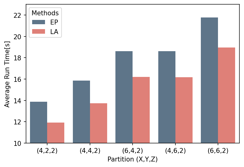
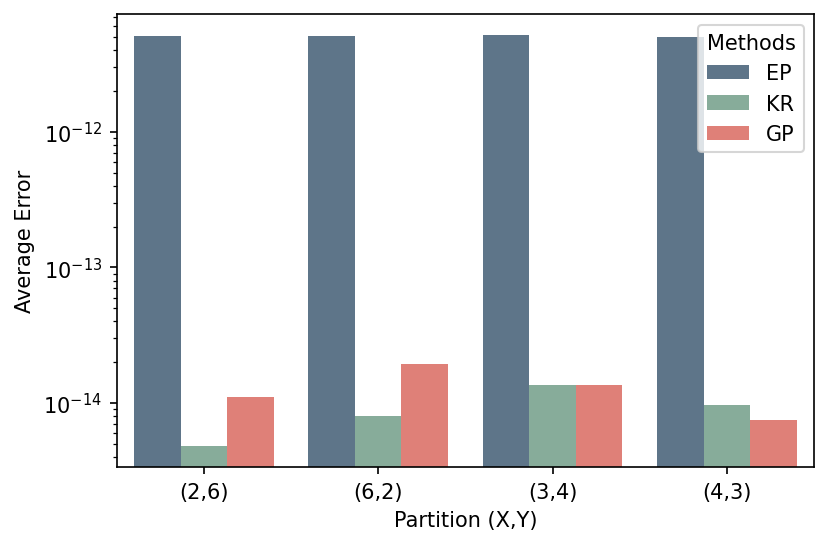
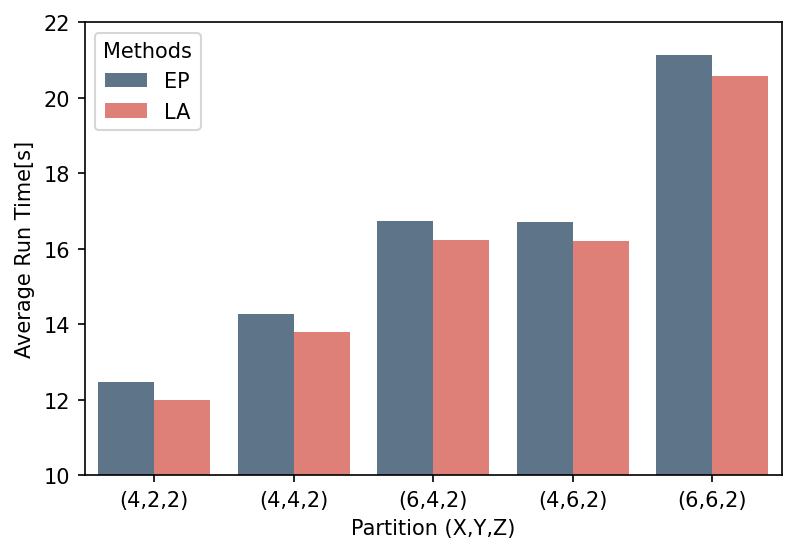
Figure 1: From left to right: i) run-time comparison for two 9600$\times$9600 matrices with minimum recovery threshold plus 7, ii) error comparison for 2-D codes, the plot is the logarithm of the error, and iii) run-time comparison for two 9600$\times$9600 matrices with the same number of workers. The second plot is log scaled because EP is numerically unstable.

IV Code Construction

IV-A Global Random Alloy Codes

If we let the uniformly random 2-product distribution be defined as

$$p^{*}(g^{i}_{j}=z)=\begin{cases}1-\sqrt{\frac{q-1}{q}}&\text{for }z=0\\ \frac{1}{\sqrt{q(q-1)}}&\text{for }z\neq 0\\ \end{cases},$$ (6)

and the uniformly random tensor distribution, or the uniformly random $l$-product tensor distribution, be defined as

$$p^{*}(g^{i}_{j}=z)=\begin{cases}1-\sqrt[l]{\frac{q-1}{q}}&\text{for }z=0\\ \frac{1}{\sqrt[l]{q(q-1)^{l-1}}}&\text{for }z\neq 0\\ \end{cases},$$ (7)

then we can define our random codes as

$$\tilde{A}_{k}=\sum_{i\in[x]}(g_{A})^{k}_{i}A_{i},\ \ \ \tilde{B}_{k}=\sum_{i\in[y]}(g_{B})^{k}_{i}B_{i},$$ (8)

for matrix multiplication and more generally as

$$(\tilde{A}_{1},...,\tilde{A}_{l})=\Bigg{(}\sum_{i\in[a_{1}]}(g_{A_{1}})^{k}_{i}A_{1,i},...,\sum_{i\in[x_{l}]}(g_{A_{l}})^{k}_{i}A_{l,i}\Bigg{)}.$$ (9)

The main intuition behind the construction of the codes is that we wish to define probability distributions for the coefficients of $g_{A}$ and $g_{B}$ in such a fashion that the resulting outer product code $g_{C}$ is i.i.d. uniformly randomly distributed. If one were to naively encode the coefficients of $g_{A}$ and $g_{B}$ using the uniformly random distribution, then the resulting code $g_{C}$ would be skewed towards 0. This is because 0 is not invertible and thus multiplication by zero does on form a permutation on $\mathbb{F}_{q}$. By slightly skewing $g_{A}$ and $g_{B}$ towards non-zero coefficients, we get that the resulting coefficients of the code $g_{C}$ is i.i.d. by the uniform random distribution. Because the decodability of the code only depends on the invertibility of $g_{C}$ the only important distribution is the resulting product distribution; Thm. 1 gives us that this is exactly the case.

Theorem 1 (Existence of Random Tensor codes for Matrix Multiplication).

There exists a probability distribution on $G_{A},G_{B}$ such that $G_{C}=G_{A}*G_{B}$ has it’s coefficients uniformly i.i.d; in particular, the probability of success for the $p$-adic scheme is $\prod_{i\in[1,k]}(1-q^{-i})>(1-q^{-1})^{k}$, where $k$ is the maximum rank of $G_{C}$.

Proof.

See Appx. -B for the proof. ∎

Lemma 2.

The codes given by Thm. 1 exist for all fields; in particular, we can extend the construction to all possible fields.

Proof.

See Appx. -C for the proof. ∎

Theorem 2 (Noisy Channel Coding Theorem for (2-D) Distributed Matrix Multiplication).

If $R=C-\epsilon$ and $z=1$, then random Alloy codes achieve the rate $R$ for large enough $x,y$. Conversely, if $R>C$, the probability of error cannot be made arbitrarily small for any tensor code.

Proof.

See Appx. -D for the proof. ∎

IV-B Locally Random Alloy Codes

The general local Random alloy code given by Alg. 1 is constructed locally by applying Eq. 9 to the outer products in a given efficient tensor decomposition for a tensor computation.

Algorithm 1 Locally_Random_Alloy_Codes

  Input: tensor $T$, decomposition $T_{1},...,T_{r}$, and vectors $A_{1},...,A_{l}$ where $T=T_{1}+...+T_{r}$, $T_{i}(A)=D_{i}(\mathcal{T}_{i}(E^{i}_{1}(A_{1}),...,E^{i}_{l}(A_{l})))$, the workers perform $\mathcal{T}_{t}$, and the $E^{i}_{j},D_{i}$ are low complexity tensors. workers $w^{t}_{k}$ indexed by $(t,k)$ where $t\in[r]$, $k\in[n/r]$.

  for $t\leq r$ do

     Master node generates $g^{t}:=(g_{A_{j}}^{t})^{k}_{i}$ according to Eq. 7

     Master computes $\widetilde{A}_{k,j}^{t}=\sum_{i\in[x_{j}]}(g_{A_{j}}^{t})^{k}_{i}E^{t}_{j}(A_{j,i})$

     Send worker $(t,k)$ the tasks $\widetilde{A}_{k,1}^{t},...,\widetilde{A}_{k,l}^{t}$

  end for

  Each worker $(t,k)$ computes $\mathcal{T}_{t}(\widetilde{A}_{k,1}^{t},...,\widetilde{A}_{k,l}^{t})$

  while Master has not received $\mathcal{R}^{t}$ tasks for each $t\in[r]$ do

     Master receives $\mathcal{T}_{t}(\widetilde{A}_{k}^{t})$ from next worker $(k,t)$

  end while

  for $t\leq r$ do

     Decode the $\mathcal{T}_{t}(\widetilde{A}_{k}^{t})$ by inverting $G_{C}^{t}$

  end for

  return  $(D_{i}T_{1}+...+D_{i}T_{r})(A_{1},...,A_{l})$

It is easier to understand it in the case where $T$ is the block matrix multiplication from Sec. I-A where the $\mathcal{T}$ that the workers perform is simply a smaller matrix multiplication. In this case we have that $E^{1}_{1}(A)={A}^{1}+{A}^{4}$ and $E^{1}_{2}(B)={B}^{1}+{B}^{4}$ and so on for $T_{2},...,T_{7}$. The $D_{i}$ are simply multiplication by $\pm 1$. In general, through a simple recursive argument, all fast matrix multiplications can be turned into such tensor decompositions.

Theorem 3 (Source Channel Separation Theorem for 3-D Distributed Matrix Multiplication).

If $R=\frac{p_{f}}{1-p_{f}}x^{3-\alpha}-\epsilon=\mathcal{O}(x^{2.687...})$, where $\alpha>0.31389$ is the bound for dual exponent of matrix multiplication given in [22], then local random alloy codes achieves the rate $R$ for large enough $x=y=z$ and $p_{f}\geq 1/2$. For the simpler case where $p_{f}<1/2$ one can replace $\frac{p_{f}}{1-p_{f}}$ with $2$.

Proof.

See Appx. -E for the proof. ∎

TABLE I: Comparison of Local Random Alloy (LRA) Codes with Entangled Polynomial (EP) Codes. $c$ is a constant and $x=y=z$ is the partition parameters. EC, CC, and DC are respectively the Encoding, Communication, and Decoding Complexity.

Code Scheme	EC	CC	DC	# Workers for $p_{f}\geq\frac{1}{2}$	# Workers for $p_{f}<\frac{1}{2}$
LRA	$\mathcal{O}(x^{2+2\alpha})$	$\mathcal{O}(x^{2+\alpha})$	$\mathcal{O}(x^{2+2\alpha})$	$\frac{p_{f}}{1-p_{f}}x^{3-\alpha}$	$2x^{3-\alpha}$
EP	$\mathcal{O}(x^{3}\log^{c}(x))$	$\mathcal{O}(x^{3})$	$\mathcal{O}(x^{3}\log^{c}(x))$	$\frac{p_{f}}{1-p_{f}}x^{3}$	$2x^{3}$

V Experimental Results

The experiments were performed on AWS EC2 Spot instances with a r5dn.xlarge for the master and c5n.large machines for the workers. AWS EC2 Spot instances are the most economical AWS cloud instances and are not necessarily guaranteed to have consistent or reliable performance, they are thus the best candidate (amongst Amazon’s provided choices) to test coded computing on actual non-simulated stragglers empirically. The experimental procedure was written using Mpi4py [46, 47], which is a python packaging providing python bindings for MPI. We compared our algorithm with Entangled Polynomial Codes and Khatari Rao Codes for the numerical stability experiments and simply with EP for the 3-D runtime experiments. For the runtime experiments we used (uniform and normal) randomly generated matrices of size 9600$\times$9600 for the runtime experiments and 1000 times the partition parameters $(x,y,z)$ for the numerical stability/error experiments; i.e., we performed experiments on size 6000$\times$2000 and 4000$\times$3000 for the error measurements. For the 3-D runtime experiments, we used networks of 22, 25, 36, 41, 50, 57, 71, 78, and 81 machines (including the master). For the 2-D numerical stability experiments, we used networks of size 7, 10, 13, 17, 21, 26 machines.

For a fair comparison with the EP codes, we ran two types of experiments: one with the same number of workers and one with the typical recovery threshold plus 7 workers. The numerical stability was tested by computing the relative error,

$$\frac{||(AB)_{\text{numpy}}-(AB)_{\mathcal{A}}||}{||(AB)_{\text{numpy}}||},$$

where $(AB)_{\text{numpy}}$ is the product $AB$ as numpy [48] computes it and $(AB)_{\mathcal{A}}$ is the is the product $AB$ as the algorithm $\mathcal{A}$ computes it. The numerical stability plot in Fig. 1 is given in logarithmic scale because the numerical instability of EP codes grows quite large for a large number of workers; however, random alloy codes also are more numerically stable than KR codes for some parameters.

Surprisingly, the results show that random alloy codes also performs faster than EP codes; this is surprising because theory only predicts performance improvement for asymptotic large partition parameters $(x,y,z)$. The performance gap remains true even after giving the random alloy codes the same number of workers as EP codes. The performance gap is slightly smaller in this case since now the master in the random alloy coding scheme must perform the same amount of encoding and send requests as the EP codes; however, the amount of messages received at the master and the decoding complexity is still unchanged and far smaller for random alloy codes in this case which allows random alloy codes to continue to perform better in this scenario as well.

VI Conclusion

We propose a novel framework for uniformly and effectively converting computationally efficient tensor rank decompositions into fault tolerant distributed coded algorithms. We gave proofs of asymptotic optimality for the case of matrix multiplication and gave empirical support that the proposed scheme performs better than many state of the art benchmarks for these computations. Nonetheless, there are still further research to be performed. A promising research direction is to explore the rate-distortion analogues of coded distributed tensor computations using this framework and rigorously proving the numerical stability of random alloy codes that we observed empirically. We gave a coding scheme for general tensors, i.e., Aq. 9 and Alg. 1; however, we did not prove the analogues of Thm. 1, Thm. 2, and Thm. 3 for more general tensors. The generalization of Thm. 1 is a straightforward generalization of a combinatorial argument but the generalizations of Thm. 2 and Thm. 3 are not clear, it is unlikely to be false. Likewise, generalizing to more general and decentralized topologies than the master-worker topology would be a natural extension. Finally, it would be interesting to explore what consequences the random nature of the code has for privacy and security. Since the resulting product of the codes $g_{C}$ is uniformly random it is reasonable to conjecture that the extension to secure multiparty computation is efficient and straightforward.

-A Proof of Lem. 1

Proof.

If we have a probability $p_{f}$ of having an erasure, then we have that

$$H(Y|X)=\sum_{x\in\mathcal{X}}p(x)H(Y|X=x)$$

$$=\sum_{x\in\mathcal{X}}p(x)H(p_{f})=H(p_{f})$$

$$=p_{f}\log\frac{1}{p_{f}}+(1-p_{f})\log\frac{1}{(1-p_{f})};$$

this follows from the the fact that given the knowledge that $X=(a_{1},a_{2})$ there are only two possibilities: either $Y=a_{1}a_{2}$ or $Y=E$ with probabilities $1-p_{f}$ and $p_{f}$ respectively.

Using the grouping property of entropy, i.e., that

we get that

$$H(\mathcal{Y})=H(p_{1},...,p_{|\mathcal{Y}|-1},p_{|\mathcal{Y}|})$$

$$=H(p_{1}+...+p_{|\mathcal{Y}|-1},p_{|\mathcal{Y}|})+\\ (p_{1}+...+p_{|\mathcal{Y}|-1})H(\frac{p_{1}}{p_{1}+...+p_{|\mathcal{Y}|-1}},...,\frac{p_{|\mathcal{Y}|-1}}{p_{1}+...+p_{|\mathcal{Y}|-1}}),$$

where $p_{|\mathcal{Y}|}=p_{f}$ and $p_{i}=$“ the probability of the $i^{th}$ element of $\mathcal{Y}\setminus\{E\}$”. But we have that $p_{1}+...+p_{|\mathcal{Y}|-1}=1-p_{f}$, which implies that $H(\mathcal{Y})=$

$$=H(p_{f})+(1-p_{f})H(Y\setminus\{E\}).$$

Finally, we get that

$$\begin{gathered}I(X,Y)=H(Y)-H(Y|X)\\ =H(p_{f})+(1-p_{f})H(Y\setminus\{E\})-H(p_{f})\\ =(1-p_{f})H(Y\setminus\{E\})=(1-p_{f})H(p_{1},...,p_{|\mathcal{Y}|-1}).\end{gathered}$$

Since we know that entropy is maximized when $p_{i}=p_{j}$ for all $i,j$, we conclude that

$$C=\max_{p\in\mathcal{D}(\mathcal{X})}I(X,Y)=(1-p_{f})\log(|\mathcal{Y}|-1).$$

∎

-B Proof of Thm. 1

Proof.

If we place the distribution $p^{*}$ from Eq. 6 on $G_{A},G_{B}$; then we get that

$$p((g_{C})^{k}_{i,j}=z)=\sum_{xy=z}p((g_{A})^{k}_{i}=x)p((g_{B})^{k}_{j}=y),$$

because $(g_{C})^{k}_{i,j}=(g_{C})^{k}_{i}(g_{C})^{k}_{j}$ and the distributions $p^{*}_{A},p^{*}_{B}$ are independent. Since $p^{*}_{A},p^{*}_{B}$ are also identically distributed we can set

$$u=p^{*}(g^{i}_{j}=0)=1-\sqrt{\frac{q-1}{q}}$$

$$(\forall z\neq 0)\ v=p^{*}(g^{i}_{j}=z)=\frac{1}{\sqrt{q(q-1)}}.$$

A simple combinatorial argument gives us that

$$p^{*}((g_{C})^{k}_{i,j}=z)=\begin{cases}u^{2}+2(q-1)uv&\text{for }z=0\\ (q-1)v^{2}&\text{for }z\neq 0\\ \end{cases},$$

i.e., there is: 1 way to get $x,y=0$, there are $2(q-1)$ ways to multiply some $x,y\neq 0$ with a zero to get a zero, and there are $q-1$ ways to get $x,y\neq 0$ to equal $z\neq 0$; these three cases correspond to the probabilities of $u^{2},uv,$ and $v^{2}$ respectively. Therefore, the probability of a 0 is equal to

$$p^{*}((g_{C})^{k}_{i,j}=0)=u^{2}+2(q-1)uv=$$

$\left(1-\sqrt{\frac{q-1}{q}}\right)^{2}+2(q-1)\left(1-\sqrt{\frac{q-1}{q}}\right)\left(\frac{1}{\sqrt{q(q-1)}}\right)=\frac{1}{q}$

Similarly, we have that

$$p^{*}((g_{C})^{k}_{i,j}=z)=(q-1)v^{2}=(q-1)\left(\frac{1}{\sqrt{q(q-1)}}\right)^{2}=\frac{1}{q},$$

for a non-zero $z$. Because $p^{*}((g_{C})^{k}_{i,j}=z)$ is a function of the values $p^{*}((g_{A})^{k}_{i}=0),...,p^{*}((g_{A})^{k}_{i}=q-1)$ and $p^{*}((g_{B})^{k}_{j}=0),...,p^{*}((g_{B})^{k}_{j}=q-1)$ we have that $k\neq k^{\prime}$ implies that $p^{*}((g_{C})^{k}_{i,j}=z)$ and $p^{*}((g_{C})^{k^{\prime}}_{i,j}=z)$ are independent. Therefore we have that any two rows of $G_{C}$ are independent Similarly if either $i\neq i^{\prime}$ or $j\neq j^{\prime}$ we have that $p^{*}((g_{C})^{k}_{i,j}=z)$ and $p^{*}((g_{C})^{k}_{i^{\prime},j^{\prime}}=z)$ are independent. Therefore we have independence of $G_{C}$ across columns.

The fact that the probability of a uniformly random matrix over a finite field has probability $\prod_{i\in[1,k]}(1-q^{-i})$ of having full rank is a standard counting exercise found in many combinatorics textbooks; e.g., Proposition 1.7.2 in [49]. ∎

-C Proof of Lem. 2

Proof.

There are two kinds of fields; there are those with characteristic $p$ and those with characteristic $0$. A classical theorem of Algebra states that those are all of the cases. If the field has characteristic $p$ then we are done, since it is also a classical theorem of algebra that any field, $\mathbb{F}$, that has $\mathrm{char}(\mathbb{F})=p$ and has $|\mathbb{F}|>p^{k}$, must have a copy of the field $\mathbb{F}_{q}$, as a sub-field, for all $q=p^{k^{\prime}}$ and $k^{\prime}\leq k$. Thus it remains to prove the theorem for $\mathrm{char}(\mathbb{F})=0$.

A classical theorem of linear algebra gives us that a square matrix has full rank if and only if the determinant of the matrix is non-zero. Furthermore, it is straightforward to prove that the determinant function,

$$\mathrm{det}(G)=\sum_{\sigma\in\mathcal{S}_{n}}(-1)^{\mathrm{sgn}(\sigma)}G_{0,\sigma(0)}\cdot...\cdot G_{n-1,\sigma(n-1)},$$

is, by virtue of its definition, a homomorphism. Similarly the function $\mathrm{mod}_{p}:\mathbb{Z}\rightarrow\mathbb{F}_{p}$ defined by $n\mapsto(n\mod p)$ is a well known homomorphism. If $G$ is a full rank matrix in $\mathbb{F}_{p}$ then when we consider the matrix $G$ as a matrix over $\mathbb{Z}$, call it $G_{\mathbb{Z}}$, we notice that the fact that $\mathrm{det}$ and $\mathrm{mod}_{p}$ and thus $\mathrm{det}\circ\mathrm{mod}_{p}$ are all homomorphisms gives us that

$$\mathrm{det}(G_{\mathbb{Z}})=0\implies\mathrm{det}(\mathrm{mod}_{p}(G_{\mathbb{Z}}))=0.$$

Therefore, if $G$ is full-rank, then $G_{\mathbb{Z}}$ is full rank. A classical theorem of algebra gives us that all fields with $\mathrm{char}(\mathbb{F})=0$ contain a copy of the integers, thus we exhausted all of the cases. ∎

-D Proof of Thm. 2

Proof.

(Achievability) If we fix an $\epsilon$ and generate product codes $\mathcal{C}=(G_{C},G_{A},G_{B})$ randomly according to the distribution in Eq. 6 and let

$$E_{1}=P(G_{C}\text{ fails})$$

and

$$E_{2}=P(\#\text{erasures}>r),$$

then we have that the probability of error is equal to

$$P(E_{f})=P(E_{1}\lor E_{2})\leq P(E_{1})+P(E_{2}).$$

If $S_{G}^{x,y}$ is the random variable corresponding to choosing a random $xy\times xy$ sub-matrix of $G_{C}$, then $S_{G}^{x,y}$ is also uniformly randomly distributed; furthermore, Thm. 1 gives us that

$$P(E_{1})=P(G_{C}\text{ fails})\leq P(\textrm{rank}(S_{G}^{xy})<xy)$$

since $P(\textrm{rank}(S_{G}^{xy})<xy)$ equals “the probability that the rows of $G_{C}$ corresponding to $\mathcal{W}$ will be a full rank matrix” for a fixed subset $\mathcal{W}=\{w_{1},...,w_{xy}\}$ of the workers. Therefore, Thm. 1 also gives us that $P(E_{1})\leq\prod_{i\leq xy}(1-q^{-i}).$

If we let

$$p^{G_{c}}_{e}(M_{1},M_{2})=P(E_{2}|M=(M_{1},M_{2}),\mathcal{C}=G_{C}),$$

then we have that

$$P(E_{2})\leq\sum_{G_{c}\in\mathfrak{C}}\sum_{(M_{1},M_{2})\in\mathcal{M}}p(E_{2},M_{1},M_{2},G_{c})$$

$$=\sum_{G_{c},M_{1},M_{2}}p^{G_{c}}_{e}(M_{1},M_{2})p(M_{1},M_{2},G_{C}).$$

For any fixed $M_{1},M_{2}$, and $G_{C}$ we have that

$$p^{G_{c}}_{e}(M_{1},M_{2})=P(Y^{n}\text{ has }>r\text{ erasures}).$$ (10)

For any fixed input $X=(M_{1},M_{2})$ we have that either $Y=M_{1}\cdot M_{2}$ or $Y=E$ with probabilities $1-p_{f}$ and $p_{f}$. Therefore, the probability of $Y=E$ or $Y\neq E$ (and by extension $Y^{n}$) is independent of any choice of $X=(M_{1},M_{2})$ or $\mathcal{C}=(G_{A},G_{B},G_{C})$ and Eq. 10 further gives us that $p^{G_{c}}_{e}(M_{1},M_{2})$ is also is independent of any choice of $X=(M_{1},M_{2})$ or $\mathcal{C}=(G_{A},G_{B},G_{C})$ as well. In particular, $M_{1},M_{2}$, and $G_{C}$ being fixed implies $Y^{n}$ is a Bernoulli process and the proof follows from the same argument for classical binary erasure channels by Lem. 1.

(Converse) Suppose for a contradiction that the capacity bound were violated by some product code $\mathcal{C}=(\mathcal{E},\mathcal{D})$, we will complete the proof by deriving a contradiction to the original Shannon theorem. Recall that the original definition of an error was

$$p^{\mathcal{C}}_{e}(M_{1},M_{2})=p(\mathcal{D}(Y^{n})\neq M_{1}M_{2}\ |\ X^{n}=\mathcal{E}(M_{1},M_{2})).$$

With this definition in mind, we define a new message set $\mathcal{N}$ as follows

$\mathcal{N}$ clearly defines a set of equivalence classes $[M_{1},M_{2}]_{\sim}$ corresponding to the equivalence relation

$$(M_{1},M_{2})\sim(M_{3},M_{4})\overset{def}{\iff}M_{1}M_{2}=M_{3}M_{4}.$$

Furthermore, it is also straightforward to see that $|\mathcal{N}|=|\mathcal{M}^{\prime}\setminus\mathcal{E}|$, i.e., it has as many elements as the output set, see Fig. 2.

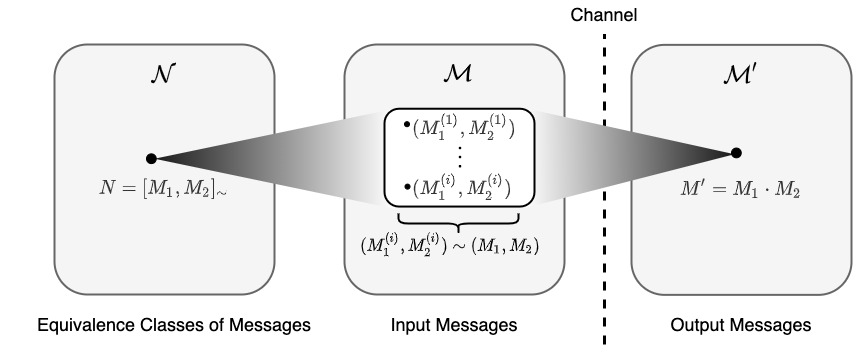
Figure 2: An illustration of the proof of the converse implication in Lem. 2. Two pair of matrices $(M^{(1)}_{1},M^{(1)}_{2})$ and $(M^{(i)}_{1},M^{(i)}_{2})$ are equivalent to one another if their respective products equal; i.e., if $M^{(1)}_{1}\cdot M^{(1)}_{2}=M^{(i)}_{1}\cdot M^{(i)}_{2}$. If the “messages” in $\mathcal{M}$ can be at a rate higher than the bound in Lem. 2 then the classical Shannon noisy is false.

For each equivalence class $[M_{1},M_{2}]_{\sim}$ pick a distinct representative. Suppose that we have a random variable $Z$ that takes values in the set $\mathcal{Z}$ and that $|\mathcal{Z}|=|\mathcal{N}|$. Since $|\mathcal{Z}|=|\mathcal{N}|$, there is a function $h:\mathcal{Z}\longrightarrow\mathcal{N}$ that is 1-1 and unto. If we let $j:\mathcal{N}\longrightarrow\mathcal{M}$ be the defined as

$$j:[M_{1},M_{2}]_{\sim}\mapsto(M_{1},M_{2}),$$

then the code

$$\mathcal{C}^{\prime}=(\mathcal{E}\circ j\circ h,h^{-1}\circ j^{-1}\circ\mathcal{D})$$

violates the classic Shannon theorem. This is because we defined the probability of error for a product code to be $p^{\mathcal{C}}_{e}(M_{1},M_{2})=p(\mathcal{D}(Y^{n})\neq M_{1}M_{2}\ |\ X^{n}=\mathcal{E}(M_{1},M_{2}))$. Therefore, if $h(z)=[M_{1},M_{2}]_{\sim}$, then we have that the classical definition of an error is equal to

$$\tilde{p}_{e}^{\mathcal{C}}(z)=p((h^{-1}j^{-1}\mathcal{D})(Y^{n})\neq z\ |\ X^{n}=(\mathcal{E}jh)(z))$$

$$=p((j^{-1}\mathcal{D})(Y^{n})\neq[M_{1},M_{2}]_{\sim}\ |\ X^{n}=(\mathcal{E}j)[M_{1},M_{2}]_{\sim})$$

$$=p(\mathcal{D}(Y^{n})\neq M_{1}M_{2}\ |\ X^{n}=\mathcal{E}(M_{1},M_{2}))=p^{\mathcal{C}}_{e}(M_{1},M_{2})$$

which contradicts the classical Shannon noisy channel theorem. ∎

-E Proof of Thm. 3

Proof.

Let $T=T_{1}+...+T_{r}$ be an optimal tensor rank decomposition for $(\frac{x}{\mu},y,z)=(\frac{z}{\mu},z,z)$ then we can apply the code in Eq. 8 to the $T_{i}$ to get $r$ optimal $(\mu,1,1)=(z^{1-\alpha},1,1)$ codes. Then this creates a block code for the larger $T$ via standard arguments by the method of strong types, i.e., Hoeffding’s inequality, as found in [50]. Taking approriate limits for the $\chi=(1+\lambda)\mu=(1+\lambda)z^{1-\alpha}$ as $x,y,z\to\infty$ using the Thm. 2 completes the proof; $\lambda$ is equal to the ratio of redundancy to original data needed asymptotically. The proof is completed if we can prove that $\lambda\to p_{f}^{-1}$ as $x,y,z\to\infty$.

To simplify the proof we prove it for a probability of failure $p=p_{f}\geq\frac{1}{2}$. If we give each worker group a factor of $\lambda$ extra workers and we want to know what is that probability that a percentage of $(p+\Delta)\%$ of them will fail, then we have that

$$P(\text{$(p+\Delta)\%$ of workers will fail})\leq\exp\left(-\frac{\Delta^{2}\chi}{2p\left(1-p\right)}\right)$$

by the Chernoff-Hoeffding inequality. We need $p+\Delta=\frac{\lambda z^{1-\alpha}}{(1+\lambda)z^{1-\alpha}}=\frac{\lambda}{1+\lambda}$ so that $\Delta=\frac{\lambda}{1+\lambda}-p.$ Therefore if we want the probability of the $z^{2}$ larger tasks $T_{1},...,T_{z^{2}}$ tasks (see [22] for a proof that $z^{2}$ rank-one tensors are needed for $(\frac{z}{\mu},z,z)$ size rectangular multiplication) to fail with less than $1-\epsilon$ probability the following bound

$$\left(1-\exp\left(-\frac{\left(\frac{\lambda}{1+\lambda}-p\right)^{2}\chi}{2p\left(1-p\right)}\right)\right)^{z^{2}}\geq 1-\epsilon,$$

is sufficient. Simple algebraic manipulation gives us that

$$z^{2}\ln\left(1-\exp\left(-\frac{\left(\frac{\lambda}{1+\lambda}-p\right)^{2}\chi}{2p\left(1-p\right)}\right)\right)\geq\ln\left(1-\epsilon\right).$$

But then $\exp\left(-\frac{\left(\frac{\lambda}{1+\lambda}-p\right)^{2}\chi}{2p\left(1-p\right)}\right)<1$ and the well known fact that $c<1\implies 1-c\geq\log(1-c)$ togehter imply that

$$z^{2}\left(1-\exp\left(-\frac{\left(\frac{\lambda}{1+\lambda}-p\right)^{2}\chi}{2p\left(1-p\right)}\right)\right)$$

$$\geq z^{2}\ln\left(1-\exp\left(-\frac{\left(\frac{\lambda}{1+\lambda}-p\right)^{2}\chi}{2p\left(1-p\right)}\right)\right)\geq\ln\left(1-\epsilon\right).$$

Simple algebraic manipulation gives us that

$$-\exp\left(-\frac{\left(\frac{\lambda}{1+\lambda}-p\right)^{2}\chi}{2p\left(1-p\right)}\right)\geq\frac{\ln\left(1-\epsilon\right)}{z^{2}}-1.$$

which in turn gives us $-\frac{\left(\frac{\lambda}{1+\lambda}-p\right)^{2}\chi}{2p\left(1-p\right)}\leq\ln\left(1-\frac{\ln\left(1-\epsilon\right)}{z^{2}}\right)$ and finally that

$$\frac{\lambda}{1+\lambda}\geq p+\sqrt{-\chi^{-1}2p\left(1-p\right)\ln\left(1-\frac{\ln\left(1-\epsilon\right)}{z^{2}}\right)}.$$

But fixing $p,\epsilon$ and letting $x,y,z,\chi\to\infty$ gives us that for any $\epsilon^{\prime}\to 0$, the inequality $\frac{\lambda}{1+\lambda}\geq p+\epsilon$ is satisfied. Thus we have that asymptotically we only need that $\frac{\lambda}{1+\lambda}\geq p$ which is equivalent to

$$\lambda\geq\frac{p_{f}}{1-p_{f}}$$

as was needed to show. ∎

References

- [1] T. J. Hastie, R. Tibshirani, and J. H. Friedman, “The elements of statistical learning,” in Springer Series in Statistics, 2009.
- [2] D. D. Lee and H. S. Seung, “Learning the parts of objects by non-negative matrix factorization,” Nature, vol. 401, pp. 788–791, 1999.
- [3] ——, “Algorithms for non-negative matrix factorization,” in NIPS, 2000.
- [4] H. Poon and P. M. Domingos, “Sum-product networks: A new deep architecture,” IEEE ICCV Workshops, pp. 689–690, 2011.
- [5] H. Hotelling, “Analysis of a complex of statistical variables into principal components.” 1933.
- [6] B. Schölkopf, A. J. Smola, and K.-R. Müller, “Nonlinear component analysis as a kernel eigenvalue problem,” Neural Computation, vol. 10, pp. 1299–1319, 1998.
- [7] P. Comon, “Independent component analysis, a new concept?” Signal Process., vol. 36, pp. 287–314, 1994.
- [8] S. J. Roberts and R. M. Everson, “Independent component analysis: Principles and practice,” 2001.
- [9] P. M. Kroonenberg and J. de Leeuw, “Principal component analysis of three-mode data by means of alternating least squares algorithms,” Psychometrika, vol. 45, pp. 69–97, 1980.
- [10] L. D. Lathauwer, B. D. Moor, and J. Vandewalle, “On the best rank-1 and rank-(r1 , r2, … , rn) approximation of higher-order tensors,” SIAM J. Matrix Anal. Appl., vol. 21, pp. 1324–1342, 2000.
- [11] ——, “A multilinear singular value decomposition,” SIAM J. Matrix Anal. Appl., vol. 21, pp. 1253–1278, 2000.
- [12] M. Vasilescu, “Multilinear independent component analysis,” 2004.
- [13] B. E. Boser, I. Guyon, and V. N. Vapnik, “A training algorithm for optimal margin classifiers,” in COLT ’92, 1992.
- [14] C. Cortes and V. Vapnik, “Support-vector networks,” Mach. Learn., vol. 20, pp. 273–297, 2004.
- [15] N. Cristianini and J. Shawe-Taylor, “An introduction to support vector machines and other kernel-based learning methods,” 2000.
- [16] M. A. Aizerman, “Theoretical foundations of the potential function method in pattern recognition,” 1964.
- [17] D. Haussler, “Convolution kernels on discrete structures,” 1999.
- [18] C. Watkins, “Kernels from matching operations,” 1999.
- [19] ——, “Dynamic alignment kernels,” 1999.
- [20] J. Shawe-Taylor and N. Cristianini, “Kernel methods for pattern analysis,” 2004.
- [21] Q. Yu, M. A. Maddah-Ali, and A. S. Avestimehr, “Straggler mitigation in distributed matrix multiplication: Fundamental limits and optimal coding,” ISIT, pp. 2022–2026, 2018.
- [22] F. L. Gall and F. Urrutia, Improved Rectangular Matrix Multiplication using Powers of the Coppersmith-Winograd Tensor, pp. 1029–1046.
- [23] T. G. Kolda and B. W. Bader, “Tensor decompositions and applications,” SIAM Review, vol. 51, pp. 455–500, 2009.
- [24] J. M. Landsberg, “Tensors: Geometry and applications,” 2011.
- [25] ——, “Geometry and complexity theory,” 2017.
- [26] K. Lee, M. Lam et al., “Speeding Up Distributed Machine Learning Using Codes,” IEEE Trans. Inf. Theory, pp. 1514–1529, 2018.
- [27] Q. Yu, M. A. Maddah-Ali, and A. S. Avestimehr, “Polynomial codes: an optimal design for high-dimensional coded matrix multiplication,” in NIPS, 2017.
- [28] S. Dutta, M. Fahim et al., “On the optimal recovery threshold of coded matrix multiplication,” IEEE Trans. Inf. Theory, pp. 278–301, 2020.
- [29] S. Dutta, Z. Bai et al., “A unified coded deep neural network training strategy based on generalized polydot codes,” ISIT, pp. 1585–1589, 2018.
- [30] K. Lee, C. Suh, and K. Ramchandran, “High-dimensional coded matrix multiplication,” in ISIT, 2017, pp. 2418–2422.
- [31] T. Baharav, K. Lee et al., “Straggler-proofing massive-scale distributed matrix multiplication with d-dimensional product codes,” in ISIT, 2018, pp. 1993–1997.
- [32] S. Wang, J. Liu, and N. Shroff, “Coded sparse matrix multiplication,” in ICML, 2018, pp. 5152–5160.
- [33] P. Soto, J. Li, and X. Fan, “Dual entangled polynomial code: Three-dimensional coding for distributed matrix multiplication,” in ICML, 2019.
- [34] S. Dutta, V. Cadambe, and P. Grover, ““short-dot”: Computing large linear transforms distributedly using coded short dot products,” IEEE Trans. Inf. Theory, pp. 6171–6193, 2019.
- [35] A. B. Das and A. Ramamoorthy, “Distributed matrix-vector multiplication: A convolutional coding approach,” in ISIT, 2019, pp. 3022–3026.
- [36] S. Hong, H. Yang et al., “Chebyshev polynomial codes: Task entanglement-based coding for distributed matrix multiplication,” in ICML, 2021, pp. 4319–4327.
- [37] Q. Yu, S. Li et al., “Lagrange coded computing: Optimal design for resiliency, security, and privacy,” in AISTATS, 2019, pp. 1215–1225.
- [38] Z. Jia and S. A. Jafar, “Generalized cross subspace alignment codes for coded distributed batch matrix multiplication,” in ICC, 2020, pp. 1–6.
- [39] P. Soto and J. Li, “Straggler-free coding for concurrent matrix multiplications,” in ISIT, 2020, pp. 233–238.
- [40] P. Soto, X. Fan et al., “Rook coding for batch matrix multiplication,” IEEE Trans. Commun., pp. 1–1, 2022.
- [41] R. G. L. D’Oliveira, S. E. Rouayheb, and D. A. Karpuk, “Gasp codes for secure distributed matrix multiplication,” ISIT, pp. 1107–1111, 2019.
- [42] L. Tang, K. Konstantinidis, and A. Ramamoorthy, “Erasure coding for distributed matrix multiplication for matrices with bounded entries,” IEEE Commun. Lett., vol. 23, pp. 8–11, 2019.
- [43] R. Tandon, Q. Lei et al., “Gradient coding: Avoiding stragglers in distributed learning,” in ICML, 2017, pp. 3368–3376.
- [44] P. J. Soto, I. Ilmer et al., “Lightweight projective derivative codes for compressed asynchronous gradient descent,” in ICML, 2022, pp. 20 444–20 458.
- [45] A. M. Subramaniam, A. Heidarzadeh, and K. R. Narayanan, “Random khatri-rao-product codes for numerically-stable distributed matrix multiplication,” Allerton, pp. 253–259, 2019.
- [46] L. Dalcín, R. Paz, and M. Storti, “Mpi for python,” J Parallel Distrib Comput., vol. 65, no. 9, pp. 1108–1115, 2005.
- [47] L. Dalcín, R. Paz et al., “Mpi for python: Performance improvements and mpi-2 extensions,” Journal of Parallel and Distributed Computing, vol. 68, no. 5, pp. 655–662, 2008.
- [48] C. R. Harris, K. J. Millman et al., “Array programming with NumPy,” Nature, vol. 585, no. 7825, pp. 357–362, Sep. 2020.
- [49] R. P. Stanley, “Enumerative combinatorics volume 1 second edition,” Cambridge studies in advanced mathematics, 2011.
- [50] I. Csiszár and J. Körner, “Information theory - coding theorems for discrete memoryless systems, second edition,” 1997.