Canonical and Non-canonical Inflation in the light of the recent BICEP/Keck results

Abstract

We discuss implications of the latest BICEP/Keck data release for inflationary models, with particular emphasis on scalar fields with non-canonical Lagrangians of the type ${\cal L}=X^{\alpha}-V(\phi)$. The observational upper bound on the tensor-to-scalar ratio, $r\leq 0.036$, implies that monotonically increasing convex potentials are now ruled out in the canonical framework. This includes the simplest classic inflationary potentials such as $\frac{1}{2}m^{2}\phi^{2}$ and $\lambda\phi^{4}$, as well as the whole family of monomial power law potentials $V(\phi)\sim\phi^{p}$. Instead, the current observations strongly favour asymptotically flat plateau potentials. However, working in the non-canonical framework, we demonstrate that the classic monomial potentials, as well as the Higgs potential with its Standard Model self-coupling, can easily be accommodated by the CMB data. Similarly we show that the inverse power law potential $V(\phi)\sim\phi^{-p}$, which leads to power law inflation in the non-canonical framework, also satisfies the latest CMB bounds. Significantly, $V(\phi)$ can originate from Planck scale initial values $V(\phi)\simeq\,m_{p}^{4}$ in non-canonical models while in plateau-like canonical inflation the initial value of the potential is strongly suppressed $V_{\rm plat}(\phi)\leq 10^{-10}\,m_{p}^{4}$. This has bearing on the issue of initial conditions for inflation and allows for the equipartition of the kinetic and potential terms in non-canonical models. Equipartition initial conditions can also be accommodated in simple extensions to plateau potentials such as the Margarita model of inflation which is discussed in this paper.

1 Introduction

The remarkable progress in Cosmology over the past three decades, reinforced by new theoretical insights and fostered by a plethora of precision cosmological missions, has resulted in the so-called ‘standard scenario’ of the universe in the form of the spatially flat $\Lambda$CDM model [1]. This model of ‘Concordance Cosmology’ successfully describes the evolution of our universe, both at the background as well as the perturbative level, commencing from almost a second after the hot Big Bang until the present epoch [2, 3] (however, see [4]). Nevertheless, the success of this standard model relies upon several (seemingly) unnatural initial conditions which include, at the background level: the spatial homogeneity, isotropy and near spatial flatness of the universe, and at the perturbative level: the existence of a spectrum of nearly scale-invariant adiabatic density fluctuations (which seed structure formation in the universe).

‘Cosmic Inflation’ has emerged as a leading prescription for describing the very early universe prior to the commencement of the radiative hot Big Bang phase [5, 6, 7, 8, 9, 10]. According to the inflationary paradigm, a transient epoch of at least 60-70 e-folds of rapid accelerated expansion suffices in setting natural initial conditions for cosmology in the form of spatial flatness as well as statistical homogeneity and isotropy on large angular scales [6, 7, 8, 11]. Of equal significance is the fact that cosmic inflation generates a spectrum of initial scalar fluctuations (via quantum fluctuations of a scalar degree of freedom) which later seed the formation of structure in the universe [12, 13, 14, 15, 11]. In addition to scalar perturbations, quantum fluctuations during inflation also create a spectrum of almost scale invariant tensor perturbations which later form gravity waves [16, 17].

The simplest models of inflation comprising of a single scalar field, called the ‘inflaton’, which is minimally coupled to gravity, make several distinct predictions [18], most of which have received spectacular observational confirmation, particularly from the latest CMB missions [19]. Current observational data lead to a scenario in which the inflaton $\phi$ slowly rolls down a shallow potential $V(\phi)$ thereby giving rise to a quasi-de Sitter early stage of near-exponential expansion.

As mentioned earlier, both scalar and tensor perturbations are generated during inflation. The latter constitute the relic gravitational wave background (GW) which imprints a distinct signature on the CMB power spectrum in the form of the B-mode polarization [19]. The amplitude of these relic GWs provides us information about the inflationary energy scale while their spectrum enables us to access general properties of the epoch of reheating, being exceedingly sensitive to the post-inflationary equation of state [17, 20]. The amplitude of inflationary tensor fluctuations, relative to that of scalar fluctuations, is usually characterised by the tensor-to-scalar ratio $r$. Different models of inflation predict different values of $r$ which is sensitive to the gradient of the inflaton potential $V^{\prime}(\phi)=\frac{dV(\phi)}{d\phi}$ relative to its height $V(\phi)$. Convex potentials predict large values for $r$, while concave potentials predict relatively small values of $r$. While the spectrum of inflationary tensor fluctuations has not yet been observed, current CMB observations are able to place an upper bound on the tensor-to-scalar ratio on large angular scales. In particular, the latest CMB observations of BICEP/Keck [21], combined with those of the PLANCK mission [19], place the strong upper bound $r\leq 0.036$ (at $95\%$ confidence). In this work we discuss the implications of this observational bound on single field inflationary models, with particular emphasis on scalar fields with a non-canonical Lagrangian density.

This most recent upper bound on $r$ has important consequences for single field canonical inflation. In particular, given $r\leq 0.036$, all monotonically increasing convex potentials, including the whole family of monomial potentials $V(\phi)\propto\phi^{p}$, are completely ruled out in the canonical framework. Among these strongly disfavoured models are the simplest classic inflaton potentials $\frac{1}{2}m^{2}\phi^{2}$ and $\lambda\phi^{4}$. Instead, the observational upper bound on $r$ appears to favour asymptotically flat potentials possessing one or two plateau-like wings; see [22].

Despite their excellent agreement with observations, plateau potentials may face some theoretical shortcomings [23]. It is sometimes felt that, being a theory of the very early universe, inflation should commence at the Planck scale with $\rho_{\phi}\sim m_{p}^{4}$. By contrast plateau potentials are extremely flat and imply $V(\phi)\leq 10^{-10}\,m_{p}^{4}$. Although a large value of the kinetic term $V(\phi)\ll{\dot{\phi}}^{2}\sim m_{p}^{4}$ can offset this difficulty, it implies that the universe cannot commence from equipartition initial conditions $V(\phi)\sim{\dot{\phi}}^{2}\sim m_{p}^{4}$. Moreover the small value of the inflaton potential, $V(\phi)\leq 10^{-10}\,m_{p}^{4}$, precludes the presence of a large curvature term, $|\rho_{K}|\sim m_{p}^{4}$, at the commencement of inflation. Indeed, since $\rho_{K}=-3\,m_{p}^{2}/a^{2}<0$ in a closed universe, an initial value $|\rho_{K}|\gg V(\phi)$ would imply that the universe would begin to contract prior to the onset of inflation in plateau potentials.

These issues can be successfully tackled in non-canonical models in which a small value of $r$ can be accommodated by changes to the non-canonical kinetic term. Thus small values of $r\leq 0.036$ can easily arise for convex potentials having the form $V(\phi)\propto\phi^{p}$ and $V(\phi)\propto\phi^{-p}$ [24, 25]. In particular, we shall show that the Standard Model (SM) Higgs field, which cannot source CMB-consistent inflation in the canonical framework (owing to its large self-coupling), can easily source inflation in the non-canonical framework. Consequently equipartition initial conditions can easily be accomodated in non-canonical inflationary models and in canonical models based on the Margarita potential.

Our paper is organised as follows: after a brief introduction of inflationary scalar field dynamics in section 2, we discuss inflation in the canonical framework in section 3 highlighting the implications of the latest CMB observations on plateau potentials. Section 4 demonstrates that some of the difficulties faced by plateau models can be circumvented in the Margarita family of potentials which interpolate between potentials which are convex at large $|\phi|$ and concave at moderate $|\phi|$. Inflation in the non-canonical framework is discussed in section 5. The concluding section 6 is dedicated to a discussion highlighting the major inferences drawn from this work.

We work in the units $c,\hbar=1$. The reduced Planck mass is defined to be $m_{p}\equiv 1/\sqrt{8\pi G}=2.43\times 10^{18}~{}{\rm GeV}$. We assume the background universe to be homogeneous and isotropic with the metric signature $(-,+,+,+)$.

2 Inflationary Dynamics

The action of a scalar field which couples minimally to gravity has the following general form

$$S[\phi]=\int{\rm d}^{4}x\,\sqrt{-g}\;{\cal L}(X,\phi)\,,$$ (2.1)

where the Lagrangian density ${\cal L}(\phi,X)$ is a function of the field $\phi$ and the kinetic term

$$X=\frac{1}{2}\partial_{\mu}\phi\;\partial^{\mu}\phi\,.$$ (2.2)

Varying (2.1) with respect to $\phi$ results in the equation of motion

$$\frac{\partial{\cal L}}{\partial\phi}-\left(\frac{1}{\sqrt{-g}}\right)\partial_{\mu}\left(\sqrt{-g}\frac{\partial{\cal L}}{\partial\left(\partial_{\mu}\phi\right)}\right)=0.$$ (2.3)

The energy-momentum tensor associated with the scalar field is

$$T^{\mu\nu}=\left(\frac{\partial{\cal L}}{\partial X}\right)\,\left(\partial^{\mu}\phi\;\partial^{\nu}\phi\right)-g^{\mu\nu}\,{\cal L}~{}.$$ (2.4)

Specializing to a spatially flat FRW universe and a homogeneous scalar field, one gets

$${\rm d}s^{2}=-{\rm d}t^{2}+a^{2}(t)\;\left[{\rm d}x^{2}+{\rm d}y^{2}+{\rm d}z^{2}\right]\,,$$ (2.5)

$$T^{\mu}_{\;\>\;\nu}=\mathrm{diag}\left(-\rho_{{}_{\phi}},p_{{}_{\phi}},p_{{}_{\phi}},p_{{}_{\phi}}\right),$$ (2.6)

where the energy density $\rho_{{}_{\phi}}$, and pressure $p_{{}_{\phi}}$, are given by

$$\rho_{{}_{\phi}} = \left(\frac{\partial{\cal L}}{\partial X}\right)\,(2\,X)-{\cal L},$$ (2.7)

$$p_{{}_{\phi}} = {\cal L},$$ (2.8)

and $X=-\frac{1}{2}\dot{\phi}^{2}$. The evolution of the scale factor $a(t)$ is governed by the Friedmann equations

$$\left(\frac{\dot{a}}{a}\right)^{2}\equiv H^{2}=\frac{1}{3m_{p}^{2}}\,\rho_{{}_{\phi}},$$ (2.9)

$$\frac{\ddot{a}}{a}\equiv\dot{H}+H^{2}=-\frac{1}{6m_{p}^{2}}\,\left(\rho_{{}_{\phi}}+3\,p_{{}_{\phi}}\right),$$ (2.10)

where $H\equiv\dot{a}/a$ is the Hubble parameter and $\rho_{{}_{\phi}}$ satisfies the conservation equation

$${\dot{\rho}_{{}_{\phi}}}=-3\,H\left(\rho_{{}_{\phi}}+p_{{}_{\phi}}\right)~{}.$$ (2.11)

3 Inflation in the Canonical Framework

In the standard inflationary paradigm, inflation is sourced by a single canonical scalar field $\phi$, with a suitable self-interaction potential $V(\phi)$, which is minimally coupled to gravity. For such a canonical scalar field

$${\cal L}(X,\phi)=-X-V(\phi)\,,$$ (3.1)

Substituting (3.1) into (2.7) and (2.8), we find

$$\rho_{{}_{\phi}} = \frac{1}{2}{\dot{\phi}}^{2}+\;V(\phi)\,,$$

$$p_{{}_{\phi}} = \frac{1}{2}{\dot{\phi}}^{2}-\;V(\phi)\,,~{}~{}$$ (3.2)

consequently the two Friedmann equations (2.9), (2.10) and the equation (2.11) become

$$H^{2}=\frac{1}{3m_{p}^{2}}\,\rho_{\phi}=\frac{1}{3m_{p}^{2}}\left[\frac{1}{2}{\dot{\phi}}^{2}+V(\phi)\right],$$ (3.3)

$$\dot{H}=\frac{\ddot{a}}{a}-H^{2}=-\frac{1}{2m_{p}^{2}}\,\dot{\phi}^{2},$$ (3.4)

$${\ddot{\phi}}+3\,H{\dot{\phi}}+V^{\prime}(\phi)=0~{}.$$ (3.5)

The extent of inflation is indicated by the total number of e-foldings of accelerated expansion

$$N_{e}\equiv\Delta N=N_{e}^{i}-N_{e}^{\rm end}=\log_{e}{\frac{a_{\rm end}}{a_{i}}}=\int_{t_{i}}^{t_{\rm end}}H(t)dt,$$ (3.6)

where $H(t)$ is the Hubble parameter during inflation. $N_{e}$ denotes the number of e-foldings before the end of inflation so that $N_{e}=N_{e}^{i}$ corresponds to the beginning of inflation while $N_{e}=N_{e}^{\rm end}=0$ corresponds to the end of inflation. $a_{i}$ and $a_{\rm end}$ denote the scale factor at the beginning and end of inflation respectively. Typically a period of quasi-de Sitter inflation lasting for at least 60-70 e-foldings is required in order to address the problems of the standard hot Big Bang model. We denote $N_{*}$ as the number of e-foldings (before the end of inflation) when the CMB pivot scale $k_{*}=(aH)_{*}=0.05~{}\rm Mpc^{-1}$ left the comoving Hubble radius during inflation. Typically $N_{*}\in[50,\,60]$ depending upon the details of reheating after inflation.

The quasi-de Sitter like phase corresponds to the inflaton field rolling slowly down the potential $V(\phi)$. This slow-roll regime of inflation, ensured by the presence of the Hubble friction term in equation (3.5), is usually characterised by the first two kinematical Hubble slow-roll parameters $\epsilon_{H}$, $\eta_{H}$, defined by [30, 11]

$$\epsilon_{H}=-\frac{\dot{H}}{H^{2}}=\frac{1}{2m_{p}^{2}}\,\frac{\dot{\phi}^{2}}{H^{2}}\,,$$ (3.7)

$$\eta_{H}=-\frac{\ddot{\phi}}{H\dot{\phi}}=\epsilon_{H}+\frac{1}{2\epsilon_{H}}\,\frac{d\epsilon_{H}}{dN_{e}}\,,$$ (3.8)

where the slow-roll regime of inflation corresponds to

$$\epsilon_{H},~{}\eta_{H}\ll 1\,.$$ (3.9)

The slow-roll regime is also often characterised by the dynamical potential slow-roll parameters [11], defined by

$$\epsilon_{{}_{V}}=\frac{m_{p}^{2}}{2}\left(\frac{V^{\prime}}{V}\right)^{2}\,,~{}~{}\eta_{{}_{V}}=m_{p}^{2}\,\left(\frac{V^{\prime\prime}}{V}\right)\,.$$ (3.10)

For small values of these parameters $\epsilon_{H}\ll 1,\,\eta_{H}\ll 1$, one finds $\epsilon_{H}\simeq\epsilon_{{}_{V}}$ and $\eta_{H}\simeq\eta_{{}_{V}}-\epsilon_{{}_{V}}$. Using the definition of Hubble parameter, $H=\dot{a}/a$, we have $\ddot{a}/a=\dot{H}+H^{2}=H^{2}(1+\dot{H}/H^{2})$. From the expression for $\epsilon_{H}$ in (3.7), it is easy to see that

$$\frac{\ddot{a}}{a}=\big{(}1-\epsilon_{H}\big{)}\,H^{2}~{}.$$ (3.11)

Which implies that the universe accelerates, ${\ddot{a}}>0$, when $\epsilon_{H}<1$. Using equation (3.3), the expression for $\epsilon_{H}$ in (3.7) reduces to $\epsilon_{H}\simeq\frac{3}{2}\frac{\dot{\phi}^{2}}{V}$ when ${\dot{\phi}}^{2}\ll V$. In fact, under the slow-roll conditions (3.9), the Friedmann equations (3.3) and (3.5) take the form

$$H^{2}\simeq\frac{1}{3m_{p}^{2}}V(\phi)\,,$$ (3.12)

$$\dot{\phi}\simeq-\frac{V^{\prime}(\phi)}{3H}\,.$$ (3.13)

Quantum fluctuations

In the standard scenario of a minimally coupled single canonical scalar field $\phi$ as the inflaton, two gauge independent massless fields, one scalar and one transverse traceless tensor, get excited during inflation and receive quantum fluctuations that are correlated over super-Hubble scales [31] at late times. The evolution of the scalar degree of freedom, called the comoving curvature perturbation $\cal R$ is described by the following second order action [11]

$$S_{(2)}\left[\cal R\right]=\frac{1}{2}\int{\rm d}^{4}x~{}a^{3}\frac{\dot{\phi}^{2}}{H^{2}}\left[\dot{\cal R}^{2}-\frac{1}{a^{2}}\left(\partial_{i}\cal R\right)^{2}\right]~{},$$ (3.14)

which upon the change of variable

$$v\equiv z{\cal R}~{},\quad\mbox{with}\quad z=am_{p}\sqrt{2\epsilon_{H}}=a\,\frac{\dot{\phi}}{H}\,,$$ (3.15)

takes the form

$$S_{(2)}\left[v\right]=\frac{1}{2}\int{\rm d}^{4}x\left[\left(v^{\prime}\right)^{2}-\left(\partial_{i}v\right)^{2}+\frac{z^{\prime\prime}}{z}v^{2}\right]~{},$$ (3.16)

where $(^{\prime})$ denotes the derivative with respect to the conformal time $\tau=\int\frac{dt}{a(t)}$. The variable $v$, which itself is a scalar quantum field like $\cal R$, is called the Mukhanov-Sasaki variable in literature. Its Fourier modes $v_{k}$ satisfy the Mukhanov-Sasaki equation [32, 33]

$$v^{\prime\prime}_{k}+\left(k^{2}-\frac{z^{\prime\prime}}{z}\right)v_{k}=0~{},$$ (3.17)

where the effective mass term is given by the following exact expression [34]

$$\frac{z^{\prime\prime}}{z}=a^{2}H^{2}\left(2-\epsilon_{1}+\frac{3}{2}\epsilon_{2}+\frac{1}{4}\epsilon_{2}^{2}-\frac{1}{2}\epsilon_{1}\epsilon_{2}+\frac{1}{2}\epsilon_{2}\epsilon_{3}\right)~{},$$ (3.18)

with $\epsilon_{1}=\epsilon_{H}$ and

$$\epsilon_{n+1}=-\frac{d\ln{\epsilon_{n}}}{dN_{e}}~{}$$ (3.19)

are the ‘Hubble flow’ parameters. Given a mode $k$, at sufficiently early times when it is sub-Hubble i.e $k\gg aH$, we can assume $v$ to be in the Bunch-Davies vacuum [35] satisfying

$$v_{k}\rightarrow\frac{1}{\sqrt{2k}}e^{-ik\tau}~{}.$$ (3.20)

During inflation as the comoving Hubble radius falls (see figure 1), this mode starts becoming super-Hubble i.e $k\ll aH$ and equation (3.17) dictates that $|v_{k}|/z$ approaches a constant value. By solving the Mukhanov-Sasaki equation we can estimate the dimensionless primordial power-spectrum of $\cal R$ using the following relation [31]

$$P_{\cal R}\equiv\frac{k^{3}}{2\pi^{2}}\,|{\cal R}_{k}|^{2}\Big{|}_{k\ll aH}=\frac{k^{3}}{2\pi^{2}}\,\frac{|v_{k}|^{2}}{z^{2}}\Big{|}_{k\ll aH}~{}.$$ (3.21)

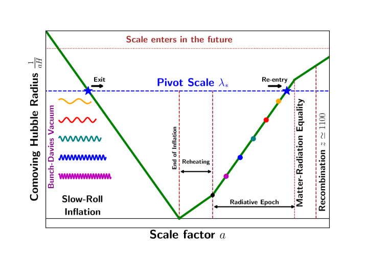
Figure 1: This figure schematically illustrates the evolution of the comoving Hubble radius $(aH)^{-1}$ with scale factor, both plotted in the logarithmic scale. During inflation $(aH)^{-1}$ decreases which causes physical scales to exit the Hubble radius. After inflation ends $(aH)^{-1}$ increases, and physical scales begin to re-enter the Hubble radius. The CMB pivot scale, as used by the Planck mission, is set at $k_{*}=0.05~{}{\rm Mpc}^{-1}$ and has been depicted by the dashed blue line. Note that $(aH)^{-1}\propto a$ during the radiative regime and $(aH)^{-1}\propto a^{-1}$ during inflation.

During slow-roll inflation, the factor $\frac{z^{\prime\prime}}{z}=\frac{\nu^{2}-0.25}{\tau^{2}}$ with $\nu\approx 1.5+\epsilon_{H}+\frac{\dot{\epsilon}_{H}}{2H\epsilon_{H}}$. The solution to the Mukhanov-Sasaki equation with suitable Bunch-Davies vacuum conditions can be written in terms of Hankel functions of second kind $H^{(2)}_{\nu}$ and the subsequent computation of the power spectrum of $\cal R$ leads to the famous slow-roll approximation formula [11]

$$P_{\cal R}=\frac{1}{8\pi^{2}}\left(\frac{H}{m_{p}}\right)^{2}\frac{1}{\epsilon_{H}}~{}.$$ (3.22)

On large cosmological scales which are accessible to CMB observations, the scalar power spectrum typically takes the form of a power law represented by

$$P_{\cal R}(k)=A_{{}_{S}}\left(\frac{k}{k_{*}}\right)^{n_{{}_{S}}-1},$$ (3.23)

where $A_{{}_{S}}=P_{\cal R}(k_{*})$ is the amplitude of the scalar power spectrum at the pivot scale $k=k_{*}$,

$$A_{{}_{S}}=\frac{1}{8\pi^{2}}\left(\frac{H}{m_{p}}\right)^{2}\frac{1}{\epsilon_{H}}\bigg{|}_{k=k_{*}}~{}.$$ (3.24)

The scalar spectral tilt $n_{{}_{S}}$, in the slow-roll regime is given by [11]

$$n_{{}_{S}}-1\equiv\frac{d\,\mathrm{ln}P_{\cal R}}{d\,\mathrm{ln}k}=2\eta_{H}-4\epsilon_{H}~{}.$$ (3.25)

Similarly the tensor power spectrum, in the slow-roll limit, is represented by

$$P_{T}(k)=A_{{}_{T}}\left(\frac{k}{k_{*}}\right)^{n_{{}_{T}}},$$ (3.26)

with the amplitude of tensor power spectrum at the CMB pivot scale is given by [11, 31]

$$A_{{}_{T}}\equiv P_{T}(k_{*})=\frac{2}{\pi^{2}}\left(\frac{H}{m_{p}}\right)^{2}\bigg{|}_{k=k_{*}}~{},$$ (3.27)

and the tensor spectral index (with negligible running) is given by

$$n_{{}_{T}}=-2\,\epsilon_{H}~{}.$$ (3.28)

The tensor-to-scalar ratio $r$ is defined by

$$r\equiv\frac{A_{{}_{T}}}{A_{{}_{S}}}=16\,\epsilon_{H}~{},$$ (3.29)

yielding the single field consistency relation

$$r=-8\,n_{{}_{T}}~{}.$$ (3.30)

We therefore find that the the slow-roll parameters $\epsilon_{H}$ and $\eta_{H}$ play a key role in characterising the power spectra of scalar and tensor fluctuations during inflation. In the next section, we discuss the implications of the latest CMB observations for the slow-roll parameters and for other relevant inflationary observables. In order to relate the CMB observables to the inflaton potential $V(\phi)$, we work with the potential slow-roll parameters defined in equation (3.10).

3.1 Implications of the latest CMB observations for canonical inflation

Consider a canonical scalar field minimally coupled to gravity and having the potential

$$V(\phi)=V_{0}\,f\left(\frac{\phi}{m_{p}}\right)~{}.$$ (3.31)

The potential slow-roll parameters (3.10) are given by

$$\epsilon_{{}_{V}}=\frac{m_{p}^{2}}{2}\left(\frac{f^{\prime}}{f}\right)^{2}~{},$$ (3.32)

$$\eta_{{}_{V}}=m_{p}^{2}\left(\frac{f^{\prime\prime}}{f}\right)~{}.$$ (3.33)

In the slow-roll limit $\epsilon_{{}_{V}},\,\eta_{{}_{V}}\ll 1$, the scalar power spectrum is given by the expression (3.23) with the amplitude of scalar power at the CMB pivot scale $k\equiv k_{*}=0.05~{}{\rm Mpc}^{-1}$ expressed as [11]

$$A_{{}_{S}}\equiv P_{\cal R}(k_{*})\simeq\frac{1}{24\pi^{2}}\frac{V_{0}}{m_{p}^{4}}\frac{f\left(\phi_{k}\right)}{\epsilon_{{}_{V}}(\phi_{k})}\bigg{|}_{k=k_{*}}~{},$$ (3.34)

and the scalar spectral index (with negligible running) is given by

$$n_{{}_{S}}\simeq 1+2\,\eta_{{}_{V}}(\phi_{*})-6\,\epsilon_{{}_{V}}(\phi_{*})~{},$$ (3.35)

where $\phi_{*}$ is the value of the inflaton field at the Hubble exit of CMB pivot scale $k_{*}$. Similarly the amplitude of tensor power spectrum at the CMB pivot scale is given by

$$A_{{}_{T}}\equiv P_{T}(k_{*})=\frac{2}{\pi^{2}}\left(\frac{H_{k}^{\rm inf}}{m_{p}}\right)^{2}\bigg{|}_{k=k_{*}}\simeq\frac{2}{3\pi^{2}}\frac{V_{0}}{m_{p}^{4}}f\left(\phi_{k}\right)\bigg{|}_{k=k_{*}}~{},$$ (3.36)

where $H_{k}^{\rm inf}$ is the Hubble parameter during the Hubble exit of mode k. The tensor spectral index (3.28) becomes

$$n_{{}_{T}}\simeq-2\,\epsilon_{{}_{V}}(\phi_{*})~{},$$ (3.37)

and the tensor-to-scalar ratio (3.29) can be written as

$$r\simeq 16\,\epsilon_{{}_{V}}(\phi_{*})~{},$$ (3.38)

satisfying the single field consistency relation (3.30). From the CMB observations of Planck 2018 [19], we have

$$A_{{}_{S}}=2.1\times 10^{-9}~{},$$ (3.39)

while the $2\sigma$ constraint on the scalar spectral index is given by

$$n_{{}_{S}}\in[0.957,0.976]~{}.$$ (3.40)

Similarly the constraint on the tensor-to-scalar ratio $r$, from the latest combined observations of Planck 2018 [19] and BICEP/Keck [21], is given by

$$r\leq 0.036~{},$$ (3.41)

which translates into $A_{{}_{T}}\leq 3.6\times 10^{-2}\,A_{{}_{S}}$. Equation (3.36) helps place the following upper bound on the inflationary Hubble scale $H_{k}^{\rm inf}$ and the energy scale during inflation $E_{\inf}$

$$H_{k}^{\rm inf}\leq 4.7\times 10^{13}~{}{\rm GeV}~{},$$ (3.42)

$$E_{\inf}\equiv\left[\sqrt{3}\,m_{p}\,H_{k}^{\rm inf}\right]^{1/2}\leq 1.4\times 10^{16}~{}{\rm GeV}~{}~{}.$$ (3.43)

Similarly the CMB bound on $r$ when combined with (3.38) translates into an upper bound on the first slow-roll parameter

$$\epsilon_{H}\simeq\epsilon_{{}_{V}}\leq 0.00225~{},$$ (3.44)

rendering the tensor tilt from equation (3.37) to be negligibly small

$$|n_{{}_{T}}|\leq 0.0045~{}.$$ (3.45)

Given the upper limit on $\epsilon_{{}_{V}}$, using the CMB bound on $n_{{}_{S}}$ from (3.40) in (3.35), we infer that the second slow-roll parameter is negative and obtain interesting upper and lower limits on its magnitude, given by

$$|\eta_{H}|\in[0.0075,0.0215]~{}.$$ (3.46)

The EOS $w_{\phi}$ of the inflaton field is given by

$$w_{\phi}=\frac{\frac{1}{2}\dot{\phi}^{2}-V(\phi)}{\frac{1}{2}\dot{\phi}^{2}+V(\phi)}\simeq-1+\frac{2}{3}\epsilon_{{}_{V}}(\phi)\,,$$ (3.47)

Therefore one finds from (3.44) the following constraint on the inflationary EOS at the pivot scale

$$w_{\phi}\leq-0.9985\,,$$ (3.48)

implying that the expansion of the universe during inflation was near exponential (quasi-de Sitter like).

Given the latest CMB constraints on $n_{{}_{S}}$ and especially the upper bound on the tensor-to-scalar ratio $r$ in (3.41), a number of famous models of inflation are strongly disfavoured. These include the simplest quadratic chaotic potential $\frac{1}{2}m^{2}\phi^{2}$, along with other monotonically increasing convex potentials, see figure 2. It is important to stress that the entire family of power law potentials $V(\phi)\propto\phi^{p}$ are now observationally ruled out as shown by the lime colour stripe in figure 2.

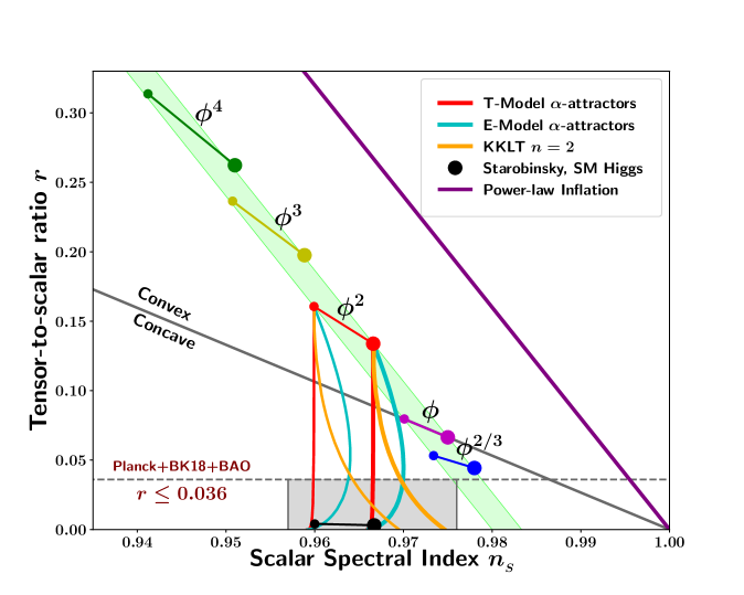
Figure 2: This figure plots the tensor-to-scalar ratio $r$ versus the scalar spectral index $n_{{}_{S}}$ for a number of inflationary potentials (the thinner and thicker dots and curves correspond to $N_{*}=50,\,60$ respectively). These include predictions of plateau potentials such as the Starobinsky model, the Standard Model Higgs inflation, the T-model and E-model $\alpha$-attractors as well as the KKLT inflation. The CMB 2$\sigma$ bound $0.957\leq n_{{}_{S}}\leq 0.976$ and the upper bound on the tensor-to-scalar ratio $r\leq 0.036$ are indicated by the shaded grey colour region. Given the upper bound on $r$, it is easy to see that observations favour concave potentials over convex ones.

Indeed, CMB observations now favour potentials exhibiting asymptotically flat plateau-like wings. In the literature of inflationary model building [36], there exist a number of plateau potentials that satisfy the CMB constraints. These include single parameter potentials such as the Starobinsky model [5, 37, 26], and the non-minimally coupled Standard Model (SM) Higgs inflation [27, 28, 26], along with a number of important plateau potentials with two parameters, such as the T-model and E-model $\alpha$-attractors [38, 39], and the D-brane KKLT potential [40, 41, 42, 22].

3.2 Important plateau potentials as future CMB targets

An asymptotically flat potential has the general functional form

$$V(\phi)=V_{0}\,f\left(\lambda\frac{\phi}{m_{p}}\right)~{},$$ (3.49)

such that $V(\phi)\longrightarrow V_{0}$ at large field values $\lambda\phi\gg m_{p}$. Such a potential, schematically represented in figure 3, usually features one or two plateau-like wings for large field values away from the minimum of the potential, depending upon whether the potential is asymmetric or symmetric. Below we discuss a number of important plateau potentials in light of the latest CMB observations.

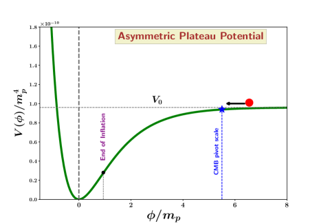
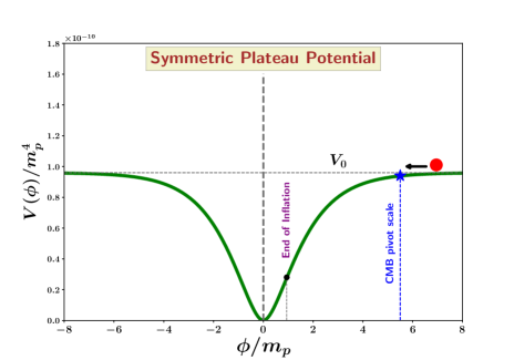
Figure 3: This figure schematically depicts asymptotically flat inflationary plateau potentials. The left panel shows an asymmetric potential featuring only a single plateau-like wing which supports slow-roll inflation. While the right panel shows a symmetric potential possessing two plateau-like wings, both of which can support slow-roll inflation.

1. Starobinsky model

   The potential for Starobinsky inflation [5] in the Einstein frame, in which the scalaron takes the form of a canonical scalar field minimally coupled to gravity, is given by [37, 26]

   $$V(\phi)=V_{0}\,\left(1-e^{-\frac{2}{\sqrt{6}}\frac{\phi}{m_{p}}}\right)^{2}~{}.$$ (3.50)

   This potential features a single parameter $V_{0}$, which is related to the scalaron mass $m$ by $V_{0}=\frac{3}{4}m^{2}m_{p}^{2}$ [26], and whose value is completely fixed by the CMB normalization (3.39). The prediction of $\{n_{{}_{S}},r\}$ for the Starobinsky potential is given by

   $$n_{{}_{S}}\simeq 1-\frac{2}{N_{*}}\,,~{}~{}r\simeq\frac{12}{N_{*}^{2}}\,,~{}{\rm for}~{}N_{*}\gg 1\,,$$ (3.51)

   which is shown by black colour dots in figure 2. As per standard convention, the smaller and larger black dots represent $\{n_{{}_{S}},r\}$ predictions of Starobinsky potential corresponding to $N_{*}=50,\,60$ respectively. It is important to note that the predictions of Starobinsky inflation lie at the centre of the observationally allowed region of $\{n_{{}_{S}},r\}$ (shown in grey in fig. 2), making it one of the most favourable inflationary models at present.

2. Non-minimally coupled Standard Model (SM) Higgs inflation

   The SM Higgs inflation was originally formulated [27, 28] in the Jordan frame where the Higgs field is non-minimally coupled to the scalar (Ricci) curvature of space-time. One can however transform it to the Einstein frame by a conformal transformation of the metric [26, 28] so that the Einstein frame action describes a canonical scalar field minimally coupled to gravity. The corresponding SM Higgs inflaton potential, for large field values, takes the form

   $$V(\phi)\simeq V_{0}\,\left(1-e^{-\frac{2}{\sqrt{6}}\frac{|\phi|}{m_{p}}}\right)^{2}~{}.$$ (3.52)

   The above potential also features a single parameter $V_{0}$, which is related to the strength of the non-minimal coupling $\xi$ by $V_{0}=\frac{\lambda m_{p}^{4}}{4\xi^{2}}$ as shown in [28, 26], where $\lambda=0.1$ is the SM Higgs self-coupling. Its value is completely fixed by the CMB normalization (3.39). Given the similarity in the functional form of (3.50) and (3.52), the prediction of the non-minimally coupled SM Higgs inflation for $\{n_{{}_{S}},r\}$ is similar to that of Starobinsky inflation, given by (3.51).

3. T-model $\alpha$-attractor

   The T-model $\alpha$-attractor potential [22] is a symmetric plateau potential of the functional form

   $$V(\phi)=V_{0}\,\tanh^{2q}{\left(\lambda\frac{\phi}{m_{p}}\right)}\,,~{}~{}2q=p>0~{}.$$ (3.53)

   For a given value of $p$, the T-model potential has two parameters, namely $V_{0}$ and $\lambda$. As usual, the value of $V_{0}$ is fixed by the CMB normalization (3.39) while $\lambda$ determines the predicted value of $\{n_{{}_{S}},r\}$ for this potential.

   

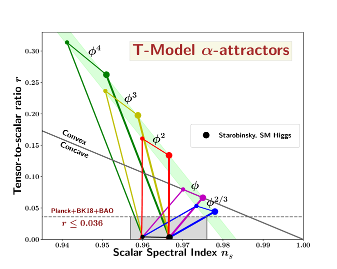
   Figure 4: This figure is a plot of the tensor-to-scalar ratio $r$, versus the scalar spectral index $n_{{}_{S}}$, for the T-model $\alpha$-attractor (3.53) (the thinner and thicker curves correspond to $N_{*}=50,\,60$ respectively). The latest CMB 2$\sigma$ bound $0.957\leq n_{{}_{S}}\leq 0.976$ and the upper bound on the tensor-to-scalar ratio $r\leq 0.036$ are indicated by the shaded grey colour region. It is important to note that upon increasing the value of $\lambda$, the predictions of T-model potential (3.53) for different values of $p$ converge towards the cosmological attractor at the centre, described by equation (3.54).

   Predictions of the simplest T-model potential, which corresponds to $p=2$ in equation (3.53), are shown by the red colour curves in figure 2. As we vary value of $\lambda$ from $\lambda:0\longrightarrow\infty$, the $r$ vs $n_{{}_{S}}$ values trace out continuous curves in figure 2 (the thinner and thicker red curves correspond to $N_{*}=50,\,60$ respectively). We notice that in one limit, namely $\lambda\ll 1$, the CMB predictions for $\{n_{{}_{S}},r\}$ of the T-model matches with that of the quadratic $\phi^{2}$ potential owing to the fact that the potential (3.53) for $p=2$ behaves like $V(\phi)\propto\phi^{2}$ for $\lambda\phi\ll m_{p}$. In fact this is true in general for the T-model potential with any value of $p$ in (3.53), leading to the behaviour $V(\phi)\propto\phi^{p}$ for $\lambda\phi\ll m_{p}$, which is demonstrated in figure 4. However in the opposite limit, namely $\lambda\geq 1$ (which results in $\exp{\left(\lambda\phi_{*}/m_{p}\right)}\gg 1$), the predictions of T-model become [22]

   $$n_{{}_{S}}\simeq 1-\frac{2}{N_{*}}\,,~{}~{}r\simeq\frac{2}{\lambda^{2}N_{*}^{2}}\,,~{}{\rm for}~{}N_{*}\gg 1\,,$$ (3.54)

   which is independent of $p$ (see [20]). Due to this property these models are called ‘cosmological attractors’ in [22].

4. E-model $\alpha$-attractor

   The E-model $\alpha$-attractor potential [22] is an asymmetric plateau potential of the functional form

   $$V(\phi)=V_{0}\,\left(1-e^{-\lambda\frac{\phi}{m_{p}}}\right)^{2q}\,,~{}~{}~{}2q=p>0\,.$$ (3.55)

   For $p=2$ and $\lambda=2/\sqrt{6}$, the E-model potential coincides with Starobinsky potential. In the limit $\lambda\geq 1$ (which results in $\exp{\left(\lambda\phi_{*}/m_{p}\right)}\gg 1$), the predictions of E-model become [22]

   $$n_{{}_{S}}\simeq 1-\frac{2}{N_{*}}\,,~{}~{}r\simeq\frac{8}{\lambda^{2}N_{*}^{2}}\,,~{}{\rm for}~{}N_{*}\gg 1\,,$$ (3.56)

   which again is independent of $p$ (see [20]). The CMB predictions $\{n_{{}_{S}},r\}$ of E-model potential are shown by the cyan colour curves in figure 2 for the case $p=2$. (the thinner and thicker cyan curves correspond to $N_{*}=50,\,60$ respectively).

5. D-brane KKLT potential

   The D-brane KKLT inflation [40, 41] potential has the following general form [42, 22]

   $$V(\phi)=V_{0}\,\frac{\phi^{n}}{\phi^{n}+M^{n}}\,,$$ (3.57)

   where $M$ is a fundamental scale of the theory. This is a symmetric plateau potential, like the T-model $\alpha$-attractor (3.53). However the KKLT potential approaches plateau behaviour (saturates) algebraically, in contrast to the exponential approach to plateau behaviour exhibited by the T-model potential.

   

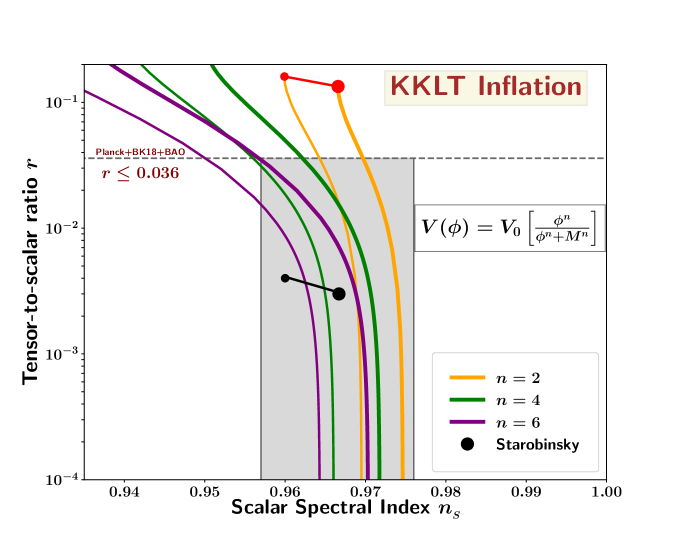
   Figure 5: This figure is a plot of the tensor-to-scalar ratio $r$ versus the scalar spectral index $n_{{}_{S}}$ for KKLT inflation (3.57) (the thinner and thicker curves correspond to $N_{*}=50,\,60$ respectively). The latest CMB 2$\sigma$ bound $0.957\leq n_{{}_{S}}\leq 0.976$ and the upper bound on the tensor-to-scalar ratio $r\leq 0.036$ are indicated by the shaded grey colour region.

   In the limit $M\gg m_{p}$, the potential asymptotes to a monomial power law form $V(\phi)\propto\phi^{n}$, the predictions of which are strongly disfavoured by observations. In the opposite limit, namely $M\ll m_{p}$, the potential is plateau-like, $V(\phi)\longrightarrow V_{0}$, whose predictions satisfy the CMB data very well. Figure 5 shows the $r$ vs $n_{{}_{S}}$ plot for KKLT potential (3.57) for three different values of $n$ (the thinner and thicker curves correspond to $N_{*}=50,\,60$ respectively). From this figure, it is easy to infer that KKLT predictions cover a large portion of the observationally allowed region of $\{n_{{}_{S}},r\}$, as highlighted in [42, 22].

In this section, we discussed the predictions for $\{n_{{}_{S}},r\}$ of a number of plateau potentials which are consistent with current CMB data and are interesting target candidates for next generation CMB missions. Despite their excellent agreement with observations, plateau potentials may face some theoretical shortcomings which relate to the issue of initial conditions. Although a large range of initial field values and field velocities $\{\phi_{i},\dot{\phi_{i}}\}$ results in adequate inflation for a plateau potential [26], the small height of the plateau $V_{0}\leq 10^{-10}\,m_{p}^{4}$ does not allow for the equipartition of initial kinetic, potential and gradient terms in the Lagrangian density [23]. Similarly the presence of a non-negligible initial positive spatial curvature term might also prove problematic for plateau inflation especially if $|\rho_{K}^{\rm initial}|\gg V_{0}\sim 10^{-10}\,m_{p}^{4}$. Additionally, plateau potentials predicting a small value of the tensor-to-scalar ratio might exhibit relatively large running of the scalar spectral index $n_{{}_{S}}$ (see [44]).

These potentially important issues associated with plateau potentials can be addressed in two distinct ways:

(i) Modifying the form of the potential $V(\phi)$ by making it convex at large values of $\phi$ while preserving its plateau-like form at moderate values of $\phi$ and keeping the canonical nature of the Lagrangian intact.

(ii) By exploring convex potentials, including $V\propto\phi^{p}$, in a non-canonical framework in which the Lagrangian density has the form ${\cal L}=X^{\alpha}-V(\phi)$.

The first of these possibilities will be examined in the next section while non-canonical scalars will be discussed in section 5.

4 Inflation with the Margarita potential

Margarita-type potentials have the following general features –

1. Monotonically growing wings support inflation at large values of the inflaton field.

2. An oscillatory quadratic asymptote, $V\propto\phi^{2}$, exists at small values of the inflaton field.

3. An intermediate plateau-like wing joins 1 and 2.

We propose the following simple functional form for Margarita-type potentials

$$V(\phi)=V_{b}\left(\lambda_{1},\phi\right)V_{c}\left(\lambda_{2},\phi\right),~{}~{}\lambda_{1}\gg\lambda_{2}~{}.$$ (4.1)

Here $V_{b}(\phi)$ is an asymptotically flat plateau-like potential with height $V_{0}$, while $V_{c}(\phi)$ is the correction to the plateau-like wing at large inflaton field values. The two free parameters $\lambda_{1}$ and $\lambda_{2}$ in (4.1) satisfy $\lambda_{1}\gg\lambda_{2}$. $V_{c}(\phi)$ increases monotonically for $\phi/m_{p}\gg\frac{1}{\lambda_{2}}$ while $V_{c}(\phi=0)=1$. In this work we shall choose $V_{c}(\phi)$ such that $V_{0}V_{c}(\phi)\sim V_{0}+\frac{1}{2}m_{2}^{2}\phi^{2}$ for $\phi/m_{p}\ll\frac{1}{\lambda_{2}}$, where $m_{2}$ depends on $\lambda_{2}$.

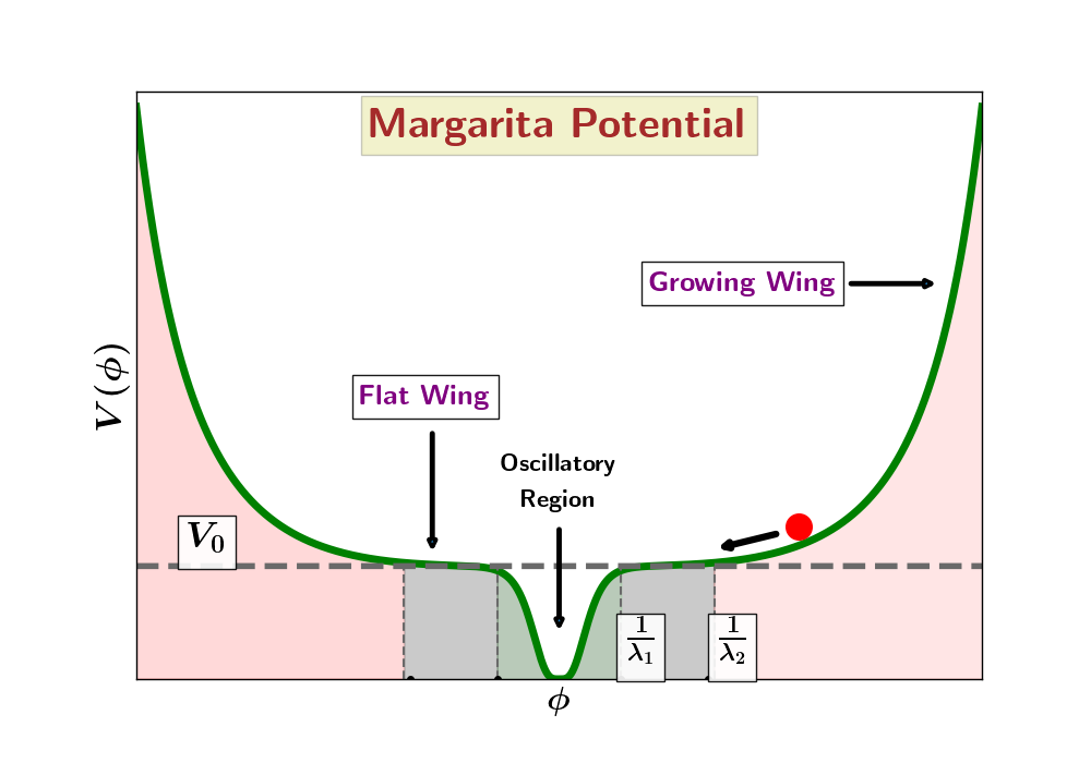
Figure 6: This figure schematically illustrates a typical Margarita potential (4.5) with $\lambda_{1}\gg\lambda_{2}$. For $\lambda_{2}|\phi|\gg m_{p}$, the potential exhibits monotonically growing convex inflationary wings (red shade). For small field values, namely $\lambda_{1}|\phi|\ll m_{p}$, the potential has a minimum (green shade). While for intermediate field values $\frac{1}{\lambda_{1}}<\frac{\phi}{m_{p}}<\frac{1}{\lambda_{2}}$, the potential displays plateau-like behaviour (grey shade).

As a result, a generic Margarita potential will exhibit the following three asymptotic branches (see figure 6) –

$$\mbox{Growing wing:}\quad V(\phi) \simeq {\rm Monotonic}~{},\quad\frac{|\phi|}{m_{p}}\gg\frac{1}{\lambda_{2}}\,,$$ (4.2)

$$\mbox{Flat wing:}\quad V(\phi) \simeq V_{0}+\frac{1}{2}m_{2}^{2}\phi^{2}\,,\quad\frac{1}{\lambda_{1}}\ll\frac{|\phi|}{m_{p}}\ll\frac{1}{\lambda_{2}}\,,$$ (4.3)

$$\mbox{Oscillatory region:}\quad V(\phi) \simeq \frac{1}{2}m_{1}^{2}\phi^{2}\,,\quad\frac{|\phi|}{m_{p}}\ll\frac{1}{\lambda_{1}}\,,$$ (4.4)

where the mass parameters $m_{1}$ and $m_{2}$ depend on $\lambda_{1}$ and $\lambda_{2}$ respectively. Figure 6 illustrates the three asymptotic branches of the Margarita potential.

We first demonstrate the behaviour of Margarita potential by assuming $V_{b}$ to be the T-model based plateau potential [38, 39].

4.1 T-model based exponential Margarita Potential

The Margarita potential in this case is given by

$$V(\phi)=V_{0}\tanh^{2}{\left(\frac{\lambda_{1}\phi}{m_{p}}\right)}\cosh{\left(\frac{\lambda_{2}\phi}{m_{p}}\right)}~{}.$$ (4.5)

where the base potential

$$V_{b}(\phi)=V_{0}\tanh^{2}{\left(\frac{\lambda_{1}\phi}{m_{p}}\right)}~{},$$ (4.6)

is the familiar T-model $\alpha$-attractor potential whose $r$ vs $n_{{}_{S}}$ plot is shown by the red colour curve in figure 4. The correction potential, $V_{c}(\phi)=\cosh{\left(\frac{\lambda_{2}\phi}{m_{p}}\right)}$, has exponential asymptotes for large field values $\lambda_{2}\phi\gg m_{p}$.

In this Margarita potential (4.5), the exponential correction arising from $V_{c}(\phi)=\cosh{\left(\frac{\lambda_{2}\phi}{m_{p}}\right)}$ to the base plateau potential modifies the nature of the $r$ vs $n_{{}_{S}}$ plot, shifting this curve towards higher values of $n_{{}_{S}}$ for identical values of $r$. Hence the $\{n_{{}_{S}},r\}$ predictions of the Margarita potential are, in principle, distinguishable from those of the base T-model potential. This shift is dependent upon the value of the correction parameter $\lambda_{2}$. For $\lambda_{2}=0$, one arrives at the base T-model potential while larger values of $\lambda_{2}$, give rise to a larger shift in the value of $n_{{}_{S}}$ with respect to the base potential. Note that we assume $\lambda_{2}<\sqrt{2}$ in order to realise inflation in the exponential asymptote to $V(\phi)$ at early times. The Margarita potential (4.5) satisfies the CMB constraints on $n_{{}_{S}}$ for $\lambda_{2}\leq 0.1$. Figure 7 shows the $r$ vs $n_{{}_{S}}$ plot of this Margarita potential for $\lambda_{2}=0.04$.

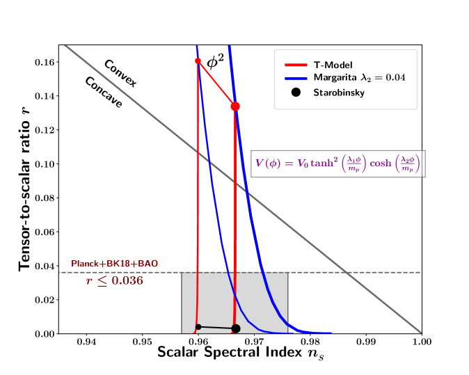
Figure 7: This figure compares the $r$ vs $n_{{}_{S}}$ plot of the Margarita potential (4.5) with its asymptotically flat T-model base potential (4.6) for $\lambda_{2}=0.04$. As usual, the thinner and thicker curves correspond to $N_{*}=50,60$ respectively.

4.2 Implications for initial conditions

As discussed in section 3.2, although recent CMB observations appear to favour asymptotically flat plateau potentials, the latter could face some theoretical shortcomings relating to the issue of initial conditions. In particular, owing to the fact that the height of the plateau saturates to a small value $V_{0}\leq 10^{-10}~{}m_{p}^{4}$ for large field values $\phi\gg m_{p}$, an equipartition of the initial inflaton kinetic energy density $\rho_{\rm KE}=\frac{1}{2}\dot{\phi}^{2}$, potential energy density $\rho_{\rm V}\simeq V_{0}$, and gradient term $\rho_{\rm grd}\simeq\frac{1}{2}(\nabla\phi)^{2}$ will not be possible. Moreover, the possible presence of a large initial curvature density $\rho_{K}=-3\,m_{p}^{2}/a_{i}^{2}$ (corresponding to positive spatial curvature, $K=+1$) might also be problematic for inflation.

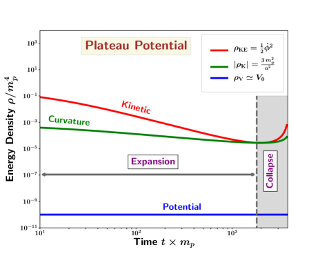
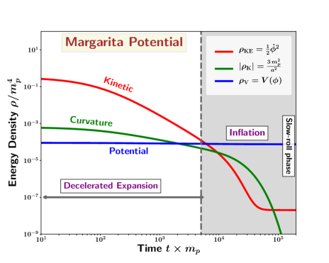
Figure 8: This figure illustrates the implications of a relatively large initial curvature density $\rho_{K}=-3\,m_{p}^{2}/a_{i}^{2}$ (corresponding to a positive spatial curvature, $K=+1$) at the commencement of inflation. The left panel shows the density evolution of the inflaton kinetic term $\rho_{\rm KE}$ (red), potential term $\rho_{V}$ (blue) and the modulus of the spatial curvature term $|\rho_{K}|$ (green) for a plateau potential with $V(\phi)\simeq V_{0}=10^{-10}\,m_{p}^{4}$. The right panel shows the same for the Margarita potential (4.5). From the left panel, we notice that for a plateau potential, even if $\rho_{\rm KE}\gg|\rho_{K}|$ initially, an expanding universe collapses even before inflating due to the small value of $\rho_{V}$ in plateau potentials. By contrast the right panel shows that even though the initial value of $\rho_{V}$ is smaller than the curvature term, the universe keeps expanding and eventually begins to inflate. If one commences from an initial equipartition configuration in which all the three densities are comparable, then realising inflation in a Margarita potential is extremely easy.

To emphasise this point, let us imagine that we set initial conditions for inflation closer to the Planck scale, i.e $\rho_{\phi_{i}}\simeq\,0.1\,m_{p}^{4}$. Suppose the height of the plateau is $V_{0}\simeq 10^{-10}~{}m_{p}^{4}$. In this case, starting from an initial state where the kinetic and curvature densities are of similar magnitude, namely $\rho_{\rm KE}\simeq\rho_{K}\simeq\rho_{\phi_{i}}$, we notice that the universe begins to collapse before inflation begins. This has been demonstrated in the left panel of figure 8 which shows that even an initial curvature density as small as $1\%$ of the initial inflaton energy density leads to the eventual collapse of an initially expanding universe. In fact the initial curvature density must be extremely sub-dominant compared to the initial inflaton energy density in order to prevent the collapse. A preliminary numerical analysis in a forthcoming paper [46] shows that $\rho_{K}<10^{-6}~{}\rho_{\phi_{i}}$ in order for inflation to begin. Hence, unless the spatial curvature is negative or, it is positive with a negligibly small density, plateau potentials are prone to the fine tuning of initial conditions.

However both the equipartition problem and the positive spatial curvature issue can be successfully addressed by a Margarita potential with monotonically growing inflationary wings. This has been demonstrated in the right panel of figure 8. We notice that, starting close to the Planck scale with a relatively large initial curvature density, the universe proceeds to inflate successfully and the collapse scenario can be completely avoided. It is easy to see that the equipartition condition can be easily satisfied in this case. Hence Margarita potentials could play a crucial role in addressing the initial (positive) curvature problem, as well as facilitating the equipartition of initial energy densities of different components, which were amongst the primary goals of inflation in its original formulation [6, 7].

4.3 General recipe for constructing a Margarita potential

The Margarita ‘cocktail glass’ shape of the potential in figure 6 is quite general and not restricted to the potential (4.5) discussed previously.

Indeed a Margarita potential $V(\phi)$ can easily be constructed using the prescription discussed earlier, namely:

• Multiply a plateau-like base potential $V_{b}(\phi)$ with a convex inflationary potential $V_{c}(\phi)$ to make the Margarita potential $V(\phi)$:

  $$V(\phi)=V_{b}(\phi)\times V_{c}(\phi)$$ (4.7)

• Here $V_{b}(\phi)$ must have the following properties:

  1. It vanishes at the origin $V_{b}(\phi=0)=0$.

  2. Its asymptotically flat: $V_{b}(\phi\to\pm\infty)=V_{0}$.

  Examples of some widely studied plateau potentials are:

  1. The KKLT potential [42, 22]

  $$V_{b}(\phi)=V_{0}\frac{\phi^{n}}{\phi^{n}+M^{n}}~{}.$$ (4.8)

  2. The T-model $\alpha$-attractor [42, 22]

  $$V_{b}(\phi)=V_{0}\tanh^{2n}\left(\frac{\alpha\phi}{m_{p}}\right)~{}.$$ (4.9)

  3. The (non-minimally coupled) standard model Higgs potential in the Einstein frame

  $$V(\phi)\simeq V_{0}\,\left(1-e^{-\frac{2}{\sqrt{6}}\frac{|\phi|}{m_{p}}}\right)^{2}~{}.$$ (4.10)

• The convex inflationary potential function $V_{c}(\phi)$ should be dimensionless and preferably symmetric about the origin so that $V_{c}(\phi)=V_{c}(-\phi)$ and $V_{c}(\phi)=1$.

Plateau potential Convex potential Margarita potential $V_{b}(\phi)$ $~{}V_{c}(\phi)$ $~{}V(\phi)=V_{b}(\phi)\times V_{c}(\phi)$ $V_{0}\,\tanh^{2n}\left({\alpha\phi}\right)$ $\cosh{\left({\beta\phi}\right)}$ $V_{0}\,\tanh^{2n}\left({\alpha\phi}\right)\cosh{\left({\beta\phi}\right)}$ $V_{0}\,\frac{\phi^{n}}{\phi^{n}+M^{n}}$ $1+\alpha\phi^{2}$ $V_{0}\,\frac{\phi^{n}}{\phi^{n}+M^{n}}\,(1+\alpha\phi^{2})$ $V_{0}\,\left(1-e^{-\alpha\frac{|\phi|}{m_{p}}}\right)^{2}$ $e^{\beta\phi^{2}}$ $V_{0}\,\left(1-e^{-\alpha\frac{|\phi|}{m_{p}}}\right)^{2}e^{\beta\phi^{2}}$

Table 1: This table lists three base potentials $V_{b}(\phi)$ which are asymptotically flat and three convex potentials $V_{c}(\phi)$. Note that any of the base potentials $V_{b}$ in this table can be multiplied by any of the convex potentials $V_{c}$ to construct the Margarita potential $V(\phi)=V_{b}(\phi)\times V_{c}(\phi)$. ($m_{p}=1$ is assumed in this table).

A list of some plateau base potentials $V_{b}$ and convex potentials $V_{c}$ is given in table 1. Note that any of the base potentials $V_{b}$ in table 1 can be multiplied by any of the convex potentials $V_{c}$ to construct the Margarita potential $V(\phi)=V_{b}(\phi)\times V_{c}(\phi)$. These examples are by no means exhaustive. However a general discussion of the Margarita potential both in the context of inflation and dark energy lies beyond the scope of the present paper.

5 Inflation in the non-canonical framework

Non-canonical scalars have the Lagrangian density [47]

$${\cal L}(X,\phi)=X\left(\frac{X}{M^{4}}\right)^{\alpha-1}-\;V(\phi),~{}~{}~{}~{}X=\frac{1}{2}{\dot{\phi}}^{2}\,,$$ (5.1)

where $M$ has dimensions of mass, while $\alpha\geq 1$ is a dimensionless parameter. When $\alpha=1$ the Lagrangian (5.1) reduces to the usual canonical scalar field Lagrangian ${\cal L}(X,\phi)=X-\;V(\phi)$.

The energy density and pressure have the form

$$\rho_{{}_{\phi}} = \left(2\alpha-1\right)X\left(\frac{X}{M^{4}}\right)^{\alpha-1}+\;V(\phi)\,,$$

$$p_{{}_{\phi}} = X\left(\frac{X}{M^{4}}\right)^{\alpha-1}-\;V(\phi)\,,~{}~{}X\equiv\frac{1}{2}{\dot{\phi}}^{2}\,,$$ (5.2)

which reduces to the canonical expression $\rho_{{}_{\phi}}=X+V$,  $p_{{}_{\phi}}=X-V$ when $\alpha=1$.

One should note that the equation of motion

$${\ddot{\phi}}+\frac{3\,H{\dot{\phi}}}{2\alpha-1}+\left(\frac{V^{\prime}(\phi)}{\alpha(2\alpha-1)}\right)\left(\frac{2\,M^{4}}{{\dot{\phi}}^{2}}\right)^{\alpha-1}=\;0$$ (5.3)

is singular at $\dot{\phi}\rightarrow 0$ and needs to be regularized so that the value of $\ddot{\phi}$ remains finite in this limit. This can be done [24] by modifying the Lagrangian (5.1) to

$${\cal L}_{{}_{R}}(X,\phi)=\left(\frac{X}{1+\beta}\right)\left(1+\beta\left(\frac{X}{M^{4}}\right)^{\alpha-1}\right)-\;V(\phi)\,,$$ (5.4)

where $\beta$ is a dimensionless parameter. In the limit when $\beta\gg 1$, equation (5.3) can be approximated as

$${\ddot{\phi}}\,+\,\frac{3\,H{\dot{\phi}}}{2\alpha-1}\,+\,\left(\frac{V^{\prime}(\phi)}{\epsilon\,+\,\alpha(2\alpha-1)\left(X/M^{4}\right)^{\alpha-1}}\right)\,=\;0,~{}~{}X=\frac{1}{2}{\dot{\phi}}^{2}\,,$$ (5.5)

where $\epsilon\equiv(1+\beta)^{-1}$ is an infinitesimally small correction factor when $\beta>>1$.

As shown in [24] for potentials behaving like $V(\phi)\propto\phi^{p}$ near the minimum, the average EOS during scalar field oscillations is

$$\langle w_{\phi}\rangle=\frac{p\,-\,2\alpha}{p\,(2\alpha-1)\,+\,2\alpha}\,.$$ (5.6)

For $\alpha=1$ the above expression reduces to the canonical result

$$\langle w_{\phi}\rangle=\frac{p-2}{p+2}\,.$$ (5.7)

The inflationary slow-roll parameter $\epsilon_{nc}$ for non-canonical inflation is given by [24]

$$\epsilon_{nc}=\left(\frac{1}{\alpha}\right)^{\frac{1}{2\alpha-1}}\left(\frac{3M^{4}}{V}\right)^{\frac{\alpha-1}{2\alpha-1}}\left(\epsilon_{c}\right)^{\frac{\alpha}{2\alpha-1}}\,,$$ (5.8)

$\epsilon_{c}$ being the canonical slow-roll parameter (3.32). Note that $\epsilon_{nc}<\epsilon_{c}$ for $3M^{4}\ll V$. This suggests that for a fixed potential $V$, the duration of inflation can be enhanced relative to the canonical case ($\alpha=1$), by a suitable choice of $M$.

In the following, we will discuss the inflationary predictions for $\{n_{{}_{S}},r\}$ in the non-canonical framework, starting with the family of monomial power law potentials $V(\phi)\propto\phi^{p}$, followed by the inverse power law potentials $V(\phi)\propto\phi^{-p}$.

5.1 Monomial power law potentials in the non-canonical framework

Monomial power law potentials in the non-canonical framework are described by the Lagrangian density

$${\cal L}(X,\phi)=X\left(\frac{X}{M^{4}}\right)^{\alpha-1}-\;V_{0}\,\left(\frac{\phi}{m_{p}}\right)^{p}\,.$$ (5.9)

Expressions for the scalar spectral index $n_{{}_{S}}$, and the tensor-to-scalar ratio $r$ are given by [24]

$$n_{{}_{S}}=1-2\,\left(\frac{\gamma+p}{2\,\gamma\,N_{*}+p}\right)\,,$$ (5.10)

$$r=\frac{1}{\sqrt{2\alpha-1}}\left(\frac{16\,p}{2\,\gamma\,N_{*}+p}\right)\,,$$ (5.11)

where the parameter $\gamma$ is defined as

$$\gamma=\frac{2\,\alpha+p(\alpha-1)}{2\,\alpha-1}\,.$$ (5.12)

The tensor spectral tilt for non-canonical potentials satisfies the single field consistency relation [24]

$$r=-\frac{8}{\sqrt{2\alpha-1}}\,n_{{}_{T}}\,,$$ (5.13)

which differs from the canonical consistency relation (3.30) for $\alpha>1$, and hence can be used as a smoking gun test for non-canonical inflation.

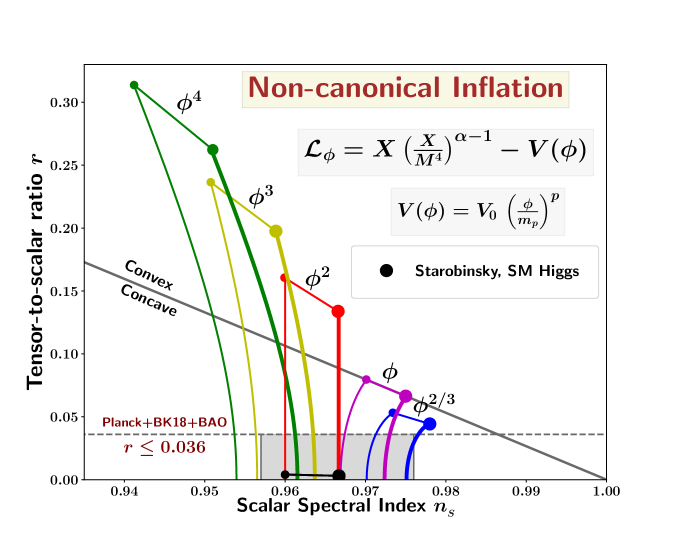
Figure 9: This figure is a plot of the tensor-to-scalar ratio $r$, versus the scalar spectral index $n_{{}_{S}}$, for the monomial power law potentials, $V\propto\phi^{p}$, in the non-canonical framework (5.9) (the thinner and thicker curves correspond to $N_{*}=50,\,60$ respectively). The latest CMB 2$\sigma$ bound $0.957\leq n_{{}_{S}}\leq 0.976$ and the upper bound on the tensor-to-scalar ratio $r\leq 0.036$ are indicated by the shaded grey colour region. The predictions of power law potentials in the non-canonical framework appear to be somewhat similar to those of the T-model potential (3.53) in the canonical framework (see figure 4), with the parameter $\alpha$ in (5.9) playing a role similar to that of $\lambda$ in (3.53). However, for small values of $r$, the $r$ versus $n_{{}_{S}}$ curves of the non-canonical potential , $V\propto\phi^{p}$, do not converge towards a common cosmological attractor for different values of $p$ (in contrast to the attractor behaviour of the T-model, shown in figure 4). Instead, they span virtually the entire parameter space of the observationally allowed region in the $\{n_{{}_{S}},r\}$ plane.

The plots of $r$ versus $n_{{}_{S}}$ in the non-canonical framework for power law potentials $V\propto\phi^{p}$ are shown in figure 9 for different values of $p$. For $\alpha=1$, the predictions of non-canonical power law potentials match with that of the canonical power law potentials, as expected. An increase in the value of $\alpha$ leads to a decrease in the tensor-to-scalar ratio $r$ for all values of $p$. Hence in the non-canonical framework, power law potentials can be consistent with the CMB constraints for large enough values of $\alpha$. In the large $\alpha$ limit, the $\{n_{{}_{S}},r\}$ predictions asymptote to

$$n_{{}_{S}}=1-\frac{3\,p+2}{(p+2)\,N_{*}+p}\,,~{}~{}r=\frac{1}{\sqrt{2\alpha-1}}\left(\frac{16\,p}{(p+2)\,N_{*}+p}\right)\,,~{}{\rm for}~{}\alpha\gg 1\,,$$ (5.14)

which is illustrated in figure 10.

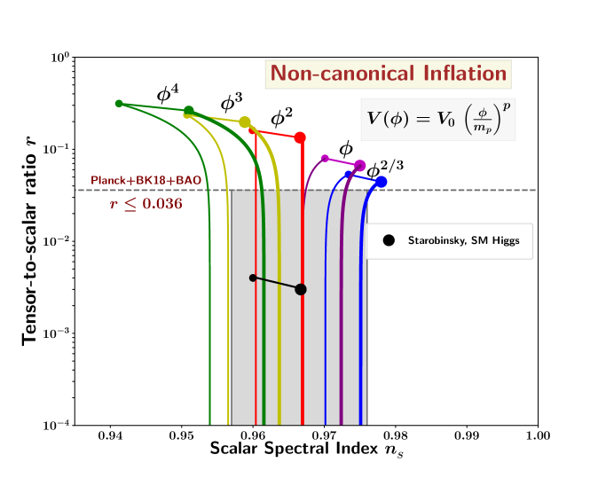
Figure 10: This figure plots the tensor-to-scalar ratio $r$, versus the scalar spectral index $n_{{}_{S}}$, for monomial power law potentials, $V\propto\phi^{p}$, in the non-canonical framework (5.9). The latest CMB 2$\sigma$ bound $0.957\leq n_{{}_{S}}\leq 0.976$ and the upper bound on the tensor-to-scalar ratio $r\leq 0.036$ are indicated by the shaded grey colour region. The tensor-to-scalar ratio $r$ in this figure has been plotted in the logarithmic scale in order to illustrate the asymptotic behaviour of $\{n_{{}_{S}},r\}$ in the limit $\alpha\gg 1$, as given in (5.14), which results in $r\ll 1$. We notice that the $\{n_{{}_{S}},r\}$ predictions in the large $\alpha$ limit are different for different values of $p$, demonstrating the absence of cosmological attractor behaviour which is present in the T-model (3.53) as shown in figure 4.

From figure 9, we notice that the predictions of power law potentials in the non-canonical framework appear to be somewhat similar to that of the T-model potential (3.53) in the canonical framework (see figure 4), with the non-canonical parameter $\alpha$ in (5.9) playing a role similar to that of $\lambda$ in the T-model (3.53). However the $r$ versus $n_{{}_{S}}$ plots in figure 9 are curved lines, in contrast to those in the case of T-model in figure 4 (where they are nearly straight lines). Another important difference is that the predictions of non-canonical power law potentials for different values of $p$, as given in (5.14), do not converge towards a cosmological attractor in the large $\alpha$ limit, in contrast to the predictions of the T-model which approach the cosmological attractor (3.54) independently of the value of $p$. The absence of cosmological attractor behaviour for non-canonical power law potentials implies that they are capable of scanning through the entire parameter space of the observationally allowed region in the $\{n_{{}_{S}},r\}$ plane, as can be seen from figures 9 and 10. Hence they are very important target candidates for future CMB missions.

Before proceeding to discuss inverse power law potentials in the non-canonical framework, we would like to briefly discuss the Standard Model Higgs inflation.

5.2 Standard Model Higgs inflation in the non-canonical framework

The Standard Model (SM) Higgs potential is given by

$$V(\phi)=\frac{\lambda}{4}\left(\phi^{2}-\sigma^{2}\right)^{2}\,,$$ (5.15)

where $\sigma$ is the vacuum expectation value of the SM Higgs field

$$\sigma=246\,{\rm GeV}=1.1\times 10^{-16}\,m_{p}\,,$$ (5.16)

and the Higgs self-coupling constant has the value $\lambda\simeq 0.1$. It would be very interesting if inflation could be sourced by the SM Higgs field. Unfortunately, in the canonical framework, the self-interaction coupling of the Higgs field, $\lambda$ in (5.15), is far too large to be consistent with the small amplitude of scalar fluctuations observed by the CMB which suggest the much smaller value $\lambda\sim 10^{-13}$ [19]. However, this situation can be remedied if either of the following two possibilties is realized:

1. The Higgs couples non-minimally to gravity [27, 28, 26].

2. The Higgs field is described by a non-canonical Lagrangian [24, 26].

In section 3.2, we briefly discussed the first possibility and the corresponding predictions of $\{n_{{}_{S}},r\}$. Here we focus on SM Higgs inflation in the non-canonical framework.

Given that $\sigma=246\,{\rm GeV}\ll m_{p}$, the Higgs potential (5.15) in the limit $\phi\gg\sigma$ takes the form

$$V(\phi)\simeq\frac{\lambda}{4}\phi^{4}\,,$$ (5.17)

which is the quartic monomial power law potential. In the non-canonical framework, the $\{n_{{}_{S}},r\}$ predictions of SM Higgs potential becomes

$$n_{{}_{S}}=1-\left(\frac{\gamma+4}{N_{*}\gamma+2}\right)\,,$$ (5.18)

$$r=\left(\frac{1}{\sqrt{2\,\alpha-1}}\right)\left(\frac{32}{N_{*}\gamma+2}\right)\,,$$ (5.19)

where

$$\gamma\equiv\frac{2(3\alpha-2)}{2\alpha-1}\,.$$ (5.20)

Since $\gamma$ increases from $\gamma=2$ for $\alpha=1$ to $\gamma=3$ for $\alpha\gg 1$, therefore the scalar spectral index increases from the canonical value $n_{{}_{S}}=0.951$ ($\alpha=1,N_{*}=60$) to $n_{{}_{S}}=0.962$, in non-canonical models (with $\alpha\gg 1$). Similarly the tensor-to-scalar ratio $r$ declines with the increase in $\alpha$ as observed before in figure 9. Note that the black colour dots in figure 9 represent the $\{n_{{}_{S}},r\}$ predictions of the non-minimally coupled SM Higgs inflation, while the green curves represent the same for SM Higgs inflation in the non-canonical framework.

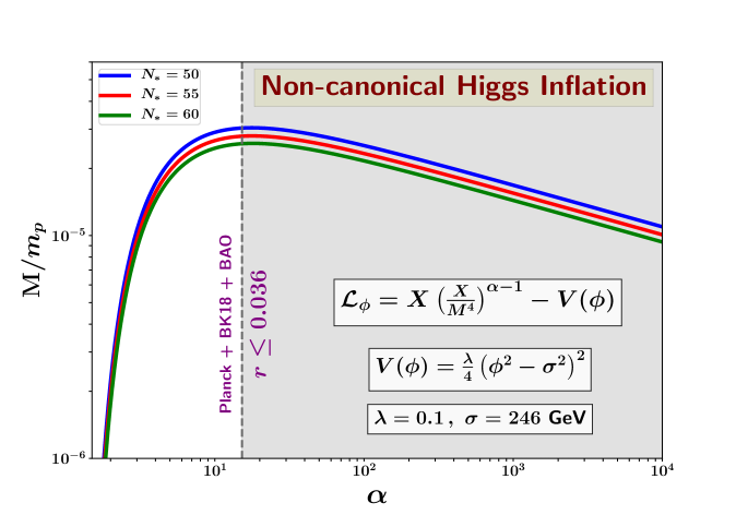
Figure 11: This figure illustrates the relation between the non-canonical parameters $M$ and $\alpha$, given by equation (5.21), for SM Higgs inflation which results in the self-coupling value $\lambda=0.1$ in equation (5.15). Results for three different e-folding values $N_{*}=50,~{}55,~{}60$ are shown by blue, red, and green colour curves respectively. The shaded region corresponds to observationally allowed values of $\alpha$ obeying the CMB constraint $r\leq 0.036$.

The relation between the value of the Higgs self-coupling $\lambda\simeq 0.1$ in the non-canonical framework and the corresponding canonical value $\lambda_{c}$ is given by [26]

$$\lambda=4\left[\frac{32\lambda_{c}(N_{*}+1)^{3}}{\sqrt{2\alpha-1}}\left(\frac{\alpha}{4}\Big{(}\frac{1}{6}\frac{m_{p}^{4}}{M^{4}}\Big{)}^{\alpha-1}\right)^{\frac{2}{3\alpha-2}}\left(\frac{1}{N_{*}\gamma+2}\right)^{\frac{\gamma+4}{\gamma}}\right]^{\frac{3\alpha-2}{\alpha}}\,,$$ (5.21)

where consistency with CMB observations suggests $\lambda_{c}\sim 10^{-13}$.

Figure 11 describes the values of the non-canonical parameters $\alpha$ and $M$ that yield $\lambda\simeq 0.1$ in (5.17) – the relation between $M$ and $\alpha$ being provided by equation (5.21). From our analysis, it is clear that SM Higgs field in the non-canonical framework can successfully source inflation, while obeying the CMB constraints, for large enough values of the non-canonical parameter $\alpha$, as shown by the shaded region in figure 11.

5.3 Inverse power law potentials in the non-canonical framework

It is well known that within the canonical framework a spatially flat universe can expand as a power law with $a(t)\sim t^{q}$, if inflation is sourced by an exponential potential [48]. However, owing to the fact that the tensor-to-scalar ratio $r$ in such models turns out to be much larger than the upper bound set by the CMB observations, namely $r\leq 0.036$, the hope of realising power law inflation is dashed in the canonical framework. Instead, CMB constraints indicate that cosmic expansion is near-exponential if inflation is driven by a canonical scalar field, as discussed in section 3.1.

Nevertheless, power law expansion of the form $a(t)\sim t^{q}$ with $q>1$, can also be realised in the non-canonical framework (5.1) with an inverse power law(IPL) potential [25]

$$V(\phi)=V_{0}\left(\frac{\phi}{m_{p}}\right)^{-p}\,,$$ (5.22)

where $p$ is related to the non-canonical parameter $\alpha$ by [25]

$$p=\frac{2\,\alpha}{\alpha-1}\,,$$ (5.23)

and the expansion rate, $a(t)\sim t^{q}$, is related to the EOS of the scalar field by the usual relation

$$q=\frac{2}{3}\,\left(\frac{1}{1+w_{\phi}}\right)\,.$$ (5.24)

Expressions for the scalar spectral index $n_{{}_{S}}$, and the tensor-to-scalar ratio $r$ in the non-canonical framework are given by [25]

$$n_{{}_{S}}=1-\frac{2}{q-1}\,,$$ (5.25)

$$r\simeq\frac{16}{q\,\sqrt{2\,\alpha-1}}\,,$$ (5.26)

where the ‘$\simeq$’ symbol in the expression of $r$ refers to the fact that the above equation is valid in the slow-roll limit $q\gg 1$. From expressions (5.25) and (5.26), we notice that the scalar spectral tilt $n_{{}_{S}}$ does not depend upon the non-canonical parameter $\alpha$, while the tensor-to-scalar ratio $r$ decreases with an increase in $\alpha$. Hence for large enough values of $\alpha$, the IPL potential can satisfy the CMB constraints in the non-canonical framework, as shown in figure 12.

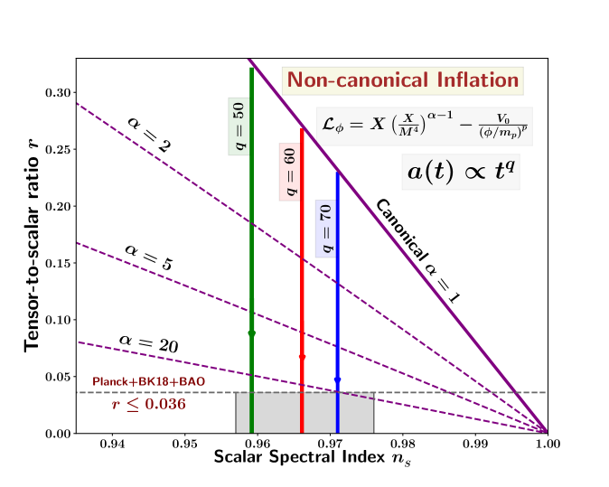
Figure 12: This figure is a plot of the tensor-to-scalar ratio $r$, versus the scalar spectral index $n_{{}_{S}}$, for the inverse power law (IPL) potential (5.22) in the non-canonical framework, which leads to power law inflation $a(t)\sim t^{q}$, $q\gg 1$. The latest CMB 2$\sigma$ bound $0.957\leq n_{{}_{S}}\leq 0.976$ and the upper bound on the tensor-to-scalar ratio $r\leq 0.036$ are indicated by the shaded grey colour region. The green, red, and blue colour curves correspond to $q=50\,,60\,,70$ respectively. For a given value of $q$, while $n_{{}_{S}}$ is insensitive to the value of the non-canonical parameter $\alpha$, the tensor-to-scalar ratio $r$ decreases with an increase in $\alpha$, which has been illustrated by the arrow marks on each plot. The purple lines represent contours of fixed $\alpha$ values. For $\alpha>20$ and $q\in[47.5,\,84.3]$, predictions of the non-canonical IPL potential are consistent with CMB constraints.

From expression (5.25), the CMB constraints (3.40) on the scalar spectral index $n_{{}_{S}}$ translate into $q\in[47.5,\,84.3]$. Figure 12 depicts the behaviour of $r$ versus $n_{{}_{S}}$ for three different values of expansion exponent, namely $q=50\,,60\,,70$, plotted in green, red, and blue colour curves respectively. The arrow mark on each plot indicates the direction of increase in the value of $\alpha$. From this figure, it is easy to see that the CMB constraints, shown by the grey colour shaded region, can easily be satisfied for $\alpha>20$. Hence power law inflation can be successfully sourced by the IPL potential in the non-canonical framework, without violating the CMB bounds on $\{n_{{}_{S}},r\}$.

Graceful exit from power law inflation

During power law inflation, since the universe accelerates forever, it does not account for the end of inflation and the subsequent transition into the radiative hot Big Bang phase. This issue of ‘graceful exit’ from the inflationary phase turns out to be one of the central drawbacks of power law inflation. A possible way out is to assume that the potential driving power law inflation approximates a more general functional form which allows for the oscillations of the inflaton field at the end of inflation and hence results in a successful reheating scenario. An interesting general form of the potential in the context of non-canonical inflation is [25]

$$V(\phi)=V_{0}\left[\left(\frac{\phi}{m_{p}}\right)^{p/2}-\left(\frac{\phi}{m_{p}}\right)^{-p/2}\right]^{2}\,,$$ (5.27)

with $p=2\alpha/(\alpha-1)$ as given in (5.23). The potential is schematically shown in figure 13.

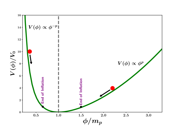
Figure 13: This figure schematically depicts the inflationary potential (5.27) which can address the graceful exit problem of power law inflation in the non-canonical framework. For $\phi<m_{p}$, the potential exhibits inverse power law behaviour $V(\phi)\sim\phi^{-p}$ which results in power law inflation in the non-canonical framework. For $\phi>m_{p}$, the potential exhibits monomial behaviour $V(\phi)\sim\phi^{p}$ which results in quasi-exponential inflation. After the end of inflation, the non-canonical scalar field oscillates around the minimum of the potential at $\phi=m_{p}$, resulting in successful reheating of the universe.

For $\phi<m_{p}$, the potential has the asymptotic form $V(\phi)\sim\phi^{-p}$ which leads to power law inflation in the non-canonical framework. While for $\phi>m_{p}$, the potential exhibits monomial behaviour $V(\phi)\sim\phi^{p}$ which leads to quasi-exponential inflation. After the end of inflation, the non-canonical scalar field oscillates around the minimum of the potential which is located at $\phi=m_{p}$, resulting in successful reheating.

6 Discussion

The latest CMB results from the BICEP/Keck collaboration [21], combined with the PLANCK 2018 data release [19], have imposed a stringent upper bound on the primordial tensor-to-scalar ratio $r\leq 0.036$ (at $95\%$ confidence). Additionally, CMB observations constrain the scalar spectral tilt to be $n_{{}_{S}}\in[0.957,0.976]$ at the 2$\sigma$ level. In this paper, we have discussed the implications of these latest CMB constraints on inflationary models, with particular emphasis on inflation sourced by a scalar field with a non-canonical Lagrangian density.

In section 3, we discussed the implications of the latest CMB constraints on the primordial observables $\{n_{{}_{S}},r\}$ in the framework of slow-roll inflation driven by a single canonical scalar field $\phi$ with a potential $V(\phi)$. The upper bound on the tensor-to-scalar ratio $r\leq 0.036$ strongly disfavours monotonically increasing convex inflationary potentials within the canonical framework. In fact, one of the central inferences that can be drawn from the CMB constraints is the fact that the entire family of monomial power law potentials $V(\phi)\sim\phi^{p}$ are now completely ruled out in the canonical framework. Among these, are the simplest classic inflationary models including the $\frac{1}{2}m^{2}\phi^{2}$ and $\lambda\phi^{4}$ potentials. Instead, the CMB data now favours asymptotically flat plateau like potentials. In section 3.2, we discussed a number of important plateau potentials in light of the latest observational constraints, including the Einstein frame potentials associated with Starobinsky inflation and non-minimally coupled Higgs inflation, as well as the T-model and E-model $\alpha$-attractors and the D-brane KKLT inflation. The $\{n_{{}_{S}},r\}$ predictions of these models are illustrated in figure 2. In the limit $r\ll 1$, the $\{n_{{}_{S}},r\}$ predictions of $\alpha$-attractor potentials exhibit an attractor behaviour [42, 22] as illustrated in figure 4 for the T-model. We demonstrated that plateau potentials generically produce a small tensor-to-scalar ratio and hence are consistent with the CMB data, in agreement with earlier results [42, 22].

However, for large field values, the plateau potentials saturate to a constant value $V_{0}$ which is typically small, namely $V_{0}\leq 10^{-10}\,m_{p}^{4}$ for $r\ll 1$. The small height of a plateau potential bears significant implications for the issue of initial conditions for inflation. Owing to the fact that the plateau height is typically very small compared to the Planck scale, an equipartition of the initial kinetic, potential, and gradient energy terms is not possible at very early times when initial conditions for inflation are usually set. Similarly, the initial presence of positive spatial curvature could also be problematic for inflation with plateau potentials. Additionally, for $r\ll 1$, plateau potentials might exhibit a large running of the scalar spectral tilt $n_{{}_{S}}$ as recently pointed out in [44]. Due to the aforementioned reasons, we focus on scenarios where monotonically increasing convex potentials can be accommodated by the CMB data. In this connection, we study two types of models. The first one is the Margarita potential formulated in the canonical framework, while the second scenario is associated with non-canonical Lagrangians of the form ${\cal L}=X^{\alpha}-V(\phi)$,   $\alpha\geq 1$ ($X={\dot{\phi}}^{2}/2$).

In section 4, we introduced the Margarita potential (4.1) which features a monotonically growing convex inflationary wing at the commencement of a plateau potential. We discussed the $\{n_{{}_{S}},r\}$ predictions of a specific Margarita potential (4.5) constructed by incorporating extensions to the T-model potential at large field values. We demonstrated that Margarita potentials easily satisfy CMB constraints and also allow for an equipartition between initial energy densities. We also discussed a general recipe for constructing Margarita potentials.

Section 5 was dedicated to the study of inflation in the non-canonical framework [24, 25] in the light of the recent CMB data release. In section 5.1, working with the family of power law potentials $V(\phi)\sim\phi^{p}$, we demonstrated that inflation with monomial power law potentials can be successfully resurrected in the non-canonical framework. In particular, we compared and contrasted the $\{n_{{}_{S}},r\}$ predictions of non-canonical power law potentials shown in figure 9 against those of the T-model $\alpha$-attractor potential in the canonical framework shown in figure 4. We found that CMB predictions of power law potentials in non-canonical inflation do not exhibit attractor behaviour, which stands in contrast to the predictions of $\alpha$-attractors. Instead, they span the entire parameter space of the observationally allowed region in the $\{n_{{}_{S}},r\}$ plane. This is one of the central results of our analysis. In section 5.2, we discussed the possibility of realising successful inflation with the Standard Model Higgs potential in the non-canonical framework. We showed that the non-canonical Higgs with standard model parameters could easily satisfy CMB constraints.

Section 5.3 was devoted to a study of inflation with inverse power law (IPL) potentials $V(\phi)\sim\phi^{-p}$ in the non-canonical framework. IPL potentials within the non-canonical framework lead to power law inflation with $a(t)\sim t^{q}$ [25]. We demonstrated that the $\{n_{{}_{S}},r\}$ predictions of IPL potentials are consistent with the CMB data for sufficiently large values of the non-canonical parameter $\alpha>20$, as shown in figure 12. We also discussed a remedy to the graceful exit problem for power law inflation in the non-canonical framework.

Finally we would like to draw attention to the fact that the analysis of initial conditions for inflation with plateau potentials [26] remains an interesting open area of research, especially in presence of a positive spatial curvature [49, 50]. We shall study this in more detail in a companion work [46]. However, we would also like to emphasise that regardless of the issue of initial conditions, both power law and inverse power law potentials in the non-canonical framework (and the Margarita potential in the canonical framework), satisfy current CMB constraints and are therefore important target candidates for the next generation of CMB missions.

7 Acknowledgements

S.S.M. is supported as a postdoctoral Research Associate at the Centre for Astronomy and Particle Theory, University of Nottingham by the STFC funded consolidated grant, UK. Varun Sahni was partially supported by the J. C. Bose Fellowship of Department of Science and Technology, Government of India.

References

- [1] N. Aghanim et al. [Planck], “Planck 2018 results. VI. Cosmological parameters,” Astron. Astrophys. 641, A6 (2020) [arXiv:1807.06209 [astro-ph.CO]].
- [2] V. A. Rubakov and D. S. Gorbunov, “Introduction to the Theory of the Early Universe: Hot big bang theory, World Scientific, Singapore, 2011, doi:10.1142/10447.
- [3] V. A. Rubakov and D. S.Gorbunov, “Introduction to the Theory of the Early Universe: Cosmological perturbations and inflationary theory, World Scientific, Singapore, 2011, doi:10.1142/7874.
- [4] L. Perivolaropoulos and F. Skara, “Challenges for CDM: An update,” [arXiv:2105.05208 [astro-ph.CO]].
- [5] A. A. Starobinsky, “A New Type of Isotropic Cosmological Models Without Singularity,” Phys. Lett. B 91, 99-102 (1980).
- [6] A. H. Guth, “The Inflationary Universe: A Possible Solution to the Horizon and Flatness Problems,” Phys. Rev. D 23, 347 (1981).
- [7] A. D. Linde, “A New Inflationary Universe Scenario: A Possible Solution of the Horizon, Flatness, Homogeneity, Isotropy and Primordial Monopole Problems”, Phys. Lett. B 108, 389 (1982).
- [8] A. Albrecht and P. J. Steinhardt, “Cosmology for Grand Unified Theories with Radiatively Induced Symmetry Breaking,” Phys. Rev. Lett. 48, 1220 (1982).
- [9] A. D. Linde, “Chaotic Inflation,” Phys. Lett. B 129, 177-181 (1983).
- [10] A.D. Linde, Particle Physics and Inflationary Cosmology, Harwood, Chur, Switzerland (1990).
- [11] D. Baumann, “TASI Lectures on Inflation”, [arXiv:0907.5424].
- [12] V. F. Mukhanov and G. V. Chibisov, JETP Lett. 33, 532 (1981).
- [13] S. W. Hawking, Phys. Lett. B 115, 295 (1982).
- [14] A. A. Starobinsky, Phys. Lett. B 117, 175 (1982).
- [15] A. H. Guth and S. -Y. Pi, Phys. Rev. Lett. 49, 1110 (1982).
- [16] A.A. Starobinsky, JETP Lett., 30 , 682 (1979).
- [17] V. Sahni, Phys. Rev. D42, 453 (1990).
- [18] M. Tegmark, “What does inflation really predict?,” JCAP 04 (2005), 001 [arXiv:astro-ph/0410281 [astro-ph]].
- [19] Y. Akrami et al. [Planck], “Planck 2018 results. X. Constraints on inflation” Astron. Astrophys. 641, A10 (2020) [arXiv:1807.06211 [astro-ph.CO]].
- [20] S. S. Mishra, V. Sahni and A. A. Starobinsky, “Curing inflationary degeneracies using reheating predictions and relic gravitational waves,” JCAP 05, 075 (2021) [arXiv:2101.00271 [gr-qc]].
- [21] P. A. R. Ade et al. [BICEP and Keck], “Improved Constraints on Primordial Gravitational Waves using Planck, WMAP, and BICEP/Keck Observations through the 2018 Observing Season,” Phys. Rev. Lett. 127, no.15, 151301 (2021) [arXiv:2110.00483 [astro-ph.CO]].
- [22] R. Kallosh and A. Linde, “BICEP/Keck and cosmological attractors,” JCAP 12, no.12, 008 (2021) [arXiv:2110.10902 [astro-ph.CO]].
- [23] A. Ijjas, P. J. Steinhardt and A. Loeb, “Inflationary paradigm in trouble after Planck2013,” Phys. Lett. B 723, 261-266 (2013) [arXiv:1304.2785 [astro-ph.CO]].
- [24] S. Unnikrishnan, V. Sahni and A. Toporensky, “Refining inflation using non-canonical scalars,” JCAP 08, 018 (2012) [arXiv:1205.0786 [astro-ph.CO]].
- [25] S. Unnikrishnan and V. Sahni, “Resurrecting power law inflation in the light of Planck results,” JCAP 10, 063 (2013) [arXiv:1305.5260 [astro-ph.CO]].
- [26] S. S. Mishra, V. Sahni and A. V. Toporensky, “Initial conditions for Inflation in an FRW Universe,” Phys. Rev. D 98, no.8, 083538 (2018) [arXiv:1801.04948 [gr-qc]].
- [27] R. Fakir and W.G. Williams, Phys. Rev. D 41, 1783-1791 (1990).
- [28] F. L. Bezrukov and M. Shaposhnikov, Phys. Lett. B 659, 703-706 (2008) [arXiv:0710.3755].
- [29] R. Brandenberger, “Initial conditions for inflation — A short review,” Int. J. Mod. Phys. D 26 (2016) no.01, 1740002 [arXiv:1601.01918 [hep-th]].
- [30] A.R. Liddle and D.H. Lyth, Cosmological Inflation and Large Scale Structure, Cambridge University Press, 2000.
- [31] D. Baumann, PoS TASI 2017, 009 (2018) [arXiv:1807.03098 [hep-th]].
- [32] M. Sasaki, “Large Scale Quantum Fluctuations in the Inflationary Universe,” Prog. Theor. Phys. 76, 1036 (1986).
- [33] V. F. Mukhanov, “Quantum Theory of Gauge Invariant Cosmological Perturbations,” Sov. Phys. JETP 67, 1297 (1988) [Zh. Eksp. Teor. Fiz. 94N7, 1 (1988)].
- [34] H. Motohashi, A. A. Starobinsky and J. Yokoyama, “Inflation with a constant rate of roll,” JCAP 1509, 018 (2015) [arXiv:1411.5021 [astro-ph.CO]].
- [35] T. S. Bunch and P. C. W. Davies, “Quantum Field Theory in de Sitter Space: Renormalization by Point Splitting,” Proc. Roy. Soc. Lond. A 360, 117 (1978).
- [36] J. Martin, C. Ringeval and V. Vennin, “Encyclopædia Inflationaris,” Phys. Dark Univ. 5-6 (2014), 75-235 [arXiv:1303.3787 [astro-ph.CO]].
- [37] B. Whitt, “Fourth Order Gravity as General Relativity Plus Matter,” Phys. Lett. B 145, 176-178 (1984).
- [38] R. Kallosh and A. Linde, “Universality Class in Conformal Inflation,” JCAP 07, 002 (2013) [arXiv:1306.5220 [hep-th]].
- [39] R. Kallosh, A. Linde and D. Roest, “Superconformal Inflationary -Attractors,” JHEP 11, 198 (2013) [arXiv:1311.0472 [hep-th]].
- [40] S. Kachru, R. Kallosh, A. D. Linde and S. P. Trivedi, “De Sitter vacua in string theory,” Phys. Rev. D 68, 046005 (2003) [arXiv:hep-th/0301240 [hep-th]].
- [41] S. Kachru, R. Kallosh, A. D. Linde, J. M. Maldacena, L. P. McAllister and S. P. Trivedi, “Towards inflation in string theory,” JCAP 0310, 013 (2003) [hep-th/0308055].
- [42] R. Kallosh and A. Linde, “CMB targets after the latest Planck data release,” Phys. Rev. D 100, no.12, 123523 (2019) [arXiv:1909.04687 [hep-th]].
- [43] F. L. Bezrukov and D. S. Gorbunov, “Distinguishing between R2-inflation and Higgs-inflation,” Phys. Lett. B 713, 365-368 (2012) [arXiv:1111.4397 [hep-ph]].
- [44] R. Easther, B. Bahr-Kalus and D. Parkinson, “Born to Run: Inflationary Dynamics and Observational Constraints,” [arXiv:2112.10922 [astro-ph.CO]].
- [45] S. Bag, S. S. Mishra and V. Sahni, “New tracker models of dark energy,” JCAP 08, 009 (2018) [arXiv:1709.09193 [gr-qc]].
- [46] S. S. Mishra and V. Sahni and A. V. Toporensky “Initial conditions for inflation in an FLRW universe with a positive spatial curvature,” (in preparation).
- [47] V. F. Mukhanov and A. Vikman, “Enhancing the tensor-to-scalar ratio in simple inflation,” JCAP 02, 004 (2006) [arXiv:astro-ph/0512066 [astro-ph]].
- [48] F. Lucchin and S. Matarrese, “Power Law Inflation,” Phys. Rev. D 32, 1316 (1985).
- [49] A. Linde, “Inflationary Cosmology after Planck 2013,” [arXiv:1402.0526 [hep-th]].
- [50] A. H. Guth, D. I. Kaiser and Y. Nomura, “Inflationary paradigm after Planck 2013,” Phys. Lett. B 733, 112-119 (2014) [arXiv:1312.7619 [astro-ph.CO]].