Hyperbolic Lattice for Scalar Field Theory in AdS₃

Abstract

We construct a tessellation of AdS₃, by extending the equilateral triangulation of AdS₂ on the Poincaré disk based on the $(2,3,7)$ triangle group, suitable for studying strongly coupled phenomena and the AdS/CFT correspondence. A Hamiltonian form conducive to the study of dynamics and quantum computation is presented. We show agreement between lattice calculations and analytic results for the free scalar theory and find evidence of a second order critical transition for $\phi^{4}$ theory using Monte Carlo simulations. Applications of this AdS Hamiltonian formulation to real time evolution and quantum computing are discussed.

1 Introduction

The study of strongly coupled Quantum Field Theories (QFTs) is difficult, even before putting them in anti-de Sitter (AdS) space. Yet there are compelling reasons to understand the full non-perturbative consequences Callan:1989em of doing so. The general AdS/CFT duality maps any ultraviolet (UV) renormalizable field theory in bulk AdS_d+1 to a $d$-dimensional Conformal Field Theory (CFT_d) on the boundary. Despite the spectacular results of the conformal bootstrap program in bounding CFTs with a conserved stress tensor (e.g., Rattazzi:2008pe ; El-Showk:2012cjh ), there is still a huge landscape of non-perturbative field theories in AdS yet to be explored with potential applications to particle and condensed matter physics. Moreover, in three dimensions AdS₃ gives the interesting and special case of a two-dimensional boundary CFT₂. It is also the minimum dimensionality needed to study the map between non-trivial pure weak gravity and CFT with a conserved stress tensor.

The best developed numerical framework for solving strongly coupled QFTs at the moment is lattice field theory. This method has benefited from decades of development of efficient algorithms and high performance architectures to produce extremely precise predictions for physical systems such as Quantum Chromodynamics ExascaleWP . To best utilize this framework, lattice QCD and similar problems are posed as a path integral in flat Euclidean space, which benefits from a regular lattice with a uniform UV cut-off and a positive definite measure allowing for the efficient use of parallelized Monte Carlo algorithms.

Adapting lattice field theory to AdS space presents two new problems: (i) lattices must conform to a curved manifold and (ii) the finite lattice volume must have a boundary that maps to a CFT at infinite distances. The first problem (i) has largely been addressed in the Quantum Finite Element (QFE) program by introducing a simplicial lattice complex weighted by the discrete exterior calculus Brower:2016vsl ; Brower:2018szu ; Brower:2020jqj ; brower2021PoS . QFE is proving to give accurate results for the $\phi^{4}$ Ising CFT in 2D on the Riemann sphere ${\mathbb{S}}^{2}$ and in 3D for the radially quantized cylinder ${\mathbb{R}}\times{\mathbb{S}}^{2}$.

The extension of QFE to a hyperbolic manifold was presented in Brower:2019kyh for AdS₂. In addition, for AdS₂ the second problem (ii) of convergence as a function of the UV cut-off to the boundary CFT was shown to be feasible at finite volumes. In this work we extend this investigation by choosing a foliation for global Euclidean AdS_d+1 that defines the Hamiltonian (dilatation) operator dual to the boundary CFT in the radially quantized formulation on ${\mathbb{R}}\times{\mathbb{S}}^{d}$. In 3D this particular AdS₃ geometry allows for the re-use of the basic lattice scaffolding of the Poincaré disk ${\mathbb{H}}^{2}$ by tessellating each 2D slice via the triangle group at fixed time. This lattice field theory approach to the non-perturbative study of QFTs in AdS space is complementary to the S-matrix bootstrap approach Paulos:2016fap ; Paulos:2016but as well as increasingly powerful Hamiltonian truncation methods Rychkov:2015vap ; Hogervorst:2021spa ; Anand:2020qnp . The use of the Hamiltonian formulation of lattice field theory opens up potential applications to Minkowski space complementary to the light-cone truncation method Katz:2016hxp ; Anand:2020gnn and generally to quantum computing algorithms.

This article begins in Sec. 2 with a general discussion of the AdS manifold and our lattice construction of AdS₃. Section 3 details the Hamiltonian and Lagrangian formulation of $\phi^{4}$ theory on the lattice. Section 4 focuses on the free theory, where we compute various propagators directly to compare the lattice to the continuum and as a check of our Monte Carlo methods. Section 5 then uses these methods to demonstrate evidence for the existence of a second order critical point in $\phi^{4}$ theory in AdS₃. We finish in Sec. 6 with a discussion of future directions for high precision Monte Carlo simulations for both $\phi^{4}$ and Ising spins in AdS₃ to probe the AdS/CFT correspondence, as well as using the Hamiltonian form as a prototype for quantum computing algorithms.

2 Anti-de Sitter Space

We begin with a general discussion about AdS space and its various foliations before proceeding to its latticization. Euclidean AdS_d+1 with curvature radius $\ell$ is a space of constant negative curvature defined as the hyperboloid,

$$-X^{2}_{0}+\vec{X}\cdot\vec{X}=-X_{0}X_{0}+\sum_{i=1}^{d+1}X_{i}X_{i}=-\ell^{2}\;,\quad\quad X_{0}>0\;,$$ (2.1)

embedded in $\mathbb{R}^{1,d+1}$ and possessing the isometries of the Euclidean conformal group $SO(1,d+1)$. Between any two points $X$, $X^{\prime}$ on the manifold, there exists a unique geodesic given by

$$\ell^{2}\cosh(\sigma(X,X^{\prime}))=X_{0}X^{\prime}_{0}-\vec{X}\cdot\vec{X}^{\prime}\geq 0\;,$$ (2.2)

which, when projected onto the hyperbolic surface is a positive spacelike distance as seen by the alternative expression $\ell^{2}\sinh^{2}(\sigma/2)=(\vec{X}-\vec{X}^{\prime})^{2}-(X_{0}-X^{\prime}_{0})^{2}$.

Before constructing a lattice it is useful to think about the choice of coordinates taken on the hyperbolic surface Bengtsson98 . Three conventional ones are the Upper Half-Plane (UHP), the Poincaré ball, and the AdS cylinder (see Fig. 1). The boundary CFTs for these three coordinate systems are on different manifolds: Euclidean ${\mathbb{R}}^{d}$, the sphere ${\mathbb{S}}^{d}$, and the cylinder ${\mathbb{R}}\times{\mathbb{S}}^{d-1}$, respectively. For each choice, the hyperbolic manifold remains unchanged while the boundary CFT maps to different manifolds related by Weyl factors. This well known fact is emphasized by Witten Witten:1998qj but is sometimes obscured by referring to both the Weyl equivalences and isometries of AdS space as “conformal”.

Euclidean AdS_d+1 has the topology of a cylinder ${\mathbb{R}}\times{\mathbb{H}}^{d}$ with its metric being the sum of two terms,

$$ds^{2}=g_{00}dt^{2}+ds^{2}_{\mathbb{H}^{d}}\;,$$ (2.3)

which separates Euclidean time $t\in(-\infty,\infty)$ from the spatial metric on $\mathbb{H}^{d}$. Time translation is generated by the dilatation operator $D=-\partial_{t}$ (or AdS Hamiltonian) with unitary evolution in Minkowski space corresponding to the replacement $t\rightarrow-it$. The temporal metric component $g_{00}$ is a function of a radial coordinate on ${\mathbb{H}}^{d}$, but causal propagation in the bulk is consistent with causality in the boundary CFT berenstein:2021 .

A particularly nice foliation for AdS is given by global coordinates,

$$ds^{2}=\pm\ell^{2}\cosh^{2}\rho\,dt^{2}+\ell^{2}(d\rho^{2}+\sinh^{2}\rho\,d\Omega_{d-1}^{2})\;,$$ (2.4)

where $\rho\in[0,\infty]$ is the geodesic from the origin of ${\mathbb{H}}^{d}$ at fixed time with $g_{00}(\rho)=\ell^{2}\cosh(\rho)$ and $d\Omega^{2}_{d-1}$ is the line element of the unit sphere ${\mathbb{S}}^{d-1}$. The minus sign is for Minkowski AdS whereas the plus sign gives Euclidean AdS. For AdS₃ this is then

$$ds^{2}=\ell^{2}(\cosh^{2}\rho\,dt^{2}+d\rho^{2}+\sinh^{2}\rho\,d\theta^{2})\;,$$ (2.5)

with $d\Omega^{2}_{1}=d\theta^{2}$ on ${\mathbb{S}}^{1}$.

In global coordinates the conformal boundary is at $\rho=\infty$. By compactifying the radial coordinate through $r=\tanh(\rho/2)$ we obtain the Poincaré disk coordinates,

$$ds^{2}=\frac{\ell^{2}}{(1-r^{2})^{2}}\left((1+r^{2})^{2}dt^{2}+4(dr^{2}+r^{2}d\theta^{2})\right)\;,$$ (2.6)

which include the conformal boundary at $r=1$. This form of the line element makes particularly clear the cylindrical topology, i.e., the time translation and $SO(2)$ symmetry. In practice, a UV cut-off $\epsilon=1-r_{\text{max}}=\mathcal{O}(e^{-\rho_{\text{max}}})$ is introduced for the boundary CFT at $r=1$. A picture of AdS₃ spacetime is shown in Fig. 1.

We note that for AdS₂ with $d=1$, the cylindrical form of the metric is reduced to an infinite strip via the change of variables $\cosh\rho=1/\cos(\sigma)$. The metric (2.4) is then given by

$$ds^{2}=\ell^{2}(\cosh^{2}\rho\,dt^{2}+d\rho^{2})=\frac{\ell^{2}}{\cos^{2}\sigma}[dt^{2}+d\sigma^{2}]\;,$$ (2.7)

with $\sigma\in[-\pi/2,\pi/2]$ and the 1D conformal quantum mechanics exists on the boundary at $\sigma=\pm\pi/2$. This form is convenient for the Hamiltonian truncation methods presented in Hogervorst:2021spa .

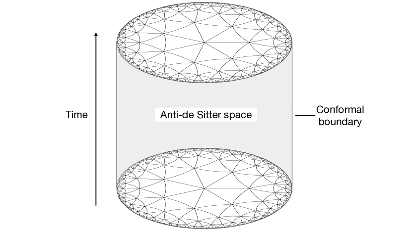
Figure 1: AdS₃ spacetime with our choice of coordinate system looks like a solid cylinder. At fixed time the space is the hyperbolic disk, which can be tessellated using equilateral hyperbolic triangles. Here, $(2,3,7)$ triangles are used.

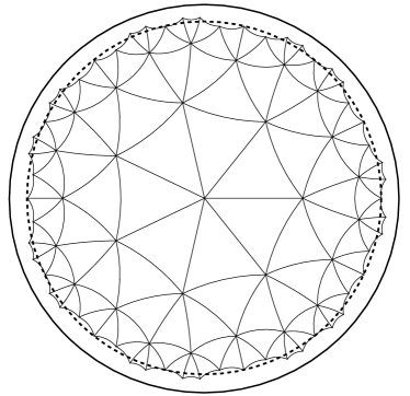
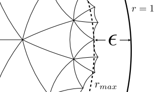
Figure 2: The full hyperbolic disk ${\mathbb{H}}^{2}$ and a zoomed in view of the edge, tessellated with three layers $(L=3)$ of $(2,3,7)$ triangles. The dashed circle near the lattice edge is the effective lattice boundary $r_{\text{max}}$ and the larger, solid circle the conformal boundary at $r=1$. The UV lattice cut-off is $\epsilon=1-r_{\text{max}}$.

2.1 Choosing the spatial lattice

A lattice field theory calculation replaces the continuum manifold with a finite lattice spacing $a$ (UV cut-off) and a finite volume $V$ (IR cut-off). For example, for the $d$-dimensional flat space cubic lattice with toroidal boundary conditions with $V=\mathcal{O}(L_{1}L_{2}\cdots L_{d})$ and $\mathcal{O}(L_{\mu}/a)$ lattice sites on each axis, the lowest mass $m\sim 1/\xi$ (or gap) must obey $a\ll\xi\ll L_{\mu}$ in the numerical extrapolation to the continuum, $a\rightarrow 0,~{}L_{\mu}\rightarrow\infty$. In principle, to obtain the correct boundary CFT these limits precede the conformal limit $\xi\rightarrow\infty$. Since AdS space contains an intrinsic radius of curvature, $\ell$, we can only access the critical point with the proviso that $a\ll\ell\ll\rho_{\text{max}}$.

Given the orthogonality in the metric (2.3), it is natural to foliate Euclidean AdS into fixed time slices transverse to the spatial ${\mathbb{H}}^{d}$ metric and then subsequently introduce a spatial lattice for each time slice. For AdS₃ the spatial tessellation is identical to the lattice realization for $\mathbb{H}^{2}$ detailed in Brower:2019kyh . The hyperbolic disk can then be tessellated using equilateral triangles of the $(2,3,q)$ triangle group for $q>6$. Throughout this work we use $q=7$ because it gives the smallest equilateral hyperbolic triangle edge length (relative to $\ell$), which minimizes the curvature defects at the vertices. A complementary way to latticize AdS₃ using a regular tessellation of ${\mathbb{H}}^{3}$ is done in Asaduzzaman_2020 .

This construction, not unlike the tessellation of the flat plane with equilateral triangles $(q=6)$, gives an infinite lattice with a discrete subgroup of the AdS₂ isometries: invariance under translations along the edges and q-fold rotations about each vertex. On a hyperbolic lattice, these symmetries are then broken by finite volume effects when introducing an IR cut-off $\rho_{x}\leq\rho_{\text{max}}$ with an arbitrary center at $\rho=0$. Using the triangle group, the lattice spacing is now fixed relative to the curvature. For example, for $(2,3,q)$ the deficit angle fixes the equilateral triangle area to $A_{\Delta}=(\pi-6\pi/q)\ell^{2}$ and the lengths of the triangles to $\cosh(a/2\ell)=\left(2\sin(\pi/q)\right)^{-1}$. For $q=7$ this gives the minimum values $A_{\Delta}=0.448799\ell^{2}$ and $a=1.090550\ell$. In principle, using the finite element method (FEM) StrangFix200805 each triangle can be subdivided into $n^{2}$ flat equilateral triangles with edges $a/n$ subsequently projected onto the hyperbolic surface using the same QFE procedure Brower:2016vsl ; Brower:2018szu ; brower2021PoS for the 2D de Sitter manifold ${\mathbb{S}}^{2}$.

In practice, the finite volume is tessellated layer-by-layer from the origin at $\rho=0$. There is an exponential growth in the number of points on the lattice boundary as a function of the number of spatial “layers” $L$ of the lattice, $n_{\text{bdry}}\sim e^{\rho}\sim e^{L}$, as expected from holography. The effective UV lattice boundary cut-off is given by $\epsilon\simeq 2e^{-0.97\ell L}$, where we assume an average $r_{\text{max}}$ for the lattice boundary as opposed to the actual jagged, position-dependent lattice boundary generated by this construction (see Fig. 2). We note that if we were to introduce FEM refinement this would not change the UV cut-off on the boundary and incurs only a polynomial growth in the number of sites.

The boundary field $\tilde{\phi}$ with scaling dimension $\Delta$ is defined as

$$\tilde{\phi}(x)=\epsilon^{-\Delta}\phi(x,\sigma)\;.$$ (2.8)

Here $x$ are boundary coordinates and $\sigma$ is the geodesic distance from the center. We then impose Dirichlet boundary conditions. This suppresses the leading term $\tilde{\phi}_{0}$ of the field

$$\phi(x,\sigma)=e^{-\Delta_{+}\sigma}[\tilde{\phi}_{1}(x)+\mathcal{O}(e^{-\sigma})]+e^{-\Delta_{-}\sigma}[\tilde{\phi}_{0}(x)+\mathcal{O}(e^{-\sigma})]\;,$$ (2.9)

leaving $\tilde{\phi}_{1}$ as the dynamical fluctuations. For the free field, $\Delta_{\pm}=(d/2)\pm\sqrt{(d/2)^{2}+m^{2}}$, and $\tilde{\phi}_{0}$ and $\tilde{\phi}_{1}$ are boundary sources. The scaled field of the boundary CFT is then $\tilde{\phi}_{1}(x)=\lim_{\sigma\rightarrow\infty}e^{\Delta_{+}\sigma}\phi(x,\sigma)$ or $\tilde{\phi}_{1}(x)=\lim_{\epsilon\rightarrow 0}\epsilon^{-\Delta_{+}}\phi(x,\epsilon)$.

The scaling relationship is thus accurate to $\mathcal{O}(\epsilon)$. However, as seen in Table 1, moderate volumes from just a few layers $L$ give quite small values for the UV cut-off $\epsilon(L)$, from which we can then extrapolate to zero to identify boundary phenomena. Specifically for $q=7$, as L increases the number of nodes on the disk grows exponentially as $N(L)\simeq 5.086e^{0.96L}$ relative to the number of nodes on the outer edge $E(L)\simeq 3.13e^{0.96L}$ with the ratio approaching the inverse of the golden ratio, $E(L)/N(L)\rightarrow(1-\sqrt{5})/2=0.618034\dots$ as the number of layers increases.

Layers $L$	0	1	2	3	4	5	6	7	8
Disk Nodes $N(L)$	1	8	29	85	232	617	1675	4264	11173
Edge Nodes $E(L)$	1	7	21	56	147	385	1008	2639	6909
UV cut-off $\epsilon$	1	0.50	0.23	0.097	0.038	0.015	0.0057	0.0022	$8.3\times 10^{-4}$

Table 1: The total number of nodes on the disk $N(L)$, the number of edge nodes $E(L)$ on the outside layer, and the associated UV cut-off $\epsilon=1-r_{\text{max}}$ as a function of the number of the number of layers $L$ with $q=7$.

3 AdS₃ Hamiltonian for $\phi^{4}$ theory

To study $\phi^{4}$ theory on a simplicial triangulation of ${\mathbb{H}}^{2}$ with continuous time $t$, we begin with the continuum action

$$S=\int dt\int d^{2}x\sqrt{g}\left(\frac{1}{2}g^{\mu\nu}\partial_{\mu}\phi\partial_{\nu}\phi+\frac{1}{2}m^{2}\phi^{2}+\lambda\phi^{4}\right)\;.$$ (3.1)

The resulting spatially discretized action is

$$S=\int dt\sum_{x}\Bigg{[}\frac{1}{2}\sum_{y\in\langle x,y\rangle}\dfrac{\cosh\rho_{x}}{2}K_{xy}(\phi_{x}-\phi_{y})^{2}\\ +\sqrt{g_{x}}\cosh\rho_{x}\left(\frac{1}{2\cosh^{2}\rho_{x}}(\partial_{t}\phi_{x})^{2}+\frac{1}{2}m^{2}\phi^{2}_{x}+\lambda\phi^{4}_{x}\right)\Bigg{]}\;,$$

where the notation $y\in\langle x,y\rangle$ indicates a sum over all nearest neighbors of site $x$ in the AdS₂ graph, and we have inserted the discretized metric coefficients $\sqrt{g}=\cosh\rho_{x}\sqrt{g_{x}}$ and $g^{00}_{x}=1/\cosh^{2}\rho_{x}$. The coefficients $\sqrt{g_{x}}$ and $K_{xy}$ can be determined using the FEM. This method sets the weight of each site $\sqrt{g_{x}}$ to the volume of the dual site, and the kinetic weight of each link $K_{xy}$ to the ratio of the dual link length (the Hodge star of the link) to the length of the link itself.

At present we do not introduce further QFE refinement. Therefore the weights $\sqrt{g_{x}}$ and $K_{xy}$ are constant,

$$\sqrt{g_{x}}=\frac{q}{3}A_{\Delta}\,,\quad\quad K_{xy}=\frac{4A_{\Delta}}{3a^{2}}\,,$$ (3.2)

with the lattice space $a$ given by

$$\cosh(a/2\ell)=\frac{\cos(\pi/3)}{\sin(\pi/q)}=\frac{1}{2\sin(\pi/q)}\;.$$ (3.3)

As mentioned in Sec. 2, the curvature defects on the lattice are minimized for $q=7$ with the minimal lattice spacing $a=1.090550\ell$. Although this might suggest that refinement is necessary to get sensible results, it was shown in Brower:2019kyh that excellent long-distance propagators can be obtained without refinement. By virtue of the IR/UV map in the AdS/CFT correspondence, this even suggests the possibility that this discrete lattice might give exact continuum CFTs on the boundary in the infinite volume limit.

On the infinite lattice there exists a Hamiltonian form equivalent to the lattice Lagrangian (3),

$$\hat{H}=\sum_{x}\left[\frac{1}{2}\sum_{y\in\langle x,y\rangle}\dfrac{\cosh\rho_{x}}{2}K_{xy}(\hat{\phi}_{x}-\hat{\phi}_{y})^{2}+\sqrt{g_{x}}\cosh\rho_{x}\left(\frac{1}{2}\hat{\pi}^{2}_{x}+\frac{1}{2}m^{2}\hat{\phi}^{2}_{x}+\lambda\hat{\phi}^{4}_{x}\right)\right]\;,$$

which avoids the subtleties associated with discretizing time while keeping a regular tessellation of the disk. The operators obey the canonical commutation relation

$$[\hat{\phi}(x),\hat{\pi}(x^{\prime})]=i\frac{\delta^{2}(x-x^{\prime})}{\sqrt{g(x)}}\quad\rightarrow\quad[\hat{\phi}_{x},\hat{\pi}_{y}]=i\frac{\delta_{xy}}{\sqrt{g_{x}}}\;.$$ (3.4)

The transverse lattice can be restricted to finite volume with a cut-off $\rho\leq\rho_{\text{max}}$ as before. Practically speaking there are worm cluster algorithms appropriate for doing Monte Carlo simulations for Ising and similar spins systems in continuous time Beard:1996wj . This approach also provides the framework for going to Minkowski space and the possibility of unitary algorithms suited to a quantum computer.

3.1 Continuous vs. discrete time

To proceed with the Lagrangian simulation we must discretize (3) with the spacing $\Delta t=a_{t}$. Our Euclidean lattice action on AdS₃ is then

$$S=a_{t}\sum_{x,t}\Bigg{[}\frac{1}{2}\sum_{y\in\langle x,y\rangle}\dfrac{\cosh\rho_{x}}{2}K_{xy}(\phi_{x,t}-\phi_{y,t})^{2}\\ +\sqrt{g_{x}}\cosh\rho_{x}\left(\frac{1}{2a_{t}^{2}\cosh^{2}\rho_{x}}(\phi_{x,t}-\phi_{x,t+1})^{2}+\frac{1}{2}m^{2}\phi^{2}_{x,t}+\lambda\phi^{4}_{x,t}\right)\Bigg{]}\;,$$

with the lattice sites labelled by integer $x,t$. As in Brower:2019kyh , we can make this expression more convenient by introducing the dimensionless parameters $m_{0}^{2}=c_{q}^{2}m^{2}$ and $\lambda_{0}=3c_{q}^{4}\lambda/qa_{t}A_{\Delta}$ in terms of an effective lattice spacing $c_{q}^{2}=\sqrt{g_{x}}/K_{xy}=qa^{2}/4$. We are also free to choose the ratio of the spatial to temporal lattice spacing $a/a_{t}$. In this work we always set $a_{t}=c_{q}$ so that the coefficients of the spatial and temporal kinetic terms are the same. In the next section we will discuss the implications of this choice. After these substitutions and an appropriate rescaling of the field $\phi$, the lattice action becomes

$$S=\sum_{x,t}\Bigg{[}\frac{1}{2}\sum_{y\in\langle x,y\rangle}\dfrac{\cosh\rho_{x}}{2}(\phi_{x,t}-\phi_{y,t})^{2}\\ +\frac{1}{2\cosh\rho_{x}}(\phi_{x,t}-\phi_{x,t+1})^{2}+\cosh\rho_{x}\left(\frac{1}{2}m_{0}^{2}\phi^{2}_{x,t}+\lambda_{0}\phi^{4}_{x,t}\right)\Bigg{]}\;.$$

It is important to note that because of the factors of $\cosh\rho_{x}$ in (3.1), the lattice weights (which were constant on the disk lattice) become position dependent on the AdS₃ lattice. Classically this comes from the $\cosh^{2}\rho\,dt^{2}$ term in the metric (2.5) which indicates that there is a gravitational force pushing particles towards the center in this foliation due to the increased energy cost needed to move radially outwards (Fig. 3).

We can check that the Hamiltonian (3) is consistent with the Lagrangian form (3.1) in the limit that the temporal lattice spacing goes to zero. The time-ordered partition function $Z={\rm Tr}\exp[-t\hat{H}]$ is then factorized into terms,

$$Z_{x}=\langle\phi_{x}(t+\delta t)|e^{\textstyle{-c_{x}\hat{\pi}^{2}_{x}\delta t}/2}|\phi_{x}(t)\rangle=\int d\pi_{x}\langle\phi_{x}(t)|\pi_{x}\rangle e^{\textstyle{-c_{x}\hat{\pi}^{2}_{x}\delta t/2}}\langle\pi_{x}|\phi_{x}(t+\delta t)\rangle\;,$$ (3.6)

with

$$c_{x}=\sqrt{g_{x}}\cosh\rho_{x}\quad,\quad\langle\phi_{x}(t)|\pi_{x}(t)\rangle=e^{-i\sqrt{g_{x}}\pi_{x}\phi_{x}}\;.$$ (3.7)

To understand the factor of $\sqrt{g_{x}}$ we rewrite the commutator using (3.4) so that in flat space $\sqrt{g_{x}}\hat{\pi}_{x}$ is the generator of translations in $\phi$. Completing the square gives

$$Z_{x}=\int^{\infty}_{-\infty}d\pi_{x}\;e^{i\pi_{x}\sqrt{g_{x}}[\phi_{x}(t+\delta t)-\phi_{x}(t)]-c_{x}\hat{\pi}^{2}_{x}\delta t/2}\sim\exp\bigg{(}-\frac{\delta t}{2}\cosh\rho_{x}\sqrt{g_{x}}g^{00}_{x}(\partial_{t}\phi_{x}(t))^{2}\bigg{)}\;,$$ (3.8)

as we would expect.

3.2 Lattice simulations

The AdS₃ lattice is constructed by taking the hyperbolic disk lattice discussed in Sec. 2.1 with $L$ spatial layers and duplicating it to create $N_{t}$ time slices. Dirichlet boundary conditions are imposed on a fictitious $(L+1)^{\text{th}}$ layer whereas periodic boundary conditions are taken in the time direction. Given that the AdS₃ lattice is an extension of the hyperbolic disk lattice it shares many of the same properties. Foremost, it shares the same exponential growth in points moving radially towards the boundary, as expected from holography: $N_{tot}=N_{t}\times N_{x}\sim N_{t}\times e^{L}$, where $N_{x}$ is the number of spatial points. We do not refine the lattice for reasons similar to those discussed for the 2D case.

A crucial difference is that the lattice weights are now position-dependent, as discussed below (3.1). A consequence of this is that when traversing radially on the lattice towards the boundary, the time direction becomes exponentially stretched. This increases discretization effects close to the boundary, and makes probing the boundary theory a subtle task. We can adjust this stretching by varying the ratio $a/a_{t}$, which determines how stretched the temporal lattice spacing is relative to the spatial lattice spacing. Because we are only studying bulk physics in this work, we fix this ratio for all simulations. However, we note that in order to accurately explore the critical boundary theory it would be beneficial to vary this ratio to produce a more regular discretization of sites on the approach to the lattice boundary. We save this for future work.

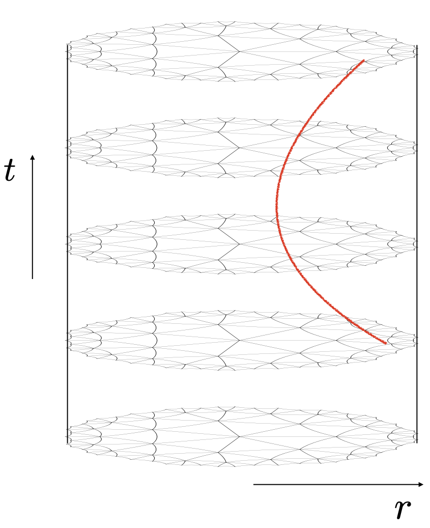
Figure 3: A general bulk geodesic between two points bends into the bulk due to the time dilation of the coefficient $g_{00}(\rho)$ in the metric (2.3) when moving toward the boundary of the AdS₃ cylinder.

4 The free theory

Since the free theory in the continuum has a simple analytical solution, we use it to check the fidelity of our lattice discretization and the convergence of the Monte Carlo simulation. For a given mass-squared $m^{2}$, the analytic bulk Green’s function $G_{bb}(X,X^{\prime})$ between two points $X$ and $X^{\prime}$ in AdS_d+1 is the solution to the equation

$$(-\nabla^{2}+m^{2})G=\frac{1}{\sqrt{g}}\delta^{d+1}(X-X^{\prime})\;.$$ (4.1)

Here $\nabla_{\mu}$ is the covariant derivative and $\nabla^{2}=\nabla_{\mu}\nabla^{\mu}=\frac{1}{\sqrt{g}}\partial_{\mu}\sqrt{g}g^{\mu\nu}\partial_{\nu}$ is the Laplace operator. The Green’s function is given by Burgess:1984ti ; Hijano:2015zsa

$$G_{bb}(\sigma(X,X^{\prime}))=e^{-\Delta\sigma}{}_{2}F_{1}\bigg{(}\Delta,\frac{d}{2},\Delta+1-\frac{d}{2};e^{-2\sigma}\bigg{)}\;,$$ (4.2)

where $\sigma$ is the geodesic between $X$ and $X^{\prime}$ and the scaling dimension is related to the mass through $m^{2}\ell^{2}=\Delta(\Delta-d)$ with $\ell$ being the AdS radius. For $d=2$ the bulk Green’s function in AdS₃ has the simple closed form

$$G_{bb}(\sigma)=\frac{e^{-\Delta\sigma}}{1-e^{-2\sigma}}\;,$$ (4.3)

with the geodesic distance given by

$$\cosh(\sigma)=\cosh(t-t^{\prime})\cosh(\rho)\cosh(\rho^{\prime})-\sinh(\rho)\sinh(\rho^{\prime})\cos(\theta-\theta^{\prime})\;$$ (4.4)

in global hyperbolic coordinates (2.5). The free discretized Green’s function equation (4.1) satifies the matrix equation $M_{xt,\tilde{x}\tilde{t}}\,G(\tilde{x},\tilde{t};x_{0},t_{0})=\delta_{x,x_{0}}\delta_{t,t_{0}}$ :

$$\sum_{y\in\langle x,y\rangle}\frac{1}{2}(\sqrt{g^{x}_{00}} + \sqrt{g^{y}_{00}})(G(x,t;x_{0},t_{0})-G(y,t;x_{0},t_{0}))+m^{2}_{0}\sqrt{g^{x}_{00}}G(x,t;x_{0},t_{0})$$

$$+ \frac{1}{\sqrt{g^{x}_{00}}}(2G(x,t;x_{0},t_{0})-G(x,t+1;x_{0},t_{0})-G(x,t-1;x_{0},t_{0}))=\delta_{x,x_{0}}\delta_{t,t_{0}}\;,$$

where $\sqrt{g^{x}_{00}}=\cosh(\rho_{x})$. This is equivalent to the Gaussian path integral $\langle\phi(t,x)\phi(t_{0},x_{0})\rangle\equiv G(x,t;x_{0},t_{0})$, allowing us to check the Monte Carlo convergence against the exact the matrix inverse $M^{-1}$ at $\lambda_{0}=0$.

For the massless case, we compute the lattice propagator $G_{\tilde{x}\tilde{t},x_{0}t_{0}}\equiv G(\tilde{x},\tilde{t};x_{0},t_{0})$ via matrix inversion and compare it with the form of the analytic propagator $G_{bb}$. We compute the lattice propagator betweean all lattice points, as well as between only pairs of points with zero temporal or spatial separation. To avoid boundary effects, the $L^{\text{th}}$ layer is not included in measurements. We check the Klebanov-Witten form $m^{2}\ell^{2}=\Delta(\Delta-d)$ from holography. The results are shown in Fig. 4 and show good agreement with the expected value of $\Delta=2$ for the massless case. We note that similar to AdS₂ in Asaduzzaman_2020 , there is a small mass renormalization yielding an effective mass $m^{2}>0$ and a slightly larger scale, $\Delta>2$.

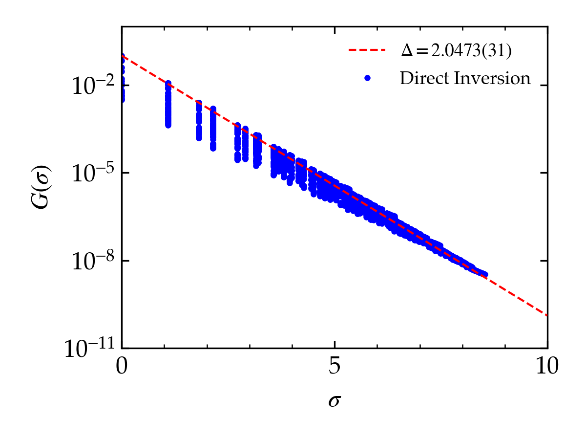
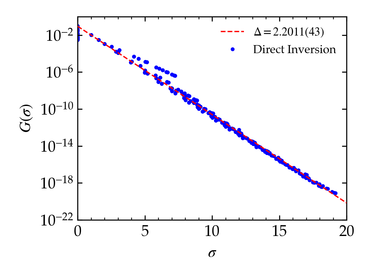
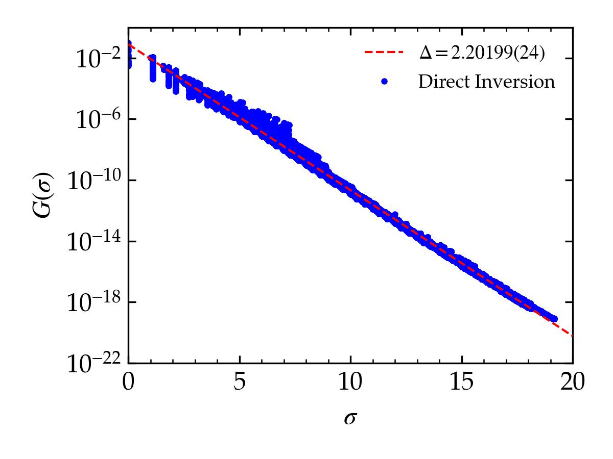
Figure 4: Checks in the non-interacting regime of the AdS₃ lattice realization from a direct inversion of the massless Green’s function $G_{bb}(\sigma)$ for $L=4$. Top left: The propagator for all pairs of points with zero temporal separation (i.e. pairs of points in the same time slice). Top right: The propagator for all pairs of points with zero spatial separation. Bottom: All-to-all propagator.

In Fig. 5 we compare the propagators from direct inversion to measurements from a Monte Carlo simulation of the same lattice. We see good agreement for all measurements larger than the statistical error in the Monte Carlo data, which is of order $10^{-6}$.

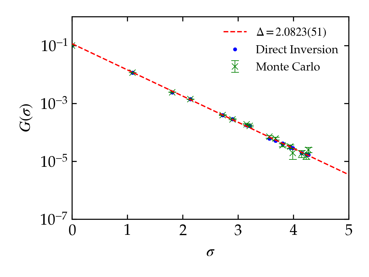
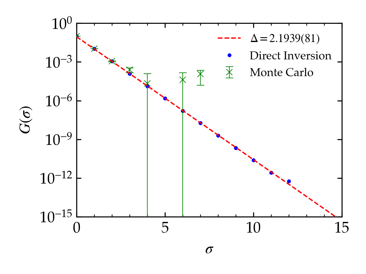
Figure 5: Checks between the direct inversion and Monte Carlo for propagators for the massless case with $L=4$. All of the fits shown are from the direct inversion data. Left: Propagator from the center point to all other spatial points on the same time slice. Right: Propagator along the center axis of the cylinder to all other temporal center points.

5 The interacting theory

To go beyond the free theory of Sec. 4 we use the action (3.1) with $\lambda_{0}\neq 0$. We are specifically interested in determining if our lattice supports a critical point. This is the first step in being able to eventually determine what type of CFT is produced on the boundary at criticality.

5.1 The $\phi^{4}$ critical point

To study the theory (3.1) with non-zero $\lambda_{0}$ and tachyonic mass $\mu_{0}^{2}=-m_{0}^{2}$, we perform a lattice Monte Carlo simulation using a combination of Metropolis Metropolis1953Equation , overrelaxation overrelax , and the Brower-Tamayo cluster algorithm Brower:1989mt with single cluster Wolff updates wolff . The critical point will depend on the two parameters, $\lambda_{0}$ and $\mu_{0}^{2}$, so we set $\lambda_{0}=1$ and sweep over $\mu_{0}^{2}$ values to find the critical $\mu^{2}_{c}$, which we define below. We repeat this process for an increasing number of lattice layers. For each lattice size we choose the number of time slices $N_{t}$ to be equal to the number of points on the outermost spatial layer $L$ so that the lattice boundary has $N^{2}_{t}$ points.

To analyze the critical behavior of the theory we measure two bulk quantities: the magnetic susceptibility $\chi$ and the Binder cumulant BINDER198879 . The magnetic susceptibility $\chi$ is defined as

$$\chi=\dfrac{1}{V}\left(\langle m^{2}\rangle-\langle|m|\rangle^{2}\right)\;,$$ (5.1)

where we have introduced the lattice volume $V=N_{t}\sum_{x}\cosh\rho_{x}$ and the magnetization $m=\sum_{x,t}\cosh\rho_{x}\phi_{x,t}$. At a second-order phase transition we expect to see a peak in the susceptibility that grows with the lattice volume. The 4th-order Binder cumulant $U_{4}$,

$$U_{4}=\dfrac{3}{2}\left(1-\dfrac{\langle m^{4}\rangle}{3\langle m^{2}\rangle^{2}}\right)\;,$$ (5.2)

serves to determine whether the system is in the disordered phase $(U_{4}=0)$ or the ordered phase ($U_{4}=1$). At a second-order phase transition, we expect the Binder cumulant to approach a step function at the critical temperature as the lattice volume goes to infinity.

We perform a finite-size scaling analysis fisher ; landau ; BINDER198879 by scaling $\chi$ and $T$ by powers of the volume, $V^{y_{\chi}}$ and $V^{y_{T}}$, respectively. We then adjust the exponents $y_{\chi}$ and $y_{T}$ so that the data for the different lattice sizes collapses onto a single curve, as shown in Fig. 6. The observed behavior is clear evidence of a second-order phase transition. We note that the traditional finite-size scaling formalism is designed for uniform lattices in flat space, and without a careful discussion of finite size scaling in hyperbolic space we do not attempt to relate this scaling to conventional critical exponents for either a bulk transition or a transition for a CFT at the boundary. Indeed, since a large fraction of the total number of lattice sites are on the last layer at $\rho\simeq\rho_{\text{max}}$, distinguishing between bulk and boundary criticality may be difficult at best; they may well be tied to each other as a consequence of the AdS/CFT correspondence. We defer to a later work the study of scaling for correlators and the goal to find the proper finite-size formalism for AdS space.

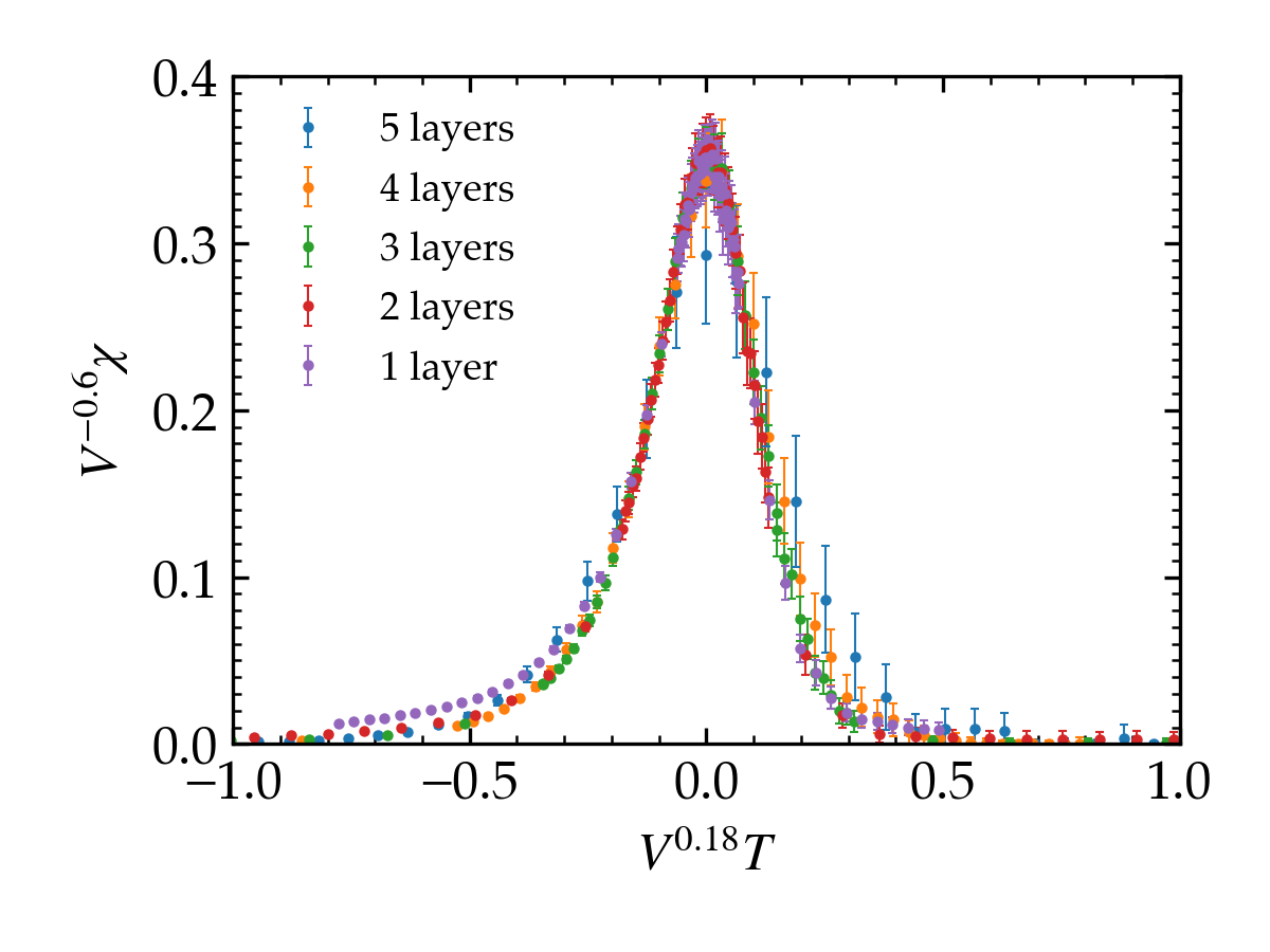
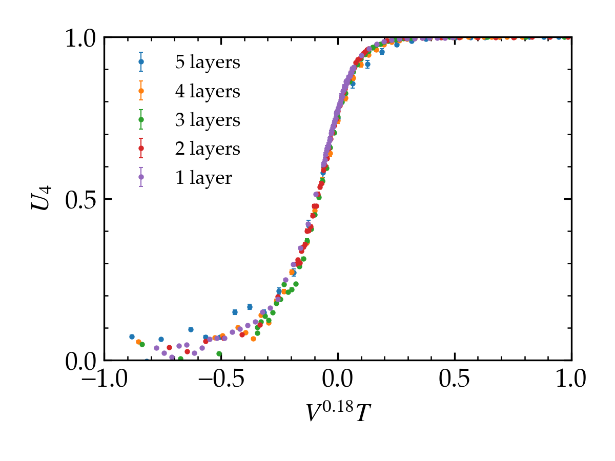
Figure 6: Evidence for a second order phase transition for bulk $\phi^{4}$ theory in the Euclidean AdS₃ cylinder at $\lambda_{0}=1$. Left: The magnetic susceptibility $\chi$. Right: The 4th-order Binder cumulant $U_{4}$. We have scaled $\chi$ and $T$ by the lattice volume raised to an exponent, with the exponents chosen so that the data collapses onto a single curve.

We contrast the present discussion with the very interesting investigation in Breuckmann_2020 on the critical Ising model in hyperbolic space with periodic boundary conditions. With periodic boundary conditions, these hyperbolic triangulations on closed Riemann manifolds in 2D are the analogue of the Platonic solids on spheres for genus $g=0$ and the finite triangulated torus for genus $g=1$. For Riemann surfaces at higher genus ($g>1$), the finite equilateral triangulations correspond to negative curvature manifolds. The smallest classic example is the famous $g=3$ Klein quartic Klein triangulated by 56 $(2,3,7)$ equilateral triangles with 168 proper symmetries. Remarkably, this is the first in an infinite sequence of larger volumes and higher genuses Sausset_2007 .

Given the highly connected graph as the genus increases, it is not surprising to find critical behavior with mean field exponents as in Breuckmann_2020 . This paper also finds mean field exponents for the 3D hyperbolic Ising lattice with periodic boundary conditions. Moreover, periodic boundary conditions are interesting for applications to interacting particles in physical systems and necessary for experimentally realizing toric codes for quantum computing. Nonetheless, this investigation Breuckmann_2020 can not be directly compared with the critical properties seen in Fig. 6 on our AdS tessellation approaching the hyperbolic surface with Dirichlet boundary conditions at infinity. Instead this article focuses on the AdS/CFT correspondence with the goal to understand the non-perturbative relation between bulk and boundary critical behavior.

6 Discussion

Adapting the power of Euclidean lattice field theory to AdS space offers new possibilities for exploring strongly coupled phenomena. In this article we choose the simplest case of scalar $\phi^{4}$ theory. However, by implementing the simplicial construction advocated in the Quantum Finite Element framework brower2021PoS , we believe general field theories, including fermions Brower:2016vsl ; Catterall:2018dns and gauge fields Christ:1982ck coupled to each other or to scalars, can be realized on any smooth Riemann manifold. By constructing the lattice for AdS₃ in a Euclidean cylinder geometry, we are able to foliate time with spatial sections on the Poincaré disk ${\mathbb{H}}^{2}$ using the triangle group Brower:2019kyh , which is a discrete subgroup of the full conformal group. The triangle group fixes the bulk UV lattice cut-off but the finite lattice volume imposes an arbitrary center point breaking the discrete isometries of AdS space. However, due the IR/UV connection of the AdS/CFT correspondence, the IR cutoff $\rho_{\text{max}}$ implies an exponentially small UV cut-off $\epsilon\sim\exp(-\rho_{\text{max}})$ for the boundary CFT. This raises the intriguing possibility of convergence to a continuum boundary CFT that does not require UV completion in the bulk – perhaps an echo of the basic concept of holography for gauge/gravity duality.

We checked the free theory propagators using both direct matrix inversion as well as Monte Carlo methods and see scaling consistent with the continuum theory. By looking at the magnetic susceptibility and the Binder cumulant we found strong evidence that there is a bulk critical point for $\phi^{4}$ theory on our AdS₃ lattice. Further simulations of the correlators are ongoing to understand the subtleties of the phase transition and to determine the approach to the CFT boundary (2.8). We seek to relate our finite volume scaling result to local operators as well as address the issue of the nature of the boundary CFT and whether it is a short- or long-range Ising model Paulos:2016 ; Behan:2017emf , or something else. To determine the scaling exponents requires more precision, but this is easily achieved. With efficient cluster algorithms Brower:1989mt , high statistics Monte Carlo simulations for $\phi^{4}$ theory on lattice volumes up to $\mathcal{O}(10^{6})$ sites are feasible. Comparison with Table 1 implies that lattices exceeding $L=8$ with a number of time slices on the order of $N(L)$ are reasonable. These methods naturally apply to the Ising model, which is presumably universally equivalent to $\phi^{4}$ theory approaching the transition.

Another feature of our lattice is to introduce the Hamiltonian operator in Euclidean AdS space. For the Ising representation we can treat time exactly using continuous time loop algorithms Beard:1996wj . For both AdS₃ and AdS₂ the Ising Hamiltonian takes the conventional form

$$\hat{H}_{\mathrm{AdS}}=-\sum_{i}\cosh(\rho_{i})\sigma^{x}_{i}-t\sum_{\langle ij\rangle}\cosh(\rho_{i})\sigma^{z}_{i}\sigma^{z}_{j}\;,$$ (6.1)

where the sum is over the transverse spatial links. For AdS₃ the boundary at $\rho=\rho_{\max}$ is topologically a circle ${\mathbb{S}}^{1}$ with $\theta\in[-\pi,\pi)$. For AdS₂ this topology is even simpler: it is a strip (2.7), reminiscent of open strings but with 1D conformal quantum mechanics at each end: $\theta=0,\pi$. This geometry is amenable to many analytical methods as highlighted in Hogervorst:2021spa . It is also the simplest geometry in which to calculate bulk and boundary phenomena in the presence of differing boundary conditions Cogburn:2021awx . So both Hamiltonian AdS₃ and AdS₂ are ideal test systems.

The dynamics of the Ising model in hyperbolic space are more interesting and less well understood than in flat space, but even the classical Ising model on $\mathbb{H}^{2}$ is interesting Krcmar:2008 ; Shima:2005vq ; Asaduzzaman:2021bcw . Here the $K_{ij}$ weights for the regular triangle group lattice are constant, so in principle there is no need for counterterms to restore the isometries at a second order phase transition. We note that in (1+2)-dimensions we can use the Hamiltonian to go to Minkowski space and study unitary time evolution $U(t)=\exp(-it\hat{H})$ suited to quantum computing. One approach is to simulate this on a digital quantum computer with the standard Trotter expansion. An intriguing alternative is specific hardware being introduced Koll_r_2019 ; Bienias:2021lem ; Boettcher:2019xwl ; Yu:2020 ; Kollar:2019 that purports to realize the discrete $\mathbb{H}^{2}$ lattice.

Finally, time evolution for gravity is an interesting and challenging problem. Recently in Ref. Cotler:2022weg , similar finite element methods (FEM) were introduced in Minkowski space to address the interesting problem of unitarity in an expanding universe. However, to enter the realm of gravity in our context requires dynamical metric fluctuations for bulk gravity dual to a boundary CFT with a conserved energy momentum tensor. A natural framework is causal Regge calculus allowing for a change in the simplicial geometry Catterall:2018dns . With our construction a first step is to consider weak gravitational fluctuations around a fixed curved manifold by allowing the bonds to fluctuate. This is yet another possible extension of this modest proposal in utilizing lattice field theory in an AdS background.

References

- (1) C. G. Callan, Jr. and F. Wilczek, “INFRARED BEHAVIOR AT NEGATIVE CURVATURE,” Nucl. Phys. B 340 (1990) 366–386.
- (2) R. Rattazzi, V. S. Rychkov, E. Tonni, and A. Vichi, “Bounding scalar operator dimensions in 4D CFT,” JHEP 12 (2008) 031, arXiv:0807.0004 [hep-th].
- (3) S. El-Showk, M. F. Paulos, D. Poland, S. Rychkov, D. Simmons-Duffin, and A. Vichi, “Solving the 3D Ising Model with the Conformal Bootstrap,” Phys. Rev. D 86 (2012) 025022, arXiv:1203.6064 [hep-th].
- (4) B. Joó, C. Jung, N. H. Christ, W. Detmold, R. G. Edwards, M. Savage, and P. Shanahan, “Status and future perspectives for lattice gauge theory calculations to the exascale and beyond,” The European Physical Journal A 55 no. 11, (2019) 199. https://doi.org/10.1140/epja/i2019-12919-7.
- (5) R. C. Brower, E. S. Weinberg, G. T. Fleming, A. D. Gasbarro, T. G. Raben, and C.-I. Tan, “Lattice Dirac Fermions on a Simplicial Riemannian Manifold,” Phys. Rev. D95 no. 11, (2017) 114510, arXiv:1610.08587 [hep-lat].
- (6) R. C. Brower, M. Cheng, E. S. Weinberg, G. T. Fleming, A. D. Gasbarro, T. G. Raben, and C.-I. Tan, “Lattice field theory on Riemann manifolds: Numerical tests for the 2-d Ising CFT on ,” Phys. Rev. D98 no. 1, (2018) 014502, arXiv:1803.08512 [hep-lat].
- (7) R. C. Brower, G. T. Fleming, A. D. Gasbarro, D. Howarth, T. G. Raben, C.-I. Tan, and E. S. Weinberg, “Radial lattice quantization of 3D 4 field theory,” Phys. Rev. D 104 no. 9, (2021) 094502, arXiv:2006.15636 [hep-lat].
- (8) R. C. Brower, E. S. Weinberg, G. T. Fleming, A. D. Gasbarro, T. G. Raben, and C.-I. Tan, “Prospects for lattice qfts on curved riemann manifolds,” PoS, LATTICE2021 (2021) .
- (9) R. C. Brower, C. V. Cogburn, A. L. Fitzpatrick, D. Howarth, and C.-I. Tan, “Lattice Setup for Quantum Field Theory in AdS2,” arXiv:1912.07606 [hep-th].
- (10) M. F. Paulos, J. Penedones, J. Toledo, B. C. van Rees, and P. Vieira, “The S-matrix bootstrap. Part I: QFT in AdS,” JHEP 11 (2017) 133, arXiv:1607.06109 [hep-th].
- (11) M. F. Paulos, J. Penedones, J. Toledo, B. C. van Rees, and P. Vieira, “The S-matrix bootstrap II: two dimensional amplitudes,” JHEP 11 (2017) 143, arXiv:1607.06110 [hep-th].
- (12) S. Rychkov and L. G. Vitale, “Hamiltonian truncation study of the theory in two dimensions. II. The -broken phase and the Chang duality,” Phys. Rev. D 93 no. 6, (2016) 065014, arXiv:1512.00493 [hep-th].
- (13) M. Hogervorst, M. Meineri, J. Penedones, and K. S. Vaziri, “Hamiltonian truncation in Anti-de Sitter spacetime,” arXiv:2104.10689 [hep-th].
- (14) N. Anand, E. Katz, Z. U. Khandker, and M. T. Walters, “Nonperturbative dynamics of (2+1)d -theory from Hamiltonian truncation,” JHEP 05 (2021) 190, arXiv:2010.09730 [hep-th].
- (15) E. Katz, Z. U. Khandker, and M. T. Walters, “A Conformal Truncation Framework for Infinite-Volume Dynamics,” JHEP 07 (2016) 140, arXiv:1604.01766 [hep-th].
- (16) N. Anand, A. L. Fitzpatrick, E. Katz, Z. U. Khandker, M. T. Walters, and Y. Xin, “Introduction to Lightcone Conformal Truncation: QFT Dynamics from CFT Data,” arXiv:2005.13544 [hep-th].
- (17) I. Bengtsson, “Anti-de Sitter Space,”. http://3dhouse.se/ingemar/relteori/Kurs.pdf.
- (18) E. Witten, “Anti-de Sitter space and holography,” Adv. Theor. Math. Phys. 2 (1998) 253–291, arXiv:hep-th/9802150.
- (19) D. Berenstein and D. Grabovsky, “The tortoise and the hare: a causality puzzle in ads/cft,” Classical and Quantum Gravity 38 no. 10, (Apr, 2021) 105008. http://dx.doi.org/10.1088/1361-6382/abf1c7.
- (20) M. Asaduzzaman, S. Catterall, J. Hubisz, R. Nelson, and J. Unmuth-Yockey, “Holography on tessellations of hyperbolic space,” Physical Review D 102 no. 3, (Aug, 2020) . http://dx.doi.org/10.1103/PhysRevD.102.034511.
- (21) G. Strang and G. Fix, An Analysis of the Finite Element Method 2nd Edition. Wellesley-Cambridge, 2nd ed., 5, 2008. http://amazon.com/o/ASIN/0980232708/.
- (22) B. B. Beard and U. J. Wiese, “Simulations of discrete quantum systems in continuous Euclidean time,” Phys. Rev. Lett. 77 (1996) 5130–5133, arXiv:cond-mat/9602164.
- (23) C. P. Burgess and C. A. Lutken, “Propagators and Effective Potentials in Anti-de Sitter Space,” Phys. Lett. B 153 (1985) 137–141.
- (24) E. Hijano, P. Kraus, E. Perlmutter, and R. Snively, “Witten Diagrams Revisited: The AdS Geometry of Conformal Blocks,” JHEP 01 (2016) 146, arXiv:1508.00501 [hep-th].
- (25) N. Metropolis, A. W. Rosenbluth, M. N. Rosenbluth, A. H. Teller, and E. Teller, “Equation of state calculations by fast computing machines,” Journal of Chemical Physics 21 no. 6, (1953) 1087–1092.
- (26) S. L. Adler, “Over-relaxation method for the monte carlo evaluation of the partition function for multiquadratic actions,” Phys. Rev. D 23 (Jun, 1981) 2901–2904. https://link.aps.org/doi/10.1103/PhysRevD.23.2901.
- (27) R. Brower and P. Tamayo, “Embedded Dynamics for Theory,” Phys.Rev.Lett. 62 (1989) 1087–1090.
- (28) U. Wolff, “Collective monte carlo updating for spin systems,” Phys. Rev. Lett. 62 (Jan, 1989) 361–364. https://link.aps.org/doi/10.1103/PhysRevLett.62.361.
- (29) K. Binder, “Finite size scaling analysis of ising model block distribution functions,” in Finite-Size Scaling, J. L. CARDY, ed., vol. 2 of Current Physics–Sources and Comments, pp. 79–100. Elsevier, 1988. https://www.sciencedirect.com/science/article/pii/B9780444871091500121.
- (30) M. E. Fisher and M. N. Barber, “Scaling theory for finite-size effects in the critical region,” Phys. Rev. Lett. 28 (Jun, 1972) 1516–1519. https://link.aps.org/doi/10.1103/PhysRevLett.28.1516.
- (31) D. P. Landau, “Finite-size behavior of the simple-cubic ising lattice,” Phys. Rev. B 14 (Jul, 1976) 255–262. https://link.aps.org/doi/10.1103/PhysRevB.14.255.
- (32) N. P. Breuckmann, B. Placke, and A. Roy, “Critical properties of the ising model in hyperbolic space,” Physical Review E 101 no. 2, (Feb, 2020) . http://dx.doi.org/10.1103/PhysRevE.101.022124.
- (33) F. Klein and R. Fricke, Vorlesungen Uber Die Theorie for Elliptischen Modulfunctionen. Teuber, Leipzig, 1890.
- (34) F. Sausset and G. Tarjus, “Periodic boundary conditions on the pseudosphere,” Journal of Physics A: Mathematical and Theoretical 40 no. 43, (Oct, 2007) 12873–12899. https://doi.org/10.1088/1751-8113/40/43/004.
- (35) S. Catterall, J. Laiho, and J. Unmuth-Yockey, “Kähler-Dirac fermions on Euclidean dynamical triangulations,” Phys. Rev. D 98 no. 11, (2018) 114503, arXiv:1810.10626 [hep-lat].
- (36) N. H. Christ, R. Friedberg, and T. D. Lee, “Gauge theory on a random lattice,” Nucl. Phys. B210 (1982) 310.
- (37) M. F. Paulos, S. Rychkov, B. C. van Rees, and B. Zan, “Conformal invariance in the long-range ising model,” Nuclear Physics B 902 (Jan, 2016) 246–291. http://dx.doi.org/10.1016/j.nuclphysb.2015.10.018.
- (38) C. Behan, L. Rastelli, S. Rychkov, and B. Zan, “A scaling theory for the long-range to short-range crossover and an infrared duality,” J. Phys. A 50 no. 35, (2017) 354002, arXiv:1703.05325 [hep-th].
- (39) C. V. Cogburn, “CFT2 in the Bulk,” arXiv:2110.04303 [hep-th].
- (40) R. Krcmar, A. Gendiar, K. Ueda, and T. Nishino, “Ising model on a hyperbolic lattice studied by the corner transfer matrix renormalization group method,” Journal of Physics A: Mathematical and Theoretical 41 no. 12, (Mar, 2008) 125001. http://dx.doi.org/10.1088/1751-8113/41/12/125001.
- (41) H. Shima and Y. Sakaniwa, “Geometric effects on critical behaviours of the Ising model,” J. Phys. A 39 (2006) 4921, arXiv:cond-mat/0511539.
- (42) M. Asaduzzaman, S. Catterall, J. Hubisz, R. Nelson, and J. Unmuth-Yockey, “Holography for Ising spins on the hyperbolic plane,” arXiv:2112.00184 [hep-lat].
- (43) A. J. Kollár, M. Fitzpatrick, and A. A. Houck, “Hyperbolic lattices in circuit quantum electrodynamics,” Nature 571 no. 7763, (Jul, 2019) 45–50. http://dx.doi.org/10.1038/s41586-019-1348-3.
- (44) P. Bienias, I. Boettcher, R. Belyansky, A. J. Kollar, and A. V. Gorshkov, “Circuit Quantum Electrodynamics in Hyperbolic Space: From Photon Bound States to Frustrated Spin Models,” Phys. Rev. Lett. 128 no. 1, (2022) 013601, arXiv:2105.06490 [quant-ph].
- (45) I. Boettcher, P. Bienias, R. Belyansky, A. J. Kollár, and A. V. Gorshkov, “Quantum Simulation of Hyperbolic Space with Circuit Quantum Electrodynamics: From Graphs to Geometry,” Phys. Rev. A 102 no. 3, (2020) 032208, arXiv:1910.12318 [quant-ph].
- (46) S. Yu, X. Piao, and N. Park, “Topological hyperbolic lattices,” Physical Review Letters 125 no. 5, (Jul, 2020) . http://dx.doi.org/10.1103/PhysRevLett.125.053901.
- (47) A. J. Kollár, M. Fitzpatrick, P. Sarnak, and A. A. Houck, “Line-graph lattices: Euclidean and non-euclidean flat bands, and implementations in circuit quantum electrodynamics,” Communications in Mathematical Physics 376 no. 3, (Dec, 2019) 1909–1956. http://dx.doi.org/10.1007/s00220-019-03645-8.
- (48) J. Cotler and A. Strominger, “The Universe as a Quantum Encoder,” arXiv:2201.11658 [hep-th].