Probing emergent QED in quantum spin ice via Raman scattering of phonons:
shallow inelastic scattering and pair production

Abstract

We present a new mechanism for Raman scattering of phonons, which is based on the linear magnetoelastic coupling present in non-Kramers magnetic ions. This provides a direct coupling of Raman-active phonons to the magnet’s quasiparticles. We propose to use this mechanism to probe the emergent magnetic monopoles, electric charges, and photons of the emergent quantum electrodynamics (eQED) of the U(1) quantum spin liquid known as quantum spin ice. Detecting this eQED in candidate rare-earth pyrochlore materials, or indeed signatures of topological magnetic phases more generally, is a challenging task. We show that the Raman scattering cross-section of the phonons directly yields relevant information, with the broadening of the phonon linewidth, which we compute, exhibiting a characteristic frequency dependence reflecting the two-particle density of states of the emergent excitations. Remarkably, we find that the Raman linewidth is sensitive to the details of the symmetry fractionalisation and hence can reveal information about the projective implementation of symmetry in the quantum spin liquid, thereby providing a diagnostic for a $\pi$-flux phase. The Raman scattering of the phonons thus provides a useful experimental tool to probe the fractionalisation in quantum spin liquids that turns out closely to mirror pair production in quantum electrodynamics and the deep inelastic scattering of quantum chromodynamics. Indeed, the difference to the latter is conceptual more than technical: the partons (quarks) emerge from the hadrons at high energies due to asymptotic freedom, while those in eQED arise from fractionalisation of the spins at low energies.

I Introduction

The long-range entanglement present in quantum spin liquids (QSLs) lead to novel low-energy quasi-particles with fractionalised quantum numbers [anderson1987resonating, anderson1973resonating, PhysRevLett.86.1881, wen2002quantum, kitaev2006anyons, balents2010spin, wen2017colloquium, lee2008end, broholm2020quantum, Knolle_ARCMP_2019, takagi2019concept]. Experimental signatures of these fractionalised quasi-particles can provide direct evidence of the underlying entanglement pattern that characterises the quantum order in the QSLs. However, detecting experimental signatures of such unconventional fractionalised excitations calls for an array of complementary experimental probes to collectively provide information about the QSL.

In this context, probing the spins through their coupling to phonons–via magnetoelastic interactions– provides useful spectroscopic insights into the physics of QSLs. An example of this is the ultrasonic attenuation [lee2011, shiralieva2021magnetoelastic, PhysRevResearch.2.033180] and anomalies [rucl32021, PhysRevB.84.041102] of the acoustic phonons in QSLs. Magnetoelastic interactions are also believed to play an important role in the large thermal Hall response observed in several correlated insulators including the pseudo-gap phase of lightly doped cuprates [grissonnanche2019giant] and the magnetic-field induced paramagnetic phase of the honeycomb magnet $\alpha$-RuCl${}_{3}$ [kasahara2018unusual, nasu2016fermionic, banerjee2016proximate, banerjee2017neutron, PhysRevLett.121.147201, vinkler2018approximately, kasahara2018majorana, yamashita2020sample, yokoi2021half, czajka2021oscillations].

A related probe for the spin physics are optical phonons, via infrared and Raman scattering experiments where phonon energy and linewidth encode such effects [pal2020probing, rucl32021, sandilands, LiIrO32016, satoru, natalia2021]. Notably, such phonon spectroscopy can sensitively detect magnetic, superconducting, or charge-density wave ordering, as well as couples to the resultant low-energy quasi-particles in these conventional phases [luthi2007physical, toth2016electromagnon, aynajian2008energy]. In the simplest QSLs, however, symmetries are not spontaneously [anderson1973resonating] broken and the nature of phonon renormalisation, at low temperatures, is governed by the properties of fractionalised excitations of the QSLs which provide additional scattering channels for the phonons. This is expected, in particular, to lead to an anomalous broadening of the phonon linewidth at low temperatures whose characterisation can then reveal important information regarding the QSL excitations.

The spin-phonon effects are expected to be particularly strong in spin-orbit coupled magnets where the magnetic moment is sensitive to the real space geometry due to an interlocking of spin and real space [bhattacharjee2012spin, witczak2014correlated, NussinovJeroenRMP, HKK_kitaev]. Indeed such spin-phonon coupling has recently been explored both experimentally and theoretically in candidate Kitaev QSLs such as $\alpha$-RuCl${}_{3}$ [rucl32021, metavitsiadis2021optical, nasu2016fermionic], Cu${}_{2}$IrO${}_{3}$ [pal2020probing], $\beta$- and $\gamma$-Li${}_{2}$IrO${}_{3}$ [LiIrO32016, PhysRevB.92.094439] etc. In particular, for Cu${}_{2}$IrO${}_{3}$ [pal2020probing], the anomalous broadening of the phonon peaks and frequency softening at low temperatures is accounted for by the low-energy Majorana fermions that the spin fractionalises into [kitaev2006anyons].

Another equally interesting family of spin-orbit coupled frustrated magnets are obtained in the rare-earth pyrochlores with magnetic moments sitting on a three-dimensional network of corner sharing tetrahedra, leading to frustrated spin-spin interactions. These so-called spin ice systems [BramwellGingras2001, castelnovo2012, gingrass2014, rau, bramwell2020, ramirez1999zero, PhysRevLett.79.2554, erfanifam, yb2016, RevModPhys.82.53, PhysRevB.93.064406, PhysRevLett.119.057203, PhysRevX.1.021002, gingrass2014, PhysRevLett.109.097205, PhysRevB.87.184423, kimura, prhfo, tbtioprincep, HoTbDy, ruminy2014, HoTbDy] are primary candidates to realise both classical cooperative paramagnets [MoessnerChalker98, chalker, PhysRevB.71.014424, henley2010coulomb] as well as QSLs [hermele, ramandimer2005, PhysRevLett.91.167004, gingrass2014, savary, sungbin2012, PhysRevLett.108.067204, benton, PhysRevLett.100.047208, PhysRevLett.112.167203, PhysRevB.92.144417, chang2012higgs, PhysRevLett.115.077202]. The magnetic moments result from a very intricate interplay of inter-orbital Coulomb repulsion, atomic spin-orbit coupling, and crystal field effects.

A rather extreme example of interplay between several competing interactions is seen in an interesting subset among the pyrochlores which are the so-called non-Kramers spin ice materials such as Pr${}_{2}$Zr${}_{2}$O${}_{7}$ [kimura, satoru, PhysRevB.94.165153], Pr${}_{2}$Hf${}_{2}$O${}_{7}$ [prhfo], Tb${}_{2}$Ti${}_{2}$O${}_{7}$ [tbtioprincep, HoTbDy, ruminy2014], Ho${}_{2}$Ti${}_{2}$O${}_{7}$ [HoTbDy] etc. In these pyrochlore magnets, the low-energy spin-1/2 magnetic moments arise from even-electron wave functions [PZO_doublet, tbtioprincep, HoTbDy]. The degeneracy of such a non-Kramers doublet is protected by lattice symmetry, the $D_{3d}$ symmetry at the pyrochlore lattice site, instead of the usual time reversal symmetry for Kramers doublets. Therefore under time reversal symmetry, $\mathcal{T}$, the transformation of the low-energy doublets, $s^{\alpha}$ ($\alpha=x,y,z$), made out of spin-orbit coupled wave functions is given by

$$\mathcal{T}~{}:~{}\{s^{x},s^{y},s^{z}\}\rightarrow\{s^{x},s^{y},-s^{z}\}$$ (1)

This is in stark difference from the usual Kramers case as realised in, e.g., Dy${}_{2}$Ti${}_{2}$O${}_{7}$ among others, where all the components of the resultant spin-1/2 are odd under time reversal.

The non-trivial implementation of time reversal symmetry as in Eq. 1 opens up the possibility of using experimental probes which are complementary to the conventional ones. For example, the transformation in Eq. 1 immediately suggests that the transverse components $\{s^{x},s^{y}\}$ can linearly couple to the lattice vibrations of the appropriate space-group symmetry (see Eq. 6 and 7) such that this linear coupling makes the above materials ideal candidates to explore the spin physics through the spin-phonon coupling in vibrational IR/Raman spectroscopy of the relevant phonons. The issue assumes particular importance in the context of QSLs since the spin-spin interactions in several of these non-Kramers pyrochlores, such as Pr${}_{2}$Zr${}_{2}$O${}_{7}$ [Comsatoru], can possibly stabilise a $U(1)$ QSL with gapless emergent photons and gapped bosonic electric and magnetic monopoles [hermele, ramandimer2005, PhysRevLett.91.167004, gingrass2014, savary, sungbin2012, PhysRevLett.108.067204, benton, PhysRevLett.100.047208, PhysRevLett.112.167203, PhysRevB.92.144417, chang2012higgs, PhysRevLett.115.077202]– the so-called Quantum spin ice.

In this paper, we show that indeed such a linear coupling can lead to characteristic experimental signatures of the emergent gauge charges and photons in vibrational Raman spectroscopy of a non-Kramers quantum spin ice, such as those proposed for Pr${}_{2}$Zr${}_{2}$O${}_{7}$. We show that such linear couplings give rise to prominent new interaction channels between the phonon and all the three emergent excitations of the U(1) QSL– the emergent gapped electric and the magnetic charges as well as the gapless photons. These interactions provide new scattering channels for phonons to decay into and lead to an anomalous broadening of the Raman peaks in the low-temperature regime. Remarkably, as we show, such Raman signatures are sensitive to the non-trivial symmetry implementation on the emergent degrees of freedom– the details of the projective representation of the symmetry group [wen2002quantum] under which the low-energy fractionalised excitations of the QSL transform. In particular, in the context of the quantum spin ice, we discuss the two cases of zero and $\pi$-flux. While in the former, the magnetic monopoles do not see any electric flux, in the latter they see an electric $\pi$-flux through every hexagonal plaquette. As a result, the magnetic monopoles in the $\pi$-flux phase transform under the non-trivial magnetic space group, as opposed to the zero-flux phase, with the magnetic monopoles transforming projectively under lattice translation. The resultant effects for both the QSLs are very different from the phonon renormalisation due to anharmonic contributions or magnetic ordering, and hence might present important signatures of the fractionalisation and the emergent gauge field.

It turns out that probing the low-energy fractionalised excitations of the QSL via the Raman/infrared scattering of the phonons is quite similar to– (a) high energy pair production (Fig. 1(a)), and, (b) the deep inelastic scattering [feynman1988behavior, PhysRev.185.1975] of quarks in quantum chromodynamics (QCD) by the leptons as described by the standard model of high-energy particle physics (Fig. 1(b)). The corresponding two relevant vertices are shown side-by-side in Fig. 1(c) and (d) respectively. In QCD, the quarks become asymptotically free at high energies and the high energy lepton can then probe them on sub-hadron length-scales [PhysRevLett.23.930, PhysRevLett.23.935]. In a QSL, however, the non-trivial entanglement leading to fractionalised novel excitations is a low-energy/long-wavelength emergent phenomenon which the phonons can probe via “shallow” inelastic scattering. In particular, we show below while the first of the two processes dominate for the zero-flux QSL, the latter produces important low signatures of the momentum fractionalisation in the $\pi$-flux case. While our work describes such shallow inelastic scattering of an eQED in the context of the quantum spin ices, it readily generalises to other QSLs, and to probe magnetic excitations in quadrupolar systems more broadly.

(a) High energy pair production

(b) Deep Inelastic scattering of hadrons

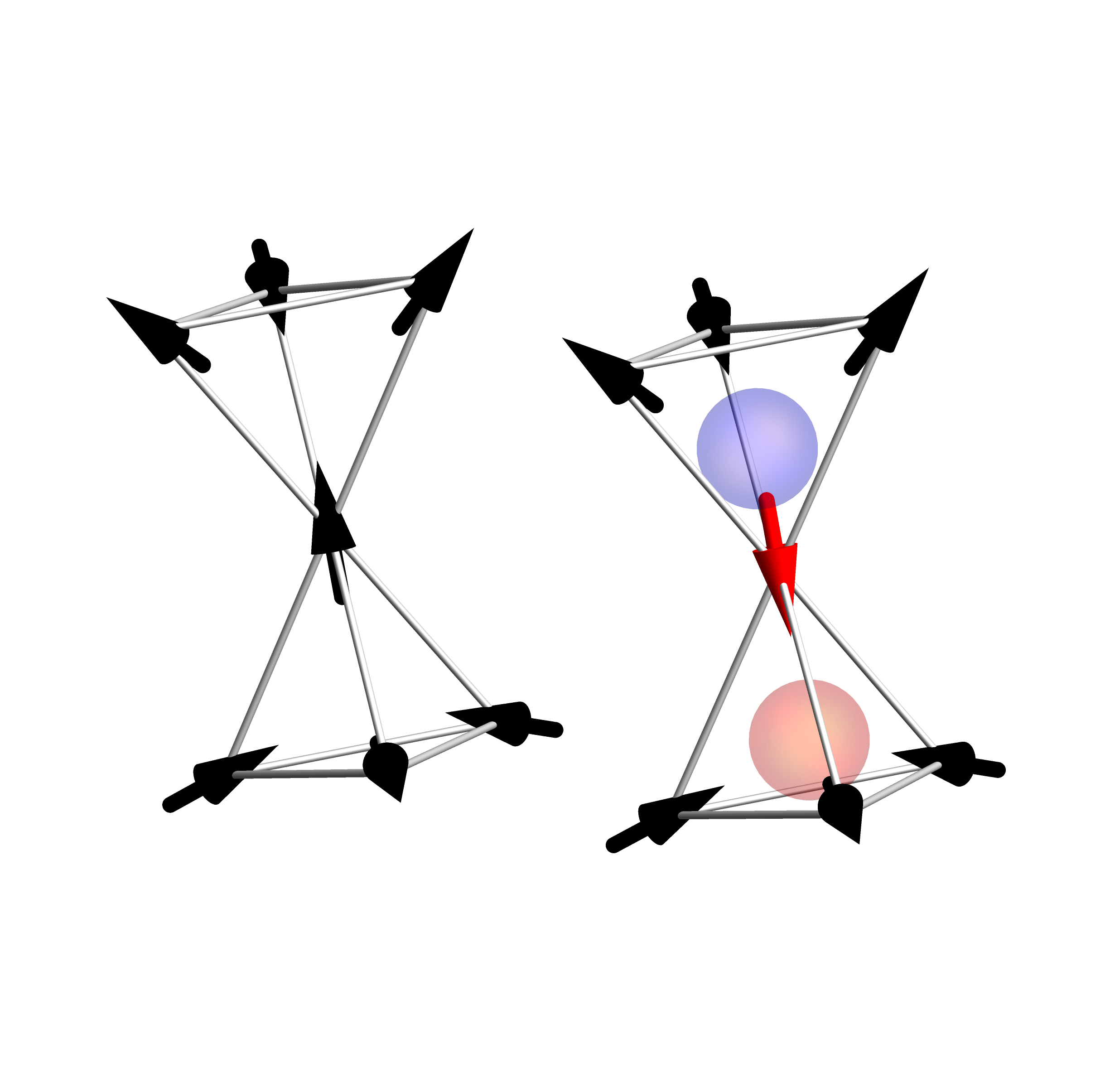
(c) Pair Production in QSL

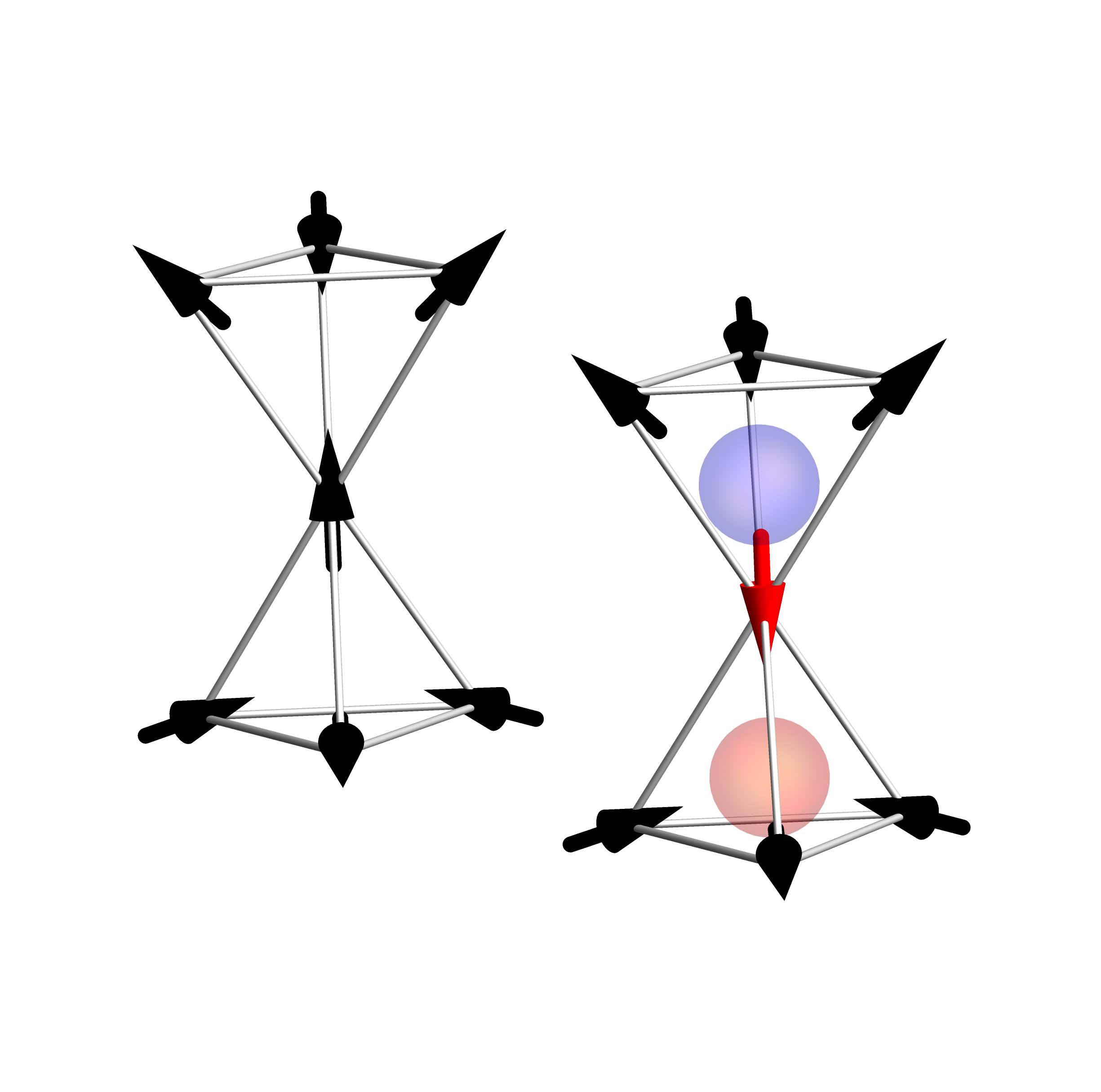
(c) Shallow inelastic scattering in QSI

Figure 1: Correspondence of scattering diagrams: (a) The high energy photon can lead to creation of a positron and an electron via pair production, (b) In deep inelastic scattering, a photon emitted from a lepton scatters off a parton, a quark $q$, contained in the hadron, a $q\bar{q}$-pion as a free particle at high energies, (c) In non-Kramers quantum spin ice, the phonon flips a spin and creates two magnetic monopoles of opposite charges and, (d) In shallow inelastic scattering, an optical phonon emitted from a photon scatters off a parton, a magnetic monopole or electric charge, emerging from the spin degrees of freedom from fractionalisation at low energies.

We note that the above vibrational Raman signatures of the fractionalisation on the phonons are different from the Loudon-Fleury type of Raman scattering where the external photon scatters directly from the charge fluctuation in the Mott insulating phase [shastry, PhysRevLett.113.187201, rau2017, PhysRevB.81.024414, PhysRev.166.514]. This kind of coupling has been explored by Cepas et. al. in the context of Kagome spin liquids [PhysRevB.77.172406], and more pertinent for us, Fu et al. in the context of generic U(1) quantum spin ice [rau2017]. These studies already indicate several anomalous peaks in the Raman intensity profile due to the presence of new scattering channels in the QSL phase invariably indicating magnetic monopoles and gauge excitations of the quantum spin ice. However, due to the localized nature of the 4f-orbitals of Pr${}^{3+}$, the scattering via charge fluctuation is significantly suppressed and the Raman probe mediated by the phonons can then provide dominant signatures of the novel excitations of the U(1) QSL phase in non-Kramers quantum spin ice. In fact, as we show here, even if the phonons are not at resonance with the emergent excitations, the linear magnetoelastic coupling can mediate an effective Loudon-Fleury [PhysRev.166.514, shastry] type of coupling between emergent QSL excitations and the external Raman photons that form the leading contribution in non-Kramers material realisations of quantum spin ice.

We start with a brief overview of our results before delving into the details.

I.1 Overview of the results

The non-Kramers nature of the low-energy doublet in materials such as Pr${}_{2}$Zr${}_{2}$O${}_{7}$ restricts the form of the low-energy spin-spin interactions (Eq. 3) of the non-Kramers doublets as we briefly summarise in Sec. II. A further fallout of the unusual implementation of the time reversal symmetry is that the time reversal-even transverse spin components (Eq. 1) can couple linearly to the Raman active ${\bf e_{g}}$ and ${\bf t_{2g}}$ phonons (Eqs. 6 and 7) as discussed in Sec. III. These linear couplings form the leading order terms that couple the lattice modes with the spins with the latter apparently forming a U(1) QSL state– the quantum spin ice– over a sizeable parameter regime. Sec. IV gives a brief review of this quantum spin ice phase and their fractionalised low-energy excitations– the gapped bosonic electric and magnetic gauge charges and the gapless emergent photons. These excitations are captured via a mean-field description of the parton decomposition of spins leading to a lattice gauge theory. The microscopic couplings of the rare-earth pyrochlore magnets lead to a natural energy-scale separation between the higher energy magnetic sector and lower energy electric sector in quantum spin ice.

Figure 2: Feynman diagrams for the interactions between the excitations of the quantum spin ice and the Raman active phonons in a non-Kramers system due to the linear spin-phonon coupling (Eqs. 6 and 7) : (a) The vertex corresponds to the phonon-magnetic monopole interaction described by Eq. 18 and 19. Dotted, solid and curly line denote phonon, monopole and emergent photon, respectively. Thin and thick solid lines represent two flavours of monopoles, A and B, respectively. (b) Vertex for the phonon-(emergent) photon interaction described by Eq. 24. The circle represents the dipolar form factors (see Eq. 25) that makes the vertex gauge invariant. (c) Vertex for the phonon and electric charge interaction. The dashed line denotes the electric charge.

The partons naturally allow to re-write the linear spin-phonon coupling in terms of the coupling of the phonons with the low-energy excitations of the quantum spin ice. The resultant interaction vertices are shown in Fig. 2 while the details are discussed in Sec. V. In Sec. VI, the Raman vertex for the phonons is derived. The resulting differential scattering cross-section (Eq. 29) depends on the phonon Green’s function (Eq. 31) which receives a self-energy contribution due to scattering with the QSL excitations (Fig. 2) via spin-phonon coupling. The extra scattering channels then lead to an anomalous low-temperature broadening of the phonon peaks. The frequency dependence of such phonon linewidth contributions provides information about the QSL excitations, revealing the topologically non-trivial nature of the low-temperature quantum paramagnet.

In Sections VII, VIII, and IX, we calculate the resultant self-energy corrections (Figs. 6, 10, and 12) within the simplest mean-field approximation for the lattice gauge theory– the gauge mean-field theory (GMFT)– where the gauge fluctuations are treated within a weak-coupling perturbation theory with the leading order contributions for the magnetic and electric sectors obtained by neglecting the gauge fluctuations altogether. The resultant frequency dependence for the phonon linewidth is given in Figs. 7 and 8 for the magnetic monopoles; Fig. 11 for emergent photons and Fig. 13 for the electric charges. The frequency dependence of the phonon linewidth follows the two-particle density of states of the emergent excitations in all three cases and hence provides a direct probe of the different excitations of the QSL. In particular, the energy separation of the electric and the magnetic sectors results in their contributions to the phonon linewidth occurring at separate energies, potentially paving the way for their separate identifications by careful analysis of the frequency and temperature dependence of the spectroscopic data.

The two-particle density of states are sensitive to the symmetry fractionalisation patterns and in particular the projective symmetry group (PSG) of the QSL. In the case of quantum spin ice, a non-trivial example is the so-called $\pi$-flux state, where each hexagonal closed loop of the pyrochlore threads an electric flux of $\pi$ as opposed to zero in the regular (so-called zero-flux) quantum spin ice phase. The two states can be stabilised for opposite signs of the transverse term in the Hamiltonian in Eq. 3– $J_{\pm}>0~{}(<0)$ leads to the zero ($\pi$-) flux phase. In the $\pi$-flux phase, the momentum is fractionalised due to the larger magnetic unit cell, which is reflected in the two-particle density of states for the monopoles and hence shows up in the Raman linewidth. This can be easily seen by contrasting Figs. 7 and 8 for zero and $\pi$-flux, respectively. Therefore, our calculations show that Raman scattering experiments are sensitive to particular aspects of symmetry fractionalisation.

The above application of the mean-field approach to calculate the Raman vertex can be invalidated via strong gauge fluctuations, which couple to the electric charges and the magnetic monopoles. The relevant fine-structure coupling constant for the emergent quantum electrodynamics of quantum spin ice has recently been numerically estimated to be $\lesssim 0.1$ [PhysRevLett.127.117205]. This suggests that the perturbative expansion may provide a leading estimate of the effect of the gauge fluctuations for the magnetic monopoles with their large gap. However, for the lower energy electric charges, the effect of the coupling to the gauge fluctuations is expected to be even stronger leading to drastic renormalisation of the two-electric charge density of states. In any case, the perturbative corrections to the phonon self-energy due to the gauge fluctuations are found to be sub-leading at low temperatures as shown in Sec. VII.3.

We also briefly summarise the effect of quadratic spin-phonon coupling terms on the vibrational Raman spectroscopy in Sec. X. This will be present both in Kramers and non-Kramers systems. While in non-Kramers systems, they are expected to be sub-leading to the linear coupling discussed above, in the case of Kramers systems, they provide the leading source of magnetoelastic coupling. In Sec. LABEL:sec_11, we calculate the phonon self-energy contribution due to spin-phonon coupling in the high-temperature thermal paramagnet for the spins where the gauge charges are ill-defined. In such a phase, the phonon lifetime is expected to be dominated by anharmonic phonon-phonon interactions, which is qualitatively different from the anomalous low-temperature broadening discussed above.

Finally, we show in Sec. LABEL:sec_12 that even in the case of a mismatch of the phonon energy with those of the QSL excitations– as is likely in some of the present non-Kramers quantum spin ice candidates [natalia2021, ruminy2016]– the above linear coupling contributes (obtained via integrating out the phonon) to the Raman vertex. This leads to a coupling between the external probe photon with all the excitations of the emergent electrodynamics and provides additional channels for scattering of the phonons that contribute to the Raman linewidth, albeit through the same two-particle density of states.

Finally, the details of various calculations are provided in the appendices.

II Magnetism in Non-Kramers rare-earth pyrochlore family

Several non-Kramers pyrochlore magnets are known in the context of both classical and quantum spin ice physics with substantial spin-lattice effects. The most striking one is possibly Tb${}_{2}$Ti${}_{2}$O${}_{7}$ [tbtioprincep, PhysRevB.78.094418, PhysRevB.64.224416, PhysRevLett.112.017203, PhysRevLett.99.237202, PhysRevB.62.6496, PhysRevLett.82.1012], where the first crystal field gap is of the order of 10 K and recent neutron scattering experiments suggest that a vibronic bound state arises due to the coupling between acoustic phonon modes and crystal field levels which is absent in the paramagnetic phase [ruminy2014, PhysRevB.92.144417]. However, the exact role of the excited states and the applicability of quantum spin ice physics are currently being debated. Ho${}_{2}$Ti${}_{2}$O${}_{7}$, on the other hand, is a classical spin ice [HoTbDy], although it is interesting to note that on integrating out the lattice vibrations, their linear coupling with the transverse spins can induce (presumably very weak) quantum tunneling terms within the classical spin ice.

The praseodymium pyrochlores, unlike the above extremes, belong to an interesting intermediate regime, where the crystal field gap is reasonably large, but quantum fluctuations are not insignificant [kimura]. Inelastic neutron scattering by Wen et al. reveals that the existence of quenched structural disorder in Pr${}_{2}$Zr${}_{2}$O${}_{7}$ can act as a transverse field on the non-Kramers Pr${}^{3+}$ ion and might lift the degeneracy of the non-Kramers doublet [wen-disorder], although X-ray diffraction does not show evidence of any structural distortions. More recently, magnetoelastic experiments on ultra-pure samples of Pr${}_{2}$Zr${}_{2}$O${}_{7}$ show possibilities of substantial spin-phonon coupling and coupled spin-lattice dynamics [Comsatoru]. Further, high resolution Raman scattering on the same samples at relatively high temperatures (6 K-100 K) reveals that both the ground state and excited crystal field doublets show a temperature dependent splitting. The splitting grows more pronounced as temperature is increased and can be accounted for by the dynamical coupling of spins to the phonons [satoru]. Several other non-Kramers spin-ice candidates such as Pr${}_{2}$Sn${}_{2}$O${}_{7}$ [PhysRevB.88.104421], Tb${}_{2}$Sn${}_{2}$O${}_{7}$ [PhysRevLett.94.246402] are also known.

Therefore, to be concrete, we build our theory using Pr${}_{2}$Zr${}_{2}$O${}_{7}$ as an example, although the results are generically applicable to any non-Kramers quantum spin ice. In Pr${}_{2}$Zr${}_{2}$O${}_{7}$, the magnetic ion is the rare-earth element Pr${}^{3+}$, which is in the $4f^{2}$ electronic configuration. The ground state manifold is a doublet and given by [PZO_doublet, kimura],

$$\mid\pm\rangle=a\mid\pm 4\rangle\mp b\mid\pm 1\rangle-c\mid\mp 2\rangle$$ (2)

where the different states belong to the $J=4$ multiplet with $J^{z}\mid m\rangle=m\mid m\rangle$. Notably, characteristic to spin ice, the natural axis of quantization for the spins is along the local $[111]$ axis (see Fig. 3 and Appendix LABEL:appendix_spin_axis). The ground state doublet is separated from the next crystal field state by almost 10 meV [kimura]. Due to this large gap, the low-temperature magnetic physics is dominated by the above non-Kramers doublet. The effective low-energy magnetic degrees of freedom are obtained by projecting all the spin operators to the low-energy doublet manifold, and written in terms of the effective pseudo spin-$\frac{1}{2}$ operators as $s^{\mu}(\equiv\frac{1}{2}\sigma^{\mu}$) [PZO_doublet].

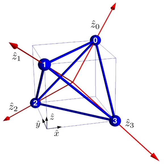
Figure 3: Sublattices of an up tetrahedron: 0,1,2,3 denote the four sublattices and $\hat{z}_{0}$, $\hat{z}_{1}$, $\hat{z}_{2}$, $\hat{z}_{3}$ represent the four respective local quantization axes (see Eq. LABEL:eq_local_basis in Appendix LABEL:appendix_spin_axis).

A central feature of the doublets in Eq. 2 is that under time reversal ($\mathcal{T}$) they transform as $\mid\pm\rangle\rightarrow\mid\mp\rangle$ such that the pseudo-spins transform as shown in Eq. 1.

II.1 The spin exchange physics of non-Kramers quantum spin ice

The pseudo-spins at different sites interact via regular spin exchanges and the minimal symmetry allowed spin Hamiltonian for non-Kramers spin ice is given by [rau, PhysRevB.83.094411, PhysRevLett.105.047201]

$$H_{0}=\sum_{\langle ij\rangle} \left[J_{zz}s_{i}^{z}s_{j}^{z}-J_{\pm}(s_{i}^{+}s_{j}^{-}+s_{i}^{-}s_{j}^{+})\right]+\cdots$$ (3)

where $\cdots$ denote other symmetry allowed terms (including further neighbour ones) which do not immediately destabilise the QSL. In fact, their main effect in the QSL phase is to renormalise the dispersion of the excitations of the quantum spin ice [sungbin2012, PhysRevB.90.214430]. We neglect them here and their effects can be taken into account systematically along the lines discussed in the rest of this work.

Experiments reveal the exchange coupling to be strongly anisotropic ($J_{zz}\gg J_{\pm}$). Also, $J_{zz}\approx 1.6K$, [kimura] which is two orders of magnitude smaller than the single ion crystal field gap. This justifies the use of single ion crystal field states to treat the problem perturbatively.

Interestingly, the transformation of the non-Kramers doublet under $\mathcal{T}$ in Eq. 1 leads to an unusual Zeeman coupling in such materials. The external magnetic field, being odd under time reversal, can couple linearly only with $s^{z}$ but not with $s^{x}$ and $s^{y}$. The latter, however, can couple to the magnetic field quadratically. The complete onsite Zeeman Hamiltonian can be found in Ref. [adarsh].

III Linear Magnetoelastic coupling in non-Kramers systems

Having discussed the spin physics, we now turn to the linear magnetoelastic coupling in non-Kramers systems. From the point of view of symmetry analysis, the structure of such a linear coupling is quite straightforward. For a single tetrahedron, the linear coupling can be obtained starting with the eight-dimensional vector space spanned by the time reversal even transverse components, $(s_{i}^{x},s_{i}^{y})$, of the spins on four corners of a tetrahedron (Fig. 3). This is then decomposed into the irreducible representations of the tetrahedral group, $T_{d}$, as

$$\mathbf{e}\oplus\mathbf{t}_{1}\oplus\mathbf{t}_{2}$$ (4)

where $\mathbf{e}$ denotes the doublet and $\mathbf{t_{1}}$, $\mathbf{t_{2}}$ represent two triplets with different symmetry transformations (see Table LABEL:table_spin_transformation in Appendix LABEL:appendix_symmetry_of_spins). Similarly, the (optical) normal vibrational modes of bond distortions of a tetrahedron are decomposed as,

$$\mathbf{a}_{1}\oplus\mathbf{e}\oplus\mathbf{t}_{2}$$ (5)

where $\mathbf{a}_{1}$ is the singlet. It is evident from the above decomposition that $\mathbf{e}$ and $\mathbf{t}_{2}$ vibrational (optical) modes of a tetrahedron can linearly couple to the transverse components of the non-Kramers doublet. Since the complete symmetry of the pyrochlore is $T_{d}\times\mathcal{I}$ (with $\mathcal{I}$ being the inversion), the complete representation is obtained by taking symmetric and antisymmetric combinations of the previous representations to form the ’g’ and ’u’ modes, which are even and odd under spatial inversion respectively.

As Raman scattering is insensitive to inversion-odd modes, we only consider the $\mathbf{e_{g}}$ and $\mathbf{t_{2g}}$ modes. Hence, the symmetry allowed magnetoelastic coupling for the Raman active modes is given by

$$H^{(e)}_{sp}=\sum_{\mathbf{r},p=1,2}J^{(e)}_{sp}\zeta^{(e)}_{p,g}(\mathbf{r})\left(Q^{(e)}_{p}(\mathbf{r},A)+Q_{p}^{(e)}(\mathbf{r},B)\right)$$ (6)

for the $\mathbf{e_{g}}$ modes and

$$H^{(t_{2})}_{sp}=\sum_{\mathbf{r},p=1,2,3}J^{(t_{2})}_{sp}\zeta^{(t_{2})}_{p,g}(\mathbf{r})\left(Q_{p}^{(t_{2})}(\mathbf{r},A)+Q_{p}^{(t_{2})}(\mathbf{r},B)\right)$$ (7)

for the $\mathbf{t_{2g}}$ modes. Here $\mathbf{r}$ denotes the centre of an up tetrahedron and $A/B$ denotes the two sublattices of the underlying diamond lattice, dual to the pyrochlore. $Q^{(e)}_{p}(\mathbf{r},A/B)$ and $Q^{(t_{2})}_{p}(\mathbf{r},A/B)$ respectively span the $\mathbf{e}$ and $\mathbf{t_{2}}$ irreducible sector for the spins. For a single up tetrahedron (Fig. 3), they are given by

$$Q^{(e)}_{1}=s^{x}_{0}+s^{x}_{1}+s^{x}_{2}+s^{x}_{3}$$

$$Q^{(e)}_{2}=s^{y}_{0}+s^{y}_{1}+s^{y}_{2}+s^{y}_{3}$$ (8)

and

$$Q^{(t_{2})}_{1} =\frac{1}{2}(-s^{x}_{0}+s^{x}_{1}+s^{x}_{2}-s^{x}_{3})$$

$$Q^{(t_{2})}_{2} =\frac{1}{4}(-s^{x}_{0}-s^{x}_{1}+s^{x}_{2}+s^{x}_{3})+\frac{\sqrt{3}}{4}(s^{y}_{0}+s^{y}_{1}-s^{y}_{2}-s^{y}_{3})$$

$$Q^{(t_{2})}_{3} =\frac{1}{4}(s^{x}_{0}-s^{x}_{1}+s^{x}_{2}-s^{x}_{3})+\frac{\sqrt{3}}{4}(s^{y}_{0}-s^{y}_{1}+s^{y}_{2}-s^{y}_{3})$$ (9)

Finally, $\zeta^{(e)}_{p,g}(\mathbf{r})$ and $\zeta^{(t_{2})}_{p,g}(\mathbf{r})$ are the ${\bf e_{g}}$ and $\mathbf{t_{2g}}$ normal modes of pyrochlore lattice. These normal modes are given by, $\zeta_{p,g}^{(\rho)}(\mathbf{k})=b^{(\rho)}_{p,\mathbf{k}}+b^{(\rho)\dagger}_{p,\mathbf{-k}}$ where $b^{(\rho)\dagger}_{p,\mathbf{k}}$ is the creation operator of the phonons of the $\rho$ irreducible representation, with the bare phonon Hamiltonian given by

$$H_{\zeta}=\sum_{\rho}\sum_{\mathbf{k},p}\omega^{(\rho)}_{\mathbf{k}}\left(b^{(\rho)\dagger}_{p,\mathbf{k}}b^{(\rho)}_{p,\mathbf{k}}+\frac{1}{2}\right).$$ (10)

An alternate and somewhat more microscopic derivation of the above physics can be obtained by considering the coupling of the doublet wave functions of Eq. 2 with the phonons, which also gives rise to phonon mediated coupling between different crystal field states. The physics of such couplings will be discussed elsewhere [j32].

The above linear coupling makes the non-Kramers spin ice materials susceptible to spin Jahn-Teller distortions, where the spin entropy can be quenched by distorting the lattice and thereby splitting the doublet. Indeed, in some samples of Pr${}_{2}$Zr${}_{2}$O${}_{7}$, signatures of such splitting have been observed [wen-disorder, matsuhira2009spin], accompanied with random lattice distortions. However, more recent higher quality samples appear devoid of such distortions, suggesting controlled suppression of Jahn-Teller distortions in better quality single crystals [Comsatoru].

In the absence of static deformation of the crystal field environment, the above linear spin-phonon coupling helps to enhance the transverse fluctuations in the spin ice manifold, which could stabilise a U(1) QSL phase via magneto-distortive dynamics [Comsatoru].

To study the effect of linear magnetoelastic coupling (Eq. 6 and Eq. 7) via the Raman experiments on quantum spin ice, we need to re-write the above spin-phonon coupling in terms of the coupling of the phonon to the low-energy excitations of the U(1) QSL. To derive this, for completeness we briefly review the well-known mapping between the spins and low-energy gauge theory for quantum spin ice  [savary, hermele, doron, sungbin2012] next.

IV quantum spin ice

The description of the quantum spin ice is obtained starting with a magnetic monopole charge density operators [savary, sungbin2012, PhysRevLett.95.217201] $\mathcal{Q}_{\mathbf{r}}$, defined at the centre of a tetrahedron at $\mathbf{r}$, as

$$\mathcal{Q}_{\mathbf{r}}=\eta_{\mathbf{r}}\sum_{\mu}s^{z}_{\mathbf{r},\mathbf{r}+\eta_{\mathbf{r}}\mathbf{e}_{\bm{\mu}}}$$ (11)

where, $\eta_{\mathbf{r}}=1~{}(-1)$ for $\mathbf{r}\in$ up (down) tetrahedra of the pyrochlore lattice and $\mathbf{e}_{\bm{\mu}}$ is the vector connecting centres of the two nearest neighbour tetrahedra directed from up to down (see Appendix LABEL:appendix_lattice_vectors). We call the positively charged particles monopoles and negatively charged ones antimonopoles. The creation (annihilation) operators for the monopoles are defined as $\phi_{\mathbf{r}}^{\dagger}$ ($\phi_{\mathbf{r}}$) such that it satisfies, $[\mathcal{Q}_{\mathbf{r}},\phi^{\dagger}_{\mathbf{r^{\prime}}}]=\delta_{\mathbf{r,r^{\prime}}}\phi^{\dagger}_{\mathbf{r}}$.

The relation between the monopole and spin operators is given by

$$s^{+}_{\mathbf{r},\mathbf{r}+\mathbf{e}_{\bm{\mu}}}=\frac{1}{2}\phi^{\dagger}_{\mathbf{r}}~{}e^{iA_{\mathbf{r},\bm{\mu}}}\phi_{\mathbf{r}+\mathbf{e}_{\bm{\mu}}}$$ (12)

where $\mathbf{r}\in$ up tetrahedron and $A_{\mathbf{r},\bm{\mu}}$ represents the compact $U(1)$ dual gauge field on the bond joining $\mathbf{r}$ and $\mathbf{r}+\mathbf{e}_{\bm{\mu}}$ (In other words, they live on the links of the dual diamond lattice). The spin operators remain invariant under the following $U(1)$ gauge transformation.

$$\phi_{\mathbf{r}}\rightarrow\phi_{\mathbf{r}}e^{-i\theta_{\mathbf{r}}},\indent\indent A_{\mathbf{r},\bm{\mu}}\rightarrow A_{\mathbf{r},\bm{\mu}}+(\theta_{\mathbf{r}+\mathbf{e}_{\bm{\mu}}}-\theta_{\mathbf{r}})$$ (13)

The compactness of the gauge field allows for dual electric charge excitations [hermele] which are gapped in the QSL.

Using the above mapping the spin Hamiltonian (Eq. 3) can be written in terms of the gauge fields, monopoles, and the charges to obtain the lattice gauge theory description of quantum spin ice. This is given by Eq. LABEL:eq_bare_monopole_hamiltonian in Appendix LABEL:appen_lgt along with other relevant details.

IV.1 The gapless emergent photons

In the limit $J_{zz}\gg J_{\pm}$, the magnetic monopoles have a gap of $\mathcal{O}(J_{zz})$ and can be integrated out. The low-energy Hamiltonian is obtained in terms of the fluctuations of the dual $U(1)$ gauge field $A_{\mathbf{{r},\bm{\mu}}}$. This leads to the well-known ring-exchange Hamiltonian that can be obtained either via degenerate perturbation theory of Eq. 3 [hermele] or equivalently integrating out the magnetic monopoles from Eq. LABEL:eq_bare_monopole_hamiltonian. This is given by

$$H_{eff}=\frac{U}{2}\sum_{\mathbf{r},\mu}B_{\mathbf{r},\bm{\mu}}^{2}-\frac{K}{2}\sum_{\hexagon}\cos\left(\sum_{\mathbf{r},\mu\in\hexagon}A_{\mathbf{r},\bm{\mu}}\right)$$ (14)

where $B_{\mathbf{r},\bm{\mu}}$($=s^{z}_{\mathbf{r},\mathbf{r}+\mathbf{e}_{\bm{\mu}}}$, $\mathbf{r}\in$ up tetrahedron) is the emergent magnetic field that is canonically conjugate to the dual vector potential, i.e., $\left[A_{\mathbf{r},\bm{\mu}},B_{\mathbf{r^{\prime}},\bm{\nu}}\right]=i\delta_{\mathbf{r,r^{\prime}}}\delta_{\mu,\nu}$, $U$ is a Lagrange multiplier imposing the half-integer constraint on magnetic fields, and $K\sim\frac{J_{\pm}^{3}}{J_{zz}^{2}}$. The emergent electric field is given by ${\bf E}_{\hexagon}=\sum_{\mathbf{r},\mu\in\hexagon}A_{\mathbf{r},\mu}$ where $\sum_{\mathbf{r},\mu\in\hexagon}$ denotes the lattice curl around the hexagonal loops of the pyrochlore.

The QSL corresponds to the deconfined phase ($\mid K\mid\gg U$) of the above Hamiltonian. In this limit, the energy for the pure gauge theory can be minimized by setting up zero ($\pi$) electric flux through all the elementary hexagonal plaquettes for $K>0$ ($K<0$) [sungbin2012]. These we shall term as $0$ and $\pi$-flux phases, respectively, since the magnetic monopoles hopping on the diamond lattice (see below) see this electric flux.

The low-energy excitations of the gauge theory can then be captured by expanding the cosine term up to quadratic order about these static electric flux configurations. This gives rise to a free Maxwell theory with two transverse polarised gapless photon excitations and their dispersion is given by [rau2017],

$$\varepsilon_{\mathbf{k}}=c_{e}\mid\mathbf{k}\mid$$ (15)

where $c_{e}=\sqrt{UK}$ is the speed of emergent light.

IV.2 The gapped magnetic monopole

The dynamics of the bare magnetic monopoles, on the other hand can be obtained in a GMFT approximation of Eq. LABEL:eq_bare_monopole_hamiltonian by freezing the gauge fluctuation [savary] (see Appendix LABEL:appen_lgt for details).

For $K>0$, the ground state of the pure gauge theory is in the zero electric flux sector (see above) where the gauge mean field ansatz can be chosen as $A_{\mathbf{r},\bm{\mu}}=0$. The bare band structure for the two flavours ($A$ and $B$) of magnetic monopoles is then given by [savary]

$$\epsilon^{0}_{\mathbf{k}}=\sqrt{2J_{zz}\left(\lambda-\frac{J_{\pm}}{2}\sum_{\mu>\nu}\cos\left(\mathbf{k}\cdot(\mathbf{d_{\mu}-d_{\nu}})\right)\right)}$$ (16)

where $\lambda$ is a Lagrange multiplier introduced to take into account the unitary constraint of the monopole operators (see Appendix LABEL:appen_zero_mon_band) at the mean-field level.

For $K<0$ on the other hand, the monopoles hop in a $\pi$-flux background per hexagonal plaquette. This can be implemented by choosing a suitable gauge [sungbin2012] (also see Fig. LABEL:fig_unit_pi in Appendix LABEL:appen_lgt) which doubles the size of magnetic unit cell, leading to four flavours of monopoles. The details of their band structure is summarized in Appendix LABEL:appendix_pi_flux_1. In contrast to the zero flux phase, two non-degenerate bands (denoted as $\epsilon^{\pi}_{+}({\bf k})$ and $\epsilon^{\pi}_{-}({\bf k})$) appear due to the presence of non-trivial background flux. It will be shown in Sec. VII.2 that this leads to a very different Raman response of these two QSL phases.

The bare band structure of monopoles gets further renormalised due to the gauge fluctuations [PhysRevLett.127.117205]. However, in the following discussion, we will assume the monopole-gauge coupling constant to be small, so that these only lead to a sub-leading corrections of the GMFT results (see Sec. VII.3). We shall comment on the merits/shortcomings of this approximation in the summary.

IV.3 The gapped electric charge

The electric charges or the point defects of the gauge field appear due to the $2\pi$ ambiguity of defining the compact vector potential [hermele, doron]. The fluctuations of the electric field are not small near these excitations and the expansion of the cosine term (see Sec. IV.1) is not possible. Unlike the magnetic monopoles and the photons, these excitations are non-local in terms of the underlying spins and their properties are better captured in the dual description [hermele, doron, motrunich, gang2016] of the emergent gauge theory describing the bosonic electric charges, $\Psi_{\bf\mathsf{r}}$, hopping on the dual diamond lattice, ${\bf\mathsf{r}}$, via [doron, gang2016]

$$H_{charge}=-\sum_{\langle{\bf\mathsf{r,r^{\prime}}}\rangle}t~{}e^{-i2\pi{\bf a_{\mathsf{r,r^{\prime}}}}}\Psi^{\dagger}_{\bf\mathsf{r}}\Psi_{\bf\mathsf{r^{\prime}}}+m\sum_{\mathsf{r}}\Psi^{\dagger}_{\bf\mathsf{r}}\Psi_{\bf\mathsf{r}}$$ (17)

where ${\bf a_{\mathsf{r,r^{\prime}}}}$ is the vector potential dual to $A_{\mathbf{r},\bm{\mu}}$; $t$ is the effective hopping strength and $m$ is the chemical potential for the electric charges. The vector potential admits only integer values and is defined by,

$$\left(\nabla\times{\bf a_{\mathsf{r,r^{\prime}}}}\right)_{\hexagon^{*}}=\sum_{{\bf\mathsf{rr^{\prime}}}\in\hexagon^{*}}{\bf a_{\mathsf{r,r^{\prime}}}}=B_{\mathbf{r},\bm{\mu}}-B^{0}_{\mathbf{r},\bm{\mu}}$$

$\hexagon^{*}$ denotes the dual elementary hexagonal plaquettes and $B^{0}_{\mathbf{r},\mu}$ is a static divergenceless background field. Since there is a single spin-$1/2$ on every pyrochlore site, the gauge field has a background $\pi$-flux in every dual hexagonal plaquette [gang2016] such that in the gauge mean-field limit (where we ignore the fluctuations of ${\bf a_{\mathsf{r,r^{\prime}}}}$ around the background), the dynamics of electric charges reduces to the problem of bosons hopping on the diamond lattice subject to the background $\pi$-flux in every hexagonal plaquette. This can be solved using a proper gauge choice and gives rise to 12 soft modes [gang2016, doron]. We denote the soft modes as $\psi_{i}(i=1,...,12)$. As mentioned earlier (see Sec. I), the energy gap of the electric charges, $\Delta_{c}$, in the QSL phase is $\sim\mid J_{\pm}\mid^{3}/J^{2}_{zz}$. Within the hopping model, Eq. 17, minimum gap of the electric charges is $\Delta_{c}=m-2\sqrt{2}t$.

The band structure of the electric charges gets further renormalised due to the gauge fluctuations. Compared to magnetic monopoles, they have a much smaller energy gap, and hence on general grounds, their coupling with the emergent photon is expected to be relatively much stronger. However, in order to keep our analysis tractable, we neglect such effects within our GMFT approach and only take them into account perturbatively.

V Magnetoelastic coupling in non-Kramers quantum spin ice

The effect of the magnetoelastic coupling in the QSL phase can be analyzed by studying the coupling of the phonon to the emergent excitations using the mapping from spins to gauge charges discussed above. For the linear coupling in Eqs. 6 and 7, the resultant interactions are given below.

V.1 The magnetic monopole-phonon coupling

Here we obtain the direct coupling between the phonon and the magnetic monopole. From Eq. 6, we get, for the $\mathbf{e_{g}}$ phonons :

$$H^{(e)}_{sp}=\frac{J^{(e)}_{sp}}{2}\sum_{\mathbf{r}}\sum_{\mu=0}^{3}\zeta_{-,g}^{(e)}({\mathbf{r}})\left[\phi_{{\mathbf{r}},A}^{\dagger}e^{iA_{\mathbf{r},\bm{\mu}}}\phi_{{\bf r+d_{\bm{\mu}}},B}\right.~{}~{}~{}~{}~{}~{}$$

$$\left.+\phi_{{\bf r-d_{\bm{\mu}}},A}^{\dagger}e^{iA_{{\bf r-d_{\bm{\mu}},\bm{\mu}}}}\phi_{{\bf r},B}\right]+h.c.$$ (18)

where,

$$\zeta^{(e)}_{\pm,g}({\bf r})=\zeta^{(e)}_{1,g}({\bf r})\pm i\zeta^{(e)}_{2,g}({\bf r})$$

are the displacement fields and from Eq. 7 for the $\mathbf{t_{2g}}$ phonons,

$$H^{(t_{2})}_{sp}=$$

$$\frac{J^{(t_{2})}_{sp}}{2}\sum_{\bf r}\sum_{\mu=0}^{3}\sum_{p=1}^{3}\left(\zeta^{(t_{2})}_{p,g}({\bf r})L^{(t_{2})}_{p,x,\mu}-i\zeta^{(t_{2})}_{p,g}({\bf r})L^{(t_{2})}_{p,y,\mu}\right)$$

$$\times\left[\phi^{\dagger}_{{\mathbf{r}},A}e^{iA_{\mathbf{r},\bm{\mu}}}\phi_{{\bf r+d_{\mu}},B}+\phi^{\dagger}_{{\mathbf{r}-\mathbf{d}_{\bm{\mu}}},A}e^{iA_{{\mathbf{r}-\mathbf{d}_{\bm{\mu}}},{\bm{\mu}}}}\phi_{{\bf r},B}\right]+h.c.$$ (19)

The form factors $L^{(t_{2})}_{p,\alpha,\mu}$ are obtained via the relation $Q^{(t_{2})}_{p}=\sum_{\alpha=x,y}~{}\sum_{\mu=0}^{3}L^{(t_{2})}_{p,\alpha,\mu}s^{\alpha}_{\mu}$, their explicit forms can then follow from Eq. 9.

Both these interactions give rise to a Yukawa type coupling between the phonons and the monopole bilinear of the form $\zeta\phi^{\dagger}e^{iA}\phi$, albeit with different form factors. The corresponding bare vertex is shown in Fig. 2(a). It is clear from the interaction that the above coupling allows for a phonon to decay into a monopole-antimonopole pair: new low-energy scattering channels for the phonons inside the QSL phase open up. Note that while the bare monopole hopping preserves the sub-lattice flavour of the monopole, the above vertex mixes them, keeping only the total monopole number preserved.

Figure 4: GMFT Feynman diagram for phonon and magnetic monopole interaction (described by Eqs. 20 and 21) in the zero flux phase: (see Fig. 2(a) for further details).

Within GMFT, we assume that the gauge fluctuations are weak and can be taken into account perturbatively. Thus, within GMFT, the bare vertex for the magnetic monopole-phonon interaction is given by Fig. 4, where the gauge fluctuations have been neglected. Indeed, we shall show that within a perturbative treatment of the gauge field, the temperature dependence of the corrections due to gauge fluctuations are sub-leading compared to the mean-field results at low temperatures (see Sec. VII.3). In momentum space, GMFT vertices are given by

$$H^{(e)}_{sp}=\frac{J^{(e)}_{sp}}{2\sqrt{N}}\sum_{\mathbf{k},\mathbf{k^{\prime}}}\left[(\alpha^{(e)}_{\mathbf{k}}+\alpha^{(e)}_{\mathbf{k^{\prime}}})\zeta^{(e)}_{-,g}(\mathbf{k}-\mathbf{k^{\prime}})\phi^{\dagger}_{\mathbf{k},A}\phi_{\mathbf{k^{\prime}},B}\right.$$

$$\hskip 199.16928pt+h.c.\Big{]}$$ (20)

$$H_{sp}^{(t_{2})}=\frac{J_{sp}^{(t_{2})}}{2\sqrt{N}}\sum_{\mathbf{k},\mathbf{k^{\prime}}}\sum_{p=1}^{3}\Big{[}(\alpha^{(t_{2})}_{p,\mathbf{k}}+\alpha^{(t_{2})}_{p,\mathbf{k^{\prime}}})\times$$

$$~{}~{}~{}~{}~{}~{}~{}~{}~{}~{}~{}~{}~{}~{}~{}~{}~{}~{}~{}~{}~{}~{}~{}~{}~{}~{}\times\zeta^{(t_{2})}_{p,g}(\mathbf{k}-\mathbf{k^{\prime}})\phi_{\mathbf{k},A}^{\dagger}\phi_{\mathbf{k^{\prime}},B}+h.c.\Big{]}$$ (21)

where $N$ is the total number of unit cells, while $\alpha^{(e)}_{\bf k}$ and $\alpha^{(t_{2})}_{p,{\bf k}}$s are vertex functions of the ${\bf e_{g}}$ and ${\bf t_{2g}}$ coupling, respectively, whose forms are given in Appendix LABEL:appendix_zero_flux_vertex.

V.2 The (emergent) photon-phonon coupling

To obtain the coupling between phonon and emergent photon, once again we integrate out the gapped magnetic monopoles (as in Sec. IV.1) in presence of the magnetoelastic coupling described by Eq. 18 and 19. The leading coupling between phonon and gauge field is obtained in fourth-order of the perturbation theory [etienne]. For the $\mathbf{e_{g}}$ phonons, this gives rise to

$$H_{phonon-photon}=-\frac{J_{sp}^{(e)2}J_{\pm}^{2}}{2J_{zz}^{3}}\sum_{\hexagon}\left(\sum_{{\bf r}\in\hexagon}\bm{\zeta}^{(e)}_{g}({\bf r})\cdot\bm{\zeta}^{(e)}_{g}({\bf r})\right)$$

$$\times\cos\left[{\bf E}_{\hexagon}\right]$$ (22)

In the deconfined QSL phase, the cosine term in the Hamiltonian above can be expanded up to quadratic order as $\cos{\bf E}\approx 1-{\bf E}^{2}/2$. At low energies, the constant term in the expansion leads to a quadratic term in the phonon. This renormalises the frequency of the phonon by a constant shift without affecting its linewidth.

The leading order coupling between the phonon and the emergent photon, in the continuum limit is given by

$$\mathcal{H}_{phonon-photon}=J_{ph-ph}\int d^{3}{\bf r}~{}\bm{\zeta}^{(e)}_{g}({\bf r})\cdot\bm{\zeta}^{(e)}_{g}({\bf r})~{}{\bf E}^{2}({\bf r})$$ (23)

where $J_{ph-ph}\sim\frac{J_{sp}^{(e)2}J_{\pm}^{2}}{4J_{zz}^{2}l^{3}}$ with $l$ being the lattice length-scale. As expected, the phonons cannot simply couple to the dual gauge field since they do not carry the emergent gauge charge. Instead, they couple to the gauge invariant electric field. Further, since the Raman active phonons are even under inversion, they can only couple to the electric field at quadratic order. We note, in passing, that the antisymmetric phonon modes (’u’ modes) on the other hand are allowed to couple linearly to the emergent electric field. Such interaction effects can be probed using infrared spectroscopy [etienne].

In momentum space, Eq. 23 takes the form

$$\mathcal{H}_{phonon-photon}=\int \prod_{i=1}^{4}~{}d^{3}{\bf k}_{i}~{}\mathcal{G}^{\alpha\beta}({\bf k_{1},k_{2},k_{3},k_{4}})$$

$$\times\left(\bm{\zeta}^{(e)}_{g}({\bf k_{1}})\cdot\bm{\zeta}^{(e)}_{g}({\bf k_{2}})\right)~{}A^{\alpha}_{\bf k_{3}}A^{\beta}_{\bf k_{4}}$$ (24)

where the interaction vertex is given by

$$\mathcal{G}^{\alpha\beta}({\bf k_{1},k_{2},k_{3},k_{4}})=\frac{J_{ph-ph}}{N}~{}\left[-{\bf k_{3}\cdot k_{4}}\delta_{\alpha\beta}+k_{3}^{\beta}k_{4}^{\alpha}\right]$$

$$\times\delta({\bf k_{1}+k_{2}+k_{3}+k_{4}})$$ (25)

The above interaction is shown in Fig. 2(b), where the circle represents the gauge invariant dipolar vertex function, $\mathcal{G}^{\alpha\beta}$. Such decay processes for phonons in a QSL phase give rise to an additional contribution to the phonon linewidth similar to that due to the monopoles, albeit at a different energy-scale.

V.3 The electric charge-phonon coupling

Similar to the phonon-magnetic monopole coupling, the phonons also interact with the electric charges via a Yukawa coupling as shown in Fig. 2(c) (again, the electric charge creation/annihilation operators are not gauge invariant and hence cannot couple to the phonons linearly).

To derive the coupling between the phonons and the electric charges, we construct the bilinears of the soft electric charge modes with appropriate symmetry that can couple to a particular polarisation of the phonon. Here we analyze only the $\mathbf{e_{g}}$ couplings and the interaction is given by,

$$H_{phonon-charge}=J^{(e)}_{ph-ch}\sum_{\bf r} \left(\zeta^{(e)}_{1,g}({\bf r})\Theta_{1}({\bf\mathsf{r}})\right.$$

$$~{}~{}~{}\left.+\zeta^{(e)}_{2,g}({\bf r})\Theta_{2}({\bf\mathsf{r}})\right)$$ (26)

where $(\Theta_{1},\Theta_{2})$ forms an $\mathbf{e_{g}}$ doublet and is given by,

$$\Theta_{1}=\psi_{1}^{*}\psi_{1}+\psi_{11}^{*}\psi_{11}-\psi_{3}^{*}\psi_{3}-\psi_{9}^{*}\psi_{9}$$

$$\Theta_{2}=-\psi_{1}^{*}\psi_{1}-\psi_{11}^{*}\psi_{11}-\psi_{3}^{*}\psi_{3}-\psi_{9}^{*}\psi_{9}+2(\psi_{5}^{*}\psi_{5}+\psi_{7}^{*}\psi_{7})$$ (27)

where $\psi_{i}$ ($i=1,2,\cdots 12$) are the soft modes of the electric charges as obtained in Ref. [gang2016] and discussed in the previous section. The above interaction is shown in Fig. 5.

Figure 5: GMFT Feynman diagram for phonon and electric charge interaction (described by Eq. 26): (see Fig. 2(c) for further details).

Due to the above magnetoelastic coupling, phonons acquire a finite lifetime by scattering with the excitations of the QSL. In the next three sections (Sec. VII, VIII and IX), we compute the lifetime of the phonons and their typical low-temperature behaviour in order to probe the non-Kramers U(1) QSLs.

VI Raman Scattering of the phonons in quantum spin ice phase

The Raman vertex for the phonon is given by [porto]

$$H_{Raman} =\int\mathbf{P}(\mathbf{r})\cdot\mathbf{E}_{ext}(\mathbf{r})~{}d^{3}\mathbf{r}$$ (28)

where ${\bf P}({\bf r})$ is the electric dipole moment and ${\bf E}_{ext}({\bf r})$ is the external electric field (to be distinguished from the emergent electromagnetism). Relegating details to Appendix LABEL:appen_phononraman, we find the Raman scattering cross-section [devereaux],

$$\frac{d^{2}\sigma(\mathbf{q},\omega)}{d\Omega d\omega_{s}}\propto R(\mathbf{q},\omega),$$ (29)

where for a thermal system, by Fermi’s Golden rule,

$$R(\mathbf{q},\omega)=\sum_{i,f}\frac{e^{-\beta E_{i}}}{Z}\mid\langle f\mid H_{Raman}\mid i\rangle\mid^{2}\delta(E_{f}-E_{i}-\omega)$$ (30)

Here $\mathbf{q}=\mathbf{q_{in}-q_{out}}$ is the net momentum transferred to the system by the Raman process and $\omega$ is the difference between the frequency of incident and scattered photons. As the speed of light is very large compared to that of the phonons, only the $\mathbf{q}\rightarrow 0$ regime of the Brillouin zone can be probed by Raman scattering. Further, $\mid i\rangle$, $\mid f\rangle$ denote the initial and final state of the phonons respectively, with energies $E_{i}$ and $E_{f}$. Finally, $Z$ is the partition function for a Gibbs distribution at temperature, $T=1/\beta$.

At low temperatures, the initial state can be approximated by the ground state. Also, we can see from the Raman vertex (Eqs. 28 and LABEL:eq_ramver_appen) that the scattering matrix element is non-zero only when $\mid i\rangle$ and $\mid f\rangle$ differ by a single phonon, as higher phonon processes are suppressed at low temperatures. So at low temperatures, $\mid f\rangle$ should be chosen from the single phonon sector leading to

$$R(\mathbf{q},\omega)\propto-\frac{\pi n(\omega)e^{\beta\omega}}{Z}e^{-\beta E_{0}}\lim_{\delta\rightarrow 0^{+}}\mathcal{I}m[G_{\zeta}(\mathbf{q},\omega+i\delta)]$$ (31)

where, $n(\omega)=\frac{1}{e^{\beta\omega}-1}$ is the Bose-factor and $G_{\zeta}(\mathbf{q},\omega+i\delta)$ is the retarded Green’s function of the phonon. This can be calculated from the analytic continuation of the Matsubara Green’s function, $G_{\zeta}({\bf q},i\omega)$, given by

$$G_{\zeta}(\mathbf{q},i\omega) =-\int_{0}^{\beta}d\tau\langle\hat{\mathcal{T}}\left(\zeta({\bf q},\tau)\zeta(-{\bf q},0)\right)\rangle e^{i\omega\tau}$$

$$=-\frac{2\omega_{\mathbf{q}}}{\omega^{2}+\omega_{\mathbf{q}}^{2}+2\omega_{\mathbf{q}}\Sigma_{\zeta}({\bf q},i\omega)}$$ (32)

where $\omega_{\bf q}$ is the bare dispersion of the phonon (obtained from Eq. 10) and $\Sigma_{\zeta}({\bf q},i\omega)$ is its self-energy arising from the interaction with the QSL excitations. Here, for simplicity of the expression, we have suppressed the superscript denoting the irrep of the phonon. Eq. 31 results in a Lorentzian lineshape. The position of the peak of this curve is shifted from the non-interacting one by

$$|\Delta_{Raman}|=\mathcal{R}e\left[\Sigma_{\zeta}({\bf q},\omega+i\delta)\right]$$ (33)

and the full-width at half maximum of the Lorentzian is given by

$$\Gamma=2\mid\mathcal{I}m\left[\Sigma_{\zeta}({\bf q},\omega+i\delta)\right]\mid$$ (34)

which can then be directly compared with experiment.

We now focus on understanding the frequency and temperature dependence of the linewidth, $\Gamma$, in detail, in order to extract the information it contains about the QSL excitations via the linear magnetoelastic coupling. The real part can be computed from the imaginary part using the standard Kramers-Kronig theorem [mahan]. Since the three QSL excitations are separated in energy scales, we expect that they dominate the linewidth in different frequency windows. Therefore, we particularly focus on the frequency dependence of the linewidth.

VII Self-energy of the phonon due to phonon-magnetic monopole coupling

We now calculate the self-energy of the phonons and hence the broadening of the phonon peaks due to the phonon-monopole interaction. We calculate the effect of the coupling in a perturbative approach both in the zero and $\pi$-flux phases.

VII.1 Zero flux phase

The first non-zero contribution to the self-energy comes at second order, $\mathcal{O}(J_{sp}^{(\rho)2})$, by computing the bubble diagram of Fig. 6. Within GMFT, for the zero flux phase, the self-energy is given by,

Figure 6: Self-energy of the phonon due to the phonon-magnetic monopole interaction (see Fig. 4)

$$\Sigma^{0}_{\zeta^{(\rho)}}(\mathbf{q},i\Omega)= -\frac{J^{(\rho)2}_{sp}}{4N\beta}\sum_{\mathbf{k},\omega}\mid\alpha^{(\rho)}_{\mathbf{k}}+\alpha^{(\rho)}_{\mathbf{k+q}}\mid^{2}$$

$$\times G^{0}_{\phi}(\mathbf{k},A,i\omega)G^{0}_{\phi}(\mathbf{k+q},B,i(\omega+\Omega))$$ (35)

where the time ordered Green’s function ($G_{\phi}^{0}$) for monopoles in the zero flux phase is defined as (see Eq. LABEL:eq_mon_action_zero in Appendix LABEL:appen_zero_mon_band),

$$G^{0}_{\phi}(\mathbf{k},A/B,i\omega) =\int_{0}^{\beta}d\tau\langle\hat{\mathcal{T}}\left(\phi_{\mathbf{k},A/B}(\tau)\phi^{\dagger}_{\mathbf{k},A/B}(0)\right)\rangle e^{i\omega\tau}$$

$$=\frac{2J_{zz}}{\omega^{2}+\left(\epsilon^{0}_{\mathbf{k}}\right)^{2}}$$ (36)

To obtain the broadening of the Raman peaks, we calculate the imaginary part of $\Sigma^{0}_{\zeta^{(\rho)}}(\mathbf{q},i\Omega\rightarrow\Omega+i\delta)$. Performing the frequency summation using standard Matsubara summation techniques [mahan], we get

$$\lim_{\delta\rightarrow 0}~{}\mathcal{I}m[\Sigma^{0}_{\zeta^{(\rho)}}(\mathbf{q},\Omega+i\delta)]=\frac{\pi J_{sp}^{(\rho)2}J_{zz}^{2}}{4N}\sum_{\mathbf{k}}\mid\alpha^{(\rho)}_{\mathbf{k}}+\alpha^{(\rho)}_{\mathbf{k+q}}\mid^{2}\left[\frac{n(\epsilon^{0}_{\mathbf{k}})-n(\epsilon^{0}_{\mathbf{k+q}})}{\epsilon^{0}_{\mathbf{k}}\epsilon^{0}_{\mathbf{k+q}}}\Big{(}\delta(\Omega+\epsilon^{0}_{\mathbf{{k+q}}}-\epsilon^{0}_{\mathbf{k}})-\delta(\Omega+\epsilon^{0}_{\mathbf{k}}-\epsilon^{0}_{\mathbf{k+q}})\Big{)}\right.$$

$$\left.+\frac{n(\epsilon^{0}_{\mathbf{k}})+n(\epsilon^{0}_{\mathbf{{k+q}}})+1}{\epsilon^{0}_{\mathbf{k}}\epsilon^{0}_{\mathbf{k+q}}}\Big{(}\delta(\Omega+\epsilon^{0}_{\mathbf{k}}+\epsilon^{0}_{\mathbf{k+q}})-\delta(\Omega-\epsilon^{0}_{\mathbf{k}}-\epsilon^{0}_{\mathbf{k+q}})\Big{)}\right]$$ (37)

where, $n(\epsilon^{0}_{\mathbf{k}})=\frac{1}{e^{\beta\epsilon^{0}_{\mathbf{k}}}-1}$ is the Bose occupation for the magnetic monopole with $\epsilon^{0}_{\mathbf{k}}$ being the single-particle dispersion within GMFT as given by Eq. 16.

The first two delta functions of Eq. 37 imply processes where a monopole scatters by absorption of a phonon (absorption process). The prefactor $(n(\epsilon^{0}_{\mathbf{k}})-n(\epsilon^{0}_{\mathbf{k+q}}))$ represents the net probability of such processes. On the other hand, the last two delta functions in Eq. 37 arise due to the conversion of a phonon into a monopole-antimonopole pair or vice-versa (pair production process, Fig. 1(c)). The prefactor $(1+n(\epsilon^{0}_{\mathbf{k}})+n(\epsilon^{0}_{\mathbf{k+q}}))$ represents the net probability of two competing processes- the first(second) is the annihilation (creation) of a phonon followed by creation (annihilation) of the monopole-antimonopole pair.

Eq. 37 is one of the central results of this work. It shows that the self-energy correction of the phonons arises from its coupling to the magnetic monopoles. We now analyze the self-energy, in particular, its frequency dependence, which can be detected in Raman scattering experiments. For Raman scattering, only the ${\bf q}\approx 0$ regime of the Brillouin zone is accessible. In this limit, clearly the probability of the absorption process of the phonons vanishes since the difference of the two Bose factors go to zero as ${\bf q}\rightarrow 0$, leading to

$$\Gamma(\Omega,T)=2\mid\mathcal{I}m[\Sigma^{0}_{\zeta^{(\rho)}}(\mathbf{q}=0,\Omega)]\mid=\frac{2\pi J_{sp}^{(\rho)2}J_{zz}^{2}}{N}\sum_{\mathbf{k}}\mid\alpha^{(\rho)}_{\mathbf{k}}\mid^{2}\Big{[}\frac{2n(\epsilon^{0}_{\mathbf{k}})+1}{(\epsilon^{0}_{\mathbf{k}})^{2}}\mid\Big{(}\delta(\Omega+2\epsilon^{0}_{\mathbf{k}})-\delta(\Omega-2\epsilon^{0}_{\mathbf{k}})\Big{)}\mid\Big{]}$$ (38)

From Eq. 16, we see that the bare monopole band structure is gapped with its minima at $\mathbf{k}=0$ and the energy gap, $\Delta_{0}=\sqrt{2J_{zz}\left(\lambda-3J_{\pm}\right)}$. It is evident from Eq. 38 that the splitting of phonons into a monopole-antimonopole pair occurs only if the phonon frequency is larger than the pair creation energy ($2\Delta_{0}$) such that $\Gamma\sim\Theta\left(\mid\Omega\mid-2\Delta_{0}\right)$. This is visible in Fig. 7, where we plot the linewidth, $\Gamma(\Omega,T)$ versus the frequency, $\Omega$, for various temperatures, $T$, for both the $\mathbf{e_{g}}$ and the $\mathbf{t_{2g}}$ modes, for $\Delta_{0}=1.26J_{zz}$ as an illustrative example for plotting. The profile of the curve remains qualitatively same as long as the constraint $\lambda>3J_{\pm}$ is satisfied, which defines the extent of the QSL. Apart from the dependence on the form factors, $\alpha_{\bf k}^{(\rho)}$, and the Bose factor, both these curves reflects the two-particle density of states profile of monopoles, shown in the inset of Fig. 7(b). The effect of the form factors can be noted from the qualitative difference of the two plots. Since $\alpha_{\mathbf{k}}^{(t_{2})}\rightarrow 0$ as $\mathbf{k}\rightarrow 0$ (from Eq. LABEL:eq_vertex_functions), the linewidth for $\mathbf{t_{2g}}$ smoothly vanishes for $\Omega\rightarrow 2\Delta_{0}$. By contrast, for $\mathbf{e_{g}}$, the vertex function ($\alpha_{\mathbf{k}}^{(e)}$) tends to a nonzero constant as $\mathbf{k}\rightarrow 0$ (from Eq. LABEL:eq_vertex_functions) and the linewidth shows a sharp behaviour even at zero momentum.

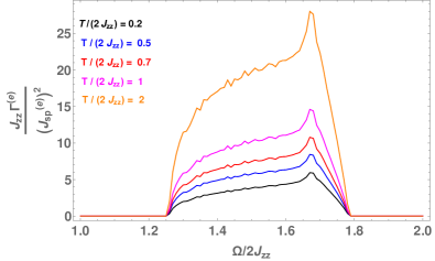
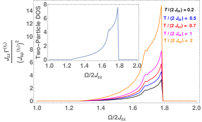
Figure 7: Frequency dependence of linewidth of (a) $\mathbf{e_{g}}$ and (b) $\mathbf{t_{2g}}$ phonons in the zero flux phase due to the phonon-magnetic monopole coupling: For both plots, we have chosen $\frac{\lambda}{2J_{zz}}=0.7$ and $\frac{J_{\pm}}{2J_{zz}}=0.1$ for illustrative purpose. The inset of (b) shows the two-particle density of states (DOS) of magnetic monopoles for the same values of $\lambda/2J_{zz}$ and $J_{\pm}/2J_{zz}$.

VII.2 $\pi-$ flux phase

The phonon-magnetic monopole coupling in the $\pi-$flux phase is obtained from the linear spin-phonon coupling of Eq. 6 and Eq. 7 via parton decomposition of the spins and freezing the gauge fluctuations to a suitable GMFT ansatz as described in Sec. IV.2. Focusing only on the $\mathbf{e_{g}}$ phonons, the phonon-monopole coupling is given by,

$$H^{(e)}_{sp}=\frac{J^{(e)}_{sp}}{2\sqrt{N}}\sum_{\mathbf{k}}\sum_{\mu,\nu=1,2}\left(M^{\mu\nu}_{\mathbf{k}}\zeta^{(e)}_{-,g}(\mathbf{q}=0)\phi^{\dagger}_{\mathbf{k},A\mu}\phi_{\mathbf{k},B\nu}\right.$$

$$+h.c.\Big{)}$$ (39)

The details of the vertex functions $M^{\mu\nu}_{\bf k}$ are given in Appendix LABEL:appendix_pi_flux_2. The Feynman diagram of the above interaction is again represented by the Yukawa vertex which is very similar to Fig. 4 except for the fact that four distinct diagrams are possible due to the extended sublattice structure. The phonon self-energy in this phase is given by,

$$\Sigma^{\pi}_{\zeta^{(e)}}(\mathbf{q}=0, i\Omega)=-\frac{J_{sp}^{(e)2}}{4N\beta}\sum_{\mathbf{k},\omega}\sum_{\mu,\nu,\alpha,\beta}M^{\mu\alpha}_{\mathbf{k}}M^{\nu\beta}_{\mathbf{-k}}$$

$$\times\left[G^{\pi}_{\phi}\right]_{\mu\nu}(\mathbf{k},A,i\Omega+i\omega)\left[G^{\pi}_{\phi}\right]_{\alpha\beta}(\mathbf{k},B,i\omega)$$ (40)

where, $[G^{\pi}_{\phi}]_{\mu\nu}(\mathbf{k},A/B,i\omega)$ is the Green’s function for the $A/B$ monopoles in the $\pi$-flux phase (see Eq. LABEL:eq_pi_green in Appendix LABEL:appendix_pi_flux_1 for the detailed expressions). Computing the imaginary part of the above expression, we obtain the linewidth of the phonons in the $\pi-$flux phase. The contribution where the phonon creates into two monopoles, is given by,

$$\Gamma(\Omega,T)=\frac{\pi J_{sp}^{(e)2}}{2N}\sum_{\mathbf{k}} \left[\frac{1+2n(\epsilon^{\pi}_{+}(\mathbf{k}))}{\epsilon^{\pi}_{+}(\mathbf{k})^{2}}\mathcal{P}_{1}(\mathbf{k})\delta\left(\Omega-2\epsilon^{\pi}_{+}(\mathbf{k})\right)+\frac{1+2n(\epsilon^{\pi}_{-}(\mathbf{k}))}{\epsilon^{\pi}_{-}(\mathbf{k})^{2}}\mathcal{P}_{2}(\mathbf{k})\delta\left(\Omega-2\epsilon^{\pi}_{-}(\mathbf{k})\right)+\left(\mathcal{P}_{3}(\mathbf{k})+\mathcal{P}_{4}(\mathbf{k})\right)\times\right.$$

$$\left.\left(\frac{1+n(\epsilon^{\pi}_{+}(\mathbf{k}))+n(\epsilon^{\pi}_{-}(\mathbf{k}))}{\epsilon^{\pi}_{+}(\mathbf{k})\epsilon^{\pi}_{-}(\mathbf{k})}\delta\left(\Omega-\epsilon^{\pi}_{+}(\mathbf{k})-\epsilon^{\pi}_{-}(\mathbf{k})\right)+\frac{n(\epsilon^{\pi}_{+}(\mathbf{k}))-n(\epsilon^{\pi}_{-}(\mathbf{k}))}{\epsilon^{\pi}_{+}(\mathbf{k})\epsilon^{\pi}_{-}(\mathbf{k})}\delta\left(\Omega+\epsilon^{\pi}_{+}(\mathbf{k})-\epsilon^{\pi}_{-}(\mathbf{k})\right)\right)\right]$$ (41)

where, $\mathcal{P}_{1}({\bf k})$, $\mathcal{P}_{2}({\bf k})$, $\mathcal{P}_{3}({\bf k})$, $\mathcal{P}_{4}({\bf k})$ are real functions of momentum whose detailed forms are given by Eq. LABEL:eq_self_energy_pi in Appendix LABEL:appendix_pi_flux_3 and $\epsilon^{\pi}_{\pm}({\bf k})$ are the bare monopole dispersions in the $\pi$-flux phase as discussed above. The detailed forms are given by Eq. LABEL:eq_band_pi_1 and LABEL:eq_band_pi_2 in Appendix LABEL:appendix_pi_flux_1.

The above expression should be contrasted with that for zero flux (Eq. 38). There are four distinct delta functions appearing in the expressions. The first two terms are closely related to the two-particle density of states for the $\epsilon^{\pi}_{+}({\bf k})$ and $\epsilon^{\pi}_{-}({\bf k})$ bands, implying the decay of a phonon into monopole-antimonopole pair with respective energy in the two bands, $\pm$. On the other hand, the last two entries represent the processes where a phonon scatters into monopole-antimonopole pair of different energy bands. Consequently, unlike the zero flux case, both the pair production and absorption processes show non-zero amplitude even at $\mathbf{q}=0$.

As an aside, we briefly comment on the connection of this ‘shallow inelastic scattering’ referred to in Fig. 1(d) to the deep inelastic scattering familiar from QCD. In the latter, a photon scatters off a quark which, when it is highly relativistic, is possible with only a minor momentum contribution from other quarks. By contrast, with fractionalisation being a low-energy phenomenon, the kinematics works out differently despite the topological correspondence between the two diagrams. It is the capacity of the scattering between the two bands for the $\pi$-flux phase to absorb energy and momentum which provides the non-vanishing cross-section even at low $\mathbf{q}$ for the shallow scattering.

In Fig. 8, we plot various contributions to the two-particle density of states of magnetic monopoles in the $\pi-$flux phase, which represent the four distinct delta functions of Eq. 41. The phonon linewidth is obtained from the sum of these delta functions weighted by appropriate momentum dependent form factors ($\mathcal{P}_{1}({\bf k}),\mathcal{P}_{2}({\bf k}),\mathcal{P}_{3}({\bf k}),\mathcal{P}_{4}({\bf k})$) and the Bosonic distribution functions at finite temperature. It is evident from the figure that, unlike the zero flux case, the Raman linewidth shows a non-zero signal even at very low energy compared to the monopole gap. Availability of the two non-degenerate bands allow a non-zero probability of the process where a monopole (say with energy $\epsilon^{\pi}_{-}({\bf k})$) absorbs the phonon and converts into another monopole of different band structure ($\epsilon^{\pi}_{+}({\bf k})$) even at $\mathbf{q}=0$. Also, the enlargement of the magnetic unit cell compared to that of the zero flux case– leading to the momentum fractionalisation– is very well captured in such a Raman response profile, which is a signature of the non-trivial projective implementation of symmetry. Hence, the phonon linewidth measurements via Raman experiments can be an extremely useful tool to identify the non-trivial projective symmetry group of a QSL phase.

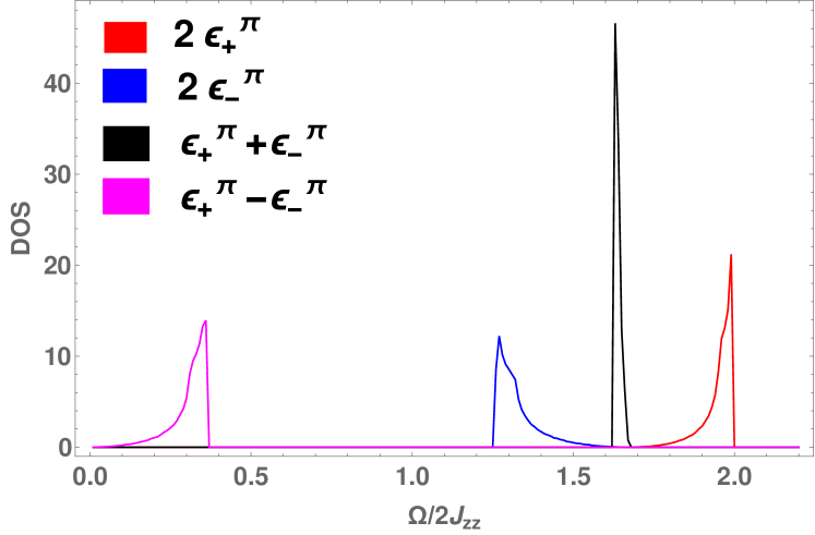
Figure 8: Density of states of different bands contributing to the phonon linewidth in the $\pi$-flux phase: We have chosen $\lambda/2J_{zz}=0.7,~{}J_{\pm}/2J_{zz}=0.3$ for illustrative purpose. Red and blue curves denote the two-particle density of states for upper($\epsilon^{\pi}_{+}$) and lower($\epsilon^{\pi}_{-}$) bands, respectively. Black and magenta curves denote density of states of $\epsilon^{\pi}_{+}+\epsilon^{\pi}_{-}$ and $\epsilon^{\pi}_{+}-\epsilon^{\pi}_{-}$, respectively.

VII.3 Beyond GMFT : Gauge fluctuations

The above Raman cross-section was obtained within GMFT neglecting the gauge fluctuations. We now consider the effect of long-wavelength gauge fluctuations within a weak-coupling approach for the emergent electrodynamics. At present, it is not clear that such a weak-coupling approach is valid for treating the gauge fluctuations. In fact the coupling parameter– the fine structure constant– for the emergent electrodynamics is generically expected to be sizeable. However, recent numerical calculations [PhysRevLett.127.117205] on quantum spin ice (via Eq. 14) suggest that the emergent fine-structure constant is $\lesssim 0.1$ which may suggest that the perturbative expansion could still provide an estimate of the effect of gauge fluctuations.

For the zero flux case, this is captured by the expansion, $e^{\pm iA_{\mathbf{r},{\bm{\mu}}}}\approx\left(1\pm iA_{\mathbf{r},{\bm{\mu}}}\right)$. Hence, (from Eq. LABEL:eq_bare_monopole_hamiltonian) the interaction between monopole and gauge field is given by,

$$H_{GF}=\frac{iJ_{\pm}}{4\sqrt{N}}\sum_{\mathbf{k,k^{\prime}},\mu\neq\nu}\Big{[} \gamma_{B}^{\mu\nu}(\mathbf{k,k^{\prime}})A_{\mathbf{k-k^{\prime}},\mu}\phi_{\mathbf{k},B}^{\dagger}\phi_{\mathbf{k^{\prime}},B}$$

$$+\gamma_{A}^{\mu\nu}(\mathbf{k,k^{\prime}})A_{\mathbf{k-k^{\prime}},\mu}\phi^{\dagger}_{\mathbf{k},A}\phi_{\mathbf{k^{\prime}},A}\Big{]}$$ (42)

where $A_{\mathbf{k},\mu}=\frac{1}{\sqrt{N}}\sum_{\mathbf{r}\in I}A_{\mathbf{r},{\bm{\mu}}}e^{i\mathbf{k}\cdot\mathbf{r}}$. The details of the vertex functions, $\gamma^{\mu\nu}_{A/B}({\bf k,k^{\prime}})$, are given in Appendix LABEL:appendix_beyond_gmft for the zero flux phase. The $\pi$-flux phase can be treated in a similar way. There are two (related by Ward identities) effects of the gauge fluctuations– renormalisation of the vertex (Fig. 2(a)) and renormalisation of the monopole propagator (Fig. 9)– which we discuss in turn.

In presence of such gauge fluctuations, the vertex functions for the bare phonon-monopole interactions get dressed via the virtual photon exchange processes as described by Fig. 2(a). This effect can be taken into account by calculating the modified vertices, $\alpha_{\bf k}^{(\rho)}+\delta\alpha_{\bf k}^{(\rho)}$. We compute the leading order corrections by expanding the bare monopole energy about the band minima at ${\bf k}=0$ (Eq. LABEL:eq_monopole_quadratic). Similarly, all the bare vertex functions ($\alpha^{(e)}_{\bf k},\alpha^{(t_{2})}_{\bf k},\gamma^{\mu\nu}_{A/B}({\bf k,k^{\prime}})$) are also Taylor expanded in polynomials of momentum and only the leading terms are considered. We note that the terms with higher powers of momentum contribute to more sub-leading (in temperature) corrections to the mean-field vertices at low temperatures. With the above approximations, the leading frequency independent corrections to the ${\bf e_{g}}$ and ${\bf t_{2g}}$ vertices are obtained as (see Appendix LABEL:appendix_beyond_gmft for further details),

$$\delta\alpha_{\bf k}^{(e)}\approx a_{0}+\frac{a_{1}}{\beta^{4}}+\frac{a_{2}e^{-\beta\Delta_{0}}}{\beta^{\frac{3}{2}}}+k^{2}\left(\frac{a_{3}}{\beta^{2}}+\frac{a_{4}e^{-\beta\Delta_{0}}}{\beta^{\frac{1}{2}}}\right)$$

$$\delta\alpha_{\bf k}^{(t_{2})}\approx\tilde{a}_{0}+\frac{\tilde{a}_{1}}{\beta^{5}}+\frac{\tilde{a}_{2}e^{-\beta\Delta_{0}}}{\beta^{2}}+k^{2}\left(\frac{\tilde{a_{3}}}{\beta^{3}}+\frac{\tilde{a_{4}}e^{-\beta\Delta_{0}}}{\beta}\right)$$ (43)

where $a_{i}$ and $\tilde{a}_{i}$ are temperature independent constants. The correction to the linewidth can now be obtained by incorporating these vertex corrections to Eq. 38. We note that such contributions do not change the dependence of the Raman response on the two-particle density of states of the monopoles. Instead, they modify the temperature dependence and overall profile of the linewidth vs frequency plots (see Fig. 7) obtained from the GMFT ansatz by renormalisation of the form factors. However, since the QSL phase is stabilised only at low temperatures, the temperature dependent vertex corrections merely give rise to a sub-leading correction to Eq. 38 as $T\rightarrow 0$.

Figure 9: Self-energy of the magnetic monopoles due to the gauge fluctuation.

Apart from the vertex corrections, the virtual photon exchange due to the gauge fluctuations also renormalises the monopole self-energy, via processes shown in Fig. 9. Such contributions renormalise the bare monopole linewidth as well as its band structure. The broadening of the linewidth is sub-leading in the low-temperature regime. On the other hand, the renormalisation of the band structure modifies the two-particle density of states of monopoles by an amount proportional to the speed of emergent light ($c_{e}$). As a result, the Raman linewidth gets renormalised compared to the GMFT results described in Fig. 7 via the dressed two-monopole density of states. However, since the large anisotropy of the exchange coupling ($J_{zz}\gg J_{\pm}$) ensures $\Delta_{0}\gg c_{e}$ [PhysRevLett.127.117205, rau2017, benton], such effects are small. The large gap of the magnetic monopoles in QSL phase preserves the essential features of the Raman response obtained in the GMFT ansatz.

VIII Self-energy of the phonon due to phonon-photon coupling

Similar to the Raman response due to the phonon-monopole coupling, the leading contribution to the phonon linewidth due to phonon-photon interaction (see Eq. 24) can be computed from the Feynman diagram shown in Fig. 10 appearing in the second-order perturbation theory. The phonon self-energy is given by,

Figure 10: Self-energy of the phonon due to the phonon-(emergent) photon interaction (see Fig. 2(b)).

$$\Sigma_{\zeta^{(e)}}({\bf q},i\Omega)=\frac{1}{\beta^{2}}\sum_{\bf k_{2},k_{3},k_{4}}\sum_{\Omega_{2}\Omega_{3}\Omega_{4}}\mathcal{G}^{\beta\gamma}({\bf q,k_{2},k_{3},k_{4}}) \mathcal{G}^{\mu\nu}({\bf q,k_{2},k_{3},k_{4}})\delta(\Omega+\Omega_{2}+\Omega_{3}+\Omega_{4})$$

$$\times~{}G_{\zeta}({\bf k_{2}},\Omega_{2})D_{\beta\mu}({\bf k_{3}},\Omega_{3})D_{\gamma\nu}({\bf k_{4}},\Omega_{4})\delta({\bf q+k_{2}+k_{3}+k_{4}})$$ (44)

Here $D_{\mu\nu}({\bf q},i\omega)$ denotes the photon propagator which can be calculated from the effective low-energy Hamiltonian of the pure gauge theory given in Eq. 14, i.e.,

$$D_{\mu\nu}({\bf q},i\omega) =-\int_{0}^{\beta}d\tau\langle\hat{\mathcal{T}}\left(A_{{\bf q},\mu}(\tau)A_{{\bf-q},\nu}(0)\right)\rangle e^{i\omega\tau}$$

$$=-\frac{U\delta_{\mu\nu}}{\omega^{2}+\varepsilon_{\bf q}^{2}}$$ (45)

Eq. 44 can be further simplified by performing the frequency summation [mahan]. For the Raman scattering experiments discussed earlier, we consider only the ${\bf q}\rightarrow 0$ limit and focus on the imaginary part. Typically, the dispersion for the optical phonon can be approximated as, $\omega_{\bf q}\rightarrow\omega_{0}$. Also, the energy scale of the emergent photon is much smaller than the optical phonon excitations of the pyrochlores [moon, rau2017, natalia2021]. Hence, at the low temperatures of the QSL phase, it is fair to consider $n(\omega_{0})\ll n(\varepsilon_{\bf k})$. Setting $n(\omega_{0})=0$ in the leading approximation, the contribution to the phonon linewidth is obtained as,

$$\Gamma(0,E)=\frac{\pi(J_{ph-ph}U)^{2}}{2N^{2}}\sum_{\bf k}\left[{\bf k\cdot k}\delta_{\beta\gamma}-k^{\beta}k^{\gamma}\right]^{2}~{}\frac{1}{4\varepsilon_{\bf k}^{2}}\bigg{[}\delta({E+\varepsilon_{\bf k}})~{}[n(-E)]^{2} +\delta({E-\varepsilon_{\bf k}})~{}[1+n(E)]^{2}$$

$$+\delta(E)~{}\left\{2[n(\varepsilon_{\bf k})][n(\varepsilon_{\bf k})+1]\right\}\bigg{]}$$ (46)

where, $E=(\Omega-\omega_{0})/2$. It is clear from the above expression that the Raman response occurs around $\Omega=\omega_{0}$ due to the gaplessness of the photons, which is different from the frequency window at which the magnetic monopole signatures occur. For small positive energies $E$, the above expression is further simplified to,

$$\Gamma(0,E)\propto E^{4}(1+n(E))^{2}$$ (47)

For the higher energy regime, the photon band structure starts deviating from the linear behaviour and the above form is no longer valid. The complete energy dependence of the above contribution to the linewidth is shown in Fig. 11 for different temperatures, where we have used the lattice regularized dispersion for the emergent photons [rau2017, benton]. Apart from the usual dipolar form factor, the linewidth profile is mostly sensitive to the photon density of states, which is shown in the inset of Fig. 11.

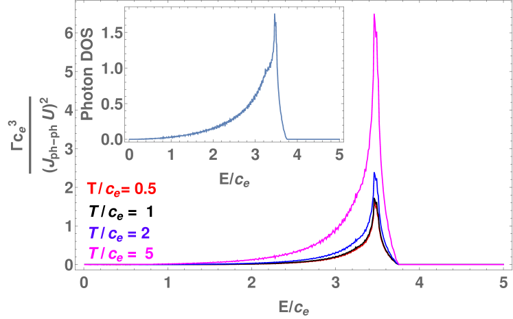
Figure 11: Energy dependence of the linewidth of the $\mathbf{e_{g}}$ phonons due to phonon-(emergent) photon coupling: The energy dependence is shown at different temperatures. $c_{e}=\sqrt{UK}$ is the velocity of the emergent photons and its density of states is plotted in the inset.

IX Self-energy of the phonon due to phonon-electric charge coupling

The final contribution to the phonon self-energy in the QSL phase arises from scattering of the phonons off the electric charges. Again, assuming weak coupling between the charges and the gauge field, we compute the phonon linewidth due to Eq. 26 using GMFT. As we have already seen, this interaction is very similar to that between phonons and monopoles. Hence, the contribution to the phonon self-energy also comes from similar Feynman diagrams as shown in Fig. 12. There are two possible scattering channels for electric charge-phonon interactions– absorption of a phonon by a charge, or, annihilation of a phonon followed by pair production of charges (with charge $\pm 1$). Similar to monopoles, only the second process is relevant here. Therefore, $\Gamma\sim\Theta(\mid\Omega\mid-2\Delta_{c})$, and the linewidth vs frequency profile closely follows the two-particle density of states of the electric charges. This is shown in Fig. 13 for $t/m=0.2$ as an illustrative example (However, it can be chosen from any value that satisfies, $m>2\sqrt{2}t$, defining the validity of the QSL description, and the profile remains qualitatively unchanged). Clearly, the Raman response due to the phonon-charge coupling has a threshold energy scale of $\sim 2\Delta_{c}$ which is a different energy scale compared to the response due to magnetic monopoles and photons.

Figure 12: Self-energy of the phonon due to the phonon-electric charge interaction (see Fig. 5)

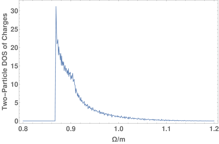
Figure 13: Two-particle density of states of the charges: For illustrative purpose, we have chosen $t/m=0.2$ where $\Delta_{c}/m=0.43$.

X Bilinear coupling

Having discussed the effects of the linear magnetoelastic coupling in the QSL phase, we now briefly discuss the more familiar contribution to the Raman response of the phonons arising due to magnetoelastic interaction. This is present both in Kramers and non-Kramers systems, as it arises due to modulation of the spin-exchange interactions via the phonons and can be obtained from the bare spin Hamiltonian of Eq. 3 by Taylor expanding the exchange coupling constants in powers of lattice displacements ($\bm{\delta_{\mu\nu}}$) from the ionic equilibrium position ($\mathbf{\bar{R}}_{\bm{\mu\nu}}$) [cdcro] as

$$J^{\mu\nu}_{\alpha}({\bf r})=J_{\alpha} +\frac{\partial J^{\mu\nu}_{\alpha}({\bf r})}{\partial R^{a}_{\mu\nu}}\delta^{a}_{\mu\nu}({\bf r})$$

$$+\frac{1}{2}\frac{\partial^{2}J_{\alpha}^{\mu\nu}({\bf r})}{\partial R^{a}_{\mu\nu}\partial R^{b}_{\mu\nu}}\delta^{a}_{\mu\nu}({\bf r})\delta^{b}_{\mu\nu}({\bf r})$$ (48)

Here, $J^{\mu\nu}_{\alpha}({\bf r})$ denotes the generic bond dependent exchange coupling constant on the bond of the pyrochlore connecting the sites $({\bf r},\bm{\mu})$ and $({\bf r},\bm{\nu})$. Here, $(\mathbf{r},{\bm{\mu}})$ denotes the position vector of the four spins sitting on the corners of the tetrahedron with its centre at $\mathbf{r}$ for $\mu=0,1,2,3$, with $\alpha$ representing $zz$ or $\pm$ interactions, and,

$$R^{a}_{\mu\nu}=(\mathbf{r},{\bm{\mu}})^{a}-(\mathbf{r},{\bm{\nu}})^{a},\indent(a=x,y,z)$$

$$\delta^{a}_{\mu\nu}=R^{a}_{\mu\nu}-\bar{R}^{a}_{\mu\nu}$$

Substituting Eq. 48 in the spin-Hamiltonian of Eq. 3, we get the coupling between the phonons and spin-bilinears,

$$H^{quad}_{sp}=H_{1}+H_{2}$$ (49)

where $H_{1}$ and $H_{2}$ represent the interaction vertices linear and quadratic in phonons, respectively. Their detailed forms are given by Eq. LABEL:eq_quadratic_spin_phonon_coupling_1 and LABEL:eq_quadratic_spin_phonon_coupling_2 in Appendix LABEL:appendix_quadratic. A unitary transformation can be performed on the displacement operators, $\bm{\delta}_{\mu\nu}(\mathbf{r})$, to re-write it in the normal mode coordinates, $\bm{\zeta}^{(\rho)}(\mathbf{r})$, described in Sec. III. The above interaction is re-written in terms of the fractionalised degrees of freedom in a QSL phase using the parton decomposition of spins as described in Sec. IV. Within GMFT, the quadratic magnetoelastic coupling between the phonons and emergent excitations of the QSL is described by Fig. LABEL:fig_phonon_monopole_interaction_quad and LABEL:fig_phonon_photon_interaction_quad (also see Eq. LABEL:eq_quadratic_qsl_1 and LABEL:eq_quadratic_qsl_2 in Appendix LABEL:appendix_quadratic).

The phonon-magnetic monopole vertex arising from the quadratic coupling is shown in Fig LABEL:fig_phonon_monopole_interaction_quad where (a) and (b) panels show the contribution from $H_{1}$ , and, (c) and (d) panels show the contribution from $H_{2}$. It is clear from these diagrams that such magnetoelastic coupling gives rise to the hopping of the monopoles which preserves the monopole flavour, i.e., monopoles on A and B sublattices do not mix under this dynamics. This feature can be contrasted with the monopole dynamics due to the linear magnetoelastic coupling described earlier in Eq. 20 and 21.