The evolution of the heaviest super-massive black-holes in jetted AGNs

Abstract

We present the space density evolution, from z=1.5 up to z=5.5, of the most massive (M$\geq 10^{9}$M_☉) black holes hosted in jetted Active Galactic Nuclei (AGNs). The analysis is based on a sample of 380 luminosity-selected ($\lambda$L${}_{1350}\geq 10^{46}$ erg s^-1 and P${}_{5\text{GHz}}\geq 10^{27}$ W Hz^-1) Flat Spectrum Radio Quasars (FSRQs) obtained from the Cosmic Lens All Sky Survey (CLASS). These sources are known to be face-on jetted AGNs (i.e. blazars) and can be exploited to infer the abundance of all the (misaligned) jetted AGNs, using a geometrical argument. We then compare the space density of the most massive SMBHs hosted in jetted AGNs with those present in the total population (mostly composed by non-jetted AGNs). We find that the space density has a peak at $z\sim 3$, which is significantly larger than the value observed in the total AGN population with similar optical/UV luminosities ($z\sim 2.2$), but not as extreme as the value previously inferred from X-ray selected blazars ($z\gtrsim 4$). The jetted fraction (jetted AGNs/total AGNs) is overall consistent with the estimates in the local Universe (10–20%) and at high redshift, assuming Lorentz bulk factors $\Gamma\approx 5$. Finally, we find a marginal decrease in the jetted fraction at high redshifts (by a factor of $\sim 2$). All these evidences point toward a different evolutionary path in the jetted AGNs compared to the total AGN population.

1 Introduction

Studying how Super-Massive Black Holes (SMBHs) have evolved across cosmic time is a fundamental step for our comprehension of the formation and evolution of the cosmic structures in the Universe. According to the current paradigm, the growth of the SMBH should happen during the process of accretion on a massive black hole seed present in the centre of a galaxy (e.g. Merloni, 2016 for a comprehensive review). Since the accretion is also the basis of the AGN phenomenon, tracing the evolution of the AGN phase represents the most compelling way to study the SMBHs growth, especially at high redshifts (e.g. Volonteri, 2010; Valiante et al., 2017). Particularly important is to establish the possible role of relativistic jets in this process (for a recent review on the relativistic jets in AGNs see Blandford et al., 2019). These powerful and collimated jets are able to produce strong radio emission and hence the jetted AGNs are usually referred as radio-loud (RL, e.g. Best & Heckman, 2012). If the presence of a jet is the consequence of a rapidly spinning black hole (e.g. Tchekhovskoy et al., 2011; Narayan et al., 2014), we expect that RL AGNs should be very effective in transforming accreting mass into energy (Tchekhovskoy et al., 2011; Narayan et al., 2014). A pure general relativity estimate results in a radiation efficiency of $\eta\sim 0.3$ for a maximal rotating BH and $\eta\sim 0.1$ for a non-rotating BH (e.g. Thorne, 1974). Therefore the black hole mass-growth in RL AGNs should be on average significantly slower compared to non-jetted, or radio-quiet (RQ), AGNs. As a consequence, we expect the most massive SMBHs hosted in RL to be less abundant at high redshift than those hosted in the RQ counterpart, assuming that RL AGNs remain that way through all their accretion episodes. Evidence supporting this prediction, however, has not been found yet. On the contrary, several studies have shown no clear dependence on the ratio of RL to RQ AGNs with redshift (e.g. Stern et al., 2000; Bañados et al., 2015; Liu et al., 2021) while other studies indicate that RL AGNs with the most massive SMBHs ($\geq 10^{9}$ M_☉) show a more rapid evolution, peaking earlier (z$\gtrsim$4; e.g. Ajello et al., 2009; Sbarrato et al., 2015) than those hosted in RQ AGNs (peaking at z$\sim$2, e.g. Hopkins et al., 2007; Shen et al., 2020).

Establishing if SMBHs hosted in jetted AGNs followed a different evolutionary path compared to those hosted by non-jetted AGNs is not simple. The presence of a relativistic jet is usually inferred from the detection of a strong radio emission that reveals the radio-loud nature of an AGN (e.g. Urry & Padovani, 1995). A major problem, however, is that in RL AGNs the radio emission produced by the jet is strongly dependent to the viewing angle, due to relativistic beaming, and, therefore, the same source will show a different value of radio-loudness (defined as the rest-frame radio-to-optical luminosity ratio, Kellermann et al., 1989) depending to its actual orientation. This is particularly true at high radio frequencies where the emission is almost completely dominated by the beamed part of the radio emission (the jet). In this respect, high-z AGNs could be very problematic since the typical observing radio frequencies (1.4–5 GHz) correspond to very high rest-frame frequencies (8–30 GHz for a z=5 AGN). In addition, the extended (and more isotropic) radio emission from the radio-lobes of RL AGNs could be heavily damped at high-z due to the increasing density of photons from the Cosmic Microwave Background (CMB) that interact and cool the relativistic electrons responsible for the radio emission (Ghisellini et al., 2014a). Finally, as in radio-quiet AGNs, obscuration of the optical/UV radiation, due to the molecular torus, makes the detection of an important fraction of sources (the so-called type-II AGNs) at high-z very challenging (e.g. Vito et al., 2018). All these observational issues can introduce relevant selection effects in all the estimates of the number of jetted AGNs at different cosmic epochs that are difficult to quantify.

A possible way out is to focus only on the sources that are seen at small angles from the jet direction, i.e. on blazars (see e.g. Volonteri et al., 2011; Sbarrato et al., 2015). Knowing that a blazar is typically observed at a viewing angle of $\theta\lesssim 1/\Gamma$, where $\Gamma$ is the Lorentz factor of the bulk velocity in the jet, we can effectively use these objects to estimate the space density of all jetted AGNs in a region of Universe, with a purely geometrical argument. Specifically, the total number of jetted AGNs (N${}_{\text{jet}}$) in a given volume of Universe is expected to be: $N_{\text{jet}}\approx 2\Gamma^{2}N_{\text{blazar}}$ i.e. there are about 200 RL AGNs for each observed blazar, assuming a typical $\Gamma=10$ (e.g. Ghisellini et al., 2014b). Another great advantage of this method is that the powerful jet is thought to wipe out the material along its path in the AGNs earlier stage, and hence obscuration effects are expected to be negligible. This makes the identification and the characterization of the optical counterpart more efficient and reliable. Therefore, from the estimate of the blazar space density it is possible to derive, in principle, a complete census of the entire jetted AGNs population without the biases due to radio emission anisotropy and to obscuration.

The application of this method requires the existence of flux-limited and statistically complete samples of blazars. In this paper we will use the Cosmic Lens All Sky Survey (CLASS, Myers et al., 2003; Browne et al., 2003) to build one of the largest radio flux limited samples of blazars covering a large fraction of the sky ($\sim 16300\text{ deg}^{2}$) and that includes sources up to z$\sim$5.5. In particular, we are interested in tracing the evolution of the most massive SMBHs ($\geq$10⁹ M_☉) where a large difference in the evolutionary properties has been recently reported (e.g. Ajello et al., 2009; Ghisellini et al., 2010; Volonteri et al., 2011; Sbarrato et al., 2015). Although for some objects in our sample the estimate of the SMBH masses is present in the literature (e.g. Shen et al., 2011) all the masses are recomputed here following a single coherent method. In this way our analysis should be free from possible biases that can derive from using different techniques (or emission lines) for sources located at different redshifts.

The paper is organized as follow. In Sect. 2 we describe the selection process of our luminosity-limited sample. In Sect. 3 we describe the analysis of the spectra and the estimation of the relevant parameters, furthermore we discuss the potential issues that could affect our estimates. In Sect. 4 we derive the number density of SMBHs with M$\geq 10^{9}$M_☉ hosted in blazars and in all the jetted AGNs. In Sects. 5 and 6 we discuss the results and we draw our conclusions. Throughout the paper we assume a flat $\Lambda$CDM cosmology with H${}_{0}=70$ km s^-1Mpc^-1, $\Omega_{\lambda}=0.7$ and $\Omega_{\text{M}}=0.3$.

2 The Sample

We start our selection from the CLASS, a radio survey at 5 GHz of flat-spectrum radio sources that covers most of the northern sky ($16300\ \text{deg}^{2}$) and that contains $\sim 11000$ sources. This catalogue was built by combining the NRAO Very Large Array Sky Survey (NVSS), at 1.4 GHz (Condon et al., 1998), with the Green-Bank Survey (GB6) at 5 GHz (Gregory et al., 1996) and by selecting only the objects with a flat spectrum between 1.4 and 5 GHz ($\alpha<0.5$, with $f_{\nu}\propto\nu^{-\alpha}$) with a final follow-up at 8.4 GHz using the Very Large Array (VLA) in the largest configuration (A), that granted an angular resolution of $\sim 0.2\arcsec$. The sub-arcsecond accuracy of the radio sources positions proved to be crucial to find the correct optical counterpart, in particular at faint magnitudes. Since blazars are flat-spectrum radio sources, CLASS represents the most efficient and reliable starting point to select a radio flux-limited sample of these sources suitable for statistical analyses.

We have recently carried out a specific search for blazars with redshift above 4 in the CLASS survey by efficiently pre-selecting candidates from the The Panoramic Survey Telescope and Rapid Response System (Pan-STARRS1, PS1, Chambers et al., 2016), using the so-called drop-out technique (see Caccianiga et al., 2019 for details). Nearly all the candidates with a magnitude brighter than 21 (in the r, i or z filter, depending on the expected redshift of the source) have been spectroscopically confirmed, producing a list of 25 z$\geq$4 AGNs. The spectroscopic data are gathered from the Sloan Digital Sky Survey (SDSS, Blanton et al., 2017; SDSS-I/II and the Baryon Oscillation Spectroscopic Survey, BOSS; R=1500 at $\lambda=3800$Å and R=2500 at $\lambda=9000$Å) when available, or from dedicated observations using the Multi-Object Double Spectrograph (MODS) of the Large Binocular Telescope (LBT) with the red grating (G670L, 5000-10000Å; R=2300 at $\lambda=7600$Å), or with the Telescopio Nazionale Galileo (TNG) coupled with the Device Optimized for the LOw RES-olution (DOLORES, using the LR-R/LR-B grisms; respectively, R=450 at $\lambda=4500$Å and R=360 at $\lambda=7500$Å), as detailed in Caccianiga et al. (2019). The analysis of the radio spectra (Caccianiga et al., 2019) and of the X-ray data (Ighina et al., 2019, 2021) have then confirmed the blazar nature for 22 of these objects. If we restrict the search area to the high Galactic latitudes ($|b\arcsec|\geq 20\text{ deg}$) where the identification level is close to 100%, 3 out of 22 blazars are excluded. The resulting 19 objects constitute the high-z complete sample, hereafter C19, with a sky coverage area of 13120 deg².

To extend this sample at lower redshifts (1$<$z$<$4) we have considered the CLASS sources falling in the sky area covered by the SDSS Data Release 14 (DR14, Abolfathi et al., 2018) in order to benefit of the large spectroscopic database available for most of the brightest objects. Since we are interested in the most massive SMBHs, that are hosted in the most luminous AGNs, the SDSS spectroscopic data are deep enough to obtain a sample with a high spectroscopic identification level. We have thus cross-correlated CLASS with the SDSS DR14 photometric catalogue using a 1$\arcsec$ positional tolerance to guarantee that all the counterparts are recovered (see below). We have found a counterpart for about 74% of the CLASS sources in the SDSS area (6244 out of 8389). We have then verified that the large majority (95%) of these counterparts have a distance from the CLASS position less than 0.3$\arcsec$ thus confirming the high completeness of the radio/optical association. About 50% of the counterparts have a spectroscopic identification. This fraction, however, dramatically increases when considering the brightest sources, leading to a high identification level of the final sample, as explained below.

In order to select sources with the same radio and optical luminosities as in the C19, we can translate the radio and optical flux limits of the high-z sample of C19 (m${}_{\text{AB}}\leq 21$ and S${}_{\text{5GHz}}\geq 30\ \text{mJy}$) into luminosity lower limits at lower redshifts, assuming a starting redshift of z=4, namely:

$$\lambda\text{L}_{\lambda}(1350\text{\AA})\gtrsim 10^{46}\ \text{erg}\ \text{s}^{-1}$$ (1)

$$\text{P}_{\text{5GHz}}\gtrsim 10^{27}\ \text{W}\ \text{Hz}^{-1}$$ (2)

We also decided to consider only sources with z>1.5. The main reason for this choice is that the inclusion of lower redshift objects in the analysis would have required to consider an additional emission line for the SMBH estimate (i.e. H$\beta$, if CIV1549Å is not visible; see Section 3 for details). The use of multiple emission lines may introduce some systematic that can affect the final results. In any case, our goal is to better sample the redshift range between 2 and 4 where the blazar space density is expected to peak and, therefore, excluding sources below z=1.5 does not affect our analysis. We also exclude the objects with z$\geq$4, that are already included in the C19 part of the sample.
As mentioned above, we want to analyse a FSRQ sample, hence we exclude BL Lac objects. Finally, we exclude the objects with low Galactic latitude (|b$\arcsec|<20$), by analogy with the selection of C19. The resulting 1.5$<$z$<$4 sub-sample contains 361 objects, with a sky coverage area $\sim 10700\ \text{deg}^{2}$.

We have then evaluated the completeness of this sample. As mentioned above, not all the CLASS sources in the SDSS area are spectroscopically identified in the literature. We worked out a correction to account for the missing sources.

As a first step, we split the sample in 8 bins of redshift. Then, we have translated the radio and optical flux limits of the high-z sample of C19, starting from redshift z=4, at lower redshifts, using the following relations:

$$\text{mag}_{r}\text{(z)}=20.86+5\text{Log}\left(\frac{\text{D}_{\text{L}}\text{(z)}}{\text{D}_{\text{L}}(4)}\right)+2.5(\alpha_{\text{O}}-1)\cdot\text{Log}\left(\frac{1+\text{z}}{1+4}\right)$$ (3)

$$\text{S}_{\text{5GHz}}\text{(z)}=30\left(\frac{\text{D}_{\text{L}}(4)}{\text{D}_{\text{L}}\text{(z)}}\right)^{2}\left(\frac{1+4}{1+\text{z}}\right)^{(\alpha_{\text{R}}-1)}\text{mJy}$$ (4)

where mag${}_{\text{r}}$(z) is the Galactic-extinction corrected PS1 magnitude limit in the r-filter and S${}_{\text{5GHz}}$(z) is the radio flux density limit (at 5 GHz) at redshift $z$; 20.86 is the magnitude limit used in the C19 sample (21th magnitude) corrected for the average Galactic Extinction of the C19 sample; D${}_{\text{L}}$(z) is the luminosity distance at redshift $z$; $\alpha_{\text{O}}$ and $\alpha_{\text{R}}$ are the optical and radio spectral indices respectively. In particular, assuming $S(\nu)\propto\nu^{-\alpha}$ we use $\alpha_{\text{O}}=0.44$ (Vanden Berk et al., 2001) and $\alpha_{\text{R}}=0$. The Eqs. 3 and 4 are equivalent to Eqs. 1 and 2, and represent de facto a luminosity selection.
We can therefore compute the radio and optical flux limits, using the value of redshift in the centre of each bin. We then compute the identification level for each bin, as the fraction of the CLASS sources above these limits in the SDSS sky area with a spectroscopic identification in the literature. The inverse of this number gives the multiplicative factor ($C_{\text{id}}$) to correct for the identification level. This correction range from 1.16 (at low redshifts) to 1.45, at redshift $\sim$3.5.

Moreover, some spectroscopically identified objects present in the literature lack a SDSS spectrum. For these objects we are not able to estimate the mass of the central BH. Nevertheless, under the assumption that all these blazars (either with spectrum or not) share the same properties, we can take into account the missing spectra with a second correction. Similarly to the $C_{\text{id}}$, we calculate this correction for each bin of redshift, specifically we compute the fraction of objects with a spectrum available from SDSS, and included in the CLASS, in each redshift bin and the correction is defined as the inverse of this number (hereafter, $C_{\text{spect}}$). The correction ranges from 1.02 to 1.15. In Tab 1 we report the values of $C_{\text{id}}$ and $C_{\text{spect}}$ for each redshift bin.

The uncertainties on these coefficients are evaluated assuming a binomial distribution $B(N,p)$, where N is the total number of sources in each bin of redshift for the considered correction, and $p$ is the inverse of the true correction. Specifically, we are interested here in the compound uncertainty obtained by multiplying the two corrections. We evaluate, through a Monte Carlo simulation, that the impact of these statistical uncertainties on the final result are at most $\sim 6\%$.

Using these corrections we can obtain a reliable estimate of the actual number of blazars expected in each redshift bin.
For the z$>$4 sub-sample these correction are not necessary since the identification level is almost 100% (see C19 for details).

2.1 Confirming the blazar nature

By definition, the CLASS survey should only contain sources with a flat spectrum (i.e. blazars) between 1.4 and 5 GHz. However, since the spectral index estimate is based on two frequencies only, other AGNs with more complex radio spectra may be included in the CLASS. This is the case for Gigahertz Peaked Spectrum (GPS) sources, which are thought to be young and compact AGNs and that show a peak in the radio spectrum at high frequencies (1–5 GHz, O’Dea, 1998). If the peak falls in the observed 1.4–5 GHz range, the corresponding source can be misinterpreted as a FSRQ. We expect that most of the sources with a GPS spectrum are not oriented sources, i.e. blazars. In order to confirm the blazar nature of the CLASS sources, we considered their X-ray properties, which can be used as an independent and reliable proxy to assess the presence of relativistic beaming (e.g. Ghisellini, 2015, Ighina et al., 2019). Indeed, an X-ray emission significantly higher than that expected from a RQ AGN with the same optical/UV luminosity is a robust evidence of the presence of an extra emission coming from an oriented relativistic jet.

To this end, we collected X-ray data from the second Swift-XRT point sources catalog (2SXPS, Evans et al., 2020). We found 107 detections (35% of the sample). After combining the X-ray fluxes with the optical properties from SDSS, we compute the $\tilde{\alpha}_{ox}$ parameter for all these AGNs. We find that the large majority of these sources ($\sim 94-96\%$, depending on the assumption on the photon index, $\Gamma$=1.5–1.8) are strong X-ray emitters in the typical range observed in blazars ($\tilde{\alpha}<$ 1.355, see e.g. Ighina et al., 2019).
It should be noted that the $\sim$100 CLASS sources detected in the 2SXPS catalog could not be representative of the entire sample. Indeed, the 2SXPS catalogue is based on archival pointed data and, therefore, blazars could be over-represented since they have been preferentially pointed by Swift-XRT. To avoid this possible bias, we also considered in the computation only the sources that are serendipitously detected by Swift-XRT, i.e. sources that were not specifically pointed. Using this sample, that contains 24 sources, we confirm a similar abundance of blazars (i.e. $\sim 92-96\%$). We note that these results are consistent with what found in the z>4 C19 sample, where about 90% of radio selected candidates were confirmed as blazars using the X-rays data (Ighina et al., 2019). We expect this fraction is representative of the whole sample, including the sources not yet observed in the X-rays, and, therefore, we apply a scale correction to the low-redshift (z<4) blazar density calculated in Section 4 to take into account the presence of this small fraction (6%) of non-blazars sources, in the sample.

z bin	S${}_{\text{5GHz}}$	m${}_{\text{AB}}$	C${}_{\text{id}}$	C${}_{\text{spect}}$
1.50 - 1.75	140	18.88	1.16	1.14
1.75 - 2.00	108	19.21	1.18	1.09
2.00 - 2.25	86	19.49	1.22	1.09
2.25 - 2.50	71	19.74	1.26	1.08
2.50 - 2.75	60	19.96	1.31	1.02
2.75 - 3.00	51	20.16	1.34	1.05
3.00 - 3.50	42	20.42	1.39	1.08
3.50 - 4.00	33	20.72	1.45	1.15

Table 1: Values of C${}_{\text{id}}$ and C${}_{\text{spect}}$ for different redshift bins (z<4 sub-sample). column 1: redshift interval; column 2 and 3: respectively, lower radio-flux (mJy) limit and lower magnitude limit calculated at the central redshift of each bin (see Eqs. 3, 4); column 4 and 5: Multiplicative factors that correct for the missing identification of the sample and for the lack of SDSS spectra, respectively.

3 Estimating the masses of the SMBHs

One of the most used and reliable method to calculate the mass of the central SMBH in type-I AGNs, is based on the virial theorem applied to the Broad Line Region (BLR). Assuming a completely virialized BLR we can compute the mass of the central BH from the BLR size and from the velocity dispersion of the orbiting clouds that form it:

$$M_{\text{BH}}=f\frac{{R_{\text{BLR}}\Delta V}^{2}}{G}$$ (5)

Where $\Delta V$ is a measure of the velocity dispersion of the BLR clouds, and $R_{\text{BLR}}$ is a measure of the BLR size. f is a dimensionless factor that depends on the structure and the geometry of the BLR (e.g., Vestergaard & Peterson, 2006, hereafter VP06).
The Doppler broadening of the line provides the necessary information about the velocity dispersion of the ionized gas where the lines are produced. The BLR radius, instead, can be inferred from the continuum (or the line) luminosity using scaling relations of the form of $R\propto L^{\kappa}$ (e.g., Kaspi et al., 2000; Grier et al., 2019). This relationship can therefore be used to estimate the radius of the BLR from a single luminosity measure, without the need of a continuous monitoring of the source. For this reason, this method is called single epoch (SE).
Among all the possible Broad Emission Lines (BELs), just a few of them are strong enough to be used for a reliable estimate of the BH mass: H$\beta\lambda 4861$, MgII$\lambda 2799$ and CIV$\lambda$1549 are the most studied and used (e.g. Vestergaard & Peterson, 2006; Shen & Liu, 2012; Bentz, 2015). With an AGN sample that covers a large range of redshift, the natural choice among the aforementioned three is the triply ionized carbon line (CIV$\lambda$1549). Even though there are some concerns about the use of this line to estimate the SMBH masses (see Subsection 3.3 for a discussion of these potential issues), we decide to use this line since it is observable from z$\sim$1.5 up to z$\sim$5.5 in an optical spectrum and, therefore, it can be consistently used for the entire sample. This is a great advantage with respect of using different emission lines (or even different methods) depending on the redshift, something that can introduce unpredictable biases in the analysis of the space density versus z.

There are different ways to quantify the line width, the most common one being the Full Width at Half Maximum (FWHM). However, several authors (e.g. Vestergaard & Peterson, 2006; Denney et al., 2013) suggest that the $\sigma_{l}$ (line dispersion) can give more reliable results for the BH mass estimate. For instance, by comparing the CIV based masses with those derived with other independent methods, Denney et al. (2013) has concluded that the line dispersion can lead to BH masses with a lower scatter (<0.3 dex) if compared to FWHM, provided that high quality spectra (S/N $\gtrsim$ 10) are used. We decide to compute the BH mass using both the line dispersion and the FWHM, to facilitate the comparison with the literature. In particular, we use the two relations derived by Vestergaard & Peterson (2006):

$$M_{\text{BH}}(CIV)=10^{6.66}\left(\frac{FWHM(CIV)}{10^{3}\ \text{km s}^{-1}}\right)^{2}\left(\frac{\lambda L_{\lambda}(1350\text{\AA})}{10^{44}\ \text{erg s}^{-1}}\right)^{0.53}$$ (6)

$$M_{\text{BH}}(CIV)=10^{6.73}\left(\frac{\sigma_{l}(CIV)}{10^{3}\ \text{km s}^{-1}}\right)^{2}\left(\frac{\lambda L_{\lambda}(1350\text{\AA})}{10^{44}\ \text{erg s}^{-1}}\right)^{0.53}$$ (7)

where the line dispersion and the FWHM are measured in km s^-1 and $\lambda$L${}_{\lambda}(1350\text{\AA})$ is the continuum luminosity at $1350\text{\AA}$ (source rest-frame) measured in erg s^-1. The intrinsic scatter of these relations is 0.3–0.4 dex (see Vestergaard & Peterson, 2006) and it represents the main source of uncertainty in the mass estimate.

name	z	AV	r-mag	S${}_{\text{5GHz}}$	$\sigma_{l}$	FWHM	Log$\lambda$L1350	LogLCIV	LogL${}_{\text{bol}}$	LogMσ	LogM${}_{\text{FWHM}}$	Log$\lambda_{\text{Edd}}$	Log$\lambda_{\text{Edd}}$
				(mJy)	(km s-1)	(km s-1)	(erg s-1)	(erg s-1)	(erg s-1)	(M☉)	(M☉)	[$\sigma_{l}$]	[FWHM]
GB6J001115+144608	4.96	0.242	19.62	31	$3310\pm 138$	$7548\pm 322$	$47.326\pm 0.004$	$45.240\pm 0.012$	$47.979\pm 0.004$	$9.53\pm 0.04$	$10.18\pm 0.04$	$0.35\pm 0.04$	$-0.30\pm 0.04$
GB6J012202+030951	4.00	0.161	20.86	96	-	$5800\pm 2000$	$46.450\pm 0.070$	-	$47.103\pm 0.070$	-	$9.52\pm 0.39$	-	$-0.51\pm 0.39$
GB6J083548+182519	4.41	0.141	21.18	40	$2191\pm 89$	$5032\pm 211$	$46.104\pm 0.029$	$44.497\pm 0.016$	$46.757\pm 0.029$	$8.53\pm 0.04$	$9.18\pm 0.04$	$0.13\pm 0.04$	$-0.52\pm 0.04$
GB6J083945+511206	4.40	0.175	19.37	51	$5463\pm 119$	$5806\pm 280$	$46.795\pm 0.005$	$45.103\pm 0.007$	$47.448\pm 0.005$	$9.69\pm 0.02$	$9.67\pm 0.04$	$-0.34\pm 0.02$	$-0.32\pm 0.04$
GB6J090631+693027	5.47	0.204	20.54	100	-	-	-	-	-	$9.30\pm 0.39$	$9.30\pm 0.39$	-	-
GB6J091825+063722	4.22	0.163	19.86	36	$3031\pm 109$	$6967\pm 266$	$46.702\pm 0.009$	$44.782\pm 0.014$	$47.355\pm 0.009$	$9.13\pm 0.03$	$9.78\pm 0.03$	$0.13\pm 0.03$	$-0.52\pm 0.03$
GB6J102107+220904	4.26	0.095	21.21	108	$3751\pm 357$	$3097\pm 325$	$46.007\pm 0.026$	$44.562\pm 0.015$	$46.660\pm 0.026$	$8.94\pm 0.08$	$8.71\pm 0.10$	$-0.38\pm 0.08$	$-0.15\pm 0.09$
GB6J102623+254255	5.28	0.079	21.95	142	$4183\pm 488$	$5613\pm 510$	$46.692\pm 0.011$	$45.144\pm 0.022$	$47.345\pm 0.011$	$9.40\pm 0.10$	$9.58\pm 0.08$	$-0.16\pm 0.10$	$-0.34\pm 0.08$
GB6J132512+112338	4.42	0.105	19.41	62	$3463\pm 82$	$3484\pm 356$	$46.568\pm 0.008$	$45.208\pm 0.011$	$47.221\pm 0.008$	$9.17\pm 0.02$	$9.10\pm 0.10$	$-0.05\pm 0.02$	$0.02\pm 0.10$
GB6J134811+193520	4.40	0.098	20.73	38	$5359\pm 280$	$4838\pm 247$	$46.337\pm 0.013$	$44.609\pm 0.012$	$46.990\pm 0.013$	$9.43\pm 0.05$	$9.27\pm 0.05$	$-0.54\pm 0.05$	$-0.38\pm 0.04$
GB6J141212+062408	4.47	0.110	20.23	34	$3052\pm 313$	$7161\pm 749$	$46.494\pm 0.015$	$44.252\pm 0.020$	$47.147\pm 0.015$	$9.02\pm 0.08$	$9.69\pm 0.09$	$0.03\pm 0.08$	$-0.65\pm 0.09$
GB6J143023+420450	4.71	0.058	21.00	337	$3541\pm 186$	$8129\pm 450$	$46.627\pm 0.011$	$44.602\pm 0.014$	$47.280\pm 0.011$	$9.22\pm 0.05$	$9.87\pm 0.05$	$-0.04\pm 0.05$	$-0.69\pm 0.05$
GB6J151002+570256	4.31	0.078	20.34	292	$2540\pm 113$	$2322\pm 272$	$46.532\pm 0.010$	$44.830\pm 0.014$	$47.185\pm 0.010$	$8.88\pm 0.04$	$8.73\pm 0.11$	$0.20\pm 0.04$	$0.35\pm 0.11$
GB6J153533+025419	4.39	0.213	20.59	53	$3461\pm 219$	$7935\pm 528$	$46.363\pm 0.013$	$44.363\pm 0.017$	$47.016\pm 0.013$	$9.06\pm 0.05$	$9.71\pm 0.06$	$-0.15\pm 0.06$	$-0.80\pm 0.06$
GB6J162956+095959	5.00	0.283	21.97	33	$2436\pm 779$	$5613\pm 1819$	$46.314\pm 0.151$	$44.079\pm 0.114$	$46.967\pm 0.151$	$8.73\pm 0.32$	$9.38\pm 0.33$	$0.14\pm 0.32$	$-0.52\pm 0.32$
GB6J164856+460341	5.36	0.000	20.31	36	$2604\pm 207$	$4645\pm 2100$	$46.260\pm 0.142$	$44.601\pm 0.045$	$46.913\pm 0.142$	$8.76\pm 0.11$	$9.19\pm 0.73$	$0.05\pm 0.10$	$-0.38\pm 0.71$
GB6J171103+383016	4.00	0.221	20.52	36	$2188\pm 126$	$2129\pm 216$	$46.280\pm 0.015$	$44.542\pm 0.014$	$46.933\pm 0.015$	$8.62\pm 0.05$	$8.52\pm 0.10$	$0.21\pm 0.05$	$0.31\pm 0.10$
GB6J231449+020146	4.11	0.267	19.59	84	$3975\pm 395$	$2903\pm 267$	$46.307\pm 0.010$	$45.164\pm 0.013$	$46.960\pm 0.010$	$9.15\pm 0.08$	$8.81\pm 0.09$	$-0.29\pm 0.08$	$0.05\pm 0.09$
GB6J235758+140205	4.35	0.191	20.43	78	$3182\pm 124$	$7161\pm 305$	$46.267\pm 0.015$	$44.327\pm 0.017$	$46.920\pm 0.015$	$8.94\pm 0.04$	$9.57\pm 0.04$	$-0.12\pm 0.03$	$-0.75\pm 0.04$

Table 2: Properties of the high-redshift blazars (C19). column 1: source name; column 2: redshift; column 3: total extinction in the V-band; column 4: magnitude in the r-filter ; column 5: radio flux density measured at 5GHz; columns 6 and 7: CIV line dispersion and FWHM; column 8: continuum luminosity at 1350Å  column 9: CIV$\lambda$1549 line luminosity; column 10: bolometric luminosity, calculated assuming a bolometric correction K${}_{\text{bol}}(1350\text{\AA})=4.5$; columns 11 and 12: SMBH mass, estimated using the VP06 relations (see text); columns 13 and 14: Eddington ratios calculated using the masses derived from the line dispersion and the FWHM, respectively. The parameters of GB6J012202+030951 are inferred from the printed spectrum, whereas the mass of GB6J090631+693027 has been calculated in Romani (2006). In this table we report statistical uncertainties only. Please note that the calibration uncertainties in the VP06 are indeed the main source of scatter (0.3-0.4 dex, see text) in the mass estimate.

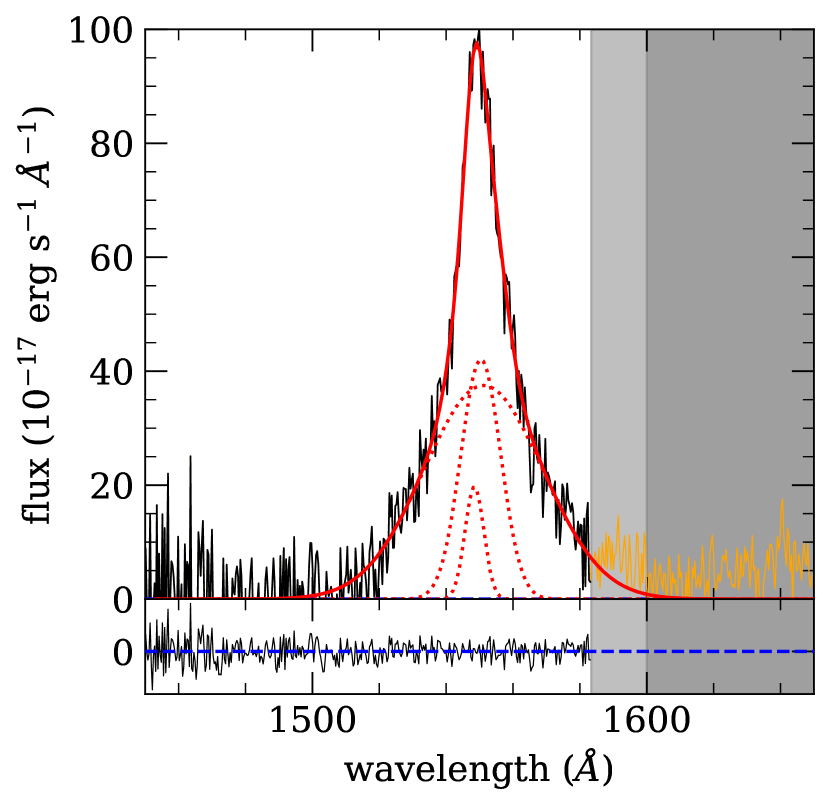
Figure 1: Example of the fitting procedure (GB6J162030+490149). The top panel represents the rest-frame continuum-subtracted spectrum. The mask applied is represented with the grey shaded area and in orange is shown the excluded part of the spectrum. The best-fitting model for the CIV line is represented with the solid red line, while the single gaussian components are depicted with the dotted red line. The bottom panel shows the residuals.

3.1 Spectral analysis

The procedure used to isolate and analyze the CIV emission line follows that described in Denney et al. (2016). The observed spectra are firstly corrected for Galactic extinction (Fitzpatrick, 1999). The redshift of the source is spectroscopically determined. We then bring the spectrum to the source rest-frame and linearly fit the continuum around the CIV emission line, using default windows of 1435–1465Å and 1690–1710Å (Denney et al., 2016). When the data within these boundaries are affected by spurious features or fall at the edge of the spectrum, other intervals are manually selected to estimate the continuum around the emission line. In many cases it was necessary to mask one or more regions containing spurious features, such as the emission often observed between CIV and HeII$\lambda$1640 (which requires a default mask between 1600Å and 1680Å, as in Denney et al., 2016), telluric absorptions, sky line residuals and cosmic rays. The fitting of the CIV line is performed with a multi-gaussians model (1, 2 or 3 depending on the spectrum and the data quality). To better illustrate the method, we report in Fig. 1 an example of the spectra preparation.
The fit parameters uncertainties are calculated using a Monte Carlo approach. For each object we create $N$ independent spectra based on the observed spectrum with a gaussian-distributed noise added. The noise is derived from the inverse variance vector when available, or from the RMS calculated in the continuum-subtracted spectrum around the line, when the vector was not present. For each mock spectrum the parameters are then estimated. After one thousand iterations, the standard deviation for each parameter is calculated and assumed as its uncertainty.
The best-fitting parameters with their uncertainties are reported in Table 2 . In particular, we show the best-fitting parameters of the z$>$4 sources while the values for the entire sample are reported in the Appendix.

3.2 Eddington Ratio

Another important parameter related to the mass of the central BH is the Eddington ratio i.e. the ratio between the bolometric luminosity and the Eddington luminosity:

$$\lambda_{edd}=L_{\text{bol}}/L_{\text{Edd}}$$ (8)

where $L_{\text{Edd}}=1.26\cdot 10^{38}M/M_{\sun}$ erg s^-1 and the bolometric luminosity is the total energy produced by the AGN per unit of time integrated on all the wavelengths. This parameter can be estimated using a bolometric correction (K${}_{\text{bol}}$) that allows the calculation of the bolometric luminosity starting from a monochromatic luminosity at a given wavelength (L${}_{\text{bol}}$=K${}_{\text{bol}}\cdot\lambda$L_λ). Here, we use an average K${}_{\text{bol}}$ derived from Shen et al. (2020): K${}_{\text{bol}}$($1450$Å)=4.68, which can be translated at $1350$Å using the average spectral index, resulting in K${}_{\text{bol}}$($1350$Å)$\approx 4.5$. The resulting values of Eddington ratios of the z$>$4 objects are reported in Table 2 while those of the entire sample appear in the Appendix.

3.3 Potential issues

Besides the statistical errors and the intrinsic scatter of the VP06 relations, the masses derived via the SE method are potentially affected by some (possible) systematics. We briefly discuss here the most important ones trying to establish their actual relevance on the sample considered in this work. At the end of the section we will present an independent measure of the masses showing that these biases, if present, should have a modest impact on our results (also considering the large statistical uncertainties). The main potential biases that may affect our SE-derived masses are:

• Orientation - Blazars are face-on RL AGNs. This means that we are likely observing these objects within $\sim 10^{\circ}$ from the jet direction (e.g. Savolainen et al., 2010; Ajello et al., 2012). It has been suggested (e.g. Decarli et al., 2008, 2010) that the typical BLR may have a disc-like structure and that the observed line widths are therefore significantly dependent on the particular orientation of the source since we only measure the projected component of the dispersion velocity. Therefore, in a nearly face-on source, the line width could be significantly lower than the edge-on case even if the mass of the central SMBH is the same. For a sample of randomly distributed AGNs, this effect will increase the scatter of the derived masses. In a sample of AGNs with a specific orientation, like blazars, the masses could be systematically biased.
  The SE relations (Eqs 6 and 7) are calibrated on several low-redshift quasars, for which we expect a random orientation (from 0 to $\sim 45$ degrees, by definition of type-I AGN). The SE relations are therefore strictly correct for a mean spatial angle, probably close to $\sim 30^{\circ}$. For sources observed at lower/larger angles, the derived mass is expected to be under/over estimated, respectively. However it is not clear if all the BELs are affected by orientation. This kind of bias has been actually measured by Runnoe et al. (2014) for masses calculated using H$\beta$ but it has not been found for CIV-based masses. A similar result has been achieved by Fine et al. (2011) using a sample of RL AGNs, finding no significant correlation between the CIV line width and the BLR orientation. The proposed explanation is that the highly ionized CIV line is probably produced in a different (more isotropic) region of the BLR. Therefore, we expect that the viewing angle is not a relevant issue in our estimate. However, as discussed in the next section (see 3.4), we have assessed this possible systematic using a completely independent method.
  

• Jet contamination and disk anisotropies - These potential issues are connected, again, with the orientation. Firstly, the luminosity of a relativistic jet observed at small angles is significantly amplified by the relativistic beaming (Urry & Padovani, 1995). In principle, this emission could contaminate the continuum emitted by the accretion disk. Therefore, a continuum-luminosity based relationship, like the one we are using (Eqs. 6 and 7), may lead to a mass overestimate (e.g. Decarli et al., 2010). Secondly, the continuum luminosity is known to be produced by a geometrically thin and optically thick disc-like structure, which means that the observed luminosity is higher when viewed face-on (Calderone et al., 2013). This effect could also lead to overestimate the mass, since the SE relations are calibrated on the average orientation of type-I AGNs, while we are applying them to sources observed face-on. In order to evaluate the impact of these potential bias on the SE masses, we have compared the CIV line luminosities (which are not affected by disc-inclination effects) against the continuum luminosities at 1350Å (which could be affected by the beaming). We then compared this relation with a similar one derived by Shen & Liu (2012) from a large sample of radio-quiet AGNs for which the beaming is not present and that are expected to be observed, on average, at larger angles compared to blazars. If the viewing angle plays a significant role in the observed continuum luminosity, we should observe a systematic shift of this relation with respect to the one by Shen & Liu (2012). Nevertheless, comparing the luminosities of the objects in our sample with those estimated in Shen et al. (2011) we find no evidence of a significant contamination (see Fig. 2). In particular, we can quantify the possible offset by considering the ratio $R=Log(L_{1350}/L_{CIV})$ in both the randomly aligned sample and in our sample. The two values ($R_{\text{Shen}}=1.62\pm 0.28$ and $R_{\text{blazar}}=1.61\pm 0.25$) are fully consistent.
  

  

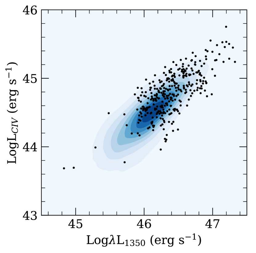
  Figure 2: Continuum luminosity versus CIV line luminosity. The plot represents the relation between the continuum luminosities estimated at 1350Å and the integrated line luminosities of the CIV, in our sample (black dots). As reference, we use the luminosities estimated in Shen et al. (2011) using a sample of randomly oriented AGNs (represented here with the blue confidence regions, in 10% increments). There is no evidence of any contamination from the jet, which would result in a systematic offset of the points with respect to the Shen et al. (2011) sample.

• Issues on the CIV line as a virial indicator - The SE method is based on the assumption that the line width arises from virial motions. However, as mentioned above, CIV BELs are affected by a blueshift, although this effect seems to be less relevant in RL AGNs (Richards et al. 2011). Due to the high ionization energy, CIV$\lambda$1549 is likely to be produced in the innermost part of the BLR, as confirmed by reverberation mapping observations of the CIV time-lag (Sun et al., 2018), and this effect may imply the presence of a non virialized component of the BLR. Indeed, the radiation pressure from the accretion disc may affect the regular trajectory of the gas, with a net radial radiation flow that modifies the emission line profiles (Murray & Chiang, 1997; Leighly, 2004; Denney, 2012). There have been many efforts to improve SE mass estimates from CIV (Denney, 2012; Runnoe et al., 2014; Mejía-Restrepo et al., 2016; Coatman et al., 2016). Nevertheless, Denney et al. (2013) found that the second moment of the line ($\sigma_{l}$) is only marginally affected by blueshift and that the masses derived through this quantity are less scattered with respect to the masses derived from H$\beta$ (provided that the S/N of the spectrum is high enough, namely S/N$\gtrsim$10 around 1450Å). For this reason, we decided to use the $\sigma_{l}$ to quantify the line widths of our sample. To allow a direct comparison with the literature, however, we also compute and report in Table 2 and in the Appendix the values of masses obtained using the (more common) relations based on the FWHM.

3.4 Testing the SE masses

Even if the potential issues described in the previous sections are not expected to have a significant impact on our analysis, we decided to verify the presence of any possible bias on the calculated masses. To this end, we use an independent technique based on the accretion disc emission (e.g. see Calderone et al., 2013 for a detailed description of the method). This technique assumes that the optical/UV continuum emission of the AGN is produced by an optically thick, geometrically thin accretion disc (AD) that emits according to the Shakura & Sunyaev (1973, SS73) model. With these assumptions it is possible to derive the values of M${}_{\text{BH}}$ and of the accretion rate, that are free parameters of the SS73 model, simply by fitting the optical/UV data points. In spite of its simplicity, the AD method is not routinely used to derive the SMBH masses since it requires a good data coverage, in particular around the critical region where the disc emission peaks (i.e. the rest-frame UV region). For this reason, this method is typically applied to high-z objects (z$>$3–4) for which the rest-frame UV region of the spectrum is relatively well sampled by the photometric points in the visible range. However, even in high-z sources the application of this technique could be problematic since the peak of the disc emission may fall at wavelengths bluer than the Ly$\alpha\lambda 1215$ where the effect of the neutral hydrogen absorption is very important, making the photometric points not usable. This happens, in particular, in sources hosting the least massive SMBHs ($<$10⁸ M_☉).
With the main goal of testing the SE masses, we decided to apply the AD method to the high-z (z$\geq$4) objects in the CLASS sample, for which the UV spectral range is relatively well sampled. The typical photometric coverage available for CLASS high-z sources is limited to the few data points from PS1 not affected by the neutral hydrogen absorption and to the observed spectrum. MID-IR points from the Wide-field Infrared Survey Explorer (WISE, Wright et al., 2010) cannot be used as they may be contaminated by the jet emission.
As a consequence of this limited data set, the resulting masses are poorly constrained, with typical uncertainties of $\sim$0.3–0.6 dex, that are significantly larger than the statistical error on the masses derived from SE method ($\sim$0.05 dex) and comparable or even larger than the intrinsic error related to the SE method ($\sim$0.4 dex). In spite of these large uncertainties, the AD method can be still used to search for possible systematics in the SE masses.

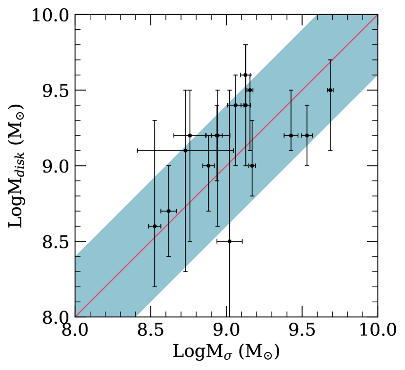
Figure 3: Comparison of the SMBH masses (z$\geq$4) derived using the SE and the AD method. The red solid line is the 1:1 relation; in cyan, the region corresponding to the maximum intrinsic scatter of the VP06 relations (0.4 dex). No evident bias in the mass estimate can be revealed using this independent method.

In Fig 3 we show the comparison between the SE masses of the C19 sample (based on Eq. 7) and the AD masses.
Given the large uncertainties of the AD masses, the two values are overall in good agreement (Log$({M}_{\text{disk}}/{M}_{\text{SE}})=0.1\pm 0.3$).
In conclusion, the masses derived with the SE method, although very uncertain, do not reveal systematic discrepancies when compared to the AD masses. This confirms that the potential biases, discussed in the previous section, if present, do not affect significantly the final results. We therefore consider the SE masses as our best estimates and we use them in the rest of the paper.

4 Space density evolution of $\geq 10^{9}$M_☉ SMBHs hosted by RL AGNs

	Starting sample	With spectra	$M_{\text{SMBH}}\geq 10^{9}$M☉
N sources	380	352	243

Table 3: Number of sources selected. The number of sources, between z=1.5 and z=5.5, in the progressively stringent sets considered. Respectively, the starting sample (Eqs. 1, 2 and $|b\arcsec|\geq 20$) composed by 361 objects with 1.5$\leq$z$<$4 plus the C19 sample (19 sources with 4$\leq$z$<$5.5); the objects with an available spectrum; the objects with a $M_{\text{SMBH}}\geq 10^{9}$M_☉ (considering the line dispersion relation, Eq. 7).

An important test to assess the role of the relativistic jets in the evolution of the SMBHs across cosmic time is to compare the relative abundance of RL AGNs with respect to the total AGN population at different redshifts. The RL fraction in the local Universe has been the subject of several publications in the last years. The commonly accepted value was assessed to be about $\sim 10\%$ (e.g. Fanti et al., 1977; Condon et al., 1980; Smith & Wright, 1980; Sramek & Weedman, 1980; Hooper et al., 1995; Ivezić et al., 2002; Volonteri et al., 2011) although some more recent works have found that the RL fraction could be as high as 20–30% (e.g. Kellermann et al., 1989; della Ceca et al., 1994; Best et al., 2005; Jiang et al., 2007; Kellermann et al., 2016).
However, estimating this ratio at larger redshift is not as straightforward (e.g. Stern et al., 2000; Bañados et al., 2015; Yang et al., 2016; Liu et al., 2021). As already discussed, part of the radio emission, i.e. the one produced by the jet, is highly anisotropic because of the relativistic beaming that strongly boosts the emission along the jet direction. This problem is particularly important at high redshifts where we typically observe the high frequency (rest-frame) emission which is usually dominated by the jet while the isotropic component (from the radio lobes) is severely attenuated due to the steepness of the spectrum. In addition, the extended emission is more difficult to detect compared to the point-like core, especially with fluxes close to the survey sensitivities. Finally, the extended emission of RL AGNs is also expected to be significantly damped at high redshift due to the increased density of the CMB photons that interact and cool the relativistic electrons in the radio lobes (see e.g. Ghisellini et al., 2014a). All these potential issues make it difficult to assess whether the optically selected high-z AGNs currently not detected in the radio band are truly radio-quiet sources or simply misaligned jetted AGNs. Using blazars to trace the RL AGNs population, instead, we are not directly affected by these problems and, therefore, we can provide a reliable estimate of the true fraction of RL AGNs at all redshifts.

As discussed in Section 2, our sample is complete for radio powers larger than P${}_{5\text{GHz}}\gtrsim 10^{27}$ W Hz^-1. Considering that we expect the radio luminosity in blazars to be boosted by 2 or 3 orders of magnitude , this means that we are able to sample the population of RL AGNs down to an intrinsic radio power of P${}_{5\text{GHz}}\sim 10^{24}$–$10^{25}$ W Hz^-1 which is close to the typical threshold that divides radio-loud from radio-quiet AGNs (e.g. Kellermann et al., 2016; Padovani, 2017). Considering the deboosted radio flux, our sample is sensitive to an intrinsic radio-loudness. This means that we should be sensitive to the bulk of the RL AGNs population up to z$\sim$5.5.

In principle, the presence of an optical limit (mag=21 for the z$\geq$4 sample) may prevent the selection of the least (optical) luminous sources ($\lambda$L${}_{\lambda}(1350\text{\AA})<10^{46}$erg s^-1). As previously discussed, however, we are focusing on the objects hosting the largest SMBH masses (M$\geq 10^{9}$ M_☉, i.e. 243 sources, see Tab. 3). The limit on the optical luminosity can be translated into a limit on the bolometric luminosity:

$$L_{\text{bol}}=K_{\text{bol}}(1350\text{\AA})\cdot\nu L_{\nu}(1350\text{\AA})\simeq 5\cdot 10^{46}\text{ erg s}^{-1}$$ (9)

For SMBH masses between 10⁹ and 10¹⁰ M_☉, this limit implies that we are sensitive down to Eddington ratios of $\sim$0.1–0.2, i.e. again, to the bulk of the population of AGNs with quasar-like spectra (Shen et al., 2011). In summary, with the CLASS blazars we are able to evaluate the true space density of RL AGNs hosting the most massive SMBHs ($M\geq 10^{9}$M_☉) in the 1.5–5.5 redshift range.

First, for each source we calculate the comoving volume within which it could have been observed:

$$V_{\text{eff}}=\frac{A}{4\pi}V$$ (10)

where A is the sky coverage area in steradians of the two sub-samples, i.e. 1.272$\pi$ (or $13120\text{\leavevmode\nobreak\ deg}^{2}$) above z=4, 1.038$\pi$ (or $10700\text{\leavevmode\nobreak\ deg}^{2}$) under z=4. $V$ is the comoving volume between $z_{1}$ and $z_{2}$. Please note that in this case it is not necessary to apply the method suggested in Avni & Bahcall (1980), since in our luminosity-limited sample each object is always detectable up to z$\sim$5.5. The blazar space density in each bin (z₁,z₂) is therefore calculated as:

$$n_{\text{blazar}}=\frac{C_{\text{spect}}\cdot C_{\text{id}}\cdot N}{V_{\text{eff}}}$$ (11)

The sources of uncertainty in the blazars space density calculation are the coefficients (C${}_{\text{id}}$ and C${}_{\text{spect}}$, distributed with a binomial pdf, see Section 2) and the Poisson uncertainty on the number of objects above the considered mass threshold (M$\geq$10⁹M_☉) which, in turns, depends on the uncertainty on the SE masses (Gauss distribution with standard deviation $\sigma=0.3M_{\sun}$, see Section 3). In order to evaluate the impact of these sources of uncertainties we performed a Monte Carlo simulation with 10⁵ iterations.

Finally, we can consider the blazars space density inferred from the only $z\sim 6$ blazar known to date ($0.0055\begin{subarray}{c}+0.0125\\ -0.0046\end{subarray}$ Gpc^-3, Belladitta et al., 2020 and Belladitta et al. submitted).

In order to evaluate the space density of all RL AGNs hosting a SMBH with $M_{\text{BH}}\geq 10^{9}$M_☉ ($n_{\text{jet}}$), as mentioned in Sec. 1, we use a simple geometrical argument:

$$n_{\text{jet}}=2\Gamma^{2}n_{\text{blazar}}$$ (12)

In this paper we assume a mean $\Gamma=10$, therefore 1 blazar every $\sim$200 RLs. The results are reported in Tab. 4 and in Fig. 4.

z bin	N${}_{\text{bl}}$	Log$n_{\text{bl}}$		Log$n_{\text{jet}}$
				$\Gamma$
			5	10	15
$1.50-1.75$	26	0.04$\begin{subarray}{c}+0.10\\ -0.11\end{subarray}$	1.74	2.34	2.69
$1.75-2.00$	26	0.00$\begin{subarray}{c}+0.10\\ -0.11\end{subarray}$	1.70	2.31	2.66
$2.00-2.25$	37	0.16$\begin{subarray}{c}+0.08\\ -0.09\end{subarray}$	1.86	2.46	2.82
$2.25-2.50$	30	0.08$\begin{subarray}{c}+0.09\\ -0.10\end{subarray}$	1.78	2.38	2.73
$2.50-2.75$	34	0.12$\begin{subarray}{c}+0.08\\ -0.09\end{subarray}$	1.82	2.42	2.78
$2.75-3.00$	31	0.11$\begin{subarray}{c}+0.08\\ -0.09\end{subarray}$	1.81	2.41	2.76
$3.00-3.50$	33	-0.12$\begin{subarray}{c}+0.08\\ -0.09\end{subarray}$	1.57	2.18	2.53
$3.50-4.00$	14	-0.43$\begin{subarray}{c}+0.12\\ -0.13\end{subarray}$	1.27	1.87	2.22
$4.00-4.50$	8	-0.94$\begin{subarray}{c}+0.15\\ -0.24\end{subarray}$	0.76	1.36	1.72
$4.50-5.00$	2	-1.52$\begin{subarray}{c}+0.37\\ -0.45\end{subarray}$	0.18	0.78	1.14
$5.00-5.50$	2	-1.49$\begin{subarray}{c}+0.37\\ -0.45\end{subarray}$	0.21	0.81	1.16

Table 4: Space density of the most massive ($\geq 10^{9}M_{\sun}$) blazars in our sample. Column 1: redshift interval; column 2: the number of blazars, within the sample, with a mass $M\geq 10^{9}$M_☉ in each bin of redshifts in the covered sky area; column 3: logarithmic space density of blazars with $M\geq 10^{9}$M_☉ (measured in Gpc^-3); column 4, 5 and 6: logarithmic space density of jetted AGNs, inferred assuming three representative Lorentz bulk factors, i.e. $\Gamma=[5,10,15]$ (measured in Gpc^-3). The statistical uncertainties on the logarithmic jetted AGNs densities are the same as for the logarithmic blazar densities.

5 Discussion

So far we have derived the space density of blazars hosting the most massive SMBHs ($\geq 10^{9}$M_☉) at 1.5$\leq$z$\leq$5.5. Using a geometrical argument, assuming a viewing angle $\theta\sim 1/\Gamma$ and a typical Lorentz bulk factor $\Gamma=10$, we have inferred the space density of all the jetted AGNs powered by the most massive SMBHs, in the considered redshift interval. We want to stress that this estimate is by definition unaffected by the torus dust extinction, therefore we are including in our result both the type-I and the type-II AGNs, at least in the case that the obscuration is only due to a molecular torus. It is known that jetted AGNs represent a minority of the total population, and several works have tried to estimate the relative abundance of these objects. These estimates converge to 10–30% in the local Universe (e.g. Fanti et al., 1977; Condon et al., 1980; Smith & Wright, 1980; Sramek & Weedman, 1980; Hooper et al., 1995; Ivezić et al., 2002; Kellermann et al., 1989; Best et al., 2005; Jiang et al., 2007; Volonteri et al., 2011; Kellermann et al., 2016). However, it is still unclear if the jetted fraction have changed with cosmic time, especially at high-z, due to the lack of consistency in the samples at different redshifts and the intrinsic difficulty of observing partially or completely obscured jetted AGNs.
In order to compare the most massive SMBHs hosted in jetted AGNs with those hosted by the total AGN population, we would need complete samples containing the values of SMBH masses for each source, as in our sample of blazars. Alternatively, it is possible to use the quasar luminosity function (QLF) and integrate it above a certain effective luminosity, considering that SMBH mass and bolometric luminosity are tightly related. In particular, we use the most recent QLF derived in Shen et al. (2020) . This QLF is corrected for intrinsic absorption assuming the neutral hydrogen column distribution suggested in Ueda et al. (2014), and a redshift-dependent dust-to-gas ratio (Ma et al., 2015). Therefore, without further corrections, we can directly compare our results with this QLF.
In particular we integrate the QLF with a minimum luminosity:

$$n_{\text{AGN}}(z)=\int_{L^{\text{eff}}_{min}}^{\infty}n_{\text{AGN}}(z,L)dL$$ (13)

Where $n_{\text{AGN}}(z)$ is the number density of AGNs hosting the most massive BHs ($\geq 10^{9}$M_☉); considering the objects with M$\geq 10^{9}$M_☉ in our sample, we can define L${}^{\text{eff}}_{min}$ as the minimum luminosity to obtain the same number of objects within our full sample of 380 objects, regardless of M${}_{\text{BH}}$, with L${}_{\text{bol}}\geq$L${}^{\text{eff}}_{min}$. We find L${}^{\text{eff}}_{min}=8.4\cdot 10^{46}$ erg s^-1. Thus, we can integrate the QLF without assuming a specific Eddington ratio distribution.

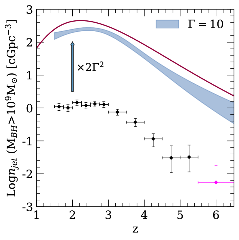
Figure 4: Comoving space density of different types of AGNs hosting black holes with $M\geq 10^{9}$M_☉ as a function of redshift. The black dots represent the space density of SMBHs with $M\geq 10^{9}$M_☉ hosted by FSRQs, estimated in this work. The magenta dot represents the blazars space density inferred from the only blazar known at z>6 (Belladitta et al., 2020), which is in good agreement with the extrapolation of our points. The uncertainties on the densities are estimated using a Monte Carlo simulation (see text). The blue band indicates the space density of all RL AGNs, independently of orientation (i.e. including absorbed sources), as estimated from the blazar population. It is derived by fitting the black points and then scaling up the normalization by a factor $2\Gamma^{2}$, assuming a mean Lorentz factor $\Gamma=10$. The delimited area represents 1$\sigma$ confidence intervals, calculated using a Monte Carlo method. The dark red solid line is derived from the most recent QLF (Shen et al., 2020) which estimates the space density of both jetted and non-jetted AGNs, up to z=6.5. In particular, the QLF is integrated with $L^{\text{eff}}_{\text{min}}\geq 8.4\cdot 10^{46}$ erg s^-1, in order to represent only quasars similar to the bulk of our sample (see text).

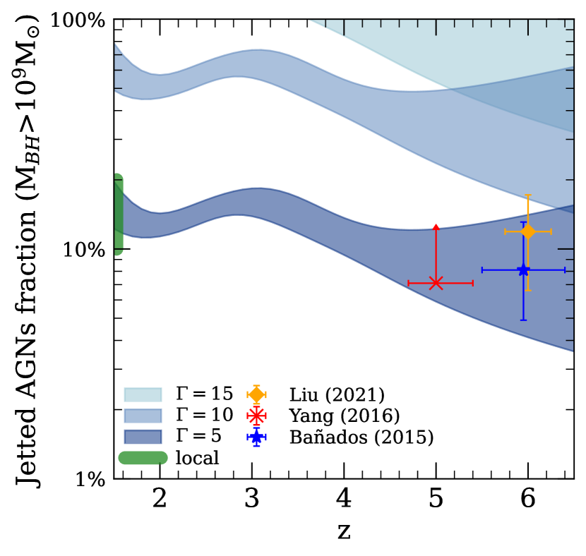
Figure 5: Fraction of jetted AGNs hosting the most massive SMBHs ($\geq 10^{9}$M_☉) as a function of redshift. We report here three different estimates assuming three values of the Lorentz factor: $\Gamma=[5,10,15]$. The uncertainties are estimated using a Monte Carlo method and are the same as in Fig. 4. Coloured dots represent previous estimates found in the literature (see the inset).

The integrated QLF shows a luminosity dependent evolution, with a maximum density occurring at z=2.2 using the aforementioned lower luminosity (see Fig. 4, dark red line).
The first fact that emerges from the comparison is that the space density evolution of jetted AGNs here calculated is qualitatively similar to that observed in the total AGN population. This is in contrast with previous results that found a much more rapid evolution in X-ray selected blazars with similar masses, culminating at $z\sim 4$ (Ajello et al., 2009). One possible explanation for this discrepancy is that the X-ray-to-radio luminosity ratio of the jet emission strongly increases with redshift, as actually observed by several authors (e.g. Zhu et al., 2019 and Ighina et al., 2019). This increase is naturally expected if we consider the Inverse Compton interaction between the photons from the Cosmic Microwave Background (CMB) and the electrons present in the relativistic jets. This interaction is expected to produce a progressive enhancement of the X-ray emission in high-z blazars, since the CMB photon density increases as $(1+z)^{4}$. Using this model, Ighina et al. (2021) found that the space densities of radio-selected (Mao et al., 2017) and X-ray-selected (Ajello et al., 2009) blazars can be nicely reconciled. In this picture, the apparent increase of the space density of X-ray selected blazars at high redshift is only a consequence of the progressive enhancement of their typical X-ray luminosity.

In spite of the similar global behaviour of the two distributions in Fig. 4, we can notice some possible differences. First, the space density peak of the most massive SMBHs hosted by jetted AGNs seems to occur at slightly higher redshift (z${}_{\text{peak}}\sim 3$) when compared to that of the entire AGNs population (z${}_{\text{peak}}\sim 2.2$). In order to better quantify this difference we can fit the jetted AGNs space density (obtained using Eq. 12 with $\Gamma=10$), as a function of z, with a simple double power law model:

$$n(z)=\frac{2n_{0}}{\left(\frac{1+z}{1+z_{0}}\right)^{\gamma_{1}}+\left(\frac{1+z}{1+z_{0}}\right)^{\gamma_{2}}}$$ (14)

With $\gamma_{1}$ and $\gamma_{2}$ representing the two slopes, $\rho_{0}$ is a normalization parameter and $z_{0}$ represents the break point. The uncertainties are calculated using a Monte Carlo simulation and are given at 68% confidence level. The best fit value of $z_{0}$ is $2.98\pm 0.27$.
This is not consistent with the total AGN population density peak. This in turn seems to suggest that the comoving space density of the most massive SMBHs hosted by jetted AGNs reach the maximum value about $\sim$800 Myr before those hosted by the total AGN population. Another possible difference between the two curves of Fig. 4 is the flatter slope at redshifts below the peak observed in the RL AGNs compared to the total population. This is, however, an uncertain result since we are sampling only a relatively narrow range of redshifts below z<2. We want to stress here that the evolutionary shape of the jetted space density is independent of the choice of the Lorentz bulk factor, which is highly uncertain and can only change the overall normalization of the global evolutionary pattern (unless the average value of $\Gamma$ changes across the considered range of redshifts).

Finally, we can evaluate the evolution of the fraction of the jetted AGNs hosting the most massive SMBHs with respect to the total population. In Fig. 5 we report the percentage fraction of the jetted AGNs estimated in our work, using three representative values of $\Gamma=[5,10,15]$. Clearly, given the uncertainty on the value of $\Gamma$, we cannot tightly constrain the absolute value of RL AGNs. However, assuming that the average value of $\Gamma$ does not change with z, we can establish whether the fraction of jetted AGNs hosting a massive SMBH has changed between z$\sim$1 up to z$\sim$6. Fig. 5 seems to suggest a progressive decrease of this fraction by a factor $\sim$2, going from z$\sim$1 to z$\sim$5, independently to the assumed average value of $\Gamma$. This is in line with what was found by other authors (e.g. Jiang et al., 2007; Kratzer, 2014).

In addition, we can compare our result with some independent estimates of the RL fraction published in the literature. In Fig. 5 we report the high-redshift estimates derived by directly counting the known RL AGNs (not necessarily blazars). We consider here only the estimates based on samples with similar optical luminosity limit, namely: $-29<M_{1450}<-26.8$ (Yang et al., 2016); PS1 $i<22.6$, at z$\sim$6 (Bañados et al., 2015); $M_{1450}<-25.5$ (Liu et al., 2021, luminous sample) and with similar deboosted radio luminosity limit $f_{\text{1.4GHz}}>1$mJy. We want to stress that this method, as mentioned above, could be affected by numerous biases that can be avoided focusing on blazars instead. However, considering all the uncertainties, our results are consistent with the estimates from the literature assuming a Lorentz bulk factor between $\approx$6 and 8.
We can also compare our results with the observed local fraction of RL AGNs. To this end we want to consider an estimate based on a sample with similar properties, since some recent works seem to suggest that the RL fraction may depend on the mass and the luminosity of the SMBH (e.g. Cirasuolo et al., 2003; Jiang et al., 2007; Rafter et al., 2009; Yang et al., 2016). Jiang et al. (2007), in particular, gives an independent estimate of the RL fraction as a function of both luminosity and redshifts. Focusing on $z\sim 1.5$ we find that the local RL fraction is estimated to be 10%–20%, consistent with our low-redshift value assuming again a $\Gamma\approx 5$.

6 Conclusion

We have assembled a complete and well-defined sample of 380 blazars (FSRQs) with a similar range of optical/radio luminosities ($\lambda$L${}_{1350}\gtrsim 10^{46}$ erg s^-1, P${}_{5\text{GHz}}\gtrsim 10^{27}$ W Hz^-1) hosting SMBHs with masses $\geq 10^{9}$M_☉, across a wide redshift interval (1.5$\leq$z$\leq$5.5). We have used this statistically complete sample to infer the evolutionary path of all the jetted AGNs with similar properties, and we have compared the result with the total AGN population, using the most recent QLF available to date (Shen et al., 2020). The findings can be summarized as follow:

• Differently from the overall AGNs population, the jetted AGNs space density shows a peak at a slightly higher redshift ($z\sim 3$ as opposed to $z\sim 2.2$) but not so extreme as the value previously inferred using X-ray selected blazars ($z\sim 4$).

• There is a marginal evidence of a flat density evolution in the jetted AGNs population at z<3 whereas the overall population density strongly decreases.

• The jetted AGNs fraction seems to decrease by a factor of 2 going from $z\sim 1$ to $z\sim 5$.

• Assuming a mean Lorentz bulk factor $\Gamma\approx 5$ the jetted AGNs fraction is overall consistent with the values estimated in the literature in the local Universe (10–20%) and at high redshifts.

The possible differences in the cosmological evolution of SMBHs hosted by jetted and non-jetted AGNs should be investigated more carefully using larger samples of blazars. In particular, in order to establish more accurately the peak position we need to improve the statistics at z$\sim$2-3. At the same time, the investigation of any difference in the slope at z>2 between the two populations requires to better sample the very high redshift end of the curve (z>5), where only few blazars have been discovered to date. Sampling this very high-z part of the blazar population is also critical to fully understand the origin of the difference observed between radio and X-ray selected blazars. Indeed, our results seem to rule out the presence of a peak at z$\geq$4, previously suggested by X-ray selected surveys. As already explained, this discrepancy could be connected to a progressive increase of the X-ray-to-radio luminosity ratio with redshift, possibly caused by the interaction of jet with the photons from the CMB (Ighina et al., 2021). To further test this (and other) hypotheses it is fundamental to significantly increase the statistics at redshift above 5.5 where the effect of CMB is expected to be more and more relevant and where only one blazar has been discovered to date.

Creating sizable samples of blazars at such high redshifts is very challenging given the particular scarcity of these sources. A big leap forward is expected in the next years thanks to the new wide area surveys, covering most of the sky, that will be carried out by the new generation of radio (Square Kilometre Array, SKA, and its precursors), X-ray (extended Röntgen Survey with an Imaging Telescope Array, eROSITA and Athena) and optical/IR (e.g. the Vera C. Rubin Observatory and Euclid) telescopes. The joint use of data covering such a large portion of the sky and of the electromagnetic spectrum has been proven to be crucial to efficiently select high-z blazars. In addition, given the extreme faintness of the expected counterparts, a fundamental role will be also played by the incoming large optical/IR telescopes, like Extremely Large Telescope, ELT, and James Webb Space Telescope, JWST, that will guarantee a reliable spectroscopic follow-up. We are confident that in the near future the same kind of study discussed here will be feasible up to z$\sim$7-8 and for less massive objects allowing us to better constrain the global evolution of SMBHs in jetted AGNs and to understand the actual role of the relativistic jets in the global picture.

Data Availability

The data underlying this article are available in the article and in its online supplementary material.

Appendix A Full sample data

Table 5: Properties of the FSRQs in our sample. column 1: source name; column 2: redshift; column 3: total extinction in the V-band; column 4: magnitude in the r-filter ; column 5: radio flux density measured at 5GHz; columns 6 and 7: CIV line dispersion and FWHM; column 8: continuum luminosity at 1350Å  column 9: CIV$\lambda$1549 line luminosity; column 10: bolometric luminosity, calculated assuming a bolometric correction K${}_{\text{bol}}(1350\text{\AA})=4.5$; columns 11 and 12: SMBH mass, estimated using the VP06 relations (see text); columns 13 and 14: Eddington ratios calculated using the masses derived from the line dispersion and the FWHM, respectively.

name	z	AV	r-mag	S${}_{\text{5GHz}}$	$\sigma_{l}$	FWHM	Log$\lambda$L1350	LogLCIV	LogL${}_{\text{bol}}$	LogMσ	LogM${}_{\text{FWHM}}$	Log$\lambda_{\text{Edd}}$	Log$\lambda_{\text{Edd}}$
				(mJy)	(km s-1)	(km s-1)	(erg s-1)	(erg s-1)	(erg s-1)	(M☉)	(M☉)	[$\sigma_{l}$]	[FWHM]
GB6J000026+030706	2.35	0.148	18.74	91	$3091\pm 161$	$5613\pm 373$	$46.515\pm 0.005$	$44.487\pm 0.011$	$47.168\pm 0.005$	$9.04\pm 0.04$	$9.49\pm 0.06$	$0.02\pm 0.04$	$-0.42\pm 0.06$
GB6J000345+160536	2.31	0.198	19.49	109	$4802\pm 539$	$4838\pm 291$	$46.383\pm 0.006$	$44.481\pm 0.012$	$47.036\pm 0.006$	$9.36\pm 0.09$	$9.29\pm 0.05$	$-0.42\pm 0.09$	$-0.36\pm 0.05$
GB6J000519+052349	1.90	0.212	16.23	303	-	-	-	-	-	-	-	-	-
GB6J000649+242232	1.68	0.276	18.79	189	$4390\pm 1472$	$4064\pm 465$	$46.260\pm 0.005$	$44.885\pm 0.667$	$46.913\pm 0.005$	$9.21\pm 0.23$	$9.08\pm 0.11$	$-0.40\pm 0.23$	$-0.26\pm 0.12$
GB6J000917+062549	2.69	0.292	19.42	156	$3064\pm 95$	$4451\pm 261$	$46.323\pm 0.005$	$44.104\pm 0.014$	$46.977\pm 0.005$	$8.93\pm 0.03$	$9.19\pm 0.05$	$-0.06\pm 0.03$	$-0.31\pm 0.05$
GB6J000942+151357	2.24	0.252	19.74	121	$3415\pm 508$	$3484\pm 389$	$45.746\pm 0.017$	$44.315\pm 0.014$	$46.399\pm 0.017$	$8.72\pm 0.09$	$8.67\pm 0.10$	$-0.42\pm 0.09$	$-0.37\pm 0.10$
GB6J001033+172437	1.60	0.196	16.70	989	-	-	-	-	-	-	-	-	-
GB6J001115+144608	4.96	0.242	19.62	31	$3310\pm 138$	$7548\pm 322$	$47.326\pm 0.004$	$45.240\pm 0.012$	$47.979\pm 0.004$	$9.53\pm 0.04$	$10.18\pm 0.04$	$0.35\pm 0.04$	$-0.30\pm 0.04$
GB6J001144+292820	2.63	0.225	19.24	107	$2308\pm 113$	$3097\pm 358$	$46.450\pm 0.008$	$44.554\pm 0.012$	$47.103\pm 0.008$	$8.76\pm 0.04$	$8.94\pm 0.10$	$0.25\pm 0.04$	$0.06\pm 0.10$
GB6J001154+083359	2.20	0.474	19.84	87	$3975\pm 119$	$4258\pm 405$	$45.819\pm 0.010$	$44.195\pm 0.013$	$46.472\pm 0.010$	$8.89\pm 0.03$	$8.88\pm 0.08$	$-0.52\pm 0.03$	$-0.51\pm 0.09$
GB6J001307+205335	3.53	0.199	17.80	41	-	-	-	-	-	-	-	-	-
GB6J001837+041532	2.70	0.137	19.78	142	$4693\pm 1118$	$3290\pm 431$	$45.911\pm 0.018$	$44.715\pm 0.025$	$46.564\pm 0.018$	$9.09\pm 0.17$	$8.71\pm 0.12$	$-0.62\pm 0.17$	$-0.24\pm 0.12$
GB6J002121+155127	3.70	0.209	19.64	35	$4796\pm 210$	$3677\pm 206$	$46.440\pm 0.011$	$44.945\pm 0.012$	$47.093\pm 0.011$	$9.38\pm 0.04$	$9.08\pm 0.05$	$-0.39\pm 0.04$	$-0.09\pm 0.05$
GB6J002903+050931	1.63	0.128	18.53	377	$4952\pm 398$	$5032\pm 301$	$45.958\pm 0.013$	$44.484\pm 0.012$	$46.611\pm 0.013$	$9.16\pm 0.07$	$9.10\pm 0.05$	$-0.65\pm 0.07$	$-0.59\pm 0.05$
GB6J003443+275423	2.96	0.256	18.39	587	$2907\pm 88$	$2903\pm 369$	$46.877\pm 0.004$	$45.214\pm 0.009$	$47.530\pm 0.004$	$9.18\pm 0.03$	$9.11\pm 0.12$	$0.25\pm 0.03$	$0.32\pm 0.12$
GB6J003544+143803	2.45	0.248	19.37	328	$7775\pm 682$	$3871\pm 301$	$46.273\pm 0.008$	$44.758\pm 0.014$	$46.926\pm 0.008$	$9.72\pm 0.08$	$9.04\pm 0.07$	$-0.89\pm 0.08$	$-0.21\pm 0.07$
GB6J003759+160629	3.34	0.203	20.60	77	$3789\pm 742$	$3677\pm 590$	$45.711\pm 0.036$	$44.474\pm 0.015$	$46.364\pm 0.036$	$8.79\pm 0.10$	$8.70\pm 0.14$	$-0.53\pm 0.10$	$-0.43\pm 0.15$
GB6J010037+334513	2.14	0.278	19.68	119	$3748\pm 68$	$6774\pm 360$	$45.865\pm 0.013$	$44.766\pm 0.006$	$46.518\pm 0.013$	$8.87\pm 0.02$	$9.31\pm 0.05$	$-0.45\pm 0.02$	$-0.89\pm 0.04$
GB6J010838+013516	2.10	0.126	18.09	4180	$4421\pm 544$	$3290\pm 539$	$46.772\pm 0.004$	$44.973\pm 0.015$	$47.426\pm 0.004$	$9.49\pm 0.08$	$9.16\pm 0.14$	$-0.17\pm 0.08$	$0.16\pm 0.14$
GB6J010838+140428	1.70	0.193	19.01	132	$3224\pm 81$	$2322\pm 227$	$46.287\pm 0.007$	$44.509\pm 0.009$	$46.941\pm 0.007$	$8.96\pm 0.02$	$8.60\pm 0.08$	$-0.12\pm 0.02$	$0.24\pm 0.09$
GB6J011114+171320	2.20	0.260	19.51	99	$5512\pm 863$	$3871\pm 372$	$46.216\pm 0.007$	$44.708\pm 0.015$	$46.869\pm 0.007$	$9.39\pm 0.12$	$9.01\pm 0.09$	$-0.62\pm 0.12$	$-0.24\pm 0.09$
GB6J011636+290406	3.28	0.302	18.69	68	$4129\pm 243$	$2710\pm 335$	$46.561\pm 0.009$	$45.097\pm 0.010$	$47.215\pm 0.009$	$9.32\pm 0.06$	$8.88\pm 0.11$	$-0.20\pm 0.05$	$0.23\pm 0.11$
GB6J012129+112702	2.49	0.206	17.23	194	$3201\pm 76$	$3290\pm 483$	$46.987\pm 0.004$	$44.767\pm 0.014$	$47.640\pm 0.004$	$9.32\pm 0.02$	$9.28\pm 0.14$	$0.22\pm 0.02$	$0.26\pm 0.14$
GB6J012202+030951	4.00	0.161	20.86	96	-	$5800\pm 2000$	$46.450\pm 0.070$	-	$47.103\pm 0.070$	-	$9.52\pm 0.39$	-	$-0.51\pm 0.39$
GB6J012238+250238	2.02	0.408	19.07	764	$3932\pm 460$	$5032\pm 485$	$46.028\pm 0.012$	$44.981\pm 0.012$	$46.681\pm 0.012$	$8.99\pm 0.09$	$9.14\pm 0.08$	$-0.41\pm 0.09$	$-0.56\pm 0.09$
GB6J012642+255902	2.36	0.458	18.13	1303	$3628\pm 48$	$3871\pm 560$	$46.839\pm 0.003$	$45.179\pm 0.012$	$47.492\pm 0.003$	$9.35\pm 0.01$	$9.34\pm 0.17$	$0.04\pm 0.01$	$0.05\pm 0.17$
GB6J012921+310303	3.56	0.265	19.48	74	$8055\pm 584$	$4838\pm 439$	$46.583\pm 0.009$	$44.853\pm 0.013$	$47.236\pm 0.009$	$9.91\pm 0.06$	$9.40\pm 0.08$	$-0.78\pm 0.06$	$-0.26\pm 0.08$
GB6J013942+175253	2.72	0.296	18.71	301	$4089\pm 258$	$3097\pm 263$	$46.574\pm 0.005$	$45.037\pm 0.009$	$47.227\pm 0.005$	$9.32\pm 0.05$	$9.01\pm 0.08$	$-0.19\pm 0.05$	$0.12\pm 0.08$
GB6J015235+335037	2.41	0.261	18.23	611	$3442\pm 47$	$6193\pm 183$	$46.733\pm 0.005$	$44.819\pm 0.008$	$47.386\pm 0.005$	$9.25\pm 0.01$	$9.69\pm 0.03$	$0.03\pm 0.01$	$-0.41\pm 0.03$
GB6J015855+130705	1.89	0.324	18.91	272	$3688\pm 246$	$4451\pm 300$	$46.358\pm 0.022$	$44.748\pm 0.011$	$47.011\pm 0.022$	$9.11\pm 0.06$	$9.21\pm 0.06$	$-0.20\pm 0.06$	$-0.30\pm 0.06$
GB6J015923+310648	2.25	0.263	18.35	190	$6628\pm 1129$	$3097\pm 1207$	$46.572\pm 0.005$	$45.030\pm 0.176$	$47.225\pm 0.005$	$9.74\pm 0.13$	$9.00\pm 0.21$	$-0.61\pm 0.13$	$0.12\pm 0.21$
GB6J020310+263246	3.35	0.387	19.58	77	$3819\pm 138$	$3097\pm 230$	$46.498\pm 0.008$	$45.127\pm 0.008$	$47.151\pm 0.008$	$9.22\pm 0.03$	$8.97\pm 0.06$	$-0.17\pm 0.03$	$0.09\pm 0.06$
GB6J020521+241624	2.45	0.424	19.28	243	$4293\pm 441$	$2516\pm 280$	$46.319\pm 0.005$	$44.847\pm 0.016$	$46.972\pm 0.005$	$9.22\pm 0.09$	$8.69\pm 0.10$	$-0.35\pm 0.09$	$0.18\pm 0.10$
GB6J021436+015702	3.28	0.170	19.48	103	$2762\pm 80$	$6387\pm 206$	$46.272\pm 0.016$	$44.407\pm 0.009$	$46.926\pm 0.016$	$8.82\pm 0.03$	$9.47\pm 0.03$	$0.01\pm 0.03$	$-0.65\pm 0.03$
GB6J021748+014451	1.72	0.173	16.18	1419	-	-	-	-	-	-	-	-	-
GB6J024917+061957	1.88	0.590	17.97	620	-	-	-	-	-	-	-	-	-
GB6J034423+155934	2.28	1.334	19.94	313	-	-	-	-	-	-	-	-	-
GB6J040738+001713	3.70	0.989	19.66	40	-	-	-	-	-	-	-	-	-
GB6J042457+080533	3.08	0.888	19.87	163	-	-	-	-	-	-	-	-	-
GB6J042834+173228	3.32	1.310	18.23	175	-	-	-	-	-	-	-	-	-
GB6J044907+112125	2.15	1.190	19.95	794	-	-	-	-	-	-	-	-	-
GB6J051340+010028	2.68	0.566	19.34	368	-	-	-	-	-	-	-	-	-
GB6J072201+372235	1.63	0.345	17.81	302	-	-	-	-	-	-	-	-	-
GB6J072622+412438	1.80	0.447	19.15	120	$2474\pm 90$	$5613\pm 241$	$46.145\pm 0.013$	$44.308\pm 0.009$	$46.798\pm 0.013$	$8.65\pm 0.03$	$9.30\pm 0.04$	$0.04\pm 0.03$	$-0.60\pm 0.04$
GB6J073051+404954	2.50	0.361	18.97	473	$6626\pm 373$	$4451\pm 363$	$46.318\pm 0.007$	$45.048\pm 0.009$	$46.971\pm 0.007$	$9.60\pm 0.05$	$9.19\pm 0.07$	$-0.73\pm 0.05$	$-0.31\pm 0.07$
GB6J073631+284032	3.63	0.268	20.08	82	$2134\pm 78$	$5419\pm 470$	$45.715\pm 0.041$	$43.774\pm 0.016$	$46.368\pm 0.041$	$8.30\pm 0.04$	$9.04\pm 0.09$	$-0.03\pm 0.04$	$-0.77\pm 0.08$
GB6J074308+394108	1.70	0.317	18.47	416	$2841\pm 174$	$3677\pm 278$	$46.273\pm 0.008$	$44.751\pm 0.010$	$46.927\pm 0.008$	$8.84\pm 0.05$	$9.00\pm 0.06$	$-0.02\pm 0.05$	$-0.17\pm 0.06$
GB6J074625+254906	2.98	0.246	19.50	476	$4426\pm 2610$	$5419\pm 796$	$46.436\pm 0.008$	$44.743\pm 0.616$	$47.089\pm 0.008$	$9.31\pm 0.31$	$9.42\pm 0.21$	$-0.32\pm 0.31$	$-0.43\pm 0.21$
GB6J075009+501505	2.10	0.317	19.40	229	$4473\pm 183$	$2322\pm 228$	$46.013\pm 0.015$	$44.550\pm 0.009$	$46.667\pm 0.015$	$9.10\pm 0.04$	$8.46\pm 0.09$	$-0.53\pm 0.04$	$0.11\pm 0.08$
GB6J075020+481458	1.96	0.298	18.41	902	$4490\pm 665$	$4451\pm 402$	$46.505\pm 0.014$	$44.837\pm 0.014$	$47.158\pm 0.014$	$9.36\pm 0.12$	$9.28\pm 0.09$	$-0.30\pm 0.12$	$-0.23\pm 0.09$
GB6J075039+192003	1.92	0.215	18.32	124	$4312\pm 357$	$10064\pm 1103$	$46.440\pm 0.011$	$44.551\pm 0.016$	$47.093\pm 0.011$	$9.29\pm 0.07$	$9.96\pm 0.11$	$-0.30\pm 0.07$	$-0.97\pm 0.11$
GB6J075303+423131	3.59	0.244	17.63	450	$4643\pm 868$	$2710\pm 306$	$47.241\pm 0.002$	$45.502\pm 0.017$	$47.894\pm 0.002$	$9.78\pm 0.14$	$9.24\pm 0.10$	$0.01\pm 0.14$	$0.55\pm 0.10$
GB6J075529+232919	3.69	0.327	20.58	81	$3703\pm 105$	$3484\pm 266$	$46.019\pm 0.026$	$44.524\pm 0.011$	$46.672\pm 0.026$	$8.94\pm 0.03$	$8.81\pm 0.07$	$-0.37\pm 0.03$	$-0.24\pm 0.07$
GB6J075837+135756	2.20	0.171	17.80	88	$4393\pm 279$	$3871\pm 289$	$46.690\pm 0.005$	$45.258\pm 0.009$	$47.343\pm 0.005$	$9.44\pm 0.05$	$9.26\pm 0.07$	$-0.20\pm 0.05$	$-0.02\pm 0.07$
GB6J080244+525546	2.01	0.204	19.52	120	$4610\pm 1064$	$2710\pm 844$	$46.100\pm 0.022$	$44.862\pm 0.030$	$46.753\pm 0.022$	$9.17\pm 0.14$	$8.64\pm 0.32$	$-0.52\pm 0.14$	$0.01\pm 0.32$
GB6J080306+203816	2.67	0.195	19.96	75	$4215\pm 233$	$5613\pm 390$	$46.095\pm 0.011$	$44.488\pm 0.010$	$46.748\pm 0.011$	$9.09\pm 0.05$	$9.27\pm 0.06$	$-0.44\pm 0.05$	$-0.62\pm 0.06$
GB6J080634+450439	2.10	0.228	19.62	424	$3715\pm 132$	$5419\pm 357$	$46.251\pm 0.006$	$44.580\pm 0.007$	$46.904\pm 0.006$	$9.06\pm 0.03$	$9.32\pm 0.06$	$-0.26\pm 0.03$	$-0.52\pm 0.06$
GB6J080711+131741	3.72	0.142	20.14	36	$5157\pm 248$	$4838\pm 272$	$46.267\pm 0.014$	$44.659\pm 0.014$	$46.920\pm 0.014$	$9.36\pm 0.04$	$9.23\pm 0.05$	$-0.54\pm 0.04$	$-0.41\pm 0.05$
GB6J081025+101050	2.50	0.136	17.54	141	$3319\pm 67$	$5806\pm 381$	$46.824\pm 0.004$	$44.783\pm 0.008$	$47.477\pm 0.004$	$9.27\pm 0.02$	$9.68\pm 0.06$	$0.11\pm 0.02$	$-0.31\pm 0.06$
GB6J081303+254215	2.02	0.208	18.80	393	$2514\pm 68$	$4258\pm 252$	$46.392\pm 0.015$	$44.599\pm 0.011$	$47.046\pm 0.015$	$8.80\pm 0.02$	$9.19\pm 0.05$	$0.15\pm 0.03$	$-0.24\pm 0.05$
GB6J081710+235225	1.73	0.256	18.96	147	$1043\pm 38$	$2322\pm 109$	$46.242\pm 0.010$	$43.960\pm 0.016$	$46.896\pm 0.010$	$7.96\pm 0.03$	$8.58\pm 0.04$	$0.84\pm 0.03$	$0.21\pm 0.04$
GB6J082106+310756	2.61	0.181	17.06	161	$3575\pm 66$	$4838\pm 450$	$47.242\pm 0.002$	$45.287\pm 0.007$	$47.895\pm 0.002$	$9.55\pm 0.02$	$9.75\pm 0.08$	$0.24\pm 0.02$	$0.05\pm 0.08$
GB6J082154+285746	2.80	0.147	19.98	209	$4408\pm 297$	$3677\pm 966$	$45.989\pm 0.013$	$44.586\pm 0.016$	$46.643\pm 0.013$	$9.07\pm 0.06$	$8.85\pm 0.26$	$-0.53\pm 0.06$	$-0.30\pm 0.27$
GB6J082329+061148	2.80	0.119	17.85	70	$4098\pm 78$	$5419\pm 277$	$46.995\pm 0.004$	$45.133\pm 0.006$	$47.648\pm 0.004$	$9.54\pm 0.02$	$9.72\pm 0.04$	$0.01\pm 0.02$	$-0.17\pm 0.04$
GB6J082341+292842	2.37	0.168	18.82	480	$2583\pm 142$	$2322\pm 339$	$46.234\pm 0.009$	$44.855\pm 0.014$	$46.887\pm 0.009$	$8.74\pm 0.05$	$8.58\pm 0.12$	$0.05\pm 0.05$	$0.21\pm 0.12$
GB6J082427+234112	2.61	0.192	18.76	87	$3623\pm 248$	$5806\pm 358$	$46.452\pm 0.007$	$44.689\pm 0.010$	$47.105\pm 0.007$	$9.15\pm 0.06$	$9.49\pm 0.06$	$-0.14\pm 0.06$	$-0.48\pm 0.06$
GB6J082706+105220	2.28	0.191	18.95	167	$3494\pm 123$	$4838\pm 551$	$46.330\pm 0.008$	$44.970\pm 0.008$	$46.984\pm 0.008$	$9.05\pm 0.03$	$9.26\pm 0.10$	$-0.17\pm 0.03$	$-0.38\pm 0.10$
GB6J083031+052002	2.22	0.138	18.37	127	$3185\pm 67$	$2322\pm 230$	$46.649\pm 0.005$	$45.186\pm 0.011$	$47.303\pm 0.005$	$9.14\pm 0.02$	$8.80\pm 0.09$	$0.06\pm 0.02$	$0.41\pm 0.09$
GB6J083249+155413	2.42	0.190	18.36	274	$4096\pm 239$	$5806\pm 210$	$46.623\pm 0.004$	$44.897\pm 0.010$	$47.276\pm 0.004$	$9.34\pm 0.05$	$9.58\pm 0.03$	$-0.17\pm 0.05$	$-0.40\pm 0.03$
GB6J083313+112400	2.98	0.154	18.32	294	$5935\pm 751$	$3871\pm 336$	$46.709\pm 0.006$	$45.373\pm 0.014$	$47.363\pm 0.006$	$9.71\pm 0.10$	$9.27\pm 0.08$	$-0.45\pm 0.10$	$-0.01\pm 0.08$
GB6J083322+095956	3.71	0.242	18.82	93	$2551\pm 81$	$4645\pm 480$	$46.652\pm 0.008$	$44.689\pm 0.011$	$47.305\pm 0.008$	$8.95\pm 0.03$	$9.40\pm 0.10$	$0.26\pm 0.03$	$-0.19\pm 0.10$
GB6J083548+182519	4.41	0.141	21.18	40	$2191\pm 89$	$5032\pm 211$	$46.104\pm 0.029$	$44.497\pm 0.016$	$46.757\pm 0.029$	$8.53\pm 0.04$	$9.18\pm 0.04$	$0.13\pm 0.04$	$-0.52\pm 0.04$
GB6J083720+582514	2.10	0.266	17.86	717	$3482\pm 57$	$6774\pm 250$	$46.817\pm 0.006$	$44.854\pm 0.008$	$47.470\pm 0.006$	$9.31\pm 0.01$	$9.81\pm 0.03$	$0.06\pm 0.01$	$-0.44\pm 0.03$
GB6J083852+115119	2.30	0.207	19.41	82	$3223\pm 165$	$4451\pm 404$	$46.177\pm 0.012$	$44.671\pm 0.012$	$46.830\pm 0.012$	$8.90\pm 0.05$	$9.11\pm 0.08$	$-0.17\pm 0.05$	$-0.38\pm 0.08$
GB6J083910+200201	3.03	0.138	19.82	107	$7165\pm 624$	$4258\pm 324$	$46.282\pm 0.010$	$44.780\pm 0.011$	$46.935\pm 0.010$	$9.65\pm 0.07$	$9.13\pm 0.07$	$-0.81\pm 0.07$	$-0.29\pm 0.07$
GB6J083945+511206	4.40	0.175	19.37	51	$5463\pm 119$	$5806\pm 280$	$46.795\pm 0.005$	$45.103\pm 0.007$	$47.448\pm 0.005$	$9.69\pm 0.02$	$9.67\pm 0.04$	$-0.34\pm 0.02$	$-0.32\pm 0.04$
GB6J083956+025204	3.68	0.170	20.54	60	$5431\pm 330$	$1548\pm 237$	$46.135\pm 0.023$	$44.697\pm 0.012$	$46.788\pm 0.023$	$9.33\pm 0.06$	$8.17\pm 0.14$	$-0.64\pm 0.05$	$0.52\pm 0.14$
GB6J084137+102946	2.83	0.270	19.48	56	$5149\pm 234$	$2516\pm 288$	$46.373\pm 0.008$	$45.087\pm 0.009$	$47.026\pm 0.008$	$9.41\pm 0.04$	$8.72\pm 0.11$	$-0.49\pm 0.04$	$0.21\pm 0.11$
GB6J084224+205600	3.59	0.161	19.42	39	$4208\pm 159$	$6967\pm 339$	$46.534\pm 0.014$	$44.660\pm 0.011$	$47.188\pm 0.014$	$9.32\pm 0.03$	$9.69\pm 0.04$	$-0.23\pm 0.03$	$-0.60\pm 0.04$
GB6J084715+383105	3.18	0.148	18.41	136	$2613\pm 111$	$2129\pm 168$	$46.899\pm 0.004$	$44.955\pm 0.012$	$47.552\pm 0.004$	$9.10\pm 0.04$	$8.85\pm 0.07$	$0.35\pm 0.04$	$0.60\pm 0.07$
GB6J084825+200022	3.42	0.129	20.32	69	$2631\pm 88$	$2322\pm 221$	$46.117\pm 0.027$	$44.708\pm 0.009$	$46.770\pm 0.027$	$8.69\pm 0.03$	$8.51\pm 0.09$	$-0.02\pm 0.03$	$0.16\pm 0.09$
GB6J085258+225108	3.54	0.163	20.22	38	$2693\pm 90$	$1548\pm 291$	$46.060\pm 0.032$	$44.709\pm 0.010$	$46.714\pm 0.032$	$8.68\pm 0.03$	$8.13\pm 0.16$	$-0.07\pm 0.03$	$0.48\pm 0.16$
GB6J085625+102031	3.70	0.198	19.00	68	$4623\pm 186$	$3871\pm 355$	$46.742\pm 0.008$	$45.204\pm 0.013$	$47.395\pm 0.008$	$9.51\pm 0.04$	$9.29\pm 0.09$	$-0.22\pm 0.04$	$0.01\pm 0.09$
GB6J085658+211132	2.10	0.139	19.48	349	$4069\pm 87$	$5806\pm 253$	$46.051\pm 0.013$	$44.637\pm 0.008$	$46.704\pm 0.013$	$9.04\pm 0.02$	$9.27\pm 0.04$	$-0.43\pm 0.02$	$-0.67\pm 0.04$
GB6J090021+410836	1.63	0.097	18.42	208	$3433\pm 95$	$3677\pm 434$	$45.483\pm 0.045$	$44.491\pm 0.010$	$46.136\pm 0.045$	$8.59\pm 0.03$	$8.58\pm 0.13$	$-0.55\pm 0.03$	$-0.54\pm 0.12$
GB6J090443+233342	2.26	0.187	17.30	99	$4498\pm 169$	$4838\pm 529$	$46.924\pm 0.004$	$45.396\pm 0.010$	$47.578\pm 0.004$	$9.59\pm 0.03$	$9.58\pm 0.10$	$-0.11\pm 0.03$	$-0.10\pm 0.10$
GB6J090528+485051	2.69	0.097	17.51	553	$4039\pm 78$	$5226\pm 288$	$47.098\pm 0.003$	$45.353\pm 0.008$	$47.751\pm 0.003$	$9.58\pm 0.02$	$9.74\pm 0.05$	$0.07\pm 0.02$	$-0.09\pm 0.05$
GB6J090535+355544	2.82	0.118	18.39	55	$4762\pm 80$	$8322\pm 311$	$46.783\pm 0.005$	$44.861\pm 0.007$	$47.436\pm 0.005$	$9.56\pm 0.01$	$9.98\pm 0.03$	$-0.22\pm 0.01$	$-0.64\pm 0.03$
GB6J090549+041022	3.15	0.168	19.16	114	$3653\pm 99$	$3677\pm 309$	$46.463\pm 0.006$	$44.861\pm 0.008$	$47.116\pm 0.006$	$9.16\pm 0.02$	$9.10\pm 0.07$	$-0.14\pm 0.02$	$-0.08\pm 0.07$
GB6J090602+314234	3.54	0.094	18.74	39	$2906\pm 51$	$2322\pm 244$	$46.604\pm 0.008$	$45.108\pm 0.008$	$47.257\pm 0.008$	$9.04\pm 0.02$	$8.77\pm 0.09$	$0.12\pm 0.02$	$0.38\pm 0.09$
GB6J090631+693027	5.47	0.204	20.54	100	-	-	-	-	-	$9.30\pm 0.39$	$9.30\pm 0.39$	-	-
GB6J090912+083603	1.75	0.265	17.74	260	$6586\pm 773$	$2710\pm 370$	$46.554\pm 0.005$	$45.126\pm 0.015$	$47.207\pm 0.005$	$9.72\pm 0.10$	$8.88\pm 0.12$	$-0.61\pm 0.10$	$0.23\pm 0.12$
GB6J090915+035443	3.29	0.155	19.92	111	$4188\pm 208$	$5226\pm 338$	$46.368\pm 0.009$	$44.473\pm 0.011$	$47.021\pm 0.009$	$9.23\pm 0.04$	$9.35\pm 0.06$	$-0.31\pm 0.04$	$-0.43\pm 0.06$
GB6J090946+475259	2.63	0.080	19.82	160	$3232\pm 107$	$6000\pm 435$	$46.136\pm 0.016$	$44.290\pm 0.011$	$46.790\pm 0.016$	$8.88\pm 0.03$	$9.35\pm 0.06$	$-0.19\pm 0.03$	$-0.66\pm 0.06$
GB6J091134+195807	1.63	0.193	17.84	284	$4309\pm 102$	$4064\pm 418$	$46.430\pm 0.005$	$44.543\pm 0.008$	$47.083\pm 0.005$	$9.29\pm 0.02$	$9.17\pm 0.10$	$-0.30\pm 0.02$	$-0.18\pm 0.10$
GB6J091251+442208	1.72	0.072	18.19	164	$3229\pm 164$	$2710\pm 255$	$46.288\pm 0.009$	$44.918\pm 0.009$	$46.942\pm 0.009$	$8.96\pm 0.04$	$8.74\pm 0.08$	$-0.12\pm 0.04$	$0.10\pm 0.08$
GB6J091825+063722	4.22	0.163	19.86	36	$3031\pm 109$	$6967\pm 266$	$46.702\pm 0.009$	$44.782\pm 0.014$	$47.355\pm 0.009$	$9.13\pm 0.03$	$9.78\pm 0.03$	$0.13\pm 0.03$	$-0.52\pm 0.03$
GB6J092035+002314	2.48	0.145	18.48	84	$4362\pm 163$	$5806\pm 538$	$46.594\pm 0.005$	$45.116\pm 0.011$	$47.247\pm 0.005$	$9.38\pm 0.03$	$9.56\pm 0.09$	$-0.24\pm 0.03$	$-0.42\pm 0.09$
GB6J092058+444144	2.19	0.076	17.91	1085	$5079\pm 1173$	$3871\pm 406$	$46.660\pm 0.005$	$45.045\pm 0.033$	$47.313\pm 0.005$	$9.55\pm 0.15$	$9.25\pm 0.09$	$-0.34\pm 0.15$	$-0.03\pm 0.09$
GB6J092141+532046	2.80	0.086	19.64	56	$3856\pm 96$	$4645\pm 562$	$46.210\pm 0.009$	$44.519\pm 0.008$	$46.863\pm 0.009$	$9.07\pm 0.02$	$9.17\pm 0.12$	$-0.31\pm 0.02$	$-0.40\pm 0.11$
GB6J092157+660437	1.64	0.346	18.86	155	$3381\pm 124$	$2710\pm 471$	$46.173\pm 0.009$	$44.751\pm 0.014$	$46.826\pm 0.009$	$8.94\pm 0.03$	$8.68\pm 0.19$	$-0.21\pm 0.03$	$0.05\pm 0.19$
GB6J092445+451200	3.43	0.074	19.86	133	$4418\pm 327$	$2322\pm 651$	$46.289\pm 0.016$	$45.079\pm 0.039$	$46.942\pm 0.016$	$9.23\pm 0.07$	$8.61\pm 0.32$	$-0.39\pm 0.07$	$0.24\pm 0.32$
GB6J092507+001900	1.72	0.149	17.21	810	$3968\pm 152$	$6387\pm 512$	$46.823\pm 0.004$	$44.957\pm 0.008$	$47.477\pm 0.004$	$9.42\pm 0.03$	$9.77\pm 0.07$	$-0.05\pm 0.03$	$-0.39\pm 0.07$
GB6J092550+165813	1.54	0.179	17.00	190	$2923\pm 42$	$5419\pm 293$	$46.722\pm 0.005$	$45.064\pm 0.009$	$47.375\pm 0.005$	$9.10\pm 0.01$	$9.57\pm 0.05$	$0.17\pm 0.01$	$-0.30\pm 0.05$
GB6J092823+444558	1.90	0.097	18.31	225	$2817\pm 292$	$4064\pm 447$	$46.481\pm 0.015$	$44.542\pm 0.011$	$47.134\pm 0.015$	$8.94\pm 0.08$	$9.19\pm 0.10$	$0.09\pm 0.08$	$-0.16\pm 0.10$
GB6J093035+464408	2.03	0.076	18.61	202	$1845\pm 99$	$4258\pm 252$	$46.290\pm 0.046$	$44.381\pm 0.020$	$46.943\pm 0.046$	$8.48\pm 0.05$	$9.13\pm 0.06$	$0.37\pm 0.05$	$-0.29\pm 0.06$
GB6J093239+104304	2.93	0.163	18.52	81	$3910\pm 313$	$2322\pm 516$	$46.859\pm 0.004$	$44.924\pm 0.010$	$47.512\pm 0.004$	$9.43\pm 0.07$	$8.91\pm 0.18$	$-0.02\pm 0.07$	$0.50\pm 0.18$
GB6J093415+490815	2.58	0.079	19.10	527	$2824\pm 64$	$6000\pm 167$	$46.427\pm 0.010$	$44.364\pm 0.012$	$47.080\pm 0.010$	$8.92\pm 0.02$	$9.50\pm 0.02$	$0.06\pm 0.02$	$-0.52\pm 0.03$
GB6J093523+240508	2.75	0.127	19.93	184	$3007\pm 96$	$2903\pm 572$	$46.002\pm 0.015$	$44.744\pm 0.018$	$46.656\pm 0.015$	$8.75\pm 0.03$	$8.65\pm 0.21$	$-0.19\pm 0.03$	$-0.09\pm 0.21$
GB6J093531+363307	2.85	0.061	18.40	241	$5093\pm 331$	$2322\pm 286$	$46.620\pm 0.007$	$45.141\pm 0.012$	$47.273\pm 0.007$	$9.53\pm 0.06$	$8.78\pm 0.11$	$-0.36\pm 0.06$	$0.39\pm 0.11$
GB6J094114+114536	3.19	0.137	19.26	123	$2903\pm 83$	$2129\pm 255$	$46.338\pm 0.011$	$44.998\pm 0.010$	$46.991\pm 0.011$	$8.89\pm 0.03$	$8.56\pm 0.10$	$-0.00\pm 0.03$	$0.34\pm 0.10$
GB6J094334+463342	3.20	0.052	20.39	50	$3109\pm 138$	$7161\pm 335$	$45.933\pm 0.034$	$44.167\pm 0.017$	$46.586\pm 0.034$	$8.74\pm 0.04$	$9.39\pm 0.04$	$-0.25\pm 0.04$	$-0.91\pm 0.05$
GB6J094557+601240	2.53	0.102	18.88	77	$2998\pm 249$	$3290\pm 584$	$45.964\pm 0.018$	$44.440\pm 0.018$	$46.618\pm 0.018$	$8.72\pm 0.07$	$8.74\pm 0.14$	$-0.21\pm 0.07$	$-0.22\pm 0.15$
GB6J094745+111348	1.77	0.134	18.70	207	$6653\pm 261$	$2129\pm 310$	$46.177\pm 0.013$	$44.744\pm 0.009$	$46.830\pm 0.013$	$9.53\pm 0.03$	$8.47\pm 0.15$	$-0.80\pm 0.03$	$0.26\pm 0.15$
GB6J095034+274319	2.36	0.081	19.02	90	$2447\pm 64$	$5419\pm 177$	$46.194\pm 0.010$	$44.501\pm 0.008$	$46.847\pm 0.010$	$8.67\pm 0.02$	$9.29\pm 0.03$	$0.08\pm 0.02$	$-0.54\pm 0.03$
GB6J095328+322552	1.57	0.061	17.35	184	$3708\pm 82$	$4645\pm 734$	$46.470\pm 0.008$	$45.195\pm 0.011$	$47.123\pm 0.008$	$9.18\pm 0.02$	$9.30\pm 0.14$	$-0.15\pm 0.02$	$-0.28\pm 0.14$
GB6J095551+500137	2.12	0.047	18.26	96	$3508\pm 94$	$4451\pm 540$	$46.278\pm 0.010$	$44.896\pm 0.010$	$46.931\pm 0.010$	$9.03\pm 0.02$	$9.16\pm 0.11$	$-0.20\pm 0.02$	$-0.33\pm 0.11$
GB6J095617+373246	3.25	0.069	20.39	44	$4389\pm 405$	$3097\pm 218$	$46.019\pm 0.020$	$44.554\pm 0.012$	$46.672\pm 0.020$	$9.08\pm 0.08$	$8.71\pm 0.06$	$-0.51\pm 0.08$	$-0.14\pm 0.06$
GB6J095647+095414	1.98	0.184	18.84	126	$3881\pm 139$	$2710\pm 267$	$46.213\pm 0.011$	$44.801\pm 0.007$	$46.866\pm 0.011$	$9.08\pm 0.03$	$8.70\pm 0.09$	$-0.31\pm 0.03$	$0.07\pm 0.09$
GB6J095707+235617	2.78	0.153	17.93	79	$3545\pm 110$	$8129\pm 274$	$46.918\pm 0.005$	$44.738\pm 0.008$	$47.571\pm 0.005$	$9.38\pm 0.03$	$10.03\pm 0.03$	$0.09\pm 0.03$	$-0.56\pm 0.03$
GB6J095819+472514	1.88	0.054	18.48	1005	$3705\pm 142$	$2710\pm 347$	$46.331\pm 0.011$	$44.745\pm 0.009$	$46.984\pm 0.011$	$9.10\pm 0.03$	$8.76\pm 0.11$	$-0.22\pm 0.03$	$0.12\pm 0.10$
GB6J095858+294759	2.07	0.082	19.03	108	$3094\pm 102$	$4451\pm 461$	$46.209\pm 0.016$	$44.706\pm 0.011$	$46.862\pm 0.016$	$8.88\pm 0.03$	$9.13\pm 0.10$	$-0.12\pm 0.03$	$-0.37\pm 0.10$
GB6J100157+101552	1.53	0.161	18.23	301	$3380\pm 485$	$5226\pm 358$	$46.388\pm 0.007$	$44.718\pm 0.011$	$47.041\pm 0.007$	$9.05\pm 0.09$	$9.36\pm 0.06$	$-0.11\pm 0.09$	$-0.42\pm 0.06$
GB6J100724+580201	3.77	0.052	17.40	135	$5264\pm 422$	$2710\pm 412$	$47.197\pm 0.003$	$45.753\pm 0.013$	$47.850\pm 0.003$	$9.87\pm 0.07$	$9.22\pm 0.14$	$-0.12\pm 0.07$	$0.53\pm 0.14$
GB6J100741+135623	2.71	0.191	18.45	841	$4317\pm 834$	$3484\pm 571$	$46.603\pm 0.005$	$45.041\pm 0.020$	$47.256\pm 0.005$	$9.38\pm 0.13$	$9.12\pm 0.15$	$-0.22\pm 0.13$	$0.03\pm 0.15$
GB6J101109+423943	3.56	0.076	18.25	47	$4264\pm 184$	$5032\pm 357$	$47.036\pm 0.004$	$45.262\pm 0.008$	$47.689\pm 0.004$	$9.60\pm 0.03$	$9.67\pm 0.06$	$-0.01\pm 0.04$	$-0.08\pm 0.06$
GB6J101211+330936	2.25	0.080	17.95	131	$4744\pm 141$	$2129\pm 266$	$46.698\pm 0.007$	$45.266\pm 0.009$	$47.351\pm 0.007$	$9.51\pm 0.03$	$8.75\pm 0.11$	$-0.26\pm 0.03$	$0.50\pm 0.11$
GB6J101302+352605	2.65	0.051	17.91	171	$5019\pm 323$	$6967\pm 372$	$46.840\pm 0.004$	$44.852\pm 0.011$	$47.493\pm 0.004$	$9.64\pm 0.05$	$9.85\pm 0.05$	$-0.24\pm 0.05$	$-0.46\pm 0.05$
GB6J101329+491851	2.20	0.042	18.89	161	$4331\pm 612$	$6774\pm 367$	$45.907\pm 0.017$	$44.861\pm 0.130$	$46.560\pm 0.017$	$9.01\pm 0.09$	$9.33\pm 0.05$	$-0.55\pm 0.09$	$-0.87\pm 0.05$
GB6J101353+244916	1.64	0.151	16.35	937	$4814\pm 307$	$4258\pm 290$	$47.142\pm 0.003$	$45.526\pm 0.009$	$47.796\pm 0.003$	$9.76\pm 0.06$	$9.58\pm 0.06$	$-0.07\pm 0.06$	$0.11\pm 0.06$
GB6J101414+550334	2.97	0.041	19.65	123	$1477\pm 119$	$3290\pm 283$	$46.154\pm 0.015$	$44.753\pm 0.012$	$46.807\pm 0.015$	$8.21\pm 0.07$	$8.84\pm 0.07$	$0.50\pm 0.07$	$-0.13\pm 0.07$
GB6J101434+040846	2.72	0.115	18.32	126	$2254\pm 62$	$2129\pm 303$	$46.887\pm 0.003$	$44.821\pm 0.012$	$47.541\pm 0.003$	$8.97\pm 0.02$	$8.85\pm 0.12$	$0.47\pm 0.02$	$0.59\pm 0.12$
GB6J101602+051304	1.71	0.110	18.89	593	$2008\pm 77$	$4645\pm 189$	$44.972\pm 0.372$	$43.694\pm 0.013$	$45.626\pm 0.372$	$7.85\pm 0.19$	$8.51\pm 0.19$	$-0.33\pm 0.17$	$-0.98\pm 0.17$
GB6J101644+203741	3.12	0.099	18.98	986	$5616\pm 332$	$2710\pm 380$	$46.550\pm 0.007$	$45.101\pm 0.009$	$47.203\pm 0.007$	$9.58\pm 0.05$	$8.88\pm 0.13$	$-0.48\pm 0.05$	$0.23\pm 0.13$
GB6J101726+611633	2.81	0.039	18.08	596	$5375\pm 261$	$3290\pm 855$	$46.747\pm 0.005$	$45.198\pm 0.023$	$47.400\pm 0.005$	$9.65\pm 0.04$	$9.15\pm 0.32$	$-0.35\pm 0.04$	$0.15\pm 0.32$
GB6J101803+265001	1.81	0.117	17.75	117	$5694\pm 124$	$6193\pm 318$	$46.676\pm 0.010$	$44.826\pm 0.008$	$47.329\pm 0.010$	$9.66\pm 0.02$	$9.66\pm 0.05$	$-0.43\pm 0.02$	$-0.43\pm 0.05$
GB6J101827+053022	1.94	0.098	19.09	627	$3199\pm 217$	$3677\pm 342$	$46.057\pm 0.037$	$44.269\pm 0.013$	$46.711\pm 0.037$	$8.83\pm 0.06$	$8.88\pm 0.09$	$-0.22\pm 0.07$	$-0.27\pm 0.08$
GB6J102027+432106	1.96	0.064	18.98	246	$3420\pm 186$	$3484\pm 275$	$45.927\pm 0.020$	$44.393\pm 0.014$	$46.580\pm 0.020$	$8.82\pm 0.05$	$8.77\pm 0.08$	$-0.34\pm 0.05$	$-0.29\pm 0.07$
GB6J102033+585843	3.42	0.046	19.58	41	$3633\pm 266$	$4645\pm 301$	$46.158\pm 0.025$	$45.044\pm 0.012$	$46.812\pm 0.025$	$8.99\pm 0.07$	$9.14\pm 0.06$	$-0.28\pm 0.07$	$-0.43\pm 0.06$
GB6J102107+220904	4.26	0.095	21.21	108	$3751\pm 357$	$3097\pm 325$	$46.007\pm 0.026$	$44.562\pm 0.015$	$46.660\pm 0.026$	$8.94\pm 0.08$	$8.71\pm 0.10$	$-0.38\pm 0.08$	$-0.15\pm 0.09$
GB6J102623+254255	5.28	0.079	21.95	142	$4183\pm 488$	$5613\pm 510$	$46.692\pm 0.011$	$45.144\pm 0.022$	$47.345\pm 0.011$	$9.40\pm 0.10$	$9.58\pm 0.08$	$-0.16\pm 0.10$	$-0.34\pm 0.08$
GB6J102644+365809	3.25	0.048	19.52	111	$3802\pm 105$	$3290\pm 652$	$46.407\pm 0.009$	$44.887\pm 0.007$	$47.060\pm 0.009$	$9.17\pm 0.02$	$8.97\pm 0.17$	$-0.21\pm 0.02$	$-0.01\pm 0.17$
GB6J102648+590624	3.41	0.033	18.68	77	$2369\pm 69$	$1742\pm 208$	$46.909\pm 0.007$	$44.933\pm 0.009$	$47.562\pm 0.007$	$9.02\pm 0.03$	$8.68\pm 0.12$	$0.44\pm 0.03$	$0.78\pm 0.12$
GB6J103531+423043	2.43	0.060	19.22	91	$4531\pm 220$	$5806\pm 350$	$46.036\pm 0.015$	$44.536\pm 0.008$	$46.689\pm 0.015$	$9.12\pm 0.04$	$9.27\pm 0.05$	$-0.53\pm 0.04$	$-0.68\pm 0.05$
GB6J103626+132627	3.10	0.146	17.89	93	$6730\pm 483$	$3290\pm 350$	$47.055\pm 0.004$	$45.268\pm 0.010$	$47.709\pm 0.004$	$10.01\pm 0.06$	$9.31\pm 0.10$	$-0.40\pm 0.06$	$0.29\pm 0.10$
GB6J103738+042401	2.33	0.169	19.82	185	$4486\pm 151$	$4258\pm 704$	$45.899\pm 0.017$	$44.544\pm 0.014$	$46.553\pm 0.017$	$9.04\pm 0.03$	$8.93\pm 0.30$	$-0.59\pm 0.03$	$-0.47\pm 0.30$
GB6J104406+295921	2.98	0.114	19.01	79	$3691\pm 338$	$2903\pm 297$	$46.304\pm 0.011$	$44.767\pm 0.011$	$46.957\pm 0.011$	$9.09\pm 0.08$	$8.81\pm 0.09$	$-0.23\pm 0.08$	$0.05\pm 0.09$
GB6J104552+062437	1.51	0.123	17.62	427	$2367\pm 91$	$1548\pm 233$	$46.517\pm 0.006$	$44.676\pm 0.017$	$47.170\pm 0.006$	$8.81\pm 0.03$	$8.37\pm 0.13$	$0.26\pm 0.03$	$0.70\pm 0.13$
GB6J104646+034928	3.22	0.211	20.51	64	$2322\pm 122$	$1742\pm 224$	$45.945\pm 0.027$	$44.504\pm 0.013$	$46.598\pm 0.027$	$8.49\pm 0.05$	$8.17\pm 0.11$	$0.01\pm 0.05$	$0.32\pm 0.12$
GB6J104942+133258	2.77	0.149	18.72	60	$3856\pm 406$	$2710\pm 389$	$46.599\pm 0.007$	$45.115\pm 0.012$	$47.252\pm 0.007$	$9.28\pm 0.08$	$8.90\pm 0.14$	$-0.13\pm 0.08$	$0.25\pm 0.14$
GB6J105437+551215	3.31	0.038	20.13	83	$2610\pm 100$	$2903\pm 439$	$46.158\pm 0.018$	$44.559\pm 0.016$	$46.811\pm 0.018$	$8.71\pm 0.03$	$8.73\pm 0.13$	$0.00\pm 0.03$	$-0.02\pm 0.14$
GB6J110206+161456	2.91	0.075	19.77	106	$4753\pm 627$	$4645\pm 389$	$46.256\pm 0.010$	$44.495\pm 0.018$	$46.909\pm 0.010$	$9.28\pm 0.14$	$9.19\pm 0.08$	$-0.47\pm 0.14$	$-0.38\pm 0.08$
GB6J110213+275650	1.86	0.107	19.28	399	$3781\pm 399$	$3097\pm 302$	$45.972\pm 0.046$	$44.797\pm 0.011$	$46.625\pm 0.046$	$8.93\pm 0.07$	$8.69\pm 0.08$	$-0.41\pm 0.07$	$-0.16\pm 0.09$
GB6J110242+594132	1.83	0.026	17.11	249	$2890\pm 85$	$2903\pm 282$	$46.816\pm 0.006$	$45.255\pm 0.009$	$47.469\pm 0.006$	$9.14\pm 0.03$	$9.08\pm 0.09$	$0.22\pm 0.03$	$0.29\pm 0.09$
GB6J110344+023216	2.51	0.225	18.44	112	$3660\pm 161$	$5226\pm 517$	$46.573\pm 0.005$	$45.037\pm 0.010$	$47.227\pm 0.005$	$9.22\pm 0.04$	$9.46\pm 0.09$	$-0.09\pm 0.04$	$-0.33\pm 0.09$
GB6J111132+325248	2.36	0.125	19.77	194	$4423\pm 87$	$6387\pm 429$	$46.120\pm 0.010$	$44.364\pm 0.010$	$46.774\pm 0.010$	$9.15\pm 0.02$	$9.39\pm 0.06$	$-0.47\pm 0.02$	$-0.72\pm 0.06$
GB6J111231+313547	2.44	0.083	19.34	108	$5955\pm 336$	$5419\pm 529$	$46.041\pm 0.012$	$44.574\pm 0.011$	$46.694\pm 0.012$	$9.36\pm 0.05$	$9.21\pm 0.09$	$-0.77\pm 0.05$	$-0.62\pm 0.09$
GB6J111239+344642	1.96	0.090	19.30	216	$5784\pm 946$	$3290\pm 375$	$46.159\pm 0.014$	$44.542\pm 0.018$	$46.812\pm 0.014$	$9.40\pm 0.16$	$8.84\pm 0.10$	$-0.69\pm 0.16$	$-0.13\pm 0.10$
GB6J111701+131118	3.63	0.096	18.36	45	$6054\pm 462$	$3097\pm 462$	$46.815\pm 0.007$	$45.077\pm 0.010$	$47.468\pm 0.007$	$9.79\pm 0.07$	$9.13\pm 0.13$	$-0.42\pm 0.07$	$0.23\pm 0.13$
GB6J111753+412014	2.22	0.080	19.47	237	$2833\pm 75$	$3484\pm 491$	$46.132\pm 0.011$	$44.950\pm 0.013$	$46.785\pm 0.011$	$8.76\pm 0.02$	$8.87\pm 0.13$	$-0.08\pm 0.02$	$-0.19\pm 0.13$
GB6J111857+123442	2.13	0.099	18.48	1820	$4108\pm 794$	$2516\pm 456$	$46.439\pm 0.011$	$45.039\pm 0.649$	$47.092\pm 0.011$	$9.25\pm 0.10$	$8.75\pm 0.19$	$-0.26\pm 0.10$	$0.24\pm 0.19$
GB6J111914+600459	2.65	0.030	17.14	170	$4696\pm 101$	$5419\pm 611$	$47.177\pm 0.003$	$45.457\pm 0.007$	$47.830\pm 0.003$	$9.76\pm 0.02$	$9.81\pm 0.10$	$-0.03\pm 0.02$	$-0.08\pm 0.10$
GB6J112338+052053	2.18	0.204	19.10	85	$3932\pm 340$	$4838\pm 366$	$46.189\pm 0.011$	$44.846\pm 0.010$	$46.842\pm 0.011$	$9.08\pm 0.08$	$9.19\pm 0.07$	$-0.34\pm 0.08$	$-0.45\pm 0.07$
GB6J112340+155358	3.39	0.109	20.38	62	$3729\pm 774$	$3677\pm 1137$	$45.917\pm 0.029$	$44.713\pm 0.020$	$46.571\pm 0.029$	$8.89\pm 0.11$	$8.81\pm 0.28$	$-0.42\pm 0.11$	$-0.34\pm 0.28$
GB6J112542+000111	1.70	0.157	17.56	131	$4184\pm 769$	$1935\pm 213$	$46.535\pm 0.006$	$45.269\pm 0.018$	$47.188\pm 0.006$	$9.32\pm 0.12$	$8.58\pm 0.10$	$-0.23\pm 0.12$	$0.51\pm 0.10$
GB6J112554+261017	2.34	0.062	18.22	1176	$3489\pm 142$	$3677\pm 415$	$46.445\pm 0.007$	$44.893\pm 0.010$	$47.098\pm 0.007$	$9.11\pm 0.04$	$9.09\pm 0.10$	$-0.11\pm 0.03$	$-0.09\pm 0.10$
GB6J112651+062605	2.74	0.240	19.23	427	$7482\pm 483$	$6000\pm 301$	$46.365\pm 0.008$	$44.663\pm 0.010$	$47.018\pm 0.008$	$9.73\pm 0.05$	$9.47\pm 0.04$	$-0.81\pm 0.05$	$-0.55\pm 0.04$
GB6J112657+451557	1.81	0.094	17.19	360	$3227\pm 106$	$6000\pm 338$	$46.875\pm 0.007$	$45.009\pm 0.007$	$47.529\pm 0.007$	$9.27\pm 0.03$	$9.74\pm 0.05$	$0.16\pm 0.03$	$-0.31\pm 0.05$
GB6J112739+565013	2.89	0.046	19.59	448	$5293\pm 508$	$2516\pm 305$	$46.292\pm 0.009$	$44.859\pm 0.012$	$46.945\pm 0.009$	$9.39\pm 0.09$	$8.68\pm 0.11$	$-0.55\pm 0.08$	$0.17\pm 0.11$
GB6J112850+232603	3.04	0.066	18.33	109	$4318\pm 148$	$3097\pm 390$	$46.576\pm 0.005$	$45.134\pm 0.008$	$47.229\pm 0.005$	$9.37\pm 0.03$	$9.01\pm 0.11$	$-0.24\pm 0.03$	$0.12\pm 0.11$
GB6J112907+164327	2.00	0.115	17.84	171	$4336\pm 253$	$5032\pm 415$	$46.543\pm 0.007$	$44.810\pm 0.009$	$47.197\pm 0.007$	$9.35\pm 0.04$	$9.41\pm 0.08$	$-0.26\pm 0.04$	$-0.32\pm 0.08$
GB6J112913+095157	1.52	0.168	17.32	367	$3831\pm 603$	$3871\pm 401$	$46.811\pm 0.003$	$45.057\pm 0.014$	$47.464\pm 0.003$	$9.39\pm 0.10$	$9.33\pm 0.09$	$-0.02\pm 0.10$	$0.04\pm 0.09$
GB6J113054+381510	1.73	0.098	18.75	769	$3073\pm 104$	$4258\pm 334$	$46.262\pm 0.010$	$44.457\pm 0.009$	$46.915\pm 0.010$	$8.90\pm 0.03$	$9.12\pm 0.07$	$-0.09\pm 0.03$	$-0.30\pm 0.07$
GB6J113223+445514	2.46	0.110	19.74	176	$3689\pm 86$	$4451\pm 561$	$45.952\pm 0.014$	$44.659\pm 0.010$	$46.606\pm 0.014$	$8.90\pm 0.02$	$8.99\pm 0.11$	$-0.39\pm 0.02$	$-0.49\pm 0.11$
GB6J113720+293537	2.65	0.101	19.56	87	$3795\pm 195$	$1742\pm 174$	$46.185\pm 0.012$	$44.479\pm 0.016$	$46.838\pm 0.012$	$9.05\pm 0.04$	$8.30\pm 0.10$	$-0.31\pm 0.05$	$0.44\pm 0.10$
GB6J114156+494506	2.81	0.078	19.90	113	$3549\pm 179$	$2129\pm 297$	$46.107\pm 0.012$	$44.784\pm 0.010$	$46.760\pm 0.012$	$8.95\pm 0.04$	$8.43\pm 0.12$	$-0.29\pm 0.05$	$0.23\pm 0.12$
GB6J114340+661944	2.58	0.047	19.82	115	$4347\pm 88$	$11032\pm 301$	$45.987\pm 0.020$	$44.554\pm 0.008$	$46.640\pm 0.020$	$9.06\pm 0.02$	$9.80\pm 0.03$	$-0.52\pm 0.02$	$-1.26\pm 0.03$
GB6J114342+663329	2.33	0.047	19.16	245	$4637\pm 222$	$3097\pm 705$	$45.917\pm 0.017$	$44.712\pm 0.042$	$46.571\pm 0.017$	$9.08\pm 0.04$	$8.66\pm 0.21$	$-0.61\pm 0.04$	$-0.19\pm 0.21$
GB6J114814+525854	3.17	0.077	20.07	65	$5549\pm 768$	$2516\pm 407$	$46.100\pm 0.018$	$44.690\pm 0.015$	$46.753\pm 0.018$	$9.33\pm 0.12$	$8.57\pm 0.16$	$-0.68\pm 0.12$	$0.08\pm 0.16$
GB6J114856+525432	1.63	0.080	16.55	288	$4355\pm 98$	$4838\pm 205$	$46.799\pm 0.005$	$45.110\pm 0.009$	$47.452\pm 0.005$	$9.49\pm 0.02$	$9.51\pm 0.04$	$-0.14\pm 0.02$	$-0.16\pm 0.04$
GB6J120140+111453	2.30	0.093	19.64	160	$6167\pm 729$	$2516\pm 936$	$45.945\pm 0.013$	$44.383\pm 0.121$	$46.598\pm 0.013$	$9.34\pm 0.13$	$8.49\pm 0.42$	$-0.84\pm 0.13$	$0.01\pm 0.42$
GB6J120436+522844	2.73	0.086	18.29	213	$5912\pm 425$	$1935\pm 259$	$46.341\pm 0.008$	$44.985\pm 0.011$	$46.994\pm 0.008$	$9.51\pm 0.06$	$8.47\pm 0.12$	$-0.62\pm 0.06$	$0.42\pm 0.12$
GB6J120501+430024	2.96	0.056	18.91	64	$5046\pm 512$	$5032\pm 341$	$46.658\pm 0.006$	$45.056\pm 0.012$	$47.311\pm 0.006$	$9.54\pm 0.08$	$9.47\pm 0.06$	$-0.33\pm 0.08$	$-0.26\pm 0.06$
GB6J120636+394051	1.52	0.144	18.65	190	$2297\pm 75$	$4451\pm 235$	$46.205\pm 0.009$	$44.509\pm 0.011$	$46.858\pm 0.009$	$8.62\pm 0.03$	$9.13\pm 0.05$	$0.14\pm 0.03$	$-0.37\pm 0.05$
GB6J120726+275502	2.18	0.088	18.77	457	$3971\pm 295$	$4645\pm 378$	$46.470\pm 0.007$	$44.819\pm 0.013$	$47.123\pm 0.007$	$9.24\pm 0.07$	$9.30\pm 0.08$	$-0.21\pm 0.07$	$-0.28\pm 0.08$
GB6J121107+182033	1.50	0.138	18.71	381	$3712\pm 228$	$6193\pm 518$	$45.916\pm 0.020$	$44.352\pm 0.014$	$46.569\pm 0.020$	$8.88\pm 0.05$	$9.26\pm 0.08$	$-0.42\pm 0.05$	$-0.79\pm 0.08$
GB6J121254+245337	2.39	0.104	19.03	91	$2149\pm 79$	$4258\pm 316$	$46.422\pm 0.008$	$44.233\pm 0.011$	$47.075\pm 0.008$	$8.68\pm 0.03$	$9.20\pm 0.07$	$0.30\pm 0.03$	$-0.23\pm 0.07$
GB6J121422+513350	3.29	0.100	18.94	41	$4204\pm 141$	$2903\pm 426$	$46.365\pm 0.011$	$44.952\pm 0.008$	$47.019\pm 0.011$	$9.23\pm 0.03$	$8.84\pm 0.13$	$-0.31\pm 0.03$	$0.08\pm 0.13$
GB6J121547+642225	3.23	0.116	18.59	79	$3298\pm 154$	$4258\pm 335$	$46.835\pm 0.004$	$45.040\pm 0.010$	$47.488\pm 0.004$	$9.27\pm 0.04$	$9.42\pm 0.07$	$0.12\pm 0.04$	$-0.03\pm 0.07$
GB6J121710+583523	2.55	0.072	19.06	306	$4324\pm 814$	$2322\pm 229$	$46.394\pm 0.008$	$45.087\pm 0.017$	$47.047\pm 0.008$	$9.27\pm 0.14$	$8.66\pm 0.09$	$-0.32\pm 0.14$	$0.29\pm 0.09$
GB6J121732+330536	2.61	0.058	18.35	117	$5814\pm 404$	$1742\pm 258$	$46.780\pm 0.005$	$45.086\pm 0.016$	$47.433\pm 0.005$	$9.73\pm 0.06$	$8.62\pm 0.14$	$-0.40\pm 0.06$	$0.72\pm 0.14$
GB6J122657+434101	2.01	0.090	19.23	154	$3794\pm 135$	$4064\pm 349$	$46.241\pm 0.018$	$44.416\pm 0.009$	$46.894\pm 0.018$	$9.08\pm 0.03$	$9.07\pm 0.07$	$-0.28\pm 0.03$	$-0.27\pm 0.07$
GB6J122729+135627	3.35	0.153	20.09	89	$1798\pm 43$	$2129\pm 238$	$46.189\pm 0.016$	$44.720\pm 0.017$	$46.842\pm 0.016$	$8.40\pm 0.02$	$8.48\pm 0.11$	$0.34\pm 0.02$	$0.27\pm 0.10$
GB6J122825+312841	2.19	0.078	15.84	345	$4192\pm 45$	$10258\pm 490$	$47.527\pm 0.003$	$45.156\pm 0.007$	$48.180\pm 0.003$	$9.84\pm 0.01$	$10.55\pm 0.04$	$0.24\pm 0.01$	$-0.47\pm 0.04$
GB6J122847+370610	1.52	0.063	18.17	856	$2274\pm 55$	$2129\pm 238$	$46.244\pm 0.010$	$44.846\pm 0.012$	$46.897\pm 0.010$	$8.63\pm 0.02$	$8.51\pm 0.10$	$0.16\pm 0.02$	$0.29\pm 0.11$
GB6J122851+485813	1.72	0.064	18.62	350	$3159\pm 107$	$2710\pm 246$	$45.289\pm 0.059$	$43.990\pm 0.013$	$45.942\pm 0.059$	$8.41\pm 0.04$	$8.21\pm 0.09$	$-0.57\pm 0.04$	$-0.37\pm 0.09$
GB6J123223+195928	2.61	0.143	20.01	74	$2723\pm 119$	$2129\pm 274$	$46.179\pm 0.010$	$44.552\pm 0.015$	$46.832\pm 0.010$	$8.75\pm 0.04$	$8.47\pm 0.13$	$-0.02\pm 0.04$	$0.26\pm 0.13$
GB6J123431+645545	3.03	0.098	19.00	59	$3499\pm 62$	$6193\pm 297$	$46.683\pm 0.006$	$44.743\pm 0.011$	$47.337\pm 0.006$	$9.24\pm 0.02$	$9.67\pm 0.04$	$-0.00\pm 0.02$	$-0.43\pm 0.04$
GB6J123505+362120	1.60	0.062	18.39	234	$5216\pm 231$	$5419\pm 533$	$46.020\pm 0.011$	$44.460\pm 0.009$	$46.673\pm 0.011$	$9.24\pm 0.04$	$9.20\pm 0.09$	$-0.66\pm 0.04$	$-0.63\pm 0.09$
GB6J123605+242458	2.94	0.056	19.48	87	$4044\pm 717$	$4645\pm 927$	$46.289\pm 0.009$	$44.737\pm 0.014$	$46.942\pm 0.009$	$9.16\pm 0.11$	$9.21\pm 0.27$	$-0.32\pm 0.11$	$-0.37\pm 0.27$
GB6J123736+192458	1.53	0.118	18.56	459	$3417\pm 654$	$2129\pm 217$	$46.024\pm 0.011$	$44.798\pm 0.017$	$46.677\pm 0.011$	$8.87\pm 0.10$	$8.39\pm 0.09$	$-0.29\pm 0.10$	$0.19\pm 0.09$
GB6J124114+252408	3.06	0.056	19.00	49	$5829\pm 1326$	$5032\pm 2886$	$46.675\pm 0.006$	$45.053\pm 0.043$	$47.328\pm 0.006$	$9.68\pm 0.13$	$9.48\pm 0.21$	$-0.45\pm 0.14$	$-0.25\pm 0.21$
GB6J124210+024112	3.18	0.098	19.97	56	$4485\pm 238$	$6193\pm 354$	$46.245\pm 0.014$	$44.310\pm 0.013$	$46.898\pm 0.014$	$9.22\pm 0.04$	$9.43\pm 0.05$	$-0.43\pm 0.05$	$-0.64\pm 0.05$
GB6J124210+371944	3.82	0.065	19.37	372	$4350\pm 223$	$2322\pm 285$	$46.476\pm 0.010$	$44.923\pm 0.011$	$47.129\pm 0.010$	$9.32\pm 0.04$	$8.70\pm 0.11$	$-0.29\pm 0.04$	$0.32\pm 0.11$
GB6J124708+274118	2.44	0.057	19.30	168	$4209\pm 364$	$7548\pm 1510$	$46.224\pm 0.013$	$44.483\pm 0.013$	$46.877\pm 0.013$	$9.16\pm 0.06$	$9.59\pm 0.14$	$-0.38\pm 0.06$	$-0.82\pm 0.14$
GB6J125428+453607	1.65	0.088	18.66	151	$4748\pm 296$	$6387\pm 355$	$46.135\pm 0.012$	$44.308\pm 0.012$	$46.789\pm 0.012$	$9.21\pm 0.05$	$9.40\pm 0.05$	$-0.53\pm 0.05$	$-0.71\pm 0.05$
GB6J125915+101633	3.00	0.080	19.94	56	$3796\pm 225$	$2710\pm 279$	$46.023\pm 0.014$	$44.734\pm 0.010$	$46.677\pm 0.014$	$8.96\pm 0.05$	$8.60\pm 0.10$	$-0.38\pm 0.05$	$-0.02\pm 0.09$
GB6J130222+270911	3.43	0.040	19.36	68	$4124\pm 117$	$5419\pm 517$	$46.254\pm 0.012$	$44.788\pm 0.009$	$46.907\pm 0.012$	$9.16\pm 0.03$	$9.32\pm 0.08$	$-0.35\pm 0.03$	$-0.52\pm 0.08$
GB6J130252+232245	3.19	0.080	19.11	60	$3141\pm 92$	$2516\pm 411$	$46.495\pm 0.009$	$44.762\pm 0.011$	$47.148\pm 0.009$	$9.05\pm 0.03$	$8.78\pm 0.14$	$0.00\pm 0.03$	$0.26\pm 0.14$
GB6J130603+552947	1.60	0.078	18.24	249	$4758\pm 154$	$4064\pm 269$	$46.211\pm 0.011$	$44.822\pm 0.009$	$46.864\pm 0.011$	$9.26\pm 0.03$	$9.05\pm 0.06$	$-0.49\pm 0.03$	$-0.29\pm 0.06$
GB6J130909+555731	1.63	0.074	17.72	423	$3129\pm 52$	$6000\pm 339$	$46.601\pm 0.006$	$44.785\pm 0.008$	$47.254\pm 0.006$	$9.10\pm 0.02$	$9.59\pm 0.05$	$0.05\pm 0.01$	$-0.44\pm 0.05$
GB6J130942+404825	2.91	0.079	19.11	131	$4150\pm 120$	$2903\pm 265$	$46.659\pm 0.005$	$44.912\pm 0.008$	$47.312\pm 0.005$	$9.38\pm 0.03$	$9.00\pm 0.08$	$-0.16\pm 0.02$	$0.22\pm 0.08$
GB6J131058+323339	1.64	0.059	18.81	870	$2374\pm 127$	$3677\pm 872$	$46.330\pm 0.009$	$44.173\pm 0.014$	$46.983\pm 0.009$	$8.72\pm 0.05$	$9.03\pm 0.18$	$0.17\pm 0.05$	$-0.14\pm 0.18$
GB6J131341+102716	2.91	0.083	18.82	162	$4789\pm 498$	$2903\pm 313$	$46.586\pm 0.007$	$45.096\pm 0.011$	$47.239\pm 0.007$	$9.46\pm 0.09$	$8.96\pm 0.10$	$-0.32\pm 0.09$	$0.18\pm 0.10$
GB6J131813+180657	2.08	0.087	19.44	131	$3452\pm 93$	$2903\pm 413$	$45.927\pm 0.014$	$44.458\pm 0.011$	$46.581\pm 0.014$	$8.83\pm 0.03$	$8.61\pm 0.13$	$-0.35\pm 0.02$	$-0.13\pm 0.13$
GB6J131907+621725	3.07	0.108	19.19	144	$5609\pm 1586$	$2322\pm 196$	$46.568\pm 0.007$	$45.099\pm 0.021$	$47.221\pm 0.007$	$9.59\pm 0.23$	$8.75\pm 0.08$	$-0.47\pm 0.23$	$0.37\pm 0.08$
GB6J132211+214803	1.68	0.088	18.80	182	$4177\pm 442$	$2129\pm 273$	$46.088\pm 0.012$	$44.831\pm 0.012$	$46.741\pm 0.012$	$9.08\pm 0.10$	$8.42\pm 0.11$	$-0.44\pm 0.10$	$0.22\pm 0.11$
GB6J132254+391208	2.98	0.053	17.62	208	$4960\pm 256$	$4838\pm 462$	$46.969\pm 0.004$	$45.551\pm 0.915$	$47.623\pm 0.004$	$9.69\pm 0.04$	$9.60\pm 0.13$	$-0.17\pm 0.04$	$-0.08\pm 0.13$
GB6J132512+112338	4.42	0.105	19.41	62	$3463\pm 82$	$3484\pm 356$	$46.568\pm 0.008$	$45.208\pm 0.011$	$47.221\pm 0.008$	$9.17\pm 0.02$	$9.10\pm 0.10$	$-0.05\pm 0.02$	$0.02\pm 0.10$
GB6J132702+031258	2.83	0.094	18.97	80	$3409\pm 136$	$3484\pm 431$	$46.391\pm 0.013$	$44.715\pm 0.018$	$47.044\pm 0.013$	$9.06\pm 0.04$	$9.01\pm 0.13$	$-0.12\pm 0.04$	$-0.07\pm 0.13$
GB6J132720+432629	2.09	0.070	19.21	576	$4045\pm 135$	$3871\pm 608$	$45.979\pm 0.013$	$44.584\pm 0.011$	$46.632\pm 0.013$	$8.99\pm 0.03$	$8.88\pm 0.18$	$-0.46\pm 0.03$	$-0.35\pm 0.18$
GB6J132900+105259	1.94	0.112	18.87	112	$5640\pm 657$	$4838\pm 529$	$45.954\pm 0.038$	$44.751\pm 0.013$	$46.607\pm 0.038$	$9.27\pm 0.09$	$9.07\pm 0.15$	$-0.76\pm 0.09$	$-0.56\pm 0.14$
GB6J133030+495431	2.87	0.048	18.77	110	$4174\pm 133$	$6387\pm 498$	$46.608\pm 0.006$	$44.832\pm 0.008$	$47.261\pm 0.006$	$9.35\pm 0.03$	$9.65\pm 0.07$	$-0.19\pm 0.03$	$-0.49\pm 0.07$
GB6J133335+164838	2.08	0.085	16.12	615	$4209\pm 85$	$5032\pm 306$	$47.541\pm 0.003$	$45.535\pm 0.007$	$48.194\pm 0.003$	$9.86\pm 0.02$	$9.94\pm 0.05$	$0.24\pm 0.02$	$0.15\pm 0.05$
GB6J133512+025311	1.86	0.096	17.77	144	$4697\pm 149$	$2322\pm 268$	$46.580\pm 0.010$	$44.866\pm 0.009$	$47.234\pm 0.010$	$9.44\pm 0.03$	$8.76\pm 0.10$	$-0.31\pm 0.03$	$0.37\pm 0.10$
GB6J133825+250118	2.82	0.045	19.79	93	$3680\pm 75$	$5032\pm 451$	$46.125\pm 0.011$	$44.427\pm 0.009$	$46.778\pm 0.011$	$8.99\pm 0.02$	$9.19\pm 0.08$	$-0.31\pm 0.02$	$-0.51\pm 0.08$
GB6J133923+632854	2.56	0.101	19.20	419	$6825\pm 304$	$1935\pm 229$	$46.408\pm 0.006$	$45.029\pm 0.010$	$47.061\pm 0.006$	$9.67\pm 0.04$	$8.51\pm 0.10$	$-0.71\pm 0.04$	$0.45\pm 0.09$
GB6J134023+375458	3.11	0.039	18.44	260	$5598\pm 304$	$2710\pm 313$	$46.751\pm 0.006$	$45.323\pm 0.009$	$47.405\pm 0.006$	$9.68\pm 0.05$	$8.98\pm 0.10$	$-0.38\pm 0.05$	$0.32\pm 0.10$
GB6J134222+511006	2.60	0.053	19.38	129	$3998\pm 620$	$3677\pm 349$	$46.433\pm 0.008$	$44.763\pm 0.017$	$47.086\pm 0.008$	$9.22\pm 0.10$	$9.08\pm 0.08$	$-0.24\pm 0.10$	$-0.09\pm 0.08$
GB6J134723+183526	2.18	0.097	19.06	441	$4312\pm 161$	$4838\pm 223$	$46.241\pm 0.010$	$44.590\pm 0.008$	$46.894\pm 0.010$	$9.19\pm 0.03$	$9.22\pm 0.04$	$-0.39\pm 0.04$	$-0.42\pm 0.04$
GB6J134811+193520	4.40	0.098	20.73	38	$5359\pm 280$	$4838\pm 247$	$46.337\pm 0.013$	$44.609\pm 0.012$	$46.990\pm 0.013$	$9.43\pm 0.05$	$9.27\pm 0.05$	$-0.54\pm 0.05$	$-0.38\pm 0.04$
GB6J135257+021533	2.59	0.108	19.19	70	$5278\pm 486$	$1935\pm 256$	$46.338\pm 0.009$	$44.718\pm 0.013$	$46.991\pm 0.009$	$9.41\pm 0.08$	$8.47\pm 0.12$	$-0.52\pm 0.09$	$0.42\pm 0.12$
GB6J135350+015154	1.61	0.110	18.68	227	$4372\pm 164$	$3290\pm 570$	$45.962\pm 0.018$	$44.855\pm 0.008$	$46.615\pm 0.018$	$9.05\pm 0.03$	$8.73\pm 0.15$	$-0.54\pm 0.03$	$-0.22\pm 0.15$
GB6J135549+245307	2.69	0.075	19.27	60	$6011\pm 180$	$4064\pm 477$	$46.281\pm 0.009$	$44.810\pm 0.009$	$46.935\pm 0.009$	$9.50\pm 0.03$	$9.09\pm 0.10$	$-0.66\pm 0.03$	$-0.25\pm 0.10$
GB6J140500+041544	3.21	0.112	19.30	1008	$4777\pm 349$	$2710\pm 337$	$46.393\pm 0.019$	$45.135\pm 0.012$	$47.046\pm 0.019$	$9.36\pm 0.06$	$8.79\pm 0.12$	$-0.41\pm 0.06$	$0.15\pm 0.12$
GB6J140507+405655	2.01	0.071	19.28	267	$5007\pm 157$	$5419\pm 536$	$45.924\pm 0.064$	$44.676\pm 0.008$	$46.577\pm 0.064$	$9.15\pm 0.04$	$9.15\pm 0.09$	$-0.67\pm 0.04$	$-0.67\pm 0.09$
GB6J140517+341856	2.90	0.066	19.31	138	$3574\pm 152$	$5032\pm 192$	$46.152\pm 0.010$	$44.892\pm 0.009$	$46.805\pm 0.010$	$8.98\pm 0.04$	$9.20\pm 0.03$	$-0.27\pm 0.04$	$-0.50\pm 0.03$
GB6J140654+343328	2.56	0.067	18.71	204	$2809\pm 68$	$3290\pm 318$	$46.573\pm 0.005$	$45.011\pm 0.010$	$47.227\pm 0.005$	$8.99\pm 0.02$	$9.06\pm 0.09$	$0.14\pm 0.02$	$0.07\pm 0.09$
GB6J140812+561327	2.02	0.063	18.62	309	$2431\pm 75$	$5419\pm 182$	$46.406\pm 0.023$	$44.337\pm 0.012$	$47.060\pm 0.023$	$8.78\pm 0.03$	$9.40\pm 0.03$	$0.18\pm 0.03$	$-0.44\pm 0.03$
GB6J141031+614138	2.25	0.092	18.80	127	$4230\pm 108$	$5226\pm 398$	$46.389\pm 0.009$	$44.690\pm 0.010$	$47.042\pm 0.009$	$9.25\pm 0.02$	$9.36\pm 0.07$	$-0.31\pm 0.02$	$-0.42\pm 0.07$
GB6J141107+003604	1.72	0.162	18.45	205	-	-	-	-	-	-	-	-	-
GB6J141152+430022	3.22	0.051	20.14	109	$4939\pm 342$	$3484\pm 182$	$46.051\pm 0.020$	$44.493\pm 0.015$	$46.704\pm 0.020$	$9.20\pm 0.06$	$8.83\pm 0.05$	$-0.60\pm 0.06$	$-0.23\pm 0.05$
GB6J141155+341516	1.82	0.075	18.36	147	$3713\pm 177$	$2710\pm 396$	$46.255\pm 0.010$	$44.954\pm 0.010$	$46.908\pm 0.010$	$9.06\pm 0.04$	$8.72\pm 0.13$	$-0.26\pm 0.04$	$0.09\pm 0.13$
GB6J141203+125716	2.43	0.085	19.48	109	$2471\pm 130$	$2516\pm 266$	$45.957\pm 0.017$	$44.559\pm 0.010$	$46.610\pm 0.017$	$8.55\pm 0.05$	$8.50\pm 0.10$	$-0.04\pm 0.05$	$0.01\pm 0.10$
GB6J141212+062408	4.47	0.110	20.23	34	$3052\pm 313$	$7161\pm 749$	$46.494\pm 0.015$	$44.252\pm 0.020$	$47.147\pm 0.015$	$9.02\pm 0.08$	$9.69\pm 0.09$	$0.03\pm 0.08$	$-0.65\pm 0.09$
GB6J141319+450527	3.11	0.036	19.28	150	$1902\pm 134$	$3290\pm 373$	$46.416\pm 0.017$	$44.674\pm 0.013$	$47.069\pm 0.017$	$8.57\pm 0.05$	$8.98\pm 0.10$	$0.40\pm 0.06$	$-0.01\pm 0.10$
GB6J141528+370619	2.37	0.043	17.62	381	$5048\pm 147$	$6774\pm 329$	$46.746\pm 0.005$	$45.236\pm 0.008$	$47.399\pm 0.005$	$9.59\pm 0.03$	$9.78\pm 0.04$	$-0.29\pm 0.03$	$-0.48\pm 0.04$
GB6J141708+460659	1.55	0.041	17.62	797	$3979\pm 306$	$3290\pm 415$	$46.705\pm 0.004$	$45.115\pm 0.011$	$47.358\pm 0.004$	$9.36\pm 0.07$	$9.13\pm 0.11$	$-0.11\pm 0.06$	$0.13\pm 0.11$
GB6J141918+075926	3.05	0.118	19.76	58	$1780\pm 41$	$3871\pm 400$	$46.303\pm 0.010$	$44.116\pm 0.016$	$46.956\pm 0.010$	$8.45\pm 0.02$	$9.06\pm 0.09$	$0.40\pm 0.02$	$-0.20\pm 0.08$
GB6J142037+471431	3.24	0.068	19.39	45	$5153\pm 711$	$2129\pm 236$	$46.424\pm 0.010$	$44.967\pm 0.017$	$47.077\pm 0.010$	$9.44\pm 0.14$	$8.60\pm 0.10$	$-0.46\pm 0.13$	$0.38\pm 0.10$
GB6J142122+464551	1.67	0.058	18.08	223	$4249\pm 197$	$6000\pm 376$	$46.302\pm 0.011$	$44.600\pm 0.011$	$46.955\pm 0.011$	$9.21\pm 0.04$	$9.44\pm 0.05$	$-0.35\pm 0.04$	$-0.58\pm 0.05$
GB6J142330+120005	1.61	0.093	17.88	571	$4013\pm 509$	$2129\pm 300$	$46.364\pm 0.007$	$44.993\pm 0.013$	$47.017\pm 0.007$	$9.19\pm 0.10$	$8.57\pm 0.12$	$-0.27\pm 0.10$	$0.35\pm 0.12$
GB6J142436+225551	3.62	0.179	15.41	548	-	-	-	-	-	-	-	-	-
GB6J142822+563601	2.13	0.068	19.20	88	$4671\pm 469$	$5226\pm 524$	$46.134\pm 0.028$	$44.674\pm 0.013$	$46.787\pm 0.028$	$9.20\pm 0.09$	$9.23\pm 0.09$	$-0.51\pm 0.09$	$-0.54\pm 0.10$
GB6J142921+540613	3.01	0.057	19.91	716	$3675\pm 105$	$4645\pm 590$	$46.110\pm 0.012$	$44.338\pm 0.013$	$46.763\pm 0.012$	$8.98\pm 0.03$	$9.11\pm 0.12$	$-0.32\pm 0.03$	$-0.45\pm 0.12$
GB6J143009+104340	1.71	0.110	18.52	1194	$3717\pm 166$	$5419\pm 333$	$46.337\pm 0.008$	$44.519\pm 0.012$	$46.990\pm 0.008$	$9.11\pm 0.04$	$9.37\pm 0.06$	$-0.22\pm 0.04$	$-0.48\pm 0.06$
GB6J143023+420450	4.71	0.058	21.00	337	$3541\pm 186$	$8129\pm 450$	$46.627\pm 0.011$	$44.602\pm 0.014$	$47.280\pm 0.011$	$9.22\pm 0.05$	$9.87\pm 0.05$	$-0.04\pm 0.05$	$-0.69\pm 0.05$
GB6J143533+543605	3.81	0.062	20.05	86	$3077\pm 91$	$2322\pm 305$	$46.112\pm 0.017$	$44.734\pm 0.011$	$46.766\pm 0.017$	$8.83\pm 0.03$	$8.51\pm 0.12$	$-0.16\pm 0.03$	$0.15\pm 0.12$
GB6J143646+633645	2.07	0.071	16.99	757	$3890\pm 85$	$3677\pm 357$	$46.997\pm 0.005$	$45.387\pm 0.008$	$47.650\pm 0.005$	$9.50\pm 0.02$	$9.38\pm 0.09$	$0.05\pm 0.02$	$0.17\pm 0.09$
GB6J143708+040536	2.02	0.139	18.19	127	$3862\pm 183$	$2322\pm 295$	$46.618\pm 0.008$	$45.067\pm 0.009$	$47.271\pm 0.008$	$9.29\pm 0.04$	$8.78\pm 0.12$	$-0.12\pm 0.04$	$0.39\pm 0.12$
GB6J143721+511259	2.16	0.055	19.56	117	$2879\pm 347$	$5226\pm 372$	$46.132\pm 0.012$	$44.243\pm 0.011$	$46.785\pm 0.012$	$8.78\pm 0.08$	$9.23\pm 0.06$	$-0.09\pm 0.08$	$-0.54\pm 0.06$
GB6J143828+441811	2.10	0.076	19.30	265	$2635\pm 89$	$6000\pm 225$	$46.108\pm 0.032$	$44.355\pm 0.010$	$46.761\pm 0.032$	$8.69\pm 0.03$	$9.33\pm 0.04$	$-0.03\pm 0.03$	$-0.67\pm 0.04$
GB6J143911+111749	2.59	0.084	18.47	133	$3771\pm 169$	$2903\pm 406$	$46.448\pm 0.006$	$45.019\pm 0.009$	$47.101\pm 0.006$	$9.18\pm 0.04$	$8.88\pm 0.12$	$-0.18\pm 0.04$	$0.12\pm 0.12$
GB6J144349+564553	2.76	0.070	19.69	66	$3244\pm 142$	$5032\pm 424$	$46.344\pm 0.011$	$44.707\pm 0.010$	$46.997\pm 0.011$	$8.99\pm 0.04$	$9.31\pm 0.08$	$-0.10\pm 0.04$	$-0.41\pm 0.08$
GB6J144754+582435	2.98	0.056	18.28	55	$2184\pm 206$	$1355\pm 236$	$46.775\pm 0.005$	$44.828\pm 0.013$	$47.428\pm 0.005$	$8.88\pm 0.08$	$8.39\pm 0.15$	$0.45\pm 0.08$	$0.93\pm 0.15$
GB6J145031+091012	2.61	0.110	19.72	378	$3734\pm 350$	$2129\pm 330$	$46.116\pm 0.013$	$44.353\pm 0.015$	$46.769\pm 0.013$	$9.00\pm 0.08$	$8.44\pm 0.14$	$-0.33\pm 0.08$	$0.23\pm 0.14$
GB6J145300+103606	2.27	0.096	19.31	111	$3850\pm 124$	$5806\pm 397$	$46.161\pm 0.011$	$44.704\pm 0.009$	$46.815\pm 0.011$	$9.05\pm 0.03$	$9.33\pm 0.06$	$-0.33\pm 0.03$	$-0.62\pm 0.06$
GB6J145553+443129	2.69	0.095	19.45	192	$2978\pm 167$	$1935\pm 185$	$46.060\pm 0.014$	$44.574\pm 0.012$	$46.714\pm 0.014$	$8.77\pm 0.05$	$8.33\pm 0.08$	$-0.16\pm 0.05$	$0.29\pm 0.08$
GB6J145721+051915	3.18	0.164	19.03	77	$4326\pm 119$	$7742\pm 398$	$46.688\pm 0.006$	$44.890\pm 0.010$	$47.341\pm 0.006$	$9.43\pm 0.02$	$9.86\pm 0.05$	$-0.19\pm 0.02$	$-0.62\pm 0.05$
GB6J145738+373000	3.85	0.061	20.73	45	$3468\pm 91$	$4064\pm 995$	$46.042\pm 0.026$	$44.552\pm 0.013$	$46.695\pm 0.026$	$8.89\pm 0.03$	$8.96\pm 0.43$	$-0.30\pm 0.03$	$-0.37\pm 0.43$
GB6J145936+444152	3.40	0.091	20.28	164	$3611\pm 62$	$7161\pm 264$	$46.367\pm 0.016$	$44.543\pm 0.011$	$47.020\pm 0.016$	$9.10\pm 0.02$	$9.62\pm 0.03$	$-0.18\pm 0.02$	$-0.70\pm 0.03$
GB6J150328+041959	3.66	0.203	18.09	147	$4652\pm 178$	$3871\pm 522$	$47.159\pm 0.004$	$45.240\pm 0.009$	$47.812\pm 0.004$	$9.74\pm 0.03$	$9.51\pm 0.13$	$-0.03\pm 0.03$	$0.20\pm 0.13$
GB6J150424+102943	1.84	0.121	18.22	2325	$3271\pm 285$	$3097\pm 338$	$46.140\pm 0.019$	$44.619\pm 0.012$	$46.793\pm 0.019$	$8.89\pm 0.07$	$8.78\pm 0.10$	$-0.20\pm 0.07$	$-0.08\pm 0.10$
GB6J150759+041518	1.70	0.203	18.21	240	$3901\pm 122$	$6580\pm 519$	$46.401\pm 0.008$	$44.710\pm 0.010$	$47.054\pm 0.008$	$9.18\pm 0.03$	$9.57\pm 0.07$	$-0.23\pm 0.03$	$-0.62\pm 0.07$
GB6J150805+185232	1.83	0.141	18.50	243	$2924\pm 59$	$5806\pm 246$	$46.398\pm 0.008$	$44.490\pm 0.009$	$47.051\pm 0.008$	$8.93\pm 0.02$	$9.46\pm 0.03$	$0.02\pm 0.02$	$-0.51\pm 0.04$
GB6J150824+334706	2.21	0.073	18.35	115	$2918\pm 93$	$3677\pm 483$	$46.332\pm 0.011$	$44.635\pm 0.009$	$46.985\pm 0.011$	$8.90\pm 0.03$	$9.03\pm 0.11$	$-0.01\pm 0.03$	$-0.14\pm 0.12$
GB6J151002+570256	4.31	0.078	20.34	292	$2540\pm 113$	$2322\pm 272$	$46.532\pm 0.010$	$44.830\pm 0.014$	$47.185\pm 0.010$	$8.88\pm 0.04$	$8.73\pm 0.11$	$0.20\pm 0.04$	$0.35\pm 0.11$
GB6J151509+213326	2.25	0.216	18.32	89	$4063\pm 62$	$2710\pm 453$	$46.617\pm 0.005$	$45.033\pm 0.010$	$47.270\pm 0.005$	$9.33\pm 0.01$	$8.91\pm 0.14$	$-0.16\pm 0.01$	$0.26\pm 0.15$
GB6J151618+052445	1.71	0.197	18.66	181	$4288\pm 281$	$2903\pm 228$	$46.307\pm 0.009$	$44.703\pm 0.011$	$46.960\pm 0.009$	$9.22\pm 0.06$	$8.81\pm 0.07$	$-0.36\pm 0.06$	$0.05\pm 0.07$
GB6J152044+473253	2.81	0.114	18.53	86	$3918\pm 146$	$2516\pm 225$	$46.564\pm 0.006$	$45.172\pm 0.010$	$47.217\pm 0.006$	$9.27\pm 0.03$	$8.82\pm 0.08$	$-0.16\pm 0.03$	$0.30\pm 0.08$
GB6J152118+175605	3.06	0.212	19.11	208	$5451\pm 200$	$2322\pm 347$	$46.427\pm 0.008$	$45.238\pm 0.008$	$47.080\pm 0.008$	$9.49\pm 0.03$	$8.68\pm 0.13$	$-0.51\pm 0.03$	$0.30\pm 0.13$
GB6J152141+051650	2.53	0.194	18.88	67	$4163\pm 262$	$2710\pm 339$	$46.570\pm 0.006$	$45.095\pm 0.010$	$47.224\pm 0.006$	$9.33\pm 0.05$	$8.89\pm 0.11$	$-0.21\pm 0.05$	$0.24\pm 0.11$
GB6J152149+433636	2.17	0.102	18.89	220	$2637\pm 64$	$2516\pm 332$	$46.392\pm 0.009$	$44.720\pm 0.011$	$47.045\pm 0.009$	$8.84\pm 0.02$	$8.73\pm 0.11$	$0.10\pm 0.02$	$0.22\pm 0.11$
GB6J152642+665057	3.02	0.142	17.86	404	-	-	-	-	-	-	-	-	-
GB6J153324+070516	2.96	0.219	20.02	82	$3046\pm 69$	$6967\pm 183$	$45.908\pm 0.018$	$44.197\pm 0.009$	$46.561\pm 0.018$	$8.71\pm 0.02$	$9.36\pm 0.02$	$-0.25\pm 0.02$	$-0.90\pm 0.02$
GB6J153456+583920	1.90	0.086	18.24	119	$2756\pm 252$	$4451\pm 315$	$46.378\pm 0.018$	$44.772\pm 0.011$	$47.031\pm 0.018$	$8.87\pm 0.08$	$9.22\pm 0.06$	$0.06\pm 0.08$	$-0.29\pm 0.06$
GB6J153515+483709	2.56	0.072	17.84	163	$4008\pm 58$	$5806\pm 288$	$46.862\pm 0.004$	$44.959\pm 0.007$	$47.515\pm 0.004$	$9.45\pm 0.01$	$9.70\pm 0.04$	$-0.04\pm 0.01$	$-0.29\pm 0.04$
GB6J153533+025419	4.39	0.213	20.59	53	$3461\pm 219$	$7935\pm 528$	$46.363\pm 0.013$	$44.363\pm 0.017$	$47.016\pm 0.013$	$9.06\pm 0.05$	$9.71\pm 0.06$	$-0.15\pm 0.06$	$-0.80\pm 0.06$
GB6J153622+020204	2.99	0.249	19.28	53	$6697\pm 1095$	$2129\pm 214$	$46.369\pm 0.007$	$45.111\pm 0.020$	$47.022\pm 0.007$	$9.64\pm 0.16$	$8.57\pm 0.09$	$-0.72\pm 0.16$	$0.35\pm 0.09$
GB6J153753+085026	2.22	0.169	18.65	101	$4082\pm 143$	$5226\pm 825$	$46.388\pm 0.005$	$44.597\pm 0.018$	$47.041\pm 0.005$	$9.22\pm 0.03$	$9.36\pm 0.29$	$-0.28\pm 0.03$	$-0.42\pm 0.29$
GB6J153926+160406	2.53	0.155	19.21	336	$4084\pm 94$	$5613\pm 333$	$46.474\pm 0.005$	$44.542\pm 0.011$	$47.128\pm 0.005$	$9.26\pm 0.02$	$9.47\pm 0.05$	$-0.24\pm 0.02$	$-0.44\pm 0.05$
GB6J153938+274433	2.20	0.155	18.28	212	$2280\pm 273$	$2903\pm 378$	$44.830\pm 0.113$	$43.685\pm 0.015$	$45.483\pm 0.113$	$7.89\pm 0.12$	$8.03\pm 0.13$	$-0.50\pm 0.10$	$-0.64\pm 0.12$
GB6J154125+534827	2.55	0.068	18.93	248	$5379\pm 246$	$2516\pm 336$	$46.575\pm 0.007$	$45.072\pm 0.009$	$47.228\pm 0.007$	$9.56\pm 0.04$	$8.83\pm 0.12$	$-0.43\pm 0.04$	$0.30\pm 0.12$
GB6J154503+513502	1.93	0.059	17.57	588	$4140\pm 106$	$5613\pm 429$	$46.820\pm 0.008$	$44.975\pm 0.007$	$47.473\pm 0.008$	$9.46\pm 0.02$	$9.65\pm 0.07$	$-0.09\pm 0.02$	$-0.28\pm 0.07$
GB6J154534+200654	2.13	0.228	19.13	125	$3067\pm 238$	$4258\pm 448$	$46.235\pm 0.017$	$44.519\pm 0.014$	$46.888\pm 0.017$	$8.89\pm 0.07$	$9.10\pm 0.10$	$-0.10\pm 0.07$	$-0.32\pm 0.10$
GB6J154827+073819	2.89	0.150	19.29	81	$3840\pm 94$	$4645\pm 359$	$46.291\pm 0.012$	$44.732\pm 0.009$	$46.944\pm 0.012$	$9.11\pm 0.02$	$9.21\pm 0.07$	$-0.27\pm 0.02$	$-0.36\pm 0.07$
GB6J154912+035217	3.94	0.364	20.78	51	$1951\pm 78$	$2322\pm 722$	$45.985\pm 0.026$	$44.534\pm 0.021$	$46.638\pm 0.026$	$8.36\pm 0.03$	$8.44\pm 0.37$	$0.18\pm 0.04$	$0.09\pm 0.37$
GB6J154917+503810	2.17	0.067	18.53	731	$5349\pm 726$	$2710\pm 386$	$46.372\pm 0.008$	$44.886\pm 0.019$	$47.025\pm 0.008$	$9.44\pm 0.10$	$8.78\pm 0.12$	$-0.52\pm 0.10$	$0.14\pm 0.12$
GB6J154945+613415	2.27	0.059	19.04	121	$6659\pm 332$	$7548\pm 516$	$46.187\pm 0.012$	$44.757\pm 0.011$	$46.840\pm 0.012$	$9.54\pm 0.04$	$9.57\pm 0.06$	$-0.80\pm 0.04$	$-0.84\pm 0.06$
GB6J155538+110648	2.66	0.209	18.95	149	$5387\pm 456$	$3484\pm 420$	$46.351\pm 0.006$	$44.823\pm 0.010$	$47.004\pm 0.006$	$9.44\pm 0.07$	$8.99\pm 0.12$	$-0.54\pm 0.07$	$-0.09\pm 0.11$
GB6J155930+030444	3.89	0.407	20.01	414	$2366\pm 195$	$2129\pm 314$	$46.515\pm 0.008$	$45.042\pm 0.017$	$47.168\pm 0.008$	$8.81\pm 0.06$	$8.65\pm 0.12$	$0.26\pm 0.06$	$0.42\pm 0.12$
GB6J155948+080524	2.18	0.191	17.40	114	$4063\pm 83$	$7161\pm 367$	$47.034\pm 0.004$	$45.037\pm 0.008$	$47.687\pm 0.004$	$9.56\pm 0.02$	$9.98\pm 0.04$	$0.03\pm 0.02$	$-0.39\pm 0.04$
GB6J160017+183828	2.40	0.171	18.77	154	$3301\pm 217$	$4064\pm 289$	$46.405\pm 0.005$	$44.966\pm 0.008$	$47.058\pm 0.005$	$9.04\pm 0.05$	$9.15\pm 0.06$	$-0.08\pm 0.05$	$-0.19\pm 0.06$
GB6J160103+170658	2.61	0.180	19.69	83	$4569\pm 386$	$2322\pm 498$	$46.082\pm 0.012$	$44.924\pm 0.026$	$46.735\pm 0.012$	$9.15\pm 0.08$	$8.50\pm 0.23$	$-0.52\pm 0.08$	$0.14\pm 0.23$
GB6J160154+135703	2.24	0.228	18.38	365	$3965\pm 557$	$2903\pm 347$	$46.464\pm 0.011$	$44.924\pm 0.013$	$47.117\pm 0.011$	$9.23\pm 0.11$	$8.89\pm 0.11$	$-0.22\pm 0.11$	$0.13\pm 0.11$
GB6J160214+241832	1.79	0.296	17.89	214	$4000\pm 99$	$3484\pm 406$	$46.533\pm 0.007$	$44.604\pm 0.008$	$47.186\pm 0.007$	$9.28\pm 0.02$	$9.09\pm 0.10$	$-0.19\pm 0.02$	$-0.00\pm 0.10$
GB6J160357+573101	2.85	0.103	17.33	365	$5272\pm 411$	$3871\pm 255$	$47.296\pm 0.003$	$45.449\pm 0.009$	$47.949\pm 0.003$	$9.92\pm 0.06$	$9.58\pm 0.06$	$-0.07\pm 0.06$	$0.27\pm 0.06$
GB6J160524+303836	2.69	0.140	19.40	75	$3533\pm 561$	$2322\pm 355$	$46.185\pm 0.010$	$44.772\pm 0.015$	$46.838\pm 0.010$	$8.98\pm 0.13$	$8.55\pm 0.14$	$-0.25\pm 0.13$	$0.19\pm 0.14$
GB6J160820+561407	1.95	0.056	18.22	236	$4413\pm 152$	$4258\pm 324$	$46.635\pm 0.007$	$44.883\pm 0.008$	$47.289\pm 0.007$	$9.42\pm 0.03$	$9.32\pm 0.07$	$-0.23\pm 0.03$	$-0.13\pm 0.07$
GB6J161004+181156	3.12	0.201	18.27	131	$4823\pm 136$	$7354\pm 395$	$46.766\pm 0.004$	$44.921\pm 0.007$	$47.419\pm 0.004$	$9.56\pm 0.02$	$9.86\pm 0.05$	$-0.24\pm 0.02$	$-0.54\pm 0.05$
GB6J161252+275841	3.54	0.207	19.81	60	$4677\pm 160$	$2710\pm 283$	$46.346\pm 0.012$	$44.835\pm 0.009$	$46.999\pm 0.012$	$9.31\pm 0.03$	$8.77\pm 0.09$	$-0.41\pm 0.03$	$0.13\pm 0.09$
GB6J161428+174216	2.81	0.222	19.84	72	$3436\pm 231$	$3677\pm 337$	$46.157\pm 0.013$	$44.848\pm 0.010$	$46.810\pm 0.013$	$8.95\pm 0.05$	$8.93\pm 0.08$	$-0.24\pm 0.05$	$-0.22\pm 0.08$
GB6J161446+253622	2.45	0.236	18.89	90	$3618\pm 142$	$5806\pm 407$	$46.170\pm 0.010$	$44.694\pm 0.009$	$46.823\pm 0.010$	$9.00\pm 0.03$	$9.34\pm 0.06$	$-0.27\pm 0.03$	$-0.62\pm 0.06$
GB6J161526+431255	3.14	0.053	19.80	129	$5223\pm 336$	$5613\pm 381$	$46.081\pm 0.015$	$44.583\pm 0.011$	$46.734\pm 0.015$	$9.27\pm 0.06$	$9.26\pm 0.06$	$-0.63\pm 0.06$	$-0.63\pm 0.06$
GB6J161630+142910	2.98	0.199	20.04	58	$3271\pm 111$	$5419\pm 552$	$46.222\pm 0.012$	$44.796\pm 0.010$	$46.875\pm 0.012$	$8.94\pm 0.03$	$9.31\pm 0.09$	$-0.16\pm 0.03$	$-0.53\pm 0.09$
GB6J161638+045924	3.22	0.291	19.26	916	-	-	-	-	-	-	-	-	-
GB6J161656+362145	2.27	0.060	18.50	286	$3310\pm 124$	$3871\pm 434$	$46.398\pm 0.008$	$44.974\pm 0.009$	$47.051\pm 0.008$	$9.04\pm 0.03$	$9.11\pm 0.10$	$-0.09\pm 0.03$	$-0.16\pm 0.10$
GB6J161904+061257	2.10	0.236	19.06	971	$4343\pm 187$	$2710\pm 510$	$46.291\pm 0.021$	$44.809\pm 0.010$	$46.944\pm 0.021$	$9.22\pm 0.04$	$8.74\pm 0.19$	$-0.38\pm 0.04$	$0.10\pm 0.19$
GB6J161941+525617	2.35	0.084	16.74	128	$4071\pm 72$	$4838\pm 426$	$47.199\pm 0.003$	$45.532\pm 0.007$	$47.852\pm 0.003$	$9.65\pm 0.02$	$9.73\pm 0.07$	$0.11\pm 0.02$	$0.03\pm 0.07$
GB6J162030+490149	1.51	0.058	18.49	442	$2718\pm 90$	$3097\pm 576$	$46.271\pm 0.006$	$44.574\pm 0.011$	$46.924\pm 0.006$	$8.80\pm 0.03$	$8.85\pm 0.13$	$0.02\pm 0.03$	$-0.02\pm 0.12$
GB6J162308+390946	1.98	0.042	16.84	244	$3981\pm 633$	$4451\pm 344$	$46.906\pm 0.005$	$45.280\pm 0.010$	$47.559\pm 0.005$	$9.47\pm 0.09$	$9.50\pm 0.07$	$-0.01\pm 0.09$	$-0.04\pm 0.07$
GB6J162956+095959	5.00	0.283	21.97	33	$2436\pm 779$	$5613\pm 1819$	$46.314\pm 0.151$	$44.079\pm 0.114$	$46.967\pm 0.151$	$8.73\pm 0.32$	$9.38\pm 0.33$	$0.14\pm 0.32$	$-0.52\pm 0.32$
GB6J163355+153446	2.44	0.273	19.59	99	$4923\pm 308$	$5419\pm 372$	$46.307\pm 0.006$	$44.491\pm 0.011$	$46.960\pm 0.006$	$9.34\pm 0.05$	$9.35\pm 0.07$	$-0.48\pm 0.05$	$-0.49\pm 0.06$
GB6J163412+320339	2.33	0.097	17.46	248	$4858\pm 143$	$5613\pm 1031$	$46.899\pm 0.004$	$45.413\pm 0.019$	$47.553\pm 0.004$	$9.64\pm 0.03$	$9.69\pm 0.33$	$-0.19\pm 0.03$	$-0.24\pm 0.33$
GB6J163515+380813	1.81	0.055	17.64	3221	$3134\pm 160$	$3097\pm 347$	$46.578\pm 0.011$	$44.891\pm 0.008$	$47.232\pm 0.011$	$9.09\pm 0.04$	$9.01\pm 0.10$	$0.04\pm 0.04$	$0.12\pm 0.10$
GB6J163731+195037	1.96	0.321	18.97	120	$3000\pm 94$	$3290\pm 377$	$46.091\pm 0.032$	$44.863\pm 0.012$	$46.745\pm 0.032$	$8.79\pm 0.03$	$8.80\pm 0.11$	$-0.15\pm 0.03$	$-0.16\pm 0.11$
GB6J164124+225714	2.06	0.224	18.94	446	$2447\pm 98$	$4451\pm 2298$	$46.286\pm 0.016$	$44.256\pm 0.012$	$46.939\pm 0.016$	$8.72\pm 0.03$	$9.17\pm 0.27$	$0.12\pm 0.03$	$-0.33\pm 0.27$
GB6J164148+334515	2.75	0.084	19.03	67	$3438\pm 150$	$2516\pm 320$	$46.418\pm 0.024$	$44.989\pm 0.012$	$47.071\pm 0.024$	$9.08\pm 0.04$	$8.74\pm 0.11$	$-0.11\pm 0.04$	$0.23\pm 0.12$
GB6J164157+511603	2.62	0.096	18.62	114	$3939\pm 103$	$4064\pm 606$	$46.352\pm 0.009$	$45.001\pm 0.009$	$47.005\pm 0.009$	$9.17\pm 0.02$	$9.12\pm 0.14$	$-0.26\pm 0.02$	$-0.22\pm 0.14$
GB6J164239+252316	1.73	0.210	18.30	515	$3050\pm 97$	$6000\pm 322$	$46.495\pm 0.007$	$44.520\pm 0.010$	$47.148\pm 0.007$	$9.02\pm 0.03$	$9.54\pm 0.05$	$0.03\pm 0.03$	$-0.49\pm 0.05$
GB6J164327+410359	3.86	0.050	20.11	38	$2507\pm 76$	$1548\pm 212$	$46.211\pm 0.017$	$44.804\pm 0.010$	$46.864\pm 0.017$	$8.70\pm 0.03$	$8.21\pm 0.12$	$0.06\pm 0.03$	$0.55\pm 0.12$
GB6J164856+460341	5.36	0.000	20.31	36	$2604\pm 207$	$4645\pm 2100$	$46.260\pm 0.142$	$44.601\pm 0.045$	$46.913\pm 0.142$	$8.76\pm 0.11$	$9.19\pm 0.73$	$0.05\pm 0.10$	$-0.38\pm 0.71$
GB6J165543+194846	3.26	0.348	19.85	169	$3809\pm 185$	$3290\pm 214$	$46.317\pm 0.010$	$44.633\pm 0.009$	$46.970\pm 0.010$	$9.12\pm 0.04$	$8.92\pm 0.06$	$-0.25\pm 0.04$	$-0.05\pm 0.06$
GB6J165634+182624	2.55	0.366	20.09	349	$3713\pm 104$	$4451\pm 392$	$46.224\pm 0.008$	$44.971\pm 0.009$	$46.877\pm 0.008$	$9.05\pm 0.02$	$9.14\pm 0.08$	$-0.27\pm 0.03$	$-0.36\pm 0.08$
GB6J165801+344330	1.94	0.082	17.99	474	$4844\pm 283$	$2516\pm 269$	$46.519\pm 0.007$	$45.141\pm 0.011$	$47.172\pm 0.007$	$9.44\pm 0.05$	$8.80\pm 0.10$	$-0.36\pm 0.05$	$0.28\pm 0.10$
GB6J165802+473749	1.61	0.088	17.75	1244	$3729\pm 179$	$5226\pm 272$	$46.614\pm 0.004$	$44.798\pm 0.009$	$47.267\pm 0.004$	$9.26\pm 0.04$	$9.48\pm 0.05$	$-0.09\pm 0.04$	$-0.31\pm 0.05$
GB6J165913+171418	2.01	0.351	18.90	142	$3189\pm 109$	$5032\pm 249$	$46.471\pm 0.015$	$44.742\pm 0.014$	$47.124\pm 0.015$	$9.05\pm 0.03$	$9.37\pm 0.04$	$-0.02\pm 0.03$	$-0.35\pm 0.04$
GB6J170732+112206	2.41	0.321	19.75	117	-	-	-	-	-	-	-	-	-
GB6J171103+383016	4.00	0.221	20.52	36	$2188\pm 126$	$2129\pm 216$	$46.280\pm 0.015$	$44.542\pm 0.014$	$46.933\pm 0.015$	$8.62\pm 0.05$	$8.52\pm 0.10$	$0.21\pm 0.05$	$0.31\pm 0.10$
GB6J172241+610604	2.06	0.130	19.13	245	-	-	-	-	-	-	-	-	-
GB6J172253+245836	2.25	0.305	18.11	378	$4095\pm 117$	$5806\pm 400$	$46.836\pm 0.003$	$44.887\pm 0.008$	$47.489\pm 0.003$	$9.46\pm 0.03$	$9.69\pm 0.06$	$-0.07\pm 0.02$	$-0.30\pm 0.06$
GB6J173928+495502	1.54	0.135	18.16	428	-	-	-	-	-	-	-	-	-
GB6J174006+450700	2.79	0.138	17.92	192	-	-	-	-	-	-	-	-	-
GB6J174048+434825	2.25	0.151	19.20	196	-	-	-	-	-	-	-	-	-
GB6J174614+622700	3.89	0.166	19.01	589	-	-	-	-	-	-	-	-	-
GB6J175602+574859	2.11	0.212	18.50	463	-	-	-	-	-	-	-	-	-
GB6J180024+384834	2.09	0.147	17.54	735	-	-	-	-	-	-	-	-	-
GB6J205332+010307	3.59	0.471	19.79	58	$1290\pm 226$	$2903\pm 554$	$46.704\pm 0.098$	$44.910\pm 0.042$	$47.357\pm 0.098$	$8.38\pm 0.16$	$9.02\pm 0.17$	$0.87\pm 0.16$	$0.24\pm 0.17$
GB6J210627+023120	2.94	0.420	18.94	131	-	-	-	-	-	-	-	-	-
GB6J212026+044746	3.15	0.494	19.61	66	$3531\pm 102$	$2322\pm 218$	$46.415\pm 0.006$	$45.039\pm 0.008$	$47.068\pm 0.006$	$9.11\pm 0.02$	$8.67\pm 0.08$	$-0.14\pm 0.03$	$0.30\pm 0.08$
GB6J212344+053534	1.94	0.377	17.44	2784	-	-	-	-	-	-	-	-	-
GB6J213638+004149	1.94	0.266	16.84	10938	$6243\pm 385$	$4064\pm 482$	$47.064\pm 0.005$	$45.485\pm 0.009$	$47.717\pm 0.005$	$9.94\pm 0.05$	$9.50\pm 0.11$	$-0.33\pm 0.05$	$0.11\pm 0.11$
GB6J213729+045109	2.37	0.265	19.86	143	$2948\pm 71$	$6000\pm 227$	$46.129\pm 0.010$	$44.309\pm 0.010$	$46.782\pm 0.010$	$8.80\pm 0.02$	$9.34\pm 0.03$	$-0.12\pm 0.02$	$-0.66\pm 0.03$
GB6J214755+083010	2.60	0.267	18.48	351	$5117\pm 189$	$3290\pm 321$	$46.654\pm 0.004$	$44.942\pm 0.008$	$47.307\pm 0.004$	$9.55\pm 0.03$	$9.10\pm 0.09$	$-0.35\pm 0.03$	$0.11\pm 0.08$
GB6J215304+124102	2.22	0.415	19.47	290	$3710\pm 329$	$4838\pm 336$	$46.279\pm 0.014$	$44.491\pm 0.014$	$46.932\pm 0.014$	$9.08\pm 0.08$	$9.24\pm 0.07$	$-0.24\pm 0.08$	$-0.41\pm 0.07$
GB6J215633+194734	2.47	0.381	18.48	77	$3865\pm 1043$	$3677\pm 410$	$46.611\pm 0.004$	$45.287\pm 0.641$	$47.264\pm 0.004$	$9.29\pm 0.15$	$9.17\pm 0.10$	$-0.12\pm 0.15$	$-0.01\pm 0.10$
GB6J215941+062832	2.72	0.266	19.39	68	$4366\pm 139$	$4645\pm 383$	$46.414\pm 0.008$	$44.765\pm 0.009$	$47.067\pm 0.008$	$9.29\pm 0.03$	$9.27\pm 0.07$	$-0.32\pm 0.03$	$-0.31\pm 0.07$
GB6J221747+022011	3.57	0.234	20.52	513	$3309\pm 113$	$3290\pm 374$	$46.190\pm 0.016$	$44.587\pm 0.013$	$46.843\pm 0.016$	$8.93\pm 0.03$	$8.86\pm 0.20$	$-0.19\pm 0.03$	$-0.11\pm 0.20$
GB6J221811+152042	2.33	0.257	18.64	183	-	-	-	-	-	-	-	-	-
GB6J221931+022955	2.22	0.260	18.71	124	$4077\pm 58$	$5419\pm 509$	$46.378\pm 0.008$	$44.839\pm 0.009$	$47.031\pm 0.008$	$9.21\pm 0.01$	$9.39\pm 0.09$	$-0.28\pm 0.01$	$-0.46\pm 0.09$
GB6J222307+145355	2.78	0.229	18.55	106	$3887\pm 352$	$6387\pm 494$	$46.816\pm 0.003$	$45.057\pm 0.017$	$47.469\pm 0.003$	$9.40\pm 0.07$	$9.76\pm 0.07$	$-0.03\pm 0.07$	$-0.39\pm 0.07$
GB6J222537+211817	1.96	0.217	17.82	1024	$2992\pm 68$	$5613\pm 273$	$46.907\pm 0.004$	$44.929\pm 0.010$	$47.560\pm 0.004$	$9.22\pm 0.02$	$9.70\pm 0.04$	$0.24\pm 0.02$	$-0.24\pm 0.04$
GB6J223307+161714	3.35	0.343	20.06	52	$2581\pm 63$	$5032\pm 290$	$46.443\pm 0.009$	$44.528\pm 0.010$	$47.097\pm 0.009$	$8.85\pm 0.02$	$9.36\pm 0.05$	$0.15\pm 0.02$	$-0.36\pm 0.05$
GB6J223927+225959	2.93	0.228	18.29	78	$2183\pm 51$	$1935\pm 222$	$46.902\pm 0.004$	$45.320\pm 0.012$	$47.555\pm 0.004$	$8.95\pm 0.02$	$8.77\pm 0.11$	$0.51\pm 0.02$	$0.68\pm 0.11$
GB6J224150+095356	1.71	0.327	18.62	675	-	-	-	-	-	-	-	-	-
GB6J224352+190443	3.45	0.316	20.22	47	$3831\pm 95$	$4645\pm 237$	$46.079\pm 0.018$	$44.283\pm 0.015$	$46.732\pm 0.018$	$9.00\pm 0.02$	$9.10\pm 0.04$	$-0.37\pm 0.02$	$-0.46\pm 0.05$
GB6J224434+260014	2.04	0.326	18.68	263	$4073\pm 130$	$4451\pm 392$	$46.441\pm 0.006$	$45.067\pm 0.007$	$47.094\pm 0.006$	$9.24\pm 0.03$	$9.25\pm 0.08$	$-0.25\pm 0.03$	$-0.26\pm 0.08$
GB6J225153+221724	3.67	0.312	19.55	179	$3559\pm 199$	$4838\pm 284$	$46.184\pm 0.017$	$44.431\pm 0.013$	$46.837\pm 0.017$	$8.99\pm 0.05$	$9.19\pm 0.05$	$-0.25\pm 0.05$	$-0.45\pm 0.05$
GB6J225717+024311	2.08	0.325	17.90	503	$4304\pm 160$	$2903\pm 260$	$46.763\pm 0.004$	$45.086\pm 0.009$	$47.416\pm 0.004$	$9.46\pm 0.03$	$9.05\pm 0.08$	$-0.15\pm 0.03$	$0.27\pm 0.08$
GB6J225858+020340	2.67	0.329	18.77	301	$5492\pm 370$	$3097\pm 492$	$46.502\pm 0.004$	$44.893\pm 0.010$	$47.155\pm 0.004$	$9.54\pm 0.06$	$8.97\pm 0.14$	$-0.48\pm 0.06$	$0.09\pm 0.14$
GB6J231104+342504	1.82	0.400	18.34	994	$4140\pm 274$	$3871\pm 364$	$46.244\pm 0.012$	$44.496\pm 0.010$	$46.897\pm 0.012$	$9.15\pm 0.06$	$9.02\pm 0.09$	$-0.36\pm 0.06$	$-0.23\pm 0.09$
GB6J231449+020146	4.11	0.267	19.59	84	$3975\pm 395$	$2903\pm 267$	$46.307\pm 0.010$	$45.164\pm 0.013$	$46.960\pm 0.010$	$9.15\pm 0.08$	$8.81\pm 0.09$	$-0.29\pm 0.08$	$0.05\pm 0.09$
GB6J231454+322439	2.84	0.344	19.17	115	$4623\pm 479$	$3097\pm 404$	$46.578\pm 0.005$	$45.036\pm 0.010$	$47.232\pm 0.005$	$9.43\pm 0.08$	$9.01\pm 0.12$	$-0.30\pm 0.09$	$0.12\pm 0.12$
GB6J232228+184325	1.73	0.186	18.32	322	$4295\pm 183$	$3871\pm 917$	$46.235\pm 0.021$	$44.941\pm 0.015$	$46.888\pm 0.021$	$9.18\pm 0.04$	$9.02\pm 0.27$	$-0.39\pm 0.04$	$-0.23\pm 0.27$
GB6J232235+081205	2.09	0.308	18.31	857	$4295\pm 124$	$4838\pm 398$	$46.494\pm 0.005$	$44.863\pm 0.008$	$47.148\pm 0.005$	$9.32\pm 0.03$	$9.35\pm 0.07$	$-0.27\pm 0.03$	$-0.30\pm 0.07$
GB6J232733+094009	1.84	0.223	17.89	643	$3776\pm 75$	$7935\pm 431$	$46.295\pm 0.009$	$44.361\pm 0.009$	$46.948\pm 0.009$	$9.10\pm 0.02$	$9.68\pm 0.05$	$-0.25\pm 0.02$	$-0.83\pm 0.05$
GB6J233013+334832	1.81	0.451	19.02	442	$3988\pm 820$	$3677\pm 429$	$46.165\pm 0.015$	$44.681\pm 0.012$	$46.818\pm 0.015$	$9.08\pm 0.11$	$8.94\pm 0.10$	$-0.36\pm 0.11$	$-0.22\pm 0.11$
GB6J233620+064045	2.91	0.380	19.84	135	$4666\pm 191$	$5806\pm 335$	$46.450\pm 0.007$	$44.928\pm 0.008$	$47.103\pm 0.007$	$9.37\pm 0.04$	$9.49\pm 0.05$	$-0.36\pm 0.04$	$-0.48\pm 0.05$
GB6J235758+140205	4.35	0.191	20.43	78	$3182\pm 124$	$7161\pm 305$	$46.267\pm 0.015$	$44.327\pm 0.017$	$46.920\pm 0.015$	$8.94\pm 0.04$	$9.57\pm 0.04$	$-0.12\pm 0.03$	$-0.75\pm 0.04$
GB6J235829+043017	2.30	0.216	19.13	325	$3151\pm 170$	$2129\pm 195$	$46.301\pm 0.008$	$44.811\pm 0.010$	$46.955\pm 0.008$	$8.95\pm 0.05$	$8.54\pm 0.08$	$-0.09\pm 0.05$	$0.32\pm 0.08$

References

- Abolfathi et al. (2018) Abolfathi B., et al., 2018, ApJS, 235, 42
- Ajello et al. (2009) Ajello M., et al., 2009, The Astrophysical Journal, 699, 603–625
- Ajello et al. (2012) Ajello M., et al., 2012, The Astrophysical Journal, 751, 108
- An & Romani (2018) An H., Romani R. W., 2018, ApJ, 856, 105
- An et al. (2020) An T., et al., 2020, Nature Communications, 11, 143
- Avni & Bahcall (1980) Avni Y., Bahcall J. N., 1980, ApJ, 235, 694
- Bañados et al. (2015) Bañados E., et al., 2015, The Astrophysical Journal, 804, 118
- Belladitta et al. (2020) Belladitta S., et al., 2020, A&A, 635, L7
- Bentz (2015) Bentz M. C., 2015, AGN Reverberation Mapping (arXiv:1505.04805)
- Best & Heckman (2012) Best P. N., Heckman T. M., 2012, MNRAS, 421, 1569
- Best et al. (2005) Best P. N., Kauffmann G., Heckman T. M., Brinchmann J., Charlot S., Ivezić Ž., White S. D. M., 2005, MNRAS, 362, 25
- Blandford et al. (2019) Blandford R., Meier D., Readhead A., 2019, ARA&A, 57, 467
- Blanton et al. (2017) Blanton M. R., et al., 2017, AJ, 154, 28
- Browne et al. (2003) Browne I. W. A., et al., 2003, MNRAS, 341, 13
- Caccianiga et al. (2019) Caccianiga A., et al., 2019, Monthly Notices of the Royal Astronomical Society, 484, 204–217
- Calderone et al. (2013) Calderone G., Ghisellini G., Colpi M., Dotti M., 2013, MNRAS, 431, 210
- Chambers et al. (2016) Chambers K. C., et al., 2016, arXiv e-prints, p. arXiv:1612.05560
- Cirasuolo et al. (2003) Cirasuolo M., Magliocchetti M., Celotti A., Danese L., 2003, MNRAS, 341, 993
- Coatman et al. (2016) Coatman L., Hewett P. C., Banerji M., Richards G. T., Hennawi J. F., Prochaska J. X., 2016, Monthly Notices of the Royal Astronomical Society, 465, 2120–2142
- Condon et al. (1980) Condon J. J., Condon M. A., Mitchell K. J., Usher P. D., 1980, ApJ, 242, 486
- Condon et al. (1998) Condon J. J., Cotton W. D., Greisen E. W., Yin Q. F., Perley R. A., Taylor G. B., Broderick J. J., 1998, AJ, 115, 1693
- Coppejans et al. (2017) Coppejans R., et al., 2017, Monthly Notices of the Royal Astronomical Society, 467, 2039
- Decarli et al. (2008) Decarli R., Labita M., Treves A., Falomo R., 2008, Monthly Notices of the Royal Astronomical Society, 387, 1237–1247
- Decarli et al. (2010) Decarli R., Dotti M., Treves A., 2010, Monthly Notices of the Royal Astronomical Society, 413
- Denney (2012) Denney K. D., 2012, The Astrophysical Journal, 759, 44
- Denney et al. (2013) Denney K. D., Pogge R. W., Assef R. J., Kochanek C. S., Peterson B. M., Vestergaard M., 2013, The Astrophysical Journal, 775, 60
- Denney et al. (2016) Denney K. D., et al., 2016, The Astrophysical Journal Supplement Series, 224, 14
- Evans et al. (2020) Evans P. A., et al., 2020, ApJS, 247, 54
- Fanti et al. (1977) Fanti C., Fanti R., Lari C., Padrielli L., van der Laan H., de Ruiter H., 1977, A&A, 61, 487
- Fine et al. (2011) Fine S., Jarvis M. J., Mauch T., 2011, MNRAS, 412, 213
- Fitzpatrick (1999) Fitzpatrick E. L., 1999, PASP, 111, 63
- Ghisellini (2015) Ghisellini G., 2015, Journal of High Energy Astrophysics, 7, 163
- Ghisellini et al. (2010) Ghisellini G., et al., 2010, Monthly Notices of the Royal Astronomical Society, 405, 387
- Ghisellini et al. (2014a) Ghisellini G., Celotti A., Tavecchio F., Haardt F., Sbarrato T., 2014a, MNRAS, 438, 2694
- Ghisellini et al. (2014b) Ghisellini G., Sbarrato T., Tagliaferri G., Foschini L., Tavecchio F., Ghirlanda G., Braito V., Gehrels N., 2014b, Monthly Notices of the Royal Astronomical Society: Letters, 440, L111
- Gregory et al. (1996) Gregory P., Scott W., Douglas K., Condon J., 1996, The Astrophysical Journal Supplement Series, 103, 427
- Grier et al. (2019) Grier C. J., et al., 2019, The Astrophysical Journal, 887, 38
- Hooper et al. (1995) Hooper E. J., Impey C. D., Foltz C. B., Hewett P. C., 1995, ApJ, 445, 62
- Hopkins et al. (2007) Hopkins P. F., Richards G. T., Hernquist L., 2007, ApJ, 654, 731
- Ighina et al. (2019) Ighina L., Caccianiga A., Moretti A., Belladitta S., Della Ceca R., Ballo L., Dallacasa D., 2019, Monthly Notices of the Royal Astronomical Society, 489, 2732–2745
- Ighina et al. (2021) Ighina L., Caccianiga A., Moretti A., Belladitta S., Della Ceca R., Diana A., 2021, MNRAS, 505, 4120
- Ivezić et al. (2002) Ivezić Ž., et al., 2002, AJ, 124, 2364
- Jiang et al. (2007) Jiang L., Fan X., Ivezić Ž., Richards G. T., Schneider D. P., Strauss M. A., Kelly B. C., 2007, The Astrophysical Journal, 656, 680
- Kaspi et al. (2000) Kaspi S., Smith P. S., Netzer H., Maoz D., Jannuzi B. T., Giveon U., 2000, The Astrophysical Journal, 533, 631
- Kellermann et al. (1989) Kellermann K. I., Sramek R., Schmidt M., Shaffer D. B., Green R., 1989, AJ, 98, 1195
- Kellermann et al. (2016) Kellermann K. I., Condon J. J., Kimball A. E., Perley R. A., Ivezić Ž., 2016, ApJ, 831, 168
- Kratzer (2014) Kratzer R. M., 2014, PhD thesis, Drexel University
- Leighly (2004) Leighly K. M., 2004, The Astrophysical Journal, 611, 125–152
- Liu et al. (2021) Liu Y., et al., 2021, ApJ, 908, 124
- Ma et al. (2015) Ma X., Hopkins P. F., Faucher-Giguère C.-A., Zolman N., Muratov A. L., Kereš D., Quataert E., 2015, Monthly Notices of the Royal Astronomical Society, 456, 2140
- Mao et al. (2017) Mao P., Urry C. M., Marchesini E., Landoni M., Massaro F., Ajello M., 2017, ApJ, 842, 87
- Mejía-Restrepo et al. (2016) Mejía-Restrepo J. E., Trakhtenbrot B., Lira P., Netzer H., Capellupo D. M., 2016, Monthly Notices of the Royal Astronomical Society, 460, 187–211
- Merloni (2016) Merloni A., 2016, Observing Supermassive Black Holes Across Cosmic Time: From Phenomenology to Physics. Springer International Publishing, Cham, pp 101–143, doi:10.1007/978-3-319-19416-5_4, https://doi.org/10.1007/978-3-319-19416-5_4
- Murray & Chiang (1997) Murray N., Chiang J., 1997, The Astrophysical Journal, 474, 91
- Myers et al. (2003) Myers S. T., et al., 2003, MNRAS, 341, 1
- Narayan et al. (2014) Narayan R., McClintock J. E., Tchekhovskoy A., 2014, Energy Extraction from Spinning Black Holes Via Relativistic Jets. Springer International Publishing, Cham, pp 523–535, doi:10.1007/978-3-319-06349-2_25, https://doi.org/10.1007/978-3-319-06349-2_25
- O’Dea (1998) O’Dea C. P., 1998, PASP, 110, 493
- Padovani (2017) Padovani P., 2017, Nature Astronomy, 1, 0194
- Rafter et al. (2009) Rafter S. E., Crenshaw D. M., Wiita P. J., 2009, AJ, 137, 42
- Richards et al. (2011) Richards G. T., et al., 2011, Astronomical Journal, 141, 1
- Romani (2006) Romani R. W., 2006, AJ, 132, 1959
- Romani et al. (2004) Romani R. W., Sowards-Emmerd D., Greenhill L., Michelson P., 2004, ApJ, 610, L9
- Runnoe et al. (2014) Runnoe J. C., Brotherton M. S., DiPompeo M. A., Shang Z., 2014, Monthly Notices of the Royal Astronomical Society, 438, 3263
- Savolainen et al. (2010) Savolainen T., Homan D. C., Hovatta T., Kadler M., Kovalev Y. Y., Lister M. L., Ros E., Zensus J. A., 2010, A&A, 512, A24
- Sbarrato et al. (2015) Sbarrato T., Ghisellini G., Tagliaferri G., Foschini L., Nardini M., Tavecchio F., Gehrels N., 2015, MNRAS, 446, 2483
- Shen & Liu (2012) Shen Y., Liu X., 2012, The Astrophysical Journal, 753, 125
- Shen et al. (2011) Shen Y., et al., 2011, The Astrophysical Journal Supplement Series, 194, 45
- Shen et al. (2020) Shen X., Hopkins P. F., Faucher-Giguère C.-A., Alexander D. M., Richards G. T., Ross N. P., Hickox R. C., 2020, Monthly Notices of the Royal Astronomical Society, 495, 3252–3275
- Singal (2016) Singal A. K., 2016, ApJ, 827, 66
- Smith & Wright (1980) Smith M. G., Wright A. E., 1980, MNRAS, 191, 871
- Sramek & Weedman (1980) Sramek R. A., Weedman D. W., 1980, ApJ, 238, 435
- Stern et al. (2000) Stern D., Djorgovski S. G., Perley R. A., de Carvalho R. R., Wall J. V., 2000, AJ, 119, 1526
- Sun et al. (2018) Sun M., Xue Y., Richards G. T., Trump J. R., Shen Y., Brandt W. N., Schneider D. P., 2018, The Astrophysical Journal, 854, 128
- Tchekhovskoy et al. (2011) Tchekhovskoy A., Narayan R., McKinney J. C., 2011, MNRAS, 418, L79
- Thorne (1974) Thorne K. S., 1974, ApJ, 191, 507
- Ueda et al. (2014) Ueda Y., Akiyama M., Hasinger G., Miyaji T., Watson M. G., 2014, The Astrophysical Journal, 786, 104
- Urry & Padovani (1995) Urry C. M., Padovani P., 1995, Publications of the Astronomical Society of the Pacific, 107, 803
- Valiante et al. (2017) Valiante R., Agarwal B., Habouzit M., Pezzulli E., 2017, Publ. Astron. Soc. Australia, 34, e031
- Vanden Berk et al. (2001) Vanden Berk D. E., et al., 2001, AJ, 122, 549
- Vestergaard & Peterson (2006) Vestergaard M., Peterson B. M., 2006, The Astrophysical Journal, 641, 689–709
- Vito et al. (2018) Vito F., et al., 2018, MNRAS, 473, 2378
- Volonteri (2010) Volonteri M., 2010, A&ARv, 18, 279
- Volonteri et al. (2011) Volonteri M., Haardt F., Ghisellini G., Ceca R. D., 2011, Monthly Notices of the Royal Astronomical Society, 416, 216
- Wright et al. (2010) Wright E. L., et al., 2010, AJ, 140, 1868
- Yang et al. (2016) Yang J., et al., 2016, The Astrophysical Journal, 829, 33
- Zhu et al. (2019) Zhu B.-T., Zhang L., Fang J., 2019, ApJ, 873, 120
- della Ceca et al. (1994) della Ceca R., Lamorani G., Maccacaro T., Wolter A., Griffiths R., Stocke J. T., Setti G., 1994, ApJ, 430, 533