Using Multiwinner Voting to Search for Movies

Abstract

We show a prototype of a system that uses multiwinner voting to suggest resources (such as movies) related to a given query set (such as a movie that one enjoys). Depending on the voting rule used, the system can either provide resources very closely related to the query set or a broader spectrum of options. We show how this ability can be interpreted as a way of controlling the diversity of the results. We test our system both on synthetic data and on the real-life collection of movie ratings from the MovieLens dataset. We also present a visual comparison of the search results corresponding to selected diversity levels.

1 Introduction

The idea of multiwinner voting is to provide a committee of candidates based on the preferences of the voters. In principle, such mechanisms have many applications, ranging from choosing parliaments, through selecting finalists of competitions, to suggesting items in Internet stores or services. While the first two types of applications indeed are quite common in practice, the last one, so far, was viewed mostly as a theoretical possibility. Our goal is to change this view. To this end, we design a prototype of a voting-based search system that given a movie (or, a set of movies), finds related ones. The crucial element of our system—enabled by the use of multiwinner voting—is that one may specify to what extent he or she wants to focus on movies very tightly related to the given one, and to what extent he or she wants to explore a broader spectrum of movies that are related in some less obvious ways. Indeed, if someone is looking for movies exactly like the specified one, then using focused search is natural. However, if someone is not really sure what he or she really seeks, or if he or she has already watched the most related movies, looking at a broader spectrum is more desirable.

Viewed more formally, our system belongs to the class of non-personalized recommendation systems based on collaborative filtering. That is, from our point of view the users posing queries are anonymous and we do not target the results toward particular individuals, but rather we try to find movies related to the ones they ask about. In this sense, we provide more of a search-support tool than a classical recommendation system.

To find the relationships between the movies, we use a dataset of movie ratings (in our case, the MovieLens dataset of Harper and Konstan (2016). Such a dataset consists of a set of agents who rate the movies on a scale between one and five stars (where one is the lowest score and five is the highest). For each movie we consider which agents enjoyed it and what other movies these agents liked. More specifically, given the raw data with movie ratings we form a global election where we indicate which users liked which movies (we say that a user liked a movie if he or she gave it at least four stars; in the language of voting literature, liking a movie corresponds to approving it). Then, given a query, i.e., either a single movie or a set of movies, we restrict this election to the agents who liked the movies from the query (and the movies they liked, except for the ones from the query). Based on this local election, for each user and each movie that he or she likes, we determine a utility score which indicates how relevant the movie is (briefly put, we need to distinguish between movies that are globally very popular, such as, e.g., The Lord of the Rings, from the ones that are mostly popular among the agents in the local election). Finally, we seek a winning committee with respect to one of the OWA-based multiwinner voting rules discussed by Skowron et al. (2016), and output its contents as our result (see also the works of Aziz et al. (2017) and Bredereck et al. (2020) for further discussions of these rules). Since, in general, our rules are ${\mathrm{NP}}$-hard to compute, we use approximation algorithms and heuristics.

OWA-based rules are parameterized by the ordered weighted average operators of Yager (1988) and, depending on the choice of these operators, they may provide committees of very similar, individually excellent candidates, or of more diverse ones. This is illustrated in the simulations of Elkind et al. (2017a), Faliszewski et al. (2017b), and Godziszewski et al. (2021), and explained theoretically by Aziz et al. (2017) and Lackner and Skowron (2018, 2020b)). Thus, by choosing the OWA operators appropriately, we either find movies very closely related to a given query, or those that form a broader spectrum of related movies. Specifically, we use a family of operators parameterized by a value $p\geq 0$, such that for $p=0$ we get the most focused results, and for larger $p$’s the results become more broad.

Our Contribution.

Our main contribution is designing a voting-based search system and testing it in the context of selecting movies. In particular, we show the following results:

1. Using movie-inspired synthetic data, we show that, indeed, the rules that are meant to choose closely related movies or more broad committees, do so. Using the MovieLens dataset, observe that the system provides appealing results on sample queries.

2. We use our system to visualize relations between movies. On the one hand, this allows us to observe that our voting rules act as intended also on real-life data. On the other hand, it provides insight into the nature of the movies.

3. We show that the greedy algorithm is, on average, superior to simulated annealing for computing our committees (but simulated annealing also has positive features).

While our system is a prototype, we believe that its results are promising and deserve further study.

Related Work.

Regarding multiwinner voting, we point the readers to the overview of Faliszewski et al. (2017c), who give a broad overview of multiwinner voting rules and their possible applications, and to the survey of Lackner and Skowron (2020a), who focus on approval-based rules. It is also interesting to consider the work of Elkind et al. (2017b), where the idea of using multiwinner voting for selecting movies was suggested (albeit, in a somewhat different setting). While multiwinner voting is not yet a mainstream tool in applications, various researchers have used it successfully. For example, Chakraborty et al. (2019) have shown that appropriate multiwinner rules can be used to select trending topics on Twitter or popular news on the Internet. For the latter task, Mondal et al. (2020) also designed a voting-based solution. Pourghanbar et al. (2015) and Faliszewski et al. (2017a) used diversity-oriented multiwinner voting rules to design genetic algorithms that would avoid getting stuck in a plateau regions of the search space (i.e., in the areas where the objective function has nearly constant value; when a genetic algorithm identifies such an area, it is beneficial if it explores its shape, instead of getting stuck in a local optimum).

For a broad discussion of modern recommendation systems, we point to the handbook edited by Ricci et al. (2015). For an early account of collaborative filtering methods, we point to the work of Sarwar et al. (2001). As examples of works on movie recommendations, we mention the paper of Ghosh et al. (1999), who describes a movie recommendation system using Black’s voting rule with weighted user preferences, the paper of Azaria et al. (2013), who focus on maximizing the revenue of the recommender, the paper of Choi et al. (2012), who discuss recommendations based on movie genres, and the paper of Phonexay et al. (2018), who adapt some techniques from social networks to recommendation systems. While most of this literature considers the most tightly connected movies—and as such is less relevant to our study—there are works on recommendation systems that focus on diversifying the results; see, e.g., the work of Kim et al. (2019) (the main difference between their work and ours is that they use neural networks and rely on a number of features, whereas we use multiwinner voting and provide a solution based on simple collaborative filtering). Thus, so far, we have not found studies whose results we could directly compare to ours, except, of course, for those looking for the most related movies. However, the main point of our study is to provide diverse results, for situations where the user him or herself does not know what he or she is looking for. In this sense, our work can be seen as providing a way to break information bubble in which the user might have locked him or herself.

Throughout the rest of this section, let us review notions of diversity that appear in the context of voting, recommendation systems, and information retrieval. Drosou et al. (2017) pointed out that diversity is an ambiguous notion and is understood differently, depending on the context. We are committed to the multiwinner elections context, as presented by Faliszewski et al. (2017d), where a diverse winning committee is expected to represent as many voters as possible (formally, this can be understood as maximizing the number of voters that approve at least one member of the committee). This approach is similar to the concept of representativeness described by Chasalow and Levy (2021), where the problem is to select a subsample that represents a larger population. Celis et al. (2017) additionally seek committees whose members are diverse in terms of additional features—such as, e.g., gender or seniority level. We do not follow them in this respect as in our model we do not have access to movies’ features.

Next we discuss other notions of diversity, which are orthogonal to our approach, but whose knowledge helps in understanding our scope. Clarke et al. (2008) describe diversity as a tool to respond to user’s potential multiple intents when using an ambiguous query. This is different from our approach because we do not expect the user to has some specific intent that we do not know, but rather that the user is not sure him or herself what the intent truly is. Clarke et al. (2008) also define a related concept of novelty to avoid returning duplicate items if present, but this does not apply to our setting as we provide non-personalized search, which does not keep track of the history of the queries. Mitchell et al. (2020) refer to the variety in the result set with respect to any potential candidate characteristic as heterogeneity, while reserving the term diversity to variety with respect to purely sociopolitical characteristics, such as gender, age or race. Yet another viewpoint is presented by Celis et al. (2016), who define combinatorial diversity to mean the entropy of the distribution of candidate features in the result set and geometric diversity to relate to the volume of a hyper cube with vertices being the space-embedded candidates. We find it hard to use the standard measures of diversity used in the recommendation and information retrieval research, such as nDCG, ERR, ERR-IA, AP or bpref (for definitions see (Leung, 2018) and (Järvelin and Kekäläinen, 2002)). Indeed, all of them depend on defined order of results or/and defined query intents.

2 Preliminaries

Let $\mathbb{R}_{+}$ denote the set of nonnegative real numbers, and for a positive integer $i$, let $[i]$ denote the set $\{1,\ldots,i\}$.

Utility and Approval Elections.

Let $R=\{r_{1},\ldots,r_{m}\}$ be a set of resources and let $N=\{1,\ldots,n\}$ be a set of agents (in other papers, the resources are often referred to as the candidates and the agents are often referred to as the voters). Each agent $i$ has a utility function $u_{i}\colon R\rightarrow\mathbb{R}_{+}$, which specifies how much he or she appreciates each resource. We assume that the utilities are comparable among the agents and that the utility of zero means that an agent is completely uninterested in a given resource. We do not normalize utility values, so, for example, some agent may be far more excited about the resources than some other one. Committees are sets of resources, typically of a given size $k$. For a committee $S=\{s_{1},\ldots,s_{k}\}$ and an agent $i$, by $u_{i}(S)$ we mean the vector $(u_{i}(s_{1}),\ldots,u_{i}(s_{t}))$, where the utilities appear in some fixed order over the resources (this order will never be relevant for our discussion). We write $U=(u_{1},\ldots,u_{n})$ to denote a collection of utility functions, referred to as a utility profile. A utility election $E=(R,U)$ consists of a set of resources and a utility profile over these resources (a utility profile implicitly specifies the set of agents). An approval election is a utility election where each utility is either $1$, meaning that an agent approves a resource, or $0$, meaning that he or she does not approve it. For approval elections we typically denote the utility profile as $A=(a_{1},\ldots,a_{n})$ and call it an approval profile. For a resource $r_{t}$, we write $A(r_{t})$ to denote the set of agents that approve it.

OWA Operators.

An ordered weighted average (OWA) operator is specified by a vector of nonnegative real numbers, such as $\lambda=(\lambda_{1},\ldots,\lambda_{k})$, and operates as follows. For a vector $x=(x_{1},\ldots,x_{k})\in\mathbb{R}^{k}$ and a vector $x^{\prime}=(x^{\prime}_{1},\ldots,x^{\prime}_{k})$ obtained by sorting $x$ in the nonincreasing order, we have:

$$\lambda(x)=\lambda_{1}x^{\prime}_{1}+\lambda_{2}x^{\prime}_{2}+\cdots+\lambda_{k}x^{\prime}_{k}.$$

For example, operator $(1,\ldots,1)$ means summing up the elements of the input vector, whereas operator $(1,0,\ldots,0)$ means taking its maximum element. OWA operators were introduced by Yager (1988).

(OWA-Based) Multiwinner Voting Rules.

A multiwinner voting rule is a function $f$ which, given a utility election $E$ and an integer $k$, returns a family of size-$k$ winning committees. We focus on OWA-based rules.

Consider a utility election $E=(R,U)$, where $R=\{r_{1},\ldots,r_{m}\}$ and $U=(u_{1},\ldots,u_{n})$, and an OWA operator $\lambda=(\lambda_{1},\ldots,\lambda_{k})$. Let $S$ be a size-$k$ committee. We define the $\lambda$-score of committee $S$ in election $E$ to be $\lambda\mathchar 45\relax score_{E}(S)=\sum_{i=1}^{n}\lambda(u_{i}(S))$. We say that a multiwinner rule $f$ is OWA-based if there is a family $\Lambda=(\lambda^{(k)})_{k\geq 1}$ of OWA operators, one for each committee size $k$, such that for each election $E$ and each committee size $k$, $f(E,k)$ consists exactly of those size-$k$ committees $S$ for which $\lambda^{(k)}\mathchar 45\relax score_{E}(S)$ is highest.

HUV Rules.

We are particularly interested in the rules that use OWA operators of the followig form, where $p\geq 0$:

$$\lambda^{p}=(1,\nicefrac{{1}}{{2^{p}}},\nicefrac{{1}}{{3^{p}}},\ldots),$$

and we refer to them as $p$-Harmonic Utility Voting rules ($p$-HUV rules). The name stems from the fact that for $p=1$, their OWA operators sum up to harmonic numbers. Let us consider three special cases:

1. For a committee size $k$, the $0$-HUV rule chooses $k$ resources with the highest total utility;

   indeed, its OWA operator is $(1,\ldots,1)$. Under approval elections, $0$-HUV is the classic Multiwinner Approval Voting rule (AV).

2. The $1$-HUV rule uses OWA operators $(1,\nicefrac{{1}}{{2}},\nicefrac{{1}}{{3}},\ldots)$; for approval elections this is the Proportional Approval Voting rule (PAV) of Thiele (1895).

3. Abusing the notation, $\infty$-HUV is a rule that uses OWA operators $(1,0,\ldots,0)$; for approval elections it is the Chamberlin–Courant rule (CC); originally introduced by Chamberlin and Courant (1983) for the ordinal setting and converted to the approval one by Procaccia et al. (2008) and Betzler et al. (2013).

In the approval voting setting, these three rules correspond to the three main principles of choosing committees. AV chooses individually excellent resources, i.e., those that are appreciated by the largest number of agents; PAV chooses committees that, in a certain formal sense, proportionally represent the preferences of the agents (Aziz et al., 2017; Brill et al., 2018), and CC ($\infty$-HUV) focuses on diversity, i.e., it seeks a committee so that as many agents as possible appreciate at least one item in the committee. For a more detailed description of these principles, see the overview of Faliszewski et al. (2017c). For a focus on approval rules, see the survey of Lackner and Skowron (2020a) and their work on the opposition between AV and CC (Lackner and Skowron, 2020b).

We proceed under two premises. The first one is that the $0$-HUV, $1$-HUV, and $\infty$-HUV rules extend the principles of individual excellence, proportionality, and diversity to the setting of utility elections (the visualizations of Elkind et al. (2017a) and Godziszewski et al. (2021) support this view). The second one is that for $p>1$, the rule $p$-HUV provides committees that achieve various levels of compromise between those of $1$-HUV and $\infty$-HUV (this is supported by the results of Faliszewski et al. (2017b). We do not consider $p$ values between $0$ and $1$).

Computing HUV Committees.

Unfortunately, for each $p>0$ it is ${\mathrm{NP}}$-hard to tell if there is a committee with at least a given score under the $p$-HUV rule (Skowron et al., 2016; Aziz et al., 2015) and, as a consequence, no polynomial-time algorithms are known for these rules (for $0$-HUV it suffices to sort the candidates in terms of their total utilities and, up to tie-breaking, take top $k$ ones). We consider two ways of circumventing this issue:

1. We use the standard greedy algorithm: To compute a $p$-HUV committee of size-$k$ (for some $p>0$), we start with an empty committee and perform $k$ iterations, where in each iteration we extend the committee with a single resource that maximizes its $p$-HUV score. A classic result on submodular optimization shows that the committees computed this way are guaranteed to achieve at least $1-\nicefrac{{1}}{{e}}\approx 0.63$ fraction of the highest possible score (Nemhauser et al., 1978).

2. We use the simulated annealing heuristic, as implemented in the simanneal library, version 0.5.0. We set the number of steps to 50 000 and the temperature to vary between $9900$ and $0.6$.

In principle, we could also use the formulations of $p$-HUV rules as integer linear programs (ILPs), provided, e.g., by Skowron et al. (2016) and Peters and Lackner (2020). Yet, given the sizes of our elections this would be quite infeasible (e.g., for the movie Alice in Wonderland (1951) we obtain an election with 32’783 resources and 5’339 agents).

3 System Design

Let us now describe our voting-based search system. The main idea is that for a query set of resources (such as a set of movies that someone enjoys) we form an election that regards related resources and whose winning committee is our result. Depending on the voting rule used, the result may contain resources either very closely or only somewhat loosely connected to those from the query.

The system consists of three main components, the data model, the search model, and winner determination.

3.1 Data Model

The data model is responsible for converting domain-specific raw data into what we call a global (approval) election. For example, the raw data may consist of information how various people rate movies, or what products they buy in some store, or it may be generated using some statistical model of preferences (which, indeed, we will do to test our system in a controlled environment).

The global election stores our full knowledge of the domain. The interpretation is that the agents are the users who have interacted with some resources and they approve those for which the interaction was positive (for example, if they enjoyed a particular movie). Lack of an approval either means that the interaction was negative or that there was no interaction (while we could distinguish these two cases, we find using basic approval elections to be simpler).

The algorithm for forming the global election is the only domain-specific part of our model. Below we provide an example how such an algorithm may work.

Example 1

Consider the MovieLens 25M dataset (Harper and Konstan, 2016). It contains 25’000’095 ratings of 62’423 movies, provided by 162’541 users (so, on average, each user rated almost 154 movies). Each rating is on the scale from one to five stars (the higher, the better) and was provided between January of 1995 and November of 2019 on the MovieLens website. We form a global election where each user is an agent, each movie is a resource, and a user approves a movie if he or she gave it at least four stars. We remove from consideration those movies that were approved by fewer than 20 agents.

3.2 Search Model

The search model is responsible for forming a local (utility) election, specific to a particular query. The idea is that this election’s winning committees would form our result sets. We first form a local approval election and then, if desired, we derive more fine-grained utilities for the agents.

Let $E=(R,A)$ be the global approval election, where $A=(a_{1},\ldots,a_{n})$, and let $Q\subseteq R$ be the query set. Let $N=\{1,\ldots,n\}$ be the set of agents present in $E$ and let $N_{\mathit{local}}$ be a subset of $N$ containing those agents who approve at least one member of $Q$ (while we could use other criteria, such as choosing agents that approve all members of $Q$, we focus on singleton query sets for which it is not relevant). Then, let $R_{\mathit{local}}$ consist of those resources that are approved by the agents from $N_{\mathit{local}}$, except those from the query:

$$R_{\mathit{local}}=\{r\in R\mid(\exists i\in N_{\mathit{local}})[a_{i}(r)=1]\}\setminus Q.$$

Finally, let $A_{\mathit{local}}$ be the approval profile of the agents from $N_{\mathit{local}}$, restricted to the resources from $R_{\mathit{local}}$, and let $E_{\mathit{local}}=(R_{\mathit{local}},A_{\mathit{local}})$ be our local approval election. Intuitively, it contains the knowledge about exactly those resources that were appealing to (some of) the agents that also enjoyed members of $Q$. Unfortunately, as shown below, it may be insufficient to provide relevant search results.

Example 2

Consider the MovieLens global election from Example 1 and let the query set $Q$ consist of a single movie, Hot Shots! (a 1991 parody of the Top Gun (1986) movie, full of quirky/absurd humor). The five most-approved movies in the local approval election for $Q$ are: (1) The Matrix (1999), (2) Back to the Future (1985), (3) Fight Club (1999), (4) Pulp Fiction (1994), and (5) Lord of the Rings: The Fellowship of the Ring (2001). This is also the winning committee under the AV rule with $k=5$. Neither of these movies has much to do with Hot Shots!, and they were selected because they are globally very popular (indeed, we expect many more readers of this paper to have heard of these five movies than of the one from the query set). Such globally popular movies are also popular among people enjoying Hot Shots!.

To address the above issue, we derive a local utility election $E_{{\mathit{util}}}=(R_{{\mathit{util}}},U_{{\mathit{util}}})$, where $R_{{\mathit{util}}}=R_{\mathit{local}}$, which promotes those resources that are more particular to a given query. To this end, we use the term frequency-inverse document frequency (TF-IDF) mechanism.

TF-IDF.

This is a standard heuristic introduced by Jones (1973, 2004) to evaluate how specific is a given term $t$ for a document $d$ from a document corpus $D$ (for further information on TF-IDF see, e.g., the works of Robertson and Walker (1997) and Ounis (2018)). The main idea is that the specificity value of $t$ in $d$ is proportional to the frequency of $t$ in $d$ (term frequency; TF) and inversely proportional to the frequency of $t$ in all the documents $D$ (inverse document frequency; IDF).

Given our global election $E=(R,A)$ and the approval local election $E_{\mathit{local}}=(R_{\mathit{local}},A_{\mathit{local}})$, we implement the TF-IDF idea as follows. We interpret the resources as the terms, and we take the document corpus to consist of two “documents,” election $E_{\mathit{local}}$ and election $E^{\prime}=(R_{\mathit{local}},A^{\prime})$, where $A^{\prime}$ is the approval profile for those agents from the global election that do not appear in $E_{\mathit{local}}$. Let $n$ be the total number of agents. For a resource $r\in R_{\mathit{local}}$, we let its term frequency component be the number of agents that approve it in the local election, i.e., $\mathrm{tf}(r)=|A_{\mathit{local}}(r)|.$ We let $r$’s inverse document frequency be $\mathrm{idf}(r)=\ln\left(\nicefrac{{n}}{{|A(r)|}}\right).$ Finally, to balance the TF and IDF components, we assume we have some constant $\gamma$ and we define:

$$\mathrm{tf}\hbox{-}\mathrm{idf}_{\gamma}(r)=\mathrm{tf}(r)\gamma^{\mathrm{idf}(r)}=\textstyle\frac{|A_{\mathit{local}}(r)|}{|A(r)|^{\ln\gamma}}\cdot\left(n^{\ln\gamma}\right).$$

Example 3

Consider three resources, $r_{1}$, $r_{2}$, and $r_{3}$, where: $|A_{\mathit{local}}(r_{1})|=1$, $|A(r_{1})|=2$, $|A_{\mathit{local}}(r_{2})|=10$, $|A(r_{2})|=20$, and $|A_{\mathit{local}}(r_{3})|=100$, $|A(r_{3})|=2000$. If we focused on the number of approvals in the local election (by taking $\ln\gamma=0$), then we would view $r_{3}$ as the most relevant resource. This would be unintuitive as only a small fraction of $r_{3}$’s approvals come from the agents who enjoy the items in the query set. For $\gamma\approx 2.78$ (i.e., $\ln\gamma=1$), we would focus on the ratios $\nicefrac{{|A_{\mathit{local}}(r_{i})|}}{{|A(r_{i})|}}$, so $r_{1}$ and $r_{2}$ would be equally relevant, and $r_{3}$ would come third. This is more appealing, but still unsatisfying as, generally, $r_{2}$ is more popular than $r_{1}$. By taking, e.g., $\gamma=2$ (i.e., $\ln\gamma\approx 0.69$) we would focus on ratios $\nicefrac{{|A_{\mathit{local}}(r_{i})|}}{{|A(r_{i})|^{0.69}}}$ and, indeed, $r_{2}$ would be the most relevant resource, followed by $r_{1}$ and $r_{2}$.

We have found that $\gamma=2$ works best for our scenario (we discuss the process of choosing this value in Section 4.1).

Example 4

Consider the same setting as in Example 2, but take five movies with the highest TF-IDF value (for $\gamma=2$). We obtain: (1) The Naked Gun 2 1/2 (1991), (2) Hot Shots! Part Deux (1993), (3) Top Secret! (1984), (4) The Naked Gun (1988), (5) The Loaded Weapon 1 (1993). All these movies are parodies similar in style to Hot Shots!.

Local Utility Election.

We form the local utility election $E_{{\mathit{util}}}=(R_{{\mathit{util}}},U_{{\mathit{util}}})$ by setting the utilities as follows. Given an agent $i$ from the local approval election and a resource $r\in R_{{\mathit{util}}}$, if agent $i$ approves $r$, then set $u_{i}(r)=\nicefrac{{\mathrm{tf}\hbox{-}\mathrm{idf}(r)}}{{|A_{\mathit{local}}(r)|}}$. Otherwise, set it to be $0$. This way the utilities assigned to a given resource sum up to its TF-IDF value.

Example 5

By the design of the local utility election, a $0$-HUV committee of size $k=5$ for the Hot Shots! local utility election would consist exactly of the five movies listed in Example 4.

3.3 Winner Determination

The last component of our system is to compute (an approximation of) a winning committee under the local utility election under a given $p$-HUV rule. If we are looking for resources that are the most closely connected to the query set, then we take $p=0$. For a broader search, we consider $p\in\{1,2,3,\ldots\}$. Since most of our rules are ${\mathrm{NP}}$-hard to compute, we either use the greedy approximation algorithm or simulated annealing. The greedy algorithm returns the committee ordered with respect to the iteration number in which a given resource was added (thus, the first resource is always the same for a given election, irrespective of $p$). The algorithm based on simulated annealing outputs the committee in an arbitrary order.

	exact algorithm	simulated annealing		greedy algorithm
#	0-HUV	1-HUV	2-HUV	1-HUV	2-HUV
1.	The Naked Gun 2 1/2 (1991)	Hot Shots! Part Deux (1993)	Hot Shots! Part Deux (1993)	The Naked Gun 2 1/2 (1991)	The Naked Gun 2 1/2 (1991)
2.	Hot Shots! Part Deux (1993)	The Loaded Weapon 1 (1993)	The Loaded Weapon 1 (1993)	Hot Shots! Part Deux (1993)	The Loaded Weapon 1 (1993)
3.	Top Secret (1984)	The Naked Gun 2 1/2 (1991)	The Villain (1979)	The Loaded Weapon 1 (1993)	Major League II (1994)
4.	The Naked Gun (1988)	Cannonball Run II (1984)	Top Secret (1984)	Major League II (1994)	Yamakasi (2001)
5.	The Loaded Weapon 1 (1993)	Top Secret (1984)	Ernest Goes to Jail (1990)	Top Secret (1984)	Hot Shots! Part Deux (1993)
6.	Police Academy (1984)	Nothing to Lose (1997)	Last Boy Scout, The (1991)	Yamakasi (2001)	To Be or Not to Be (1983)
7.	The Last Boy Scout (1991)	Dragnet (1987)	Dragnet x(1987)	Hudson Hawk (1991)	Hudson Hawk (1991)
8.	Commando (1985)	Major League II (1994)	Freaked (1993)	To Be or Not to Be (1983)	Freaked (1993)
9.	Hudson Hawk (1991)	Yamakasi (2001)	Major League II (1994)	City of Violence (2006)	Top Secret (1984)
10.	Twins (1988)	Coffee Town (2013)	Yamakasi (2001)	Dragnet (1987)	City of Violence (2006)

Table 1: Results provided by our system for the movie Hot Shots! (see Examples 1, 4, and 6).

Example 6

Consider the local utility election for the Hot Shots! movie. In Table 1 we show the $p$-HUV committees for, $p\in\{0,1,2\}$, where for $0$-HUV we use the exact algorithm and for the other two rules we use simulated annealing and the greedy algorithm. Let us discuss the contents of these committees (for $p\in\{1,2\}$, we focus on simulated annealing):

1. The first six movies selected by $0$-HUV are quirky, absurd comedies, quite in spirit of Hot Shots!. Among the next four movies, three are comedies (one of which is somewhat similar in spirit to the first six) and one is an action movie.

2. Except for Yamakasi, all movies selected by $1$-HUV are comedies of different styles, including four of the same style as Hot Shots!, two action comedies, two family comedies, and one crime comedy. Yamakasi is an action/drama movie which stands out from the rest.

3. $2$-HUV selects even more varied set of comedies than $1$-HUV, including a western comedy, a sci-fi comedy, crime/action comedies, and family movies. Yet, it also includes Yamakasi.

The reason why Yamakasi is included in our $1$-HUV and $2$-HUV committees is simply because, in total, it only received 53 approvals, of which 27 came from people who enjoyed Hot Shots!. Thus it was viewed as a very relevant movie for the query. If we replaced the simple TF-IDF heuristic with a more involved scoring system (possibly using more information about the movies), we could account for such situations better.

The committees computed by the greedy algorithm for $1$-HUV and $2$-HUV are of comparable quality to those provided by simulated annealing, although they include eight comedies and two action movies each.

4 Experiments

In this section we present four experiments. All but the second one are conducted on the MovieLens dataset, whereas the second one uses synthetic data. In the first experiment, we describe our process of choosing the $\gamma$ value for the TF-IDF heuristic. In the second one, we test if, indeed, $0$-HUV rule focuses on resources very similar to the one from the query set, whereas $p$-HUV rules for $p\in\{1,2,3\}$ seek increasingly more diverse result sets. In the third experiment our goal is similar as in the first one, but we analyze real-life data and we present a certain visualization of the seach results. In the final experiment, we compare the performances of the greedy algorithm and simulated annealing.

4.1 Calibrating the TF-IDF Metric

	Approval
Movie	Count
Star Trek: Renegades	27
Star Trek: Nemesis	1904
Star Trek Beyond	1987
Star Trek V: The Final Frontier	2338
Star Trek: Insurrection	3783
Star Trek: The Motion Picture	3785
Star Trek III: The Search for Spock	4732
Star Trek VI: The Undiscovered Country	5358
Star Trek Into Darkness	5621
Star Trek IV: The Voyage Home	7544
Star Trek II: The Wrath of Khan	10669
Star Trek: Generations	10809
Star Trek: First Contact	12396
Star Trek	12854

(a) Star Trek movies present in the MovieLens 25M dataset.

	Average top
$\gamma$	ten count
1.2	3.53
1.4	5.13
1.6	6.07
1.8	6.53
2.0	6.73
2.2	6.47
2.4	5.73
2.6	3.93
2.8	1.80

(b) Star Trek TF-IDF calibration results.

Table 2: Summary of the Star Trek movies (left) and the results of calibrating the TF-IDF heuristic (right).

Before we describe our formal procedure for choosing the $\gamma$ parameter, let us explore its meaning. Intuitively, $\gamma$ is used to give more weight to the IDF component relative to the TF one. In other words, replacing $\gamma$ with a larger value more strongly diminishes the TF-IDF values of the globally more popular movies than of the less popular ones (i.e., those with fewer approvals in the global election). This balance is visualised in Figure 2, where we consider the movie Star Trek III: The Search for Spock (1984) as the singleton query, and for each movie in the local approval election we draw a dot showing the relation between its number of approvals in the local election (i.e., its TF value), on the $y$ axis, and its final TF-IDF value, on the $x$ axis, for several values of $\gamma$. The hue of the dot represents the number of approvals of the movie in the global election. The top ten movies according to TF-IDF (for a given $\gamma$) are the ten rightmost dots in the respective diagram. Note that the higher the $\gamma$ is, the more dots with low TF value appear to the right and have higher chance of being among top ten movies. For $\gamma=1.2$, quite a few generally popular items (with darker hue) make it to the top ten, simply because they are popular overall and not only in the context of the search for a given query set. For $\gamma=2.0$, there seems to be a good balance between the popular and not so popular movies, while for $\gamma=2.8$ there are only extremely unpopular movies selected for the top ten.

Figure 1: Each dot represents a movie in the local election generated for Star Trek III: The Search for Spock (1984) and shows the relation between the movie’s popularity (its TF value) on the $\boldsymbol{y}$ axis and its final TF-IDF score on the $\boldsymbol{x}$ axis for various setting of the parameter $\boldsymbol{\gamma}$. The hue of the dot represents the popularity of the movie in the global election (i.e., the number of its approvals)

Figure 2: Analogous to Figure 2 but for the movie Star Trek: Renegades (2015).

The above argument for using $\gamma=2$ is based on intuition and to get a better grounding for the choice, we have performed the following experiment. Our basic premise is that the $\gamma$ value should be such that when searching for a query set consisting of a single movie, its most similar movies should appear among the top ten with respect to the TF-IDF metric. While deciding what is “the most similar movie” is quite a subjective issue, we assumed that for all the movies from the Star Trek series, other Star Trek movies are the most similar ones. The MovieLens dataset contains fourteen Star Trek movies (that are approved by at least 20 users) and we list them, together with their approval counts in the global election, in Table 2(a).

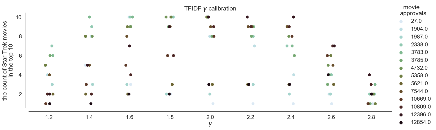
Figure 3: The calibration experiment results. Each dot represents the top 10 count value (vertical axis) when searching for a single movie (hue represents the popularity of the movie, the darker the more approvals the movie has) using TF-IDF with a given $\gamma$ (horizontal axis).

We used each Star Trek movie as a singleton query set, computed its local approval election, ranked the movies from this election with respect to their TF-IDF values for $\gamma\in\{1.2,1.4,1.6,$ $1.8,2.0,2.2,2.4,2.6,2.8\}$, and for each of these values of $\gamma$ calculated how many other Star Trek movies are among the top ten ones. We present the results in Figure 3. The interpretation of this figure is as follows. For each value of $\gamma$, we present all the 14 Star Trek movies as dots. The $y$ coordinate of each dot is the number of other Star Trek movies that are among top-ten ones when we use the given movie as a singleton query set. The color of each dot corresponds to the number of approvals it receives in the global election. Finally, we have averaged the $y$ coordinates of the fourteen movies for each value of $\gamma$ and present the results in Table 2(b). It turned out that $\gamma=2$ indeed gave the best results (naturally, doing a more fine-grained search for the value of $\gamma$ might lead to a slightly different outcome, but we did not feel it would affect the other results in the paper significantly).

While setting $\gamma=2$ works well for many movies, it is not as good a choice for some others. Consider Figure 2 which is analogous to Figure 2, but for the movie Star Trek: Renegades (2015), which is not very popular and its local approval election contains relatively few movies (dots on the diagram). Note that taking $\gamma=2$ does not seem to strike the right balance and we would need to choose $\gamma$ between $1.2$ and $1.6$. Nevertheless, we choose the simplicity of choosing a single value of the $\gamma$ parameter for all the movies, at the cost of getting a few of them wrong.

4.2 Focus Versus Breadth: Synthetic Data

In the second experiment we generate the global election synthetically, so that it resembles data regarding movies. The point is to observe the differences between committees computed according to $p$-HUV rules for different values of $p$ in a controlled environment.

Generating Global Elections.

We assume that we have nine main categories of movies (such as, e.g., a comedy or a thriller) and each category has nine subcategories (such as, e.g., a romantic comedy, or a psychological thriller). For each pair of a category $u\in\{1,\ldots,9\}$ and its subcategory $v\in\{1,\ldots,9\}$, we generate $25$ movies, denoted $u.v(1),\ldots,u.v(25)$. Given a movie $u.v(i)$, we set its quality factor to be $q(i)=-\arctan{\frac{i-13}{10}}+2$. That is, for each subcategory the first movie has the highest quality, about $2.87$, and the qualities of the following movies decrease fairly linearly, down to about $1.12$. We also have $n=2000$ voters. Each voter $i$ has a probability distribution $P_{i}$ over the main categories (where we interpret $P_{i}(u)$ as the probability that the voter watches a movie from category $u$), and for each category $u$, he or she has probability distribution $P_{i}^{u}$ over its subcategories (interpreted as the conditional probability that if the voter watches a movie from category $u$, then this movie’s subcategory is $v$). For each voter, we choose these distributions as permutations of:

$$(0.5,0.1,0.1,0.1,0.1,0.025,0.025,0.025,0.025)$$

chosen uniformly at random. Intuitively, each voter has his or her most preferred category, four categories that he or she also quite enjoys, and four categories that he or she rarely enjoys (the same applies to subcategories). To generate an approval of a voter $i$ we do as follows:

1. We choose a category $u$ according to distribution $P_{i}$ and, then, a subcategory $v$ according to distribution $P_{i}^{u}$.

2. We choose a movie among $u.v(1),\ldots,u.v(25)$ with probability proportional to its quality factor. The voter approves the selected movie.

We repeat this process 162 times for each voter, leading to a bit fewer approvals (due to repetitions in sampling; recall that in MovieLens the average number of approvals is 154).

While the above-described process of generating a global election is certainly quite ad-hoc, we believe that it captures some of the main features of people’s preferences regarding movies. More importantly, we can say that two movies are very similar if they come from the same subcategory, are somewhat similar if they come from the same category but different subcategories, and are very loosely related otherwise.

Figure 4: Visual arrangement of the movie categories and subcategories for the synthetic experiment.

Running The Experiment.

For each number $p\in\{0,1,2,3\}$ and both algorithms for computing approximate $p$-HUV committee (i.e., the greedy algorithm and simulated annealing) we repeat the following experiment. We generate $100$ global elections as described above, and for each of them we compute a committee of size $k=10$ for the query set consisting of movie $1.1(13)$, i.e., the middle-quality movie from subcategory $1.1$ (since the (sub)categories are, effectively, symmetric, their choice is irrelevant). Altogether, $1000$ movies are selected (some of the movies are selected more than once and we count each of them). Then, for each subcategory $u.v$, we sum up, over all the computed committees, how many movies from this subcategory were selected, obtaining a histogram (in this respect, our experiment is quite similar to that of Elkind et al. (2017a)).

To present these histograms visually, we arrange the categories into a $3\times 3$ square, where each category is further represented as a $3\times 3$ subsquare of subcategories, as shown in Figure 4. We show thus-arranged histograms for simulated annealing in Figure 6 and for the greedy algorithm in Figure 6. Each subcategory square is labeled with the number of movies selected from this subcategory and its background reflects this number (darker backgrounds correspond to higher numbers). Further, in both figures next to the name of each $p$-HUV rule we report a vector $(x,y,z)$, where $x$ means the number of movies selected from subcategory $1.1$, $y$ means the number of movies selected from category $1$ except for those in subcategory $1.1$, and $z$ refers to the number of all the other selected movies. Thus we always have that $x+y+z=1000$.

(a) $0$-HUV, ${(979,20,1)}$

(b) $1$-HUV, ${(637,230,133)}$

(c) $2$-HUV, ${(392,261,347)}$

(d) $3$-HUV, ${(301,258,441)}$

Figure 5: Histograms for the synthetic experiment and simulated annealing.

(e) $0$-HUV, ${(982,17,1)}$

(f) $1$-HUV, ${(651,232,117)}$

(g) $2$-HUV, ${(434,262,304)}$

(h) $3$-HUV, ${(338,254,408)}$

Figure 6: Histograms for the synthetic experiment and the greedy algorithm.

Analysis.

Our main conclusion is that, indeed, $0$-HUV focuses on very similar movies (almost all the selected movies come from category $1.1$) and as $p$ increases, approximate $p$-HUV committees include more and more movies from other subcategories of category $1$, and, eventually, even more movies outside of it. It would be desirable to have a value of $p$ for which we would get a vector $(x,y,z)$ close to, say, $(450,450,100)$, meaning that, on average, the resulting committee would contain between $4$ and $5$ movies from category $1.1$ (i.e., directly relevant to the search), between $4$ and $5$ movies from other subcategories of category $1$ (i.e., similar but quite different from the query), and $1$ movie from some other category (i.e., something very different, but possibly appealing to the people who enjoyed the movie from the query). Yet, our algorithms do not seem to provide committees with such vectors (this, however, is not a major worry—after all, the setup in the experiment was simplified and, to some extent, Example 6 shows that for real-life MovieLens data we do find such committees).

4.3 Focus Versus Breadth: Movies Data

In this section we observe how varying the value of $p$ affects the results of $p$-HUV rules on the MovieLens dataset. Ideally, we would like to see the same transition from very focused to quite broad results as with synthetic data. To this end, we first need a methodology for analyzing similarity between movies. We focus on the greedy algorithm for computing $p$-HUV rules as the results for simulated annealing would be very similar.

Similarity Among Movies.

Let us consider two movies, $x$ and $y$. We take the following approach to obtain a number that, in some way, is related to their similarity. First, we form a local utility election using $x$ as the singleton query set (to maintain symmetry, later we will do the same for $y$). If $y$ does not appear in this election, then we consider it as completely dissimilar from $x$. Otherwise, we sort the movies from the local election in the ascending order of their TF-IDF values (as before, we use $\gamma=2$) and we define the rank of $y$ with respect to $x$, denoted ${{\mathrm{rank}}}_{x}(y)$ to be the position on which $y$ appears. (So if $y$ has the highest TF-IDF value then ${{\mathrm{rank}}}_{x}(y)=1$, if it has the second highest TF-IDF then ${{\mathrm{rank}}}_{y}(x)=2$, and so on; recall that the idea of TF-IDF is that the higher it is, the more relavant a movie is for the search query and, so, we equate relevance with similarity). We define the dissimilarity between $x$ and $y$ as:

$${{\mathrm{diss}}}(x,y)=\nicefrac{{1}}{{2}}\big{(}{{\mathrm{rank}}}_{x}(y)+{{\mathrm{rank}}}_{y}(x)\big{)}.$$

This definition ensures that ${{\mathrm{diss}}}(x,y)={{\mathrm{diss}}}(y,x)$ and that the larger ${{\mathrm{diss}}}(x,y)$ is, the less related—and, hence, less similar—are the two movies. However, it also has some flaws. For example, let us consider two sets of movies, $A$ and $B$, where the movies in each of the sets are very similar to each other. Further, let us assume that $A$ contains significantly more movies than $B$. Then the average dissimilarity between the movies in $A$ would be considerably larger than the dissimilarity between the movies in $B$, even if objectively there would be no justification for such a difference. While we acknowledge that such issues may happen, we view them as somewhat extreme and we expect that in most situations our measure is sufficient to distinguish between movies that are clearly related and those that do not have much to do with each other.

Gathering Movies for Comparison.

We would like to compare the outcomes of various $p$-HUV rules on each of the movies from some set $A$. To do so, we form an extension of $A$ as follows (we consider $p$ values in $\{0,1,2,3\}$ and committee size $k=10$, unless we say otherwise):

1. For each movie $x\in A$ and each $p\in\{0,1,2,3\}$, we compute the $p$-HUV winning committee for the local utility election based on the singleton query $x$. We take the union of these committees and call it $B$.

2. For each movie $y\in B$, we compute $0$-HUV winning committee of size two for the local utility election based on $y$. We refer to the union of these committees as $C$.

3. We declare ${{\mathrm{ext}}}(A)=A\cup B\cup C$ to be the extension of $A$.

We use set $B$ because we are interested in relations between the contents of the committees provided by all our rules for all the movies in $A$, and we add set $C$ because we also want to ensure that for each member of one of the committees there also are some very similar movies in the extension.

Visualizing Relations Between the Movies.

Given a set $A$ of movies and its extension ${{\mathrm{ext}}}(A)$, we first compute the value ${{{\mathrm{diss}}}}(x,y)$ for all distinct movies $x$ and $y$ in ${{\mathrm{ext}}}(A)$. Then, we form a complete graph where members of ${{\mathrm{ext}}}(A)$ are the nodes and for each two movies $x$ and $y$, the edge connecting them has weight ${{{\mathrm{diss}}}}(x,y)$. Then we compute an embedding that maps each movie in ${{\mathrm{ext}}}(A)$ to a point on a two-dimensional plane, so that the Euclidean distances between these points correspond to the weights of the edges. To this end, we use the force-directed algorithm of Fruchterman and Reingold (1991). We use an implementation of the algorithm as provided in the networkx library (networkx.drawing.layout.spring_layout, version $2.6.3$), ran for 10’000 iterations. For a description of the library we refer the reader to Hagberg et al. (2008).

As input the Fruchterman-Reingold algorithm does not take the weights of the edges in the graph whose embedding it is to compute, but the forces that act to bring the nodes of a given edge closer. Since this value should be inverse to our dissimilarity, for each two movies $x$ and $y$ we use force $({{{\mathrm{diss}}}}(x,y))^{-2}$ (i.e., we use the square of the inversed dissimilarity; by experimenting with different force functions we found this value to work well).

Experiment 1: Comparing $\boldsymbol{p}$-HUV Rules.

Figure 7: Embedding of the movies in Experiment 1.

Next we use the visualization methodology to analyze the outcomes of different $p$-HUV rules. We let the set $A$ consist of the following movies: Hot Shots! (1991), Ring, The (2002), Star Trek V: The Final Frontier (1989), Star Trek: Generations (1994), Alien (1979), and Dirty Dozen, The (1967). We chose these movies because they represent different genres and styles. Hot Shots! is a quirky comedy, The Ring is a horror movie, Star Trek movies are examples of science-fiction, and so is Alien which also has strong elements of a horror movie. Finally, The Dirty Dozen is a classic war movie. We show an embedding of these movies (and the movies from their extension) in Figure 7. In particular, we see that the two Star Trek movies are correctly presented as very similar, whereas the other movies are farther away from each other.

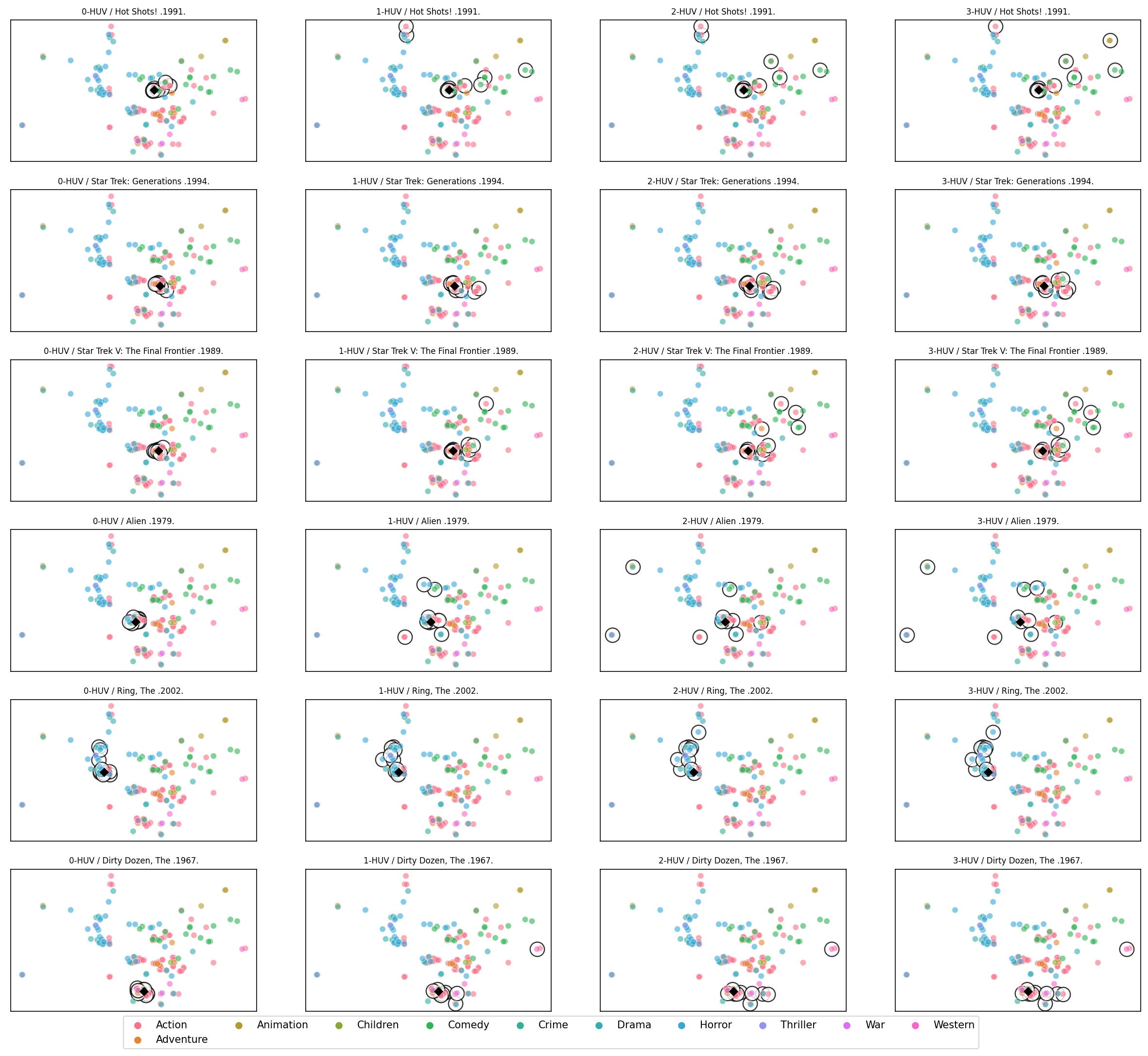
Figure 8: Committees computed using $p$-HUV rules for different queries from Experiment 1.

In Figure 8 we visualize the committees provided by $p$-HUV rules for $p\in\{0,1,2,3\}$ and singleton query sets from $A$. Specifically, each column corresponds to a value of $p$ and each row to a different query. The members of selected committees have surrounding black circles. The movies are colored with respect to the first genre provided for it in MovieLens (in this dataset each movie can have multiple genres, listed in some order).

We make several observations. First, we see that the $0$-HUV rule always chooses movies very close (very similar) to the one from the query. This is hardly surprising as, in essence, we have defined our dissimilarity function to encode this effect. Thus it is more interesting to consider $p$-HUV rules for $p\geq 1$. In this case, we see that the selected movies are always farther away from the query than for $0$-HUV, but the extent to which this happens varies. For example, for Hot Shots! the committees get more and more spread as $p$ increases, whereas for Star Trek: Generations the outcomes are very similar for all $p\geq 1$. It is also quite striking that there is very little difference between $2$-HUV and $3$-HUV for all the six movies. Yet, altogether, we can say that our system achieves its main goals. The $0$-HUV rule gives tightly focused results, closely connected to the query, and $p$-HUV rules for $p\geq 1$ give more diverse results.

Experiment 2: Indiana Jones and Star Trek Movies

The second experiment provides a somewhat anectodical evidence that our dissimilarity measure can identify interesting features of our data. In this case, we first let $A$ consists of four movies about Indiana Jones, an adventurer arachaeologist. These movies are: Indiana Jones and the Raiders of the Lost Ark (1981), Indiana Jones and the Temple of Doom (1984), Indiana Jones and the Last Crusade (1989), Indiana Jones and the Kingdom of the Crystal Skull (2008). We show the visualization of the extension of this set of movies in Figure 9(a).

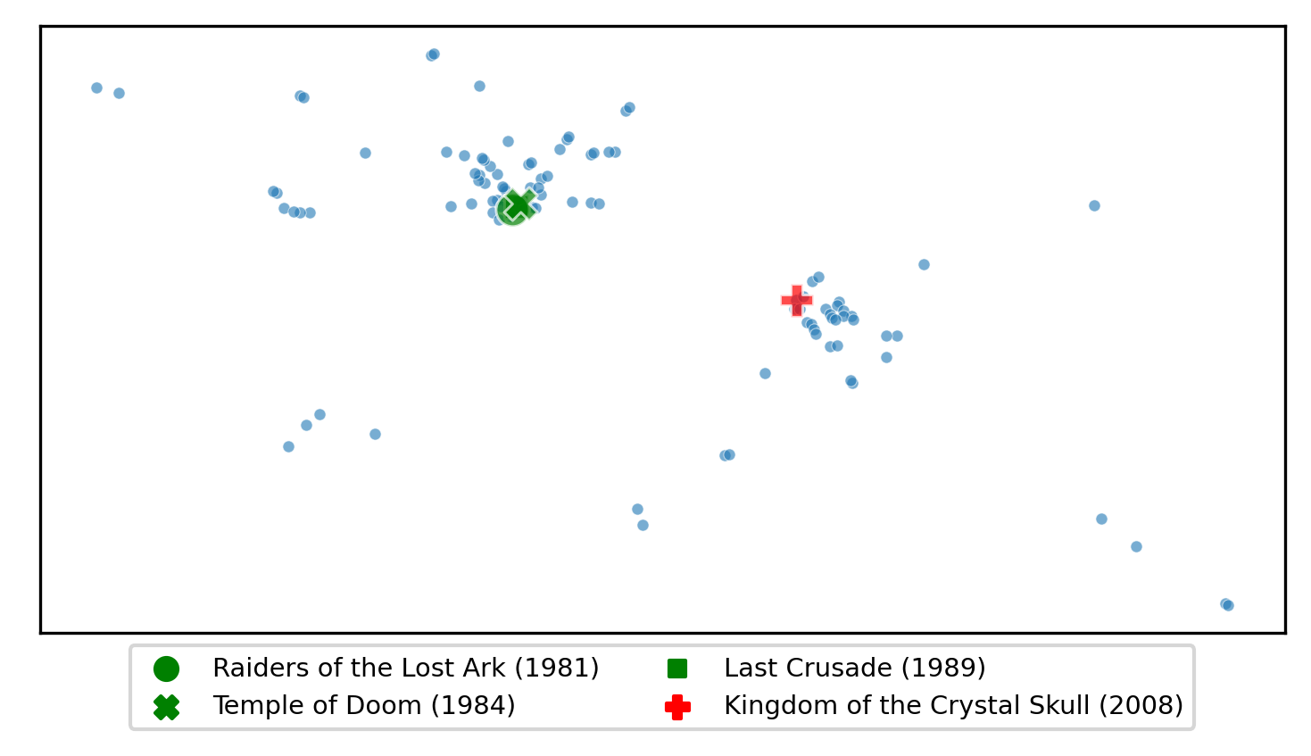
(a) Indiana Jones movies.

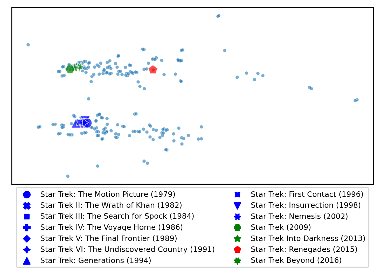
(b) Star Trek movies.

Figure 9: Embeddings for Experiment 2.

We see that the original trilogy, filmed in the 80s, is placed close together, whereas the new movie from 2008 is quite far away. Indeed, as one may expect, reviving of Indiana Jones franchise after nineteen years resulted in very mixed reactions from the fans. We find it quite interesting that such phenomena are visible in our dissimilarity measure. Yet, the readers may wonder if the difference between the Indiana Jones movies can simply be explained by the difference in their release dates. After all, it is quite natural that much older movies might be approved by different sets of people than newer ones. This, of course, might be the case, but it certainly is not the only explanation.

To see that the release date may not influence similarity as much, let us consider the Star Trek movies, as listed in Table 2(a), which were released between 1979 and 2016. We show their embedding in Figure 9(b). We see that the first ten movies, released between 1979 and 2002 (i.e., over a period of over twenty years) and marked with blue symbols, are clustered closely together. These movies form the original series together with The Next Generation series (the transition between the two series was quite gentle, hence it is not surprising that the two groups of movies come together). The next cluster consists of three movies from 2009, 2013, and 2016 and is marked in green. These movies form a new, reboot series (so-called Kelvin Timeline). Finally, the 2015 movie is a fan film and does not belong to the official set of movies. Altogether, we see that similar movies are grouped together even if they were released over a long period of time, whereas significant changes, such as making a reboot or shooting a fan film, are clearly separated.

4.4 Effectiveness of the Approximations

In the final experiment we compare the quality of the committees computed by the greedy algorithm and by simulated annealing, for the MovieLens dataset. To this end, we sampled $1000$ movies and used them as singleton query sets. For each we have computed the local utility election computed approximate winning committees for $1$-HUV, $2$-HUV, and $3$-HUV, using both our algorithms. For each movie we calculated the ratio of the score computed using the greedy algorithm and simulated annealing (so if the ratio is above $1$ then the greedy algorithm performs better and if it is below $1$, then simulated annealring is better). We show the results in Figure 10(a) and, in a more aggregate form, in Figure 4.4. On average, the greedy algorithm finds committees with about $3\%$ higher scores than simulated annealing. Yet, as we have seen in Example 6, simulated annealing has other positive features. We note that we ran the simulated annealing algorithm for $50000$ steps and using more would certainly improve the result (yet, simulated annealing already takes four times as long to compute as the greedy algorithm). All in all, we conclude that both algorithms perform comparably well.

(a) Effectiveness of the greedy algorithm versus simulated annealing. Each dot represents a single movie (from a set of 1000 randomly selected ones), and is used as a singleton query set. Its position on the $y$ axis is the ratio of the scores of the committees computed for this movie using the greedy algorithm and simulated annealing. The position on the $x$-axis is perturbed to show all the dots. The color of the dot represents the number of approvals of the movie in the global election (the darker it is, the more approvals).

rule	Mean	Std. Dev.
1-HUV	1.029	0.028
2-HUV	1.030	0.027
3-HUV	1.031	0.028

(b) Average ratios of committee scores computed using the greedy algorithm and using the simulated annealing algorithm. We provide both the mean values of the scores and their standard deviations.

(c) Effectiveness of our algorithms of the MovieLens 25M dataset.

5 Conclusions

We have shown that multiwinner voting can be successfully used to build a system that helps searching for movies and that lets the users specify how strongly related should the proposed set of movies be to those he or she asks about. Interestingly, our approach can be used to identify nonobvious relations between the movies (as we have observed for the case of Indiana Jones and Star Trek series of movies). Our system does not use any advanced tools for non-personalized recommendation systems and purely demonstrates that multiwinner voting is something that designers of such systems might want to consider.

We do not discuss running times of our algorithms. They are implemented using Python and are highly non-optimized, so analyzing their running times would not be very meaningful.

Acknowledgments

Grzegorz Gawron was supported in part by AGH University of Science and Technology and the "Doktorat Wdrożeniowy" program of the Polish Ministry of Science and Higher Education. This project has received funding from the European Research Council (ERC) under the European Union’s Horizon 2020 research and innovation programme (grant agreement No 101002854).

References

- (1)
- Azaria et al. (2013) A. Azaria, A. Hassidim, S. Kraus, A. Eshkol, O. Weintraub, and I. Netanely. 2013. Movie Recommender System for Profit Maximization. In Proceedings of RecSys-13. 121–128.
- Aziz et al. (2017) H. Aziz, M. Brill, V. Conitzer, E. Elkind, R. Freeman, and T. Walsh. 2017. Justified Representation in Approval-Based Committee Voting. Social Choice and Welfare 48, 2 (2017), 461–485.
- Aziz et al. (2015) H. Aziz, S. Gaspers, J. Gudmundsson, S. Mackenzie, N. Mattei, and T. Walsh. 2015. Computational Aspects of Multi-Winner Approval Voting. In Proceedings of AAMAS-15. 107–115.
- Betzler et al. (2013) N. Betzler, A. Slinko, and J. Uhlmann. 2013. On the Computation of Fully Proportional Representation. Journal of Artificial Intelligence Research 47 (2013), 475–519.
- Bredereck et al. (2020) R. Bredereck, P. Faliszewski, A. Kaczmarczyk, D. Knop, and R. Niedermeier. 2020. Parameterized Algorithms for Finding a Collective Set of Items. In Proceedings of AAAI-20. 1838–1845.
- Brill et al. (2018) M. Brill, J.-F. Laslier, and P. Skowron. 2018. Multiwinner Approval Rules as Apportionment Methods. Journal of Theoretical Politics 30, 3 (2018), 358–382.
- Celis et al. (2016) L Elisa Celis, Amit Deshpande, Tarun Kathuria, and Nisheeth K Vishnoi. 2016. How to be fair and diverse? arXiv preprint arXiv:1610.07183 (2016).
- Celis et al. (2017) L Elisa Celis, Lingxiao Huang, and Nisheeth K Vishnoi. 2017. Multiwinner voting with fairness constraints. arXiv preprint arXiv:1710.10057 (2017).
- Chakraborty et al. (2019) A. Chakraborty, G. Patro, N. Ganguly, K. Gummadi, and P. Loiseau. 2019. Equality of Voice: Towards Fair Representation in Crowdsourced Top-K Recommendations. In Proceedings of FAT-19. 129–138.
- Chamberlin and Courant (1983) B. Chamberlin and P. Courant. 1983. Representative Deliberations and Representative Decisions: Proportional Representation and the Borda Rule. American Political Science Review 77, 3 (1983), 718–733.
- Chasalow and Levy (2021) Kyla E. Chasalow and Karen E. C. Levy. 2021. Representativeness in Statistics, Politics, and Machine Learning. Proceedings of the 2021 ACM Conference on Fairness, Accountability, and Transparency (2021).
- Choi et al. (2012) S. Choi, S. Ko, and Y. Han. 2012. A Movie Recommendation Algorithm Based On Genre Correlations. Expert Systems with Applications 39, 9 (2012), 8079–8085.
- Clarke et al. (2008) Charles LA Clarke, Maheedhar Kolla, Gordon V Cormack, Olga Vechtomova, Azin Ashkan, Stefan Büttcher, and Ian MacKinnon. 2008. Novelty and diversity in information retrieval evaluation. In Proceedings of the 31st annual international ACM SIGIR conference on Research and development in information retrieval. 659–666.
- Drosou et al. (2017) Marina Drosou, HV Jagadish, Evaggelia Pitoura, and Julia Stoyanovich. 2017. Diversity in big data: A review. Big data 5, 2 (2017), 73–84.
- Elkind et al. (2017a) E. Elkind, P. Faliszewski, J. Laslier, P. Skowron, A. Slinko, and N. Talmon. 2017a. What Do Multiwinner Voting Rules Do? An Experiment Over the Two-Dimensional Euclidean Domain. In Proceedings of AAAI-17. 494–501.
- Elkind et al. (2017b) E. Elkind, P. Faliszewski, P. Skowron, and A. Slinko. 2017b. Properties of Multiwinner Voting Rules. Social Choice and Welfare 48, 3 (2017), 599–632.
- Faliszewski et al. (2017a) P. Faliszewski, J. Sawicki, R. Schaefer, and M. Smolka. 2017a. Multiwinner Voting in Genetic Algorithms. IEEE Intelligent Systems 32, 1 (2017), 40–48.
- Faliszewski et al. (2017b) P. Faliszewski, P. Skowron, A. Slinko, and N. Talmon. 2017b. Multiwinner Rules on Paths From -Borda to Chamberlin–Courant. In Proceedings of IJCAI-17. 192–198.
- Faliszewski et al. (2017c) P. Faliszewski, P. Skowron, A. Slinko, and N. Talmon. 2017c. Multiwinner Voting: A New Challenge for Social Choice Theory. In Trends in Computational Social Choice, U. Endriss (Ed.). AI Access Foundation.
- Faliszewski et al. (2017d) Piotr Faliszewski, Piotr Skowron, Arkadii Slinko, and Nimrod Talmon. 2017d. Multiwinner voting: A new challenge for social choice theory. Trends in computational social choice 74, 2017 (2017), 27–47.
- Fruchterman and Reingold (1991) T. Fruchterman and E. Reingold. 1991. Graph Drawing by Force-Directed Placement. Software: Practice and Experience 21, 11 (1991), 1129–1164.
- Ghosh et al. (1999) Sumit Ghosh, Manisha Mundhe, Karina Hernandez, and Sandip Sen. 1999. Voting for movies: the anatomy of a recommender system. In Proceedings of the third annual conference on Autonomous Agents. 434–435.
- Godziszewski et al. (2021) M. Godziszewski, P. Batko, P. Skowron, and P. Faliszewski. 2021. An Analysis of Approval-Based Committee Rules for 2D-Euclidean Elections. In Proceedings of AAAI-21. 5448–5455.
- Hagberg et al. (2008) Aric Hagberg, Pieter Swart, and Daniel S Chult. 2008. Exploring network structure, dynamics, and function using NetworkX. Technical Report. Los Alamos National Lab.(LANL), Los Alamos, NM (United States).
- Harper and Konstan (2016) F. M. Harper and J. Konstan. 2016. The MovieLens Datasets: History and Context. ACM Transactions on Interactive Intelligent Systems 5, 4 (2016), 19:1–19:19.
- Järvelin and Kekäläinen (2002) Kalervo Järvelin and Jaana Kekäläinen. 2002. Cumulated gain-based evaluation of IR techniques. ACM Transactions on Information Systems (TOIS) 20, 4 (2002), 422–446.
- Jones (1973) K. Spärck Jones. 1973. Index Term Weighting. Information Storage and Retrieval 9, 11 (1973), 619–633.
- Jones (2004) K. Spärck Jones. 2004. A Statistical Interpretation of Term Specificity And Its Application In Retrieval. Journal of Documentation 60, 5 (2004), 493–502.
- Kim et al. (2019) Y. Kim, K. Kim, C. Park, and H. Yu. 2019. Sequential and Diverse Recommendation with Long Tail. In Proceedings of IJCAI-19. 2740–2746.
- Lackner and Skowron (2018) M. Lackner and P. Skowron. 2018. Consistent Approval-Based Multi-Winner Rules. In Proceedings of EC-18. 47–48.
- Lackner and Skowron (2020a) M. Lackner and P. Skowron. 2020a. Approval-Based Committee Voting: Axioms, Algorithms, and Applications. Technical Report arXiv:2007.01795 [cs.GT]. arXiv.org.
- Lackner and Skowron (2020b) M. Lackner and P. Skowron. 2020b. Utilitarian Welfare and Representation Guarantees of Approval-Based Multiwinner Rules. Artificial Intelligence 288 (2020), 103366.
- Leung (2018) CK Leung. 2018. Encyclopedia of Database Systems.
- Mitchell et al. (2020) Margaret Mitchell, Dylan Baker, Nyalleng Moorosi, Emily Denton, Ben Hutchinson, Alex Hanna, Timnit Gebru, and Jamie Morgenstern. 2020. Diversity and inclusion metrics in subset selection. In Proceedings of the AAAI/ACM Conference on AI, Ethics, and Society. 117–123.
- Mondal et al. (2020) A. Mondal, R. Bal, S. Sinha, and G. Patro. 2020. Two-Sided Fairness in Non-Personalised Recommendations. Technical Report arXiv:2011.05287 [cs.AI]. arXiv.org.
- Nemhauser et al. (1978) G. Nemhauser, L. Wolsey, and M. Fisher. 1978. An Analysis of Approximations for Maximizing Submodular Set Functions. Mathematical Programming 14, 1 (Dec. 1978), 265–294.
- Ounis (2018) I. Ounis. 2018. Inverse Document Frequency. In Encyclopedia of Database Systems. Springer.
- Peters and Lackner (2020) D. Peters and M. Lackner. 2020. Preferences Single-Peaked on a Circle. Journal of Artificial Intelligence Research 68 (2020), 463–502.
- Phonexay et al. (2018) V. Phonexay, D. Park, K. Xinchang, and F. Hao. 2018. An Efficient Movie Recommendation Algorithm Based On Improved -Clique. Human-centric Computing and Information Sciences 8 (2018), 38.
- Pourghanbar et al. (2015) M. Pourghanbar, M. Kelarestaghi, and F. Eshghi. 2015. EVEBO: A New Election Inspired Optimization Algorithm. In Proceedings of CEC-15. 916–924.
- Procaccia et al. (2008) A. Procaccia, J. Rosenschein, and A. Zohar. 2008. On the Complexity of Achieving Proportional Representation. Social Choice and Welfare 30, 3 (2008), 353–362.
- Ricci et al. (2015) F. Ricci, L. Rokach, and B. Shapira (Eds.). 2015. Recommender Systems Handbook. Springer.
- Robertson and Walker (1997) S. Robertson and S. Walker. 1997. On Relevance Weights with Little Relevance Information. In Proceedings of SIGIR-97. 16–24.
- Sarwar et al. (2001) B. Sarwar, G. Karypis, J. Konstan, and J. Riedl. 2001. Item-Based Collaborative Filtering Recommendation Algorithms. In Proceedings of WWW-01. 285–295.
- Skowron et al. (2016) P. Skowron, P. Faliszewski, and J. Lang. 2016. Finding a collective set of items: From proportional multirepresentation to group recommendation. Artificial Intelligence 241 (2016), 191–216.
- Thiele (1895) T. Thiele. 1895. Om Flerfoldsvalg. In Oversigt over det Kongelige Danske Videnskabernes Selskabs Forhandlinger. 415–441.
- Yager (1988) R. Yager. 1988. On Ordered Weighted Averaging Aggregation Operators in Multicriteria Decisionmaking. IEEE Transactions on Systems, Man and Cybernetics 18, 1 (1988), 183–190.