Linked Cluster Expansions via Hypergraph Decompositions

Abstract

We propose a hypergraph expansion which facilitates the direct treatment of quantum spin models with many-site interactions via perturbative linked cluster expansions. The main idea is to generate all relevant subclusters and sort them into equivalence classes essentially governed by hypergraph isomorphism. Concretely, a reduced König representation of the hypergraphs is used to make the equivalence relation accessible by graph isomorphism. During this procedure we determine the embedding factor for each equivalence class, which is used in the final resummation in order to obtain the final result. As an instructive example we calculate the ground-state energy and a particular excitation gap of the plaquette Ising model in a transverse field on the three-dimensional cubic lattice.

I Introduction

Although graph decomposition methods have been employed already decades ago in order to obtain high-order series expansions of many-body systems Marland (1981); Irving and Hamer (1984); He et al. (1990); Oitmaa et al. (1991); Hamer et al. (1992), they continue to be a state of the art approach to perform calculations for quantum lattice models, for example using perturbative methods like high-temperature series expansions Hehn et al. (2017); Singh and Oitmaa (2017), Rayleigh-Schrödinger perturbation theory Hehn (2016); Oitmaa (2020, 2021), perturbative continuous unitary transformations (pCUTs) Knetter and Uhrig (2000); Knetter et al. (2003); Yang et al. (2010a); Coester et al. (2016); Adelhardt et al. (2020); Schmoll et al. (2020) or non-perturbative numerical tools like exact diagonalization Ixert and Schmidt (2016); Rigol et al. (2006); Schäfer et al. (2020), density matrix renormalization group Stoudenmire et al. (2014), and graph-based continuous unitary transformations Yang and Schmidt (2011); Ixert et al. (2014); Coester et al. (2015) in the context of numerical linked cluster expansions. Historically the graph decomposition methods for high-order series expansions were exclusively applicable to extensive quantities like ground-state energies Marland (1981); Irving and Hamer (1984) or had to take into account also disconnected graphs He et al. (1990); Gelfand (1996). It took some time until it was clear how to set up linked cluster expansions, where only connected graphs have to be considered, for non-extensive quantities like the excitation gap Gelfand (1996), two-particle properties Trebst et al. (2000); Zheng et al. (2001); Knetter et al. (2000) or multi-particle spectral densities Schmidt et al. (2001); Knetter et al. (2001); Hörmann et al. (2018). Detailed reviews on high-order series expansions using graph decomposition techniques can be found in Gelfand and Singh (2000); Oitmaa et al. (2006). While for pairwise interactions it is straightforward to represent the involved clusters in terms of graphs, where the vertices correspond to sites and the edges represent interactions between the sites Joshi et al. (2015); Hehn et al. (2017), this is usually not the case when interactions join multiple sites. However, some problem specific approaches to treat such many-site interactions in topologically ordered phases can be found in the literature Schulz et al. (2013, 2014).

Many-site interactions play an important role for several aspects in quantum many-body systems. In statistical physics, interesting critical properties arise due to three-body interactions like in the Baxter-Wu model Baxter and Wu (1973); Capponi et al. (2014) or quantum phase transitions with fractal properties Zhou et al. (2021). In topological systems, there exist a collection of exactly solvable models with exotic physical properties like topological or fracton order which consist of commuting many-site operators - so called stabilizer codes Gottesman (1997). Famous examples are Kitaev’s toric code Kitaev (2003) and its three-dimensional generalization Hamma et al. (2005); Nussinov and Ortiz (2008); Reiss and Schmidt (2019), color codes Kargarian (2009); Katzgraber et al. (2009), and string-net models Levin and Wen (2005) displaying long-range entangled ground states with topological order or three-dimensional fracton systems like the X-Cube model, the checkerboard model or Haah’s cubic code Haah (2011); Vijay et al. (2016). Another class of stabilizer codes with multi-site interactions are cluster-state Hamiltonians in the context of measurement-based quantum computation Raussendorf and Briegel (2001); Briegel and Raussendorf (2001); Orús et al. (2013). The exact solvability of these stabilizer codes has been the starting point for many fundamental investigations of the physical properties of such systems, e.g. their quantum robustness and associated quantum critical properties. High-order series expansions represent one important tool to study these questions Dusuel et al. (2011); Kalis et al. (2012); Jahromi et al. (2013); Schulz et al. (2013, 2014); Mühlhauser et al. (2020). In condensed matter physics, multi-site interactions are known to arise in strongly correlated Mott insulators like Hubbard systems in the limit of strong interactions MacDonald et al. (1988); Reischl et al. (2004); Yang et al. (2010b, 2012). In unfrustrated materials like the undoped high-$T_{\rm c}$ superconductors or corresponding quasi one-dimensional cuprate ladders, four-spin interactions are needed for a quantitative description of the magnetic properties Windt et al. (2001); Katanin and Kampf (2003); Schmidt et al. (2005); Schmidt and Uhrig (2005); Notbohm et al. (2007). In frustrated Mott insulators like the Hubbard model on the triangular lattice, four-spin interactions are expected to trigger exotic quantum spin liquid phases in the Mott insulating regime Motrunich (2005); Sheng et al. (2009); Yang et al. (2010b); Block et al. (2011); Boos et al. (2020); Szasz et al. (2020).

As a consequence, a general framework for performing linked cluster expansions in quantum many-body systems with multi-site interactions is highly desirable. From a conceptional point of view hypergraphs are a natural generalization of graphs to describe more complex relationships, where edges can connect more than two vertices Berge (1973); Zykov (1974); Berge (1989); Bretto (2013); Ouvrard (2020). Indeed, they have also been employed to represent molecular structures Konstantinova and Skorobogatov (1995, 2001). Additionally, the isomorphism problem for hypergraphs can be solved using conventional graph isomorphism as hypergraphs are uniquely defined by their König representation Zykov (1974); McKay (1981).

In this work we describe how these concepts can be used to perform a graph decomposition for many-site interactions. While in Mühlhauser et al. (2020) we applied a similar technique to study the X-Cube model in a magnetic field, we used the same approach as presented in this work to investigate the competition between the X-Cube and the three dimensional toric code in Mühlhauser et al. (2021) without, however, describing the technical aspects. As a representative example, we apply our scheme to the plaquette Ising model Savvidy et al. (1995); Johnston et al. (2017), in a transverse magnetic field on the three-dimensional cubic lattice Nandkishore and Hermele (2019).

The paper is organized as follows. In Sec. II we describe perturbative linked cluster expansions in the context of pCUTs Knetter and Uhrig (2000); Knetter et al. (2003), as introduced in Coester and Schmidt (2015), with a focus on multi-site interactions. The general aspects of our scheme are contained in Sec. III and it is applied to the plaquette Ising model in a transverse field on the cubic lattice in Sec. IV. Final conclusions are drawn in Sec. V.

II Linked cluster expansions using pCUTs

In this section we review pCUTs in the context of linked cluster expansions based on Coester and Schmidt (2015) focusing on multi-site interactions. For a more detailed introduction to pCUTs we refer to Knetter and Uhrig (2000); Knetter et al. (2003). We consider a lattice Hamiltonian of the form

$$H=H_{0}+\lambda V\,.$$ (1)

Note that one can easily introduce several perturbation parameters $\lambda_{1}\ldots\lambda_{n}$, but we will restrict ourselves to a single perturbation parameter $\lambda$ for the sake of simplicity. For the unperturbed part of the Hamiltonian we make the same assumptions as Coester and Schmidt (2015), i.e. that it can be written as

$$H_{0}=E_{0}+Q=E_{0}+\sum_{i}n_{i}\,,$$ (2)

where $Q$ is the global particle number-operator, $n_{i}$ are local particle-number operators at the site $i$, and $E_{0}$ is a constant. In the example presented in Sec. IV the local degrees of freedom on sites are one type of hardcore boson. However, a site can in principle host systems which feature several degrees of freedom, which are then commonly called supersites. The interaction $V$ contains interactions between these sites. In contrast to the discussion in Coester and Schmidt (2015) we do not restrict ourselves to two-site interactions.

The effective Hamiltonian resulting from pCUTs is given as Knetter and Uhrig (2000); Knetter et al. (2003)

$$H_{\text{eff}}=H_{0}+\sum_{k=1}^{\infty}\lambda^{k}\sum_{\begin{subarray}{c}\vec{m},|\vec{m}|=k\\ \sum_{i}m_{i}=0\end{subarray}}\mathcal{C}(\vec{m})T(\vec{m})\,$$ (3)

with

$$\vec{m} =(m_{1},\ldots,m_{k})\,,$$ (4)

$$|\vec{m}| =\text{dim}(\vec{m})\,,$$ (5)

$$T(\vec{m}) =T_{m_{1}}\ldots T_{m_{k}}$$ (6)

and the $T_{n}$-operators, which create $n$ quasiparticles

$$[Q,T_{n}]=nT_{n}\,.$$ (7)

The most important property of $H_{\text{eff}}$ is $[H_{\text{eff}},Q]=0$ reflecting the quasi-particle conservation. The effective Hamiltonian $H_{\text{eff}}$ is therefore block-diagonal in the number of quasi-particles so that the complicated quantum many-body problem is mapped to an effective few-body problem by pCUTs. This step is model-independent. The model-dependent step of pCUTs is to normal order $H_{\text{eff}}$ in order to extract physical properties like ground-state energies, one-quasi-particle hopping amplitudes or two-quasi-particle interactions. This step is most efficiently done by calculating matrix elements of $H_{\text{eff}}$ on finite clusters exploiting the linked-cluster property of pCUTs.

Obviously, every matrix element of $H_{\text{eff}}$ can be straightforwardly evaluated on a single appropriately chosen cluster, but especially for high-order calculations these clusters tend to become very large making the evaluation of the effective Hamiltonian inefficient Dusuel et al. (2010). At this stage a graph decomposition can be employed to reduce the computational demands. A first step is to realize that the $T_{n}$-operators can be decomposed into local operators Coester and Schmidt (2015)

$$T_{n}=\sum_{b}\tau_{n,b}\,.$$

These local operators usually act only on a small number of sites which are joined by a bond $b$, where they create $n$ quasiparticles. Recall that in order to model many-particle interactions we allow bonds to connect multiple sites. Using this notion, the effective Hamiltonian is rewritten as

$$H_{\text{eff}}=H_{0}+\sum_{k=1}^{\infty}\lambda^{k}\sum_{\begin{subarray}{c}\vec{m},|\vec{m}|=k\\ \sum_{i}m_{i}=0\end{subarray}}\sum_{\vec{b},|\vec{b}|=k}\mathcal{C}(\vec{m})\tau(\vec{m},\vec{b})\,$$ (8)

with

$$\vec{b} =(b_{1},\ldots b_{k})$$ (9)

$$|\vec{b}| =\text{dim}(\vec{b})$$ (10)

$$\tau(\vec{m},\vec{b}) =\tau_{m_{1},b_{1}}\ldots\tau_{m_{k},b_{k}}\,.$$ (11)

Rearranging the sums we can extract the following expression for any bond sequence $\vec{b}$

$$V_{\vec{b}}=\lambda^{|\vec{b}|}\sum_{\begin{subarray}{c}\vec{m},|\vec{m}|=|\vec{b}|\\ \sum_{i}m_{i}=0\end{subarray}}\mathcal{C}(\vec{m})\tau(\vec{m},\vec{b})\,,$$ (12)

and the effective Hamiltonian becomes

$$H_{\text{eff}}=H_{0}+\sum_{\vec{b}}V_{\vec{b}}\,.$$ (13)

Due to the linked cluster property of pCUT the contributions on disconnected subclusters $\mathcal{S}$ vanish Kamfor (2013); Coester and Schmidt (2015). This linked cluster property can be directly understood from the commutator structure of the effective Hamiltonian Dusuel et al. (2010). A bond sequence $\vec{b}$ can be naturally associated to the subcluster of the full system, which exactly contains the bonds which are included in $\vec{b}$. Accordingly, the sum over bond sequences becomes a sum over connected subclusters $\mathcal{S}$

$$H_{\text{eff}} =H_{0}+\sum_{\mathcal{S}}\sum_{\vec{b}\mapsto\mathcal{S}}V_{\vec{b}}$$ (14)

$$=H_{0}+\sum_{\mathcal{S}}V_{\mathcal{S}}\,,$$ (15)

where the subscript $\vec{b}\mapsto\mathcal{S}$ means that the sum runs over all bond sequences $\vec{b}$ associated with the subcluster $\mathcal{S}$. Note that typically many bond sequences are associated to the same subcluster $\mathcal{S}$, since individual bonds can be touched multiple times and in different orders. This implies that evaluating $V_{\mathcal{S}}$ only processes which involve all bonds in $\mathcal{S}$ have to be taken into account.

A crucial next step is to realize, that we do not have to evaluate $V_{\mathcal{S}}$ on every subcluster, but only once for every equivalence class of subclusters. The actual equivalence relation depends on the matrix element $\bra{\Phi}H_{\text{eff}}\ket{\Psi}$ for which the effective Hamiltonian is evaluated. In case $\ket{\Phi},\ket{\Psi}$ are the bare vacuum state ($n_{i}=0\;\forall i$) it is sufficient to identify isomorphic clusters. This is not the case for excited states, as the positions of excitations in the states $\ket{\Phi},\ket{\Psi}$ matter. Generically, a matrix element of the effective Hamiltonian can be written as

$$\bra{\Phi}H_{\text{eff}}\ket{\Psi} =\bra{\Phi}H_{0}\ket{\Psi}+\sum_{\mathcal{E}}N_{\mathcal{E}}\bra{\Phi}V_{\mathcal{S}\in\mathcal{E}}\ket{\Psi}$$ (16)

$$=\bra{\Phi}H_{0}\ket{\Psi}+\sum_{\mathcal{E}}N_{\mathcal{E}}V_{\mathcal{E}}\,,$$

where $\mathcal{S}\in\mathcal{E}$ labels a representative subcluster which is contained in the equivalence class $\mathcal{E}$, and $N_{\mathcal{E}}$ is the number of subclusters contained in $\mathcal{E}$. Obviously, the matrix element $V_{\mathcal{E}}$ can be decomposed, such that one factor is evaluated only on the subcluster, and the other is just the scalar product of the states on the remaining Hilbert space. Accordingly, the effective Hamiltonian is evaluated only on one subcluster per equivalence class, effectively exploiting symmetries of the model and the lattice. The price to pay is, that we have to find all equivalence classes and determine the embedding factors $N_{\mathcal{E}}$ Dusuel et al. (2010), which in the presented approach are essentially obtained by counting the relevant subclusters, i.e. typically one does not have to count all subclusters but one can use process-specific properties like translational invariance for the ground-state energy or the finite extension of linked quantum fluctuations in case of hopping amplitudes.

For the calculation of ground-state expectation values, this graph decomposition approach also works with other methods to evaluate the matrix elements $V_{\mathcal{E}}$ on graphs like Takahashi’s perturbation theory Takahashi (1977); Klagges and Schmidt (2012), Löwdin’s partitioning technique Löwdin (1962); Kalis et al. (2012), or matrix perturbation theory Oitmaa et al. (2006), because the series are unique on any graph and therefore do not depend on the employed method.

III Scheme

The presented scheme consists of two main parts: generating all relevant subclusters and sorting them into equivalence classes based on hypergraph isomorphism. Actually we are doing this on the fly, i.e., whenever we discover a relevant subcluster we check whether we already found an equivalent cluster before. In this way we accumulate a set of equivalence classes while we can also keep track of the corresponding embedding factors. For the sake of simplicity we assume that all bonds in the lattice are symmetry equivalent, and undirected, i.e., the local perturbation acts on all involved sites in the same way. We address in App. A how this scheme can be applied without these assumptions. We further note that a bond does never contain the same site more than once.

It is known that for conventional graphs first generating all relevant isomorphism classes and then calculating the respective embedding factors is more efficient Gelfand and Singh (2000). The presented scheme is no exception. However, our choice is justified taking into account that the generation of hypergraph isomorphism classes appears more challenging compared to the generation of graph isomorphism classes, although it is actually covered in the literature McKay (1998). Even if the problem of finding all relevant hypergraphs was solved, we would still expect the calculation of the embedding factors to be quite time-consuming.

III.1 Generation of relevant subclusters

The generation of subclusters is based on an algorithm presented in Rücker and Rücker (2000), which enumerates all connected subgraphs of a given (conventional) graph. Although this algorithm is described in the literature for conventional graphs the adaption for multi-site interactions described below is straightforward, as the concept to identify a connected subcluster by the set of its bonds is independent of the bond cardinality.

The algorithm starts from a single bond $b_{1}$ and builds connected subclusters by adding further bonds in a depth-first manner Rücker and Rücker (2001). The candidates to be appended are simply the bonds adjacent to the actual subcluster. If a feasible candidate is found, this bond is appended to the subcluster and the algorithm continues with the extended subcluster. The algorithm backtracks if no feasible candidate is found, i.e., it removes the last appended bond and marks it as forbidden. The bond remains forbidden until the algorithm backtracks one step further ensuring that every connected subcluster containing $b_{1}$ is found once and only once Rücker and Rücker (2000). Marking $b_{1}$ as forbidden and restarting the search from another bond $b_{2}$ will yield all connected subclusters which contain $b_{2}$ but do not contain $b_{1}$. So in order to find all connected subclusters the search has to be repeated from all possible starting bonds ignoring all the previous starting bonds during the search Rücker and Rücker (2000).

Obviously, this algorithm can be easily modified to produce all connected subclusters up to a given number of bonds by simply forcing it to backtrack when the maximum size is reached Rücker and Rücker (2000). Additionally, the structure of the search tree makes it easy to incorporate heuristics Oitmaa et al. (2006) to discard unfruitful branches in advance.

For our purpose it is very useful that the algorithm actually allows to generate only the clusters, which intersect with a given set of bonds. For the calculation of hopping amplitudes this helps to only consider clusters which host fluctuations different from vacuum fluctuations, whereas for the calculation of the ground-state energy per bond, this is useful, as we can restrict the set of generated clusters to the clusters which actually contain this bond.

Interestingly, this algorithm has been combined with highly discriminating graph invariants to find all connected non-isomorphic subgraphs of a given graph Rücker and Rücker (2001). However, while this approach yields exact results in some domains, it is only an approximate solution, as the proposed graph invariants were not complete, i.e., there exist non-isomorphic graphs, which have the same invariants Rücker and Rücker (2001); Rücker et al. (2002).

III.2 Sorting subclusters into equivalence classes

In the presented approach subclusters are sorted into equivalence classes based on hypergraph isomorphism. To this end subclusters are associated with the König representation of the corresponding hypergraph. The König representation of a hypergraph is a bipartite graph, where one partition represents the vertices of the hypergraph while the other partition represents the hyperedges Zykov (1974). Whenever a vertex is contained in a hyperedge, an edge connects the corresponding vertices in the bipartite graph. Taking into account the bipartition of the vertex set, this graph represents the hypergraph unambiguously Zykov (1974); Konstantinova and Skorobogatov (1995). Accordingly, this representation enables us to use conventional graph isomorphism to discriminate isomorphism classes of subclusters. An example for the König representation of a hypergraph is shown in Fig. 1 . Note that one can easily distinguish individual sites by coloring the corresponding vertices in the König representation. With this adaption it is also possible to include information about the states involved in a matrix element and so also in this case one can distinguish equivalence classes by graph isomorphism.

In practice, we do not use the full König representation, but a reduced representation, which exploits that the number of sites in all bonds is equal, since we have assumed all bonds to be symmetry equivalent. So vertices of degree one in the vertex partition and adjacent edges can be ignored, if they do not carry any additional information. As a consequence, for calculations of ground-state energies all such vertices can typically be ignored, while for the calculation of hopping amplitudes the distinguished vertices, necessary to encode the initial and the final state of the actual matrix element, have to be kept.

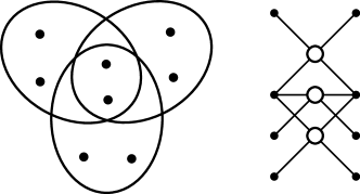
Figure 1: An exemplary hypergraph (left) and its König representation (right). On the left side the black dots correspond to the vertices and the ellipses correspond to the hyperedges linking the included vertices. On the right side the filled vertices correspond to the vertex partition, while the unfilled vertices correspond to the edge-partition i.e., they represent the hyperedges. Vertices from the two partitions are connected if and only if, the respective vertex is contained in the corresponding hyperedge Zykov (1974).

We further perform isomorphism checks with the RI algorithm Bonnici et al. (2013); Bonnici and Giugno (2017) among the resulting graphs. Since such checks are typically rather expensive, we use a combination of graph invariants in order to apply these checks only to graphs which have the same invariants.

While just sorting the relevant subclusters into isomorphism classes is sufficient for the calculation of hopping amplitudes, one still has to apply some corrections for the calculation of the ground-state energy when exploiting symmetries like translations. In a conventional graph decomposition an edge of the graph is typically fixed to a certain bond in the lattice in order to remove redundancies due to existing symmetries like translations. In our approach, this corresponds to the requirement that this bond in the lattice has always a canonical location in the subclusters. If this requirement is not fulfilled on a subcluster, it is not counted as a valid embedding. We will not further elaborate on the details here, but refer to the example presented in Sec. IV, where we also comment on how to keep track of the embedding factors.

IV Application

In this section we treat the plaquette Ising model Savvidy and Wegner (1994); Johnston et al. (2017) in a transverse magnetic field on the cubic lattice Nandkishore and Hermele (2019) as a representative example. The Hamiltonian is given as

$$H=-\sum_{i}\sigma^{z}_{i}-\lambda\sum_{\square}\sigma_{i_{1}}^{x}\sigma_{i_{2}}^{x}\sigma_{i_{3}}^{x}\sigma_{i_{4}}^{x}\,,$$ (17)

where $\square$ indicates that the sum runs over all plaquettes in the lattice, and the indices $i_{1},\ldots i_{4}$ refer to the four sites at the corners of the respective plaquette. Interestingly, this model is dual to the relevant low-energy sector of the fractonic X-Cube model in a $z$-field Vijay et al. (2016); Nandkishore and Hermele (2019). For this case we already obtained series expansions for the ground-state energy and excitations gaps of one- and two-particle excitations Mühlhauser et al. (2020). For the ground-state energy we also compared to quantum Monte Carlo simulations received from Trithep Devakul Devakul et al. (2018) which are also displayed in Mühlhauser et al. (2020). In the latter work we also made the first steps using graph decomposition techniques for fracton models. In the following we aim at treating this model about the high-field limit $\lambda\ll 1$ using high-order linked-cluster expansions. We will start by discussing how to calculate the ground-state energy using the presented approach in large detail. Afterwards we will briefly comment on how this scheme can be adapated to calculate hopping elements of quasiparticle excitations.

IV.1 Ground-state energy

The ground state of the unperturbed system $\lambda=0$ is given by the polarized state

$$\ket{\mathrm{GS}}=\ket{\uparrow\ldots\uparrow}\,.$$ (18)

The action of each four-spin interaction in the perturbation flips the four $\sigma^{z}$-eigenvalues at the four sites of a plaquette.

IV.1.1 Mapping clusters to graphs

First, we observe that bonds always connect four sites. Hence, the common interpretation of bonds as edges of a graph is hardly possible. At this point it is tentative to search for straightforward mappings. For the present problem a naive approach would consist in representing each plaquette by a vertex, and connecting pairs of these vertices by colored edges where the edge color encodes the amount of sites shared by the respective plaquettes. This naive mapping to conventional graphs already fails for clusters involving three plaquettes (see Fig. 2 for a counterexample). Obviously, if such a simple mapping is sufficiently discriminating for the problem at hand, it will very likely outperform the presented method. However, it is not always easy to find such a mapping and there can be some subtle pitfalls.

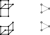
Figure 2: On the left side two subclusters are given, while on the right side their representation using the naive approach presented in the text is illustrated. Empty circles represent plaquettes and they are connected because they have two common sites (another edge color could be used if they would share one site only). In this naive approach the above sublusters would be errorneously classified as equivalent.

Instead, we interpret the plaquettes as edges of a hypergraph, and use the König representation of this hypergraph to represent the isomorphism class of the subcluster. The relevant isomorphism classes up to two plaquettes are given in Fig. 3, while the classes for three plaquettes are illustrated in Fig. 4, showing that the presented approach correctly discriminates the two subclusters in Fig. 2. Clearly, using the full König graph will be very inefficient, especially in cases where bonds connect many sites. However, we can easily reduce the representation, by simply omitting vertices from the vertex partition which have degree one and the adjacent edges. In Figs. 3 and 4 it can be seen in the right column how this reduced representation simplifies the involved graphs.

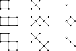
Figure 3: Different isomorphism classes of subclusters up to two plaquettes. In the left column subclusters are given as found in the actual lattice i.e. every plaquette corresponds to a bond, which links the four included sites. The central column is the König representation of the corresponding hypergraph. The right column gives a reduced König representation, which we can use here, because we know that all bonds have cardinality four, and that we do not have to distinguish the sites, because the ground state is simply a polarized state.

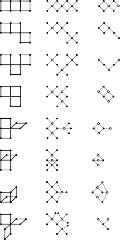
Figure 4: Different isomorphism classes of subclusters with three plaquettes. The columns are explained as in Fig. 3. In the left column subclusters are given as found in the actual lattice i.e. every plaquette corresponds to a bond, which links the four included sites. The central column is the König representation of the corresponding hypergraph. The right column gives a reduced König representation, which we can use here, because we know that all bonds have cardinality four, and that we do not have to distinguish the sites, because the ground state is simply a polarized state. In this order the involved graphs become more complicated and already at this stage a naive approach starts to fail, as shown in Fig. 2.

IV.1.2 Identifying non-contributing clusters

Another important consideration is to identify and discard subclusters which cannot contribute as early as possible. Heuristics to discard non-contributing clusters can be found in He et al. (1990); Oitmaa et al. (2006); Coester (2011); Joshi et al. (2015). As appropriate variants of these heuristics are also very useful for the problem at hand, we try to motivate two of them in the context of (17). First, we distinguish between transitive and intransitive heuristics. While an intransitive heuristic only states that the cluster in question cannot contribute, a transitive heuristic also concerns clusters which are obtained by expanding this cluster during the search process up to a given order. The authors of Oitmaa et al. (2006) describe a transitive heuristic which filters out graphs based on the degrees of the involved vertices. The rationale behind this technique is the following: As the action of the perturbation at a bond flips all spin-eigenvalues affected by that bond, the perturbation is required to act an even amount of times on all sites in order to reobtain the vacuum state. Recalling that the perturbation has to act at least once on every bond in the subcluster, we see that for any site corresponding to a vertex of odd degree (odd-degree site), some bond adjacent to the respective site has to be touched multiple times by the perturbation. Of course, there can be multiple odd-degree sites in a single bond, but in the end this number is limited by the maximal bond cardinality in the system, which is four for the example at hand. So we find the condition

$$N_{\text{odd}}\leq 4\cdot(O_{\text{pert}}-N_{\text{bonds}})\,,$$

where $N_{\text{odd}}$ is the number of odd-degree vertices in the vertex partition of the full König graph, $N_{\text{bonds}}$ is the number of bonds (i.e. the number of vertices in the edge-partition) and $O_{\text{pert}}$ is the desired perturbation order. If this condition is false, the investigated subcluster and all subclusters which are found by expanding it, can be discarded. This condition is very useful, especially if it is checked before the actual graph representation is calculated. Furthermore, it is also suited as a preliminary check for more involved techniques due to its simplicity.

While searching and classifying subclusters, we do have the information about the embedding of the subcluster into the whole system. Hence, we can determine, whether $(O_{\text{pert}}-N_{\text{bonds}})$ of all bonds in the system, can cover all odd-degree sites in the subcluster. For any pair of sites in the system, we store from the beginning of the calculation, whether they do share a common bond or not. We now try to find a lower bound on the number of bonds needed to cover all odd-degree sites. Accordingly, we search the minimum partition, i.e. the one with the smallest number of parts, of the odd-degree sites of the investigated subcluster such that sites which do not share a bond are in distinct parts. It is well known that such problems can be solved using graph coloring Lewis (2016). To this end we construct an auxiliary graph where we represent any odd-degree site of the investigated subcluster by a vertex, and add an edge whenever two odd-degree sites cannot be contained in the same bond. If the constructed graph is not $r$-colorable, with $r=(O_{\text{pert}}-N_{\text{bonds}})$, the investigated subcluster and all subclusters which are found by expanding it, can be discarded. Note that also this condition can be checked before the actual graph representation of the subcluster is calculated. An example and further details of this technique are given in appendix B

Furthermore, we also used an intransitive heuristic, which is also motivated by the fact that every site has to be touched an even number of times in order to recast the vacuum. The technique consists in finding the minimum number of bonds, which have to be duplicated in order to eliminate all odd-degree sites in a subcluster which represents an isomorphism class He et al. (1990). If the number of bonds of the appropriately extended cluster exceeds the maximum perturbation order, the entire isomorphism class is not relevant for the calculation.

We conclude with the general remark, that while in principle a small set of routines can be employed to deal with a variety of models, the heuristics are still strongly problem dependent and there are also many models where it is not possible to reduce the size of the search tree or the number of clusters which have to be considered during the final evaluation with such routines.

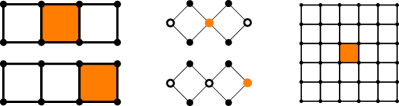
Figure 5: In the left column we show two clusters which would be obtained by starting the search process on the lattice in the right column from the orange bond (plaquette). In the central column the reduced König representations are shown. The orange vertices indicate the position of the first vertex for the two isomorphic graphs. When enforcing the canonical location of the first vertex, only one of the subclusters has to be considered. If one chooses the first subcluster, then the location of the first vertex in the graph is unique. In contrast, for the lower subcluster, there are two valid locations for the first vertex due to the reflection symmetry. This ambiguity has to be corrected by dividing the number of embeddings by 2. Our approach can therefore be seen as a bottom-up version of the embedding process described in Oitmaa et al. (2006), where an edge in the graph is fixed to a bond in the lattice during the embedding process.

IV.1.3 Putting the pieces together

The vacuum energy is an extensive quantity so we aim to calculate the vacuum energy per plaquette. As a starting point we recall from Sec. III.1 that we could find all connected subclusters up to a given number of bonds which include a given starting bond. For further explanations the vertex representing the starting bond will be referred to as the first vertex. In order to find the number of subclusters per plaquette, the first vertex must always have a canonical location in the subclusters. If this requirement is not fulfilled on a subcluster, it is not counted as a valid embedding. Enforcing the canonical location of the first vertex corresponds to fixing an hyperedge of the respective hypergraph to a bond in the lattice similar to the description for conventional graphs in Oitmaa et al. (2006).

As this requirement is considered during isomorphism checking, we will continue with the sorting of the instances into isomorphism classes. To sort a subcluster into an isomorphism class, we use its reduced König representation as described in Sec. III.2. We first calculate a combination of heuristic graph invariants, and then perform isomorphism checks using the RI algorithm Bonnici et al. (2013); Bonnici and Giugno (2017) among the already discovered graphs with the same invariants. If no isomorphic graph is found, we discovered a new isomorphism class, which we insert into the list of isomorphism classes with an embedding count of one. If an isomorphic graph is found, we check whether there is an isomorphism which preserves the first vertex, i.e., it maps the first vertices of both graphs onto each other. If such an isomorphism exists we increase the embedding count of the respective equivalence class by one. If no such isomorphism exists, the current instance is associated with another bond and the embedding count is not increased. In this way, we define a canonical position for the first vertex for every isomorphism class which for example can be based on the first obtained representant. Whenever we accept a subcluster based on the previous criteria, we increase the embedding count by one. If the canonical position of the first vertex is ambiguous, i.e. the corresponding automorphism orbit contains multiple elements, we need to correct the final embedding number dividing it by the size of the respective orbit. In this way we find a list of subclusters and their embedding numbers and can proceed to the final evaluation of matrix elements, which can be done with the commonly employed approaches like bookkeeping techniques Coester and Schmidt (2015) or recursive subcluster subtraction schemes Gelfand and Singh (2000); Oitmaa et al. (2006).

IV.1.4 Vacuum energy series

We calculated the vacuum energy per plaquette for (17) up to order twelve

$$e_{0}= -\frac{1}{3}-\frac{{{\lambda}^{2}}}{8}-\frac{113{{\lambda}^{4}}}{1536}-\frac{21427{{\lambda}^{6}}}{163840}-\frac{87959384893{{\lambda}^{8}}}{254803968000}$$ (19)

$$-\frac{115181804621864639{{\lambda}^{10}}}{102736959897600000}$$

$$-\frac{1199864820008961969940451{{\lambda}^{12}}}{289964795614986240000000}\,,$$

using Löwdin’s partitioning technique Löwdin (1962); Kalis et al. (2012) with a bookkeeping technique Coester and Schmidt (2015) for the evaluation. After proper rearrangements this agrees with the available result in order six obtained in Mühlhauser et al. (2020). We have therefore significantly extended the maximal order of the vacuum energy series with our hypergraph approach.

IV.2 Hopping elements

The calculation of hopping elements is quite analogue to the previously described calculation of the vacuum energy. The main difference is that we now need all subclusters which contain at least one site which is occupied, i.e., different from the local vacuum, in the initial state. Furthermore any considered cluster should contain all sites, which change their local state in the matrix element of interest. Accordingly, we start the search process several times, from all the bonds containing any of the sites which are occupied in the initial state. Obviously, when we restart the search from a different bond, all the previous starting bonds are ignored in order to avoid duplicates as described in Rücker and Rücker (2000).

We also have to slightly modify the employed equivalence relation, as the equivalence of subclusters now depends crucially on the states involved in the matrix element. To this end we distinguish the vertices based on the associated local states. In our case it is sufficient to distinguish between four possibilities, namely occupied in the initial state, occupied in the final state, both or none of the two. As a consequence, we have to slightly tweak the reduced representation which we used for the vacuum energy. This can be achieved by keeping the vertices of degree one which correspond to sites occupied in the final state, in the initial state, or in both states. In this setting simply testing for isomorphism is sufficient, and we do not need the first vertex to be in a canonical location as for the vacuum energy. The embedding counts of the isomorphism classes are simply given by the number of subclusters which belong to the given class.

Also the heuristics to discard non-contributing clusters or equivalence classes have to be adapted. This can be done by assuming that only sites which are unoccupied in the initial and final state require to be modified an even number of times by the perturbation. Depending on which technique is employed only these sites or vertices have to be counted or covered. For the problem at hand we can also require that sites which remain occupied have to be affected an even number of times by the perturbation, and sites which change their occupation number are touched an odd number of times. In addition we can employ another check, which determines whether all sites which have to be on the subcluster can be reached by expanding the subcluster up to a given number of bonds. If this is not the case the subcluster is not further expanded and discarded. The distances from the relevant sites can be calculated once before the actual search processes start.

To give an exemplary result we calculated the gap of two adjacent spin-flip excitations for the transverse field plaquette Ising model (17), as this is the energetically lowest mobile excitation Shirley et al. (2019); Mühlhauser et al. (2020). Observing that the parity of the excitation number in each plane is conserved, one sees that single spin-flip excitations are immobile Vijay et al. (2016), and the described two spin-flip excitations stay together as nearest neighbours with fixed orientation and can only move within a plane Slagle and Kim (2018). As a consequence, this particle sector can be diagonalized using Fourier transformation. The gap $\Delta_{2}$ of the resulting dispersion is located at $\vec{k}=0$ and reads

$$\Delta_{2}= 4-4\lambda-3{{\lambda}^{2}}-\frac{17{{\lambda}^{3}}}{8}-\frac{1151{{\lambda}^{4}}}{192}-\frac{37165{{\lambda}^{5}}}{9216}$$ (20)

$$-\frac{2591423{{\lambda}^{6}}}{122880}-\frac{6264944713{{\lambda}^{7}}}{530841600}$$

$$-\frac{5707377242657{{\lambda}^{8}}}{63700992000}-\frac{2114517232207{{\lambda}^{9}}}{53084160000}$$

$$-\frac{2169534326790862117{{\lambda}^{10}}}{5136847994880000}\,,$$

which coincides with the series up to order seven obtained in Mühlhauser et al. (2020). Here we evaluated the contributions of the subclusters using pCUT with a bookkeeping technique Coester and Schmidt (2015). Again, our approach provides a significant extension of the maximal order (see also App. C).

V Conclusion

In this work we presented a straightforward and relatively general approach to incorporate effective many-site interactions into graph decompositions. Although the involved methods and theoretical foundations are well established, we believe that the presented combination of all this to a general approach for multi-site interactions is valuable for perturbative linked cluster expansions of quantum many-body systems.

It is clear that the presented scheme cannot compete with the well established graph decomposition techniques Gelfand and Singh (2000); Oitmaa et al. (2006) where they are applicable. One of the reasons is the large overhead of the internal representation of hypergraphs and related information. Furthermore, our approach to identify non-contributing clusters can still be improved by using more efficient algorithms for subtasks, like the partitioning of the set of odd-degree vertices into bonds, but also by conceptional improvements of the heuristics themselves.

As quantum many-body systems containing multi-site interactions play an important role in current research due to their exotic physical properties like topological or fracton order, we are strongly convinced that the presented approach can be successfully used in various systems in the future. It would be further interesting to use the described hypergraph approach with non-perturbative numerical linked cluster expansions.

Appendix A More general settings

In this appendix we discuss relatively common generalizations and propose solutions. The first generalization is the presence of several bond types. While for the plaquette Ising model in a transverse field (17) we were able to directly calculate the vacuum energy per plaquette, the presence of different bond types requires some further considerations. Obviously, the graph representation is modified taking into account the bond type as a vertex label assigned to the vertices in the edge-partition, which should at the same time still be distinguishable from the vertices in the vertex-partition. For the vacuum energy one has to be careful ensuring the right embedding counts. One possibility is to define some sort of unit cell, where all bond types are contained and which is periodically repeated. If all bond types in this unit cell are different, we can simply start the search process from every bond type ignoring the bond types of the former starting bonds, as all relevant subclusters involving former starting bonds have already been discovered. In principle if some bond type appears multiple times in such a unit cell, one can just distinguish bond types arbitrarily. For the calculations of the hopping elements we do not expect such complications, and thus assigning additional vertex labels for the edge-partition should suffice.

The treatment of more than two local states should only require modifications for the calculation of hopping elements, as more local states have to be distinguished.

To treat directed interactions, where the local interaction matrix elements depend on the specific sites within a bond, we propose to use an edge-colored version of the reduced König representation in order to distinguish the different sites in the bond. Actually, this can be interpreted as the representation of a sequence hypergraph, i.e. a hypergraph where the hyperedges are given by sequences instead of sets Böhmová et al. (2016). Although they can be seen as a generalization of directed graphs, they are not to be confused with directed hypergraphs Böhmová et al. (2016); Gallo et al. (1993); Bretto (2013)

Appendix B Truncating the search tree using graph coloring

In this appendix we aim to give a simple example for the transitive heuristic to discard non-contributing clusters for which we use graph coloring. To this end we consider a calculation of the ground-state energy of the well known transverse field Ising model on a square lattice in the high-field limit

$$H^{\lambda\ll 1}_{\text{TFIM}}=-\sum_{i}\sigma_{i}^{z}-\lambda\sum_{\langle i,j\rangle}\sigma^{x}_{i}\sigma^{x}_{j}\qquad\lambda\ll 1\,.$$

We consider this example, because it allows us to keep images comprehensive and simple, and it is readily generalized to other suitable problems. In Fig. 6 we show the embeddings of two clusters which one encounters within the calculation of the vacuum energy and belong to the same isomorphism class. For both of these embeddings we go through four steps, which are represented by the rows in Fig. 6. The first step is to specify the actual realization of the cluster within the lattice. Then we identify the sites, which have odd-degree in each cluster. As described in Sec. IV.1.2 this information can already be used to discard non-contributing clusters Oitmaa et al. (2006). In the present case, the corresponding graph has 8 edges and 4 vertices of odd degree. As each bond covers 2 vertices, we can conclude, that at least two edges have to be added to get rid of the odd-degree vertices. Accordingly, this graph can contribute only in order ten or higher.

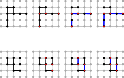
Figure 6: Considerations about two different clusters (upper/lower row) which belong to the same isomorphism class. From left to right: We first give the position of the cluster in the actual lattice. Then in the next column we mark all vertices of odd-degree red. In the third column we mark a minimum set of bonds, such that all odd-degree vertices are covered. To show that this is again only an estimate, we consider coverings, where all vertices in the cluster will have even degree after addition (duplication) of the blue edges.

In an actual calculation we can store the adjacency information of all the sites in the lattice, i.e. we store whether two sites share a common bond. We can use this information to find a lower bound to the number of bonds which are needed in order to cover the sites of odd degree. Obviously, two sites, which do not share a bond, cannot be covered by the same bond. So we search for a partition of the odd-degree sites, such that non-adjacent sites are in different parts. A lower bound to the number of parts is actually given by the chromatic number. The chromatic number of a graph is the minimum number of colors necessary to find a feasible coloring, i.e. a coloring which assigns a color to every vertex of the graph, such that adjacent vertices never have the same color Lewis (2016). The chromatic number is calculated for the graph where vertices represent odd-degree sites and pairs of vertices are joined by an edge, whenever they do not share a bond. It is intuitively clear that pairs of vertices, which do not share a bond, will be assigned different colors. And thus the coloring provides exactly the partition we searched for.

Figure 7: The graphs which have to be colored to check the two clusters in Fig. 6. Due to the different embeddings in the lattice of the corresponding clusters the upper graph has a higher chromatic number, and thus we need more bonds to cover the odd-degree sites.

Note that using graph coloring, to solve these kinds of problems is a standard technique Lewis (2016). Of course, when checking if we can discard a cluster and its descendants we do not need to know the chromatic number. We just need to know whether it exceeds the number of bonds which can be appended down the search tree. So instead of computing the chromatic number, we check if it is possible to find a feasible coloring with $r$ colors, where $r=(O_{\text{pert}}-N_{\text{bonds}})$. This can be decided with a simple backtracking algorithm. As this decision is even simpler for $r=1,2$ specialized solutions for these cases should be considered for optimization. We also see that these heuristics can still be improved, as duplicating the three blue bonds on the cluster in the upper row of Fig. 6 does create new odd-degree sites.

In the fourth step, we provide a set of bonds which does not leave any odd-degree sites, in order to show, that there is still a lot of space for improvement in the pruning of the search tree for these kinds of models.

Appendix C Comparison to calculations on single clusters

In order to estimate the benefit of the presented linked cluster expansions compared to calculations on sufficiently large clusters in the context of the examples given in Sec. IV, we performed two explicit calculations collecting some information about CPU-time and memory usage with the help of GNU time.

First we determined the vacuum energy per plaquette up to order 6 evaluating the effective pCUT-Hamiltonian on a periodic cluster of $7\times 7\times 7$ spins. This calculation took more than 30 minutes of CPU time, and over 30 GB of maximum resident set size (RSS). Instead, with the described method we obtained equivalent results in less than 1 s of CPU-time and a maximum RSS below 5 MB on the same system. Furthermore, we calculated the matrix element of two adjacent spin excitations hopping by one site on a cluster with $8\times 8\times 7$ spins. The calculation took more than 25 hours of CPU time and a maximal RSS of around 70 GB, while with the presented method it took less than 4 minutes of CPU time and a maximal RSS of less than 15 MB to obtain the same result. For both of these calculations pCUT with a bookkeeping technique Coester and Schmidt (2015) was used for evaluation.

References

- Marland (1981) L. G. Marland, Journal of Physics A: Mathematical and General 14, 2047 (1981).
- Irving and Hamer (1984) A. Irving and C. Hamer, Nuclear Physics B 230, 361 (1984).
- He et al. (1990) H. X. He, C. J. Hamer, and J. Oitmaa, Journal of Physics A: Mathematical and General 23, 1775 (1990).
- Oitmaa et al. (1991) J. Oitmaa, C. J. Hamer, and Z. Weihong, Journal of Physics A: Mathematical and General 24, 2863 (1991).
- Hamer et al. (1992) C. J. Hamer, J. Oitmaa, and Z. Weihong, Journal of Physics A: Mathematical and General 25, 1821 (1992).
- Hehn et al. (2017) A. Hehn, N. van Well, and M. Troyer, Computer Physics Communications 212, 180–188 (2017).
- Singh and Oitmaa (2017) R. R. P. Singh and J. Oitmaa, Phys. Rev. B 96, 144414 (2017).
- Hehn (2016) A. R. Hehn, Series expansion methods for quantum lattice models, Ph.D. thesis, ETH Zurich (2016).
- Oitmaa (2020) J. Oitmaa, Journal of Physics A: Mathematical and Theoretical 53, 085001 (2020).
- Oitmaa (2021) J. Oitmaa, Phys. Rev. B 103, 214446 (2021).
- Knetter and Uhrig (2000) C. Knetter and G. Uhrig, The European Physical Journal B 13, 209–225 (2000).
- Knetter et al. (2003) C. Knetter, K. P. Schmidt, and G. S. Uhrig, Journal of Physics A: Mathematical and General 36, 7889 (2003).
- Yang et al. (2010a) H.-Y. Yang, A. M. Läuchli, F. Mila, and K. P. Schmidt, Phys. Rev. Lett. 105, 267204 (2010a).
- Coester et al. (2016) K. Coester, D. G. Joshi, M. Vojta, and K. P. Schmidt, Physical Review B 94, 125109 (2016).
- Adelhardt et al. (2020) P. Adelhardt, J. A. Koziol, A. Schellenberger, and K. P. Schmidt, Phys. Rev. B 102, 174424 (2020).
- Schmoll et al. (2020) P. Schmoll, S. S. Jahromi, M. Hörmann, M. Mühlhauser, K. P. Schmidt, and R. Orús, Physical Review Letters 124, 200603 (2020).
- Ixert and Schmidt (2016) D. Ixert and K. P. Schmidt, Phys. Rev. B 94, 195133 (2016).
- Rigol et al. (2006) M. Rigol, T. Bryant, and R. R. P. Singh, Physical Review Letters 97, 187202 (2006).
- Schäfer et al. (2020) R. Schäfer, I. Hagymási, R. Moessner, and D. J. Luitz, Physical Review B 102, 054408 (2020).
- Stoudenmire et al. (2014) E. M. Stoudenmire, P. Gustainis, R. Johal, S. Wessel, and R. G. Melko, Phys. Rev. B 90, 235106 (2014).
- Yang and Schmidt (2011) H. Y. Yang and K. P. Schmidt, EPL (Europhysics Letters) 94, 17004 (2011).
- Ixert et al. (2014) D. Ixert, F. F. Assaad, and K. P. Schmidt, Phys. Rev. B 90, 195133 (2014).
- Coester et al. (2015) K. Coester, S. Clever, F. Herbst, S. Capponi, and K. P. Schmidt, EPL (Europhysics Letters) 110, 20006 (2015).
- Gelfand (1996) M. P. Gelfand, Solid State Communications 98, 11–14 (1996).
- Trebst et al. (2000) S. Trebst, H. Monien, C. J. Hamer, Z. Weihong, and R. R. P. Singh, Physical Review Letters 85, 4373–4376 (2000).
- Zheng et al. (2001) W. Zheng, C. J. Hamer, R. R. P. Singh, S. Trebst, and H. Monien, Physical Review B 63, 144410 (2001).
- Knetter et al. (2000) C. Knetter, A. Bühler, E. Müller-Hartmann, and G. S. Uhrig, Phys. Rev. Lett. 85, 3958 (2000).
- Schmidt et al. (2001) K. P. Schmidt, C. Knetter, and G. S. Uhrig, Europhysics Letters (EPL) 56, 877 (2001).
- Knetter et al. (2001) C. Knetter, K. P. Schmidt, M. Grüninger, and G. S. Uhrig, Phys. Rev. Lett. 87, 167204 (2001).
- Hörmann et al. (2018) M. Hörmann, P. Wunderlich, and K. P. Schmidt, Phys. Rev. Lett. 121, 167201 (2018).
- Gelfand and Singh (2000) M. P. Gelfand and R. R. P. Singh, Advances in Physics 49, 93 (2000).
- Oitmaa et al. (2006) J. Oitmaa, C. Hamer, and W. Zheng, Series Expansion Methods for Strongly Interacting Lattice Models (Cambridge University Press, 2006).
- Joshi et al. (2015) D. G. Joshi, K. Coester, K. P. Schmidt, and M. Vojta, Phys. Rev. B 91, 094404 (2015).
- Schulz et al. (2013) M. D. Schulz, S. Dusuel, K. P. Schmidt, and J. Vidal, Phys. Rev. Lett. 110, 147203 (2013).
- Schulz et al. (2014) M. D. Schulz, S. Dusuel, G. Misguich, K. P. Schmidt, and J. Vidal, Phys. Rev. B 89, 201103 (2014).
- Baxter and Wu (1973) R. J. Baxter and F. Y. Wu, Phys. Rev. Lett. 31, 1294 (1973).
- Capponi et al. (2014) S. Capponi, S. S. Jahromi, F. Alet, and K. P. Schmidt, Phys. Rev. E 89, 062136 (2014).
- Zhou et al. (2021) Z. Zhou, X.-F. Zhang, F. Pollmann, and Y. You, “Fractal quantum phase transitions: Critical phenomena beyond renormalization,” (2021), arXiv:2105.05851 [cond-mat.str-el] .
- Gottesman (1997) D. Gottesman, “Stabilizer codes and quantum error correction,” (1997), arXiv:quant-ph/9705052 [quant-ph] .
- Kitaev (2003) A. Kitaev, Annals of Physics 303, 2 (2003).
- Hamma et al. (2005) A. Hamma, P. Zanardi, and X.-G. Wen, Physical Review B 72, 035307 (2005).
- Nussinov and Ortiz (2008) Z. Nussinov and G. Ortiz, Physical Review B 77, 064302 (2008).
- Reiss and Schmidt (2019) D. A. Reiss and K. P. Schmidt, SciPost Phys. 6, 78 (2019).
- Kargarian (2009) M. Kargarian, Phys. Rev. A 80, 012321 (2009).
- Katzgraber et al. (2009) H. G. Katzgraber, H. Bombin, and M. A. Martin-Delgado, Phys. Rev. Lett. 103, 090501 (2009).
- Levin and Wen (2005) M. A. Levin and X.-G. Wen, Phys. Rev. B 71, 045110 (2005).
- Haah (2011) J. Haah, Phys. Rev. A 83, 042330 (2011).
- Vijay et al. (2016) S. Vijay, J. Haah, and L. Fu, Phys. Rev. B 94, 235157 (2016).
- Raussendorf and Briegel (2001) R. Raussendorf and H. J. Briegel, Phys. Rev. Lett. 86, 5188 (2001).
- Briegel and Raussendorf (2001) H. J. Briegel and R. Raussendorf, Phys. Rev. Lett. 86, 910 (2001).
- Orús et al. (2013) R. Orús, H. Kalis, M. Bornemann, and K. P. Schmidt, Phys. Rev. A 87, 062312 (2013).
- Dusuel et al. (2011) S. Dusuel, M. Kamfor, R. Orús, K. P. Schmidt, and J. Vidal, Phys. Rev. Lett. 106, 107203 (2011).
- Kalis et al. (2012) H. Kalis, D. Klagges, R. Orús, and K. P. Schmidt, Phys. Rev. A 86, 022317 (2012).
- Jahromi et al. (2013) S. S. Jahromi, M. Kargarian, S. F. Masoudi, and K. P. Schmidt, Phys. Rev. B 87, 094413 (2013).
- Mühlhauser et al. (2020) M. Mühlhauser, M. R. Walther, D. A. Reiss, and K. P. Schmidt, Physical Review B 101, 054426 (2020).
- MacDonald et al. (1988) A. H. MacDonald, S. M. Girvin, and D. Yoshioka, Phys. Rev. B 37, 9753 (1988).
- Reischl et al. (2004) A. Reischl, E. Müller-Hartmann, and G. S. Uhrig, Phys. Rev. B 70, 245124 (2004).
- Yang et al. (2010b) H.-Y. Yang, A. M. Läuchli, F. Mila, and K. P. Schmidt, Phys. Rev. Lett. 105, 267204 (2010b).
- Yang et al. (2012) H.-Y. Yang, A. F. Albuquerque, S. Capponi, A. M. Läuchli, and K. P. Schmidt, New Journal of Physics 14, 115027 (2012).
- Windt et al. (2001) M. Windt, M. Grüninger, T. Nunner, C. Knetter, K. P. Schmidt, G. S. Uhrig, T. Kopp, A. Freimuth, U. Ammerahl, B. Büchner, and A. Revcolevschi, Phys. Rev. Lett. 87, 127002 (2001).
- Katanin and Kampf (2003) A. A. Katanin and A. P. Kampf, Phys. Rev. B 67, 100404 (2003).
- Schmidt et al. (2005) K. P. Schmidt, A. Gössling, U. Kuhlmann, C. Thomsen, A. Löffert, C. Gross, and W. Assmus, Phys. Rev. B 72, 094419 (2005).
- Schmidt and Uhrig (2005) K. P. Schmidt and G. S. Uhrig, Modern Physics Letters B 19, 1179 (2005).
- Notbohm et al. (2007) S. Notbohm, P. Ribeiro, B. Lake, D. A. Tennant, K. P. Schmidt, G. S. Uhrig, C. Hess, R. Klingeler, G. Behr, B. Büchner, M. Reehuis, R. I. Bewley, C. D. Frost, P. Manuel, and R. S. Eccleston, Phys. Rev. Lett. 98, 027403 (2007).
- Motrunich (2005) O. I. Motrunich, Phys. Rev. B 72, 045105 (2005).
- Sheng et al. (2009) D. N. Sheng, O. I. Motrunich, and M. P. A. Fisher, Phys. Rev. B 79, 205112 (2009).
- Block et al. (2011) M. S. Block, D. N. Sheng, O. I. Motrunich, and M. P. A. Fisher, Phys. Rev. Lett. 106, 157202 (2011).
- Boos et al. (2020) C. Boos, C. J. Ganahl, M. Lajkó, P. Nataf, A. M. Läuchli, K. Penc, K. P. Schmidt, and F. Mila, Phys. Rev. Research 2, 023098 (2020).
- Szasz et al. (2020) A. Szasz, J. Motruk, M. P. Zaletel, and J. E. Moore, Phys. Rev. X 10, 021042 (2020).
- Berge (1973) C. Berge, Graphs and Hypergraphs (North-Holland, 1973).
- Zykov (1974) A. A. Zykov, Russian Mathematical Surveys 29, 89 (1974).
- Berge (1989) C. Berge, Hypergraphs (North-Holland, 1989).
- Bretto (2013) A. Bretto, Hypergraph Theory (Springer, 2013).
- Ouvrard (2020) X. Ouvrard, “Hypergraphs: an introduction and review,” (2020), arXiv:2002.05014 .
- Konstantinova and Skorobogatov (1995) E. V. Konstantinova and V. A. Skorobogatov, Journal of Chemical Information and Computer Sciences 35, 472 (1995).
- Konstantinova and Skorobogatov (2001) E. V. Konstantinova and V. A. Skorobogatov, Discrete Mathematics 235, 365 (2001).
- McKay (1981) B. D. McKay, Congressus Numerantium 30, 45 (1981).
- Mühlhauser et al. (2021) M. Mühlhauser, K. P. Schmidt, J. Vidal, and M. R. Walther, “Competing topological orders in three dimensions,” (2021), arXiv:2106.05749 [cond-mat.str-el] .
- Savvidy et al. (1995) G. Savvidy, K. Savvidy, and F. Wegner, Nuclear Physics B 443, 565 (1995).
- Johnston et al. (2017) D. A. Johnston, M. Mueller, and W. Janke, The European Physical Journal Special Topics 226, 749 (2017).
- Nandkishore and Hermele (2019) R. M. Nandkishore and M. Hermele, Annual Review of Condensed Matter Physics 10, 295 (2019).
- Coester and Schmidt (2015) K. Coester and K. P. Schmidt, Physical Review E 92, 022118 (2015).
- Dusuel et al. (2010) S. Dusuel, M. Kamfor, K. P. Schmidt, R. Thomale, and J. Vidal, Physical Review B 81 (2010), 10.1103/physrevb.81.064412.
- Kamfor (2013) M. Kamfor, Robustness and spectroscopy of the toric code in a magnetic field, Ph.D. thesis, Technische Universität Dortmund (2013).
- Takahashi (1977) M. Takahashi, Journal of Physics C: Solid State Physics 10, 1289 (1977).
- Klagges and Schmidt (2012) D. Klagges and K. P. Schmidt, Phys. Rev. Lett. 108, 230508 (2012).
- Löwdin (1962) P.-O. Löwdin, J. Math. Phys. 3, 969 (1962).
- McKay (1998) B. D. McKay, Journal of Algorithms 26, 306 (1998).
- Rücker and Rücker (2000) G. Rücker and C. Rücker, MATCH Commun. Math. Comput. Chem. 41, 145 (2000).
- Rücker and Rücker (2001) G. Rücker and C. Rücker, Journal of Chemical Information and Computer Sciences 41, 314 (2001).
- Rücker et al. (2002) C. Rücker, G. Rücker, and M. Meringer, Journal of Chemical Information and Computer Sciences 42, 640 (2002).
- Note (1) Remarkably, an illustration in Ref. Schulz2013phd is actually showing a König graph, but then a different slightly more problem specific approach is used to distinguish equivalence classes of clusters.
- Bonnici et al. (2013) V. Bonnici, R. Giugno, A. Pulvirenti, D. Shasha, and A. Ferro, BMC Bioinformatics 14, S13 (2013).
- Bonnici and Giugno (2017) V. Bonnici and R. Giugno, IEEE/ACM Transactions on Computational Biology and Bioinformatics 14, 193 (2017).
- Savvidy and Wegner (1994) G. Savvidy and F. Wegner, Nuclear Physics B 413, 605 (1994).
- Devakul et al. (2018) T. Devakul, S. A. Parameswaran, and S. L. Sondhi, Phys. Rev. B 97, 041110 (2018).
- Coester (2011) K. Coester, Series expansions for dimerized quantum spin systems, Diploma thesis, Technische Universität Dortmund (2011).
- Lewis (2016) R. Lewis, A Guide to Graph Colouring (Springer International Publishing, 2016).
- Shirley et al. (2019) W. Shirley, K. Slagle, and X. Chen, Annals of Physics 410, 167922 (2019).
- Slagle and Kim (2018) K. Slagle and Y. B. Kim, Phys. Rev. B 97, 165106 (2018).
- Böhmová et al. (2016) K. Böhmová, J. Chalopin, M. Mihalák, G. Proietti, and P. Widmayer, in Graph-Theoretic Concepts in Computer Science, edited by P. Heggernes (Springer, 2016) pp. 282–294.
- Gallo et al. (1993) G. Gallo, G. Longo, S. Pallottino, and S. Nguyen, Discrete Applied Mathematics 42, 177 (1993).