Efficient Direct-Connect Topologies for Collective Communications

Abstract

We consider the problem of distilling efficient network topologies for collective communications. We provide an algorithmic framework for constructing direct-connect topologies optimized for the latency vs. bandwidth trade-off associated with the workload. Our approach synthesizes many different topologies and schedules for a given cluster size and degree and then identifies the appropriate topology and schedule for a given workload. Our algorithms start from small, optimal base topologies and associated communication schedules and use a set of techniques that can be iteratively applied to derive much larger topologies and schedules. Additionally, we incorporate well-studied large-scale graph topologies into our algorithmic framework by producing efficient collective schedules for them using a novel polynomial-time algorithm. Our evaluation uses multiple testbeds and large-scale simulations to demonstrate significant performance benefits from our derived topologies and schedules.

1 Introduction

Collective communication operations involve concurrently aggregating and distributing data on a cluster of nodes and are used in both machine learning (ML) and high-performance computing (HPC). With the explosive growth in model sizes and improved computational capabilities, collective operations are a significant overhead in large-scale distributed ML training [59, 29, 70].

An emerging approach to meet these challenging demands has been to employ various forms of optical circuit switching to achieve higher bandwidths at reasonable capital expenditure and energy costs [38, 71, 75, 45, 67, 37, 44]. Hosts communicate using a limited number of optical circuits that can be reconfigured at timescales appropriate for the hardware (see §2.1), thus exposing network topology as a configurable component. We refer to this setting as direct-connect with circuits that are configured and fixed for an appropriate duration.

Existing optical-circuits-based ML systems [38, 75, 45, 67] fit this direct-connect model but are unable to exploit the flexibility offered by topology reconfiguration. They are constrained to choose from a few well-known collective algorithms whose communication patterns can be realized within the constraints of the optical fabric (e.g., rings, multi-rings, tori, and trees with bounded degree) and accept the consequent performance tradeoffs. For example, collective communications over a ring, while bandwidth-efficient, have high latency as messages must travel around the ring, and a double binary tree has logarithmic latency but suffers from load imbalances and bandwidth inefficiencies. Conversely, the broader spectrum of well-known collective algorithms that achieve desired latency and bandwidth (e.g., recursive-doubling, Bruck algorithm) [66, 72] use dynamic communication patterns ideal for switch networks but are ill-suited for direct-connect networks.

To fill this gap, we seek to identify new topologies and communication schedules that are custom-built for direct-connect networks. We pose the following research question: How to efficiently construct high-performance direct-connect topologies and communication schedules for a collectives workload given the network’s performance characteristics and degree constraints?

Several challenges need to be tackled in addressing this question. First, jointly optimizing both the network topology and the corresponding communication schedule is intractable at a large scale. Prior efforts reduce the search complexity by optimizing only one or the other (e.g., schedules for a given network [70, 19, 60] or topology permutations while retaining a ring schedule [71]). The combination of topological structure and communication schedule as degrees of freedom explodes the search space at a large scale, making this a seemingly intractable problem. Second, the optimization needs to carefully consider the workloads and performance characteristics of the network fabric. For example, minimizing the diameter of the topology and the number of hops in the communication schedule is ideal for small data sizes, while minimizing imbalance in communication load across links is critical for bandwidth-sensitive larger data sizes. Finding a single topology and schedule optimal for all workloads and fabrics is difficult and might be impossible in most cases. Finally, lowering the synthesized schedules to the underlying hardware and runtimes [34, 49, 3] in an efficient way requires careful scheduling to achieve the desired performance.

Our work addresses these issues by developing an algorithmic toolchain for quickly synthesizing efficient topologies and schedules for collective communications. We make the following contributions to achieve this goal:

1. We devise a range of expansion techniques for synthesizing custom large-scale network topologies and schedules. The expansions start with small, optimal topologies and communication schedules and expand them to achieve near-optimal large-scale topologies and schedules.

2. We devise a polynomial-time schedule generation algorithm to produce optimal collective communication schedules for large-scale topologies with certain symmetry properties. Consequently, our framework can also leverage existing well-studied topologies for collective communication.

3. We devise a topology enumeration and search algorithm to identify the best option for a target cluster and workload by exploring the Pareto-efficient options that provide different trade-offs for bandwidth and latency.

4. We develop compilers to realize our optimized schedules. We offer efficient implementations for both GPUs and CPUs, and integrate with ML frameworks (e.g. PyTorch) through the MSCCL [49] and oneCCL [3] runtimes.

We evaluate our approach using two testbeds: a 12-node GPU cluster capable of topology reconfiguration, and torus clusters on Frontera [64] supercomputer with up to 54 CPU nodes. Our techniques reduce collective communication latencies by $>\!30\%$ for DNN training on the GPU testbed, and upto $3.1\times$ for HPC workloads on the supercomputer. Simulations for large-scale DNN training show upto order of magnitude reduction in total collective communication latency from topology and schedule optimization. Our schedule generation algorithm is orders of magnitude faster than state-of-the-art (e.g., SCCL [19] and TACCL [60]), capable of producing schedules for topologies with thousands of nodes in a minute.

2 Background & Related Work

2.1 Network Fabric

Our work identifies topologies and schedules helpful for a broad range of settings, such as switchless physical circuits, patch-panel optical circuits, and optical circuit switches. While these options differ in cost and reconfigurability [71], they can all benefit from custom-built topologies and schedules for collectives.

Switchless physical circuits require the least amount of fabric hardware. However, the network topology must remain reasonably static for long periods, as the reconfiguration is manual. Patch-panel optical circuits provide a higher degree of reconfigurability by using a mechanical solution (e.g., robotic arms) to perform physical reconfigurations through a patch panel. The reconfigurations occur on the scale of seconds, but the patch panel itself can scale to a large number of duplex ports and is reasonably cheap (e.g., 1008 ports at $100 per port [65]). Both options can benefit from a carefully curated topology optimized for the workload, but they would require the topology to remain static for the duration of a job or training run given the reconfiguration costs.

Commercially available optical circuit switches (OCS) can perform reconfigurations in $\approx$10ms, are more expensive than patch panels, and scale to fewer ports [55, 20] (e.g., Polatis 3D-MEMS switch has 384 ports at $520 per port [55]). Though OCSes support faster reconfigurations, the delays are still too high to support the rewiring of the circuits during a typical collective operation. As a consequence, they cannot take advantage of algorithms designed for full-bisection switches, such as recursive halving/doubling [66, 72], that exploit high logical degree over time to provide both latency and bandwidth optimality properties. Thus, OCSes can also benefit from the custom-built and low-degree topologies synthesized by our approach.

All of these optical technologies allow for a shared cluster to be split into multiple subclusters for running separate jobs [37], so each job can be configured with its own topology. Further, unidirectional topologies are technically feasible on optical testbeds. The optical cable contains two fibers, one for each direction, and the fabric can link them to two distinct end-hosts, thus enabling unidirectional topologies at no additional hardware cost. Unidirectionality gives greater freedom in topology design and can enable lower-diameter networks.

Research prototypes such as RotorNet[48] and Sirius[12] with $\mu s$ to $ns$ reconfiguration latency, respectively, are based on demand-oblivious switch architectures that use 1-hop relays and Valiant load balancing (VLB). While demand obliviousness is valuable for generic workloads, ML collectives have structured communication patterns, and it would be ideal to realize them without incurring the overhead of a VLB relay.

Evaluation target: In this paper, we use a reconfigurable optical patch panel to configure and evaluate different topologies. Given the high reconfiguration costs for the patch panel, we identify an efficient topology that will remain static for the duration of a job. Nevertheless, our techniques could be used to derive topologies for finer reconfiguration timescales if the hardware can efficiently support them.

2.2 Related Work

Several existing optical-circuit-based ML systems [38, 75, 45, 67, 71] fit the direct-connect model; however, they rely on existing implementations of collectives and choose ones appropriate for their hardware. Typically, communication libraries for ML training [59, 5, 29, 53] offer either ring collective for high-latency bandwidth-optimal transfers or tree collective, which has low latency but suffers from load-imbalances across links. Other topologies such as mesh, tori, hypercubes, etc., have also been explored in HPC systems [18, 30, 14, 54, 21, 22, 28], but their bandwidth-latency tradeoff choices are limited as well. Bandwidth and latency optimal collectives for switch networks such as recursive-doubling, Bruck algorithm [72, 66], BlueConnect [23], etc., are unsuitable for direct-connect networks, because their one-to-one communication patterns fail to utilize all available links, and they assume a fully connected network.

Our work uniquely considers joint optimization of both the network topology and the corresponding collective communication schedule at a large scale, while prior work either optimizes one or the other. For instance, TopoOpt [71] generates customized shifted-ring topologies to optimize concurrent collective and non-collective communications for hybrid data-parallel [43, 42, 26] and model-parallel [61, 52, 36] DNN training, respectively. The collective communications in TopoOpt still use existing ring collectives. Consequently, when data-parallel jobs dominate the workload, TopoOpt’s performance suffers from similar latency issues present in existing ring collectives (see §8.3). Our effort is complementary as it synthesizes new topologies and schedules for data-parallel collectives, but we do not optimize hybrid-parallel communications. Extending our work to jointly optimize topologies and schedules for hybrid parallelism is future work.

Recent work like Blink [70], SCCL [19], and TACCL [60] also focus on generating a collective schedule for a given topology. However, they all involve NP-hard optimizations that severely limit their scalability. SCCL is capable of generating optimal schedules, but it fails to generate a schedule in a reasonable time when the topology size is beyond 30 nodes. TACCL improves the scalability of SCCL by using communication sketches and also handles switch networks, but it sacrifices schedule performance and is still limited in scalability (see §8.5). In our approach, we either synthesize the schedule along with the topology or rely on a polynomial-time schedule generation technique that is provably optimal for networks with certain symmetry properties.

Generic large-scale topologies are typically not optimized for collective communication operations but for general datacenter networks [63, 69, 39, 16, 40, 73]. Some cannot be realized on direct-connect networks due to their high degree requirements [39, 16, 40, 73]. Any regular topologies suitable for collective communications can also be incorporated into our framework. For instance, we include several classical low-diameter expander graphs [56, 33] in our algorithmic framework.

3 Formal Model of Collective Communications

$M$	total data size	$\alpha$	node latency of one comm step
$N$	number of nodes	$B$	total egress bandwidth of a node
$S$	data shard ($|S|=\frac{M}{N}$)	$B/d$	bandwidth of a single link
$C$	data chunk ($C\subseteq S$)	$T_{L}(A)$	node latency of schedule
$d$	degree of topology	$T_{B}(A)$	bandwidth runtime of schedule
$V_{G}$	vertex/node set of $G$	$T^{*}_{L}\!(\!N\!,\!d)$	Moore optimality (Def 12)
$E_{G}$	edge/link set of $G$	$T^{*}_{B}(N)$	bandwidth optimality $\frac{M}{B}\cdot\frac{N-1}{N}$
$D(\!G\!)$	graph diameter of $G$	$N^{+}_{x}(u)$	nodes at distance $x$ from $u$
Table 9 for graph symbols		$N^{-}_{x}(u)$	nodes at distance $x$ to $u$

Table 1: Summary of Important Notations

Before	After
Reduce-Scatter
Node 0 Node 1 Node 2 $S_{0}^{(0)}$ $S_{0}^{(1)}$ $S_{0}^{(2)}$ $S_{1}^{(0)}$ $S_{1}^{(1)}$ $S_{1}^{(2)}$ $S_{2}^{(0)}$ $S_{2}^{(1)}$ $S_{2}^{(2)}$	Node 0 Node 1 Node 2 $\bigoplus_{i}S_{0}^{(i)}$ $\bigoplus_{i}S_{1}^{(i)}$ $\bigoplus_{i}S_{2}^{(i)}$
Allgather
Node 0 Node 1 Node 2 $S_{0}^{(0)}$ $S_{1}^{(1)}$ $S_{2}^{(2)}$	Node 0 Node 1 Node 2 $S_{0}^{(0)}$ $S_{0}^{(0)}$ $S_{0}^{(0)}$ $S_{1}^{(1)}$ $S_{1}^{(1)}$ $S_{1}^{(1)}$ $S_{2}^{(2)}$ $S_{2}^{(2)}$ $S_{2}^{(2)}$
Allreduce
Node 0 Node 1 Node 2 $S_{0}^{(0)}$ $S_{0}^{(1)}$ $S_{0}^{(2)}$ $S_{1}^{(0)}$ $S_{1}^{(1)}$ $S_{1}^{(2)}$ $S_{2}^{(0)}$ $S_{2}^{(1)}$ $S_{2}^{(2)}$	Node 0 Node 1 Node 2 $\bigoplus_{i}S_{0}^{(i)}$ $\bigoplus_{i}S_{0}^{(i)}$ $\bigoplus_{i}S_{0}^{(i)}$ $\bigoplus_{i}S_{1}^{(i)}$ $\bigoplus_{i}S_{1}^{(i)}$ $\bigoplus_{i}S_{1}^{(i)}$ $\bigoplus_{i}S_{2}^{(i)}$ $\bigoplus_{i}S_{2}^{(i)}$ $\bigoplus_{i}S_{2}^{(i)}$

Table 2: The state before and after the collective communications. $S_{j}^{(i)}$ denotes the $j$-th shard of data at node $i$ prior to the operation. In particular, the size of each $S_{j}^{(i)}$ is $|S_{j}^{(i)}|=M/N$. $\oplus$ is the reduction operator (e.g., sum).

We focus on three collective communication operations: reduce-scatter, allgather, and allreduce. In each operation, there are $N$ nodes operating on a vector of data of total size $M$. The data can be divided into $N$ shards. Table 2 shows an example of how three nodes perform all three collectives. In reduce-scatter, each node $i$ reduces the $i$-th shard from all other nodes; in allgather, each node $i$ broadcasts the $i$-th shard to all other nodes; in allreduce, each node $i$ ends up with the fully reduced vector of data.

Throughout the paper, we only elaborate on allgather schedule construction because the other two collectives are direct transformations. Since allgather and reduce-scatter are, respectively, simultaneous broadcasts and reductions for each node, we can construct reduce-scatter schedules in bidirectional topologies by simply reversing the communications in allgather schedules [21]. In unidirectional topologies, we utilize graph transposition to achieve a similar transformation (Appendix A). To construct a allreduce schedule, we concatenate reduce-scatter and allgather.

3.1 Communication Topology & Schedule

The network topology is modeled as a directed graph (digraph) $G=(V,E)$, where $V$ denotes the set of nodes ($|V|=N$) and $E$ denotes the set of directed links/edges. The direct-connect network imposes a constraint that all nodes have degree $d$, which is the number of connection ports on each host and is typically low and independent of $N$.

A communication algorithm $(G,A)$ uses the communication schedule $A$ on topology $G$. Schedule $A$ can be specified as what chunk $C$ is communicated over which link in which communication (comm) step $t$. We define chunk $C$ as a subset of shard $S$. Both $C$ and $S$ are specified as index sets of elements. Typically, $S$ is interval $[0,1]$ representing the whole shard, and $C$ is some subinterval. We denote $v$’s chunk $C$ as $(v,C)$, which is a subset of $v$’s shard $(v,S)$ (corresponding to $S_{v}^{(v)}$ in the allgather of Table 2). Let $((v,C),(u,w),t)$ denote that $v$’s chunk $C$ is sent by node $u$ to its neighbor $w$ at comm step $t$. Schedule $A$ then is specified as a list of tuples $((v,C),(u,w),t)$. Figure 1 gives an example of an allgather schedule in such a tuple notation. Within a schedule, chunks can be different-sized subsets of $S$. Appendix A gives formal definitions of reduce-scatter/allgather schedules.

3.2 Cost Model

We use the well-known $\alpha$-$\beta$ cost model [31]. The cost of sending a message of size $H$ over a link is $\alpha+\beta H$. This cost comprises two components: the constant latency $\alpha$ and a bandwidth component $\beta$, which is the inverse of link bandwidth, i.e., $\beta=\frac{1}{b}$. This simple model has been shown to be a good proxy for characterizing communication costs on existing GPU interconnects [41, 19, 60]. In our analysis, we use node bandwidth $B$ with $B=db$. In this paper, we focus on homogeneous networks, although some techniques also support heterogeneous ones (Appendix D.3).

The runtime of a schedule $A$ can be broken down into a node latency component and a bandwidth component. The node latency component $T_{L}(A)\!=\!t_{\max}\alpha$, where $t_{\max}$ is the number of comm steps. $T_{L}(A)$ represents the cost of performing schedule $A$ on an infinitesimal amount of data. The bandwidth component $T_{B}(A)$, or bandwidth (BW) runtime, is the sum of the BW runtime of each comm step, i.e., $\sum_{t}T_{B}(A_{t})$. The BW runtime of comm step $t$ is the max amount of data transmitted by a link within the comm step, divided by link bandwidth $b\!=\!B/d$. For $N$-node $d$-regular graphs, the optimal runtime of both reduce-scatter and allgather is approximately $\alpha\log_{d}N\!+\!\frac{1}{B}\!\cdot\!\frac{M(N-1)}{N}$. The 1st term represents the node latency required for communicating across the diameter of a topology, while the 2nd term represents the transmission time for any node to send/recv $N\!-\!1$ shards in reduce-scatter/allgather. One should not confuse node latency with overall latency, which is the sum of node latency and BW runtime. We omit the computational time of reduction and discuss this in §B.4.

We analyze the optimality of node latency and BW runtime separately. An algorithm $(G,A)$ is optimal in one component if no algorithm with the same $N,d$ can perform better. For BW runtime, an algorithm is bandwidth (BW) optimal iff its $T_{B}$ equals $T_{B}^{*}(N)\!\coloneqq\!\frac{M}{B}\!\cdot\!\frac{N-1}{N}$. For node latency, given $G$, the lowest $T_{L}$ achievable is $\alpha\!\cdot\!D(G)$, where $D(G)$ is the graph diameter of $G$. Thus, the optimal node latency equals the smallest diameter of any $N$-node $d$-regular graph. Computing this is still an open question in graph theory [50], so we define Moore optimality based on Moore bound, which provides a lower bound for diameter given $N,d$ and thus a well-defined $T_{L}^{*}(N,d)$. An algorithm is Moore optimal iff $T_{L}\!=\!T_{L}^{*}(N,d)$. Appendix B gives formal definitions of optimalities.

The ring allreduce [34] algorithm has a node latency that is linear in $N$, while the BW runtime is optimal. The double binary trees (DBT) algorithm [35], on the other hand, offers the advantage of logarithmic node latency but has suboptimal BW performance. Our work offers a range of topologies that are Pareto-efficient in node latency and BW performance.

4 Overview of Our Approach

We seek to jointly identify high-performance network topologies and communication schedules for collectives. At a small scale, one could hand pick one like a complete bipartite graph $K_{2,2}$ as a network topology at $N\!=\!4,d\!=\!2$. An allgather schedule that is both Moore and BW optimal could then be manually constructed as shown in Figure 1. However, how do we scale the topology and schedule generation to larger sizes? Our work approaches this problem with two tools: expansion techniques (§5) and BFB schedule generation (§6).

Figure 1: The allgather schedule of complete bipartite graph $K_{2,2}$. Shard $S$ is divided into two half chunks $C_{1}$ and $C_{2}$. From $a$, at the 1st comm step, $a$ sends the entire shard $S$ to both $c$ and $d$. At the 2nd comm step, $c$ and $d$ send the two half chunks $C_{1}$ and $C_{2}$ respectively to $b$. Thus, every node receives the full shard from $a$. By applying similar broadcast from $c,b,d$ in parallel, we have a complete BW-optimal allgather schedule with $T_{L}\!=\!2\alpha,T_{B}\!=\!\frac{M}{B}\!\cdot\!\frac{3}{4}$.

Expansion Techniques: Given a base topology and its communication schedule, expansion techniques enable us to expand it into a larger topology and associated schedule with minimal sacrifice in schedule performance. We call the resulting topologies synthesized topologies. The base topologies are small in scale, such as $K_{2,2}$ in Figure 1, for which straightforward schedules exist or an exhaustive search for the schedule is feasible. The line graph expansion can then expand $K_{2,2}$ and its schedule in Figure 1 to an allgather/reduce-scatter/allreduce algorithm with $N\!=\!4\!\cdot\!2^{n}$ for arbitrarily large $n$ while retaining a node degree of 2. Multiple expansion techniques can be composed to achieve the desired $N$ and $d$.

Breadth-First-Broadcast (BFB) Schedule Generation: Besides synthesized topologies, other large-scale topologies exist in graph theory (e.g., twisted torus, Generalized Kautz, and expander graphs). We call them generative topologies as they can be instantiated at various $N$ and $d$. The problem, though, is that efficient collective schedules are not known for many of these topologies, and existing schedule generators [19, 60] are intractable at moderate to large scale. Our work offers BFB schedule generation, a polynomial-time schedule generator that can generate high-performance schedules for large-scale topologies. For allgather, it performs a breadth-first broadcast from each node and uses linear programs to balance the workload on links. Although not always optimal, we show that BFB schedules are provably optimal for many topologies exhibiting certain graph symmetries. For instance, on any construction of torus, including those with unequal dimensions, we can generate a schedule with the lowest node latency and BW optimality.

With expansion techniques and BFB schedule generation, we can assemble a large pool of topologies and schedules, identify Pareto-efficient options from a node latency vs. BW performance perspective, and select from them for a given workload using our topology finder (§5.4). When two options are Pareto-efficient, one must be better than the other in either node latency or BW performance but not in both. Finally, the compiler (§7) lowers the chosen topology and schedule to the runtime and hardware.

(a) $K_{2,2}$ $(N\!=\!4,d\!=\!2)$

(b) $L(K_{2,2})$ $(N\!=\!8,d\!=\!2)$

(c) Broadcast from $ca$

Figure 2: The complete bipartite topology $K_{2,2}$ with its line graph $L(K_{2,2})$. Figure (a) shows the base topology and broadcast paths from $a$ to $c,b,d$ in $A_{K_{2,2}}$ (see figure 1). The number next to edge shows the comm step using the edge. Figure (b) shows the expanded topology. Observe that every edge in $K_{2,2}$ becomes a vertex in $L(K_{2,2})$, and two vertices are connected if the corresponding edges in $K_{2,2}$ have one’s head node being the other’s tail node. Figure (c) shows the broadcast paths of node $ca$, transformed from the broadcast paths of $a$ in figure (a). At the 1st comm step, by step 1 of def 2, $ca$ broadcasts its shard to all its neighbors: $((ca,S),(ca,ac),1)$, $((ca,S),(ca,ad),1)$. The rest of the broadcast paths are transformed from $A_{K_{2,2}}$ by step 2 of def 2, e.g. $((a,C_{1}),(c,b),2)\mapsto\{((ca,C_{1}),(cb,bc),3),((ca,C_{1}),(cb,bd),3)\}$. Each of the nodes $bc$ and $bd$ receives $C_{1},C_{2}$ from its two in-neighbors, just like $b$ does in $A_{K_{2,2}}$.

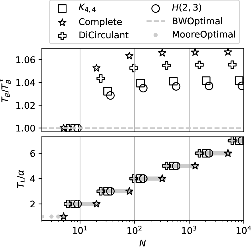
Figure 3: Line graph expansion on Moore and BW optimal degree-4 base graphs: complete bipartite graph $K_{4,4}$, complete graph, directed circulant graph, and Hamming graph $H(2,3)$. $T_{B}^{*}\!=\!\frac{M}{B}\!\cdot\!\frac{N-1}{N}$ is the optimal BW runtime.

5 Expansion Techniques

We present three techniques that can be applied to construct near-optimal large-scale synthesized topologies and schedules by iteratively expanding small-scale topologies and associated schedules. The three techniques provide different options for increasing the size of the topology and the per-node degree, while preserving either node latency or BW optimality of the base graph and schedule (Table 3). While we describe the techniques in the context of allgather, corollary 3.2 in §A implies equivalent constructions for reduce-scatter.

5.1 Line Graph Expansion

We borrow the following line graph transformation from graph theory, which transforms an input graph $G$ into a larger graph $L(G)$ that contains a vertex for every edge in $G$ and an edge for every pair of adjacent (directed) edges in $G$.

Definition 1 (Line Graph).

Given a directed graph (or digraph) $G$, each edge $(u,v)\in E_{G}$ corresponds to a vertex $uv$ in the line graph $L(G)$. For every $uv,vw$ pair in $V_{L(G)}$, there exists an edge $(uv,vw)\in E_{L(G)}$.

Figure 2(b) gives an example of the line graph of the complete bipartite graph $K_{2,2}$. There are two key properties for the line graph $L(G)$ of a $d$-regular topology $G$:

1. $L(G)$ has the same degree $d$ as $G$, while $|V_{L(G)}|=d|V_{G}|$;

2. If $w_{0}\!\!\mathrel{\vbox{\hbox{\rule[0.0pt]{4.0pt}{0.0pt}}}\mkern-4.0mu\hbox{\char 41\relax}}\!w_{1}\!\!\mathrel{\vbox{\hbox{\rule[0.0pt]{4.0pt}{0.0pt}}}\mkern-4.0mu\hbox{\char 41\relax}}\!\dots\!\!\mathrel{\vbox{\hbox{\rule[0.0pt]{4.0pt}{0.0pt}}}\mkern-4.0mu\hbox{\char 41\relax}}\!w_{n}$ is a (shortest) path in $G$, then $w_{-\!1}w_{0}\!\mathrel{\vbox{\hbox{\rule[0.0pt]{4.0pt}{0.0pt}}}\mkern-4.0mu\hbox{\char 41\relax}}\!w_{0}w_{1}\!\mathrel{\vbox{\hbox{\rule[0.0pt]{4.0pt}{0.0pt}}}\mkern-4.0mu\hbox{\char 41\relax}}\!\dots\!\mathrel{\vbox{\hbox{\rule[0.0pt]{4.0pt}{0.0pt}}}\mkern-4.0mu\hbox{\char 41\relax}}\!w_{n-1}w_{n}\!\mathrel{\vbox{\hbox{\rule[0.0pt]{4.0pt}{0.0pt}}}\mkern-4.0mu\hbox{\char 41\relax}}\!w_{n}w_{n+1}$ is a (shortest) path from $w_{-\!1}w_{0}$ to $w_{n}w_{n+1}$ in $L(G)$ given $w_{-\!1}w_{0}\!\neq\!w_{n}w_{n+1}$.

Property (1) enables us to expand a network topology to a larger size with the same degree, and Property (2) enables us to map a schedule in $G$ to a schedule in $L(G)$.

Given an allgather schedule $A_{G}$ for $G$, we construct schedule $A_{L(G)}$ for $L(G)$. Pick any node $v^{\prime}\!v$ in $L(G)$. It needs to broadcast its shard to every other node in $L(G)$. Pick any other node, say, $uu^{\prime}$. For each element $x$ of $v^{\prime}\!v$’s shard, we want to send $x$ to $uu^{\prime}$. Since $v$ broadcasts $x$ to every other node in $A_{G}$, there is a path $v\!\mathrel{\vbox{\hbox{\rule[0.0pt]{4.0pt}{0.0pt}}}\mkern-4.0mu\hbox{\char 41\relax}}\!w_{1}\!\mathrel{\vbox{\hbox{\rule[0.0pt]{4.0pt}{0.0pt}}}\mkern-4.0mu\hbox{\char 41\relax}}\!\dots\!\mathrel{\vbox{\hbox{\rule[0.0pt]{4.0pt}{0.0pt}}}\mkern-4.0mu\hbox{\char 41\relax}}\!w_{n-1}\!\mathrel{\vbox{\hbox{\rule[0.0pt]{4.0pt}{0.0pt}}}\mkern-4.0mu\hbox{\char 41\relax}}\!u$ in $G$ along which $x$ is sent to $u$ in $A_{G}$. Thus, the path $v^{\prime}\!v\!\mathrel{\vbox{\hbox{\rule[0.0pt]{4.0pt}{0.0pt}}}\mkern-4.0mu\hbox{\char 41\relax}}\!vw_{1}\!\mathrel{\vbox{\hbox{\rule[0.0pt]{4.0pt}{0.0pt}}}\mkern-4.0mu\hbox{\char 41\relax}}\!w_{1}w_{2}\!\mathrel{\vbox{\hbox{\rule[0.0pt]{4.0pt}{0.0pt}}}\mkern-4.0mu\hbox{\char 41\relax}}\!\dots\!\mathrel{\vbox{\hbox{\rule[0.0pt]{4.0pt}{0.0pt}}}\mkern-4.0mu\hbox{\char 41\relax}}\!w_{n-1}u\!\mathrel{\vbox{\hbox{\rule[0.0pt]{4.0pt}{0.0pt}}}\mkern-4.0mu\hbox{\char 41\relax}}\!uu^{\prime}$ can be utilized to send $x$ from $v^{\prime}\!v$ to $uu^{\prime}$ in $L(G)$. The following definition formally describes the construction:

Definition 2 (Schedule of Line Graph).

Given an allgather schedule $A_{G}$ for topology $G$, let $A_{L(G)}$ be the schedule for line graph $L(G)$ containing:

1. $((v^{\prime}\!v,S),(v^{\prime}\!v,vu),1)$ for each edge $(v^{\prime}\!v,vu)\in E_{L(G)}$ with $v^{\prime}\!v\neq vu$. [Insert the 1st comm step in $A_{L(G)}$.]

2. $((v^{\prime}\!v,C),(uw,ww^{\prime}),t+1)$ for each $((v,C),(u,w),t)\!\in\!A_{G}$ and $v^{\prime}\!v\neq ww^{\prime}$. [Adapt $A_{G}$ to form $A_{L(G)}$.]

At the 1st comm step, $x$ is broadcasted by $v^{\prime}\!v$ to every neighbor (e.g., $vw_{1}$). Then, for every $((v,C),(w_{i},w_{i+1}),t)$ in $A_{G}$ with $x\in C$, there is $((v^{\prime}\!v,C),(w_{i}w_{i+1},w_{i+1}w_{i+2}),t+1)$ in $A_{L(G)}$ that takes $x$ from $w_{i}w_{i+1}$ to $w_{i+1}w_{i+2}$ and, eventually, to $uu^{\prime}$ ($v\!=\!w_{0},u\!=\!w_{n}$). Since $x$ and $uu^{\prime}$ are picked arbitrarily, $v^{\prime}\!v$ broadcasts every element of its shard to all nodes in $L(G)$. Figure 2(c) shows an example of schedule construction. As for the performance of $A_{L(G)}$, we have the following result:

Theorem 1.

Given a $d$-regular topology $G$, if $(G,A_{G})$ is an $N$-node allgather algorithm, then $(L(G),A_{L(G)})$ is a $dN$-node allgather algorithm satisfying:

$$T_{L}(A_{L(G)})=T_{L}(A_{G})+\alpha,$$ (1)

$$T_{B}(A_{L(G)})\leq T_{B}(A_{G})+\frac{M}{B}\cdot\frac{1}{N}.$$ (2)

In practice, one can apply line graph expansion repeatedly to scale the topology and schedule indefinitely. For node latency $T_{L}$, although line graph expansion adds one $\alpha$ per expansion, it still preserves Moore optimality because the size of the topology grows $d$-fold. In terms of BW runtime $T_{B}$, it makes a bounded sacrifice to BW optimality.

Theorem 2.

If $(G,A_{G})$ is BW-optimal with $N$ nodes, then $T_{B}(A_{L^{n}(G)})/T_{B}^{*}(d^{n}N)\leq 1+[(d-1)N]^{-1}$ for all $n$.

$T_{B}^{*}$ denotes the optimal BW runtime. Figure 3 shows how the performance evolves as we continuously apply line graph expansion to several base graphs. The node latency is always Moore optimal. The BW performance deviates from optimality $T_{B}^{*}$ but remains a constant factor away asymptotically. A key observation in Figure 3 and also Theorem 2 is that the larger the size of the BW-optimal base graph is, the closer the expanded schedule is to BW optimality. §C.1 gives a more formal and detailed analysis of line graph expansion. Line graph expansion is an important expansion technique due to its ability to construct indefinitely large-scale topologies without increasing degree $d$, which is often limited by hardware constraints like the number of available ports.

5.2 Degree Expansion

While line graph expansion expands the number of nodes, degree expansion additionally expands the topology degree. Given an $N$-node $d$-regular topology $G$ with no self-loops, degree expansion constructs an $nN$-node $nd$-regular topology $G*n$ by making $n$ copies of $G$ and connecting the copies, as follows (also see example in Figure 4(b)):

Definition 3 (Degree Expanded Topology).

Given an $N$-node $d$-regular topology $G$ without self-loops, construct the degree expanded $nN$-node $nd$-regular topology $G*n$:

1. For each vertex $v\in V_{G}$, add $v_{1},\dots,v_{n}$ to $V_{G*n}$,

2. For each edge $(u,v)\in E_{G}$, add $(u_{i},v_{j})$ to $E_{G*n}$ for all $i,j$ including $i=j$.

Based on the input schedule $A_{G}$ for $G$, we construct a schedule $A_{G*n}$ for $G*n$. For any data traveling along $v\!\mathrel{\vbox{\hbox{\rule[0.0pt]{4.0pt}{0.0pt}}}\mkern-4.0mu\hbox{\char 41\relax}}\!w^{(1)}\!\mathrel{\vbox{\hbox{\rule[0.0pt]{4.0pt}{0.0pt}}}\mkern-4.0mu\hbox{\char 41\relax}}\!\dots\!\mathrel{\vbox{\hbox{\rule[0.0pt]{4.0pt}{0.0pt}}}\mkern-4.0mu\hbox{\char 41\relax}}\!w^{(m)}\!\mathrel{\vbox{\hbox{\rule[0.0pt]{4.0pt}{0.0pt}}}\mkern-4.0mu\hbox{\char 41\relax}}\!u$ in $A_{G}$, $A_{G*n}$ has the data travel along $v_{i}\!\mathrel{\vbox{\hbox{\rule[0.0pt]{4.0pt}{0.0pt}}}\mkern-4.0mu\hbox{\char 41\relax}}\!w^{(1)}_{i}\!\mathrel{\vbox{\hbox{\rule[0.0pt]{4.0pt}{0.0pt}}}\mkern-4.0mu\hbox{\char 41\relax}}\!\dots\!\mathrel{\vbox{\hbox{\rule[0.0pt]{4.0pt}{0.0pt}}}\mkern-4.0mu\hbox{\char 41\relax}}\!w^{(m)}_{i}\!\mathrel{\vbox{\hbox{\rule[0.0pt]{4.0pt}{0.0pt}}}\mkern-4.0mu\hbox{\char 41\relax}}\!u_{j}$ for all $i,j$. That is, data is transmitted through the $i$-th copy of the vertices, except at the last step. With this construction, any node $u_{i}$ has broadcasted the data to all other nodes except its own copies $u_{j}$s. We add an additional comm step for $u_{j}$ to collect the data from its in-neighbors. (Figure 4(c) illustrates this schedule construction.)

Definition 4 (Degree Expanded Schedule).

Given an allgather schedule $A_{G}$ for $G$, construct $A_{G*n}$ for $G*n$:

1. For all $i,\!j$ including $i\!=\!j$ and for each $(\!(v,\!C),(u,\!w),t\!)\!\in\!A_{G}$, add $((v_{j},C),(u_{j},w_{i}),t)$ to $A_{G*n}$;

2. Divide shard $S$ into equal-sized chunks $C_{1},\dots,C_{nd}$. Given $u_{i},u_{j}\in V_{G*n}$ with $i\neq j$, add $((u_{i},C_{\alpha}),(v_{\alpha},u_{j}),t_{\max}+1)$ to $A_{G*n}$ for each $(v_{1},u_{j}),\dots,(v_{nd},u_{j})\in E_{G*n}$, where $t_{\max}$ is the max comm step in $A_{G}$.

Unlike line graph expansion, degree expansion preserves BW optimality. This is because the expanded broadcast paths from copies of an original node are totally disjoint from each other, as shown in Figure 4(c). However, degree expansion does not preserve Moore optimality. While line graph expansion does not change degree, degree expansion increases it, reducing the number of comm steps required for Moore optimality. §C.2 gives a detailed analysis of degree expansion.

(a) $G(N\!=\!4,d\!=\!1\!)$

(b) $G*2$ $(N\!=\!8,d\!=\!2)$

(c) Broadcasts from $a_{1},a_{2}$

Figure 4: 4-node unidirectional ring and its degree expansion to $d\!=\!2$. Figure (a) shows the base topology and broadcast path from $a$ to $b,c,d$. Figure (b) shows the expanded topology. Figure (c) shows the broadcast paths from $a_{1}$ and $a_{2}$ to other nodes marked in red and blue respectively. For any $u\neq a$, the path from $a_{i}$ to $u_{j}$ stays in $i$ until the very last step when it jumps to $u_{j}$, e.g., $a_{1}\!\!\mathrel{\vbox{\hbox{\rule[0.0pt]{4.0pt}{0.0pt}}}\mkern-4.0mu\hbox{\char 41\relax}}\!\!b_{1}\!\!\mathrel{\vbox{\hbox{\rule[0.0pt]{4.0pt}{0.0pt}}}\mkern-4.0mu\hbox{\char 41\relax}}\!\!c_{2}$ and $a_{2}\!\!\mathrel{\vbox{\hbox{\rule[0.0pt]{4.0pt}{0.0pt}}}\mkern-4.0mu\hbox{\char 41\relax}}\!\!b_{2}\!\!\mathrel{\vbox{\hbox{\rule[0.0pt]{4.0pt}{0.0pt}}}\mkern-4.0mu\hbox{\char 41\relax}}\!\!c_{2}\!\!\mathrel{\vbox{\hbox{\rule[0.0pt]{4.0pt}{0.0pt}}}\mkern-4.0mu\hbox{\char 41\relax}}\!\!d_{1}$. For $a_{i}$ to $a_{j}$, each in-neighbor of $a_{j}$ is tasked with sending an equal portion of $a_{i}$’s shard to $a_{j}$ in the end; for example, $d_{1}$ and $d_{2}$ each send half of $a_{1}$’s shard to $a_{2}$ and also each send half of $a_{2}$’s shard to $a_{1}$. The broadcast paths are disjoint from each other, resulting in BW optimality.

5.3 Cartesian Product Expansion

From graph theory, the Cartesian product of two graphs $G_{1},G_{2}$ is an expanded graph $G_{1}\square G_{2}$ with size and degree equal to the product of $G_{1},G_{2}$’s sizes and the sum of their degrees, respectively.

Definition 5 (Cartesian Product).

The Cartesian product digraph $G_{1}\square G_{2}$ of digraphs $G_{1}$ and $G_{2}$ has vertex set $V_{G_{1}}\times V_{G_{2}}$ with vertex $\mathbf{u}=(u_{1},u_{2})$ connected to $\mathbf{v}=(v_{1},v_{2})$ iff either $(u_{1},v_{1})\in E_{G_{1}}$ and $u_{2}=v_{2}$; or $u_{1}=v_{1}$ and $(u_{2},v_{2})\in E_{G_{2}}$.

This definition generalizes to the Cartesian product of $n$ digraphs: $G_{1}\square G_{2}\square\dots\square G_{n}$. When $G_{1}\!=\!\dots\!=\!G_{n}\!=\!G$, the product is denoted as Cartesian power $G^{\square n}$. We use Cartesian power and product in our topology and schedule expansion.

Cartesian Power Expansion Given a $d$-regular $G$ and schedule $A_{G}$, we can construct a schedule $A_{G^{\square n}}$ for $G^{\square n}$, which is $nd$-regular and has $|V_{G}|^{n}$ nodes. Like degree expansion, Cartesian power expansion preserves BW optimality and helps generate efficient topologies, including some well-known ones like hypercube and Hamming graph. We describe how to construct allgather schedules for Cartesian power graphs by using $\ell\times\ell$ torus ($\text{$\ell$-ring}^{\square 2}$) as an example. Taking $\ell$-ring allgather schedule $A$, a typical allgather schedule on $\ell\times\ell$ torus, as in hierarchical ring allreduce [68], is to perform schedule $A$ along rings on one dimension first and then the other dimension. Consider two schedules: $A^{(1)}$ performs allgather on vertical rings first and then horizontal ones; $A^{(2)}$ performs allgather in the opposite order. $A^{(1)},A^{(2)}$ use disjoint set of links at any comm step. Thus, we divide each shard in $\ell\times\ell$ torus into two halves and let them be allgathered by $A^{(1)},A^{(2)}$ separately. The combined schedule, where $A^{(1)}$ and $A^{(2)}$ are performed simultaneously, is BW-optimal. The node latency would be $2T_{L}(A)$.

The above torus schedule has been mentioned in previous literature [57]. It can be generalized to generate schedules for Cartesian powers of arbitrary topologies. Appendix C.3 provides a formal definition of the schedule and a detailed performance analysis of Cartesian power expansion.

Cartesian Product Expansion One can also construct a schedule for the Cartesian product of distinct topologies. For example, an $a\times b\times c$ 3D torus is the Cartesian product of three rings with lengths $a,b,c$. This schedule cannot be directly generated by construction but requires an additional BFB schedule generation technique that we introduce in §6. If individual topologies have BW-optimal BFB schedules, as in the case of any torus, then the schedule generated for the Cartesian product is BW-optimal (Theorem 13).

Expansion Techniques	# of Nodes	Deg	Moore	BW	Perf
Line Graph Exp $L^{n}(G)$	$d^{n}N$	$d$	✓	$\times$	Thm 1.2
Degree Exp $G*n$	$nN$	$nd$	$\times$	✓	Thm 11
Cartesian Power $G^{\square n}$	$N^{n}$	$nd$	$\times$	✓	Thm 12
Cartesian Prod $G_{1}\square\!\dots\!\square G_{n}$	$\prod_{i}N_{i}$	$\sum_{i}d_{i}$	$\times$	✓	Thm 13

Table 3: Summary of expansion techniques. The table shows the characteristics of the resulting topology and schedule after applying expansion techniques to an $N$-node degree-$d$ base topology. “$\checkmark,\times$” show whether the expansion preserves Moore/BW optimality. The last column refers to the theorems that give the exact performance of expanded schedules.

Topology	$T_{L}$	$T_{B}$	$T_{L}+T_{B}$
$\Pi_{4,1024}$	$10\alpha$	$2.664M/B$	323.5us
$L^{3}(C(16,\{3,4\}))$	$12\alpha$	$2.039M/B$	291.0us
$L^{2}(\text{Diamond}^{\square 2})$	$16\alpha$	$2.008M/B$	328.4us
$L(\text{DBJMod}(2,4)^{\square 2})$	$22\alpha$	$2.000M/B$	387.8us
$(\text{UniRing}(1,4)\square\text{UniRing}(1,8))^{\square 2}$	$40\alpha$	$1.998M/B$	567.6us
Theoretical Lower Bound	$\mathbf{10}\alpha$	$\mathbf{1.998}M/B$	267.6us

Table 4: Pareto-efficient topologies at $N\!=\!1024$, $d\!=\!4$. Last column shows allreduce runtime for $\alpha\!=\!10\mu s$ and $M/B\!=\!1\textnormal{MB}/100\textnormal{Gbps}$. The $T_{L}$ and $T_{B}$ are in allreduce context, i.e., the total $T_{L},T_{B}$ of reduce-scatter plus allgather. In comparison, Shifted Ring and Double Binary Tree (§8.2) take $20640$us and $1800$us respectively. Table 9 shows the details of the base topologies.

5.4 Topology Finder

The goal of Topology Finder is to produce the best topologies and schedules for a target $N$ and $d$. If we aim for asymptotic performance (fixed $d$, $N\!\to\!\infty$), as in Theorem 2, we want the base topology to be as large as possible and the base schedule to be as optimal as possible. However, for a target $N$ and $d$, only base topologies with certain sizes (e.g., divisors of $N$) and degrees can be expanded to the target. Thus, we keep a database of known base topologies and their schedules (Table 9). These topologies and schedules are highly optimized and cover a wide range of $N$ and $d$. For example, a complete bipartite graph (Figure 1) can be constructed with Moore and BW optimal schedule for any degree $d$ and $N\!=\!2d$.

Given base topologies, we perform a bottom-up search for the combinations of expansion techniques to reach the target $N$ and $d$. We iteratively apply expansions to candidates. At intermediate sizes, we prune candidates with inferior performance and keep the best ones for further expansion. Because each expansion multiplies the topology size (Table 3), the number of expansions that can be applied before the size gets too large—and hence the number of possible combinations—is limited, making the search feasible.

While we expand the topologies, proved theorems (Table 3) allow us to predict the performance of expanded topologies. This is vital for the search because it is intractable to construct schedules for every possible topology and compare their performance. Being able to predict with an analytical formula allows us to compare different topologies and prune inferior ones. We keep a Pareto frontier of topologies for a given $N$ and $d$. A topology is inferior to another only if it is worse in both node latency and BW runtime. Ultimately, the search finds all Pareto-efficient topologies for the target $N$ and $d$, regardless of the actual values of $\alpha,M,B$. The list is then filtered to determine the best-performing topology for the specific testbed ($\alpha,B$) and workload ($M$) parameters.

Table 4 shows the result for $N\!=\!1024$ and $d\!=\!4$. From top to bottom, the Pareto frontier exhibits an increasing $T_{L}$ and a decreasing $T_{B}$, with the top and bottom being Moore and BW optimal, respectively. Table 4 also shows the allreduce times calculated based on specific $\alpha,M,B$. Notably, the line graph of circulant graph $L^{3}(C(16,\{3,4\}))$ has the lowest allreduce time, within 10% of the theoretical lower bound.

For DNN training, we use one topology for the entire training due to the high reconfiguration latency of our target patch panel platform. In such a case, we select the best option based on the distribution of allreduce sizes $M$s, which could be the layer sizes or a fixed value like the bucket size in PyTorch DDP, depending on the training framework. With faster reconfiguration, one could change topology to optimize for different allreduce runs during training.

Our current implementation exhaustively explores the base graphs and expansions and runs under a minute for all $d\!=\!2,4,8,16$ and $N$ up to 2000. While this can be sped up, we find it acceptable for now given that the search is performed once for all $N$s and $d$s, and results can be saved for future use. For bidirectional topologies, Appendix F describes an easy way to convert unidirectional results to bidirectional ones.

6 Breadth-First-Broadcast (BFB) Schedule

We now present a scalable algorithm for generating schedules for topologies distilled through Cartesian Product expansion, as well as for generative topologies that are directly instantiated based on graph theory instead of using expansion.

State-of-the-art schedule generations (e.g., Blink [70], SCCL [19], and TACCL [60]) can scale only to a modest number of nodes because they involve NP-hard optimization. To ensure polynomial-time generation, we impose a breadth-first broadcast order from each node such that (1) all communications between a pair of nodes rely only on the shortest paths between them; (2) the schedule is structured as a series of comm steps, where each comm step is responsible for eagerly transmitting data to a set of nodes that is one additional hop away. Our BFB schedule generation technique does not guarantee optimality in an arbitrary topology, given these constraints prohibit the use of longer paths or delayed (non-eager) transmissions along paths, but as we show later, these constraints enable polynomial-time generation.

Despite these constraints, BFB schedules guarantee the following properties: (1) The schedules have the lowest node latency as all data is eagerly communicated over the shortest paths. (2) In the case of Cartesian Product topologies, BFB schedule generation provably yields a BW-optimal solution if the underlying product components admit BW-optimal BFB schedules (thus yielding optimal schedules for networks such as a torus with arbitrary dimensions). (3) BFB schedules are also provably BW-optimal for a large class of generative topologies with inherent symmetry, such as circulant graphs, twisted tori, and distance-regular graphs.

6.1 BFB Schedule Generation Linear Program

Allgather, in essence, is a simultaneous broadcast from every node in the topology. A BFB allgather schedule, as the name suggests, enforces a breadth-first broadcast from every node. At each comm step $t$, the BFB schedule requires that for every node $v$, all nodes at a distance $t$ from $v$, i.e., $N^{+}_{t}(v)$, receive $v$’s data shard within the comm step. To achieve this, all nodes at distance $t\!-\!1$, i.e. $N^{+}_{t-1}(v)$, need to collectively multicast the data shard to nodes $N^{+}_{t}(v)$ in comm step $t$.

Given any $v$ and $u\!\in\!N^{+}_{t}(v)$, $u$ may have multiple in-neighbor $w$s in $N^{+}_{t-1}(v)$. All of them can provide $v$’s data shard because they have received it in comm step $t-1$. Since the BW runtime of a comm step equals the transmission time of the most congested link, a question is how to allocate the amount of data $u$ receives from each $w$ to balance the workload on links? Figure 5 shows an example. Here, $u_{1}$ needs to get $v_{1}$’s shard from $w_{1},w_{2}$ and $v_{2}$’s shard from $w_{2}$. The solution is simple: since $u_{1}$ can only get $v_{2}$’s shard from $w_{2}$, we let $w_{1}$ send $v_{1}$’s shard and $w_{2}$ send $v_{2}$’s shard, achieving a perfectly balanced workload. For $u_{2}$, it is more complicated. We formulate such a problem as a linear program:

$$\begin{array}[]{lr@{}ll}\text{minimize}&&U_{u,t}&\\ \text{subject to}&\displaystyle\sum_{v}&x_{v,(w,u),t}\leq U_{u,t},&\makebox[73.97733pt][l]{$\forall w\!\in\!N^{-}\!(u)\!=\!N^{-}_{1}\!(u)$}\\ &\displaystyle\sum_{w}&x_{v,(w,u),t}=1,&\forall v\!\in\!N^{-}_{t}\!(u)\\ &0\leq&x_{v,(w,u),t}\leq 1.&\forall w,v\end{array}$$ (3)

$x_{v,(w,u),t}$ is the proportion of $v$’s shard that is sent from $w$ to $u$ and is defined for every $v,w$ such that $w\!\in\!N^{-}(u)$ and $d(v,u)\!=\!d(v,w)\!+\!1\!=\!t$. $U_{u,t}$ is the max workload among links to $u$, i.e., $(\!w_{1}\!,\!u_{2}\!)\!,\!(\!w_{2}\!,\!u_{2}\!)\!,\!(\!w_{3}\!,\!u_{2}\!)$ in the case of $u_{2}$. Minimizing $U_{u,t}$ is equivalent to minimizing $\frac{M/N}{B/d}\!\cdot\!U_{u,t}$, the max transmission time among links to $u$ at comm step $t$. Appendix D gives the specific LP for $u_{2}$, and the solution is shown in blue in Figure 5. The workload is also balanced with each link sending $2/3$ shard and hence BW runtime $\frac{M/N}{B/d}\!\cdot\!\frac{2}{3}$.

Figure 5: Example of BFB allgather schedule at comm step $t$. Here, $w_{1},w_{2}\in N^{+}_{t-1}(v_{1})$ and $w_{2},w_{3}\in N^{+}_{t-1}(v_{2})$. $u_{1},u_{2}$ are at distance $t$ from both $v_{1},v_{2}$, so they both need to receive the data shards of $v_{1},v_{2}$ in comm step $t$. Note that $u_{1}$ cannot get $v_{2}$’s shard from $w_{3}$ because $w_{3}$ is not an in-neighbor of $u_{1}$. The figure also shows the solutions to LPs (3). The red and blue are independent LPs optimizing $U_{u_{1},t}$ and $U_{u_{2},t}$ respectively.

In SCCL [19] and TACCL [60], the authors use NP-hard optimizations because they need discrete variables like integers to ensure each chunk is received before being sent. In contrast, we do not need discrete variables. A key observation from Figure 5 is that because $w_{1},w_{2},w_{3}$ all receive the entire shard of $v_{1}$ at comm step $t\!-\!1$ before $t$, the $x_{v_{1},(w_{1},u_{2}),t}\!=\!2/3$ and $x_{v_{1},(w_{2},u_{2}),t}\!=\!1/3$ in the solution can be any portions of the data shard, as long as their union is the entire shard. Assuming $[0,1]$ is the entire shard of $v_{1}$, no matter the $2/3$ sent by $w_{1}$ to $u_{2}$ is $[0,\frac{2}{3}]$ or $[\frac{1}{3},1]$, the $1/3$ sent by $w_{2}$ can simply be $[\frac{2}{3},1]$ or $[0,\frac{1}{3}]$ accordingly. Thus, we only need to decide the amount of data sent on each link, which are continuous variables. This is how BFB achieves polynomial-time schedule generation. To obtain a complete schedule, one needs to solve an LP (3) for each $u\!\in\!V_{G}$ and $t\!\in\!\{1,\dots,D(G)\}$. The BW runtime of the generated schedule is

$$T_{B}=\frac{M/N}{B/d}\sum_{t=1}^{D(G)}\max_{u\in V_{G}}U_{u,t}.$$ (4)

One could create an LP incorporating all $U_{u,t}$s and minimize $T_{B}$ (4) “globally”. However, the result is equivalent to individually solving small LPs (3) for each $u$ and $t$. This is because the LPs are independent of each other, e.g., the decisions made to minimize $U_{u_{2},t}$ in Figure 5 do not affect $U_{u_{1},t}$, and vice versa. The advantage of small LPs is that they can be solved in parallel utilizing multi-core processors. Due to the breadth-first nature of BFB, data always follows the shortest paths between source and destination. Thus, the number of comm steps of BFB schedule always equals the graph diameter, i.e., $T_{L}\!=\!\alpha\!\cdot\!D(G)$, the lowest possible $T_{L}$ given $G$.

Appendix D gives a detailed analysis of the BFB schedule, including modifications to generate discrete chunked schedules (§D.2) and schedules for heterogeneous link bandwidths (§D.3). Corollary 3.1 in the appendix shows how to use the LP to construct the reduce-scatter schedule.

6.2 Generative Topologies

Generative topologies, unlike synthesized ones, are large graphs directly borrowed from graph theory. They are too large for manual or NP-hard schedule generation. Thus, we use the BFB linear program to generate schedules. Generative topologies usually have symmetries that allow us to prove performance guarantees mathematically. Since a BFB schedule always has the lowest $T_{L}$ for a topology, if it is also BW-optimal, then it is the optimal schedule for that topology.

Torus is a widely used topology in parallel computing systems. Our torus schedule generated by BFB is theoretically optimal and a significant improvement over traditional torus schedules [57]. Given a $d_{1}\!\times\!d_{2}\!\times\!\dots\!\times\!d_{n}$ torus, traditional schedule, which performs ring collective on each dimension, only works (or is efficient) when dimensions are equal, i.e., $d_{1}\!=\!d_{2}\!=\!\dots\!=\!d_{n}$, and has $T_{L}\!=\!\sum_{i}(d_{i}-1)\alpha$. BFB torus schedule, however, is BW-optimal with any $d_{i}$s and $T_{L}\!=\!\sum_{i}\lfloor d_{i}/2\rfloor\alpha$. The BW optimality is because torus is a Cartesian product of rings, each of which has a BW-optimal BFB schedule (Theorem 13). BFB torus opens up many more construction possibilities since $d_{i}$s can be any combination. In our evaluations (§8.5.2), we compare BFB and traditional torus schedules on supercomputing clusters.

Generalized Kautz Graph (§E.2) and Circulant Graph (§E.4) are a pair of versatile graphs in our toolbox. The former can be constructed for any $N$ and $d$, while the latter can be constructed for any $N$ and even value $d$. Furthermore, the BFB schedule of the former is at most one $\alpha$ away from Moore optimality, making it the topology with the lowest $T_{L}$, while the latter always has a BW-optimal BFB schedule. Thus, they can fill gaps in $N$ and $d$ that expansion techniques fail to cover (e.g., prime $N$) or provide good candidates.

Besides the aforementioned ones, the following graphs also have optimal schedules by BFB. Distance-Regular Graph (§E.3) is a family of large highly-symmetric graphs that are both BW-optimal and low-$T_{L}$ at the same time. The Twisted Torus [25] used by TPU v4 [37] is also computationally verified to be BW-optimal for at least $N\!\leq\!10^{4}$. A BFB Ring Schedule with half the $T_{L}$ of traditional one is shown in §E.1.

7 Schedule Compilation

We implemented two compilers for lowering communication schedules to both GPU and CPU clusters, given the significance of collective communication for both ML and HPC workloads. We lowered over 1K schedules for various topologies and configurations. The compilers enable us to evaluate the performance of our topologies and schedules on hardware and to validate our mathematical model.

For GPUs, our compiler lowers a mathematically defined schedule to an XML file that can be executed by the MSCCL runtime [49]. MSCCL is an open-source collective communication library that extends NCCL [5] with an interpreter providing the ability to program custom schedules. Communication schedules are defined in XML as instructions (send/receive/reduce/copy) for each GPU threadblock. Our compiler also performs certain optimizations, such as consolidating non-contiguous sends using a scratch buffer and evenly distributing the computational workload across threadblocks.

For CPUs, we use Intel oneCCL [3] + libfabric [4] to execute schedules on CPU nodes on a supercomputer. We extended oneCCL with an interpreter that also executes XMLs. The mathematical schedules are lowered into instructions (send/recv/reduce/copy/sync) for CPU threads in an XML file and then executed.

8 Evaluation

We present performance evaluation results on a 12-node direct-connect optical GPU testbed and a supercomputing torus CPU cluster with up to 54 nodes. We also present analytical and simulation results at larger scales.

Allreduce Experiments: Despite being constrained by the testbed scale, the topologies and schedules produced by our topology finder (§5.4) consistently outperform baselines in allreduce time across topology size and data size (§8.3, Fig 6). Our analytical model for large-scale settings shows benefits as high as 5$\times$ over the best-performing baseline (Fig 7).

Training Experiments: DNN training experiments on the testbed show our topologies and schedules improve upon baselines by $30\%+$ on average (§8.4, Fig 8(a)). In large-scale simulated training ($N\!=\!1024$), our topology-schedule solutions outperform best-performing baselines by up to 6.7$\times$ in allreduce time and 2.6$\times$ in minibatch training time (Fig 8(b)).

Schedule Generation: While achieving equal or better theoretical schedule performance, BFB schedule generation is orders of magnitude faster than state-of-the-art methods, such as SCCL [19] and TACCL [60], and scales to much larger topology sizes (§8.5.1, Table 6 & Fig 9). In supercomputing experiments, BFB outperforms traditional torus scheduling [57], SCCL, and TACCL on torus clusters (§8.5.2, Fig 10).

Finally, all schedules in this paper are model checked with definitions in §A. We also conducted experiments to validate the $\alpha$-$\beta$ cost model on our testbed (§H) and to compare BFB against widely adopted communication solutions on switch networks: NCCL and recursive halving & doubling (§I).

$N$	Topology	$T_{L}$
5	Complete Graph: $K_{5}$	$2\alpha$
6	Degree Expansion of Complete graph: $K_{3}*2$	$4\alpha$
7	Circulant Graph: $C(7,\{2,3\})$	$4\alpha$
8	Complete Bipartite Graph: $K_{4,4}$	$4\alpha$
9	Hamming Graph: $H(2,3)$	$4\alpha$
10	Degree Expansion of BFB augmented Bidirectional Ring: $\text{BiRing}(2,5)*2$	$4\alpha$
11	Circulant Graph: $C(11,\{2,3\})$	$4\alpha$
12	Circulant Graph: $C(12,\{2,3\})$	$4\alpha$

Table 5: OurBestTopo at $d\!=\!4$ generated by topology finder (§5.4). All topologies listed above are BW-optimal.

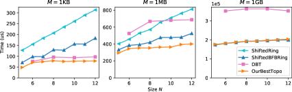
Figure 6: Comparing allreduce runtimes from experiments on testbed at $M\!=\!1\textnormal{KB}$, 1MB, and 1GB. The topologies we used for “OurBestTopo” are listed in Table 5.

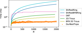
Figure 7: Comparing theoretical allreduce runtimes from analytical model at large $N$s for $d\!=\!4$, $\alpha\!=\!10\mu s$, and $M/B\!=\!1\textnormal{MB}/100\textnormal{Gbps}$.

8.1 Direct-Connect Optical Testbed

Our testbed consists of 12 servers, each with an NVIDIA A100 GPU [9] and a 100 Gbps HP NIC [10], configured as 4x25Gbps breakout interfaces [8]. The NICs are directly connected via a Telescent optical patch panel [11]. Our testbed can realize topologies by reconfiguring the patch panel. We limit our evaluation to bidirectional topologies. While unidirectional topologies can be realized by configuring the patch panel in simplex mode, the requisite overlay routing for the reverse path traffic (acks, etc.) is currently only supported using routing rules performed by the host kernel as opposed to the NIC, leading to unpredictable RTTs. Therefore, we can functionally validate unidirectional topologies on our testbed, but we cannot accurately evaluate their performance. Note that newer NICs [6, 1] do support hardware offloading for these rules, which we will examine in future work.

8.2 Experiment Setup

Baselines: We evaluate against the following baselines at $d\!=\!4$: (1) ShiftedRing, which improves upon NCCL ring [5], is the topology used by TopoOpt [71] for data-parallel training. The topology is a superposition of two bidirectional rings, each allreducing half of the data. (2) ShiftedBFBRing uses ShiftedRing topology and augments it with our BFB schedule on each ring (§E.1) to reduce node latency. (3) Double Binary Tree (DBT), also implemented in NCCL, uses the topology and schedule from [58, 35].

Methodology: We use the MSCCL runtime [19, 24, 49] to evaluate the topologies and schedules. We sweep through several key schedule parameters, such as the protocol (Simple or LL), number of channels (1, 2, 4, or 8), different degrees of pipelining for the DBT baseline, etc., and choose the best-performing schedule for each data size. For DNN training, we pass our schedules to PyTorch with the MSCCL backend.

8.3 AllReduce Experiments

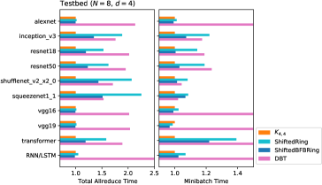
(a) Testbed training results (normalized by $K_{4,4}$)

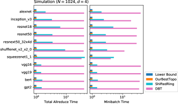
(b) Simulation results (normalized by lower bound)

Figure 8: Comparison with baseline topologies in DNN training. Figure (a) shows results from actual training on our testbed of 8 NVIDIA A100 GPUs. All models are using batch size 64. The total allreduce time is the sum of the allreduce time of all layers in the model. Figure (b) shows the simulation results with $N\!=\!1024$, $\alpha\!=\!10\mu$s, $B\!=\!100\text{Gbps}$, and $d\!=\!4$. For each model, the “OurBestTopo” is chosen from Table 4 by picking the topology with minimum allreduce time. The exact topology used for each model is in Appendix Table 8. The ready timestamps of layers were gathered from running models on NVIDIA A100 GPU.

Figure 6 shows experiment results for varying topology sizes $N$ and data sizes $M$. Table 5 shows our topologies at each $N$ generated by our topology finder (§5.4). We observe that in the small data regime ($M\!=\!1$KB), our solution beats shifted ring by a significant margin (at $N\!=\!12$, $\sim\!\!60\%$ and $\sim\!\!75\%$ lower than ShiftedBFBRing and ShiftedRing, respectively) and also outperforms DBT ($\sim\!\!20\%$ at $N\!=\!8,10,12$). At small data sizes, the runtime is dominated by node latency $T_{L}$, and hence, we can significantly outperform ShiftedRing, which has linear instead of logarithmic $T_{L}$ growth with respect to $N$.

In the large data regime ($M\!=\!1$GB), our solution beats DBT by a significant margin ($\sim\!\!50\%$ lower at $N\!=\!8,10,12$) and matches the performance of shifted ring. At large data sizes, the runtime is dominated by BW runtime $T_{B}$. Since the shifted ring is BW-optimal, we can only match its performance. Due to the influence of both node latency and BW runtime at intermediate data sizes ($M\!=\!1$MB), our solution outperforms both shifted rings (at $N\!=\!12$, $\sim\!\!50\%$ and $\sim\!\!25\%$ lower than ShiftedRing and ShiftedBFBRing, respectively) and DBT ($\sim\!\!45\%$ at $N\!=\!8,10,12$) in this regime. Note that although our gains over shifted ring diminish as $M$ grows, future increases in hardware bandwidth will enhance gains at large $M$ due to $T_{L}$ playing a more significant role.

Figure 7 shows the runtime comparison for large $N$ based on our analytical model. Topologies generated by our topology finder perform orders of magnitude faster than ShiftedRing and ShiftedBFBRing ($\sim\!\!100\times$ and $\sim\!\!50\times$, respectively, near $N\!=\!2000$) due to their linear growth in $T_{L}$ with respect to $N$. Although DBT’s node latency is logarithmic, its poor BW performance also leads to significantly higher total runtime ($\sim\!\!10\times$ near $N\!=\!2000$). We also add 2D torus for comparison due to its popularity in datacenters and supercomputers. We use traditional torus schedule [57] mentioned in §5.3 and BFB torus schedule. Our topologies also outperform both ($\sim\!\!5\times$ and $\sim\!\!2.5\times$, respectively, near $N\!=\!2000$) due to their square root node latency. For a detailed analysis of our topologies at large $N$s, §G shows analysis in different $\alpha,M/B$.

Note that on both ShiftedRing and 2D torus, BFB schedule outperforms traditional schedules by a large margin in testbed experiments and analytically at large $N$. This is due to BFB’s 2$\times$ improvement on $T_{L}$ over naive ring allreduce (§E.1).

In summary, the results show that (1) efficient scheduling (BFB), when applied to existing topologies (ShiftedRing, 2D torus), yields performance gains; (2) joint optimization of topology and schedule leads to further improvement; and (3) the best topology/schedule depends on hardware ($N,\alpha,B$) and workload ($M$) parameters, underscoring the need for parameter-aware topology-schedule search.

8.4 DNN Training Experiments

Figure 8(a) shows experiment results of total allreduce time and per-minibatch time across all layers on several common DNN models. Our solution $K_{4,4}$ improves total allreduce time by 30% and 50% (minibatch time by 10% and 25%) on average against ShiftedRing and DBT, respectively. ShiftedBFBRing outperforms ShiftedRing in every model due to its improvement in node latency. Since optimizations such as wait-free backpropagation [74] overlap computation and communication, some improvements in collective communication are hidden by the computation within the minibatch time.

The gains depend on layer sizes in each model. For models with many large layers (e.g., vgg16 [62]), BW-optimal topologies like $K_{4,4}$ and shifted rings are better. For models with mostly small layers (e.g., squeezenet1_1 [32]), topologies with low node latency like $K_{4,4}$, DBT, and ShiftedBFBRing perform better. Since our $K_{4,4}$ topology is both node latency and BW optimal, it has the best performance across almost all models. A few exceptions show shifted rings marginally beat $K_{4,4}$, which, we argue, are due to the ring’s simpler schedule implementation. The marginal gap could be eliminated with a more fine-tuned compiler and runtime, and even in such exceptions, our ShiftedBFBRing still outperforms ShiftedRing.

$N$	SCCL				TACCL w/o Symmetry				TACCL w/ Symmetry				BFB
	$c\!=\!1$	$c\!=\!2$	$c\!=\!3$	$c\!=\!4$	$c\!=\!1$	$c\!=\!2$	$c\!=\!3$	$c\!=\!4$	$c\!=\!1$	$c\!=\!2$	$c\!=\!3$	$c\!=\!4$
Hypercube
4	0.59	0.64	0.68	0.72	0.89	0.50	0.83	0.75	0.62	0.51	0.71	0.60	$<\!\!0.01$
8	0.86	1.22	1.86	2.48	96.9	807	63.2	1800	7.97	645	7.39	1801	$<\!\!0.01$
16	21.4	48.4	130	573	1801	1801	1801	1802	1801	n/a	n/a	n/a	$<\!\!0.01$
32	$>\!\!10^{4}$	$>\!\!10^{4}$	$>\!\!10^{4}$	$>\!\!10^{4}$	1802	n/a	n/a	n/a	n/a	n/a	n/a	n/a	0.03
64	$>\!\!10^{4}$	$>\!\!10^{4}$	$>\!\!10^{4}$	$>\!\!10^{4}$	n/a	n/a	n/a	n/a	n/a	n/a	n/a	n/a	0.17
1024	$>\!\!10^{4}$	$>\!\!10^{4}$	$>\!\!10^{4}$	$>\!\!10^{4}$	n/a	n/a	n/a	n/a	n/a	n/a	n/a	n/a	52.7
2D Torus ($n\times n$)
4	0.61	0.63	0.67	0.76	0.68	0.50	0.82	0.72	0.45	0.51	0.76	0.64	$<\!\!0.01$
9	1.00	1.51	2.22	3.44	1801	189	67.8	262	88.6	71.1	67.8	105	$<\!\!0.01$
16	17.5	60	131	603	1801	1801	1801	1802	1801	1801	1801	n/a	$<\!\!0.01$
25	3286	5641	$>\!\!10^{4}$	$>\!\!10^{4}$	1802	1802	1803	n/a	1802	n/a	n/a	n/a	0.01
36	$>\!\!10^{4}$	$>\!\!10^{4}$	$>\!\!10^{4}$	$>\!\!10^{4}$	n/a	n/a	n/a	n/a	n/a	n/a	n/a	n/a	0.03
2500	$>\!\!10^{4}$	$>\!\!10^{4}$	$>\!\!10^{4}$	$>\!\!10^{4}$	n/a	n/a	n/a	n/a	n/a	n/a	n/a	n/a	61.1

Table 6: Comparing allgather schedule generation runtimes (in seconds) of SCCL, TACCL, and BFB. The setup of SCCL is to generate schedules with least number of comm steps. Both SCCL and TACCL were run with chunks=1,2,3,4 (number of chunks per shard), and TACCL was run w/ and w/o manually set topology symmetry. “n/a” indicates where TACCL reports an error due to failure to generate a solution within its 1800s time limit for MILP solver.

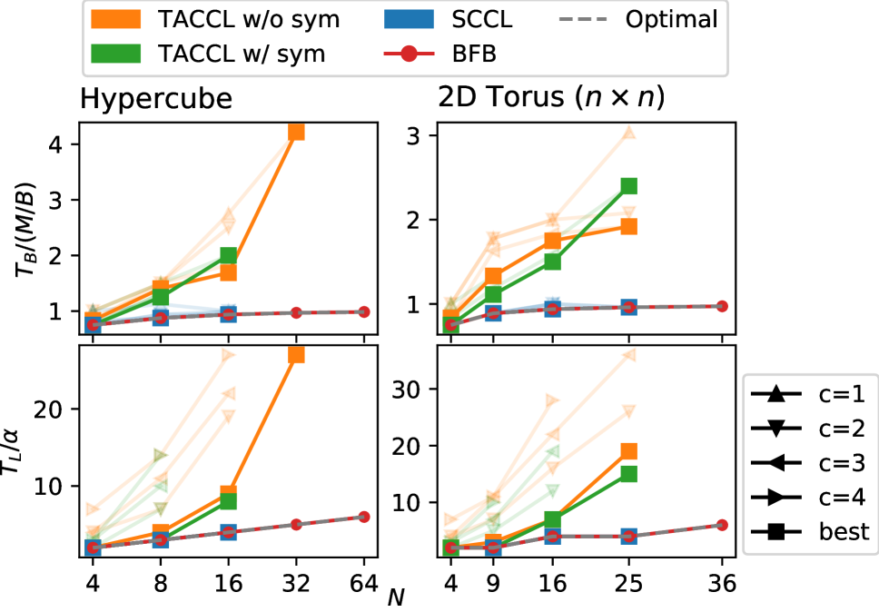
Figure 9: Comparing theoretical performances of schedules from Table 6. The figure shows both $T_{L}$ and $T_{B}$ of the schedules, along with the theoretical optimal. For SCCL and TACCL, the solid lines show the best results from parameter sweeps. The inferior ones are dimmed.

Large-Scale Simulation We simulate DNN training at a much larger scale ($N\!=\!1024$) than our testbed permits. We execute each model on a standalone NVIDIA A100 GPU and gather each layer’s ready timestamp. We then employ a simulation methodology based on [46] that uses the collected timestamps and the estimated allreduce time to simulate wait-free backpropagation [74]. The simulation overlaps real compute time and estimated allreduce time following two rules: (1) if there is no pending allreduce, we initiate an allreduce for the next ready layer as soon as it becomes ready; (2) if an allreduce is pending, all layers that become ready while waiting are buffered and then allreduced together immediately after the pending allreduce completes. The ready timestamps are unaffected by allreduce, so computation and communication are overlapped. We run simulations on various DNNs. For each model, we compute the best of our Pareto-efficient topologies (Table 4) and compare it against ShiftedRing and DBT. The results are in Figure 8(b). Across the eleven DNNs, our topologies have on average 6.7$\times$ and 38$\times$ lower allreduce time (2.6$\times$ and 28$\times$ lower minibatch training time) than ShiftedRing and DBT respectively, while being only 1.5% on average (at most 5.7%) above the theoretical lower bound of allreduce time and 0.7% on average (at most 1.7%) above the lower bound of minibatch time.

In summary, allreduce speedups translate to speedups in DNN training, increasing with scale.

8.5 BFB Schedule Generation Evaluation

We evaluate schedule generation from two aspects: schedule generation runtime and the performance of generated schedules. In §8.5.1, we compare BFB with state-of-the-art schedule generations: SCCL [19] and TACCL [60], in both generation runtime and theoretical schedule performance. In §8.5.2, we compare the performance of torus schedules generated by BFB, traditional torus scheduling [57], SCCL, and TACCL on supercomputing torus clusters with up to 54 nodes.

8.5.1 Schedule Generation

In schedule generation, SCCL and TACCL are the closest in spirit to BFB schedule generation. Table 6 shows the runtime comparison between SCCL, TACCL, and BFB when generating allgather schedules for hypercube and 2D torus. Both SCCL and TACCL use NP-hard optimization to generate schedules. SCCL, which uses an SMT solver, fails to generate a schedule within $10^{4}$ seconds beyond $N\!=\!30$. TACCL formulates the scheduling problem as a mixed integer linear program (MILP). It sets an 1800s time limit for its MILP solver, after which it will return the best solution found up to that point. However, for larger topologies, TACCL’s solver fails to find a solution within the time limit, resulting in an error. In comparison, BFB schedule generation is faster by orders of magnitude due to its polynomial-time generation.

In terms of theoretical schedule performance, Figure 9 compares the node latency and BW runtime of generated schedules. Given a topology, SCCL and TACCL need to perform a sweep across parameters such as the number of chunks and symmetry. They have to generate schedules for different parameter sets to identify the high-performance ones, unlike BFB, which has no parameter. In Figure 9, the schedules of SCCL and BFB can both achieve exact optimality, but TACCL’s have significantly worse performance, especially at large $N$s. SCCL is uniquely capable of generating all Pareto-efficient schedules. However, due to the prohibitive runtime of parameter sweep, SCCL can only do so for very small $N$s.

In summary, BFB schedule generation is highly scalable. It is orders of magnitude faster than state-of-the-art generations and requires no parameter sweep, while still producing schedules with top theoretical performance.

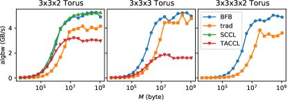
Figure 10: Comparing allreduce performances of torus schedules generated by BFB, traditional torus scheduling [57], SCCL, and TACCL on Frontera [64] supercomputer. The $y$-axis is algorithmic bandwidth (algbw), computed as $M$ divided by end-to-end runtime. SCCL fails to generate a schedule for $3\!\!\times\!\!3\!\!\times\!\!3$ and $3\!\!\times\!\!3\!\!\times\!\!3\!\!\times\!\!2$ tori, and TACCL fails to generate a schedule for $3\!\!\times\!\!3\!\!\times\!\!3\!\!\times\!\!2$ torus within the time limits.

8.5.2 Supercomputing Allreduce Experiments

In the supercomputing setting, we run torus schedules generated by BFB, traditional torus scheduling [57], SCCL, and TACCL on Frontera [64] supercomputer at the Texas Advanced Computing Center (TACC) [7]. The cluster consists of 396 nodes in a 6D torus direct-connect topology. Each node is equipped with an Intel Xeon Platinum 8280 CPU and a Rockport NC1225 network card, capable of delivering 25 Gbps per link, with degree 12. At higher degree, however, the total BW of a single node is bottlenecked by the 100 Gbps host BW of PCIe Gen3 x16. Finally, the schedules are lowered and run using Intel oneCCL [3] + libfabric [4].

We run schedules on two types of sub-torus within the cluster: equal-dimension ($3\!\!\times\!\!3\!\!\times\!\!3$) and unequal-dimension ($3\!\!\times\!\!3\!\!\times\!\!2$ & $3\!\!\times\!\!3\!\!\times\!\!3\!\!\times\!\!2$). As shown in Figure 10, BFB schedules achieve the highest performance in all settings. As mentioned in §6.2, the traditional torus schedule can only achieve high BW performance in tori with equal dimensions. At large $M$, it matches BFB’s performance in $3\!\!\times\!\!3\!\!\times\!\!3$ torus but significantly underperforms in $3\!\!\times\!\!3\!\!\times\!\!2$ and $3\!\!\times\!\!3\!\!\times\!\!3\!\!\times\!\!2$, where BFB has 29% and 42% higher algbw on average for $M\!\geq\!100$MB. At small to intermediate $M$ ($<\!100$MB), BFB outperforms traditional schedules by 3.1$\times$ on average in all settings due to its 2$\times$ improvement in node latency and higher BW performance.

As for SCCL and TACCL, we adhere to the same time limits and parameter sweeps as in §8.5.1 and select the best result at each $M$ from all parameter sets. In $3\!\!\times\!\!3\!\!\times\!\!2$ torus, SCCL is able to generate an optimal schedule, matching BFB’s performance across all $M$. However, it fails to generate a schedule within $10^{4}$ seconds for other larger tori. TACCL can only generate schedules in $3\!\!\times\!\!3\!\!\times\!\!2$ and $3\!\!\times\!\!3\!\!\times\!\!3$, and its schedules underperform BFB’s by a large margin. One additional observation is that the algbw of BFB at large $M$ hardly changes from 18-node ($3\!\!\times\!\!3\!\!\times\!\!2$) to 54-node ($3\!\!\times\!\!3\!\!\times\!\!3\!\!\times\!\!2$) torus. This can be explained by the fact that BFB schedules have mathematically achieved allreduce BW optimality ($\frac{2M}{B}\!\cdot\!\frac{N-1}{N}$), which remains nearly constant as $N$ increases.

In summary, BFB schedule generation produces top-performing schedules for supercomputing torus clusters, even in unequal-dimension tori, unlike traditional torus scheduling. State-of-the-art schedule generations are limited by scalability, even if not schedule performance.

9 Concluding Remarks

Collective communications are critical to both large-scale ML training and HPC workloads. Current network architectures do not exploit the regular patterns of distributed data flow embedded in these collectives and often suffer from high node latency or bandwidth contention. In this paper, we demonstrated a general, highly scalable, and automated algorithmic framework for optimizing topology and schedule generation for collective communications by leveraging scalable graph-theoretic approaches. Our evaluation demonstrates significant performance benefits using multiple testbeds and large-scale simulations for both collectives and training jobs.

10 Acknowledgements

This research was developed with funding from the Defense Advanced Research Projects Agency (DARPA) under Contract No.HR001120C0089. The views, opinions and/or findings expressed are those of the author and should not be interpreted as representing the official views or policies of the Department of Defense or the U.S. Government.

Appendix

In this appendix, we give formal mathematical definitions and analysis of various techniques and concepts mentioned in the main text. To summarize,

• §A gives formal definitions of reduce-scatter/allgather schedule and how one can be transformed into another.

• §B gives formal definitions of node latency and bandwidth optimality, along with discussions on optimal allreduce schedule and computational cost of reduction.

• §C provides formal definitions of expansion techniques and optimality analysis of their expanded schedules.

• §D provides optimality analysis of BFB schedule generation and discusses variant formulations that support generating schedules for a fixed number of chunks and for heterogeneous network topology.

• §E discusses various generative topologies and the performance of their generated BFB schedules.

• §F shows how to convert unidirectional topologies/schedules into bidirectional ones.

• §G gives an analysis of Pareto-efficient topologies/schedules under different hardware and workload specifications.

• §H shows experiment results on $\alpha$-$\beta$ cost model validation.

• §I presents experiment results that compare BFB schedule generation with communication solutions on switch networks: NCCL [5] and recursive halving & doubling.

• §J provides proofs of all theorems in this paper.

• §K contains supplementary tables and figures. In particular, Table 9 gives a summary of topologies in this paper.

Appendix A Reduce-Scatter & Allgather

We use tuple $((v,C),(u,w),t)$ to denote that $u$ sends $v$’s chunk $C$ to $w$ at comm step $t$. Node $v$ is the source and destination node of chunk $C$ in allgather and reduce-scatter respectively. A communication schedule is thus a collection of tuples.

Definition 6 (Allgather).

An algorithm $(G,A)$ is an allgather algorithm if for arbitrary $x\in S$ and distinct $u,v\in V_{G}$, there exists a sequence in $A$:

$$((v,C_{1}),(w_{0},w_{1}),t_{1}),((v,C_{2}),(w_{1},w_{2}),t_{2}),\dots{\\ }((v,C_{n}),(w_{n-1},w_{n}),t_{n}),$$

where $w_{0}\!=\!v$, $w_{n}\!=\!u$, $t_{1}\!<\!t_{2}\!<\!\dots\!<\!t_{n}$, and $x\!\in\!C_{1}\!\cap C_{2}\!\cap\dots\cap C_{n}$.

This sequence serves to broadcast $x$ from $v$ to $u$. A reduce-scatter algorithm has the same definition except $w_{0}\!=\!u$, $w_{n}\!=\!v$. In reduce-scatter, we assume any chunk received by a node is immediately reduced with the node’s local chunk.

In this paper, many of the techniques are discussed under allgather only. We will show that anything holds in either reduce-scatter or allgather has an equivalent version for the other collective operation. To do so, we use the concept of transpose graph from graph theory and define reverse schedule. We say a schedule $A$ is for topology $G$ if every $((v,C),(u,w),t)\in A$ satisfies $u,v,w\in V_{G}$ and $(u,w)\in E_{G}$.

Definition 7 (Reverse Schedule).

Suppose $A$ is a schedule for $G$. A reverse schedule $A^{T}$ of $A$ is a schedule for transpose graph $G^{T}$ such that $((v,C),(u,w),t_{\max}-t+1)\in A^{T}$ iff $((v,C),(w,u),t)\in A$, where $t_{\max}$ is the max comm step in $A$.

It is trivial to see that $T_{L}(A)=T_{L}(A^{T})$ and $T_{B}(A)=T_{B}(A^{T})$. Note that $(u,w)\in E_{G^{T}}$ if and only if $(w,u)\in E_{G}$ by definition of transpose graph.

Theorem 3.

If $A$ is a reduce-scatter/allgather schedule for $G$, then $A^{T}$ is an allgather/reduce-scatter schedule for $G^{T}$.

Theorem 3 has the following two corollaries:

Corollary 3.1.

Suppose $G\mapsto f(G)$ is a function to construct reduce-scatter/allgather schedule given graph $G$, then $G\mapsto f(G^{T})^{T}$ is a function to construct allgather/reduce-scatter schedule given graph $G$.

Corollary 3.2.

Suppose $(G,A)\mapsto(f(G),f(A))$ is a mapping within reduce-scatter/allgather algorithms, then $(G,A)\mapsto(f(G^{T})^{T},f(A^{T})^{T})$ is a mapping within allgather/reduce-scatter algorithms.

For example, the line graph expansion in §5.1 can be seen as a mapping within allgather, and the BFB linear program (3) can be seen as a function to construct allgather schedule. Thus, Corollary 3.1 and 3.2 have shown that they both have equivalent versions in reduce-scatter.

In undirected topology, it is well-known that reduce-scatter and allgather are a pair of dual operations such that one can be transformed into another by reversing the communication in schedule [21]. It is similar for directed topology but with extra requirement and more complicated transformation. We define the following property for directed graphs:

Definition 8 (Reverse-Symmetry).

A digraph $G$ is reverse-symmetric if it is isomorphic to its own transpose graph $G^{T}$.

In graph theory, there is a similar concept called skew-symmetric graph. Reverse-symmetry is a weaker condition than skew-symmetry.

We define a way to transform the schedule for $G$ into a schedule for $G^{T}$ based on graph isomorphism:

Definition 9 (Schedule Isomorphism).

Suppose $G$ and $G^{\prime}$ are isomorphic. Let $f:V_{G}\to V_{G^{\prime}}$ be the graph isomorphism and $A$ be a schedule for $G$, then $f(A)$ is a schedule for $G^{\prime}$ that $((f(v),C),(f(u),f(w)),t)\!\in\!f(A)$ iff $((v,C),(u,w),t)\!\in\!A$.

Theorem 4.

Suppose $G$ is reverse-symmetric. Let $G^{T}$ be the transpose graph, and let $f:V_{G^{T}}\to V_{G}$ be the isomorphism from $G^{T}$ to $G$. If $(G,A)$ is a reduce-scatter/allgather algorithm, then $(G,f(A^{T}))$ is an allgather/reduce-scatter algorithm with $T_{L}(f(A^{T}))=T_{L}(A)$ and $T_{B}(f(A^{T}))=T_{B}(A)$.

Theorem 4 establishes that given any reverse-symmetric topology, if we have either reduce-scatter or allgather, then we can construct both reduce-scatter and allgather. Since allreduce can be achieved by applying a reduce-scatter followed by an allgather, we only need one of reduce-scatter and allgather to construct a complete allreduce algorithm. Furthermore, if the reduce-scatter or allgather algorithm has runtime $T$, then the resulting allreduce algorithm has runtime $2T$.

Most of our base topologies are reverse-symmetric (Table 9). In addition, all of our expansion techniques also preserve reverse-symmetry. Thus, one can almost always use Theorem 4 to derive reduce-scatter and allreduce schedules from allgather schedule on our synthesized topologies. For non-reverse-symmetric topologies like generalized Kautz graph, one can apply Corollary 3.1 or 3.2 to construct reduce-scatter and allgather separately.

Appendix B Topology-Schedule Optimality

Because our cost model is only concerned with node latency and BW runtime, the optimality of reduce-scatter/allgather algorithm is only related to node latency optimality and BW optimality in this paper. Note that we also consider topology as a dimension that can be optimized, so optimality is discussed in the space of all topology-schedule combinations, i.e., algorithms by our definition.

B.1 Node Latency Optimality

Definition 10 (Node Latency Optimal).

Given an $N$-node degree-$d$ reduce-scatter/allgather algorithm $(G,A)$, if any other $N$-node degree-$d$ reduce-scatter/allgather algorithm $(G^{\prime},A^{\prime})$ satisfies $T_{L}(A^{\prime})\!\geq\!T_{L}(A)$, then $(G,A)$ is node latency optimal.

Because in reduce-scatter/allgather, every node needs to send a shard of data to every other node, the number of comm steps is lower bounded by the graph diameter:

Theorem 5.

Every reduce-scatter/allgather algorithm $(G,A)$ satisfies $T_{L}(A)\!\geq\!\alpha\cdot D(G)$, where $D(G)$ is the diameter of $G$.

Because we can always construct a BFB schedule $A$ for topology $G$ with $T_{L}(A)=\alpha\cdot D(G)$, it follows the corollary:

Corollary 5.1.

An $N$-node degree-$d$ reduce-scatter/allgather algorithm $(G,A)$ is node latency optimal if and only if

$$T_{L}(A)=\alpha\cdot D(G)=\alpha\cdot\min\{D(G^{\prime}):|V_{G^{\prime}}|=N,\deg(G^{\prime})=d\}.$$

The minimum diameter of a directed graph given a number of vertices and degree is still an open question. One can check degree/diameter problem [50] for more information. However, as a close upper bound of number of vertices given degree and diameter, the Moore bound for digraph is sufficient to tell the node latency optimality in most cases.

Definition 11 (Moore Bound).

Let $G$ be any degree-$d$ digraph of diameter $k$. The Moore bound is an upper bound on the number of vertices in $G$:

$$M_{d,k}=\sum_{i=0}^{k}d^{i}=\frac{d^{k+1}-1}{d-1}.$$

Definition 12 (Moore Optimal).

Let $(G,A)$ be an $N$-node degree-$d$ reduce-scatter/allgather algorithm with $T_{L}(A)=k\alpha$, then $(G,A)$ is Moore optimal if $N>M_{d,k-1}$.

Because for any degree-$d$ digraph $G$, $D(G)\geq k$ must be true as long as $|V_{G}|>M_{d,k-1}$, Moore optimality is a stronger condition than node latency optimality. We define a function $T^{*}_{L}$ such that $T^{*}_{L}(N,d)$ is equal to the Moore optimal node latency of $N$-node degree-$d$ reduce-scatter/allgather algorithms.

B.2 Bandwidth Optimality

Definition 13 (Bandwidth Optimal).

Given an $N$-node degree-$d$ reduce-scatter/allgather algorithm $(G,A)$, if any other $N$-node degree-$d$ reduce-scatter/allgather algorithm $(G^{\prime},A^{\prime})$ satisfies $T_{B}(A^{\prime})\geq T_{B}(A)$, then $(G,A)$ is BW-optimal.

In reduce-scatter/allgather, each node needs to send/receive at least $M\cdot\frac{N-1}{N}$ amount of data. Thus, the following holds:

Theorem 6.

$\frac{M}{B}\cdot\frac{N-1}{N}$ is a lower bound of $T_{B}(A)$ for any $N$-node reduce-scatter/allgather algorithm $(G,A)$.

Note that one can always construct a ring of degree $d$ by sending $d$ parallel edges from one node to the next node. The trivial ring reduce-scatter/allgather schedule has $\frac{M}{B}\cdot\frac{N-1}{N}$ BW runtime. Therefore, we have:

Corollary 6.1.

An $N$-node reduce-scatter/allgather algorithm $(G,A)$ is BW-optimal if and only if $T_{B}(A)=\frac{M}{B}\cdot\frac{N-1}{N}$.

We define a function $T^{*}_{B}$ such that $T^{*}_{B}(N)=\frac{M}{B}\cdot\frac{N-1}{N}$ is the optimal BW runtime of $N$-node reduce-scatter/allgather algorithms. From Corollary 6.1, we have the following necessary and sufficient condition for BW optimality:

Theorem 7.

An allgather algorithm $(G,A)$ is BW-optimal if and only if:

1. $\frac{1}{B/d}\!\sum_{((v,C),(u,w))\in A_{t}}\!|C|\!=\!T_{B}(A_{t})$ for all $(u,v)\!\in\!E_{G}$ and $t\!\in\!\{1,\dots,t_{\max}\}$. $A_{t}$ is the subschedule of $A$ at comm step $t$.

2. Pick any distinct $u,v\in V_{G}$. For each $x\in S$, there exists a unique $((v,C),(w,u),t)\in A$ such that $x\in C$.

Condition 1 ensures that at each comm step, every link of topology $G$ has equal workload, so no link finishes early and results in waste of bandwidth. Condition 2 ensures that no piece of data is received twice by some node, so no duplicated send exists.

B.3 Allreduce Optimality

In this paper, we construct an allreduce algorithm through a reduce-scatter followed by allgather. In such construction, the lower bound of allreduce algorithm is $2(T^{*}_{L}(N,d)+T^{*}_{B}(N))$. To compare this with the lower bound of any allreduce construction, in [54], the authors have proved that $2T^{*}_{B}(N)$ is indeed the lower bound of BW runtime of any allreduce algorithm. As for node latency, a reduce-scatter followed by allgather has at least $2D(G)$ number of comm steps, so $2T^{*}_{L}(N,d)$ is the lower bound of node latency. Although one can use all-to-all to construct an allreduce with number of comm steps equal to one diameter $D(G)$ (lower bound being $T^{*}_{L}(N,d)$ instead of $2T^{*}_{L}(N,d)$), the lower bound of BW runtime for all-to-all is $\frac{M}{B}\cdot(N-1)=N\cdot T^{*}_{B}(N)$, which is much worse than $2T^{*}_{B}(N)$.

There is also another way of constructing allreduce: reduce followed by broadcast. In such an approach, the number of comm steps can be twice the radius of $G$ instead of twice the diameter. However, the Moore bound for graph diameter also applies to graph radius, so $2T^{*}_{L}(N,d)$ is still a lower bound of allreduce via reduce+broadcast. By Theorem 16, the node latency optimal allreduce via reduce+broadcast is at most $2\alpha$ lower than the node latency of generalized Kautz graph can do with reduce-scatter plus allgather. Furthermore, reduce+broadcast is usually poor in BW performance.

B.4 Computational Cost

In this paper, we omit the computational cost of reduction operation in performance analysis. While this approach is commonly adopted in previous literature [70, 19, 60, 58], we give a formal reasoning why this approach is legitimate. It is not only because computational cost is generally orders of magnitude lower than network cost, but also because computational cost can be incorporated into network cost.

Assume a cost model where computation and network communication do not overlap at each node. In particular, at each comm step of reduce-scatter, the computation to reduce chunks happens immediately after the node receives all chunks and before the node starts to send out chunks for the next comm step. We adopt notations from [21], where $\gamma$ denotes the computational time cost per size of data. Like node latency and BW runtime, we also let $T_{C}(A)$ be the total time spent on computation by schedule $A$. As argued in [21], a lower bound of computational cost is $T_{C}\geq M\cdot\gamma\cdot\frac{N-1}{N}$ for both reduce-scatter and allreduce, which is identical to the BW optimality of reduce-scatter and half of that of allreduce. The following theorem shows that BW runtime of a schedule can act as an upper bound for the computational time.

Theorem 8.

Given a reduce-scatter algorithm $(G,A)$, suppose $T_{B}(A)=\frac{M}{B}\cdot y$, then $T_{C}(A)\leq M\cdot\gamma\cdot y$.

The rationale behind Theorem 8 is that the amount of computation for any node at a given comm step equals the amount of data the node receives during that comm step. Thus, as we balance network transmission, it naturally leads to a more balanced computation. With Theorem 8, if the BW runtime of some allreduce schedule $A$ is $T_{B}(A)=2\frac{M}{B}\cdot y$, then $T_{B}(A)+T_{C}(A)\leq M\cdot(\frac{2}{B}+\gamma)\cdot y$. We can thus simply define $B^{\prime}=(\frac{1}{B}+\frac{\gamma}{2})^{-1}$, and then $2\frac{M}{B^{\prime}}\cdot y$ can represent the sum of BW runtime and computational runtime altogether. The value of $y$ is all that matters. The following corollary shows that if an algorithm is BW-optimal, then such representation is exact.

Corollary 8.1.

If allreduce algorithm $(G,A)$ is BW-optimal, i.e., $T_{B}(A)\!=\!2\frac{M}{B}\!\cdot\!\frac{N-1}{N}$, then $T_{C}(A)\!=\!M\!\cdot\!\gamma\!\cdot\!\frac{N-1}{N}$ and $T_{B}(A)+T_{C}(A)\!=\!2M\!\cdot\!(\frac{1}{B}+\frac{\gamma}{2})\!\cdot\!\frac{N-1}{N}$.

When profiling a testbed, one can simply derive the value of $\frac{1}{B}+\frac{\gamma}{2}$ using BW-optimal topologies and use it as the new $1/B$ to apply the results of this paper. While it is still possible for two schedules with the same BW runtime to have different computational runtimes, such difference is bounded by the aforementioned theorems and orders of magnitude smaller than BW runtime.

Appendix C Optimality of Expansion Techniques

In this section, we provide formal definitions and detailed performance analysis of expansion techniques.

C.1 Line Graph Expansion

See 1 See 2

The following theorem gives the performance of the expanded schedule: See 1 From Theorem 1, one can see that the performance of the expanded schedule depends on that of the base schedule. Theorem 1 makes an implicit assumption that $T_{B}(A_{G},M,B)\!=\!\tau(M/B)$ for some constant $\tau$. This assumption, suggesting that $T_{B}$ scales linearly with data size and inversely with bandwidth, should hold for any reasonably designed schedule.

Consequently, if we apply line graph expansion $n$ times, the performance of the expanded schedule is:

Corollary 1.2.

Given a $d$-regular topology $G$, if $(G,A_{G})$ is an $N$-node allgather algorithm with $T_{B}(A_{G},M,B)\!=\!\tau(M/B)$ for some constant $\tau$, then $(L^{n}(G),A_{L^{n}(G)})$ is a $d^{n}N$-node allgather algorithm satisfying:

$$T_{L}(A_{L^{n}(G)})=T_{L}(A_{G})+n\alpha,$$ (5)

$$T_{B}(A_{L^{n}(G)})\leq T_{B}(A_{G})+\frac{M}{B}\cdot\frac{d}{d-1}\left(\frac{1}{N}-\frac{1}{d^{n}N}\right).$$ (6)

Speaking of optimality:

Theorem 9.

$(L^{n}(G),A_{L^{n}(G)})$ is Moore optimal if and only if $(G,A_{G})$ is Moore optimal.

See 2

As mentioned in the main text, by Theorem 2, the key metric for the quality of base graph is how large it is while achieving both Moore and BW optimality. Currently, our largest such base graph that works for any even degree is Hamming graph $H(2,\!1\!+\!d/2)$, which has $(1\!+\!d/2)^{2}\!=\!\Theta(d^{2})$ number of nodes. The corresponding line graph expanded topology is always Moore optimal and at most $O(1/d^{3})$ away from BW optimality by Theorem 2.

Line graph expansion is closely related to BFB schedule for two reasons: (1) most of our base topologies like complete bipartite graph and Hamming graph use BFB schedule as the base schedule, and (2) the line graph expansion of BFB schedule is still a BFB schedule. To see the performance bound in Theorem 1 is tight, we have the following results in the context of BFB schedule:

Theorem 10.

Let $A_{G}$ be a BFB allgather schedule for $G$ with $|N^{+}(u)|\!>\!1$ for all $u\in V_{G}$, then the expanded schedule $A_{L(G)}$ is a BFB allgather schedule for $L(G)$. In particular, if $A_{G}$ is the optimal BFB schedule for $G$, then $A_{L(G)}$ is the optimal BFB schedule for $L(G)$ satisfying:

$$T_{B}(A_{L(G)})=T_{B}(A_{G})+\frac{M}{B}\cdot\frac{1}{N}.$$ (7)

Corollary 10.1.

Let $A_{G}$ be a BFB allgather schedule for $G$ with $|N^{+}(u)|\!>\!1$ for all $u\in V_{G}$, then the expanded schedule $A_{L^{n}(G)}$ is a BFB allgather schedule for $L^{n}(G)$. In particular, if $A_{G}$ is the optimal BFB schedule for $G$, then $A_{L^{n}(G)}$ is the optimal BFB schedule for $L^{n}(G)$ satisfying:

$$T_{B}(A_{L^{n}(G)})=T_{B}(A_{G})+\frac{M}{B}\cdot\frac{d}{d-1}\left(\frac{1}{N}-\frac{1}{d^{n}N}\right).$$

C.2 Degree Expansion

See 3 See 4

Theorem 11.

Given a $d$-regular topology $G$ without self loops, if $(G,A_{G})$ is an $N$-node allgather algorithm with $T_{B}(A_{G},M,B)=\tau(M/B)$ for some constant $\tau$, then $(G*n,A_{G*n})$ is an $nN$-node allgather algorithm satisfying:

$$T_{L}(A_{G*n})=T_{L}(A_{G})+\alpha,$$ (8)

$$T_{B}(A_{G*n})=T_{B}(A_{G})+\frac{M}{B}\cdot\frac{n-1}{nN}.$$ (9)

Corollary 11.1.

If $(G,A_{G})$ is BW-optimal and $T_{B}(A_{G},M,B)\!=\!\tau(M/B)$ for some $\tau$, then $(G*n,A_{G*n})$ is BW-optimal.

Degree expansion preserves BW optimality. As for node latency of degree expanded topology, observe that $T_{L}^{*}(N,d)=\Theta(\log_{d}N)$ and $\log_{nd}nN<\log_{d}N$, so $T_{L}^{*}$ decreases as we apply degree expansion. Since $T_{L}$ increases in degree expansion, the node latency optimality is not preserved.

C.3 Cartesian Product Expansion

See 5 Definition 5 generalizes to Cartesian product of multiple digraphs: $G_{1}\square G_{2}\square G_{3}\!=\!(G_{1}\square G_{2})\square G_{3}$. The Cartesian product of $n$ identical digraphs is denoted as Cartesian power $G^{\square n}$.

Definition 14 (Schedule of Cartesian Power).

Given an allgather schedule $A_{G}$ for topology $G$ and $n\in\mathbb{N}$, construct the schedule $A_{G^{\square n}}$ for $G^{\square n}$:

1. Construct the schedule $A^{(1)}$ as follows:

2. For $j=1,\dots,n$, for each $((w,C),(u,v),t)\in A_{G}$, add

   $$(((\mathbf{x},w,\mathbf{z}),C),((\mathbf{y},u,\mathbf{z}),(\mathbf{y},v,\mathbf{z})),t+(j-1)t_{\max})$$

   to $A^{(1)}$ for all $\mathbf{x},\mathbf{y}\in V_{G}^{j-1}$ and $\mathbf{z}\in V_{G}^{n-j}$. $t_{\max}$ is the max comm step in $A_{G}$.

3. Similarly, construct $A^{(i)}$ for $i\!=\!2,\dots,n$ that each vertex $\mathbf{v}$ in $A^{(1)}$ is shifted by $i\!-\!1$ to $(\mathbf{v}[n\!-\!i\!+\!2\!:\!n],\mathbf{v}[1\!:\!n\!-\!i\!+\!1])$.

4. Divide each shard into $n$ equal-sized subshards. Construct schedule $A_{G^{\square n}}$ such that $A^{(i)}$ performs allgather over the $i$-th subshards of all nodes.

Theorem 12.

Given a $d$-regular topology $G$, if $(G,A_{G})$ is an $N$-node allgather algorithm with $T_{B}(A_{G},M,B)=\tau(M/B)$ for some constant $\tau$, then $G^{\square n}$ is an $nd$-regular topology, and $(G^{\square n},A_{G^{\square n}})$ is an $N^{n}$-node allgather algorithm satisfying:

$$T_{L}(A_{G^{\square n}})=n\cdot T_{L}(A_{G}),$$ (10)

$$T_{B}(A_{G^{\square n}})=T_{B}(A_{G})\cdot\frac{N}{N-1}\cdot\frac{N^{n}-1}{N^{n}}.$$ (11)

We then have the following corollary:

Corollary 12.1.

If $(G,A_{G})$ is BW-optimal and $T_{B}(A_{G},M,B)\!=\!\tau(M/B)$ for some $\tau$, then $(G^{\square n},A_{G^{\square n}})$ is BW-optimal.

Like degree expansion, Cartesian power expansion does not preserve node latency optimality.

We use BFB schedule generation when dealing with Cartesian product of distinct topologies:

Theorem 13.

Let $G_{1},G_{2},\dots,G_{n}$ be topologies that

1. $G_{1},\dots,G_{n}$ are nontrivial simple digraphs;

2. Every $G_{i}$ has BW-optimal BFB allgather schedule.

Then, the optimal BFB allgather schedule, i.e. the schedule generated by BFB LP (3), for $G_{1}\square\dots\square G_{n}$ is also BW-optimal. The node latency of the schedule equals $\alpha\cdot D(G_{1}\square\dots\square G_{n})\!=\!\alpha\cdot\sum_{i}D(G_{i})$.

The BFB schedule generation can also be used when individual topologies do not have BW-optimal BFB schedules; however, in such a case, we do not have performance bound for the schedule of the Cartesian product.

Appendix D BFB Schedule Generation

The LP formulation corresponding to $u_{2}$ in Figure 5 is:

$$\begin{array}[]{lr@{}ll}\text{minimize}&U_{u_{2},t}\phantom{x_{v_{1},w_{1}}}&&\\ \text{subject to}&\displaystyle x_{v_{1},(w_{1},u_{2}),t}&\leq U_{u_{2},t},&\\ &\displaystyle x_{v_{1},(w_{2},u_{2}),t}+x_{v_{2},(w_{2},u_{2}),t}&\leq U_{u_{2},t},&\\ &\displaystyle x_{v_{2},(w_{3},u_{2}),t}&\leq U_{u_{2},t},&\\ &\displaystyle x_{v_{1},(w_{1},u_{2}),t}+x_{v_{1},(w_{2},u_{2}),t}&=1,&\\ &\displaystyle x_{v_{2},(w_{2},u_{2}),t}+x_{v_{2},(w_{3},u_{2}),t}&=1,&\\ &0\leq x_{v,(w,u_{2}),t}&\leq 1.&\forall v,w\end{array}$$

Definition 15 (BFB schedule).

An allgather schedule $A$ for $G$ is a BFB schedule if $A$ satisfies: $((v,C),(w,u),t)\in A$ only if $d(v,u)=d(v,w)+1=t$.

Theorem 14.

A schedule $A$ for $G$ is a BFB allgather schedule if and only if the following are satisfied:

1. If $((v,C),(w,u),t)\in A$, then $d(v,u)=d(v,w)+1=t$;

2. For any distinct $u,v\in V_{G}$, the collection of chunks $\mathcal{C}_{v}=\{C\ |\ ((v,C),(w,u),t)\in A\}$ satisfies $S=\bigcup_{C\in\mathcal{C}_{v}}C$.

Condition 1 ensures the schedule follows the breadth-first broadcast order. Condition 2 ensures every node receives the entire shard from every other node and thus a valid allgather.

D.1 Optimality

Theorem 15.

If $A$ is a BFB schedule for $G$, then $T_{L}(A)=\alpha\cdot D(G)$.

There may exist many BFB schedules for a given topology $G$. They all have the same $T_{L}$ but may have different $T_{B}$s. Thus, the optimal BFB schedule is the one with the lowest $T_{B}$. Since every BFB schedule can be expressed as a solution to linear program (3), we have the following result:

Theorem 16.

Given any topology $G$, linear program (3) gives the optimal BFB schedule of $G$.

An important implication of Theorem 16 is that if we can show a BW-optimal BFB schedule exists for a topology $G$, then linear program $(\ref{lpmodel})$ is guaranteed to generate one. This has become an important tool for us to prove that BFB schedule generation can always generate BW-optimal schedules for some families of topologies. For the rest of this section, we show conditions that, if met by a topology, ensure it has a BW-optimal BFB schedule.

The following theorem shows the necessary and sufficient conditions for a BFB allgather schedule to be BW-optimal:

Theorem 17.

Suppose $(G,A)$ is a BFB allgather schedule. $(G,A)$ is BW-optimal if and only if:

1. There exists a sequence $N^{-}_{1},N^{-}_{2},\dots,N^{-}_{D(G)}\in\mathbb{N}$ such that for any $x\in\mathbb{N}$ and $u\in V_{G}$, $|N^{-}_{t}(u)|=N^{-}_{x}$.

2. For any $(w,u)\in E_{G}$, $\sum_{((v,C),(w,u))\in A_{t}}|C|=\frac{M}{N}|N^{-}_{t}(u)|/d=\frac{M}{N}N^{-}_{t}/d$.

We assume $G$ is $d$-regular. Condition 1 and 2 together ensure that at each comm step, all links have perfectly balanced workloads. In Theorem 13, we have already proven that a Cartesian product graph has BW-optimal BFB schedule if it is the product of graphs that each have a BW-optimal BFB schedule. Here, Theorem 17 also leads to the following sufficient condition for a bidirectional topology to have a BW-optimal BFB schedule:

Theorem 18.

There exists a BW-optimal BFB schedule for undirected graph $G$ if for every distance $x$, two of the following constants exist:

1. $N_{x}=|N_{x}(u)|$ for any $u\in V_{G}$;

2. $a_{x}=|N_{x}(u)\cap N_{x-1}(w)|$ for any $u\in V_{G}$ and $w\in N(u)$;

3. $b_{x}=|N(u)\cap N_{x-1}(v)|$ for any $u\in V_{G}$ and $v\in N_{x}(u)$.

Moreover, if two of $N_{x},a_{x},b_{x}$ exist, then the third one must also exist with $N_{x}=da_{x}/b_{x}$.

Note that in undirected graphs, we have $N^{+}_{x}(u)=N^{-}_{x}(u)=N_{x}(u)$. To understand these constants, $N_{x}$ is the number of data shards $u$ needs to receive at comm step $x$; $a_{x}$ is the number of data shards that can be transmitted by each link $(w,u)$ at comm step $x$; $b_{x}$ is the number of link $(w,u)$s that each data shard can use to transmit the data to $u$ at comm step $x$. These three constants collectively ensure that links are perfectly balanced with each link transmitting $\frac{M}{N}N_{x}/d=\frac{M}{N}a_{x}/b_{x}$ amount of data at comm step $x$.

Now, we give a necessary and sufficient condition for any topology to have a BW-optimal BFB schedule. The condition is derived based on the observation that the BFB optimization problem is equivalent to a job scheduling problem. In each comm step $t$, for each node $u$, we have a set of jobs $\{j_{1},j_{2},\dots,j_{m}\}$ (data from the source nodes $v\!\in\!N^{-}_{t}(u)$) and a set of processors $\{p_{1},p_{2},\dots,p_{d}\}$ (links from in-neighbors $w\!\in\!N^{-}(u)$). There exists a map $f$ from any job to a set of processors that $j_{i}$ can only be scheduled to the processors in $f(j_{i})$ (in-neighbor $w$s satisfying $d(v,u)=d(v,w)+1=t$). Assuming jobs can be arbitrarily divided into subjobs for parallel execution on multiple processors, the problem is how to schedule these jobs to processors so that workloads are balanced across all processors. We have the following result:

Theorem 19.

The workloads can be balanced if and only if there exists no subset $J\subseteq\{j_{1},j_{2},\dots,j_{m}\}$ such that

$$\frac{|J|}{\left|\bigcup_{j\in J}f(j)\right|}>\frac{m}{d}.$$

Note that there is an independent scheduling problem for each comm step $t$ and node $u$. Therefore, topology $G$ has a BW-optimal BFB schedule if and only if:

1. At each comm step $t$, $|N^{-}_{t}(u)|$ is the same for all $u\in V_{G}$.

2. The scheduling problem w.r.t. each $t$ and $u$ satisfies the condition in Theorem 19.

D.2 Discrete Chunked BFB Schedule

The BFB LP (3) makes an assumption that shards can be divided arbitrarily and infinitesimally. However, to compile the schedule into an executable form, one often needs a discrete chunked schedule, where each shard is divided into a fixed number of equal-sized chunks. In practice, $x_{v,(w,u),t}$s are usually solved to be rational numbers. We can divide each shard into a number of chunks equal to the LCM of $x_{v,(w,u),t}$s’ denominators so that each $x_{v,(w,u),t}$ represents some integer number of chunks. This approach has worked for us without any issues. However, there exists the case where each shard of the data can only be divided into $P$ equal chunks (i.e., the whole data $M$ can only be divided into $PN$ equal chunks). In such a case, we show that we can approximate the optimal discrete chunked BFB schedule in polynomial time.

Consider the following integer program given $u,t$:

$$\begin{array}[]{lr@{}ll}\text{min}&&W_{u,t}&\\ \text{s.t.}&\displaystyle\sum_{v}&y_{v,(w,u),t}\leq W_{u,t},&\forall w\in N^{-}(u)\\ &\displaystyle\sum_{w}&y_{v,(w,u),t}=P,&\forall v\in N^{-}_{t}(u)\\ &y_{v,(w,u),t}&\in\{0,1,\dots,P\},&\forall w,v.\end{array}$$ (12)

Compared with (3), one can easily see that the optimal solution of (12) gives the optimal BFB allgather schedule when each shard of the data can only be divided into $P$ chunks. One can also easily solve the LP relaxation of (12) in polynomial time. Let $T_{B}^{\text{OPT}}$ be the optimal BW runtime of the schedule obtained by directly solving integer program (12). Suppose the LP relaxation gives a schedule with BW runtime $T_{B}^{\text{LP}}$, then it holds that $T_{B}^{\text{LP}}\leq T_{B}^{\text{OPT}}$.

Let $y^{\text{LP}}_{v,(w,u),t}$s be the solution to the LP relaxation of (12). We can obtain an integral solution $y_{v,(w,u),t}$s of (12) by rounding $y^{\text{LP}}_{v,(w,u),t}$s into integers. For each $v$, we have

$$\sum_{w}\left\lfloor y^{\text{LP}}_{v,(w,u),t}\right\rfloor\leq P\leq\sum_{w}\left\lceil y^{\text{LP}}_{v,(w,u),t}\right\rceil.$$

Thus, it is trivial to round $y^{\text{LP}}_{v,(w,u),t}$s to integer $y_{v,(w,u),t}$s that $\sum_{w}y_{v,(w,u),t}\!=\!P$ and $y_{v,(w,u),t}\!<\!y^{\text{LP}}_{v,(w,u),t}\!+\!1$. We give the following approximation bound for the resulting schedule:

Theorem 20.

Rounding LP gives a solution with BW runtime $T_{B}\!\leq\!T_{B}^{\text{OPT}}\!+\!\frac{M}{B}\cdot\frac{d(d^{D(G)}-1)}{(d-1)PN}$. In addition, if topology $G$ is Moore optimal, then $T_{B}\!\leq\!T_{B}^{\text{OPT}}\!+\!\frac{M}{B}\cdot\frac{d}{P}$.

The cost $\frac{M}{B}\cdot\frac{d}{P}$ is negligible since $P$ can easily be hundreds or even thousands while degree $d$ is usually a small integer.

D.3 Heterogeneous BFB Schedule

The BFB LP (3) assumes a homogeneous network. It turns out that with little modification, (3) can become an LP for heterogeneous network too:

$$\begin{array}[]{lr@{}ll}\text{min}&&U_{u,t}&\\ \text{s.t.}&\alpha_{w,u}+\frac{M/N}{B_{w,u}}\displaystyle\sum_{v}&x_{v,(w,u),t}\leq U_{u,t},&\forall w\in N^{-}(u)\\ &\displaystyle\sum_{w}&x_{v,(w,u),t}=1,&\forall v\in N^{-}_{t}(u)\\ &0\leq&x_{v,(w,u),t}\leq 1,&\forall w,v.\end{array}$$ (13)

$\alpha_{w,u}$ and $B_{w,u}$ are the node latency and bandwidth of link $(w,u)$. In some cases, the $\alpha$ of some link $(w,u)$ is so high that $\alpha_{w,u}$ alone dominates $U_{u,t}$ in (13) even though $\sum_{v}x_{v,(w,u),t}=0$. This is problematic because one should not pay $\alpha_{w,u}$ if link $(w,u)$ is not used. However, such a scenario can be easily detected after solving LP (13). One can avoid the issue by simply removing link $(w,u)$ and solving the LP again.

Appendix E Generative Topologies

In this section, we introduce several topologies for which applying BFB schedule generation yields high-performance communication schedules.

E.1 Bidirectional Ring

Figure 11: The broadcast paths of ring BFB allgather schedule. The left and right figures respectively show the broadcast patterns for odd- and even-sized bidirectional rings. Edges of the rings are omitted. $C_{1}$ and $C_{2}$ are two halves of shard $S$.

Ring is the most common topology for allreduce. The traditional schedule on ring is to make each shard go a full circle to do reduce-scatter/allgather. In a bidirectional ring, one can simply make half the shard go clockwise and the other half go counterclockwise to utilize both directions of the links. Such a reduce-scatter/allgather schedule is BW-optimal but poor in node latency with $T_{L}\!=\!(N-1)\alpha$. With BFB schedule generation, we discovered a new ring reduce-scatter/allgather schedule that achieves half the node latency ($T_{L}\!=\!\lfloor N/2\rfloor\alpha$) while maintaining BW optimality. From each node, the BFB allgather schedule broadcasts the entire shard clockwise and counterclockwise in parallel. Thus, each direction only needs to go half a circle instead of a full circle. If $N$ is even, then the farthest node directly across the ring receives each half of the shard from each of its two neighbors in the end. Figure 11 shows examples in odd- and even-sized rings respectively.

E.2 Generalized Kautz Graph

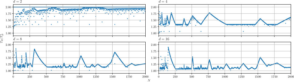
Figure 12: $T_{B}/T_{B}^{*}$ of generalized Kautz graph $\Pi_{d,N}$ up to $N=2000$. As can be seen, the BW runtime of $\Pi_{d,N}$ is less than or equal to $2T_{B}^{*}$ at all times for $d=2,4,8,16$. In particular, the higher the degree is, the closer $T_{B}$ is to optimal. As for node latency, Theorem 21 shows that $T_{L}\leq T_{L}^{*}(N,d)+\alpha$.

Generalized Kautz graph [33, 15] is a low-$T_{L}$ unidirectional topology that can be constructed for every $N$ and $d$.

Definition 16 (Generalized Kautz Graph).

The $\Pi_{d,m}$ digraph has the set of integers modulo $m$ as vertex set. Its arc set $A$ is defined as follows:

$$A=\{(x,y)\ |\ y\equiv-dx-a,1\leq a\leq d\}.$$

If $m=d^{n+1}+d^{n}$, then $\Pi_{d,m}=K(d,n)$, where $K(d,n)$ is the Kautz graph $L^{n}(K_{d+1})$.

We apply BFB schedule generation to generalized Kautz graph. The resulting schedule is not always Moore optimal, but the following theorem shows that it is at most one $\alpha$ away from Moore optimality, i.e., $T_{L}\leq T_{L}^{*}(N,d)+\alpha$:

Theorem 21.

Suppose $D(\Pi_{d,m})=k$, then $m>M_{d,k-2}$.

Remember Moore optimality is stricter than node latency optimality, so it is possible that generalized Kautz graph is node latency optimal. The special case, Kautz graph $K(d,n)$, is always Moore optimal and is, in fact, the largest known digraph in degree/diamter problem for any degree $d>2$ [50].

As for BW performance, from Figure 12, one can see that generalized Kautz graph is also close to BW optimality, especially at higher degrees.

E.3 Distance-Regular Graph

In graph theory, distance-regular graphs are a family of highly symmetric undirected graphs. We can show that there exists a BW-optimal BFB schedule for any distance-regular graph, and thus LP (3) can always generate one. We borrow the following definition from [13]:

Definition 17 (Distance-Regular Graph).

A connected graph $G$ is distance-regular if for any vertices $x,y\in V_{G}$ and integers $i,j$, the number of vertices at distance $i$ from $x$ and distance $j$ from $y$ depends only on $i,j$ and $d(x,y)$.

In other words, there exists a constant $s^{h}_{i,j}$ for every $h,i,j$ such that $s^{h}_{i,j}=|N_{i}(x)\cap N_{j}(y)|$ whenever $x,y\in V_{G}$ satisfy $d(x,y)=h$. Thus, we can apply Theorem 18 with $N_{x}=s^{0}_{x,x}$, $a_{x}=s^{1}_{x,x-1}$, and $b_{x}=s^{x}_{1,x-1}$.

The significance of distance-regular graph is not only about BW optimality. Many of distance-regular graphs have low diameters, so their schedules are not only BW-optimal but also close to, and in some cases exactly, Moore optimal. Table 7 gives examples of distance-regular graphs at $d=4$. In addition, many of the base graphs mentioned in this paper are also distance-regular like complete bipartite graphs (Figure 1) and Hamming graphs. One can refer to [2] for a repository of distance-regular graphs.

Graph Name	$N$	$T_{L}$	$T_{L}^{*}$	$T_{L}\!-\!T_{L}^{*}$	$T_{L}^{**}$	$T_{L}\!-\!T_{L}^{**}$
Octahedron J(4,2)	6	2	2	0	2	0
Paley graph P9$\cong$H(2,3)	9	2	2	0	2	0
K5,5-I	10	3	2	1	2	1
Distance-3 graph of Heawood graph	14	3	2	1	2	1
Line graph of Petersen graph	15	3	2	1	2	1
4-cube Q4$\cong$H(4,2)	16	4	2	2	2	2
Line graph of Heawood graph	21	3	2	1	3	0
Incidence graph of PG(2,3)	26	3	3	0	3	0
Incidence graph of AG(2,4) minus a parallel class	32	4	3	1	3	1
Odd graph O4	35	3	3	0	3	0
Line graph of Tutte’s 8-cage	45	4	3	1	3	1
Doubled Odd Graph D(O4)	70	7	3	4	4	3
Incidence graph of GQ(3,3)	80	4	3	1	4	0
Line graph of Tutte’s 12-cage	189	6	4	2	5	1
Incidence graph of GH(3,3)	728	6	5	1	6	0

Table 7: Examples of distance-regular graphs at $d=4$ [2]. $T_{L}^{**}$ is the bidirectional Moore optimality.

E.4 Circulant Graph

Circulant graph is a well-studied topology in both graph theory and network design. Many popular network topologies like shifted ring, chordal ring, and loop network are either part of or closely related to circulant graphs. The definition of circulant graph is as follows:

Definition 18.

The circulant graph $C(n,\{a_{1},\dots,a_{k}\})$ is a bidirectional graph with vertex set $\{0,1,\dots,n-1\}$ and each node $i$ is adjacent to nodes $i\pm a_{1},\dots,i\pm a_{k}\pmod{n}$.

Note that in this paper, we only consider connected circulant graphs, and $C(n,\{a_{1},\dots,a_{k}\})$ is connected if and only if $\gcd(n,a_{1},\dots,a_{k})=1$ [51, 47]. It is easy to see that $C(n,\{a_{1},\dots,a_{k}\})$ is an $n$-node $2k$-regular topology.

We have found that the BFB schedule generation seems to give BW-optimal schedules for all circulant graphs. In particular, we have the following conjecture:

Conjecture 1.

For any circulant graph $C(n,\{a_{1},\dots,a_{k}\})$, there exists a BW-optimal BFB schedule.

While we leave a complete proof or disproof of this conjecture for future work, we have proved the conjecture holds when $k=2$, which corresponds to the graph having degree 4.

Circulant graph revolutionized our Pareto frontier of topologies since it can be constructed for every $N$ and even value $d$. It can provide a BW-optimal topology if our expansion techniques fail to produce one at some $N$ and $d$. Since all circulant graphs seem to be BW-optimal, the question is what choices of $a_{1},\dots,a_{k}$ result in minimum node latency, or equivalently, minimum diameter for a given $n$ and $k$. While this remains largely an open question in graph theory [51], the case of $k=2$ has been solved in [17]:

Theorem 22.

Given $n\!>\!6$ and $m\!=\!\lceil(-\!1\!+\!\sqrt{2n\!-\!1})\!/\!2\rceil$, circulant graph $C(n,\{m,m\!+\!1\})$ has a diameter equal to $m$, which is the minimum diameter over all circulant graphs $C(n,\{a_{1},a_{2}\})$.

We can certainly use multiedge to apply this construction for any even degree that is $\geq 4$. The resulting topology has $\Theta(\sqrt{N})$ diameter, which is a significant improvement in terms of node latency when BW optimality is required. Previously, the only topology that is known to be BW-optimal for any $N$ and $d$ is ring, which has $\Theta(N)$ diameter.

Appendix F Unidirectional to Bidirectional

While this paper focuses on unidirectional topologies, many of the techniques can be conveniently applied to bidirectional topologies as well. For example, BFB schedule generation, degree expansion, and Cartesian product can all be used on bidirectional topologies by replacing each bidirectional edge with two opposite unidirectional edges. The resulting degree expanded and Cartesian product topologies still have unidirectional edges in opposite pairs. Although line graph expansion only works within unidirectional topologies, there is a way to convert unidirectional topology and schedule to bidirectional ones with zero performance sacrifice. In this section, we will show how to convert a reverse-symmetric $d$-regular unidirectional topology $G$ and its allgather schedule $A$ to a $2d$-regular bidirectional topology $G^{\prime}$ and its schedule $A^{\prime}$ such that $T_{L}(A)\!=\!T_{L}(A^{\prime})$ and $T_{B}(A)\!=\!T_{B}(A^{\prime})$.

Let $g\!:\!V_{G}\!\to\!V_{G^{T}}$ be the isomorphism from $G$ to $G^{T}$, then it is trivial to see that $g(A)$ (see Definition 9) is an allgather schedule for $G^{T}$. Observe that $G^{\prime}\!=\!G\cup G^{T}$ is a $2d$-regular bidirectional topology. Consider both $A$ and $g(A)$ as allgather schedules for bidirectional topology $G^{\prime}$. Schedules $A$ and $g(A)$ use disjoint sets of edges, because they use opposite directions. Thus, we can divide each shard into two halves. Let one half follow schedule $A$ and the other half follow $g(A)$. Let such a schedule be $A^{\prime}$.

It is trivial to see that $T_{L}(A)\!=\!T_{L}(A^{\prime})$. As for $T_{B}(A)\!=\!T_{B}(A^{\prime})$, it follows the fact that the total data size is halved for each of $A$ and $g(A)$, but the bandwidth per edge is also halved due to the doubling of degree. Note that if $A$ is BW-optimal, then $A^{\prime}$ is BW-optimal; however, $A^{\prime}$ is not necessarily Moore optimal if $A$ is Moore optimal.

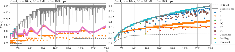
Figure 13: The minimum allreduce runtimes at different $N$ for $d=4$, $\alpha=10\mu s$, and $M/B=1\textnormal{MB}/100\textnormal{Gbps},100\textnormal{MB}/100\textnormal{Gbps}$. “L”, “P”, and “C” stand for line graph, Cartesian power, and Cartesian product (of different graphs) respectively. For example, “LC” means the runtime is achieved by a topology whose construction involves line graph expansion and Cartesian product. “GenKautz”, “DistReg”, and “Circulant” stand for generalized Kautz graph (§E.2), distance regular graph (§E.3), and circulant graph (§E.4) respectively. The figures also show the best bidirectional topology known at different $N$s. Degree expansion does not show up due to target $d=4$ being relatively small.

Appendix G Pareto-Efficiency Analysis

There could exist multiple Pareto-efficient topologies at given $N$ and $d$. For different $\alpha$ and $M/B$, the Pareto-efficient topology with minimum allreduce runtime is also different. To see how $N$ affects the best choice of topologies, we use topology finder (§5.4) to generate Pareto-efficient topologies at $d=4$ for $N$ up to 2000 and pick the best one based on specific values of $\alpha$ and $M/B$.

Figure 13 shows two examples of such analysis. At $M=1$MB, node latency is more important than BW runtime. Thus, we see that generalized Kautz graph is the most popular one, being the best topology at many $N$s. On the contrary, at $M=100$MB, BW performance becomes the dominant factor, and thus circulant graph becomes the most popular one. Line graphs are also popular in both settings; however, line graph expansion requires target $N$ to be divisible by some power of $d$, so it does not work for any $N$.

Appendix H Cost Model Validation

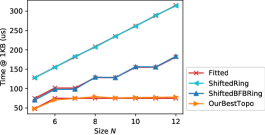
(a) Node Latency $T_{L}$ (Relative error: avg 1.71%, max 6.21%)

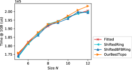
(b) BW Runtime $T_{B}$ (Relative error: avg 0.47%, max 1.32%)

Figure 14: Linear regression results.

Despite the wide acceptance of $\alpha$-$\beta$ cost model by previous literature [31, 21, 19, 60, 58], we also did a linear regression analysis to verify the cost model on our testbed. In particular, we want to verify that (1) node latency follows $T_{L}=\alpha\cdot x+\epsilon$ and (2) BW runtime follows $T_{B}=\frac{M}{B}\cdot y$, where $x$ and $y$ are the number of comm steps and bandwidth factor respectively ($y=2\cdot\frac{N-1}{N}$ if BW-optimal). $\epsilon$ is the constant latency including time costs such as GPU kernel launching. Here, we use linear regression to derive the values of $\alpha$, $\epsilon$, and $1/B$, and compute the relative errors between observed runtimes and fitted runtimes. We fit the allreduce runtimes at 1KB to the node latency, since BW runtime is negligible at such a small $M$. Similarly, we fit runtimes at 1GB to the BW runtime, since node latency is negligible at such a large $M$.

Figure 14(a) and 14(b) show our results of linear regression analysis to verify our cost model. For node latency, we obtain estimates $\alpha\!\approx\!13.33$us and $\epsilon\!\approx\!21.60$us with low errors (average and maximum relative errors of 1.71% and 6.21% respectively). As one can see from Figure 14(a), ShiftedRing and ShiftedBFBRing have a straight and a stair-step shape of runtime growth respectively, which match the expected numbers of comm steps $2(N-1)$ and $2\lfloor N/2\rfloor$ respectively. For BW runtime, we get an estimate $1/B\!\approx\!1.018\!\times\!10^{-4}$us/byte or $B\!\approx\!79$Gbps with low errors (average and maximum relative errors of 0.47% and 1.32% respectively). As one can see from Figure 14(b), all three topologies follow the fitted curve $2\frac{\text{1GB}}{B}\cdot\frac{N-1}{N}\!=\!2T^{*}_{B}(N)$ since they are all BW-optimal. However, there is a gap between $B\!\approx\!79$Gbps and the hardware theoretical bandwidth 4x25Gbps$=$100Gbps. Besides inevitable loss of bandwidth in actual communication, the gap can also be explained by the fact that computational cost of reduction also accounts for part of $1/B$ as discussed in §B.4.

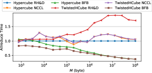
Figure 15: Comparing switch allreduce solutions (recursive halving & doubling (RH&D), NCCL) against BFB schedule on hypercube and twisted hypercube on $N\!=\!8,d\!=\!3$ testbed. The runtimes are normalized by the runtime of recursive halving & doubling on hypercube.

Appendix I Comparison Against Switch Solutions

NCCL [5] and recursive halving & doubling (RH&D) are widely adopted collective communication solutions on switch networks. We assess the schedule performance of BFB against these solutions over two direct-connect 8-node topologies: hypercube and twisted hypercube [27]. Hypercube is widely used in HPC settings, and its connections perfectly match the communication pattern of RH&D. Twisted hypercube is a variant of hypercube with a lower diameter.

Figure 15 compares the baselines against our BFB schedule when run over either hypercube or twisted hypercube with $N\!=\!8$, $d\!=\!3$ on the testbed. At small $M$, all schedules and topologies perform roughly the same, except BFB can take advantage of the lower diameter of twisted hypercube and achieve $\sim\!\!20\%$ lower runtime. At large $M$, because BFB achieves BW optimality on both topologies, it performs even better with 60% lower runtime. RH&D and NCCL perform poorly as $M$ grows because they cannot utilize all $d\!=\!3$ links simultaneously. At every comm step of RH&D, a node only communicates with one of the three neighbors, utilizing at most $1/3$ of the total bandwidth (similarly with NCCL). Also, because the schedule is not matched to the twisted hypercube, some nodes communicate with nodes multiple hops away, occupying more link capacities and causing congestion.

In summary, BFB schedules can fully exploit direct-connect topologies and provide better performance than solutions designed for switch networks.

Appendix J Proofs

See 1

Proof.

Let $v^{\prime}\!v,uw$ be arbitrary two distinct vertices in $L(G)$. We want to show there exists a sequence in $A_{L(G)}$ going from $v^{\prime}\!v$ to $uw$ like in Definition 6 for any $x\!\in\!S$. If $u\!=\!v$, then $((v^{\prime}\!v,S),(v^{\prime}\!v,uw),1)$ at the first comm step suffices. If $u\!\neq\!v$, because $A_{G}$ is allgather, there exists a sequence in $A_{G}$:

$$((v,C_{1}),(v,w_{1}),t_{1}),((v,C_{2}),(w_{1},w_{2}),t_{2}),\dots{\\ }((v,C_{n}),(w_{n-1},u),t_{n}),$$

where $t_{1}<t_{2}<\dots<t_{n}$ and $x\!\in\!C_{1}\cap C_{2}\cap\dots\cap C_{n}$. Thus, by Definition 2, there exists a sequence in $A_{L(G)}$:

$$((v^{\prime}\!v,S),(v^{\prime}\!v,vw_{1}),1),((v^{\prime}\!v,C_{1}),(vw_{1},w_{1}w_{2}),t_{1}+1),\dots{\\ }((v^{\prime}\!v,C_{n}),(w_{n-1}u,uw),t_{n}+1),$$

as desired. The new algorithm $(L(G),A_{L(G)})$ has $dM$ total data length, because the number of nodes has grown $d$-fold while the size of a shard remains the same.

As for $T_{L}(A_{L(G)})$ and $T_{B}(A_{L(G)})$, equality (1) trivially follows the Definition 2. Let $[A_{L(G)}]_{t}$ and $[A_{G}]_{t}$ be the subschedules of $A_{L(G)}$ and $A_{G}$ at comm step $t$. Given $v\!\in\!V_{G}$, because $G$ is $d$-regular, we have $|\{v^{\prime}\!v\ |\ v^{\prime}\!v\!\in\!V_{L(G)}\}|\!=\!|\{(v^{\prime},v)\ |\ (v^{\prime},v)\!\in\!E_{G}\}|\!=\!d$. Given any edge $(uw,ww^{\prime})$ and $t$, there are at most $d$ number of $((v^{\prime}\!v,C),(uw,ww^{\prime}),t+1)\!\in\!A_{L(G)}$ for each $((v,C),(u,w),t)\!\in\!A_{G}$ by Definition 2. Thus, given $(uw,ww^{\prime})$,

$$\sum_{((v^{\prime}\!v,C),(uw,ww^{\prime}))\in[A_{L(G)}]_{t+1}}|C|\leq\sum_{((v,C),(u,w))\in[A_{G}]_{t}}d\cdot|C|.$$

It follows that $T_{B}([A_{L(G)}]_{t+1},dM,B)\leq d\cdot T_{B}([A_{G}]_{t},M,B)$ and hence $\sum_{t=2}^{t_{\max}+1}T_{B}([A_{L(G)}]_{t},dM,B)\leq d\cdot T_{B}(A_{G},M,B)$. For the first comm step, we have

$$T_{B}([A_{L(G)}]_{1},dM,B)=\frac{|S|}{B/d}=\frac{M/N}{B/d}.$$

Assuming $T_{B}(A_{G},M,B)\!=\!\tau(M/B)$ for some constant $\tau$, we have $d\cdot T_{B}(A_{G},M,B)\!=\!T_{B}(A_{G},dM,B)$. It follows that

$$T_{B}(A_{L(G)},dM,B)=\sum_{t=1}^{t_{\max}+1}T_{B}([A_{L(G)}]_{t},dM,B)\\ \leq\frac{M/N}{B/d}+d\cdot T_{B}(A_{G},M,B)=T_{B}(A_{G},dM,B)+\frac{dM}{B}\cdot\frac{1}{N}.$$

Replacing $dM$ by $M$ gives (2) as desired. ∎

See 1.2

See 2

Proof.

If $(G,A_{G})$ is BW-optimal, then $T_{B}(A_{G})\!=\!\frac{M}{B}\cdot\frac{N-1}{N}$ and

$$T_{B}(A_{L^{n}(G)})\leq\frac{M}{B}\left[1+\frac{1}{d-1}\left(\frac{1}{N}-\frac{d}{d^{n}N}\right)\right].$$ (14)

It is trivial to see that $(\ref{eq:bwoptlinenbw})/T_{B}^{*}(d^{n}N)\nearrow 1+[(d-1)N]^{-1}$ as $n\to\infty$. ∎

See 3

Proof.

Suppose $(G,A)$ is a reduce-scatter algorithm. For arbitrary $x\!\in\!S$ and distinct $u,v\!\in\!V_{G}$, there exists a sequence of tuples in $A$:

$$((v,C_{1}),(u,w_{1}),t_{1}),((v,C_{2}),(w_{1},w_{2}),t_{2}),\dots{\\ }((v,C_{n}),(w_{n-1},v),t_{n}),$$

where $t_{1}<t_{2}<\dots<t_{n}$ and $x\!\in\!C_{1}\cap C_{2}\cap\dots\cap C_{n}$. It follows that there exists a sequence of tuples in $A^{T}$:

$$((v,C_{n}),(v,w_{n-1}),t_{n}^{\prime}),\dots{\\ }((v,C_{2}),(w_{2},w_{1}),t_{2}^{\prime}),((v,C_{1}),(w_{1},u),t_{1}^{\prime}).$$

where $t_{i}^{\prime}\!=\!t_{\max}-t_{i}+1$, so $t_{n}^{\prime}<\dots<t_{2}^{\prime}<t_{1}^{\prime}$. Since $u,v,x$ are abitrary, $A^{T}$ is an allgather schedule on $G^{T}$. One can similarly show that if $(G,A)$ is an allgather algorithm, then $(G^{T},A^{T})$ is a reduce-scatter algorithm. ∎

See 3.1 See 3.2

See 4

Proof.

By definition of $f(A^{T})$,

$$((f(v),C),(f(w),f(u)), t_{\max}-t+1)\in f(A^{T})$$

$$\Leftrightarrow\ ((v,C),(w,u),t_{\max}-t+1)\in A^{T}$$

$$\Leftrightarrow\ ((v,C),(u,w),t)\in A.$$

Note that $(u,w)\!\in\!E_{G}\Leftrightarrow(w,u)\!\in\!E_{G^{T}}\Leftrightarrow(f(w),f(u))\!\in\!E_{G}$, so $f(A^{T})$ is a valid schedule for $G$.

Suppose $(G,A)$ is a reduce-scatter algorithm. For any $x\!\in\!S$ and distinct $u,v\!\in\!V_{G}$, there exists a sequence of tuples in $A$:

$$((v,C_{1}),(u,w_{1}),t_{1}),((v,C_{2}),(w_{1},w_{2}),t_{2}),\dots{\\ }((v,C_{n}),(w_{n-1},v),t_{n}),$$

where $t_{1}<t_{2}<\dots<t_{n}$ and $x\!\in\!C_{1}\cap C_{2}\cap\dots\cap C_{n}$. It follows that there exists a sequence of tuples in $f(A^{T})$:

$$((f(v),C_{n}),(f(v),f(w_{n-1})),t_{n}^{\prime}),$$

$$((f(v),C_{n-1}),(f(w_{n-1}),f(w_{n-2})),t_{n-1}^{\prime}),$$

$$\vdots$$

$$((f(v),C_{1}),(f(w_{1}),f(u)),t_{1}^{\prime}),$$

where $t_{i}^{\prime}\!=\!t_{\max}-t_{i}+1$, and $x\!\in\!C_{n}\cap C_{n-1}\cap\dots\cap C_{1}$. Because $f$ is a bijection, $(G,f(A^{T}))$ is an allgather algorithm. $T_{L}(A)\!=\!T_{L}(f(A^{T}))$ and $T_{B}(A)\!=\!T_{B}(f(A^{T}))$ are trivial, and one can similarly prove that if $(G,A)$ is an allgather algorithm, then $(G,f(A^{T}))$ is a reduce-scatter algorithm. ∎

See 5

Proof.

The proof is mentioned in text. ∎

See 5.1

See 6

Proof.

The proof is mentioned in text. ∎

See 6.1

See 7

Proof.

If $T_{B}(A)\!=\!T^{*}_{B}(N)\!=\!\frac{M}{B}\cdot\frac{N-1}{N}$, then the amount of data received by each vertex must be equal to $M\cdot\frac{N-1}{N}$, and the ingress bandwidth $B$ must be fully utilized. If condition 1 does not hold, then some link $(w,u)$ is not fully utilized. If condition 2 does not hold, then the amount of data received by some node is greater than $M\cdot\frac{N-1}{N}$.

If both 1 and 2 hold, then every vertex receives exactly $M\cdot\frac{N-1}{N}$ in total and bandwidth are fully utilized. Thus, $T_{B}(A)\!=\!T^{*}_{B}(N)$ and $(G,A)$ is BW-optimal. ∎

See 8

Proof.

At any comm step $t$, suppose the BW runtime is $T_{B}(A_{t})\!=\!\frac{M}{B}\cdot y_{t}$. It follows at comm step $t$, the amount of data each node receives is at most $B\cdot T_{B}(A_{t})\!=\!M\cdot y_{t}$, so $T_{C}(A_{t})\leq M\cdot\gamma\cdot y_{t}$. The theorem trivially follows $y\!=\!\sum_{t}y_{t}$. ∎

See 8.1

See 9

Proof.

Suppose $T_{L}(A_{G})\!=\!\alpha k$. Thus, $(G,A_{G})$ is Moore optimal if and only if

$$N>M_{d,k-1}=\sum_{i=0}^{k-1}d^{i}=\frac{d^{k}}{d-1}-\frac{1}{d-1}.$$ (15)

$(L^{n}(G),A_{L^{n}(G)})$ is Moore optimal if and only if

$$d^{n}N>M_{d,k+n-1}\ \Leftrightarrow\ N>\frac{d^{k}}{d-1}-\frac{1}{d^{n}(d-1)}.$$ (16)

Because $\eqref{eq:resultnodeopt}-\eqref{eq:basenodeopt}<1$ and (15) is an integer, (15) and (16) are equivalent. ∎

See 10

Proof.

It is trivial to see that $A_{L(G)}$ is a BFB allgather schedule on $L(G)$ by property (2) in §5.1. For the sake of contradiction, suppose there exists a BFB schedule $A^{\prime}_{L(G)}$ that $T_{B}(A^{\prime}_{L(G)})<T_{B}(A_{G})+\frac{M}{B}\cdot\frac{1}{N}$. Let $x_{v^{\prime}\!v,(wu,uu^{\prime}),t}^{*}$s be the solution of BFB LP (3) corresponding to $A^{\prime}_{L(G)}$. We build a schedule $A^{\prime}_{G}$ by constructing a solution of (3) such that

$$x_{v,(w,u),t}=\frac{1}{d}\sum_{v^{\prime}\in N^{-}(v)}x_{v^{\prime}\!v,(wu,uu^{\prime}),t+1}^{*},$$

where $u^{\prime}\!\in\!N^{+}(u)\setminus\{v\}$ is arbitrary. To verify the construction is a valid solution, given any $u\!\in\!V_{G}$ and $v\!\in\!N^{-}_{t}(w)$, the equality of (3) follows:

$$\sum_{w}x_{v,(w,u),t}=\frac{1}{d}\sum_{v^{\prime}}\sum_{w}x_{v^{\prime}\!v,(wu,uu^{\prime}),t+1}^{*}\\ =\frac{1}{d}\sum_{v^{\prime}}\sum_{wu}x_{v^{\prime}\!v,(wu,uu^{\prime}),t+1}^{*}=\frac{1}{d}\sum_{v^{\prime}}1=\frac{1}{d}\cdot d=1.$$

The third equality follows the equality constraint in (3). Now, given $(w,u)\!\in\!E_{G}$, observe that

$$\sum_{v}x_{v,(w,u),t}=\frac{1}{d}\sum_{v}\sum_{v^{\prime}}x_{v^{\prime}\!v,(wu,uu^{\prime}),t+1}^{*}\\ =\frac{1}{d}\sum_{v^{\prime}\!v}x_{v^{\prime}\!v,(wu,uu^{\prime}),t+1}^{*}\leq\frac{1}{d}U_{uu^{\prime},t+1}.$$

Thus, $U_{u,t}\!=\!\max_{w}\sum_{v}x_{v,(w,u),t}\!\leq\!\frac{1}{d}U_{uu^{\prime},t+1}$ and hence

$$\max_{u\in V_{G}}U_{u,t}\leq\frac{1}{d}\max_{uu^{\prime}\in V_{L(G)}}U_{uu^{\prime},t+1}.$$

By (4), we have

$$T_{B}(A^{\prime}_{G})\leq T_{B}(A^{\prime}_{L(G)})-\frac{M/(dN)}{B/d}\\ =T_{B}(A^{\prime}_{L(G)})-\frac{M}{B}\cdot\frac{1}{N}<T_{B}(A_{G}),$$

contradicting $A_{G}$ being the optimal BFB schedule. Thus, combined with inequality (2), we have proven $A_{L(G)}$ being optimal as well as the equality (7). ∎

See 10.1

See 11

Proof.

Let $u_{i},v_{j}$ be arbitrary two distinct vertices in $G*n$. Suppose $u\!\neq\!v$ in $G$, then for any $x\!\in\!S$, there exists a sequence in $A_{G}$:

$$((v,C_{1}),(v,w^{(1)}),t_{1}),((v,C_{2}),(w^{(1)},w^{(2)}),t_{2}),\dots{\\ }((v,C_{n}),(w^{(n-1)},u),t_{n}),$$

where $t_{1}<t_{2}<\dots<t_{n}$ and $x\!\in\!C_{1}\cap C_{2}\cap\dots\cap C_{n}$. By Definition 4, there exists a sequence in $A_{G*n}$:

$$((v_{j},C_{1}),(v_{j},w_{j}^{(1)}),t_{1}),((v_{j},C_{2}),(w_{j}^{(1)},w_{j}^{(2)}),t_{2}),\dots{\\ }((v_{j},C_{n}),(w_{j}^{(n-1)},u_{i}),t_{n}),$$

as desired. Now, suppose $u\!=\!v$ in $G$. By previous proof, the shard of $v_{j}$ reaches every in-neighbor $u^{\prime}_{\alpha}$ of $u_{i}$ by the end of comm step $t_{\max}$ since $u^{\prime}\!\neq\!v$. Then, the last comm step $t_{\max}+1$ added in step 2 of Definition 4 delivers the shard to $u_{i}$ with each edge $(u^{\prime}_{\alpha},u_{i})$ delivering $1/nd$ of a shard. Thus, $A_{G*n}$ is a complete allgather.

In step 1 of Definition 4, we have $T_{B}([A_{G*n}]_{t},nM,nB)\!=\!T_{B}([A_{G}]_{t},M,B)$ and hence $\sum_{t=1}^{t_{\max}}T_{B}([A_{G*n}]_{t},nM,nB)\!=\!T_{B}(A_{G},M,B)$. The $nM$ and $nB$ are due to the fact that both the number of nodes and degree have grown $n$-fold. Thus,

$$T_{B}(A_{G*n}, M,B)=T_{B}(A_{G*n},nM,nB)$$

$$=T_{B}(A_{G},M,B)+T_{B}([A_{G*n}]_{t_{\max}+1},nM,nB)$$

$$=T_{B}(A_{G},M,B)+(n-1)\cdot\frac{(nM)/(nN)}{nd}\cdot\frac{1}{nB/(nd)}$$

$$=T_{B}(A_{G},M,B)+\frac{M}{B}\cdot\frac{n-1}{nN}.$$

The first equality follows the assumption that $T_{B}(A_{G},M,B)\!=\!\tau(M/B)$ for some constant $\tau$. ∎

See 11.1

See 12

Proof.

We will show that $A^{(1)}$ is a valid allgather schedule. Since $A^{(i)}$s are simply starting at different dimensions, this also shows that $A^{(i)}$s and hence $A_{G^{\square n}}$ are all valid allgather schedules for $G^{\square n}$.

Let $\mathbf{u}$ be arbitrary vertex in $G^{\square n}$. For any $x\!\in\!S$, we will show that schedule $A^{(1)}$ broadcasts $x$ from $\mathbf{u}$ to all vertices in $G^{\square n}$. At $j\!=\!1$, $A^{(1)}$ performs an allgather over vertices $\{(v_{1},\mathbf{u}[2\!:\!n])\ |\ v_{1}\!\in\!V_{G}\}$ which induce a subgraph of $G^{\square n}$ isomorphic to $G$. Thus, $x$ has been broadcast to all vertices in $\{(v_{1},\mathbf{u}[2\!:\!n])\ |\ v_{1}\!\in\!V_{G}\}$. At $j\!=\!2$, $A^{(1)}$ performs an allgather over vertices $\{(v_{1},v_{2},\mathbf{u}[3\!:\!n])\ |\ v_{2}\!\in\!V_{G}\}$ for each $v_{1}$. By the end of $j\!=\!2$, $x$ has been broadcast to all vertices in $\{(v_{1},v_{2},\mathbf{u}[3\!:\!n])\ |\ v_{1},v_{2}\!\in\!V_{G}\}$. By the end of $j\!=\!n$, $x$ has been broadcast to all vertices in $\{\mathbf{v}\ |\ \mathbf{v}\!\in\!V_{G}^{n}\}\!=\!V_{G^{\square n}}$. Since $\mathbf{u}$ and $x$ are arbitrary, $A^{(1)}$ is a valid allgather schedule for $G^{\square n}$.

As for performance, (10) is trivial. To prove (11), observe that at each $j$ in $A^{(1)}$, allgather $A_{G}$ is performed with a data size $N^{j-1}M/n$ over the subgraph induced by $\{(\mathbf{y},v,\mathbf{z})\ |\ v\!\in\!V_{G}\}$ for each $\mathbf{y}\!\in\!V_{G}^{j-1},\mathbf{z}\!\in\!V_{G}^{n-j}$. The bandwidth of each node within the subgraph is $1/n$ of that in $G^{\square n}$. It follows that

$$T_{B}(A^{(1)},N^{n-1}M/n,nB) =\sum_{j=1}^{n}T_{B}(A_{G},N^{j-1}M/n,B)$$

$$=\sum_{j=1}^{n}\frac{N^{j-1}}{n}T_{B}(A_{G},M,B)$$

$$=\frac{N^{n}-1}{n(N-1)}T_{B}(A_{G},M,B).$$

Therefore,

$$T_{B}(A_{G^{\square n}},M,B) =\frac{n}{N^{n-1}}T_{B}(A_{G^{\square n}},N^{n-1}M,nB)$$

$$=\frac{n}{N^{n-1}}T_{B}(A^{(1)},N^{n-1}M/n,nB)$$

$$=\frac{n}{N^{n-1}}\cdot\frac{N^{n}-1}{n(N-1)}T_{B}(A_{G},M,B)$$

$$=T_{B}(A_{G},M,B)\cdot\frac{N}{N-1}\cdot\frac{N^{n}-1}{N^{n}}.$$

∎

See 12.1

See 13

Proof.

To prove the theorem, it is sufficient to show that if $G_{1}$ and $G_{2}$ have BW-optimal BFB schedules, then $G_{1}\square G_{2}$ has a BW-optimal BFB schedule. By Theorem 16, let $x^{*}_{v_{1},(w_{1},u_{1}),t_{1}}$s and $x^{*}_{v_{2},(w_{2},u_{2}),t_{2}}$s be the solutions of (3) on $G_{1}$ and $G_{2}$ respectively. Let $\mathbf{u}\!=\!(u_{1},u_{2}),\mathbf{v}\!=\!(v_{1},v_{2})$. Define $r\!\in\![0,1]$, which we will decide later. We construct a solution of (3) for $G_{1}\square G_{2}$ such that:

$$x_{\mathbf{v},((w_{1},u_{2}),\mathbf{u}),t_{1}+t_{2}} =\begin{cases}r\cdot x^{*}_{v_{1},(w_{1},u_{1}),t_{1}}&\text{if $u_{2}\neq v_{2}$,}\\ x^{*}_{v_{1},(w_{1},u_{1}),t_{1}}&\text{if $u_{2}=v_{2}$,}\end{cases}$$ (17)

$$x_{\mathbf{v},((u_{1},w_{2}),\mathbf{u}),t_{1}+t_{2}} =\begin{cases}(1-r)\cdot x^{*}_{v_{2},(w_{2},u_{2}),t_{2}}&\text{if $u_{1}\neq v_{1}$,}\\ x^{*}_{v_{2},(w_{2},u_{2}),t_{2}}&\text{if $u_{1}=v_{1}$.}\end{cases}$$

First of all, because $d_{G_{1}\square G_{2}}(\mathbf{v},\mathbf{u})\!=\!d_{G_{1}}(v_{1},u_{1})+d_{G_{2}}(v_{2},u_{2})$, it is easy to verify that (17) gives a BFB schedule. In addition, for any distinct $\mathbf{u},\mathbf{v}\!\in\!G_{1}\square G_{2}$ with $u_{1}\!\neq\!v_{1}$ and $u_{2}\!\neq\!v_{2}$,

$$\sum_{\mathbf{w}}x_{\mathbf{v},(\mathbf{w},\mathbf{u}),t_{1}+t_{2}} =r\sum_{w_{1}}x^{*}_{v_{1},(w_{1},u_{1}),t_{1}}+(1-r)\sum_{w_{2}}x^{*}_{v_{2},(w_{2},u_{2}),t_{2}}$$

$$=r+(1-r)$$

$$=1$$

satisfying the equality in (3). The $u_{1}\!=\!v_{1}$ or $u_{2}\!=\!v_{2}$ case is trivial. Because $G_{1}$ and $G_{2}$ have BW-optimal BFB schedule, by Theorem 17, for any $(w_{1},u_{1})\!\in\!E_{G_{1}}$,

$$\sum_{v_{1}\in N^{-G_{1}}_{t}(u_{1})}x^{*}_{v_{1},(w_{1},u_{1}),t}=\frac{N^{-G_{1}}_{t}}{d_{1}},$$ (18)

where $N^{-G_{1}}_{t}(u_{1})$ is $N^{-}_{t}(u_{1})$ in $G_{1}$. Define $N^{-G_{1}\square G_{2}}_{t_{1},t_{2}}(\mathbf{u})\!=\!N_{t_{1}}^{-G_{1}}(u_{1})\times N_{t_{2}}^{-G_{2}}(u_{2})$, then it holds that

$$N_{t}^{-G_{1}\square G_{2}}(\mathbf{u})=\bigcup_{t_{1}=0}^{t}N^{-G_{1}\square G_{2}}_{t_{1},t-t_{1}}(\mathbf{u})\\ =N_{t}^{-G_{1}}(u_{1})\times\{u_{2}\}\cup\{u_{1}\}\times N_{t}^{-G_{2}}(u_{2})\cup\bigcup_{t_{1}=1}^{t-1}N^{-G_{1}\square G_{2}}_{t_{1},t-t_{1}}(\mathbf{u}).$$

Thus, (18) gives

$$\sum_{\mathbf{v}\in N_{t}^{-G_{1}\square G_{2}}(\mathbf{u})}x_{\mathbf{v},((w_{1},u_{2}),\mathbf{u}),t}=\frac{N^{-G_{1}}_{t}}{d_{1}}+r\sum_{t_{1}=1}^{t-1}\frac{N^{-G_{1}}_{t_{1}}N^{-G_{2}}_{t-t_{1}}}{d_{1}}.$$ (19)

for any $((w_{1},u_{2}),\mathbf{u})\!\in\!E_{G_{1}\square G_{2}}$. For $G_{2}$, one can similarly get

$$\sum_{\mathbf{v}\in N_{t}^{-G_{1}\square G_{2}}(\mathbf{u})}x_{\mathbf{v},((u_{1},w_{2}),\mathbf{u}),t}=\frac{N^{-G_{2}}_{t}}{d_{2}}+(1-r)\sum_{t_{2}=1}^{t-1}\frac{N^{-G_{1}}_{t-t_{2}}N^{-G_{2}}_{t_{2}}}{d_{2}}.$$ (20)

The value of $r$ is the solution to $(\ref{eq:cartesianlink1})\!=\!(\ref{eq:cartesianlink2})$:

$$\frac{N^{-G_{1}}_{t}}{d_{1}}+r\sum_{t_{1}=1}^{t-1}\frac{N^{-G_{1}}_{t_{1}}N^{-G_{2}}_{t-t_{1}}}{d_{1}}=\frac{N^{-G_{2}}_{t}}{d_{2}}+(1-r)\sum_{t_{2}=1}^{t-1}\frac{N^{-G_{1}}_{t-t_{2}}N^{-G_{2}}_{t_{2}}}{d_{2}}.$$

To see there is always a solution $r\!\in\![0,1]$, we have $N^{-G_{1}}_{t}\leq d_{1}\cdot N^{-G_{1}}_{t-1}$ and $N^{-G_{2}}_{t}\leq d_{2}\cdot N^{-G_{2}}_{t-1}$, so

$$\frac{N^{-G_{1}}_{t}}{d_{1}}-\frac{N^{-G_{2}}_{t}}{d_{2}}\leq\frac{N^{-G_{1}}_{t}}{d_{1}}\leq N^{-G_{1}}_{t-1}\leq\sum_{t_{2}=1}^{t-1}\frac{N^{-G_{1}}_{t-t_{2}}N^{-G_{2}}_{t_{2}}}{d_{2}},$$

$$\frac{N^{-G_{2}}_{t}}{d_{2}}-\frac{N^{-G_{1}}_{t}}{d_{1}}\leq\frac{N^{-G_{2}}_{t}}{d_{2}}\leq N^{-G_{2}}_{t-1}\leq\sum_{t_{1}=1}^{t-1}\frac{N^{-G_{1}}_{t_{1}}N^{-G_{2}}_{t-t_{1}}}{d_{1}}.$$

The last inequality follows that because $G_{2}$ is nontrivial simple digraph, $N^{-G_{2}}_{1}\!=\!d_{2}$ and hence $N^{-G_{1}}_{t-1}\!=\!N^{-G_{1}}_{t-1}N^{-G_{2}}_{1}/d_{2}$. Note that $a+rb\!=\!c+(1-r)d$ always has a solution $r\!\in\![0,1]$ if $a-c\leq d$ and $c-a\leq b$. With $(\ref{eq:cartesianlink1})\!=\!(\ref{eq:cartesianlink2})$, by Theorem 17, we have constructed a BW-optimal solution of (3) for $G_{1}\square G_{2}$. The theorem trivially follows by induction. ∎

See 14

Proof.

Let $v_{0},v_{k}$ be arbitrary two distinct vertices in $V_{G}$ with $d(v_{0},v_{k})\!=\!k$. For any $x\!\in\!S$, we want to show that there exists a path taking $x$ from $v_{0}$ to $v_{k}$. At comm step $k$, conditions 1 and 2 guarantee that there exists $v_{k-1}\!\in\!N^{-}(v_{k})$ and $((v_{0},C_{k}),(v_{k-1},v_{k}),k)\!\in\!A$ such that $d(v_{0},v_{k-1})\!=\!k-1$ and $x\!\in\!C_{k}$. At comm step $k-1$, similarly, it is guaranteed that there exists $v_{k-2}\!\in\!N^{-}(v_{k-1})$ and $((v_{0},C_{k-1}),(v_{k-2},v_{k-1}),k-1)\!\in\!A$ such that $d(v_{0},v_{k-2})\!=\!k-2$ and $x\!\in\!C_{k-1}$. Thus, we have a sequence of tuples in $A$:

$$((v_{0},C_{1}),(v_{0},v_{1}),1),((v_{0},C_{2}),(v_{1},v_{2}),2),\dots{\\ }((v_{0},C_{k}),(v_{k-1},v_{k}),k),$$

where $x\!\in\!C_{1}\cap C_{2}\cap\dots\cap C_{k}$ as desired. In the other direction, if condition 1 fails, then $A$ is not a BFB schedule; if condition 2 fails, then $A$ is not a valid allgather schedule. ∎

See 15

Proof.

The proof is trivial. ∎

See 16

Proof.

The proof is mentioned in text. ∎

See 17

Proof.

At comm step $t$, each vertex needs to receive shards from vertices in $N^{-}_{t}(u)$. By condition 1 of Theorem 7, each in-edge of vertex $u$ receives equal amount of data, so each in-edge receives $\frac{M}{N}|N^{-}_{t}(u)|/d$. In addition, condition 1 of Theorem 7 also forces every edge in $G$ receiving equal amount of data at any given comm step, so BW optimality is achieved if and only if $\frac{M}{N}|N^{-}_{t}(u)|/d\!=\!\frac{M}{N}|N^{-}_{t}(v)|/d\!=\!\frac{M}{N}N^{-}_{t}/d$ for all $u,v\!\in\!V_{G}$. Note that condition 2 of Theorem 7 is automatically satisfied. Thus, the conditions of Theorem 17 lead to Theorem 7, and vice versa. ∎

See 18

Proof.

It is easy to see $N_{x}=da_{x}/b_{x}$. Constant $N_{x}$s satisfy condition 1 of Theorem 17. As for 2 of Theorem 17, at comm step $t$, consider a BFB schedule such that for any $u,v,w\!\in\!V_{G}$ with $d(v,u)\!=\!d(v,w)+1\!=\!t$, node $w$ sends $1/b_{t}$ of $v$’s shard to $u$. Thus, $\sum_{((v,C),(w,u))\!\in\!A_{t}}|C|\!=\!\frac{M}{N}a_{t}/b_{t}\!=\!\frac{M}{N}N_{t}/d$. ∎

See 19

Proof.

Consider a flow network, where each $j_{a}$ is connected to each $p_{b}\!\in\!f(j_{a})$ with $\infty$ capacity. Source $s$ is connected to each $j_{a}$ with capacity 1, and each $p_{b}$ is connected to sink $t$ with capacity $m/d$. Thus, the workloads can be balanced if and only if the max flow is $m$. Given any subset $J$, consider the $s$-$t$ cut $(A,\bar{A})$ that $A\!=\!s+J+f(J)$. The cut has capacity $m-|J|+\frac{m}{d}|f(J)|$, which is less than $m$ if and only if the inequality is true. ∎

See 20

Proof.

For any $(w,u)$ at comm step $t$, since $|N^{-}_{t-1}(w)|\!\leq\!d^{t-1}$,

$$\sum_{v}y_{v,(w,u),t}<\sum_{v}1+y_{v,(w,u),t}^{\text{LP}}\leq d^{t-1}+\sum_{v}y_{v,(w,u),t}^{\text{LP}}.$$

Thus, we have $W_{u,t}\leq W_{u,t}^{\text{LP}}+d^{t-1}$. By (4),

$$T_{B}-T_{B}^{\text{OPT}}\leq T_{B}-T_{B}^{\text{LP}}\\ \leq\frac{M/N}{B/d}\cdot\frac{1}{P}\sum_{t=1}^{D(G)}d^{t-1}=\frac{M}{B}\cdot\frac{d(d^{D(G)}-1)}{(d-1)PN}.$$

Note that we need to divide (4) by $P$, because $y_{v,(w,u),t}\!\in\![0,P]$ in (12) while $x_{v,(w,u),t}\!\in\![0,1]$ in (3). If $G$ is Moore optimal (i.e., $N>M_{d,D(G)-1}$), it follows that

$$T_{B}-T_{B}^{\text{OPT}}<\frac{M}{B}\cdot\frac{d(d^{D(G)}-1)}{(d-1)PM_{d,D(G)-1}}=\frac{M}{B}\cdot\frac{d}{P}.$$

∎

See 21

Proof.

From [33], we know that $k\leq\lceil\log_{d}m\rceil$. Then,

$$m\geq d^{k-1}>\frac{d^{k-1}-1}{d-1}=M_{d,k-2}.$$

∎

See 22

Proof.

See [17]. ∎

Appendix K Supplementary Tables and Figures

DNN Model	OurBestTopo
alexnet	$L(\text{DBJMod}(2,4)^{\square 2})$
inception_v3	$L^{2}(\text{Diamond}^{\square 2})$
resnet18	$L^{2}(\text{Diamond}^{\square 2})$
resnet50	$L^{2}(\text{Diamond}^{\square 2})$
resnext50_32x4d	$L^{2}(\text{Diamond}^{\square 2})$
shufflenet_v2_x2_0	$L^{3}(C(16,\{3,4\}))$
squeezenet1_1	$L^{3}(C(16,\{3,4\}))$
vgg16	$L(\text{DBJMod}(2,4)^{\square 2})$
vgg19	$L(\text{DBJMod}(2,4)^{\square 2})$
bert	$L(\text{DBJMod}(2,4)^{\square 2})$
gpt2	$L(\text{DBJMod}(2,4)^{\square 2})$

Table 8: The topology used for each DNN model in the training simulation of Figure 8(b).

Figure 16: Diamond Topology $(N=8,d=2)$.

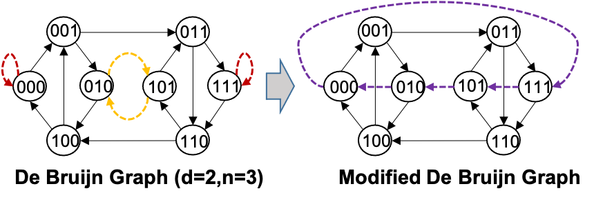
Figure 17: An Example of Modified de Bruijn Graph $(N=8,d=2)$. The modification rewires the self loops and 2-cycles in de Bruijn graph to form a single long cycle without violating degree constraint.

Topology	Symbol	Degree	Size	Reverse- Symmetric	Bandwidth Optimal	Moore Optimal	BFB Schedule	Self-Loop	MultiEdge
Complete	$K_{m}$	$m-1$	$m$	✓	✓	✓	✓	$\times$	$\times$
Complete Bipartite (Fig 1)	$K_{d,d}$	$d$	$2d$	✓	✓	✓	✓	$\times$	$\times$
Hamming	$H(n,q)=K_{q}^{\square n}$	$n(q-1)$	$q^{n}$	✓	✓	$T_{L}=n$	✓	$\times$	$\times$
Kautz	$K(d,n)=$ $L^{n}(K_{d+1})$	$d$	$d^{n}(d+1)$	✓	when $n=0$	✓	✓	$\times$	$\times$
Generalized Kautz (§E.2)	$\Pi_{d,m}$	$d$	$m\geq d+1$	$\times$	when $m=d+1$	$T_{L}\leq T_{L}^{*}+1$	✓	when $m\bmod$ $(d+1)\neq 0$	$\times$
Circulant (§E.4)	$C(m,\{a_{1},\dots,a_{d}\})$	$d$	$m$	✓	✓	$\times$	✓	$\times$	$\times$
Directed Circulant		$d$	$d+2$	✓	✓	✓	✓	$\times$	$\times$
Bidirectional Ring	BiRing$(d,m)$	even $d$	$m\geq 3$	✓	✓	$T_{L}=\lfloor m/2\rfloor$	✓	$\times$	when $d>2$
Unidirectional Ring	UniRing$(d,m)$	$d$	$m$	✓	✓	$T_{L}=m-1$	✓	$\times$	when $d>1$
Diamond (Fig 16)		$2$	$8$	$\times$	✓	✓	$\times$	$\times$	$\times$
de Bruijn		$d$	$d^{n}$	✓	when $n\leq 1$	✓	✓	✓	$\times$
Modified de Bruijn (Fig 17)	DBJMod$(2,3)$	$2$	$8$	✓	✓	$T_{L}=4$	$\times$	$\times$	$\times$
	DBJMod$(2,4)$	$2$	$16$	$\times$	✓	$T_{L}=5$	$\times$	$\times$	$\times$
	DBJMod$(3,2)$	$3$	$9$	$\times$	✓	$T_{L}=3$	$\times$	$\times$	$\times$
	DBJMod$(4,2)$	$4$	$16$	$\times$	✓	$T_{L}=3$	$\times$	$\times$	$\times$
Distance-Regular Graphs (§E.3)				✓	✓		✓	$\times$	$\times$

Table 9: Summary of Important Topologies.

References

- [1] ConnectX-6 Dx Datasheet. https://www.nvidia.com/content/dam/en-zz/Solutions/networking/ethernet-adapters/connectX-6-dx-datasheet.pdf.
- [2] DistanceRegular.org. https://www.distanceregular.org.
- [3] Intel oneAPI Collective Communications Library (oneCCL). https://github.com/oneapi-src/oneCCL.
- [4] libfabric Open Fabrics Interfaces (OFI). https://github.com/ofiwg/libfabric.
- [5] NVIDIA Collective Communications Library (NCCL). https://github.com/NVIDIA/nccl.
- [6] P2200G - 2 x 200GbE PCIe NIC. https://www.broadcom.com/products/ethernet-connectivity/network-adapters/200gb-nic-ocp/p2200g.
- [7] Texas Advanced Computing Center (TACC). https://www.tacc.utexas.edu/.
- [8] AOI 100G PSM4 Transceiver, 2020. https://www.ebay.com/itm/234092018446?hash=item3680f8bb0e:g:WoMAAOSwLFJg8dKF.
- [9] NVIDIA A100 Tensor Core GPU, 2021. https://www.nvidia.com/en-us/data-center/a100/.
- [10] HPE Ethernet 4x25Gb 1-port 620QSFP28 Adapter, 2022. https://support.hpe.com/hpesc/public/docDisplay?docId=emr_na-c05220334.
- [11] Telescent G4 Network Topology Manager, 2022. https://www.telescent.com/products.
- [12] Ballani, H., Costa, P., Behrendt, R., Cletheroe, D., Haller, I., Jozwik, K., Karinou, F., Lange, S., Shi, K., Thomsen, B., and Williams, H. Sirius: A flat datacenter network with nanosecond optical switching. In Proceedings of the Annual Conference of the ACM Special Interest Group on Data Communication on the Applications, Technologies, Architectures, and Protocols for Computer Communication (New York, NY, USA, 2020), SIGCOMM ’20, Association for Computing Machinery, p. 782–797.
- [13] Bang, S., Dubickas, A., Koolen, J., and Moulton, V. There are only finitely many distance-regular graphs of fixed valency greater than two. Advances in Mathematics 269 (2015), 1–55.
- [14] Barnett, M., Shuler, L., van De Geijn, R., Gupta, S., Payne, D. G., and Watts, J. Interprocessor collective communication library (intercom). In Proceedings of IEEE Scalable High Performance Computing Conference (1994), IEEE, pp. 357–364.
- [15] Bermond, J.-C., Homobono, N., and Peyrat, C. Connectivity of kautz networks. Discrete Math. 114, 1-3 (apr 1993), 51–62.
- [16] Besta, M., and Hoefler, T. Slim fly: A cost effective low-diameter network topology. In Proceedings of the International Conference for High Performance Computing, Networking, Storage and Analysis (2014), SC ’14, IEEE Press, p. 348–359.
- [17] Boesch, F., and Wang, J.-F. Reliable circulant networks with minimum transmission delay. IEEE Transactions on Circuits and Systems 32, 12 (1985), 1286–1291.
- [18] Bokhari, S. H., and Berryman, H. Complete exchange on a circuit switched mesh. In Proceedings Scalable High Performance Computing Conference SHPCC-92. (1992), IEEE, pp. 300–306.
- [19] Cai, Z., Liu, Z., Maleki, S., Musuvathi, M., Mytkowicz, T., Nelson, J., and Saarikivi, O. Synthesizing Optimal Collective Algorithms. Association for Computing Machinery, New York, NY, USA, 2021, p. 62?75.
- [20] Calient Optical Circuit Switch. https://www.calient.net/products/edge640-opticalcircuit-switch/.
- [21] Chan, E., Heimlich, M., Purkayastha, A., and van de Geijn, R. Collective communication: Theory, practice, and experience: Research articles. Concurr. Comput. : Pract. Exper. 19, 13 (sep 2007), 1749–1783.
- [22] Chan, E., Van De Geijn, R., Gropp, W., and Thakur, R. Collective communication on architectures that support simultaneous communication over multiple links. In Proceedings of the eleventh ACM SIGPLAN symposium on Principles and practice of parallel programming (2006), pp. 2–11.
- [23] Cho, M., Finkler, U., and Kung, D. Blueconnect: Novel hierarchical all-reduce on multi-tired network for deep learning. In Proceedings of the 2nd SysML Conference (2019).
- [24] Cowan, M., Maleki, S., Musuvathi, M., Saarikivi, O., and Xiong, Y. Gc3: An optimizing compiler for gpu collective communication. arXiv preprint, February 2022.
- [25] Cámara, J. M., Moretó, M., Vallejo, E., Beivide, R., Miguel-Alonso, J., Martínez, C., and Navaridas, J. Twisted torus topologies for enhanced interconnection networks. IEEE Transactions on Parallel and Distributed Systems 21, 12 (2010), 1765–1778.
- [26] Dean, J., Corrado, G., Monga, R., Chen, K., Devin, M., Mao, M., Ranzato, M., Senior, A., Tucker, P., Yang, K., et al. Large scale distributed deep networks. Advances in neural information processing systems 25 (2012).
- [27] Esfahanian, A.-H., Ni, L., and Sagan, B. The twisted n-cube with application to multiprocessing. IEEE Transactions on Computers 40, 1 (1991), 88–93.
- [28] Faizian, P., Mollah, M. A., Yuan, X., Alzaid, Z., Pakin, S., and Lang, M. Random regular graph and generalized de bruijn graph with -shortest path routing. IEEE Transactions on Parallel and Distributed Systems 29, 1 (2017), 144–155.
- [29] Gibiansky, A. Bringing hpc techniques to deep learning. Baidu Research, Tech. Rep. (2017).
- [30] Ho, C.-T., and Johnsson, S. L. Distributed routing algorithms for broadcasting and personalized communication in hypercubes. In ICPP (1986), pp. 640–648.
- [31] Hockney, R. W. The communication challenge for mpp: Intel paragon and meiko cs-2. Parallel computing 20, 3 (1994), 389–398.
- [32] Iandola, F. N., Han, S., Moskewicz, M. W., Ashraf, K., Dally, W. J., and Keutzer, K. Squeezenet: Alexnet-level accuracy with 50x fewer parameters and <0.5mb model size, 2016.
- [33] Imase, and Itoh. A design for directed graphs with minimum diameter. IEEE Transactions on Computers C-32, 8 (1983), 782–784.
- [34] Jeaugey, S. Optimized inter-gpu collective operations withi nccl 2. https://developer.nvidia.com/nccl, 2017.
- [35] Jeaugey, S. Massively scale your deep learning training with nccl 2.4. https://developer.nvidia.com/blog/massively-scale-deep-learning-training-nccl-2-4/, 2019.
- [36] Jia, Z., Zaharia, M., and Aiken, A. Beyond data and model parallelism for deep neural networks. Proceedings of Machine Learning and Systems 1 (2019), 1–13.
- [37] Jouppi, N., Kurian, G., Li, S., Ma, P., Nagarajan, R., Nai, L., Patil, N., Subramanian, S., Swing, A., Towles, B., Young, C., Zhou, X., Zhou, Z., and Patterson, D. A. Tpu v4: An optically reconfigurable supercomputer for machine learning with hardware support for embeddings. In Proceedings of the 50th Annual International Symposium on Computer Architecture (2023).
- [38] Khani, M., Ghobadi, M., Alizadeh, M., Zhu, Z., Glick, M., Bergman, K., Vahdat, A., Klenk, B., and Ebrahimi, E. Sip-ml: High-bandwidth optical network interconnects for machine learning training. In Proceedings of the 2021 ACM SIGCOMM 2021 Conference (New York, NY, USA, 2021), SIGCOMM ’21, Association for Computing Machinery, p. 657–675.
- [39] Kim, J., Dally, W. J., Scott, S., and Abts, D. Technology-driven, highly-scalable dragonfly topology. In 2008 International Symposium on Computer Architecture (2008), pp. 77–88.
- [40] Lakhotia, K., Besta, M., Monroe, L., Isham, K., Iff, P., Hoefler, T., and Petrini, F. Polarfly: A cost-effective and flexible low-diameter topology. In Proceedings of the International Conference on High Performance Computing, Networking, Storage and Analysis (2022), SC ’22, IEEE Press.
- [41] Li, A., Song, S. L., Chen, J., Li, J., Liu, X., Tallent, N. R., and Barker, K. J. Evaluating modern gpu interconnect: Pcie, nvlink, nv-sli, nvswitch and gpudirect. IEEE Transactions on Parallel and Distributed Systems 31, 1 (2019), 94–110.
- [42] Li, M., Andersen, D. G., Park, J. W., Smola, A. J., Ahmed, A., Josifovski, V., Long, J., Shekita, E. J., and Su, B.-Y. Scaling distributed machine learning with the parameter server. In 11th USENIX Symposium on operating systems design and implementation (OSDI 14) (2014), pp. 583–598.
- [43] Li, S., Zhao, Y., Varma, R., Salpekar, O., Noordhuis, P., Li, T., Paszke, A., Smith, J., Vaughan, B., Damania, P., et al. Pytorch distributed: Experiences on accelerating data parallel training. arXiv preprint arXiv:2006.15704 (2020).
- [44] Liu, H., Urata, R., Yasumura, K., Zhou, X., Bannon, R., Berger, J., Dashti, P., Jouppi, N., Lam, C., Li, S., Mao, E., Nelson, D., Papen, G., Tariq, M., and Vahdat, A. Lightwave fabrics: At-scale optical circuit switching for datacenter and machine learning systems. In Proceedings of the ACM SIGCOMM 2023 Conference (New York, NY, USA, 2023), ACM SIGCOMM ’23, Association for Computing Machinery, p. 499–515.
- [45] Lu, Y., Gu, H., Yu, X., and Li, P. X-nest: A scalable, flexible, and high-performance network architecture for distributed machine learning. Journal of Lightwave Technology 39, 13 (2021), 4247–4254.
- [46] Luo, L., West, P., Patel, P., Krishnamurthy, A., and Ceze, L. Srifty: Swift and thrifty distributed neural network training on the cloud. In Proceedings of Machine Learning and Systems (2022), D. Marculescu, Y. Chi, and C. Wu, Eds., vol. 4, pp. 833–847.
- [47] Meijer, P. T. Connectivities and diameters of circulant graphs. PhD thesis, Theses (Dept. of Mathematics and Statistics)/Simon Fraser University, 1991.
- [48] Mellette, W. M., McGuinness, R., Roy, A., Forencich, A., Papen, G., Snoeren, A. C., and Porter, G. Rotornet: A scalable, low-complexity, optical datacenter network. In Proceedings of the Conference of the ACM Special Interest Group on Data Communication (2017).
- [49] Microsoft. Microsoft collective communication library. https://github.com/microsoft/msccl, 2022.
- [50] Miller, M., and Siran, J. Moore graphs and beyond: A survey of the degree/diameter problem. Electronic Journal of Combinatorics 1000 (2013).
- [51] MONAKHOVA, E. A. A survey on undirected circulant graphs. Discrete Mathematics, Algorithms and Applications 04, 01 (2012), 1250002.
- [52] Narayanan, D., Shoeybi, M., Casper, J., LeGresley, P., Patwary, M., Korthikanti, V., Vainbrand, D., Kashinkunti, P., Bernauer, J., Catanzaro, B., et al. Efficient large-scale language model training on gpu clusters using megatron-lm. In Proceedings of the International Conference for High Performance Computing, Networking, Storage and Analysis (2021), pp. 1–15.
- [53] Noordhuis, P. Accelerating machine learning for computer vision, 2017.
- [54] Patarasuk, P., and Yuan, X. Bandwidth optimal all-reduce algorithms for clusters of workstations. Journal of Parallel and Distributed Computing 69, 2 (2009), 117–124.
- [55] Polatis Optical Circuit Switch. https://www.polatis.com/series-7000-384x384-port-software-controlled-optical-circuitswitch-sdn-enabled.asp.
- [56] Rolim, J., Tvrdik, P., Trdlička, J., and Vrto, I. Bisecting de bruijn and kautz graphs. Discrete Applied Mathematics 85, 1 (1998), 87–97.
- [57] Sack, P., and Gropp, W. Collective algorithms for multiported torus networks. ACM Trans. Parallel Comput. 1, 2 (feb 2015).
- [58] Sanders, P., Speck, J., and Träff, J. L. Two-tree algorithms for full bandwidth broadcast, reduction and scan. Parallel Comput. 35, 12 (dec 2009), 581–594.
- [59] Sergeev, A., and Del Balso, M. Horovod: fast and easy distributed deep learning in tensorflow. arXiv preprint arXiv:1802.05799 (2018).
- [60] Shah, A., Chidambaram, V., Cowan, M., Maleki, S., Musuvathi, M., Mytkowicz, T., Nelson, J., Saarikivi, O., and Singh, R. TACCL: Guiding collective algorithm synthesis using communication sketches. In 20th USENIX Symposium on Networked Systems Design and Implementation (NSDI 23) (Boston, MA, Apr. 2023), USENIX Association, pp. 593–612.
- [61] Shoeybi, M., Patwary, M., Puri, R., LeGresley, P., Casper, J., and Catanzaro, B. Megatron-lm: Training multi-billion parameter language models using model parallelism. arXiv preprint arXiv:1909.08053 (2019).
- [62] Simonyan, K., and Zisserman, A. Very deep convolutional networks for large-scale image recognition, 2014.
- [63] Singla, A., Hong, C.-Y., Popa, L., and Godfrey, P. B. Jellyfish: Networking data centers randomly. In 9th USENIX Symposium on Networked Systems Design and Implementation (NSDI 12) (San Jose, CA, Apr. 2012), USENIX Association, pp. 225–238.
- [64] Stanzione, D., West, J., Evans, R. T., Minyard, T., Ghattas, O., and Panda, D. K. Frontera: The evolution of leadership computing at the national science foundation. In Practice and Experience in Advanced Research Computing (New York, NY, USA, 2020), PEARC ’20, Association for Computing Machinery, p. 106–111.
- [65] Telescent G4 Network Topology Manager. https://www.telescent.com/products.
- [66] Thakur, R., Rabenseifner, R., and Gropp, W. Optimization of collective communication operations in MPICH. The International Journal of High Performance Computing Applications 19, 1 (2005), 49–66.
- [67] TRUONG, T.-N., and TAKANO, R. Hybrid electrical/optical switch architectures for training distributed deep learning in large-scale. IEICE Transactions on Information and Systems E104.D, 8 (2021), 1332–1339.
- [68] Ueno, Y., and Yokota, R. Exhaustive study of hierarchical allreduce patterns for large messages between gpus. In 2019 19th IEEE/ACM International Symposium on Cluster, Cloud and Grid Computing (CCGRID) (2019), pp. 430–439.
- [69] Valadarsky, A., Shahaf, G., Dinitz, M., and Schapira, M. Xpander: Towards optimal-performance datacenters. In Proceedings of the 12th International on Conference on Emerging Networking EXperiments and Technologies (New York, NY, USA, 2016), CoNEXT ’16, Association for Computing Machinery, p. 205–219.
- [70] Wang, G., Venkataraman, S., Phanishayee, A., Devanur, N., Thelin, J., and Stoica, I. Blink: Fast and generic collectives for distributed ML. Proceedings of Machine Learning and Systems 2 (2020), 172–186.
- [71] Wang, W., Khazraee, M., Zhong, Z., Ghobadi, M., Jia, Z., Mudigere, D., Zhang, Y., and Kewitsch, A. TopoOpt: Co-optimizing network topology and parallelization strategy for distributed training jobs. In 20th USENIX Symposium on Networked Systems Design and Implementation (NSDI 23) (Boston, MA, Apr. 2023), USENIX Association, pp. 739–767.
- [72] Wickramasinghe, U., and Lumsdaine, A. A survey of methods for collective communication optimization and tuning, 2016.
- [73] Young, S., Aksoy, S., Firoz, J., Gioiosa, R., Hagge, T., Kempton, M., Escobedo, J., and Raugas, M. Spectralfly: Ramanujan graphs as flexible and efficient interconnection networks. In 2022 IEEE International Parallel and Distributed Processing Symposium (IPDPS) (2022), pp. 1040–1050.
- [74] Zhang, H., Zheng, Z., Xu, S., Dai, W., Ho, Q., Liang, X., Hu, Z., Wei, J., Xie, P., and Xing, E. P. Poseidon: An efficient communication architecture for distributed deep learning on gpu clusters. In Proceedings of the 2017 USENIX Conference on Usenix Annual Technical Conference (USA, 2017), USENIX ATC ’17, USENIX Association, p. 181–193.
- [75] Zhu, Z., Teh, M. Y., Wu, Z., Glick, M. S., Yan, S., Hattink, M., and Bergman, K. Distributed deep learning training using silicon photonic switched architectures. APL Photonics 7, 3 (2022), 030901.