Conditional Gradients for the Approximate Vanishing Ideal

Abstract

The vanishing ideal of a set of points $X\subseteq\mathbb{R}^{n}$ is the set of polynomials that evaluate to $0$ over all points ${\mathbf{x}}\in X$ and admits an efficient representation by a finite set of polynomials called generators. To accommodate the noise in the data set, we introduce the pairwise conditional gradients approximate vanishing ideal algorithm (PCGAVI) that constructs a set of generators of the approximate vanishing ideal. The constructed generators capture polynomial structures in data and give rise to a feature map that can, for example, be used in combination with a linear classifier for supervised learning. In PCGAVI, we construct the set of generators by solving constrained convex optimization problems with the pairwise conditional gradients algorithm. Thus, PCGAVI not only constructs few but also sparse generators, making the corresponding feature transformation robust and compact. Furthermore, we derive several learning guarantees for PCGAVI that make the algorithm theoretically better motivated than related generator-constructing methods.

1 Introduction

The accuracy of classification algorithms relies on the quality of the available features. Naturally, feature transformations are an important area of research in the field of machine learning. In this paper, we focus on feature transformations for a subsequently applied linear kernel support vector machine (SVM) (Suykens and Vandewalle,, 1999), an algorithm that achieves high accuracy only if the features are such that the different classes are linearly separable. The approach is based on the idea that a set $X=\{{\mathbf{x}}_{1},\ldots,{\mathbf{x}}_{m}\}\subseteq\mathbb{R}^{n}$ can be described by the set of algebraic equations satisfied by each point ${\mathbf{x}}\in X$. Put differently, we seek polynomials $g_{1},\ldots,g_{k}\in{\mathcal{P}}$ with $k\in\mathbb{N}$ such that $g_{i}({\mathbf{x}})=0$ for all ${\mathbf{x}}\in X$ and $i\in\{1,\ldots,k\}$, where ${\mathcal{P}}$ is the polynomial ring in $n$ variables. An obvious candidate for a succinct description of $X$ is the vanishing ideal of $X$,

$${\mathcal{I}}_{X}=\{f\in{\mathcal{P}}\mid f({\mathbf{x}})=0\text{ for all }{\mathbf{x}}\in X\}.$$

Even though ${\mathcal{I}}_{X}$ contains an infinite number of vanishing polynomials, by Hilbert’s basis theorem (Cox et al.,, 2013), there exists a finite number of generators of ${\mathcal{I}}_{X}$, $g_{1},\ldots,g_{k}\in{\mathcal{I}}_{X}$ with $k\in\mathbb{N}$, such that for any $f\in{\mathcal{I}}_{X}$, there exist $h_{1},\ldots,h_{k}\in{\mathcal{P}}$ such that $f=\sum_{i=1}^{k}g_{i}h_{i}.$ Generators have all points in $X$ as common roots, thus capture the nonlinear structure of the data set $X$, and methods for their construction have received a lot of attention (Heldt et al.,, 2009; Fassino,, 2010; Livni et al.,, 2013; Limbeck,, 2013; Iraji and Chitsaz,, 2017). Since generators succinctly describe the data set $X$, they can, for example, be used in classification to map a non-separable data set $X$ into a higher-dimensional feature space in which the data becomes linearly separable. To illustrate this idea, consider the binary classification task of deciding whether a tumor is cancerous or benign and suppose that the sets $X^{c}\subseteq X$ and $X^{b}\subseteq X$ correspond to data points of cancerous or benign tumors, respectively. Then, generators $g_{1},\ldots,g_{k}$ of ${\mathcal{I}}_{X^{c}}$ provide a succinct characterization of elements in the class of cancerous tumors and vanish over $X^{c}$. For points ${\mathbf{x}}\in X^{b}$, however, we expect that for some $i\in\{1,\ldots,k\}$, the polynomial $g_{i}$ does not vanish over ${\mathbf{x}}$, that is, $g_{i}({\mathbf{x}})\neq 0$. Similarly, we construct a second set of generators of ${\mathcal{I}}_{X^{b}}$, representing the benign tumors. Then, evaluating both sets of generators over the entire data set $X=X^{c}\cup X^{b}$ and taking the absolute value represents the data set $X$ mapped into a new feature space in which the two classes are (ideally) linearly separable. In practice, to accommodate the noise in the data set, we construct generators $g$ of the approximate vanishing ideal instead of the vanishing ideal, where the approximate vanishing ideal contains polynomials that almost vanish over $X$.

1.1 Contributions

In this paper, we introduce the pairwise conditional gradients approximate vanishing ideal algorithm (PCGAVI), which takes as input a set of points $X\subseteq\mathbb{R}^{n}$ and constructs a set of generators of the approximate vanishing ideal over $X$. PCGAVI repeatedly solves constrained convex optimization problems using an oracle, in our case, via the pairwise conditional gradients algorithm (PCG) (Guélat and Marcotte,, 1986; Lacoste-Julien and Jaggi,, 2015), whereas related methods such as the approximate Buchberger-Möller algorithm (ABM) (Limbeck,, 2013) and vanishing component analysis (VCA) (Livni et al.,, 2013) rely on singular value decompositions (SVDs) to construct generators. PCGAVI admits the following properties:

1. Generalization Bounds: We derive generalization bounds for PCGAVI, making PCGAVI the first algorithm among related methods such as ABM and VCA with learning guarantees on out-sample data. Under mild assumptions, PCGAVI’s generators are guaranteed to also vanish approximately on out-sample data and the combined approach of constructing generators with PCGAVI to transform features for a subsequently applied linear kernel SVM satisfies a margin bound.

2. Compact Transformation: PCGAVI constructs a small number of generators with sparse coefficient vectors.

3. Blueprint: For the implementation of the oracle in PCGAVI, PCG can be replaced by any other solver of (constrained) convex optimization problems. Thus, our paper gives rise to an entire family of procedures for the construction of generators of the approximate vanishing ideal.

4. Empirical Results: For the combined approach of constructing generators to transform features for a linear kernel SVM, generators constructed with PCGAVI are more sparse than and lead to test set classification errors and evaluation times comparable to related methods such as ABM and VCA.

1.2 Related Works

The first algorithm for constructing generators of the vanishing ideal was the Buchberger-Möller algorithm (Möller and Buchberger,, 1982). Its high susceptibility to noise was first addressed with the approximate vanishing ideal algorithm (AVI) (Heldt et al.,, 2009). Another algorithm constructing generators of the approximate vanishing ideal is ABM (Limbeck,, 2013), which offers more control on the extent of vanishing of the constructed generators, requires fewer subroutines, and is easier to implement than AVI. Limbeck, (2013) also introduced the border bases Buchberger-Möller algorithm (BB-ABM), which constructs generators by repeatedly solving unconstrained convex optimization problems, similar to PCGAVI, which constructs generators by repeatedly solving constrained convex optimization problems. ABM, AVI, BB-ABM, and PCGAVI are monomial-aware algorithms. They require a term ordering and construct generators as linear combinations of monomials. The term-ordering requirement is the reason why monomial-aware algorithms can produce different outputs depending on the order of the features of the data set, an undesirable property in practice. The currently most prevalent, and contrary to the monomial-aware algorithms, monomial-agnostic approach for constructing generators of the approximate vanishing ideal is VCA, introduced by Livni et al., (2013) and improved by Zhang, (2018). VCA constructs generators not as linear combinations of monomials but of polynomials, that is, generators constructed by VCA are, in some sense, polynomials whose terms are other polynomials. As a polynomial-based approach, VCA does not require an ordering of terms and the algorithm has been exploited in hand posture recognition, principal variety analysis for nonlinear data modeling, solution selection using genetic programming, and independent signal estimation for blind source separation tasks (Zhao and Song,, 2014; Iraji and Chitsaz,, 2017; Kera and Iba,, 2016; Wang and Ohtsuki,, 2018). Despite VCA’s prevalence, foregoing the term ordering of monomial-based approaches also gives rise to major disadvantages: VCA constructs more generators than monomial-aware algorithms, VCA’s generators are non-sparse in their polynomial representation, and VCA is highly susceptible to the spurious vanishing problem (Kera and Iba,, 2016; Kera and Hasegawa,, 2019; 2020): Polynomials with small coefficient vector entries that vanish over $X$ still get added to the set of generators even though they do not hold any structurally useful information of the data, and, conversely, polynomials that describe the data well do not get recognized as approximately vanishing generators due to the size of their (large) coefficient vector entries.

Whereas ABM, AVI, BB-ABM, and VCA construct generators using SVDs, PCGAVI constructs generators using calls to PCG. PCG is a variant of the Frank-Wolfe (Frank and Wolfe,, 1956) or conditional gradients (Levitin and Polyak,, 1966) algorithm (CG). Conditional gradients methods are a family of algorithms that appear as building blocks in a variety of scenarios in machine learning, for example, structured prediction (Jaggi and Sulovskỳ,, 2010; Giesen et al.,, 2012; Harchaoui et al.,, 2012; Freund et al.,, 2017), optimal transport (Courty et al.,, 2016; Paty and Cuturi,, 2019; Luise et al.,, 2019), and video co-localization (Joulin et al.,, 2014; Bojanowski et al.,, 2015; Peyre et al.,, 2017). They have also been extensively studied theoretically, with various algorithmic variations (Garber and Meshi,, 2016; Bashiri and Zhang,, 2017; Braun et al.,, 2019; Combettes and Pokutta,, 2020) and several accelerated convergence regimes Lacoste-Julien and Jaggi, (2013); Garber and Hazan, (2015; 2016). Furthermore, Frank-Wolfe algorithms enjoy many appealing properties (Jaggi,, 2013): They are easy to implement, projection-free, do not require affine pre-conditioners (Kerdreux et al.,, 2021), and variants, for example, PCG, offer a simple trade-off between optimization accuracy and sparsity of iterates. All these properties make them appealing algorithmic procedures for practitioners that work at scale. Although Frank-Wolfe algorithms have been considered in polynomial regression, particle filtering, or as pruning methods of infinite RBMS (Blondel et al.,, 2017; Bach et al.,, 2012; Ping et al.,, 2016), their favorable properties have not been exploited in the context of approximate vanishing ideals.

1.3 Outline

In Section 2, we introduce background material. In Section 3, we reformulate the construction of generators as a convex optimization problem. In Section 4, we introduce the oracle approximate vanishing ideal algorithm (OAVI), an algorithmic framework that captures PCGAVI. In Section 5, we present the machine learning pipeline of using OAVI to transform features for a subsequently applied linear kernel SVM. In Section 6, we present OAVI’s generalization bounds. In Section 7, we discuss how conditional gradients can be used to construct generators. In Section 8, we discuss the effects of different borders on generator-constructing algorithms. In Section 9, we present empirical results. In Section 10, we discuss our work.

2 Preliminaries

Throughout, let $k,m,n\in\mathbb{N}$. We denote vectors in bold and let $\mathbf{0}\in\mathbb{R}^{n}$ denote the $0$-vector. Throughout, we use capital calligraphic letters to denote sets of polynomials and denote the sets of terms (or monomials) and polynomials in $n$ variables by ${\mathcal{T}}$ and ${\mathcal{P}}$, respectively. We denote the constant-$1$ monomial by $\mathbb{1}$. Given a polynomial $f\in{\mathcal{P}}$, let $\deg(f)$ denote its degree. We denote the sets of polynomials in $n$ variables of and up to degree $d$ by ${\mathcal{P}}_{d}$ and ${\mathcal{P}}_{\leq d}$, respectively. Given a set of polynomials ${\mathcal{G}}=\{g_{1},\ldots,g_{k}\}\subseteq{\mathcal{P}}\subseteq{\mathcal{P}}$, let ${\mathcal{G}}_{d}:={\mathcal{G}}\cap{\mathcal{P}}_{d}$ and ${\mathcal{G}}_{\leq d}:={\mathcal{G}}\cap{\mathcal{P}}_{\leq d}$. Given a vector ${\mathbf{x}}\in\mathbb{R}^{n}$, define the evaluation vector of ${\mathcal{G}}$ over ${\mathbf{x}}$ as ${\mathcal{G}}({\mathbf{x}}):=(g_{1}({\mathbf{x}}),\ldots,g_{k}({\mathbf{x}}))^{\intercal}\in\mathbb{R}^{k}.$ Throughout, let $X=\{{\mathbf{x}}_{1},\ldots,{\mathbf{x}}_{m}\}\subseteq\mathbb{R}^{n}$ be a data set consisting of $m$ $n$-dimensional feature vectors. Given a polynomial $f\in{\mathcal{P}}$ and a set of polynomials ${\mathcal{G}}=\{g_{1},\ldots,g_{k}\}\subseteq{\mathcal{P}}$, define the evaluation vector of $f$ and the evaluation matrix of ${\mathcal{G}}$ over $X$ as $f(X):=(f({\mathbf{x}}_{1}),\ldots,f({\mathbf{x}}_{m}))^{\intercal}\in\mathbb{R}^{m}$ and ${\mathcal{G}}(X):=(g_{1}(X),\ldots,g_{k}(X))\in\mathbb{R}^{m\times k}$, respectively. Further, define the mean squared error of $f$ over $X$ as $\operatorname{mse}(f,X):=\frac{1}{|X|}\left\|f(X)\right\|_{2}^{2}=\frac{1}{m}\left\|f(X)\right\|_{2}^{2},$ often referred to as the extent of vanishing of $f$ over $X$. Below, we define approximately vanishing polynomials using the mean squared error.

Definition 2.1 (Approximately vanishing polynomial).

Let $X=\{{\mathbf{x}}_{1},\ldots,{\mathbf{x}}_{m}\}\subseteq\mathbb{R}^{n}$ and $\psi\geq 0$. A polynomial $f\in{\mathcal{P}}$ is $\psi$-approximately vanishing (over $X$) if $\operatorname{mse}(f,X)\leq\psi$.

Recall the spurious vanishing problem: For $X=\{{\mathbf{x}}_{1},\ldots,{\mathbf{x}}_{m}\}\subseteq\mathbb{R}^{n}$, any polynomial $f$ with $\operatorname{mse}(f,X)>\psi$ can be re-scaled to become $\psi$-approximately vanishing, regardless of its roots, by multiplying all coefficient vector entries of $f$ with $\sqrt{\psi/\operatorname{mse}(f,X)}$. To address the issue, we require an ordering of terms, in our case, the degree-lexicographical ordering of terms (DegLex) (Cox et al.,, 2013), denoted by $<_{\sigma}$. For example, for $t_{1},t_{2}\in{\mathcal{T}}$, we have $\mathbb{1}<_{\sigma}t_{1}<_{\sigma}t_{2}<_{\sigma}t_{1}^{2}<_{\sigma}t_{1}\cdot t_{2}<_{\sigma}t_{2}^{2}\ldots$, where $\mathbb{1}$ denotes the constant-$1$ monomial. Throughout, for ${\mathcal{O}}=\{t_{1},\ldots,t_{k}\}_{\sigma}\subseteq{\mathcal{T}}$, the subscript $\sigma$ indicates that $t_{1}<_{\sigma}\ldots<_{\sigma}t_{k}$.

Definition 2.2 (Leading term (coefficient)).

Let $f=\sum_{i=1}^{k}c_{i}t_{i}\in{\mathcal{P}}$, where $k\in\mathbb{N}$ and $c_{i}\in\mathbb{R}$ and $t_{i}\in{\mathcal{T}}$ for all $i\in\{1,\ldots,k\}$ and let $j\in\{1,\ldots,k\}$ such that $t_{j}>_{\sigma}t_{i}$ for all $i\in\{1,\ldots,k\}\setminus\{j\}$. Then, $t_{j}$ and $c_{j}$ are called leading term and leading term coefficient of $f$, denoted by $\operatorname{lt}(f)=t_{j}$ and $\operatorname{ltc}(f)=c_{j}$, respectively.

For $X=\{{\mathbf{x}}_{1},\ldots,{\mathbf{x}}_{m}\}\subseteq\mathbb{R}^{n}$, a polynomial $f$ with $\operatorname{ltc}(f)=1$ that vanishes $\psi$-approximately over $X$ is called $(\psi,1)$-approximately vanishing (over $X$). Thus, fixing the leading term coefficient of generators prevents rescaling and addresses the spurious vanishing problem. We formally define the approximate vanishing ideal.

Definition 2.3 (Approximate vanishing ideal).

Let $X=\{{\mathbf{x}}_{1},\ldots,{\mathbf{x}}_{m}\}\subseteq\mathbb{R}^{n}$ and $\psi\geq 0$. The $\psi$-approximate vanishing ideal (over $X$), ${\mathcal{I}}^{\psi}_{X}$, is the ideal generated by all $(\psi,1)$-approximately vanishing polynomials over $X$.

Note that the definition above subsumes the definition of the vanishing ideal, that is, for $\psi=0$, ${\mathcal{I}}^{0}_{X}={\mathcal{I}}_{X}$ is the vanishing ideal. In this paper, we introduce an algorithm addressing the following problem.

Problem 2.4 (Setting).

Let $X=\{{\mathbf{x}}_{1},\ldots,{\mathbf{x}}_{m}\}\subseteq\mathbb{R}^{n}$ and $\psi\geq 0$. Construct a set of $(\psi,1)$-approximately vanishing generators of ${\mathcal{I}}^{\psi}_{X}$.

3 Convex Optimization

To address Problem 2.4, we first consider the subproblem of certifying (non-)existence of and constructing generators of the $\psi$-approximate vanishing ideal, ${\mathcal{I}}^{\psi}_{X}$, when terms of generators are contained in a specific set of terms. As we show below, this subproblem can be reduced to solving a convex optimization problem.

Let $X=\{{\mathbf{x}}_{1},\ldots,{\mathbf{x}}_{m}\}\subseteq\mathbb{R}^{n}$, $\psi\geq 0$, ${\mathcal{O}}=\{t_{1},\ldots,t_{k}\}_{\sigma}\subseteq{\mathcal{T}}$, and $t\in{\mathcal{T}}$ such that $t>_{\sigma}t_{i}$ for all $i\in\{1,\ldots,k\}$. Suppose there exists a $(\psi,1)$-approximately vanishing polynomial $f=\sum_{i=1}^{k}c_{i}t_{i}+t$, where $k\in\mathbb{N}$ and $c_{i}\in\mathbb{R}$ and $t_{i}\in{\mathcal{T}}$ for all $i\in\{1,\ldots,k\}$, with $\operatorname{lt}(f)=t$ and non-leading terms only in ${\mathcal{O}}$. Let ${\mathbf{c}}=(c_{1},\ldots,c_{k})^{\intercal}$. Then,

$$\psi\geq\operatorname{mse}(f,X) =\ell({\mathcal{O}}(X),t(X))({\mathbf{c}})\geq\min_{{\mathbf{v}}\in\mathbb{R}^{k}}\ell({\mathcal{O}}(X),t(X))({\mathbf{v}}),$$ (3.1)

where for $A\in\mathbb{R}^{m\times k}$, ${\mathbf{b}}\in\mathbb{R}^{m}$, and ${\mathbf{x}}\in\mathbb{R}^{k}$, the squared loss is defined as $\ell(A,{\mathbf{b}})({\mathbf{x}}):=\frac{1}{m}\|A{\mathbf{x}}+{\mathbf{b}}\|_{2}^{2}.$ The right-hand side of (3.1) is a convex optimization problem and in the $\operatorname{argmin}$-version has the form

$${\mathbf{d}}\in\operatorname{argmin}_{{\mathbf{v}}\in\mathbb{R}^{k}}\ell({\mathcal{O}}(X),t(X))({\mathbf{v}}).$$ (COP)

Thus, $g=\sum_{i=1}^{k}d_{i}t_{i}+t$ vanishes $(\psi,1)$-approximately, $\operatorname{lt}(g)=t$, and non-leading terms of $g$ are in ${\mathcal{O}}$. We obtain the following result.

Theorem 3.1 (Certificate).

Let $X=\{{\mathbf{x}}_{1},\ldots,{\mathbf{x}}_{m}\}\subseteq\mathbb{R}^{n}$, $\psi\geq 0$, ${\mathcal{O}}=\{t_{1},\ldots t_{k}\}_{\sigma}\subseteq{\mathcal{T}}$, $t\in{\mathcal{T}}$ such that $t>_{\sigma}t_{i}$ for all $i\in\{1,\ldots,k\}$, and ${\mathbf{d}}$ as in (COP). There exists a $(\psi,1)$-approximately vanishing polynomial $f$ with $\operatorname{lt}(f)=t$ and non-leading terms only in ${\mathcal{O}}$, if and only if $g=\sum_{i=1}^{k}d_{i}t_{i}+t$ is $(\psi,1)$-approximately vanishing.

Input : $X=\{{\mathbf{x}}_{1},\ldots,{\mathbf{x}}_{m}\}\subseteq\mathbb{R}^{n}$, ${\mathcal{O}}=\{t_{1},\ldots,t_{k}\}_{\sigma}\subseteq{\mathcal{T}}$, $t\in{\mathcal{T}}$ with $t>_{\sigma}t_{k}$, and $\epsilon\geq 0$.

Output : A polynomial $g\in{\mathcal{P}}$ with $\operatorname{lt}(g)=t$, $\operatorname{ltc}(g)=1$, non-leading terms only in ${\mathcal{O}}$, and $\operatorname{mse}(g,X)\leq\min_{{\mathbf{v}}\in\mathbb{R}^{k}}\ell({\mathcal{O}}(X),t(X))({\mathbf{v}})+\epsilon$.

 

Algorithm 1 ORACLE

The discussion above not only constitutes a proof of Theorem 3.1 but also gives rise to an algorithmic blueprint, ORACLE, presented in Algorithm 1. In practice, any $\epsilon$-accurate solver of (COP), for example, gradient descent, can be used to implement ORACLE in two steps: First, solve problem (COP) to $\epsilon$-accuracy with the solver yielding a vector ${\mathbf{d}}\in\mathbb{R}^{k}$. Second, construct and return $g=\sum_{i=1}^{k}d_{i}t_{i}+t$. In case ORACLE is implemented with an accurate solver of (COP), that is, $\epsilon=0$, by Theorem 3.1, either $\operatorname{mse}(g,X)>\psi$ and we have proof that no $(\psi,1)$-approximately vanishing polynomial with leading term $t$ and non-leading terms only in ${\mathcal{O}}$ exists, or $g$ is $(\psi,1)$-approximately vanishing with leading term $t$ and non-leading terms only in ${\mathcal{O}}$. We denote the output of running ORACLE with $X,{\mathcal{O}},t$, and $\epsilon$ by $g={\textnormal{{ORACLE}}}{}(X,{\mathcal{O}},t,\epsilon)$.

4 The Oracle Approximate Vanishing Ideal Algorithm (OAVI)

We introduce and study the oracle approximate vanishing ideal algorithm (OAVI) in Algorithm 2, an algorithmic framework that captures PCGAVI and addresses Problem 2.4.

4.1 Algorithm Overview

We present an overview of OAVI, which we refer to as PCGAVI when ORACLE is implemented with PCG.

4.1.1 Input

Recall Problem 2.4. For $X=\{{\mathbf{x}}_{1},\ldots,{\mathbf{x}}_{m}\}\subseteq\mathbb{R}^{n}$, OAVI constructs generators of the $\psi$-approximate vanishing ideal, ${\mathcal{I}}_{X}^{\psi}$, where $\psi$ controls the extent of vanishing of generators via calls to ORACLE, the accuracy of which is controlled by the tolerance $\epsilon$. For ease of presentation, $\psi=\epsilon=0$, that is, we focus on constructing generators of the vanishing ideal ${\mathcal{I}}_{X}$ with an accurate solver of (COP).

4.1.2 Initialization

We keep track of two sets: ${\mathcal{O}}\subseteq{\mathcal{T}}$ for the set of terms such that no generator exists with terms only in ${\mathcal{O}}$ and ${\mathcal{G}}\subseteq{\mathcal{P}}$ the set of generators. Since the constant-$1$ polynomial does not vanish, we initialize ${\mathcal{O}}=\{t_{1}\}_{\sigma}\leftarrow\{\mathbb{1}\}_{\sigma}$ and ${\mathcal{G}}\leftarrow\emptyset$, where $\mathbb{1}$ denotes the constant-$1$ monomial.

4.1.3 Line 2

Given ${\mathcal{O}}_{\leq d-1}$ and ${\mathcal{G}}_{\leq d-1}$, OAVI determines whether generators of degree $d$ with non-leading terms only in ${\mathcal{O}}_{\leq d-1}$ exist. Checking for $\binom{n}{d}$ monomials of degree $d$ whether they are the leading term of a generator is impractical. Recall the following result, which states that there exists a set of generators ${\mathcal{G}}$ of ${\mathcal{I}}_{X}$ such that none of the terms of generators in ${\mathcal{G}}$ are divisible by leading terms of other generators in ${\mathcal{G}}$.

Lemma 4.1 (Kreuzer and Robbiano,, 2000, Theorem 2.4.12).

Let $X=\{{\mathbf{x}}_{1},\ldots,{\mathbf{x}}_{m}\}\subseteq\mathbb{R}^{n}$. There exists a set of generators ${\mathcal{G}}\subseteq{\mathcal{P}}$ of ${\mathcal{I}}_{X}$ such that for $g,h\in{\mathcal{G}}$ with $g\neq h$ and $h=\sum_{i=1}^{k}c_{i}t_{i}\in{\mathcal{G}}$, where $k\in\mathbb{N}$ and $c_{i}\in\mathbb{R}$ and $t_{i}\in{\mathcal{T}}$ for all $i\in\{1,\ldots,k\}$, it holds that $\operatorname{lt}(g)\nmid t_{i}$ for any $i\in\{1,\ldots,k\}$.

To construct degree-$d$ generators, we thus only consider terms $t\in{\mathcal{T}}_{d}$ such that for all $g\in{\mathcal{G}}_{\leq d-1}$, it holds that $\operatorname{lt}(g)\nmid t$. This is equivalent to requiring that all divisors of degree $\leq d-1$ of $t$ are in ${\mathcal{O}}_{\leq d-1}$.

Definition 4.2 (Border).

Let ${\mathcal{O}}\subseteq{\mathcal{T}}$. The (degree-$d$) border of ${\mathcal{O}}$ is defined as

$$\partial_{d}{\mathcal{O}}:=\{u\in{\mathcal{T}}_{d}\colon t\in{\mathcal{O}}_{\leq d-1}\text{ for all }t\in{\mathcal{T}}_{\leq d-1}\text{ such that }t\mid u\}.$$ (GB)

In other words, we only consider degree-$d$ terms that are contained in the border, which drastically reduces the number of redundant generators constructed compared to a naive approach, see also Section 8.

4.1.4 While-Loop

Suppose that $\partial_{d}{\mathcal{O}}\neq\emptyset$, else OAVI terminates. For each term $u\in\partial_{d}{\mathcal{O}}$, starting with the smallest with respect to $<_{\sigma}$, we construct a polynomial $g$ via a call to ORACLE. By Theorem 3.1, there exists a vanishing polynomial $f$ with $\operatorname{ltc}(f)=1$, $\operatorname{lt}(f)=u$, and non-leading terms only in ${\mathcal{O}}$, if and only if $g$ is a vanishing polynomial. If $g$ vanishes, we append $g$ to ${\mathcal{G}}$. If $g$ does not vanish, we append $\operatorname{lt}(g)=u$ to ${\mathcal{O}}$.

4.1.5 Termination

When the border is empty, OAVI terminates with outputs ${\mathcal{G}}$ and ${\mathcal{O}}$, that is, $({\mathcal{G}},{\mathcal{O}})={\textnormal{{OAVI}}}{}(X,\psi,\epsilon)$.

Input : A data set $X=\{{\mathbf{x}}_{1},\ldots,{\mathbf{x}}_{m}\}\subseteq\mathbb{R}^{n}$ and parameters $1>\psi\geq\epsilon\geq 0$.

Output : A set of polynomials ${\mathcal{G}}\subseteq{\mathcal{P}}$ and a set of monomials ${\mathcal{O}}\subseteq{\mathcal{T}}$.

1  $d\leftarrow 1$

2 ${\mathcal{O}}=\{t_{1}\}_{\sigma}\leftarrow\{\mathbb{1}\}_{\sigma}$ $\triangleright$ the monomial $\mathbb{1}$ is the constant-$1$ monomial

3 ${\mathcal{G}}\leftarrow\emptyset$

4 while $\partial_{d}{\mathcal{O}}=\{u_{1},\ldots,u_{k}\}_{\sigma}\neq\emptyset$ do $\triangleright$ repeat for as long as the border is non-empty

5       for $i=1,\ldots,k$ do

6             $g\leftarrow{\textnormal{{ORACLE}}}{}(X,{\mathcal{O}},u_{i},\epsilon)\in{\mathcal{P}}$

7             if $\operatorname{mse}(g,X)\leq\psi$ then $\triangleright$ determine the extent of vanishing of $g$

8                   ${\mathcal{G}}\leftarrow{\mathcal{G}}\cup\{g\}$

9             else

10                   ${\mathcal{O}}\leftarrow({\mathcal{O}}\cup\{u_{i}\})_{\sigma}$

11             end if

12            

13       end for

14      $d\leftarrow d+1$

15 end while

Algorithm 2 Oracle Approximate Vanishing Ideal Algorithm (OAVI)

4.2 Analysis

For the remainder of this section, we analyze OAVI and properties of the algorithm’s output. First, we prove that OAVI terminates with $|{\mathcal{O}}|\leq m$ and $|{\mathcal{G}}|\leq|{\mathcal{O}}|n$.

Proposition 4.3.

Let $X=\{{\mathbf{x}}_{1},\ldots,{\mathbf{x}}_{m}\}\subseteq\mathbb{R}^{n}$, $1>\psi\geq\epsilon\geq 0$, and $({\mathcal{G}},{\mathcal{O}})={\textnormal{{OAVI}}}{}(X,\psi,\epsilon)$. Then, $|{\mathcal{O}}|\leq m$ and $|{\mathcal{G}}|\leq|{\mathcal{O}}|n$.

Proof.

Suppose that at some point during OAVI’s execution, $|{\mathcal{O}}|=m$. Then, ${\mathcal{O}}(X)\in\mathbb{R}^{m\times m}$, and for any term $u$ in the current or upcoming border, $u(X)$ can be written as a linear combination of columns of ${\mathcal{O}}(X)$, a vanishing polynomial with leading term $u$ and non-leading terms in ${\mathcal{O}}$ is detected, and no more terms get appended to ${\mathcal{O}}$. Let $D\in\mathbb{N}$ denote the degree after which OAVI terminates. By construction, leading terms of polynomials in ${\mathcal{G}}$ are contained in $\bigcup_{d=1}^{D}\partial_{d}{\mathcal{O}}$. Hence, $|{\mathcal{G}}|\leq\left|\bigcup_{d=1}^{D}\partial_{d}{\mathcal{O}}\right|\leq|{\mathcal{O}}|n$. ∎

4.2.1 Generator Construction

We next focus on characterizing how OAVI addresses Problem 2.4. In practice, we employ solvers that are $\epsilon$-accurate for $\epsilon>0$, in which case OAVI addresses Problem 2.4 up to tolerance $\epsilon$.

Theorem 4.4 (Maximality).

Let $X=\{{\mathbf{x}}_{1},\ldots,{\mathbf{x}}_{m}\}\subseteq\mathbb{R}^{n}$, $1>\psi\geq\epsilon\geq 0$, and $({\mathcal{G}},{\mathcal{O}})={\textnormal{{OAVI}}}{}(X,\psi,\epsilon)$. Then, all $g\in{\mathcal{G}}$ are $(\psi,1)$-approximately vanishing and there does not exist a $(\psi-\epsilon,1)$-approximately vanishing polynomial with terms only in ${\mathcal{O}}$.

Proof.

By construction, ${\mathcal{G}}$ is a set consisting of $(\psi,1)$-approximately vanishing polynomials. Suppose towards a contradiction that there exists a $(\psi-\epsilon,1)$-approximately vanishing polynomial $f$ with terms only in ${\mathcal{O}}$ and $\operatorname{lt}(f)=t\in{\mathcal{O}}$. Let ${\mathcal{U}}:=\{u\in{\mathcal{O}}\mid t>_{\sigma}u\}=\{u_{1},\ldots,u_{k}\}_{\sigma}$. At some point during its execution, OAVI constructs a polynomial $g$ with $\operatorname{lt}(g)=t$ and non-leading terms only in ${\mathcal{U}}$. By $\epsilon$-accuracy of ORACLE, $\operatorname{mse}(g,X)\leq\min_{{\mathbf{v}}\in\mathbb{R}^{k}}\frac{1}{m}\left\|{\mathcal{U}}(X){\mathbf{v}}+t(X)\right\|_{2}^{2}+\epsilon\leq\operatorname{mse}(f,X)+\epsilon\leq\psi-\epsilon+\epsilon\leq\psi,$ a contradiction. ∎

Thus, OAVI is guaranteed to construct all $(\psi-\epsilon,1)$-approximately vanishing polynomials but generators that are $(\lambda,1)$-approximately vanishing, where $\lambda\in]\psi-\epsilon,\psi]$, may not be detected by OAVI. In case $\psi=\epsilon=0$, OAVI constructs a set of generators of the vanishing ideal ${\mathcal{I}}_{X}$, completely addressing Problem 2.4. The result below is similar to Livni et al., (2013, Theorem 5.2) but obtained with a different proof technique.

Theorem 4.5 (Generating set).

Let $X=\{{\mathbf{x}}_{1},\ldots,{\mathbf{x}}_{m}\}\subseteq\mathbb{R}^{n}$, let $\psi=\epsilon=0$, and $({\mathcal{G}},{\mathcal{O}})={\textnormal{{OAVI}}}{}(X,\psi,\epsilon)$. Then, $\langle{\mathcal{G}}\rangle={\mathcal{I}}_{X}$ and any $f\in{\mathcal{P}}$ can be written as $f=g+h$, where $g\in\langle{\mathcal{G}}\rangle$ and $h\in\operatorname{span}({\mathcal{O}})$.

Lemma 4.6.

Let $X=\{{\mathbf{x}}_{1},\ldots,{\mathbf{x}}_{m}\}\subseteq\mathbb{R}^{n}$, let $\psi=\epsilon=0$, $({\mathcal{G}},{\mathcal{O}})={\textnormal{{OAVI}}}{}(X,\psi,\epsilon)$, and $d\in\mathbb{N}$. Then, $f\in{\mathcal{P}}_{\leq d}$ can be written as $f=g+h$, where $g\in\langle{\mathcal{G}}_{\leq d}\rangle$ and $h\in\operatorname{span}({\mathcal{O}}_{\leq d})$.

Proof.

The proof is by induction. We say that $f\in{\mathcal{P}}_{\leq d}$ can be decomposed if there exist $g\in\langle{\mathcal{G}}_{\leq d}\rangle$ and $h\in\operatorname{span}({\mathcal{O}}_{\leq d})$ such that $f=g+h$. Polynomials of degree $1$ are decomposable. Let $d\in\mathbb{N}$. Suppose that for $i<d$, any polynomial $f\in{\mathcal{P}}_{\leq i}$ can be decomposed but that there exist non-decomposable polynomials of degree $d$. Let $f\in{\mathcal{P}}_{d}$ be the non-decomposable polynomial with the degree-lexicographically smallest leading term. If $\operatorname{lt}(f)\in{\mathcal{O}}_{d}$, let $p_{1}=f-\operatorname{ltc}(f)\cdot\operatorname{lt}(f)\in{\mathcal{P}}_{\leq d}$. Since $\operatorname{lt}(p_{1})<_{\sigma}\operatorname{lt}(f)$, $p_{1}$ is decomposable. As sum of decomposable polynomials, $f=p_{1}+\operatorname{ltc}(f)\cdot\operatorname{lt}(f)$ is decomposable, a contradiction. If $\operatorname{lt}(f)\not\in{\mathcal{O}}_{d}$, we distinguish between two cases. Either $f\in\langle{\mathcal{G}}_{\leq d}\rangle$ and $f$ is decomposable, a contradiction, or $f\not\in\langle{\mathcal{G}}_{\leq d}\rangle$. In the latter case, since $\operatorname{lt}(f)\not\in{\mathcal{O}}_{d}$ and $f\not\in{\mathcal{G}}_{\leq d}$, by Definition 4.2, it holds that $\operatorname{lt}(f)\not\in\partial_{d}{\mathcal{O}}$. Thus, there has to exist a polynomial $p_{2}\in{\mathcal{G}}_{\leq d-1}$ such that $\operatorname{lt}(p_{2})\mid\operatorname{lt}(f)$. Thus, there exists a polynomial $p_{3}\in{\mathcal{P}}_{\leq d-1}$ such that $\operatorname{ltc}(p_{2}\cdot p_{3})\cdot\operatorname{lt}(p_{2}\cdot p_{3})=\operatorname{ltc}(f)\cdot\operatorname{lt}(f)$. Let $p_{4}=f-p_{2}\cdot p_{3}\in{\mathcal{P}}_{\leq d}$. Since $\operatorname{lt}(p_{4})<_{\sigma}\operatorname{lt}(f)$, $p_{4}$ is decomposable. Since $p_{2}\in{\mathcal{G}}_{\leq d-1}$, it holds that $p_{2}\cdot p_{3}\in\langle{\mathcal{G}}_{\leq d}\rangle$. As sum of decomposable polynomials, $f=p_{4}+p_{2}\cdot p_{3}$ is decomposable, a contradiction. ∎

Proof of Theorem 4.5.

Consider a polynomial $f\in{\mathcal{I}}_{X}$. By Lemma 4.6, $f=g+h$, where $g\in\langle{\mathcal{G}}\rangle$ and $h\in\operatorname{span}({\mathcal{O}})$. Thus, $\mathbf{0}=f(X)=g(X)+h(X)=h(X)$. By Theorem 4.4, $h=\mathbf{0}$. Thus, $\langle{\mathcal{G}}\rangle={\mathcal{I}}_{X}$. ∎

4.2.2 Computational Complexity

We present OAVI’s time, space, and evaluation complexities below.

Theorem 4.7 (Time and space).

Let $X=\{{\mathbf{x}}_{1},\ldots,{\mathbf{x}}_{m}\}\subseteq\mathbb{R}^{n}$, $1>\psi\geq\epsilon\geq 0$, and $({\mathcal{G}},{\mathcal{O}})={\textnormal{{OAVI}}}{}(X,\psi,\epsilon)$. In the real number model, the time and space complexities of OAVI are $O((|{\mathcal{G}}|+|{\mathcal{O}}|)^{2}+(|{\mathcal{G}}|+|{\mathcal{O}}|)T_{\textnormal{{ORACLE}}}{})$ and $O((|{\mathcal{G}}|+|{\mathcal{O}}|)m+S_{\textnormal{{ORACLE}}}{})$, where $T_{\textnormal{{ORACLE}}}{}$ and $S_{\textnormal{{ORACLE}}}{}$ are the time and space complexities of ORACLE, respectively.

Proof.

Let $D\in\mathbb{N}$ denote the degree after which OAVI terminates. Let $d\in\{1,\ldots,D\}$ and suppose that ${\mathcal{O}}_{0},\ldots,{\mathcal{O}}_{d-1}$ and $\partial_{1}{\mathcal{O}},\ldots,\partial_{d-1}{\mathcal{O}}$ and the evaluation matrices ${\mathcal{O}}_{0}(X),\ldots,{\mathcal{O}}_{d-1}(X)$ and $\partial_{1}{\mathcal{O}}(X),\ldots,\partial_{d-1}{\mathcal{O}}(X)$ are already stored. Further, suppose that for all $g=\sum_{i}c_{i}t_{i}\in{\mathcal{G}}_{\leq d-1}$, the coefficient vector ${\mathbf{c}}$ and evaluation vector $g(X)$ are already stored. To execute Line 2 of OAVI, the algorithm constructs $\partial_{d}{\mathcal{O}}$ and $\partial_{d}{\mathcal{O}}(X)$. To construct the former, OAVI constructs ${\mathcal{C}}_{d}=\{u=v\cdot t\in{\mathcal{T}}_{d}\mid v\in{\mathcal{O}}_{1},t\in{\mathcal{O}}_{d-1}\}$, requiring time $O(|{\mathcal{O}}_{d-1}||{\mathcal{O}}_{1}|)$. Then, to obtain $\partial_{d}{\mathcal{O}}$, OAVI removes any $t\in{\mathcal{T}}$ from ${\mathcal{C}}_{d}$ such that $t=\operatorname{lt}(g)$ for some $g\in{\mathcal{G}}_{\leq d-1}$, requiring time $O(|{\mathcal{C}}_{d}||{\mathcal{G}}_{\leq d-1}|)\leq O(|{\mathcal{O}}_{d-1}||{\mathcal{O}}_{1}||{\mathcal{G}}|)$. Then, constructing $\partial_{d}{\mathcal{O}}(X)$ consists of at most $|{\mathcal{C}}_{d}|$ entry-wise multiplications of two $m$-dimensional evaluation vectors of terms in ${\mathcal{O}}_{\leq d-1}$, requiring time $O(|{\mathcal{C}}_{d}|m)=O(|{\mathcal{O}}_{d-1}||{\mathcal{O}}_{1}|m)$. Thus, to construct $\bigcup_{d=1}^{D}\partial_{d}{\mathcal{O}}$ and the evaluation vectors of terms therein, it requires time $O(\sum_{d=1}^{D}|{\mathcal{O}}_{d-1}||{\mathcal{O}}_{1}|(|{\mathcal{G}}|+m))=O((|{\mathcal{G}}|+|{\mathcal{O}}|)(|{\mathcal{G}}|+m))\leq O((|{\mathcal{G}}|+|{\mathcal{O}}|)^{2}+(|{\mathcal{G}}|+|{\mathcal{O}}|)m)$. The interior of the for-loop in Line 2 gets executed once for each border term, that is, $O(|\bigcup_{d=1}^{D}\partial_{d}{\mathcal{O}}|)=O(|{\mathcal{G}}|+|{\mathcal{O}}|)$ times. Without loss of generality, we assume that the cost of Line 2 dominates the cost of Lines 2 and 2, that is, $O(|{\mathcal{O}}|m)\leq O(T_{\textnormal{{ORACLE}}}{})$. Thus, the total time complexity of OAVI is $O((|{\mathcal{G}}|+|{\mathcal{O}}|)^{2}+(|{\mathcal{G}}|+|{\mathcal{O}}|)m+(|{\mathcal{G}}|+|{\mathcal{O}}|)T_{\textnormal{{ORACLE}}}{})=O((|{\mathcal{G}}|+|{\mathcal{O}}|)^{2}+(|{\mathcal{G}}|+|{\mathcal{O}}|)T_{\textnormal{{ORACLE}}}{})$. Throughout OAVI’s execution, $O(|{\mathcal{G}}|+|{\mathcal{O}}|+\sum_{d=1}^{D}|{\mathcal{C}}_{d}|)=O(|{\mathcal{G}}|+|{\mathcal{O}}|)$ terms and corresponding evaluation vectors are stored. Further, for all $g=\sum_{i}c_{i}t_{i}\in{\mathcal{G}}$, the coefficient vector ${\mathbf{c}}$ and evaluation vector $g(X)$ are stored. Since terms are stored in $O(1)$ and coefficient and evaluation vectors are stored in $O(m)$, the total space complexity of OAVI is $O((|{\mathcal{G}}|+|{\mathcal{O}}|)m+S_{\textnormal{{ORACLE}}}{})$. ∎

Theorem 4.8 (Evaluation).

Let $X=\{{\mathbf{x}}_{1},\ldots,{\mathbf{x}}_{m}\}\subseteq\mathbb{R}^{n}$, $1>\psi\geq\epsilon\geq 0$, and $({\mathcal{G}},{\mathcal{O}})={\textnormal{{OAVI}}}{}(X,\psi,\epsilon)$. In the real number model, the evaluation vectors of all monomials in ${\mathcal{O}}$ and polynomials in ${\mathcal{G}}$ over a set $Z=\{{\mathbf{z}}_{1},\ldots,{\mathbf{z}}_{q}\}\subseteq\mathbb{R}^{n}$ can be computed in times $O(|{\mathcal{O}}|q)$ and $O(|{\mathcal{G}}||{\mathcal{O}}|q)$, respectively.

Proof.

The proof is an adaptation of the proof of Livni et al., (2013, Theorem 5.1) to OAVI. Let ${\mathcal{O}}=\{t_{1},\ldots,t_{k}\}_{\sigma}$ with $k\leq m$. Since $t_{1}=\mathbb{1}$, $t_{1}(X)$ can be computed in time $O(q)$. For $d\in\mathbb{N}_{>0}$, the evaluation vector of terms $t\in{\mathcal{O}}_{d}$ over $Z$ can be computed by multiplying the evaluation vectors of two terms in ${\mathcal{O}}_{\leq d-1}$ element-wise, requiring time $O(q)$. Hence, the evaluation vectors of all monomials in ${\mathcal{O}}$ over $Z$ can be constructed in time $O(|{\mathcal{O}}|q)$. Since the evaluation vectors of leading terms of generators in ${\mathcal{G}}$ are element-wise multiplications of evaluation vectors in ${\mathcal{O}}$, we can construct all leading terms of generators in ${\mathcal{G}}$ in time $O((|{\mathcal{G}}|+|{\mathcal{O}}|)q)$. The evaluation vectors of generators in ${\mathcal{G}}$ are linear combinations of at most $|{\mathcal{O}}|+1$ evaluation vectors of terms. The computation of the linear combinations requires time $O(|{\mathcal{G}}||{\mathcal{O}}|q)$. ∎

Thus, the computational complexity of OAVI benefits from constructing fewer terms in ${\mathcal{O}}$ and generators in ${\mathcal{G}}$, increasing the sparsity of generators in ${\mathcal{G}}$, and improving the computational complexity of ORACLE.

4.2.3 Order Ideals: Exploiting Structure in OAVI’s Output

To derive generalization bounds in Section 6, we further study the structure of OAVI’s output for $X\subseteq\mathbb{R}^{n}$ and $1>\psi\geq\epsilon\geq 0$, that is, $({\mathcal{G}},{\mathcal{O}})={\textnormal{{OAVI}}}{}(X,\psi,\epsilon)$, which, by Definition 4.2, forms an order ideal.

Definition 4.9 (Order ideal).

A set ${\mathcal{O}}\subseteq{\mathcal{T}}$ is an order ideal if for all $t\in{\mathcal{O}}$ and $u\in{\mathcal{T}}$ such that $u\mid t$, we have $u\in{\mathcal{O}}$. Let $\Xi$ denote the set of all order ideals. For $k\in\mathbb{N}$, let $\Xi_{k}:=\{{\mathcal{U}}\in\Xi\colon|{\mathcal{U}}|=k\}$.

Lemma 4.10 (Order ideal).

Let $X=\{{\mathbf{x}}_{1},\ldots,{\mathbf{x}}_{m}\}\subseteq\mathbb{R}^{n}$, $1>\psi\geq\epsilon\geq 0$, and $({\mathcal{G}},{\mathcal{O}})={\textnormal{{OAVI}}}{}(X,\psi,\epsilon)$. Then, ${\mathcal{O}}$ and ${\mathcal{O}}\cup\{t\in{\mathcal{T}}\mid t=\operatorname{lt}(g)\ \text{for some}\ g\in{\mathcal{G}}\}$ are order ideals.

Below, we provide a coarse bound on the number of order ideals of size $k$.

Lemma 4.11 (Coarse upper bound on $|\Xi_{k}|$).

For $k\in\mathbb{N}$, it holds that $|\Xi_{k}|\leq n^{k}k!\leq(nk)^{k}$.

Proof.

By induction, we prove $|\Xi_{k}|\leq n^{k}k!$ for all $k\in\mathbb{N}$. Since $\{\{\mathbb{1}\}\}=\Xi_{1}$, the claim holds for $k=1$. Suppose that $|\Xi_{i}|\leq n^{i}i!$ for all $i\leq k\in\mathbb{N}$. For any ${\mathcal{U}}^{\prime}=\{t_{1},\ldots,t_{k+1}\}_{\sigma}\in\Xi_{k+1}$, removing the degree-lexicographically largest term $t_{k+1}$ yields an order ideal ${\mathcal{U}}=\{t_{1},\ldots,t_{k}\}_{\sigma}\in\Xi_{k}$ such that $t_{k+1}=u\cdot v$ for some $u\in{\mathcal{U}}_{\deg(t_{k+1}-1)}\subseteq{\mathcal{U}}$ and $v\in{\mathcal{U}}_{1}\subseteq{\mathcal{T}}_{1}$. Thus, $\Xi_{k+1}\subseteq\bigcup_{{\mathcal{U}}\in\Xi_{k}}\bigcup_{\begin{subarray}{c}t=u\cdot v\\ u\in{\mathcal{U}},v\in{\mathcal{T}}_{1}\end{subarray}}({\mathcal{U}}\cup\{t\})$ and $|\Xi_{k+1}|\leq|\Xi_{k}|\cdot k\cdot|{\mathcal{T}}_{1}|=n^{k}(k!)\cdot k\cdot n\leq n^{k+1}((k+1)!).$ ∎

5 Pipeline

We present a detailed overview of the machine learning pipeline for classification problems using generators of the vanishing ideal to transform features for a linear kernel SVM with $\ell_{1}$-bounded weight vector, following the notation of Mohri et al., (2018). For ease of exposition, we assume that $\psi=\epsilon=0$. Consider an input space ${\mathcal{X}}\subseteq\mathbb{R}^{n}$ and an output or target space ${\mathcal{Y}}=\{1,\ldots,k\}$. We receive a training sample $X=({\mathbf{x}}_{1},\ldots,{\mathbf{x}}_{m})\in{\mathcal{X}}^{m}$ drawn i.i.d. according to a distribution ${\mathcal{D}}$. Given a target function $f\colon{\mathcal{X}}\to{\mathcal{Y}}$, the problem is to determine a hypothesis $h\colon{\mathcal{X}}\to{\mathcal{Y}}$ with small generalization error $\mathbb{P}_{{\mathbf{x}}\backsim{\mathcal{D}}}[h({\mathbf{x}})\neq f({\mathbf{x}})].$ For each class $i\in\{1,\ldots,k\}$, let $X^{i}\subseteq X$ denote the subsample of feature vectors corresponding to class $i$ and construct a set of generators ${\mathcal{G}}^{i}$ for the vanishing ideal ${\mathcal{I}}_{X^{i}}$. Let ${\mathcal{G}}:=\bigcup_{i=1}^{k}{\mathcal{G}}^{i}=\{g_{1},\ldots,g_{|{\mathcal{G}}|}\}$. We then transform samples ${\mathbf{x}}\in X$ via the feature transformation

$${\mathbf{x}}\mapsto\tilde{{\mathbf{x}}}=\left(|g_{1}({\mathbf{x}})|,\ldots,|g_{|{\mathcal{G}}|}({\mathbf{x}})|\right)^{\intercal}.$$ (FT)

A polynomial $g\in{\mathcal{G}}^{i}$ vanishes over all ${\mathbf{x}}\in X^{i}$ and (ideally) attains non-zero values over points ${\mathbf{x}}\in X\setminus X^{i}$. We then train a linear kernel SVM on the feature-transformed data $\tilde{X}=(\tilde{{\mathbf{x}}}_{1},,\ldots,\tilde{{\mathbf{x}}}_{m})$ with modified target function $\tilde{f}\colon\tilde{{\mathbf{x}}}\mapsto f({\mathbf{x}})$ with $\ell_{1}$-regularization to keep the number of used features as small as possible. If the underlying classes of $X$ belong to disjoint algebraic sets, they become linearly separable in the feature space corresponding to transformation (FT), and perfect classification accuracy can be achieved on the training set (Livni et al.,, 2013).

6 Generalization Bounds

In this section, we present modifications to (COP) that allow OAVI to satisfy several generalization bounds. For $\tau\geq 2$, a polynomial $f=\sum_{i=1}^{k}c_{i}t_{i}\in{\mathcal{P}}$ with ${\mathbf{c}}=(c_{1},\ldots,c_{k})^{\intercal}\in\mathbb{R}^{k}$ and $t_{1},\ldots,t_{k}\in{\mathcal{T}}$ is said to be $\tau$-bounded in norm $\|\cdot\|$ if the norm of its coefficient vector is bounded by $\tau$, that is, if $\|f\|:=\|{\mathbf{c}}\|\leq\tau$. Replacing (COP) in OAVI by

$${\mathbf{d}}\in\operatorname{argmin}_{{\mathbf{v}}\in\mathbb{R}^{k},\|{\mathbf{v}}\|\leq\tau-1}\ell({\mathcal{O}}(X),t(X))({\mathbf{v}})$$ (CCOP)

allows OAVI to create $\tau$-bounded generators in $\|\cdot\|$. Under mild assumptions, we demonstrate that OAVI run with (CCOP) for the norm $\|\cdot\|_{1}$ and $\tau\geq 2$ admits several learning guarantees, relying on the fact that the constructed generators have coefficient vectors that are bounded in the $\ell_{1}$-norm.

As a gentle introduction, consider a data set $X=\{{\mathbf{x}}_{1},\ldots,{\mathbf{x}}_{m}\}\subseteq[-1,1]^{n}$ and a generator $g$ constructed by a generator-constructing algorithm. If $|g({\mathbf{x}})|$ is small for ${\mathbf{x}}\in X$, we expect $|g({\mathbf{y}})|$ to also be small for ${\mathbf{y}}\in[-1,1]^{n}$ that is close to ${\mathbf{x}}$. As we demonstrate below, this is indeed the case for OAVI solving (CCOP) for the norm $\|\cdot\|_{1}$ and $\tau\geq 2$.

Lemma 6.1 (A simple learning guarantee).

Let $X=\{{\mathbf{x}}_{1},\ldots,{\mathbf{x}}_{m}\}\subseteq[-1,1]^{n}$ and let $\tau\geq 2$. Let $1>\psi\geq\epsilon\geq 0$ and let $({\mathcal{G}},{\mathcal{O}})={\textnormal{{OAVI}}}{}(X,\psi,\epsilon)$ be the output of running OAVI solving (CCOP) for the norm $\|\cdot\|_{1}$ and $\tau$. Then, for any ${\mathbf{y}}\in[-1,1]^{n}$, ${\mathbf{x}}\in X$, and $g\in{\mathcal{G}}$ of degree $d\in\mathbb{N}$, it holds that $|g({\mathbf{y}})|\leq|g({\mathbf{x}})|+d\tau\|{\mathbf{y}}-{\mathbf{x}}\|_{\infty}.$

Proof.

Let $g=\sum_{i=1}^{k}c_{i}t_{i}\in{\mathcal{G}}$ be a polynomial of degree $d\in\mathbb{N}$, where $k\in\mathbb{N}$ and $c_{i}\in\mathbb{R}$ and $t_{i}\in{\mathcal{T}}$ for all $i\in\{1,\ldots,k\}$. By the mean value theorem, for any ${\mathbf{x}},{\mathbf{y}}\in[-1,1]^{n}$, $|g({\mathbf{y}})|\leq|g({\mathbf{x}})|+\max_{{\mathbf{z}}\in[-1,1]^{n}}|\langle\nabla f({\mathbf{z}}),{\mathbf{y}}-{\mathbf{x}}\rangle|.$ By the definition of the dual norm, $|g({\mathbf{y}})|\leq|g({\mathbf{x}})|+\max_{{\mathbf{z}}\in[-1,1]^{n}}\|\nabla g({\mathbf{z}})\|_{1}\|{\mathbf{y}}-{\mathbf{x}}\|_{\infty}.$ Since $g$ is of degree $d$ and $\|g\|_{1}=\|{\mathbf{c}}\|_{1}\leq\tau$, it holds that $\max_{{\mathbf{z}}\in[-1,1]^{n}}\|\nabla g({\mathbf{z}})\|_{1}\leq d\tau$ and the result follows. ∎

Since ABM, AVI, BB-ABM, VCA, and OAVI solving (COP) do not construct generators with coefficient vectors that are bounded in $\ell_{1}$-norm, Lemma 6.1 does not apply to these algorithms. For the remainder of this section, we derive two additional learning guarantees for OAVI solving (CCOP) for the norm $\|\cdot\|_{1}$ and $\tau\geq 2$ that also rely on the coefficient vectors of generators to be bounded in $\ell_{1}$-norm. Thus, the upcoming generalization bounds do not apply to ABM, AVI, BB-ABM, VCA, and OAVI solving (COP), making our algorithm a theoretically better supported alternative to related generator-constructing techniques. Deriving learning guarantees for other generator-constructing algorithms remains an open problem.

6.1 Generators Vanish over Out-Sample Data

In this section, under mild assumptions, we prove that generators constructed by OAVI not only vanish over in-sample (or training) data but also over out-sample data. Let ${\mathcal{X}}\subseteq[-1,1]^{n}$, let $k\in\mathbb{N}_{>0}$, and let $\tau>0$. The following hypothesis class captures generators constructed with OAVI solving (CCOP) for the norm $\|\cdot\|_{1}$ and $\tau$ terminated early to guarantee that $|{\mathcal{O}}|\leq k-1$:

$${\mathcal{H}} =\left\{{\mathcal{X}}\ni{\mathbf{x}}\mapsto{\mathbf{c}}^{\intercal}{\mathcal{U}}({\mathbf{x}})\colon\|{\mathbf{c}}\|_{1}\leq\tau,{\mathcal{U}}\in\Xi_{k}\right\}.$$ (HC-generators)

Below, we compute the empirical Rademacher complexity of the hypothesis class ${\mathcal{H}}$ as in (HC-generators).

Lemma 6.2 (Rademacher complexity of HC-generators).

Let ${\mathcal{X}}\subseteq[-1,1]^{n}$, let $\tau>0$, let $k\in\mathbb{N}_{>0}$, let ${\mathcal{H}}$ be as in (HC-generators), and let $X=({\mathbf{x}}_{1},\ldots,{\mathbf{x}}_{m})\in{\mathcal{X}}^{m}$ be drawn i.i.d. according to a distribution ${\mathcal{D}}$. Then, the empirical Rademacher complexity of ${\mathcal{H}}$ is bounded as follows: $\hat{{\mathcal{R}}}_{X}({\mathcal{H}})\leq\tau\sqrt{2\log(2k|\Xi_{k}|)/m}.$

Proof.

The proof follows the line of arguments of Mohri et al., (2018, Theorem 11.15), modified to our setting. Let ${\bm{\sigma}}=(\sigma_{1},\ldots,\sigma_{k})^{\intercal}\in\{-1,1\}^{k}$ be a vector of uniform random variables. It holds that

$$\hat{{\mathcal{R}}}_{X}({\mathcal{H}}) =\frac{1}{m}\mathbb{E}_{\bm{\sigma}}\left[\sup_{\|{\mathbf{c}}\|_{1}\leq\tau}\sup_{{\mathcal{U}}\in\Xi_{k}}\sum_{i=1}^{m}\sigma_{i}{\mathbf{c}}^{\intercal}{\mathcal{U}}({\mathbf{x}}_{i})\right]$$

$$=\frac{\tau}{m}\mathbb{E}_{\bm{\sigma}}\left[\sup_{{\mathcal{U}}\in\Xi_{k}}\left\|\sum_{i=1}^{m}\sigma_{i}{\mathcal{U}}({\mathbf{x}}_{i})\right\|_{\infty}\right] \triangleright$$ by the definition of the dual norm

$$=\frac{\tau}{m}\mathbb{E}_{\bm{\sigma}}\left[\sup_{{\mathcal{U}}\in\Xi_{k}}\max_{j\in\{1,\ldots,k\}}\max_{s\in\{-1,1\}}s\sum_{i=1}^{m}\sigma_{i}{\mathcal{U}}({\mathbf{x}}_{i})_{j}\right] \triangleright \|\cdot\|_{\infty} \lvert\cdot\rvert$$ by the definition of and

$$=\frac{\tau}{m}\mathbb{E}_{\bm{\sigma}}\left[\sup_{{\mathbf{z}}\in A}\sum_{i=1}^{m}\sigma_{i}z_{i}\right],$$

where $A=\left\{s({\mathcal{U}}({\mathbf{x}}_{1})_{j},\ldots,{\mathcal{U}}({\mathbf{x}}_{m})_{j})^{\intercal}\colon{\mathcal{U}}\in\Xi_{k},j\in\{1,\ldots,k\},s\in\{-1,1\}\right\}$. Since $\|{\mathcal{U}}({\mathbf{x}})\|_{\infty}\leq 1$ for all ${\mathbf{x}}\in{\mathcal{X}}\subseteq[-1,1]^{n}$, for any ${\mathbf{z}}\in A$, it holds that $\|{\mathbf{z}}\|_{2}\leq\sqrt{m}$. By Mohri et al., (2018, Theorem 3.7), since $A$ contains at most $2k|\Xi_{k}|$ elements, we have $\hat{{\mathcal{R}}}_{X}({\mathcal{H}})\leq\tau\sqrt{2\log(2k|\Xi_{k}|)/m}.$ ∎

Under mild assumptions, generators constructed by OAVI are contained in the hypothesis class (HC-generators) and, in expectation, vanish approximately over both in-sample and out-sample data.

Theorem 6.3 (Vanishing property).

Let ${\mathcal{X}}\subseteq[-1,1]^{n}$, let $\tau\geq 2$, let $k\in\mathbb{N}_{>0}$, and let $X=({\mathbf{x}}_{1},\ldots,{\mathbf{x}}_{m})\in{\mathcal{X}}^{m}$ be drawn i.i.d. according to a distribution ${\mathcal{D}}$. Let $1>\psi\geq\epsilon\geq 0$ and let $({\mathcal{G}},{\mathcal{O}})={\textnormal{{OAVI}}}{}(X,\psi,\epsilon)$ be the output of running OAVI solving (CCOP) for the norm $\|\cdot\|_{1}$ and $\tau$ terminated early to guarantee that $|{\mathcal{O}}|\leq k-1$. Then, for any $\delta>0$, with probability at least $1-\delta$, the following inequality holds for all $g\in{\mathcal{G}}$:

$$\mathbb{E}_{{\mathbf{x}}\backsim{\mathcal{D}}}\left[\operatorname{mse}(g,\{{\mathbf{x}}\})\right]\leq\operatorname{mse}(g,X)+4\tau^{2}\sqrt{\frac{2\log(2k|\Xi_{k}|)}{m}}+12\tau^{2}\sqrt{\frac{\log(2\delta^{-1})}{2m}}.$$

Proof.

For all $h\in{\mathcal{H}}$ and ${\mathbf{x}}\in{\mathcal{X}}$, it holds that $|h({\mathbf{x}})|\leq\tau$. Thus, plugging Lemma 6.2 into Theorem 11.3 of Mohri et al., (2018) with the $2\tau$-Lipschitz continuous loss function $L(y,y^{\prime}):=|y-y^{\prime}|^{2}$ for $y,y^{\prime}\in[-\tau,\tau]$ implies that for any $\delta>0$, with probability at least $1-\delta$, the following inequality holds for all $h\in{\mathcal{H}}$: $\mathbb{E}_{{\mathbf{x}}\backsim{\mathcal{D}}}\left[h({\mathbf{x}})^{2}\right]\leq\frac{1}{m}\sum_{i=1}^{m}h({\mathbf{x}}_{i})^{2}+4\tau^{2}\sqrt{2\log(2k|\Xi_{k}|)/m}+12\tau^{2}\sqrt{\log(2\delta^{-1})/2m}.$ Let $j,k\in\mathbb{N}$ with $j<k$. Since for any ${\mathcal{V}}\in\Xi_{j}$, there exists ${\mathcal{U}}\in\Xi_{k}$ such that ${\mathcal{V}}\subseteq{\mathcal{U}}$, any $g\in{\mathcal{G}}$ can be written in the form $g=\sum_{i=1}^{k}c_{i}t_{i}$, where $\|{\mathbf{c}}\|_{1}\leq\tau$ and $t_{1},\ldots,t_{k}\in{\mathcal{U}}\in\Xi_{k}$. Thus, ${\mathcal{X}}\ni{\mathbf{x}}\mapsto g({\mathbf{x}})={\mathbf{c}}^{\intercal}{\mathcal{U}}({\mathbf{x}})$ is contained in ${\mathcal{H}}$, proving the theorem. ∎

When OAVI solving (CCOP) for the norm $\|\cdot\|_{1}$ and $\tau\geq 2$ is terminated early to guarantee $|{\mathcal{O}}|\leq k-1$ for $k\in\mathbb{N}_{>0}$ independent of $m$, plugging Lemma 4.11 into Theorem 6.3 results in an explicit generalization bound on the extent of vanishing of constructed generators.

6.2 Margin Bound for OAVI with Linear Kernel SVM

In this section, we derive a margin bound for using $\tau$-bounded generators of the approximate vanishing ideal to transform features for a linear kernel SVM. We require the following two definitions from Mohri et al., (2018).

Definition 6.4 (Margin loss function).

For any $\rho>0$, the $\rho$-margin loss is the function $L_{\rho}\colon\mathbb{R}\times\mathbb{R}\to\mathbb{R}_{>0}$ defined for all $y,y^{\prime}\in\mathbb{R}$ as $L_{\rho}(y,y^{\prime})=\min\{1,\max\left\{0,1-yy^{\prime}/\rho\right\}\}.$

Definition 6.5 (Empirical margin loss).

Let ${\mathcal{X}}\subseteq[-1,1]^{n}$, let ${\mathcal{Y}}=\{-1,+1\}$, let $X=({\mathbf{x}}_{1},\ldots,{\mathbf{x}}_{m})\in{\mathcal{X}}^{m}$ be drawn i.i.d. according to a distribution ${\mathcal{D}}$, let $f\colon{\mathcal{X}}\to{\mathcal{Y}}$ be a target function, and let $h\colon{\mathcal{X}}\to{\mathcal{Y}}$ be a hypothesis. The empirical margin loss of $h$ is defined as $\hat{R}_{X,f,\rho}(h)=\frac{1}{m}\sum_{i=1}^{m}L_{\rho}(h({\mathbf{x}}_{i}),f({\mathbf{x}}_{i})).$

Recall the machine learning pipeline for classification explained in Section 5. For ease of exposition, we restrict ourselves to the binary classification setting. Let ${\mathcal{X}}\subseteq[-1,1]^{n}$, let ${\mathcal{Y}}=\{-1,+1\}$, let $k\in\mathbb{N}_{>0}$, and let $\tau\geq 2$. We are given a training sample $X=({\mathbf{x}}_{1},\ldots,{\mathbf{x}}_{m})\in{\mathcal{X}}^{m}$ drawn $i.i.d.$ from some unknown distribution ${\mathcal{D}}$ and a target function $f\colon{\mathcal{X}}\to{\mathcal{Y}}$. For samples $X^{\pm 1}\subseteq X$ belonging to classes $\pm 1$, we construct sets of generators ${\mathcal{G}}^{\pm 1}$ using OAVI solving (CCOP) for the norm $\|\cdot\|_{1}$ and $\tau$ terminated early to guarantee that $|{\mathcal{O}}|\leq k-1$. In other words, for $1>\psi\geq\epsilon\geq 0$, let $({\mathcal{G}}^{\pm 1},{\mathcal{O}}^{\pm 1})={\textnormal{{OAVI}}}{}(X^{\pm 1},\psi,\epsilon)$ such that $|{\mathcal{O}}^{\pm 1}|\leq k-1$ and $\|g\|_{1}\leq\tau$ for all $g\in{\mathcal{G}}:={\mathcal{G}}^{-1}\cup{\mathcal{G}}^{+1}$. Then, $|{\mathcal{G}}^{\pm 1}|\leq kn$, $|{\mathcal{G}}|\leq 2kn$, and any $g\in{\mathcal{G}}$ can be written as $g=\sum_{i=1}^{k}c_{i}t_{i}$, where $\|{\mathbf{c}}\|_{1}\leq\tau$ and $t_{1},\ldots,t_{k}\in{\mathcal{U}}$ for some ${\mathcal{U}}\in\Xi_{k}$. Then, we transform samples ${\mathbf{x}}\in X$ with the feature transformation (FT) associated with ${\mathcal{G}}$ and apply a linear kernel SVM to the feature-transformed data. This approach is captured by the hypothesis class

$${\mathcal{H}}=\left\{{\mathcal{X}}\ni{\mathbf{x}}\mapsto{\mathbf{w}}^{\intercal}\begin{pmatrix}\left\lvert{\mathbf{c}}_{1}^{\intercal}{\mathcal{U}}_{1}({\mathbf{x}})\right\rvert\\ \vdots\\ \left\lvert{\mathbf{c}}_{2kn}^{\intercal}{\mathcal{U}}_{2kn}({\mathbf{x}})\right\rvert\end{pmatrix}\colon\|{\mathbf{w}}\|_{1}\leq\Lambda,\|{\mathbf{c}}_{j}\|_{1}\leq\tau\ \text{and}\ {\mathcal{U}}_{j}\in\Xi_{k}\ \text{for all}\ j\in[2kn]\right\},$$ (HC)

where $0<\Lambda\in\mathbb{R}$ and $[2kn]:=\{1,\ldots,2kn\}$. Below, we bound the empirical Rademacher complexity of (HC).

Lemma 6.6 (Rademacher complexity of HC).

Let ${\mathcal{X}}\subseteq[-1,1]^{n}$, let $\Lambda>0$, let $\tau\geq 2$, let $k\in\mathbb{N}_{>0}$, let ${\mathcal{H}}$ be as in (HC), and let $X=({\mathbf{x}}_{1},\ldots,{\mathbf{x}}_{m})\in{\mathcal{X}}^{m}$ be drawn i.i.d. according to a distribution ${\mathcal{D}}$. Then, the empirical Rademacher complexity of ${\mathcal{H}}$ is bounded as follows: $\hat{{\mathcal{R}}}_{X}({\mathcal{H}})\leq 2\Lambda\tau\sqrt{2\log(2k|\Xi_{k}|)/m}.$

Proof.

The proof is an adaptation of the proof of Mohri et al., (2018, Theorem 6.12) to the hypothesis class ${\mathcal{H}}$ as in (HC). Let ${\bm{\sigma}}=(\sigma_{1},\ldots,\sigma_{m})^{\intercal}\in\{-1,1\}^{m}$ be a vector of uniform random variables. We write $\sup_{\begin{subarray}{c}\|{\mathbf{c}}_{j}\|_{1}\leq\tau\\ \forall j\in[2kn]\end{subarray}}$ for $\sup_{\|{\mathbf{c}}_{1}\|_{1}\leq\tau}\cdots\sup_{\|{\mathbf{c}}_{2kn}\|_{1}\leq\tau}$ and $\sup_{\begin{subarray}{c}{\mathcal{U}}_{j}\in\Xi_{k}\\ \forall j\in[2kn]\end{subarray}}$ for $\sup_{{\mathcal{U}}_{1}\in\Xi_{k}}\cdots\sup_{{\mathcal{U}}_{2kn}\in\Xi_{k}}$. It holds that

$$\hat{{\mathcal{R}}}_{X}({\mathcal{H}}) =\frac{1}{m}\mathbb{E}_{\bm{\sigma}}\left[\sup_{\|{\mathbf{w}}\|_{1}\leq\Lambda}\sup_{\begin{subarray}{c}\|{\mathbf{c}}_{j}\|_{1}\leq\tau\\ \forall j\in[2kn]\end{subarray}}\sup_{\begin{subarray}{c}{\mathcal{U}}_{j}\in\Xi_{k}\\ \forall j\in[2kn]\end{subarray}}\sum_{i=1}^{m}\sigma_{i}{\mathbf{w}}^{\intercal}\begin{pmatrix}\left\lvert{\mathbf{c}}_{1}^{\intercal}{\mathcal{U}}_{1}({\mathbf{x}}_{i})\right\rvert\\ \vdots\\ \left\lvert{\mathbf{c}}_{2kn}^{\intercal}{\mathcal{U}}_{2kn}({\mathbf{x}}_{i})\right\rvert\end{pmatrix}\right]$$

$$\leq\frac{\Lambda}{m}\mathbb{E}_{\bm{\sigma}}\left[\sup_{\begin{subarray}{c}\|{\mathbf{c}}_{j}\|_{1}\leq\tau\\ \forall j\in[2kn]\end{subarray}}\sup_{\begin{subarray}{c}{\mathcal{U}}_{j}\in\Xi_{k}\\ \forall j\in[2kn]\end{subarray}}\left\|\sum_{i=1}^{m}\sigma_{i}\begin{pmatrix}\left\lvert{\mathbf{c}}_{1}^{\intercal}{\mathcal{U}}_{1}({\mathbf{x}}_{i})\right\rvert\\ \vdots\\ \left\lvert{\mathbf{c}}_{2kn}^{\intercal}{\mathcal{U}}_{2kn}({\mathbf{x}}_{i})\right\rvert\end{pmatrix}\right\|_{\infty}\right] \triangleright$$ by the definition of the dual norm

$$=\frac{\Lambda}{m}\mathbb{E}_{\bm{\sigma}}\left[\sup_{\|{\mathbf{c}}\|_{1}\leq\tau}\sup_{{\mathcal{U}}\in\Xi_{k}}\left\lvert\sum_{i=1}^{m}\sigma_{i}\left\lvert{\mathbf{c}}^{\intercal}{\mathcal{U}}({\mathbf{x}}_{i})\right\rvert\right\rvert\right] \triangleright \|\cdot\|_{\infty}$$ by the definition of

$$\leq\frac{2\Lambda}{m}\mathbb{E}_{\bm{\sigma}}\left[\sup_{\|{\mathbf{c}}\|_{1}\leq\tau}\sup_{{\mathcal{U}}\in\Xi_{k}}\left\lvert\sum_{i=1}^{m}\sigma_{i}{\mathbf{c}}^{\intercal}{\mathcal{U}}({\mathbf{x}}_{i})\right\rvert\right] \triangleright$$ by Ledoux and Talagrand, (1991)

$$\leq\frac{2\Lambda\tau}{m}\mathbb{E}_{\bm{\sigma}}\left[\sup_{{\mathcal{U}}\in\Xi_{k}}\left\|\sum_{i=1}^{m}\sigma_{i}{\mathcal{U}}({\mathbf{x}}_{i})\right\|_{\infty}\right] \triangleright$$ by the definition of the dual norm

$$=\frac{2\Lambda\tau}{m}\mathbb{E}_{\bm{\sigma}}\left[\sup_{{\mathcal{U}}\in\Xi_{k}}\max_{j\in\{1,\ldots,k\}}\max_{s\in\{-1,1\}}s\sum_{i=1}^{m}\sigma_{i}({\mathcal{U}}({\mathbf{x}}_{i}))_{j}\right] \triangleright \|\cdot\|_{\infty} \lvert\cdot\rvert$$ by the definition of and

$$=\frac{2\Lambda\tau}{m}\mathbb{E}_{\bm{\sigma}}\left[\sup_{{\mathbf{z}}\in A}\sum_{i=1}^{m}\sigma_{i}z_{i}\right],$$

where $A=\left\{s({\mathcal{U}}({\mathbf{x}}_{1})_{j},\ldots,{\mathcal{U}}({\mathbf{x}}_{m})_{j})^{\intercal}\colon{\mathcal{U}}\in\Xi_{k},j\in\{1,\ldots,k\},s\in\{-1,1\}\right\}$. Since $\|{\mathcal{U}}({\mathbf{x}})\|_{\infty}\leq 1$ for all ${\mathbf{x}}\in{\mathcal{X}}\subseteq[-1,1]^{n}$, for any ${\mathbf{z}}\in A$ it holds that $\|{\mathbf{z}}\|_{2}\leq\sqrt{m}$. By Mohri et al., (2018, Theorem 3.7), since $A$ contains at most $2k|\Xi_{k}|$ elements, we have $\hat{{\mathcal{R}}}_{X}({\mathcal{H}})\leq 2\Lambda\tau\sqrt{2\log(2k|\Xi_{k}|)/m}.$ ∎

Lemma 6.6, in combination with Mohri et al., (2018, Theorem 5.8), implies the following margin bound and the observation that the true risk is $R(h)=\mathbb{E}_{{\mathbf{x}}\backsim{\mathcal{D}}}[\chi_{f({\mathbf{x}})h({\mathbf{x}})\leq 0}]=\mathbb{P}_{{\mathbf{x}}\backsim{\mathcal{D}}}[\operatorname{sign}(h({\mathbf{x}}))\neq f({\mathbf{x}})]$, where $\chi_{\omega}$ is the indicator function of the event $\omega$ and $\operatorname{sign}(\cdot)$ is the sign function.

Theorem 6.7 (Margin bound).

Let ${\mathcal{X}}\subseteq[-1,1]^{n}$, let ${\mathcal{Y}}=\{-1,+1\}$, let $\Lambda>0$, let $\tau\geq 2$, let $k\in\mathbb{N}_{>0}$, let ${\mathcal{H}}$ be as in (HC), and let $X=({\mathbf{x}}_{1},\ldots,{\mathbf{x}}_{m})\in{\mathcal{X}}^{m}$ be drawn i.i.d. according to a distribution ${\mathcal{D}}$, and let $f\colon{\mathcal{X}}\to{\mathcal{Y}}$ be a target function. Fix $\rho>0$. Then, for any $\delta>0$, with probability at least $1-\delta$, the following inequality holds for all $h\in{\mathcal{H}}$:

$$\mathbb{P}_{{\mathbf{x}}\backsim{\mathcal{D}}}[\operatorname{sign}(h({\mathbf{x}}))\neq f({\mathbf{x}})]\leq\hat{R}_{X,f,\rho}(h)+\frac{4\Lambda\tau}{\rho}\sqrt{\frac{2\log(2k|\Xi_{k}|)}{m}}+3\sqrt{\frac{\log(2\delta^{-1})}{2m}}.$$

Plugging Lemma 4.11 into Theorem 6.7 yields an explicit margin bound for features transformed with OAVI solving (CCOP) for the norm $\|\cdot\|_{1}$ and $\tau\geq 2$ terminated early to guarantee that $|{\mathcal{O}}|\leq k-1$ for $k\in\mathbb{N}_{>0}$ independent of $m$ and a subsequently applied linear kernel SVM.

7 Conditional Gradients

Input : A smooth and convex function $f$, a set of atoms ${\mathcal{A}}\subseteq\mathbb{R}^{n}$, a vertex ${\mathbf{x}}_{0}\in{\mathcal{A}}$, and $T\in\mathbb{N}$.

Output : A point ${\mathbf{x}}_{T}\in\operatorname{conv}({\mathcal{A}})$.

1  $S^{(0)}\leftarrow\{{\mathbf{x}}_{0}\}$

2 $\lambda_{{\mathbf{v}}}^{(0)}\leftarrow 1$ for ${\mathbf{v}}={\mathbf{x}}_{0}$ and $0$ otherwise

3 for $t=0,\ldots,T-1$ do

4       ${\mathbf{s}}_{t}\leftarrow\operatorname{argmin}_{{\mathbf{s}}\in{\mathcal{A}}}\langle\nabla f({\mathbf{x}}_{t}),{\mathbf{s}}\rangle$ $\triangleright$ FW vertex

5       ${\mathbf{d}}^{FW}_{t}\leftarrow{\mathbf{s}}_{t}-{\mathbf{x}}_{t}$

6       ${\mathbf{v}}_{t}\leftarrow\operatorname{argmax}_{{\mathbf{v}}\in S^{(t)}}\langle\nabla f({\mathbf{x}}_{t}),{\mathbf{v}}\rangle$ $\triangleright$ away vertex

7       ${\mathbf{d}}^{AW}_{t}\leftarrow{\mathbf{x}}_{t}-{\mathbf{v}}_{t}$

8       ${\mathbf{d}}_{t}\leftarrow{\mathbf{d}}^{FW}_{t}+{\mathbf{d}}^{AW}_{t}$

9       $\gamma_{t}=\operatorname{argmin}_{\gamma\in[0,\lambda_{{\mathbf{v}}_{t}}]}f({\mathbf{x}}_{t}+\gamma{\mathbf{d}}_{t})$ $\triangleright$ line search

10       ${\mathbf{x}}_{t+1}\leftarrow{\mathbf{x}}_{t}+\gamma_{t}{\mathbf{d}}_{t}$

11       $\lambda_{{\mathbf{v}}}^{(t+1)}\leftarrow\lambda^{(t)}_{{\mathbf{v}}}$ for ${\mathbf{v}}\in{\mathcal{A}}\setminus\{{\mathbf{s}}_{t},{\mathbf{v}}_{t}\}$

12       $\lambda_{{\mathbf{s}}_{t}}^{(t+1)}\leftarrow\lambda^{(t)}_{{\mathbf{s}}_{t}}+\gamma_{t}$

13       $\lambda_{{\mathbf{v}}_{t}}^{(t+1)}\leftarrow\lambda^{(t)}_{{\mathbf{v}}_{t}}-\gamma_{t}$

14       $S^{(t+1)}\leftarrow\{{\mathbf{v}}\in{\mathcal{A}}\mid\lambda_{{\mathbf{v}}}^{(t+1)}>0\}$ $\triangleright$ update active set

15 end for

Algorithm 3 Pairwise Conditional Gradients Algorithm (PCG)

Any $\epsilon$-accurate solution to (COP) or (CCOP) can be used to construct the polynomial $g$ returned by ORACLE, allowing the practitioner to choose the best solver for any given task. Our goal is to construct a set of generators ${\mathcal{G}}$ consisting of few and sparse polynomials to obtain a compact representation of the approximate vanishing ideal. The former property is achieved by restricting leading terms of generators to be in the border. We address the latter property with our choice of solver for (COP) or (CCOP).

7.1 Sparsity

To do so, we formalize the notion of sparsity. Consider the execution of OAVI and suppose that, currently, ${\mathcal{O}}=\{t_{1},\ldots,t_{k}\}_{\sigma}$ and $g=\sum_{i=1}^{k}c_{i}t_{i}+t$, where $k\in\mathbb{N}$ and $c_{i}\in\mathbb{R}$ and $t_{i}\in{\mathcal{T}}$ for all $i\in\{1,\ldots,k\}$, with $\operatorname{lt}(g)=t\not\in{\mathcal{O}}$ gets appended to ${\mathcal{G}}$. Let the number of entries, the number of zero entries, and the number of non-zero entries in the coefficient vector of $g$ be denoted by $g_{e}:=k$, $g_{z}:=|\{c_{i}=0\colon i\in\{1,\ldots,k\}\}|$, and $g_{n}:=g_{e}-g_{z}$, respectively. We define the sparsity of $g$ as $\operatorname{spar}(g):=g_{z}/g_{e}\in[0,1].$ Larger $\operatorname{spar}(g)$ indicates a more thinly populated coefficient vector of $g$. Recall that for classification as in Section 5 we construct sets of generators ${\mathcal{G}}^{i}$ corresponding to classes $i$ and then transform $X$ via (FT) using all polynomials in ${\mathcal{G}}:=\bigcup_{i}{\mathcal{G}}^{i}$. We define the sparsity of ${\mathcal{G}}$ as

$$\operatorname{spar}({\mathcal{G}}):=\Big{(}\sum_{g\in{\mathcal{G}}}g_{z}\Big{)}/\Big{(}\sum_{g\in{\mathcal{G}}}g_{e}\Big{)}\in[0,1].$$ (SPAR)

To quickly create sparse generators, we implement ORACLE with the pairwise conditional gradients algorithm (PCG), see Algorithm 3.

7.2 The Pairwise Conditional Gradients Algorithm (PCG)

Let $f\colon\mathbb{R}^{n}\to\mathbb{R}$ be a convex and smooth function and ${\mathcal{A}}=\{{\mathbf{v}}_{1},\ldots,{\mathbf{v}}_{k}\}\subseteq\mathbb{R}^{n}$ a set of vectors. Suppose that $f$ is differentiable in an open set containing $\operatorname{conv}({\mathcal{A}})$, where $\operatorname{conv}({\mathcal{A}})$ is the convex hull of ${\mathcal{A}}$. Conditional gradients algorithms (CG) are a family of methods that solve

$${\mathbf{x}}^{*}\in\min_{{\mathbf{x}}\in\operatorname{conv}({\mathcal{A}})}f({\mathbf{x}}).$$ (7.1)

For an $L$-smooth objective and feasible region $\operatorname{conv}({\mathcal{A}})$ with diameter $\delta>0$, vanilla CG with line-search step-size rule constructs an $\epsilon$-accurate solution to (7.1) in less than $\frac{2L\delta^{2}}{\epsilon}$ iterations (Jaggi,, 2013). There are several algorithmic variants of CG that further improve sparsity. Here, we focus on the pairwise conditional gradients algorithm (PCG), an algorithmic variant of CG known for its tendency to produce highly sparse solutions when solving (CCOP). Another benefit of using PCG is that the algorithm converges linearly for (CCOP), albeit with constants that strongly depend on the problem dimension (Lacoste-Julien and Jaggi,, 2015). In our numerical experiments, the dependence on the dimension of the problem does not cause issues.

For better understanding of PCG and how the method constructs sparse iterates, we present a short overview of Algorithm 3. At iteration $t=0,\ldots,T-1$, PCG writes the current iterate, ${\mathbf{x}}_{t}$, as a convex combination of elements of ${\mathcal{A}}$, that is, ${\mathbf{x}}_{t}=\sum_{{\mathbf{v}}\in{\mathcal{A}}}\lambda_{\mathbf{v}}^{(t)}{\mathbf{v}}$, where $\sum_{{\mathbf{v}}\in{\mathcal{A}}}\lambda_{\mathbf{v}}^{(t)}=1$ and $\lambda_{\mathbf{v}}^{(t)}\in[0,1]$ for all ${\mathbf{v}}\in{\mathcal{A}}$. At iteration $t$, a vertex ${\mathbf{v}}$ whose corresponding weight $\lambda_{\mathbf{v}}^{(t)}$ is not zero is referred to as an active vertex and the set $S^{(t)}=\{{\mathbf{v}}\in{\mathcal{A}}\mid\lambda_{{\mathbf{v}}}^{(t)}>0\}$ is referred to as the active set at iteration $t$. During each iteration, PCG determines two vertices requiring access to a first-order oracle and a linear minimization oracle. In Line 3, PCG determines the Frank-Wolfe vertex, which minimizes the scalar product with the gradient of $f$ at iterate $x_{t}$. Taking a step of appropriate size towards the Frank-Wolfe vertex, in the Frank-Wolfe direction, reduces the objective function value. In Line 3, PCG determines the away vertex in the active set, which maximizes the scalar product with the gradient of $f$ at iterate $x_{t}$. Taking a step away from the away vertex, in the away direction, reduces the objective function value. In Line 3, PCG combines the away direction and the Frank-Wolfe direction into the pairwise direction and takes a step with optimal step size in the pairwise direction, shifting weight from the away vertex to the Frank-Wolfe vertex. In each iteration, PCG thus only modifies two entries of the iterate ${\mathbf{x}}_{t}$, which is the main reason why PCG tends to return a sparse iterate ${\mathbf{x}}_{T}$. When using PCG as ORACLE for OAVI, we implement ORACLE as follows: Run PCG with $f$, ${\mathcal{A}}$ the set of vertices of the $\ell_{1}$-ball of radius $\tau-1$, ${\mathbf{x}}_{0}=(\tau-1,0\ldots,0)^{\intercal}$, and $T\in\mathbb{N}$ such that PCG achieves $\epsilon$-accuracy to obtain ${\mathbf{x}}_{T}$. Then, $({\mathbf{x}}_{T}^{\intercal},1)^{\intercal}$ is the coefficient vector of the polynomial $g$ returned by ORACLE.

8 On Borders

In this section, we focus on the border defined in Definition 4.2 and how it compares to borders used in other generator-constructing algorithms.

We first compare the border used in OAVI to the border used in VCA. Since VCA is monomial-agnostic, the set corresponding to ${\mathcal{O}}$ in VCA is not a set of monomials but a set of polynomials that provably do not vanish approximately over the data, and the border is defined as

$$\partial_{d}{\mathcal{O}}:=\{u=v\cdot t\in{\mathcal{T}}_{d}\mid v\in{\mathcal{O}}_{1},t\in{\mathcal{O}}_{d-1}\}.$$

Thus VCA’s border is a superset of OAVI’s border and can lead to the construction of unnecessary generators. Suppose, for example, that during the execution of the algorithms, it holds that ${\mathcal{O}}_{1}=\{t_{1},\ldots,t_{n}\}\subseteq{\mathcal{T}}$ and ${\mathcal{O}}_{2}=\{t_{1}^{2}\}$. For OAVI, $\partial_{3}{\mathcal{O}}=\{t_{1}^{3}\}$, and for VCA, $\partial_{3}{\mathcal{O}}=\{t_{1}^{3},t_{1}^{2}t_{2}\ldots,t_{1}^{2}t_{n}\}$. In this example, VCA can construct up to $n-1$ redundant generators. Since VCA is monomial-agnostic, VCA’s border cannot be replaced by the border as defined in Definition 4.2.

To describe the differences between the borders of OAVI and other monomial-aware algorithms, we recall the original algebraic structures that motivate the different borders. Let $X\subseteq\mathbb{R}^{n}$, $\psi=\epsilon=0$, and $({\mathcal{G}},{\mathcal{O}})={\textnormal{{OAVI}}}(X,\psi,\epsilon)$. Then, ${\mathcal{G}}$ forms a particular type of generating set for an ideal, a so-called reduced Gröbner basis, see Kreuzer and Robbiano, (2000) for the technical definition. We thus refer to the border in Definition 4.2 as the reduced Gröbner basis border (border-GB). As we showed in Lemma 4.10, employing the border-(GB) in OAVI guarantees that the output of OAVI forms an order ideal. Other monomial-aware algorithms such as ABM, AVI, and BB-ABM forgo the border-(GB) in favour of the border basis border (border-BB):

$$\partial_{d}{\mathcal{O}}:=\{u=v\cdot t\in{\mathcal{T}}_{d}\mid v\in{\mathcal{T}}_{1},t\in{\mathcal{O}}_{d-1}\}.$$ (BB)

Note that OAVI, ABM, AVI, and BB-ABM can all be run with the border-(GB) or the border-(BB) and OAVI and BB-ABM are equivalent when run with the same border. The generating sets constructed with ABM, AVI, and BB-ABM form border bases, which tend to be more robust to perturbations in the data than reduced Gröbner bases (Limbeck,, 2013). However, foregoing the border-(GB) also leads to the construction of more generators. In Figure 1, we compare the number of constructed generators for PCGAVI and ABM for varying vanishing parameters $\psi>0$ for different data sets. The plots indicate that when the algorithms are run with the border-(BB), they tend to construct more generators than with the border-(GB).

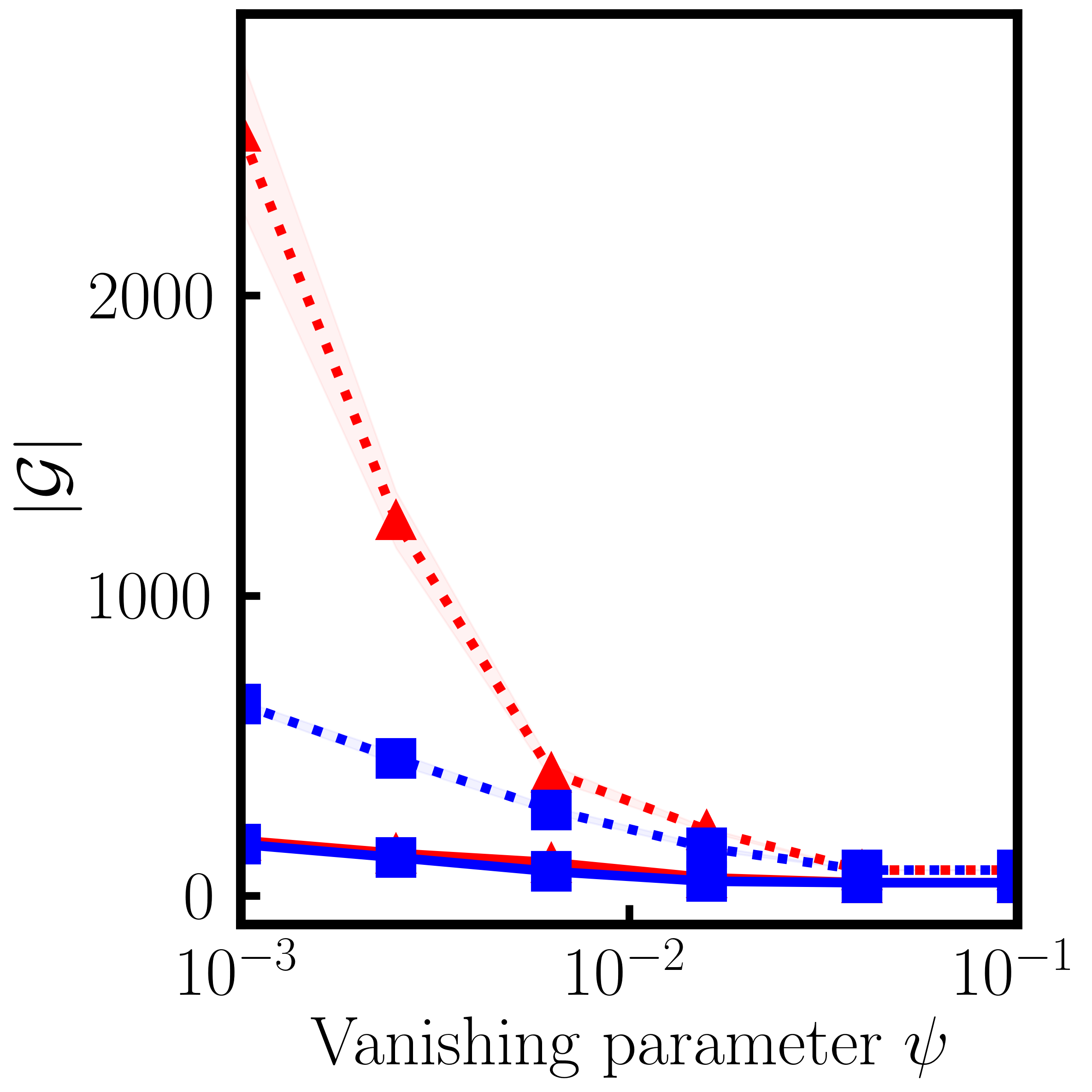
(a) credit

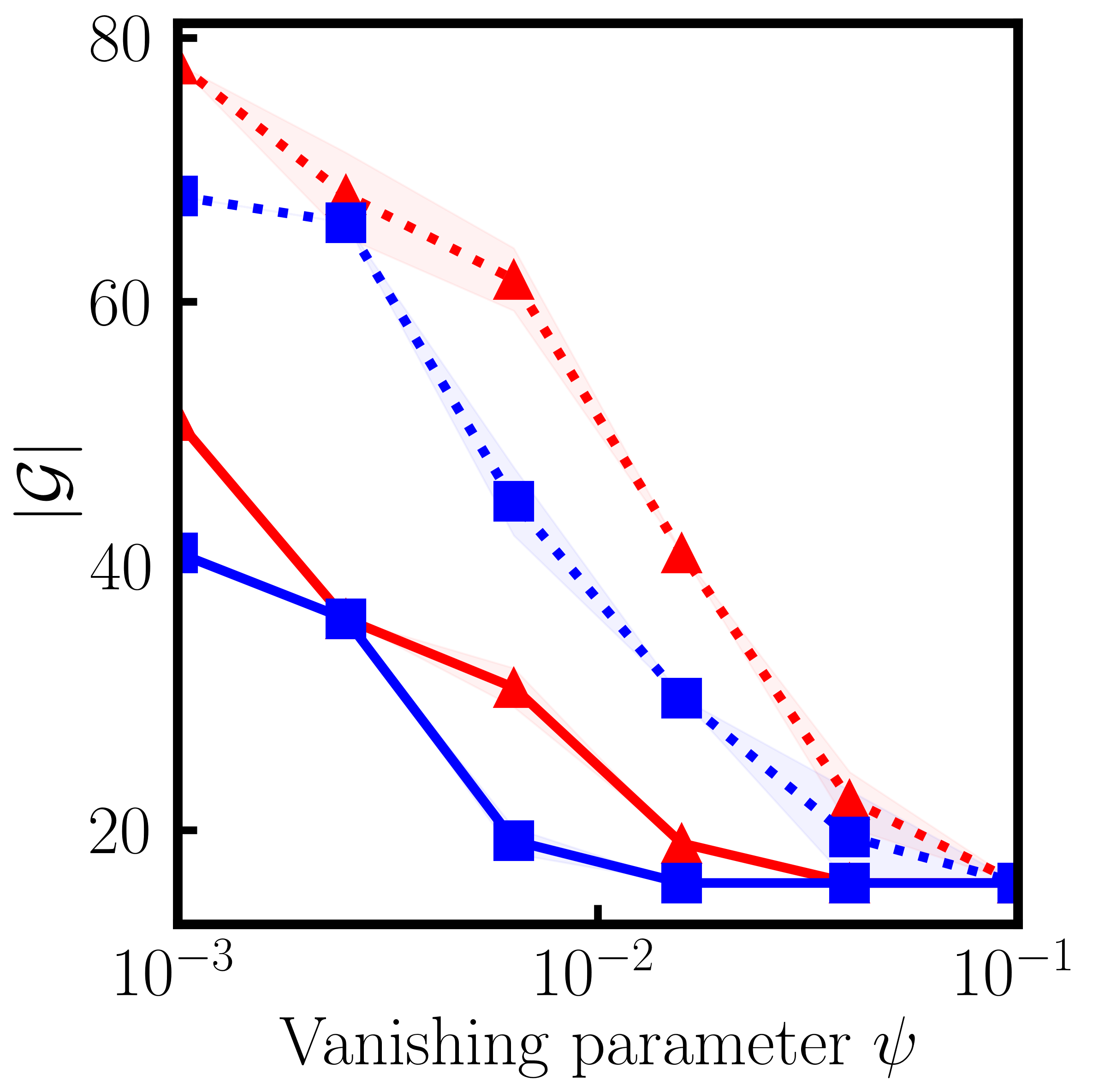
(b) htru

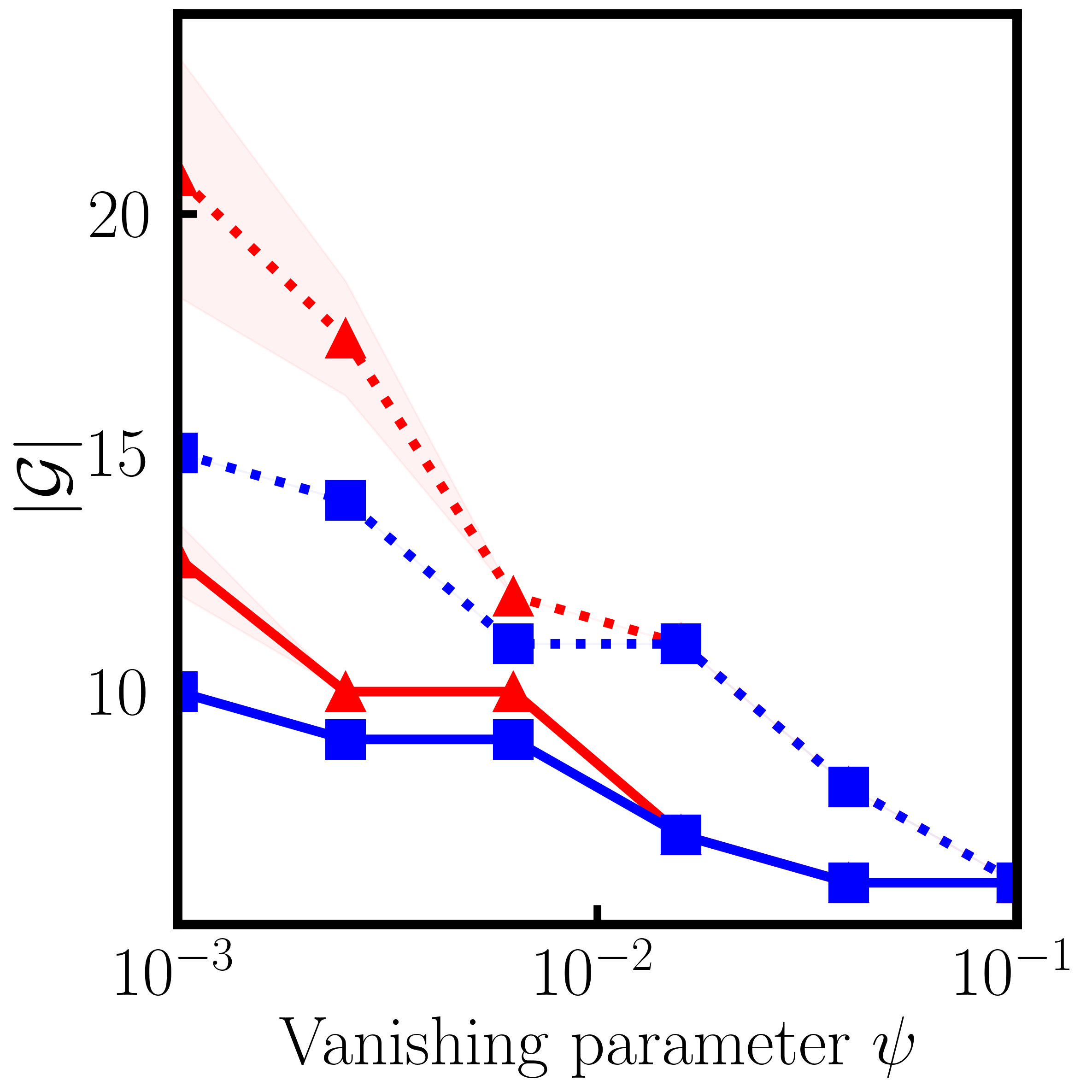
(c) skin

(d) spam

Figure 1: Comparison of the number of generators constructed with PCGAVI and ABM for the border-(GB) and the border-(BB), averaged over ten random runs with shaded standard deviations. Running algorithms with with the border-(BB) often leads to the construction of more generators than with the border-(GB). See Section 9.4 for details on the setup.

9 Numerical Experiments

In this section, we compare the performance of OAVI as a preprocessing technique for a subsequently applied linear kernel SVM to related approaches and determine the influence of the border type on generator-constructing algorithms.

9.1 General Setup

In this section, we present the information relevant to all our numerical experiments.

9.1.1 Implementation

The numerical experiments are implemented in Python and performed on an Nvidia GeForce RTX 3080 GPU with 10GB RAM and an Intel Core i7 11700K 8x CPU at 3.60GHz with 64 GB RAM. Our code is publicly available on GitHub. For all generator-constructing algorithms, we use the definition of $\psi$-approximately vanishing in Definition 2.3.

We implement accelerated gradient descent (AGD) (Nesterov,, 1983) and PCG as ORACLEs in OAVI and refer to the resulting algorithms as PCGAVI, and AGDAVI, respectively. The solvers are run for up to 10,000 iterations. PCG is run up to accuracy $\epsilon=0.001\cdot\psi$. For PCG, we replace (COP) with (CCOP) with $\tau=1000$ and the norm $\|\cdot\|_{1}$. We terminate PCG when less than $0.000001\cdot\psi$ progress is made in absolute difference between function values, when the coefficient vector of a generator is constructed, or if we have a guarantee that no coefficient vector of a generator can be constructed. We terminate AGD when less than $0.000001\cdot\psi$ progress is made in absolute difference between function values for 20 iterations in a row or the coefficient vector of a generator is constructed. Unless noted otherwise, we run OAVI with the border-(GB) as in Definition 4.2.

We implement ABM as presented in Limbeck, (2013) with the modification that instead of applying the SVD to the matrix corresponding to $A={\mathcal{O}}(X)$ in OAVI, we apply the SVD to $A^{\intercal}A$ in case this leads to a faster training time. Unless noted otherwise, we run ABM with the border-(GB) as in Definition 4.2.

We implement VCA as presented in Livni et al., (2013) with the modification that instead of applying the SVD to the matrix corresponding to $A={\mathcal{O}}(X)$ in OAVI, we apply the SVD to $A^{\intercal}A$ in case this leads to a faster training time.

We use a polynomial kernel SVM with one-versus-rest approach from the scikit-learn software package (Pedregosa et al.,, 2011). We run the polynomial kernel SVM with $\ell_{2}$-regularization up to tolerance $10^{-3}$ or for up to 10,000 iterations.

OAVI, ABM, and VCA are used as preprocessing techniques for a subsequently applied linear kernel SVM using the machine learning pipeline discussed in Section 5. We refer to the combined approaches as OAVI^∗, ABM^∗, and VCA^∗, respectively. The linear kernel SVM is implemented using the scikit-learn software package and run with $\ell_{1}$-penalized squared hinge loss up to tolerance $10^{-4}$ or for up to 10,000 iterations.

9.1.2 Hyperparameters

The hyperparameters for PCGAVI^∗, AGDAVI^∗, ABM^∗, and VCA^∗ are the vanishing parameter $\psi\in\{0.1,0.05,0.01,0.005,0.001,0.0005\}$ and the $\ell_{1}$-regularization coefficient of the linear kernel SVM in $\{0.1,1,10\}$. For the polynomial kernel SVM, the hyperparameters are the degree of the kernel in $\{1,2,3,4\}$ and the $\ell_{2}$-regularization coefficient in $\{0.1,1,10\}$.

9.1.3 Data Sets

We provide an overview of the data sets in Table 1. For each data set, we apply min-max feature scaling into the range $[0,1]$ as a preprocessing step.

9.2 Experiment: Performance

Data Set	Full Name	# Samples	# Features
bank	banknote authentication	1,372	4
credit	default of credit cards (Yeh and Lien,, 2009)	30,000	22
htru	HTRU2 (Lyon et al.,, 2016)	17,898	8
seeds	seeds	210	7
skin	skin (Bhatt and Dhall,, 2010)	245,057	3
spam	spambase	4,601	57

Table 1: All data sets are binary classification data sets, except for seeds, which is made up of three classes. The data sets are retrieved from the UCI Machine Learning Repository (Dua and Graff,, 2017) and additional references are provided.

We compare the performance of PCGAVI^∗, AGDAVI^∗, ABM^∗, ABM^∗, and polynomial kernel SVM on various data sets.

9.2.1 Setup

We apply PCGAVI^∗, AGDAVI^∗, ABM^∗, VCA^∗, and polynomial kernel SVM to data sets bank, credit, htru, seeds, skin, and spam. The hyperparameters are tuned on the training data using threefold cross-validation. We retrain the algorithms on the entire training data using the best hyperparameter combination and compare the classification error on the test set, the hyperparameter optimization time, and the test time, that is, the time to evaluate a method on new data. For generator-constructing approaches, we also compare $|{\mathcal{G}}|+|{\mathcal{O}}|$, where $|{\mathcal{G}}|=\sum_{i}|{\mathcal{G}}^{i}|,|{\mathcal{O}}|=\sum_{i}|{\mathcal{O}}^{i}|$, and $({\mathcal{G}}^{i},{\mathcal{O}}^{i})$ is the output of a generator-constructing algorithm applied to samples belonging to class $i$. Moreover, for the generator-constructing approaches, we also compare the sparsity of the feature transformation. The results are averaged over ten random $60\%/40\%$ train/test/partitions.

9.2.2 Results

Algorithms		Data Sets
		bank	credit	htru	seeds	skin	spam
Error Test	PCGAVI∗	$0.51$	$17.96$	$2.11$	$3.69$	$0.26$	$7.16$
	AGDAVI∗	$0.00$	$18.14$	$2.07$	$4.76$	$0.20$	$6.67$
	ABM∗	$0.47$	$18.36$	$2.12$	$5.36$	$0.43$	$7.11$
	VCA∗	$0.16$	$19.85$	$2.11$	$5.00$	$0.24$	$7.15$
	SVM	$0.00$	$18.34$	$2.08$	$4.76$	$2.25$	$7.13$
Time Hyper.	PCGAVI∗	$3.6\times 10^{2}$	$1.1\times 10^{3}$	$3.4\times 10^{2}$	$5.9\times 10^{2}$	$2.3\times 10^{2}$	$2.4\times 10^{3}$
	AGDAVI∗	$2.5\times 10^{1}$	$3.0\times 10^{2}$	$5.9\times 10^{1}$	$4.4\times 10^{1}$	$9.9\times 10^{1}$	$2.1\times 10^{2}$
	ABM∗	$3.7\times 10^{-1}$	$1.5\times 10^{1}$	$7.7\times 10^{0}$	$6.6\times 10^{-1}$	$1.8\times 10^{1}$	$2.2\times 10^{1}$
	VCA∗	$7.6\times 10^{-1}$	$1.7\times 10^{1}$	$4.6\times 10^{0}$	$3.8\times 10^{0}$	$1.3\times 10^{1}$	$3.4\times 10^{1}$
	SVM	$7.0\times 10^{-2}$	$8.9\times 10^{1}$	$4.1\times 10^{0}$	$3.0\times 10^{-2}$	$7.1\times 10^{2}$	$2.2\times 10^{0}$
Time Test	PCGAVI∗	$1.5\times 10^{-3}$	$3.5\times 10^{-3}$	$2.3\times 10^{-3}$	$1.2\times 10^{-3}$	$8.8\times 10^{-3}$	$1.6\times 10^{-3}$
	AGDAVI∗	$1.4\times 10^{-3}$	$6.5\times 10^{-3}$	$1.8\times 10^{-3}$	$1.5\times 10^{-3}$	$8.6\times 10^{-3}$	$1.6\times 10^{-3}$
	ABM∗	$1.2\times 10^{-3}$	$3.\times 10^{-3}$	$1.2\times 10^{-3}$	$1.2\times 10^{-3}$	$7.2\times 10^{-3}$	$1.9\times 10^{-3}$
	VCA∗	$7.1\times 10^{-4}$	$3.1\times 10^{-3}$	$1.3\times 10^{-3}$	$1.4\times 10^{-3}$	$6.8\times 10^{-3}$	$7.6\times 10^{-3}$
	SVM	$2.9\times 10^{-4}$	$1.4\times 10^{0}$	$5.6\times 10^{-2}$	$1.8\times 10^{-4}$	$1.1\times 10^{1}$	$2.\times 10^{-2}$
$|{\mathcal{G}}|+|{\mathcal{O}}|$	PCGAVI∗	$36.80$	$67.30$	$60.00$	$43.50$	$32.30$	$152.10$
	AGDAVI∗	$35.10$	$213.70$	$42.10$	$60.10$	$27.00$	$168.40$
	ABM∗	$28.80$	$51.40$	$18.70$	$37.90$	$19.30$	$259.50$
	VCA∗	$23.80$	$49.80$	$19.00$	$103.10$	$9.00$	$1766.40$
(SPAR)	PCGAVI∗	$0.17$	$0.52$	$0.43$	$0.29$	$0.28$	$0.49$
	AGDAVI∗	$0.00$	$0.00$	$0.00$	$0.00$	$0.00$	$0.01$
	ABM∗	$0.00$	$0.00$	$0.00$	$0.00$	$0.00$	$0.00$
	VCA∗	$0.00$	$0.00$	$0.00$	$0.00$	$0.00$	$0.00$

Table 2: Comparison of test set classification error in percent, hyperparameter optimization time in seconds, and test time in seconds. For the generator-constructing approaches, we also compare the magnitude of $|{\mathcal{G}}|+|{\mathcal{O}}|$ and (SPAR). The results are averaged over ten random $60\%$/$40\%$ train/test partitions and the best results in each category are in bold.

We present the results in Table 2. The classification error on the test set for OAVI^∗ is competitive with other approaches. Indeed, for AGDAVI^∗, the classification error on the test set is either equal to or smaller than the classification error of non-OAVI-based approaches. PCGAVI^∗ tends to perform slightly worse in terms of classification error than AGDAVI^∗ but remains competitive with the other approaches. The hyperparameter optimization time of OAVI^∗ tends to be slower than that of ABM^∗ and VCA^∗. PCGAVI^∗ is always slower than AGDAVI by one order of magnitude. The hyperparameter tuning time of the polynomial kernel SVM tends to be very competitive on smaller data sets. However, on skin, a data set of 245,057 samples, the SVM is slower than all other approaches. The test times of the generator-based approaches tend to be of similar order of magnitudes. For the smaller data sets bank and seeds, the test time of the SVM is faster than that of the generator-based approaches. For larger data sets, however, the test time of the SVM is often multiple orders of magnitude greater than that of the generator-based approaches. For ABM^∗ and VCA^∗, $|{\mathcal{G}}|+|{\mathcal{O}}|$ is often smaller than for OAVI^∗. On spam, the data set with the most features, $|{\mathcal{G}}|+|{\mathcal{O}}|$ is significantly smaller for OAVI^∗ than for ABM^∗ and VCA^∗. Only PCGAVI^∗ constructs sparse feature transformations.

9.3 Experiment: Performance Comparison of Different Border Types

Algorithms		Data Sets
		bank	credit	htru	seeds	skin	spam
Error Test	PCGAVI-(GB)∗	$0.51$	$17.96$	$2.11$	$3.69$	$0.26$	$7.16$
	PCGAVI-(BB)∗	$0.55$	$18.02$	$2.14$	$4.76$	$0.20$	$7.14$
	AGDAVI-(GB)∗	$0.00$	$18.14$	$2.07$	$4.76$	$0.20$	$6.67$
	AGDAVI-(BB)∗	$0.00$	$18.02$	$2.04$	$4.76$	$0.20$	$6.51$
	ABM-(GB)∗	$0.47$	$18.36$	$2.12$	$5.36$	$0.43$	$7.11$
	ABM-(BB)∗	$0.26$	$18.11$	$2.08$	$4.52$	$0.27$	$7.16$
Time Hyper.	PCGAVI-(GB)∗	$3.6\times 10^{2}$	$1.1\times 10^{3}$	$3.4\times 10^{2}$	$5.9\times 10^{2}$	$2.3\times 10^{2}$	$2.4\times 10^{3}$
	PCGAVI-(BB)∗	$4.4\times 10^{2}$	$1.8\times 10^{3}$	$3.7\times 10^{2}$	$7.5\times 10^{2}$	$2.9\times 10^{2}$	$2.5\times 10^{3}$
	AGDAVI-(GB)∗	$2.5\times 10^{1}$	$3.0\times 10^{2}$	$5.9\times 10^{1}$	$4.4\times 10^{1}$	$9.9\times 10^{1}$	$2.1\times 10^{2}$
	AGDAVI-(BB)∗	$3.\times 10^{1}$	$1.0\times 10^{3}$	$1.0\times 10^{2}$	$7.9\times 10^{1}$	$1.4\times 10^{2}$	$3.8\times 10^{2}$
	ABM-(GB)∗	$3.7\times 10^{-1}$	$1.5\times 10^{1}$	$7.7\times 10^{0}$	$6.6\times 10^{-1}$	$1.8\times 10^{1}$	$2.2\times 10^{1}$
	ABM-(BB)∗	$4.4\times 10^{-1}$	$4.1\times 10^{1}$	$8.9\times 10^{0}$	$1.0\times 10^{0}$	$2.3\times 10^{1}$	$4.9\times 10^{1}$
Time Test	PCGAVI-(GB)∗	$1.5\times 10^{-3}$	$3.5\times 10^{-3}$	$2.3\times 10^{-3}$	$1.2\times 10^{-3}$	$8.8\times 10^{-3}$	$1.6\times 10^{-3}$
	PCGAVI-(BB)∗	$1.7\times 10^{-3}$	$3.5\times 10^{-2}$	$2.6\times 10^{-3}$	$1.3\times 10^{-3}$	$1.1\times 10^{-2}$	$3.5\times 10^{-3}$
	AGDAVI-(GB)∗	$1.4\times 10^{-3}$	$6.5\times 10^{-3}$	$1.8\times 10^{-3}$	$1.5\times 10^{-3}$	$8.6\times 10^{-3}$	$1.6\times 10^{-3}$
	AGDAVI-(BB)∗	$1.6\times 10^{-3}$	$2.1\times 10^{-2}$	$2.7\times 10^{-3}$	$1.2\times 10^{-3}$	$8.2\times 10^{-3}$	$3.\times 10^{-3}$
	ABM-(GB)∗	$1.2\times 10^{-3}$	$3.\times 10^{-3}$	$1.2\times 10^{-3}$	$1.2\times 10^{-3}$	$7.2\times 10^{-3}$	$1.9\times 10^{-3}$
	ABM-(BB)∗	$1.3\times 10^{-3}$	$4.7\times 10^{-3}$	$1.7\times 10^{-3}$	$1.4\times 10^{-3}$	$7.9\times 10^{-3}$	$3.9\times 10^{-3}$
$|{\mathcal{G}}|+|{\mathcal{O}}|$	PCGAVI-(GB)∗	$36.80$	$67.30$	$60.00$	$43.50$	$32.30$	$152.10$
	PCGAVI-(BB)∗	$55.10$	$1372.20$	$87.60$	$78.30$	$45.00$	$664.00$
	AGDAVI-(GB)∗	$35.10$	$213.70$	$42.10$	$60.10$	$27.00$	$168.40$
	AGDAVI-(BB)∗	$50.20$	$869.20$	$90.30$	$76.80$	$29.00$	$555.60$
	ABM-(GB)∗	$28.80$	$51.40$	$18.70$	$37.90$	$19.30$	$259.50$
	ABM-(BB)∗	$34.80$	$132.40$	$40.90$	$80.70$	$24.30$	$714.90$
(SPAR)	PCGAVI-(GB)∗	$0.17$	$0.52$	$0.43$	$0.29$	$0.28$	$0.49$
	PCGAVI-(BB)∗	$0.27$	$0.68$	$0.54$	$0.32$	$0.29$	$0.60$
	AGDAVI-(GB)∗	$0.00$	$0.00$	$0.00$	$0.00$	$0.00$	$0.01$
	AGDAVI-(BB)∗	$0.00$	$0.00$	$0.00$	$0.00$	$0.00$	$0.02$
	ABM-(GB)∗	$0.00$	$0.00$	$0.00$	$0.00$	$0.00$	$0.00$
	ABM-(BB)∗	$0.00$	$0.00$	$0.00$	$0.00$	$0.00$	$0.01$

Table 3: Comparison of test set classification error in percent, hyperparameter optimization time in seconds, test time in seconds, magnitude of $|{\mathcal{G}}|+|{\mathcal{O}}|$, and (SPAR). The results are averaged over ten random $60\%$/$40\%$ train/test partitions and the best results in each category are in bold.

We compare the performance of PCGAVI-(GB)^∗, PCGAVI-(BB)^∗, AGDAVI-(GB)^∗, AGDAVI-(BB)^∗, ABM-(GB)^∗, and ABM-(BB)^∗ on various data sets, where the suffixes (BB) and (GB) indicate the use of the border-(BB) and the border-(GB), respectively.

9.3.1 Setup

We repeat the experiment presented in Section 9.2 using the setup from Section 9.2.1 but for algorithms PCGAVI-(GB)^∗, PCGAVI-(BB)^∗, AGDAVI-(GB)^∗, AGDAVI-(BB)^∗, ABM-(GB)^∗, and ABM-(BB)^∗.

9.3.2 Results

The results are presented in Table 3. Note that the results of PCGAVI^∗, AGDAVI^∗, and ABM^∗ in Table 2 correspond to the results of PCGAVI-(GB)^∗, AGDAVI-(GB)^∗, and ABM-(GB)^∗ in Table 3 but are restated for convenience. Running the algorithms with the border-(BB) leads to increased size of the output, $|{\mathcal{G}}|+|{\mathcal{O}}|$, than with the border-(GB). The increased size of the output often leads to longer hyperparameter optimization and test times when algorithms are run with the border-(BB) than with the border-(GB). For PCGAVI^∗, it is not clear whether using the border-(BB) leads to better classification error on the test set than the border-(GB). For AGDAVI^∗ and ABM^∗, the border-(BB) tends to facilitate slightly better classification error on the test set than the border-(GB). Finally, for PCGAVI^∗, the (BB)-variant creates a sparser feature transformation than the (GB)-variant.

9.4 Experiment: Output-Size Comparison for Different Border Types

In this section, we compare the number of constructed generators for PCGAVI-(GB), PCGAVI-(BB), ABM-(GB), and ABM-(BB) for varying vanishing parameters $\psi>0$ on different data sets.

9.4.1 Setup

We apply PCGAVI-(GB), PCGAVI-(BB), ABM-(GB), and ABM-(BB) for different values of $\psi$ to the data sets credit, htru, skin, and spam. We plot the number of constructed generators $|{\mathcal{G}}|=\sum_{i}|{\mathcal{G}}^{i}|$, where ${\mathcal{G}}^{i}$ is the set of generators constructed for class $i$. The results are averaged over ten random runs and standard deviations are shaded.

9.4.2 Results

The results are presented in Figure 1. For all data sets and for both PCGAVI and ABM, we observe that running the algorithms with the border-(GB) leads to the construction of sometimes significantly fewer generators than with the border-(BB).

10 Discussion

We introduced a new algorithm for the construction of generators of the approximate vanishing ideal, OAVI, a framework that captures a theoretically well-motivated variant, PCGAVI. Unlike other vanishing ideal algorithms, PCGAVI constructs generators that are $\tau$-bounded in $\ell_{1}$-norm. As a direct consequence, the algorithm admits three learning guarantees. First, we showed that when a generator $g\in{\mathcal{G}}$ attains a small value on a point ${\mathbf{x}}\in X\subseteq[-1,1]^{n}$ in the training sample, then $g$ also attains small values for samples ${\mathbf{y}}\in[-1,1]^{n}$, whose distance to ${\mathbf{x}}$ is small in $\ell_{\infty}$-norm. Second, under mild assumptions, we showed that generators constructed by PCGAVI are guaranteed to not only vanish approximately on in-sample but also on out-sample data. Third, under mild assumptions, we showed that the combined approach of constructing generators with PCGAVI for a subsequently applied linear kernel SVM admits a margin bound, similar to that of the SVM. Since other generator-constructing algorithms cannot guarantee that the coefficient vectors of constructed generators are $\tau$-bounded in $\ell_{1}$-norm, PCGAVI is the only vanishing ideal algorithm to which these learning guarantees apply. The question remains open whether similar learning guarantees can be derived for related methods. Especially ABM, which guarantees that the coefficient vectors of generators have $\ell_{2}$-norm equal to $1$ is a promising candidate for alternative learning guarantees. An added benefit of PCGAVI is that the coefficient vectors of constructed generators tend to be sparse. The learning guarantees and sparsity of output make PCGAVI a theoretically better supported alternative to ABM, AVI, BB-ABM, and VCA. Numerical experiments indicate that the only drawback of PCGAVI is the increased time required for tuning hyperparameters. Given the strong empirical performance and theoretical guarantees of PCGAVI, we believe the algorithm to be a compelling alternative to related generator-constructing methods.

Acknowledgements

This research was partially funded by the Deutsche Forschungsgemeinschaft (DFG, German Research Foundation) under Germany´s Excellence Strategy – The Berlin Mathematics Research Center MATH⁺ (EXC-2046/1, project ID 390685689, BMS Stipend). We thank Hiroshi Kera for pointing out the connection between OAVI and BB-ABM.

References

• Bach et al., (2012) Bach, F., Lacoste-Julien, S., and Obozinski, G. (2012). On the equivalence between herding and conditional gradient algorithms. In Proceedings of the International Conference on Machine Learning, pages 1355–1362. PMLR.
• Bashiri and Zhang, (2017) Bashiri, M. A. and Zhang, X. (2017). Decomposition-invariant conditional gradient for general polytopes with line search. In Proceedings of Advances in Neural Information Processing Systems, pages 2687–2697.
• Bhatt and Dhall, (2010) Bhatt, R. and Dhall, A. (2010). Skin segmentation dataset. UCI Machine Learning Repository.
• Blondel et al., (2017) Blondel, M., Niculae, V., Otsuka, T., and Ueda, N. (2017). Multi-output polynomial networks and factorization machines. In Proceedings of Advances in Neural Information Processing Systems, pages 3349–3359.
• Bojanowski et al., (2015) Bojanowski, P., Lajugie, R., Grave, E., Bach, F., Laptev, I., Ponce, J., and Schmid, C. (2015). Weakly-supervised alignment of video with text. In Proceedings of the International Conference on Computer Vision, pages 4462–4470. IEEE.
• Braun et al., (2019) Braun, G., Pokutta, S., and Zink, D. (2019). Lazifying conditional gradient algorithms. Journal of Machine Learning Research, 20(71):1–42.
• Combettes and Pokutta, (2020) Combettes, C. and Pokutta, S. (2020). Boosting frank-wolfe by chasing gradients. In Proceedings of the International Conference on Machine Learning, pages 2111–2121. PMLR.
• Courty et al., (2016) Courty, N., Flamary, R., Tuia, D., and Rakotomamonjy, A. (2016). Optimal transport for domain adaptation. IEEE Transactions on Pattern Analysis and Machine Intelligence, 39(9):1853–1865.
• Cox et al., (2013) Cox, D., Little, J., and O’Shea, D. (2013). Ideals, varieties, and algorithms: an introduction to computational algebraic geometry and commutative algebra. Springer Science & Business Media.
• Dua and Graff, (2017) Dua, D. and Graff, C. (2017). UCI machine learning repository.
• Fassino, (2010) Fassino, C. (2010). Almost vanishing polynomials for sets of limited precision points. Journal of Symbolic Computation, 45(1):19–37.
• Frank and Wolfe, (1956) Frank, M. and Wolfe, P. (1956). An algorithm for quadratic programming. Naval Research Logistics Quarterly, 3(1-2):95–110.
• Freund et al., (2017) Freund, R. M., Grigas, P., and Mazumder, R. (2017). An extended Frank-Wolfe method with “in-face” directions, and its application to low-rank matrix completion. SIAM Journal on optimization, 27(1):319–346.
• Garber and Hazan, (2015) Garber, D. and Hazan, E. (2015). Faster rates for the Frank-Wolfe method over strongly-convex sets. In Proceedings of the International Conference on Machine Learning. PMLR.
• Garber and Hazan, (2016) Garber, D. and Hazan, E. (2016). A linearly convergent variant of the conditional gradient algorithm under strong convexity, with applications to online and stochastic optimization. SIAM Journal on Optimization, 26(3):1493–1528.
• Garber and Meshi, (2016) Garber, D. and Meshi, O. (2016). Linear-memory and decomposition-invariant linearly convergent conditional gradient algorithm for structured polytopes. volume 29, pages 1001–1009.
• Giesen et al., (2012) Giesen, J., Jaggi, M., and Laue, S. (2012). Optimizing over the growing spectrahedron. In European Symposium on Algorithms, pages 503–514. Springer.
• Guélat and Marcotte, (1986) Guélat, J. and Marcotte, P. (1986). Some comments on Wolfe’s ‘away step’. Mathematical Programming, 35(1):110–119.
• Harchaoui et al., (2012) Harchaoui, Z., Douze, M., Paulin, M., Dudik, M., and Malick, J. (2012). Large-scale image classification with trace-norm regularization. In Proceedings of the Conference on Computer Vision and Pattern Recognition, pages 3386–3393. IEEE.
• Heldt et al., (2009) Heldt, D., Kreuzer, M., Pokutta, S., and Poulisse, H. (2009). Approximate computation of zero-dimensional polynomial ideals. Journal of Symbolic Computation, 44(11):1566–1591.
• Iraji and Chitsaz, (2017) Iraji, R. and Chitsaz, H. (2017). Principal variety analysis. In Proceedings of the Conference on Robot Learning, pages 97–108.
• Jaggi, (2013) Jaggi, M. (2013). Revisiting Frank-Wolfe: Projection-free sparse convex optimization. In Proceedings of the International Conference on Machine Learning, number CONF, pages 427–435. PMLR.
• Jaggi and Sulovskỳ, (2010) Jaggi, M. and Sulovskỳ, M. (2010). A simple algorithm for nuclear norm regularized problems. In Proceedings of the International Conference on Machine Learning. PMLR.
• Joulin et al., (2014) Joulin, A., Tang, K., and Fei-Fei, L. (2014). Efficient image and video co-localization with frank-wolfe algorithm. In Computer Vision – ECCV 2014, pages 253–268, Cham. Springer International Publishing.
• Kera and Hasegawa, (2019) Kera, H. and Hasegawa, Y. (2019). Spurious vanishing problem in approximate vanishing ideal. IEEE Access, 7:178961–178976.
• Kera and Hasegawa, (2020) Kera, H. and Hasegawa, Y. (2020). Gradient boosts the approximate vanishing ideal. In Proceedings of the Conference on Artificial Intelligence, number 04, pages 4428–4435.
• Kera and Iba, (2016) Kera, H. and Iba, H. (2016). Vanishing ideal genetic programming. In 2016 IEEE Congress on Evolutionary Computation (CEC), pages 5018–5025.
• Kerdreux et al., (2021) Kerdreux, T., Liu, L., Lacoste-Julien, S., and Scieur, D. (2021). Affine invariant analysis of frank-wolfe on strongly convex sets. In Proceedings of the International Conference on Machine Learning, pages 5398–5408. PMLR.
• Kreuzer and Robbiano, (2000) Kreuzer, M. and Robbiano, L. (2000). Computational Commutative Algebra. Springer Berlin Heidelberg.
• Lacoste-Julien and Jaggi, (2013) Lacoste-Julien, S. and Jaggi, M. (2013). An affine invariant linear convergence analysis for Frank-Wolfe algorithms. arXiv preprint arXiv:1312.7864.
• Lacoste-Julien and Jaggi, (2015) Lacoste-Julien, S. and Jaggi, M. (2015). On the global linear convergence of Frank-Wolfe optimization variants. In Proceedings of Advances in Neural Information Processing Systems, pages 496–504.
• Ledoux and Talagrand, (1991) Ledoux, M. and Talagrand, M. (1991). Probability in Banach Spaces: isoperimetry and processes, volume 23. Springer Science & Business Media.
• Levitin and Polyak, (1966) Levitin, E. S. and Polyak, B. T. (1966). Constrained minimization methods. USSR Computational Mathematics and Mathematical Physics, 6(5):1–50.
• Limbeck, (2013) Limbeck, J. (2013). Computation of approximate border bases and applications.
• Livni et al., (2013) Livni, R., Lehavi, D., Schein, S., Nachliely, H., Shalev-Shwartz, S., and Globerson, A. (2013). Vanishing component analysis. In Proceedings of the International Conference on Machine Learning, pages 597–605. PMLR.
• Luise et al., (2019) Luise, G., Salzo, S., Pontil, M., and Ciliberto, C. (2019). Sinkhorn barycenters with free support via Frank-Wolfe algorithm. In Proceedings of Advances in Neural Information Processing Systems, pages 9318–9329.
• Lyon et al., (2016) Lyon, R. J., Stappers, B., Cooper, S., Brooke, J. M., and Knowles, J. D. (2016). Fifty years of pulsar candidate selection: from simple filters to a new principled real-time classification approach. Monthly Notices of the Royal Astronomical Society, 459(1):1104–1123.
• Mohri et al., (2018) Mohri, M., Rostamizadeh, A., and Talwalkar, A. (2018). Foundations of machine learning. MIT press.
• Möller and Buchberger, (1982) Möller, H. M. and Buchberger, B. (1982). The construction of multivariate polynomials with preassigned zeros. In European Computer Algebra Conference, pages 24–31. Springer.
• Nesterov, (1983) Nesterov, Y. (1983). A method for unconstrained convex minimization problem with the rate of convergence $O(1/k^{2})$. In Doklady an USSR, volume 269, pages 543–547.
• Paty and Cuturi, (2019) Paty, F.-P. and Cuturi, M. (2019). Subspace robust wasserstein distances. In Proceedings of the International Conference on Machine Learning, pages 5072–5081. PMLR.
• Pedregosa et al., (2011) Pedregosa, F., Varoquaux, G., Gramfort, A., Michel, V., Thirion, B., Grisel, O., Blondel, M., Prettenhofer, P., Weiss, R., Dubourg, V., et al. (2011). Scikit-learn: Machine learning in python. Journal of Machine Learning Research, 12:2825–2830.
• Peyre et al., (2017) Peyre, J., Sivic, J., Laptev, I., and Schmid, C. (2017). Weakly-supervised learning of visual relations. In Proceedings of the International Conference on Computer Vision, pages 5179–5188. IEEE.
• Ping et al., (2016) Ping, W., Liu, Q., and Ihler, A. T. (2016). Learning infinite rbms with Frank-Wolfe. In Proceedings of Advances in Neural Information Processing Systems, pages 3063–3071.
• Suykens and Vandewalle, (1999) Suykens, J. A. and Vandewalle, J. (1999). Least squares support vector machine classifiers. Neural Processing Letters, 9(3):293–300.
• Wang and Ohtsuki, (2018) Wang, L. and Ohtsuki, T. (2018). Nonlinear blind source separation unifying vanishing component analysis and temporal structure. IEEE Access, 6:42837–42850.
• Yeh and Lien, (2009) Yeh, I.-C. and Lien, C.-H. (2009). The comparisons of data mining techniques for the predictive accuracy of probability of default of credit card clients. Expert Systems with Applications, 36(2):2473–2480.
• Zhang, (2018) Zhang, X. (2018). Improvement on the vanishing component analysis by grouping strategy. EURASIP Journal on Wireless Communications and Networking, 2018(1):111.
• Zhao and Song, (2014) Zhao, Y.-G. and Song, Z. (2014). Hand posture recognition using approximate vanishing ideal generators. In Proceedings of the International Conference on Image Processing, pages 1525–1529. IEEE.