Neighbor2Seq: Deep Learning on Massive Graphs by Transforming Neighbors to Sequences

Abstract

Modern graph neural networks (GNNs) use a message passing scheme and have achieved great success in many fields. However, this recursive design inherently leads to excessive computation and memory requirements, making it not applicable to massive real-world graphs. In this work, we propose the Neighbor2Seq to transform the hierarchical neighborhood of each node into a sequence. This novel transformation enables the subsequent mini-batch training for general deep learning operations, such as convolution and attention, that are designed for grid-like data and are shown to be powerful in various domains. Therefore, our Neighbor2Seq naturally endows GNNs with the efficiency and advantages of deep learning operations on grid-like data by precomputing the Neighbor2Seq transformations. We evaluate our method on a massive graph, with more than $111$ million nodes and $1.6$ billion edges, as well as several medium-scale graphs. Results show that our proposed method is scalable to massive graphs and achieves superior performance across massive and medium-scale graphs. Our code is available at https://github.com/divelab/Neighbor2Seq.

1 Introduction

Graph neural networks (GNNs) have shown effectiveness in many fields with rich relational structures, such as citation networks [25, 36], social networks [17], drug discovery [15, 33, 39], physical systems [4], and point clouds [38]. Most current GNNs follow a message passing scheme [15, 5], in which the representation of each node is recursively updated by aggregating the representations of its neighbors. Various GNNs [28, 25, 36, 41] mainly differ in the forms of aggregation functions.

Real-world applications usually generate massive graphs, such as social networks. However, message passing methods have difficulties in handling such large graphs as the recursive message passing mechanism leads to prohibitive computation and memory requirements. To date, sampling methods [17, 43, 10, 9, 22, 46, 45, 14, 11, 45] and precomputing methods [40, 32, 6] have been proposed to scale GNNs on large graphs, as reviewed and analyzed in Section 2.2. While the sampling methods can speed up training, they might result in redundancy, still incur high computational complexity, lead to loss of performance, or introduce bias. Generally, precomputing methods can scale to larger graphs as compared to sampling methods as recursive message passing is still required in sampling methods.

In this work, we propose the Neighbor2Seq that transforms the hierarchical neighborhood of each node to a sequence in a precomputing step. After the Neighbor2Seq transformation, each node and its associated neighborhood tree are converted to an ordered sequence. Therefore, each node can be viewed as an independent sample and is no longer constrained by the topological structure. This novel transformation from graphs to grid-like data enables the use of mini-batch training for subsequent models. As a result, our models can be used on extremely large graphs, as long as the Neighbor2Seq step can be precomputed.

As a radical departure from existing precomputing methods, including SGC [40] and SIGN [32], we consider the hierarchical neighborhood of each node as an ordered sequence. This order information corresponding to hops between nodes is preserved in our Neighbor2Seq and captured explicitly in subsequent order sensitive operations, such as convolutions. This order information is vital for improving the prediction, as confirmed by our experiments and ablation studies in Section 5. As a result of our Neighbor2Seq transformation, generic and powerful deep learning operations for grid-like data, such as convolution and attention, can be applied in subsequent models to learn from the resulting sequences. Experimental results indicate that our proposed method can be used on a massive graph, where most current methods cannot be applied. Furthermore, our method achieves superior performance as compared with previous sampling and precomputing methods.

2 Analysis of Current Graph Neural Network Methods

We start by defining necessary notations. A graph is formally defined as $\mathcal{G}=(V,E)$, where $V$ is the set of nodes and $E\subseteq V\times V$ is the set of edges. We use $n=|V|$ and $m=|E|$ to denote the numbers of nodes and edges, respectively. The nodes are indexed from $1$ to $n$. We consider a node feature matrix $\boldsymbol{X}\in\mathbb{R}^{n\times d}$, where each row $\boldsymbol{x}_{i}\in\mathbb{R}^{d}$ is the $d$-dimensional feature vector associated with node $i$. The topology information of the graph is encoded in the adjacency matrix $\boldsymbol{A}\in\mathbb{R}^{n\times n}$, where $\boldsymbol{A}_{(i,j)}=1$ if an edge exists between node $i$ and node $j$, and $\boldsymbol{A}_{(i,j)}=0$ otherwise. Although we describe our approach on undirected graphs for simplicity, it can be naturally applied on directed graphs.

2.1 Graph Neural Networks via Message Passing.

There are two primary deep learning methods on graphs [7]; those are, spectral methods [8] and spatial methods. In this work, we focus on the analysis of the current mainstream spatial methods. Generally, most existing spatial methods, such as ChebNet [12], GCN [25], GG-NN [28], GAT [36], and GIN [41], can be understood from the message passing perspective [15, 5]. Specifically, we iteratively update node representations by aggregating representations from its immediate neighbors. These message passing methods have been shown to be effective in many fields. However, they have inherent difficulties when applied on large graphs due to their excessive computation and memory requirements, as described in Section 2.2.

2.2 Graph Neural Networks on Large Graphs.

The above message passing methods are often trained in full batch. This requires the whole graph, i.e., all the node representations and edge connections, to be in memory to allow recursive message passing on the whole graph. Usually, the number of neighbors grows very rapidly with the increase of receptive field [1]. Hence, these methods cannot be applied directly on large-scale graphs due to the prohibitive computation and memory. To enable deep learning on large graphs, two families of methods have been proposed; those are methods based on sampling and precomputing.

To circumvent the recursive expansion of neighbors across layers, sampling methods apply GNNs on a sampled subset of nodes with mini-batch training. Sampling methods can be further divided into three categories. First, node-wise sampling methods perform message passing for each node in its sampled neighborhood. This strategy is first proposed in GraphSAGE [17], where neighbors are randomly sampled. This is extended by PinSAGE [43], which selects neighbors based on random walks. VR-GCN [10] further proposes to use variance reduction techniques to obtain a convergence guarantee. Although these node-wise sampling methods can reduce computation, the remaining computation is still very expensive and some redundancy might have been introduced, as described in [22]. Second, layer-wise sampling methods sample a fixed number of nodes for each layer of GNNs. In particular, FastGCN [9] samples a fixed number of nodes for each layer independently based on the degree of each node. AS-GCN [22] and LADIES [46] introduce between-layer dependencies during sampling, thus alleviating the loss of information. Layer-wise sampling methods can avoid the redundancy introduced by node-wise sampling methods. However, the expensive sampling algorithms that aim to ensure performance may themselves incur high computational cost, as pointed out in [45]. Third, graph-wise sampling methods build mini-batches on sampled subgraphs. Specifically, LGCN [14] proposes to leverage mini-batch training on subgraphs selected by Breadth-First-Search algorithms. ClusterGCN [11] conducts mini-batch training on sampled subgraphs that are obtained by a graph clustering algorithm. GraphSAINT [45] proposes to derive subgraphs by importance-sampling and introduces normalization techniques to eliminate biases. These graph-wise sampling methods usually have high efficiency. The main limitation is that the nodes in a sampled subgraph are usually clustered together. This implies that two distant nodes in the original graph usually cannot be feeded into the GNNs in the same mini-batch during training, potentially leading to bias in the trained models.

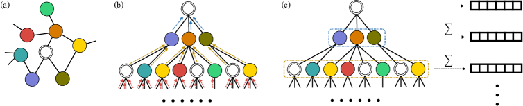
Figure 1: (a) An illustration of the original graph. The current node is denoted as two concentric circles. (b) Message passing in the neighborhood tree. (c) Our proposed Neighbor2Seq.

The second family of methods for enabling GNNs training on large graphs are based on precomputing. Specifically, SGC [40] removes the non-linearity between GCN layers, resulting in a simplification as $\boldsymbol{Y}=\textrm{softmax}(\boldsymbol{\hat{A}}^{L}\boldsymbol{X}\boldsymbol{W})$. In this formulation, $\boldsymbol{\hat{A}}=\boldsymbol{\tilde{D}}^{-\frac{1}{2}}\boldsymbol{\tilde{A}}\boldsymbol{\tilde{D}}^{-\frac{1}{2}}$ is the symmetrically normalized adjacency matrix, $\boldsymbol{\tilde{A}}=\boldsymbol{A}+\boldsymbol{I}$ is the adjacency matrix with self-loops, $\boldsymbol{\tilde{D}}$ is the corresponding diagonal node degree matrix with $\boldsymbol{\tilde{D}}_{(i,i)}=\sum_{j}\boldsymbol{\tilde{A}}_{(i,j)}$, $L$ is the size of receptive field (i.e., the number of considered neighboring hops), which is the same as an $L$-layer GCN, $\boldsymbol{Y}$ is the output of the softmax classifier. Since there is no learnable parameters in $\boldsymbol{\hat{A}}^{L}\boldsymbol{X}$, this term can be precomputed as a feature pre-processing step. Similarly, SIGN [32] applies an inception-like model to the precomputed features $\boldsymbol{\hat{A}}^{\ell}\boldsymbol{X}$ for $\ell\in\{1,\cdots,L\}$, where $L$ is the predefined size of receptive field. Instead of precomputing the smoothing features as in SGC and SIGN, PPRGo [6] extends the idea of PPNP [26] by approximately precomputing the personalized PageRank [29] matrix, thereby enabling model training on large graphs using mini-batches. Generally, the precomputing methods can scale to larger graphs because the sampling methods still need to perform the recursive message passing during training. Differing from these precomputing methods, we consider the hierarchical neighborhood of each node as an ordered sequence, thus retaining the useful information about hops between nodes and enabling subsequent powerful and efficient operations.

3 The Proposed Neighbor2Seq Method and Analysis

In this section, we firstly describe our proposed method, known as Neighbor2Seq, which transforms the hierarchical neighborhood of each node into an ordered sequence, thus enabling the subsequent use of general deep learning operations. Then, we analyze the scalability of our method (Section 3.5).

3.1 Overview.

As described in Section 2.1, existing message passing methods recursively update each node’s representation by aggregating information from its immediate neighbors. Hence, what these methods aim at capturing for each node is essentially its corresponding hierarchical neighborhood, i.e., the neighborhood tree rooted at the current node, as illustrated in Figure 1 (b). In this work, we attempt to go beyond the message passing scheme to overcome the limitations mentioned in Section 2.2. We propose to capture the information of this hierarchical neighborhood by transforming it into an ordered sequence, instead of recursively squashing it into a fixed-length vector. Our proposed method is composed of three steps. First, we transform the neighborhood to a sequence for each node. Second, we apply a normalization technique to the derived sequence features. Third, we use general deep learning operations, i.e., convolution and attention, to learn from these sequence features and then make predictions for nodes. In the following, we describe these three steps in detail.

3.2 Neighbor2Seq: Transforming Neighborhoods to Sequences.

The basic idea of the proposed Neighbor2Seq is to transform the hierarchical neighborhood of each node to an ordered sequence by integrating the features of nodes in each layer of the neighborhood tree. Following the notations defined in Section 2, we let $\boldsymbol{z}^{i}_{0},\boldsymbol{z}^{i}_{1},\cdots,\boldsymbol{z}^{i}_{L}$ denote the resulting sequence for node $i$, where $L$ is the height of the neighborhood tree rooted at node $i$, i.e., the number of hops we consider. $\boldsymbol{z}^{i}_{\ell}\in\mathbb{R}^{d}$ denotes the $\ell$-th feature of the sequence. The length of the resulting sequence for each node is $L+1$. Formally, for each node $i$, our Neighbor2Seq can be expressed as

(3.1) $$\boldsymbol{z}^{i}_{\ell}=\sum_{j=1}^{n}w(i,j,\ell)\boldsymbol{x}_{j},\quad\forall\ell\in\{0,1,2,\cdots,L\},$$

where $w(i,j,\ell)$ denotes the number of walks with length $\ell$ between node $i$ and $j$. $n$ is the number of nodes in the graph. We define $w(i,j,0)$ as $1$ for $j=i$ and $0$ otherwise. Hence, $\boldsymbol{z}^{i}_{0}$ is the original node feature $\boldsymbol{x}_{i}$. Intuitively, $\boldsymbol{z}^{i}_{\ell}$ is obtained by computing a weighted sum of features of all nodes with walks of length $\ell$ to $i$, and the numbers of qualified walks are used as the corresponding weights. Our Neighbor2Seq is illustrated in Figure 1 (c). Note that the derived sequence has meaningful order information, indicating the hops between nodes. After we obtain ordered sequences from the original hierarchical neighborhoods, we can use generic deep learning operations to learn from these sequences, as detailed below.

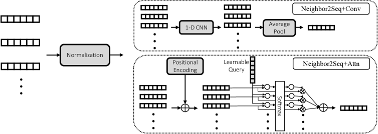
Figure 2: An illustration of our proposed models: Neighbor2Seq+Conv and Neighbor2Seq+Attn.

3.3 Normalization.

Since the number of nodes in the hierarchical neighborhood grows exponentially as the hop number increases, different layers in the neighborhood tree have drastically different numbers of nodes. Hence, feature vectors of a sequence computed by Eq. (3.1) have very different scales. In order to make the subsequent learning easier, we propose a layer to normalize the sequence features. We use a normalization technique similar to layer normalization [2]. In particular, each feature of a sequence is normalized based on the mean and the standard deviation of its own feature values. Formally, our normalization process for each node $i$ can be written as

(3.2) $$\boldsymbol{y}^{i}_{\ell} =\boldsymbol{W_{\ell}}\boldsymbol{z}^{i}_{\ell}, \quad\forall\ell\in\{0,1,2,\cdots,L\},$$

$$\boldsymbol{o}^{i}_{\ell} =\frac{\boldsymbol{y}^{i}_{\ell}-\mu^{i}_{\ell}}{\sigma^{i}_{\ell}}\odot\boldsymbol{\gamma}_{\ell}+\boldsymbol{\beta}_{\ell}, \quad\forall\ell\in\{0,1,2,\cdots,L\},$$

where $\mu^{i}_{\ell}$ and $\sigma^{i}_{\ell}$ denote the corresponding mean and standard deviation of the representation $\boldsymbol{y}^{i}_{\ell}$. Formally,

(3.3) $$\mu^{i}_{\ell}=\frac{1}{d^{\prime}}\sum_{c=1}^{d^{\prime}}\boldsymbol{y}^{i}_{\ell}[c],\quad\sigma^{i}_{\ell}=\sqrt{\frac{1}{d^{\prime}}\sum_{c=1}^{d^{\prime}}(\boldsymbol{y}^{i}_{\ell}[c]-\mu^{i}_{\ell})^{2}}.$$

We first apply a learnable linear transformation $\boldsymbol{W_{\ell}}\in\mathbb{R}^{d^{\prime}\times d}$ to produce a low-dimensional representation $\boldsymbol{y}^{i}_{\ell}\in\mathbb{R}^{d^{\prime}}$ for the $\ell$-th feature of the sequence, since the original feature dimension $d$ is usually large. $\boldsymbol{\gamma}_{\ell}\in\mathbb{R}^{d^{\prime}}$ and $\boldsymbol{\beta}_{\ell}\in\mathbb{R}^{d^{\prime}}$ denote the learnable affine transformation parameters. $\odot$ denotes the element-wise multiplication. Note that the learnable parameters in this normalization layer is associated with $\ell$, implying that each feature of the sequence is normalized separately. Using this normalization layer, we obtain the normalized feature vector $\boldsymbol{o}^{i}_{\ell}\in\mathbb{R}^{d^{\prime}}$ for every $\ell\in\{0,1,2,\cdots,L\}$.

3.4 Neighbor2Seq+Conv and Neighbor2Seq+Attn.

After obtaining an ordered sequence for each node, we can view each node in the graph as a sequence of feature vectors. We can use general deep learning techniques to learn from these sequences. In this work, we propose two models, namely Neighbor2Seq+Conv and Neighbor2Seq+Attn, in which convolution and attention are applied to the sequences of each node accordingly.

As illustrated in Figure 2, Neighbor2Seq+Conv applies a 1-D convolutional neural network to the sequence features and then use an average pooling to yield a representation for the sequence. Formally, for each node $i$,

(3.4) $$\left(\boldsymbol{\hat{o}}^{i}_{0},\boldsymbol{\hat{o}}^{i}_{1},\cdots,\boldsymbol{\hat{o}}^{i}_{L}\right) =\textrm{CNN}\left(\boldsymbol{o}^{i}_{0},\boldsymbol{o}^{i}_{1},\cdots,\boldsymbol{o}^{i}_{L}\right),$$

$$\boldsymbol{r}^{i} =\frac{1}{L+1}\sum_{\ell=0}^{L}\boldsymbol{\hat{o}}^{i}_{\ell},$$

where $\textrm{CNN}(\cdot)$ denotes a 1-D convolutional neural network. $\boldsymbol{r}^{i}$ denotes the obtained representation of node $i$ that is used as the input to a linear classifier to make prediction for this node. Specifically, we implement $\textrm{CNN}(\cdot)$ as a 2-layer convolutional neural network composed of two 1-D convolutions. The activation function between layers is ReLU [27].

Incorporating attention is another natural idea to learn from sequences. As shown in Figure 2, Neighbor2Seq+Attn uses an attention mechanism [3] to integrate sequential feature vectors in order to derive an informative representation for each node. Unlike convolutional neural networks, the vanilla attention mechanism cannot make use of the order of the sequence. Hence, we add positional encodings [35] to the features such that the position information of different features in the sequence can be incorporated. Formally, for each node $i$, we add positional encoding for each feature in the sequence as

(3.5) $$\boldsymbol{p}^{i}_{\ell}[m] =\left\{\begin{aligned} &\sin\left(\frac{\ell}{10000^{\frac{2n}{d^{\prime}}}}\right)\quad m=2n&\\ &\cos\left(\frac{\ell}{10000^{\frac{2n}{d^{\prime}}}}\right)\quad m=2n+1&\end{aligned},\right.$$

$$\boldsymbol{k}^{i}_{\ell} =\boldsymbol{o}^{i}_{\ell}+\boldsymbol{p}^{i}_{\ell}.$$

The positional encoding for $\ell$-th feature of node $i$ is denoted as $\boldsymbol{p}^{i}_{\ell}\in\mathbb{R}^{d^{\prime}}$. $m\in\{1,2,\cdots,d^{\prime}\}$ is the dimensional index. Intuitively, a position-dependent vector is added to each feature such that the order information can be captured. Then we use the attention mechanism with learnable query [42] to combine these sequential feature vectors to obtain the final representations $\boldsymbol{r}^{i}$ for each node $i$. Formally,

(3.6) $$\boldsymbol{r}^{i}=\sum_{\ell=0}^{L}\alpha^{i}_{\ell}\boldsymbol{k}^{i}_{\ell},\quad\alpha^{i}_{\ell}=\frac{\exp({\boldsymbol{k}^{i}_{\ell}}^{T}\boldsymbol{q})}{\sum_{\ell=0}^{L}\exp({\boldsymbol{k}^{i}_{\ell}}^{T}\boldsymbol{q})}.$$

$\boldsymbol{q}\in\mathbb{R}^{d^{\prime}}$ is the learnable query vector that is trained along with other model parameters. The derived representation $\boldsymbol{r}^{i}$ will be taken as the input to a linear classifier to make prediction for node $i$.

3.5 Analysis of Scalability.

(i) Precomputing Neighbor2Seq. A well-known fact is that the value of $w(i,j,\ell)$ in Eq. (3.1) can be obtained by computing the power of the original adjacency matrix $\boldsymbol{A}$. Following GCN, we add self-loops to make each node connect to itself. Concretely, $w(i,j,\ell)=\boldsymbol{\tilde{A}}^{\ell}_{(i,j)}$, where $\boldsymbol{\tilde{A}}=\boldsymbol{A}+\boldsymbol{I}$. Hence, the Neighbor2Seq can be implemented by computing the matrix multiplications $\boldsymbol{\tilde{A}}^{\ell}\boldsymbol{X}$ for $\forall\ell\in\{0,1,2,\cdots,L\}$. Note that we do not need to normalize the adjacency matrix in our Neighbor2Seq, differing from popular GNNs, such as GCN, and existing precomputing methods, such as SGC and SIGN. Since there is no learnable parameters in the Neighbor2Seq step, these matrix multiplications can be precomputed sequentially for large graphs on CPU platforms with large memory. This can be easily precomputed because the matrix $\boldsymbol{\tilde{A}}$ is usually sparse. For extremely large graphs, this precomputation can even be performed on distributed systems.

(ii) Enabling mini-batch training. After we obtain the precomputed sequence features, each node in the graph corresponds to a sequence of feature vectors. Therefore, each node can be viewed as an independent sample. That is, we are no longer restricted by the original graph connectivity. Then, we can randomly sample from all the training nodes to conduct mini-batch training. This is more flexible and unbiased than sampling methods as reviewed in Section 2.2. Our mini-batches can be randomly extracted over all nodes, opening the possibility that any pair of nodes can be sampled in the same mini-batch. In contrast, mini-batches in sampling methods are usually restricted by the fixed sampling strategies. This advantage opens the door for subsequent model training on extremely large graphs, as long as the corresponding Neighbor2Seq step can be precomputed.

Table 1: Comparison of computational complexity for precomputing and forward pass (per epoch).

Method	Precomputing	Forward Pass
GCN	-	$\mathcal{O}(Ldm+Ld^{2}n)$
GraphSAGE	$\mathcal{O}(s^{L}n)$	$\mathcal{O}(s^{L}d^{2}n)$
ClusterGCN	$\mathcal{O}(m)$	$\mathcal{O}(Ldm+Ld^{2}n)$
GraphSAINT	$\mathcal{O}(sn)$	$\mathcal{O}(Ldm+Ld^{2}n)$
SGC	$\mathcal{O}(Ldm)$	$\mathcal{O}(d^{2}n)$
SIGN	$\mathcal{O}(Ldm)$	$\mathcal{O}(Ld^{2}n)$
Neighbor2Seq+Conv	$\mathcal{O}(Ldm)$	$\mathcal{O}((Ld^{2}+Lkd^{2})n)$
Neighbor2Seq+Attn	$\mathcal{O}(Ldm)$	$\mathcal{O}((Ld^{2}+Ld)n)$

Table 2: Statistics of datasets. “m” denotes multi-label classification.

Dataset	Scale	Task	#Nodes	#Edges	Avg. Deg.	#Features	#Classes	Train/Val/Test
ogbn-papers100M	Massive	Transductive	$111,059,956$	$1,615,685,872$	$29$	$128$	$172$	$0.78/0.08/0.14$
ogbn-products	Medium	Transductive	$2,449,029$	$61,859,140$	$51$	$100$	$47$	$0.08/0.02/0.90$
Reddit	Medium	Inductive	$232,965$	$11,606,919$	$50$	$602$	$41$	$0.66/0.10/0.24$
Yelp	Medium	Inductive	$716,857$	$6,997,410$	$10$	$300$	$100$(m)	$0.75/0.10/0.15$
Flickr	Medium	Inductive	$89,250$	$899,756$	$10$	$500$	$7$	$0.50/0.25/0.25$

Table 3: Results on ogbn-papers100M in terms of classification accuracy (in percent). The reported accuracy is averaged over $10$ random runs. The best performance on test set is highlighted in bold and the second performance is shown with an underline.

Method	Training	Validation	Test
MLP	$54.84\scriptstyle{{{\color[rgb]{0.3,0.3,0.3}\pm 0.43}}}$	$49.60\scriptstyle{{{\color[rgb]{0.3,0.3,0.3}\pm 0.29}}}$	$47.24\scriptstyle{{{\color[rgb]{0.3,0.3,0.3}\pm 0.31}}}$
Node2vec	-	$58.07\scriptstyle{{{\color[rgb]{0.3,0.3,0.3}\pm 0.28}}}$	$55.60\scriptstyle{{{\color[rgb]{0.3,0.3,0.3}\pm 0.23}}}$
SGC	$67.54\scriptstyle{{{\color[rgb]{0.3,0.3,0.3}\pm 0.43}}}$	$66.48\scriptstyle{{{\color[rgb]{0.3,0.3,0.3}\pm 0.20}}}$	$63.29\scriptstyle{{{\color[rgb]{0.3,0.3,0.3}\pm 0.19}}}$
Neighbor2Seq+Conv	$70.94\scriptstyle{{{\color[rgb]{0.3,0.3,0.3}\pm 1.40}}}$	$68.19\scriptstyle{{{\color[rgb]{0.3,0.3,0.3}\pm 0.32}}}$	$\textbf{65.62}\scriptstyle{{{\color[rgb]{0.3,0.3,0.3}\pm 0.32}}}$
Neighbor2Seq+Attn	$70.75\scriptstyle{{{\color[rgb]{0.3,0.3,0.3}\pm 0.68}}}$	$67.60\scriptstyle{{{\color[rgb]{0.3,0.3,0.3}\pm 0.31}}}$	$\underline{65.04}\scriptstyle{{{\color[rgb]{0.3,0.3,0.3}\pm 0.24}}}$

(iii) Computational complexity comparison. We compare our methods with several existing sampling and precomputing methods in terms of computational complexity. We let $L$ denote the number of hops we consider. For simplicity, we assume the feature dimension $d$ is fixed for all layers. For sampling methods, $s$ is the number of sampled neighbors for each node. The computation of Neighbor2Seq+Conv mainly lies in the linear transformation (i.e., $\mathcal{O}(Ld^{2}n)$) in the normalization step and the 1-D convolutional neural networks (i.e., $\mathcal{O}(Lkd^{2}n)$, where $k$ is the kernel size). Hence, the computational complexity for the forward pass of Neighbor2Seq+Conv is $\mathcal{O}((Ld^{2}+Lkd^{2})n)$. Neighbor2Seq+Attn has a computational complexity of $\mathcal{O}((Ld^{2}+Ld)n)$ because the attention mechanism using learnable query is more efficient than 1-D convolutional neural networks. As shown in Table 1, the forward pass complexities of precomputing methods, including our Neighbor2Seq+Conv and Neighbor2Seq+Attn, are all linear with respect to the number of nodes $n$ and do not depend on the number of edges $m$. Hence, the training processes of our models are computationally efficient. Compared with existing precomputing methods, our models, especially Neighbor2Seq+Conv, are slightly more time consuming due to the introduced convolution or attention operations. However, our models have the same order of time complexity as existing precomputing methods, i.e., being linear with respect to the number of nodes $n$. Also, in practice, the generic deep learning operations, such as convolution and attention, are well accelerated and parallelized in modern platforms. Hence, our method achieves better balance between performance and efficiency. We compare actual running time to demonstrate this in Section 5.4.

4 Discussions

The main difference between graph and grid-like data lies in the notion and properties of locality. Specifically, the numbers of neighbors differ for different nodes, and there is no order information among the neighbors of a node in graphs. These are the main obstacles preventing the use of generic deep learning operations on graphs. Our Neighbor2Seq is an attempt to bridge the gap between graph and grid-like data. Base on our Neighbor2Seq, many effective strategies for grid-like data can be naturally transferred to graph data. These include self-supervised learning and pre-training on graphs [20, 37, 34, 18, 44, 21, 31, 24].

We notice an existing work AWE [23] which also embed the information in graph as a sequence. In order to avoid confusion, we make a clarification about the fundamental and significant differences between AWE and our Neighbor2Seq. First, AWE produces a sequence embedding for the entire graph, while our Neighbor2Seq yields a sequence embedding for each node in the graph. Second, each element in the obtained sequence in AWE is the probability of an anonymous walk embedding. In our Neighbor2Seq, each feature vector in the obtained sequence for one node is computed by summing up the features of all nodes in the corresponding layer of the neighborhood tree. This point distinguishes these two methods fundamentally.

More discussions about our method are included in the Supplementary Material.

5 Experimental Studies

5.1 Experimental Setup.

(i) Datasets. We evaluate our proposed models by performing node classification tasks on $1$ massive-scale graph (ogbn-papers100M [19]) and $4$ medium-scale graphs (ogbn-products [19], Reddit [17], Yelp [45], and Flickr [45]). These tasks cover inductive and transductive settings. The statistics of these datasets are summarized in Table 2. The detailed description of these datasets are provided in the Supplementary Material.

(ii) Implementation. We implemented our methods using Pytorch [30] and Pytorch Geometric [13]. For our proposed methods, we conduct the precomputation on a CPU, after which we train our models on a GeForce RTX 2080 Ti GPU. We perform a grid search for the following hyperparameters: number of hops $L$, batch size, learning rate, hidden dimension $d^{\prime}$, dropout rate, weight decay, and convolutional kernel size $k$.

5.2 Results on Massive-Scale Graphs.

Since ogbn-papers100M is a massive graph with more than $111$ million nodes and $1.6$ billion edges, most existing methods have difficulty handling such a graph. We consider three baselines that have available results evaluated by OGB [19]: Multilayer Perceptron (MLP), Node2Vec [16], and SGC [40]. Note that the existing sampling methods cannot be applied to this massive graph. The results under transductive setting is reported in Table 3. Following OGB, we report accuracies for all models on training, validation, and test sets. Our models outperform the baselines consistently in terms of training, validation, and test. In particular, our Neighbor2Seq+Conv performs better than SGC by an obvious margin of $2.33\%$ in terms of test accuracy. This demonstrates the expressive power and the generalization ability of our method on massive graphs.

5.3 Results on Medium-Scale Graphs.

We also evaluate our models on medium-scale graphs, thus enabling comparison with more existing strong baselines. We conduct transductive learning on ogbn-products, a medium-scale graph from OGB. We also conduct inductive learning on Reddit, Yelp, and Flickr, which are frequently used for inductive learning by the community. The following various baselines are considered: MLP, Node2Vec [16], GCN [25], SGC [40], GraphSAGE [17], FastGCN [9], VR-GCN [10], AS-GCN [22], ClusterGCN [11], GraphSAINT [45], and SIGN [32].

Table 4: Results on ogbn-products in terms of classification accuracy (in percent). The reported accuracy is averaged over $10$ random runs. Obtaining the results of GCN requires a GPU with 33GB of memory. The best performance on test set is highlighted in bold and the second performance is shown with an underline.

Method	Training	Validation	Test
MLP	$84.03\scriptstyle{{{\color[rgb]{0.3,0.3,0.3}\pm 0.93}}}$	$75.54\scriptstyle{{{\color[rgb]{0.3,0.3,0.3}\pm 0.14}}}$	$61.06\scriptstyle{{{\color[rgb]{0.3,0.3,0.3}\pm 0.08}}}$
Node2vec	$93.39\scriptstyle{{{\color[rgb]{0.3,0.3,0.3}\pm 0.10}}}$	$90.32\scriptstyle{{{\color[rgb]{0.3,0.3,0.3}\pm 0.06}}}$	$72.49\scriptstyle{{{\color[rgb]{0.3,0.3,0.3}\pm 0.10}}}$
GCN	$93.56\scriptstyle{{{\color[rgb]{0.3,0.3,0.3}\pm 0.09}}}$	$92.00\scriptstyle{{{\color[rgb]{0.3,0.3,0.3}\pm 0.03}}}$	$75.64\scriptstyle{{{\color[rgb]{0.3,0.3,0.3}\pm 0.21}}}$
GraphSAGE	$92.96\scriptstyle{{{\color[rgb]{0.3,0.3,0.3}\pm 0.07}}}$	$91.70\scriptstyle{{{\color[rgb]{0.3,0.3,0.3}\pm 0.09}}}$	$78.70\scriptstyle{{{\color[rgb]{0.3,0.3,0.3}\pm 0.36}}}$
ClusterGCN	$93.75\scriptstyle{{{\color[rgb]{0.3,0.3,0.3}\pm 0.13}}}$	$92.12\scriptstyle{{{\color[rgb]{0.3,0.3,0.3}\pm 0.09}}}$	$78.97\scriptstyle{{{\color[rgb]{0.3,0.3,0.3}\pm 0.33}}}$
GraphSAINT	$92.71\scriptstyle{{{\color[rgb]{0.3,0.3,0.3}\pm 0.14}}}$	$91.62\scriptstyle{{{\color[rgb]{0.3,0.3,0.3}\pm 0.08}}}$	$79.08\scriptstyle{{{\color[rgb]{0.3,0.3,0.3}\pm 0.24}}}$
SGC	$92.60\scriptstyle{{{\color[rgb]{0.3,0.3,0.3}\pm 0.10}}}$	$91.19\scriptstyle{{{\color[rgb]{0.3,0.3,0.3}\pm 0.06}}}$	$72.46\scriptstyle{{{\color[rgb]{0.3,0.3,0.3}\pm 0.27}}}$
SIGN	$96.92\scriptstyle{{{\color[rgb]{0.3,0.3,0.3}\pm 0.46}}}$	$93.10\scriptstyle{{{\color[rgb]{0.3,0.3,0.3}\pm 0.08}}}$	$77.60\scriptstyle{{{\color[rgb]{0.3,0.3,0.3}\pm 0.13}}}$
Neighbor2Seq+Conv	$95.32\scriptstyle{{{\color[rgb]{0.3,0.3,0.3}\pm 0.10}}}$	$92.92\scriptstyle{{{\color[rgb]{0.3,0.3,0.3}\pm 0.05}}}$	$\textbf{79.67}\scriptstyle{{{\color[rgb]{0.3,0.3,0.3}\pm 0.16}}}$
Neighbor2Seq+Attn	$92.82\scriptstyle{{{\color[rgb]{0.3,0.3,0.3}\pm 0.14}}}$	$92.20\scriptstyle{{{\color[rgb]{0.3,0.3,0.3}\pm 0.02}}}$	$\underline{79.35}\scriptstyle{{{\color[rgb]{0.3,0.3,0.3}\pm 0.17}}}$

The ogbn-products dataset is challenging because the splitting is not random. As described in Section 5.1, the splitting procedure is more realistic and matches the real-world application where manual labeling is prioritized to important nodes and models are subsequently used to make prediction on less important nodes. Also, we only have $10\%$ nodes for training and validation in ogbn-products. Hence, ogbn-products is an ideal benchmark dataset to evaluate the capability of out-of-distribution prediction. As shown in Table 4, our Neighbor2Seq+Conv and Neighbor2Seq+Attn outperfom baselines on test set (i.e., $90\%$ nodes), which further demonstrates the generalization ability of our method on limited training data.

Table 5: Results for inductive learning on three datasets in terms of F1-micro score. The reported score is averaged over $10$ random runs. The results of baselines are partially obtained from [45, 32]. For each dataset, the best performance on test set is highlighted in bold and the second performance is shown with an underline.

Method	Reddit	Flickr	Yelp
GCN	$0.933\scriptstyle{{{\color[rgb]{0.3,0.3,0.3}\pm 0.000}}}$	$0.492\scriptstyle{{{\color[rgb]{0.3,0.3,0.3}\pm 0.003}}}$	$0.378\scriptstyle{{{\color[rgb]{0.3,0.3,0.3}\pm 0.001}}}$
FastGCN	$0.924\scriptstyle{{{\color[rgb]{0.3,0.3,0.3}\pm 0.001}}}$	$0.504\scriptstyle{{{\color[rgb]{0.3,0.3,0.3}\pm 0.001}}}$	$0.265\scriptstyle{{{\color[rgb]{0.3,0.3,0.3}\pm 0.053}}}$
VR-GCN	$0.964\scriptstyle{{{\color[rgb]{0.3,0.3,0.3}\pm 0.001}}}$	$0.482\scriptstyle{{{\color[rgb]{0.3,0.3,0.3}\pm 0.003}}}$	$0.640\scriptstyle{{{\color[rgb]{0.3,0.3,0.3}\pm 0.002}}}$
AS-GCN	$0.958\scriptstyle{{{\color[rgb]{0.3,0.3,0.3}\pm 0.001}}}$	$0.504\scriptstyle{{{\color[rgb]{0.3,0.3,0.3}\pm 0.002}}}$	-
GraphSAGE	$0.953\scriptstyle{{{\color[rgb]{0.3,0.3,0.3}\pm 0.001}}}$	$0.501\scriptstyle{{{\color[rgb]{0.3,0.3,0.3}\pm 0.013}}}$	$0.634\scriptstyle{{{\color[rgb]{0.3,0.3,0.3}\pm 0.006}}}$
ClusterGCN	$0.954\scriptstyle{{{\color[rgb]{0.3,0.3,0.3}\pm 0.001}}}$	$0.481\scriptstyle{{{\color[rgb]{0.3,0.3,0.3}\pm 0.005}}}$	$0.609\scriptstyle{{{\color[rgb]{0.3,0.3,0.3}\pm 0.005}}}$
GraphSAINT	$0.966\scriptstyle{{{\color[rgb]{0.3,0.3,0.3}\pm 0.001}}}$	$0.511\scriptstyle{{{\color[rgb]{0.3,0.3,0.3}\pm 0.001}}}$	$\textbf{0.653}\scriptstyle{{{\color[rgb]{0.3,0.3,0.3}\pm 0.003}}}$
SGC	$0.949\scriptstyle{{{\color[rgb]{0.3,0.3,0.3}\pm 0.000}}}$	$0.502\scriptstyle{{{\color[rgb]{0.3,0.3,0.3}\pm 0.001}}}$	$0.358\scriptstyle{{{\color[rgb]{0.3,0.3,0.3}\pm 0.006}}}$
SIGN	$\textbf{0.968}\scriptstyle{{{\color[rgb]{0.3,0.3,0.3}\pm 0.000}}}$	$0.514\scriptstyle{{{\color[rgb]{0.3,0.3,0.3}\pm 0.001}}}$	$0.631\scriptstyle{{{\color[rgb]{0.3,0.3,0.3}\pm 0.003}}}$
Neighbor2Seq+Conv	$\underline{0.967}\scriptstyle{{{\color[rgb]{0.3,0.3,0.3}\pm 0.000}}}$	$\textbf{0.527}\scriptstyle{{{\color[rgb]{0.3,0.3,0.3}\pm 0.003}}}$	$\underline{0.647}\scriptstyle{{{\color[rgb]{0.3,0.3,0.3}\pm 0.003}}}$
Neighbor2Seq+Attn	$\underline{0.967}\scriptstyle{{{\color[rgb]{0.3,0.3,0.3}\pm 0.000}}}$	$\underline{0.523}\scriptstyle{{{\color[rgb]{0.3,0.3,0.3}\pm 0.002}}}$	$\underline{0.647}\scriptstyle{{{\color[rgb]{0.3,0.3,0.3}\pm 0.001}}}$

The results on inductive tasks are summarized in Table 5. On Reddit, our models perform better than all sampling methods and achieve the competitive result as SIGN. On Flickr, our models obtain significantly better results. Specifically, our Neighbor2Seq+Conv outperforms the previous state-of-the-art models by an obvious margin. Although our models perform not as good as GraphSAINT on Yelp, we outperform other sampling methods and the precomputing model SIGN consistently on this dataset. To the best of our knowledge, there does not exist a method that can perform best overwhelmingly on all these datasets for inductive tasks currently. Therefore, we believe the experimental results can clearly demonstrate the effectiveness of our methods for inductive learning.

Table 6: Computational efficiency in terms of preprocessing and training (per epoch) (in seconds) on ogbn-products. The reported time is averaged over $10$ runs. The test performance is included for reference.

Method	Preproc. ($\downarrow$)	Train ($\downarrow$)	Test Acc. ($\uparrow$)
ClusterGCN	$44.15\scriptstyle{{{\color[rgb]{0.3,0.3,0.3}\pm 0.77}}}$	$11.87\scriptstyle{{{\color[rgb]{0.3,0.3,0.3}\pm 0.84}}}$	$78.97\scriptstyle{{{\color[rgb]{0.3,0.3,0.3}\pm 0.33}}}$
GraphSAINT	$80.78\scriptstyle{{{\color[rgb]{0.3,0.3,0.3}\pm 3.5}}}$	$4.29\scriptstyle{{{\color[rgb]{0.3,0.3,0.3}\pm 0.48}}}$	$79.08\scriptstyle{{{\color[rgb]{0.3,0.3,0.3}\pm 0.24}}}$
SGC	$153.36\scriptstyle{{{\color[rgb]{0.3,0.3,0.3}\pm 3.6}}}$	$0.15\scriptstyle{{{\color[rgb]{0.3,0.3,0.3}\pm 0.01}}}$	$72.46\scriptstyle{{{\color[rgb]{0.3,0.3,0.3}\pm 0.27}}}$
SIGN	$151.47\scriptstyle{{{\color[rgb]{0.3,0.3,0.3}\pm 3.5}}}$	$1.22\scriptstyle{{{\color[rgb]{0.3,0.3,0.3}\pm 0.02}}}$	$77.60\scriptstyle{{{\color[rgb]{0.3,0.3,0.3}\pm 0.13}}}$
Neighbor2Seq+Conv	$153.42\scriptstyle{{{\color[rgb]{0.3,0.3,0.3}\pm 3.2}}}$	$4.09\scriptstyle{{{\color[rgb]{0.3,0.3,0.3}\pm 0.12}}}$	$79.67\scriptstyle{{{\color[rgb]{0.3,0.3,0.3}\pm 0.16}}}$
Neighbor2Seq+Attn	$153.42\scriptstyle{{{\color[rgb]{0.3,0.3,0.3}\pm 3.2}}}$	$2.67\scriptstyle{{{\color[rgb]{0.3,0.3,0.3}\pm 0.08}}}$	$79.35\scriptstyle{{{\color[rgb]{0.3,0.3,0.3}\pm 0.17}}}$

Table 7: Comparison of models with and without capturing order information. Neighbor2Seq+Attn w/o PE denotes the Neighbor2Seq+Attn without adding positional encoding. For each dataset, the best performance on test set is highlighted in bold and the second performance is shown with an underline.

Model	Order information	ogbn-papers100M	ogbn-products	Reddit	Flickr	Yelp
Neighbor2Seq+Conv	✓	$\textbf{65.62}\scriptstyle{{{\color[rgb]{0.3,0.3,0.3}\pm 0.32}}}$	$\textbf{79.67}\scriptstyle{{{\color[rgb]{0.3,0.3,0.3}\pm 0.16}}}$	$\textbf{0.967}\scriptstyle{{{\color[rgb]{0.3,0.3,0.3}\pm 0.000}}}$	$\textbf{0.527}\scriptstyle{{{\color[rgb]{0.3,0.3,0.3}\pm 0.003}}}$	$\textbf{0.647}\scriptstyle{{{\color[rgb]{0.3,0.3,0.3}\pm 0.003}}}$
Neighbor2Seq+Attn	✓	$\underline{65.04}\scriptstyle{{{\color[rgb]{0.3,0.3,0.3}\pm 0.24}}}$	$\underline{79.35}\scriptstyle{{{\color[rgb]{0.3,0.3,0.3}\pm 0.17}}}$	$\textbf{0.967}\scriptstyle{{{\color[rgb]{0.3,0.3,0.3}\pm 0.000}}}$	$\underline{0.523}\scriptstyle{{{\color[rgb]{0.3,0.3,0.3}\pm 0.002}}}$	$\textbf{0.647}\scriptstyle{{{\color[rgb]{0.3,0.3,0.3}\pm 0.001}}}$
Neighbor2Seq+Attn w/o PE	✗	$65.03\scriptstyle{{{\color[rgb]{0.3,0.3,0.3}\pm 0.42}}}$	$78.54\scriptstyle{{{\color[rgb]{0.3,0.3,0.3}\pm 0.25}}}$	$0.965\scriptstyle{{{\color[rgb]{0.3,0.3,0.3}\pm 0.000}}}$	$0.521\scriptstyle{{{\color[rgb]{0.3,0.3,0.3}\pm 0.003}}}$	$0.646\scriptstyle{{{\color[rgb]{0.3,0.3,0.3}\pm 0.001}}}$

5.4 Comparisons of Computional Efficiency.

In order to verify our analysis of time complexity in Section 3.5, we conduct an empirical comparison with existing methods in terms of real running time during preprocessing and training. We consider the following representative sampling methods and precomputing methods: ClusterGCN [11], GraphSAINT [45], SGC [40], and SIGN [32]. The comparison is performed on ogbn-products and the similar trend can be observed on other datasets. As demonstrated in Table 6, our approaches, like existing precomputing methods, are more computationally efficient than sampling methods in terms of training. Although the precomputing methods cost more time on preprocessing, this precomputing only need to be conducted by one time. Compared with existing precomputing methods, our methods obtain better performance with introducing affordable computation, achieving a better balance between performance and efficiency.

5.5 Ablation Study on Order Information

Intuitively, the order information in the sequence obtained by Neighbor2Seq indicates the hops between nodes. Hence, we conduct an ablation study to verify the significance of this order information. We remove the positional encoding in Neighbor2Seq+Attn, leading to a model without the ability to capture the order information. The comparison is demonstrated in Table 7. Note that Neighbor2Seq+Attn and Neighbor2Seq+Attn w/o PE have the same number of parameters. Hence, Comparing the results of these two models, we can conclude that the order information is usually necessary and the degree of importance depends on the corresponding dataset. Both Neighbor2Seq+Conv and Neighbor2Seq+Attn can capture the order information. We observe that Neighbor2Seq+Conv performs better. The possible reason could be that Neighbor2Seq+Conv has more learnable parameters than Neighbor2Se+Attn, which only has a learnable query.

6 Conclusions

In this work, we propose Neighbor2Seq, for transforming the heirarchical neighborhoods to ordered sequences. Neighbor2Seq enables the subsequent use of powerful general deep learning operations, leading to the proposed Neighbor2Seq+Conv and Neighbor2Seq+Attn. Our models can be deployed on massive graphs and trained efficiently. The extensive expriments demonstrate the scalability and the promising performance of our method.

References

- [1] U. Alon and E. Yahav. On the bottleneck of graph neural networks and its practical implications. arXiv preprint arXiv:2006.05205, 2020.
- [2] J. L. Ba, J. R. Kiros, and G. E. Hinton. Layer normalization. arXiv preprint arXiv:1607.06450, 2016.
- [3] D. Bahdanau, K. Cho, and Y. Bengio. Neural machine translation by jointly learning to align and translate. In International Conference on Learning Representations, 2015.
- [4] P. Battaglia, R. Pascanu, M. Lai, D. J. Rezende, et al. Interaction networks for learning about objects, relations and physics. In Advances in neural information processing systems, pages 4502–4510, 2016.
- [5] P. W. Battaglia, J. B. Hamrick, V. Bapst, A. Sanchez-Gonzalez, V. Zambaldi, M. Malinowski, A. Tacchetti, D. Raposo, A. Santoro, R. Faulkner, et al. Relational inductive biases, deep learning, and graph networks. arXiv preprint arXiv:1806.01261, 2018.
- [6] A. Bojchevski, J. Klicpera, B. Perozzi, A. Kapoor, M. Blais, B. Rózemberczki, M. Lukasik, and S. Günnemann. Scaling graph neural networks with approximate pagerank. In Proceedings of the 26th ACM SIGKDD International Conference on Knowledge Discovery & Data Mining, pages 2464–2473, 2020.
- [7] M. M. Bronstein, J. Bruna, Y. LeCun, A. Szlam, and P. Vandergheynst. Geometric deep learning: going beyond euclidean data. IEEE Signal Processing Magazine, 34(4):18–42, 2017.
- [8] J. Bruna, W. Zaremba, A. Szlam, and Y. LeCun. Spectral networks and locally connected networks on graphs. In International Conference on Learning Representations, 2014.
- [9] J. Chen, T. Ma, and C. Xiao. Fastgcn: Fast learning with graph convolutional networks via importance sampling. In International Conference on Learning Representations, 2018.
- [10] J. Chen, J. Zhu, and L. Song. Stochastic training of graph convolutional networks with variance reduction. In International Conference on Machine Learning, pages 942–950, 2018.
- [11] W.-L. Chiang, X. Liu, S. Si, Y. Li, S. Bengio, and C.-J. Hsieh. Cluster-gcn: An efficient algorithm for training deep and large graph convolutional networks. In Proceedings of the 25th ACM SIGKDD International Conference on Knowledge Discovery & Data Mining, pages 257–266, 2019.
- [12] M. Defferrard, X. Bresson, and P. Vandergheynst. Convolutional neural networks on graphs with fast localized spectral filtering. In Advances in Neural Information Processing Systems, pages 3844–3852, 2016.
- [13] M. Fey and J. E. Lenssen. Fast graph representation learning with PyTorch Geometric. In ICLR Workshop on Representation Learning on Graphs and Manifolds, 2019.
- [14] H. Gao, Z. Wang, and S. Ji. Large-scale learnable graph convolutional networks. In Proceedings of the 24th ACM SIGKDD International Conference on Knowledge Discovery & Data Mining, pages 1416–1424, 2018.
- [15] J. Gilmer, S. S. Schoenholz, P. F. Riley, O. Vinyals, and G. E. Dahl. Neural message passing for quantum chemistry. In Proceedings of the 34th international conference on machine learning, pages 1263–1272, 2017.
- [16] A. Grover and J. Leskovec. node2vec: Scalable feature learning for networks. In Proceedings of the 22nd ACM SIGKDD international conference on Knowledge discovery and data mining, pages 855–864, 2016.
- [17] W. Hamilton, Z. Ying, and J. Leskovec. Inductive representation learning on large graphs. In Advances in Neural Information Processing Systems, pages 1024–1034, 2017.
- [18] K. Hassani and A. H. Khasahmadi. Contrastive multi-view representation learning on graphs. In International Conference on Machine Learning, 2020.
- [19] W. Hu, M. Fey, M. Zitnik, Y. Dong, H. Ren, B. Liu, M. Catasta, and J. Leskovec. Open graph benchmark: Datasets for machine learning on graphs. Advances in Neural Information Processing Systems, 2020.
- [20] W. Hu, B. Liu, J. Gomes, M. Zitnik, P. Liang, V. Pande, and J. Leskovec. Strategies for pre-training graph neural networks. In International Conference on Learning Representations, 2019.
- [21] Z. Hu, Y. Dong, K. Wang, K.-W. Chang, and Y. Sun. Gpt-gnn: Generative pre-training of graph neural networks. In Proceedings of the 26th ACM SIGKDD International Conference on Knowledge Discovery & Data Mining, pages 1857–1867, 2020.
- [22] W. Huang, T. Zhang, Y. Rong, and J. Huang. Adaptive sampling towards fast graph representation learning. In Advances in neural information processing systems, pages 4558–4567, 2018.
- [23] S. Ivanov and E. Burnaev. Anonymous walk embeddings. In Proceedings of the 35th International Conference on Machine Learning, volume 80, pages 2191–2200. PMLR, 2018.
- [24] W. Jin, T. Derr, H. Liu, Y. Wang, S. Wang, Z. Liu, and J. Tang. Self-supervised learning on graphs: Deep insights and new direction. arXiv preprint arXiv:2006.10141, 2020.
- [25] T. N. Kipf and M. Welling. Semi-supervised classification with graph convolutional networks. In International Conference on Learning Representations, 2017.
- [26] J. Klicpera, A. Bojchevski, and S. Günnemann. Predict then propagate: Graph neural networks meet personalized pagerank. In International Conference on Learning Representations, 2019.
- [27] A. Krizhevsky, I. Sutskever, and G. E. Hinton. Imagenet classification with deep convolutional neural networks. Advances in neural information processing systems, 25:1097–1105, 2012.
- [28] Y. Li, D. Tarlow, M. Brockschmidt, and R. Zemel. Gated graph sequence neural networks. In International Conference on Learning Representations, 2016.
- [29] L. Page, S. Brin, R. Motwani, and T. Winograd. The pagerank citation ranking: Bringing order to the web. Technical report, Stanford InfoLab, 1999.
- [30] A. Paszke, S. Gross, S. Chintala, G. Chanan, E. Yang, Z. DeVito, Z. Lin, A. Desmaison, L. Antiga, and A. Lerer. Automatic differentiation in pytorch. 2017.
- [31] J. Qiu, Q. Chen, Y. Dong, J. Zhang, H. Yang, M. Ding, K. Wang, and J. Tang. Gcc: Graph contrastive coding for graph neural network pre-training. In Proceedings of the 26th ACM SIGKDD International Conference on Knowledge Discovery & Data Mining, pages 1150–1160, 2020.
- [32] E. Rossi, F. Frasca, B. Chamberlain, D. Eynard, M. Bronstein, and F. Monti. Sign: Scalable inception graph neural networks. arXiv preprint arXiv:2004.11198, 2020.
- [33] J. M. Stokes, K. Yang, K. Swanson, W. Jin, A. Cubillos-Ruiz, N. M. Donghia, C. R. MacNair, S. French, L. A. Carfrae, Z. Bloom-Ackerman, et al. A deep learning approach to antibiotic discovery. Cell, 180(4):688–702, 2020.
- [34] F.-Y. Sun, J. Hoffman, V. Verma, and J. Tang. Infograph: Unsupervised and semi-supervised graph-level representation learning via mutual information maximization. In International Conference on Learning Representations, 2019.
- [35] A. Vaswani, N. Shazeer, N. Parmar, J. Uszkoreit, L. Jones, A. N. Gomez, Ł. Kaiser, and I. Polosukhin. Attention is all you need. In Advances in Neural Information Processing Systems, pages 5998–6008, 2017.
- [36] P. Veličković, G. Cucurull, A. Casanova, A. Romero, P. Lio, and Y. Bengio. Graph attention networks. In International Conference on Learning Representation, 2018.
- [37] P. Velickovic, W. Fedus, W. L. Hamilton, P. Liò, Y. Bengio, and R. D. Hjelm. Deep graph infomax. In International Conference on Learning Representations, 2019.
- [38] Y. Wang, Y. Sun, Z. Liu, S. E. Sarma, M. M. Bronstein, and J. M. Solomon. Dynamic graph cnn for learning on point clouds. Acm Transactions On Graphics (tog), 38(5):1–12, 2019.
- [39] Z. Wang, M. Liu, Y. Luo, Z. Xu, Y. Xie, L. Wang, L. Cai, and S. Ji. Advanced graph and sequence neural networks for molecular property prediction and drug discovery. arXiv preprint arXiv:2012.01981, 2020.
- [40] F. Wu, A. Souza, T. Zhang, C. Fifty, T. Yu, and K. Weinberger. Simplifying graph convolutional networks. In International Conference on Machine Learning, pages 6861–6871, 2019.
- [41] K. Xu, W. Hu, J. Leskovec, and S. Jegelka. How powerful are graph neural networks? In International Conference on Learning Representations, 2019.
- [42] Z. Yang, D. Yang, C. Dyer, X. He, A. Smola, and E. Hovy. Hierarchical attention networks for document classification. In Proceedings of the 2016 Conference of the North American chapter of the Association for Computational Linguistics: Human Language Technologies, pages 1480–1489, 2016.
- [43] R. Ying, R. He, K. Chen, P. Eksombatchai, W. L. Hamilton, and J. Leskovec. Graph convolutional neural networks for web-scale recommender systems. In Proceedings of the 24th ACM SIGKDD International Conference on Knowledge Discovery & Data Mining, pages 974–983, 2018.
- [44] Y. You, T. Chen, Z. Wang, and Y. Shen. When does self-supervision help graph convolutional networks? In International Conference on Machine Learning, 2020.
- [45] H. Zeng, H. Zhou, A. Srivastava, R. Kannan, and V. Prasanna. Graphsaint: Graph sampling based inductive learning method. In International Conference on Learning Representations, 2020.
- [46] D. Zou, Z. Hu, Y. Wang, S. Jiang, Y. Sun, and Q. Gu. Layer-dependent importance sampling for training deep and large graph convolutional networks. In Advances in Neural Information Processing Systems, pages 11249–11259, 2019.