Motion-Plane-Adaptive Inter Prediction
in 360-Degree Video Coding

Abstract

Inter prediction is one of the key technologies enabling the high compression efficiency of modern video coding standards. 360-degree video needs to be mapped to the 2D image plane prior to coding in order to allow compression using existing video coding standards. The distortions that inevitably occur when mapping spherical data onto the 2D image plane, however, impair the performance of classical inter prediction techniques.
In this paper, we propose a motion-plane-adaptive inter prediction technique (MPA) for 360-degree video that takes the spherical characteristics of 360-degree video into account. Based on the known projection format of the video, MPA allows to perform inter prediction on different motion planes in 3D space instead of having to work on the - in theory arbitrarily mapped - 2D image representation directly. We furthermore derive a motion-plane-adaptive motion vector prediction technique (MPA-MVP) that allows to translate motion information between different motion planes and motion models. Our proposed integration of MPA together with MPA-MVP into the state-of-the-art H.266/VVC video coding standard shows significant Bjøntegaard Delta rate savings of 1.72% with a peak of 3.97% based on PSNR and 1.56% with a peak of 3.40% based on WS-PSNR compared to the VTM-14.2 baseline on average.

I Introduction

The all-around field of view of 360-degree video combined with stereo capture technologies capable of creating a sense of virtual depth allows to create virtual reality (VR) experiences providing an unprecedented feeling of immersion. With the increasing availability of affordable VR headsets, 360-degree video has the potential to be the next major evolutionary step in video technology.

((a)) ERP-projected 360-degree image

((b)) sphere mapping (front)

((c)) sphere mapping (back)

Figure 1: (a) A 360-degree image mapped to the 2D image plane using an equirectangular projection (ERP). (b), (c) The 360-degree image mapped to the unit sphere in 3D space visualizing (b) the front view and (c) the back view.

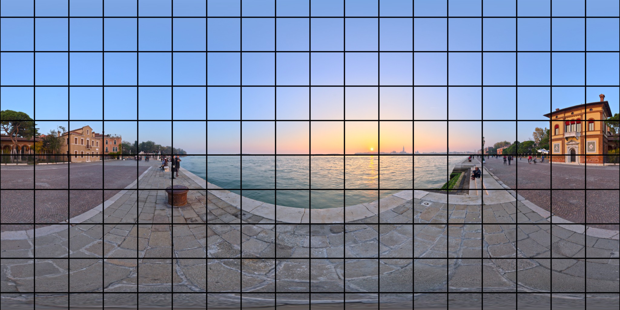
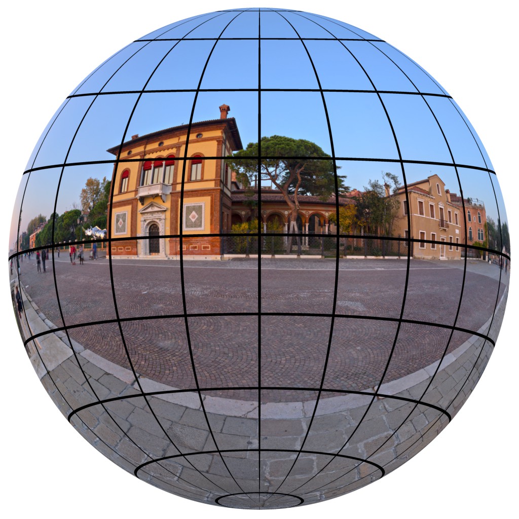
The delivery of immersive 360-degree VR experiences can be divided into three main areas: capture, storage & distribution, and display. Our research addresses the second area, more specifically, the development and design of improved coding techniques for 360-degree video compression. Typically, a 2D representation of the 360-degree video is required to allow compression using existing video coding techniques such as the H.264/AVC [1], the H.265/HEVC [2] or the H.266/VVC [3, 4] video coding standards. Fig. 1(a) shows an example of a 360-degree image mapped to the 2D image plane through an equirectangular projection (ERP). While this is one of the most common 360-degree projection formats, there exist a plethora of other formats including various variations of cubemap projections, segmented and rotated sphere projections, or octa- and icosahedron projections to name only a few [5].

Compared to coding conventional perspective video, the compression performance of modern video codecs is notably reduced for non-perspective projection formats [6, 4]. One reason for this are the distortions that inevitably occur due to the mapping of the spherical 360-degree video to the 2D image plane. Fig. 1(b) and (c) show the spherical domain representation of the ERP-projected 360-degree image in Fig. 1(a). While the black lines of constant azimuthal (vertical) and polar (horizontal) angles form a block structure in the ERP-projected image, this is not the case in the spherical domain. It is clearly visible that the different blocks become increasingly distorted with a higher distance to the equator.

This makes the investigation of inter prediction techniques in the context of 360-degree video coding especially important. In classical translational inter prediction, each block in a regarded frame is predicted from a shifted block in a known reference frame whereby the block retains its size and shape. However, as can be seen in Fig. 1, the further to the poles an object lies, the higher its distortion in the ERP-representation. The classical translational inter prediction technique is not able to replicate the complex block distortions in the ERP-domain that result from camera and object motion in any capacity. The design and optimization of coding techniques taking the known characteristics of 360-degree video into account is therefore vital to support the development towards immersive virtual realities. Motivated by this, different approaches have been tested including the design of improved projection formats [5], the introduction of new coding tools [7], and the development of adaptive streaming techniques [8, 9].

In this work, we propose a novel motion-plane-adaptive inter prediction technique (MPA) for 360-degree video that allows to perform inter prediction on different motion planes in 3D space. Any motion on these planes is modeled purely using horizontal and vertical shifts while the motion planes themselves can be oriented freely in 3D space. In this way, MPA takes both the spherical characteristics of 360-degree video and the translational nature of most camera and object motion into account. MPA thus is able to more accurately reproduce the resulting pixel shifts in the 2D projection domain than classical translational techniques are able to. Due to their narrow field of view, such 3D space considerations are not necessary for conventional perspective video. To further improve the performance of MPA and make it compatible to existing inter prediction techniques, we additionally derive an efficient method to transfer motion information between different motion planes and motion models.

The remainder of the paper is organized as follows. In Section II, the traditional inter prediction procedure is briefly recapitulated and an overview over related approaches to improving 360-degree video coding is given. The main contributions of this work are compiled in Section III. It introduces the projection functions that are required for motion-plane adaptivity including a generalized formulation of the perspective projection, presents the motion-plane-adaptive motion model, derives an adapted motion vector prediction method, and explains the integration of the proposed concepts into the H.266/VVC video coding standard. Section IV then evaluates the performance of MPA presenting both numerical and visual results. Finally, Section V concludes the paper.

II Background and Related Work

Inter prediction is a crucial component of any modern hybrid video codec, where the term hybrid refers to a combination of predictive and transform-based coding. Typically, the current frame $\boldsymbol{I}_{\text{cur}}\in\mathbb{R}^{U\times V}$ of size $U\times V$ pixels to be coded is subdivided into individual blocks $\boldsymbol{B}_{\text{cur}}\in\mathbb{R}^{M\times N}$ of size $M\times N$ pixels and each block is coded individually. In a first step, a prediction $\boldsymbol{B}_{\text{pred}}\in\mathbb{R}^{M\times N}$ is formed for each block based on its causal spatial and temporal neighborhood. Most video codecs allow either intra (spatial) or inter (temporal) prediction for a given block.

In a second step, the residual signal $\boldsymbol{B}_{\text{res}}\in\mathbb{R}^{M\times N}$ between the predicted block $\boldsymbol{B}_{\text{pred}}$ and the actual block $\boldsymbol{B}_{\text{cur}}$

$$\boldsymbol{B}_{\text{res}}=\boldsymbol{B}_{\text{cur}}-\boldsymbol{B}_{\text{pred}}.$$ (1)

is converted to a transform domain and the resulting signal is quantized and entropy coded [1, 2, 4].

At the decoder, the prediction is formed analog to the prediction procedure at the encoder, before the decoded residual is added to the prediction yielding the reconstructed block $\widehat{\boldsymbol{B}}_{\text{cur}}\in\mathbb{R}^{M\times N}$. To ensure that both the encoder and the decoder are able to arrive at the same prediction, additional side information is signaled to control the prediction procedure. As such, a flag indicates whether intra or inter prediction is used and further control mechanisms specify additional prediction information. In traditional inter prediction, this prediction information includes motion information that is shared by all pixels within the block. The precise motion information that needs to be signaled depends on the applied motion model.

Using the translational motion model

$$\boldsymbol{m}_{\text{t}}(\boldsymbol{p},\boldsymbol{t})=\boldsymbol{p}+\boldsymbol{t},$$ (2)

the motion is described by the motion vector $\boldsymbol{t}=(\Delta u,\Delta v)^{T}\in\mathbb{R}^{2}$ that shifts the pixel coordinate $\boldsymbol{p}=(u,v)^{T}\in\mathbb{R}^{2}$ by $\Delta u$ pixels in horizontal $u$-direction and $\Delta v$ pixels in vertical $v$-direction.

In a video codec, the encoder is now responsible for searching the best matching motion vector $\boldsymbol{t}^{*}$ for each block that leads to the best possible quality at the lowest possible rate in a process called rate-distortion optimization [10]. A motion compensated or predicted image $\boldsymbol{I}_{\text{pred}}\in\mathbb{R}^{U\times V}$ can then be obtained both at the encoder and at the decoder by extracting the motion compensated pixel values from the reference image as

$$\boldsymbol{I}_{\text{pred}}(\boldsymbol{p})=\boldsymbol{I}_{\text{ref}}(\boldsymbol{m}_{\text{t}}(\boldsymbol{p},\boldsymbol{t}^{*}))~{}~{}\forall~{}\boldsymbol{p}\in\mathcal{B}$$ (3)

for all blocks in the image, where $\mathcal{B}$ denotes the set of pixel coordinates within the regarded block $\boldsymbol{B}_{\text{pred}}$, and $\boldsymbol{I}_{\text{ref}}\in\mathbb{R}^{U\times V}$ describes the reference image. Thereby, $\boldsymbol{I}(\boldsymbol{p})$ yields the pixel value of image $\boldsymbol{I}$ at pixel coordinate $\boldsymbol{p}$. Internally, a suitable interpolation method is required in order to access pixel values at fractional pixel positions.

To improve the compression efficiency of video codecs for 360-degree video, a lot of effort has gone into designing improved motion models based on the 360-degree video’s spherical domain representation. Please note that similar to motion models available for traditional 2D video coding, the primary focus is not to describe the true underlying 3D object motion but to achieve highly compressible motion representations suitable for efficient inter prediction.

In [11, 12], Li et al. propose a 3D translational motion model, where all pixels in a regarded block on the sphere are shifted in 3D space according to a 3D motion vector derived from the original 2D motion vector. A similar approach is followed by Wang et al. in [13, 14], where the 3D motion vector is derived based on the assumption that two neighboring blocks adhere to the same motion in 3D space. In [15, 16], Vishwanath et al. introduce a rotational motion model, where all pixels in a regarded block are rotated on the sphere according to a 2D motion vector that is interpreted as rotation angles. In [17], they furthermore propose a motion model, where all pixels in a regarded block are rotated along geodesics that are oriented along a known global camera motion vector to better model translational camera motion. In [18], De Simone et al. propose a motion model, where the motion is applied on a plane tangential to the regarded block center in the spherical domain representation using a gnomonic projection. In [19], Marie et al. propose a combination of the rotational and tangential motion models, where an optional third motion parameter allows to vary the depth of the pixels in 3D space.

Besides the development of new motion models, researchers have also investigated other approaches to achieve an improved compression efficiency for 360-degree video. In [20], Sauer et al. propose an improved reference frame padding technique for 360-degree projections where the spherical video is projected to polytopes such as the cubemap projection. They exploit the known face geometry and pad each face with the available pixel data from connected faces. In [21], He et al. build upon this technique and propose an improved padding for the equirectangular projection that performs a geometrically correct wrap-around padding instead of the usual replicate padding. Due to its low computational complexity, this technique is integrated into the novel H.266/VVC video coding standard.

In [22], Sauer et al. furthermore propose an adapted deblocking filter that takes the spherical geometry of the 360-degree video into account to reduce artifacts. A related, but considerably less complex technique is integrated into the H.266/VVC video coding standard that disables loop filters across explicitly signaled virtual boundaries [4].

In [23], Herglotz et al. propose to ignore inactive regions in the projection formats during rate-distortion optimization, residual transformation and in-loop filtering. Through this concept, they are able to reach notable rate savings in unpacked projection formats which contain areas that are irrelevant for the spherical representation of the 360-degree video.

In [24], Zhou et al. propose an improvement to the rate-distortion-optimization that takes the sampling density of the equirectangular and cubemap projections into account. They derive appropriate quantization parameters on block level based on the spherical sampling density of the applied 360-degree projection

III Motion-Plane-Adaptive Inter Prediction

At the core of MPA lies the eponymous motion-plane-adaptive motion model that allows to model motion on arbitrary motion planes in 3D space. We originally proposed a motion compensation technique capable of modeling motion on different motion planes in the context of fisheye video in [25]. In this paper, we build upon this concept to allow inter prediction for 360-degree video on different motion planes in 3D space. The application to inter prediction turned out to require a number of additional considerations and adaptions in order to achieve competitive compression results.

This section describes the final outcome of our investigations and is subdivided into multiple subsections to present MPA in its entirety. Subsection A introduces the mathematical basics of 360-degree projections and proposes a generalized perspective projection capable of representing 360-degree image and video despite its physical limitations. Based on these projections, Subsection B then describes the proposed motion-plane-adaptive motion model in detail. Subsection C derives an adapted motion vector prediction that is capable of translating motion information between different motion planes and motion models for use in motion vector prediction. Finally, Subsection D demonstrates the broad applicability of the proposed MPA technique by tightly integrating it into the state-of-the-art H.266/VVC video coding standard taking all dependent tools in the coding chain into account.

III-A Projections

Figure 2: The employed 3D coordinate systems. The black coordinate system $(x,y,z)$ describes the main system orientation where $y$ is oriented horizontally, $z$ is oriented vertically, and $x$ is oriented perpendicular to $y$ and $z$. The default camera is positioned at the origin and oriented in negative $x$-direction. $\theta$ and $\varphi$ denote the corresponding polar and angular angles in spherical coordinates. The blue coordinate system $(x^{\prime},y^{\prime},z^{\prime})$ describes an intermediate system used for the perspective projection where the virtual perspective camera is oriented in positive $z^{\prime}$-direction. The corresponding polar and angular angles $\theta^{\prime}$ and $\varphi^{\prime}$ are given in blue.

As MPA is based on the known mappings between the 2D image plane and the 3D space representations of a 360-degree video, a general formulation of these mappings in the form of projection functions is required. Any valid projection function $\boldsymbol{\xi}:\mathcal{S}\rightarrow\mathbb{R}^{2}$ is invertible and describes the relation between a 3D space coordinate $\boldsymbol{s}=(x,y,z)^{T}\in\mathcal{S}$ on the unit sphere and the corresponding pixel coordinate $\boldsymbol{p}=(u,v)^{T}\in\mathbb{R}^{2}$ on the 2D image plane, where $\mathcal{S}=\{\boldsymbol{s}\in\mathbb{R}^{3}\ |\ \lVert\boldsymbol{s}\rVert_{2}=1\}$ describes the set of all coordinates on the unit sphere. The inverse projection function $\boldsymbol{\xi}^{-1}:\mathbb{R}^{2}\rightarrow\mathcal{S}$ maps the 2D image plane coordinate back to the unit sphere in 3D space.

The orientation of the applied 3D coordinate sytem $(x,y,z)$ is visualized in black in Fig. 2. Thereby, $y$ is oriented horizontally, $z$ is oriented vertically and $x$ is oriented perpendicular to $y$ and $z$. The default camera is positioned at the origin and oriented in negative $x$-direction. The rotated blue coordinate system $(x^{\prime},y^{\prime},z^{\prime})$ is an intermediate system for the generalized perspective projection, which will be introduced later.

For MPA, two projection functions are important. First, the employed 360-degree projection $\boldsymbol{\xi}_{\text{o}}$ of the given video, and second, the perspective projection $\boldsymbol{\xi}_{\text{p}}$ for representing motion on the desired motion planes in 3D space.

Equirectangular Projection

The equirectangular projection $\boldsymbol{\xi}_{\text{erp}}$ is a popular and widely applied example of a general 360-degree projection. It maps the polar angle $\theta\in[0,\pi]$ to the vertical $v$-axis and the azimuthal angle $\varphi\in[0,2\pi]$ to the horizontal $u$-axis of the 2D image plane. For projecting a 3D space coordinate $\boldsymbol{s}$ on the unit sphere to the 2D image plane, its spherical angles $(\theta,\varphi)$ according to Fig. 2 need to be obtained first through

$$\theta =\arccos(z),$$ (4)

$$\varphi =\operatorname*{arctan2}(y,x),$$ (5)

where $\operatorname*{arctan2}$ describes the four-quadrant arctangent. The spherical angles are then projected to the 2D image plane yielding the pixel coordinate $\boldsymbol{p}_{\text{erp}}=(u_{\text{erp}},v_{\text{erp}})^{T}\in\mathbb{R}^{2}$ as

$$u_{\text{erp}} =\frac{\varphi}{2\pi}\cdot U,$$ (6)

$$v_{\text{erp}} =\frac{\theta}{\pi}\cdot V,$$ (7)

where $U$ describes the width and $V$ the height of the 2D image plane in pixels. Typically, $U=2V$ in case of the equirectangular projection as the azimuthal angle $\varphi$ has twice the angular range compared to the polar angle $\theta$. The equirectangular projection function $\boldsymbol{\xi}_{\text{erp}}$ combines steps (4)-(7) in a concise expression.

For the inverse equirectangular projection $\boldsymbol{\xi}_{\text{erp}}^{-1}$, the pixel coordinate on the 2D image plane is projected back to the spherical domain through

$$\varphi =\frac{u_{\text{erp}}}{U}\cdot 2\pi,$$ (8)

$$\theta =\frac{v_{\text{erp}}}{V}\cdot\pi,$$ (9)

before the final pixel coordinate on the unit sphere is obtained as

$$x =\sin(\theta)\cos(\varphi),$$ (10)

$$y =\sin(\theta)\sin(\varphi),$$ (11)

$$z =\cos(\theta).$$ (12)

Generalized Perspective Projection

Other than most 360-degree projections, the perspective projection $\boldsymbol{\xi}_{\text{p}}$ represents a real-world physical model of a light ray passing through a pinhole on its way to the 2D image plane, the so-called pinhole model. To alleviate the problem of low light intensity, perspective lenses have been designed that replicate the general behavior of the pinhole model while also capturing more light.

Figure 3: Perspective image planes. Light rays with incident angles $\theta^{\prime}<\pi/2$ are projected to the real image plane, while light rays with incident angles $\theta^{\prime}>\pi/2$ are projected to the virtual image plane.

Figure 4: Schematic representation of the motion-plane-adaptive motion model with a visualization of the procedure for an exemplary block in a 360-degree image employing an ERP projection. For visualization, block motion for an exemplary motion vector and rotation matrix is shown. The original block is shown in orange in the top row and the corresponding moved block is shown in blue in the bottom row. The applied motion plane rotation matrix rotates the motion plane by $\pi/2$ around the $y$-axis. It is clearly visible that the distortions in the equirectangular domain resulting from translational motion on the street surface are accurately replicated by the motion-plane-adaptive motion model.

The general behavior of the perspective projection is visualized in Fig. 3, where the light rays pass through the optical axis of the lens in a straight line. The exact position $\boldsymbol{p}_{\text{p}}=(u_{\text{p}},v_{\text{p}})^{T}\in\mathbb{R}^{2}$, where a light ray intersects the image plane, is solely defined by its incident angle $\theta^{\prime}$ with respect to the optical axis of the lens, its azimuthal angle $\varphi^{\prime}$, and the focal length $f$ given in pixel units, i.e., the distance between the lens and the image plane.

The incident angle $\theta^{\prime}$ and the azimuthal angle $\varphi^{\prime}$ are related to the pixel coordinate $\boldsymbol{s}$ on the unit sphere through the rotated coordinate system $(x^{\prime},y^{\prime},z^{\prime})$ as shown in Fig. 2. Using this relation, the incident angle $\theta^{\prime}$ and the azimuthal angle $\varphi^{\prime}$ are obtained from the pixel coordinate $\boldsymbol{s}$ as

$$\theta^{\prime} =\arccos(-x),$$ (13)

$$\varphi^{\prime} =\operatorname*{arctan2}(-z,y).$$ (14)

As the perspective projection is in general only defined for incident angles $\theta_{\text{s}}^{\prime}<\pi/2$, an adjusted procedure for incident angles $\theta_{\text{s}}^{\prime}>\pi/2$ is required. We generalize the perspective projection for incident angles $\theta^{\prime}>\pi/2$ by projecting the corresponding light rays to a so-called virtual image plane on the opposite side of the lens as visualized in Fig. 3. A binary variable $b_{\text{vip}}\in\{0,1\}$ describes whether the light ray intersects the virtual image plane and is defined based on the light ray’s incident angle $\theta^{\prime}$ as

$$b_{\text{vip}} =\begin{cases}0&\text{if $0\leq\theta^{\prime}<\pi/2$,}\\ 1&\text{if $\pi/2<\theta^{\prime}\leq\pi$.}\end{cases}$$ (15)

The intersection radius of the light ray with the real or virtual image plane relative to the optical axis of the lens is then calculated based on $b_{\text{vip}}$ through

$$r_{\text{p}}=\begin{cases}f\tan(\theta^{\prime})&\text{if $b_{\text{vip}}=0$,}\\ f\tan(\pi-\theta^{\prime})&\text{if $b_{\text{vip}}=1$.}\end{cases}$$ (16)

Finally, the pixel coordinate $\boldsymbol{p}_{\text{p}}$ of the light ray on the perspective image plane is obtained using

$$u_{\text{p}} =r_{\text{p}}\cdot\cos(\varphi^{\prime}),$$ (17)

$$v_{\text{p}} =r_{\text{p}}\cdot\sin(\varphi^{\prime}).$$ (18)

The generalized perspective projection function $\boldsymbol{\xi}_{\text{p}}:\mathcal{S}\rightarrow\mathbb{R}^{2}$ combines the described projection steps (13)-(18) in a joint expression taking the original spherical pixel coordinate $\boldsymbol{s}$ as input and returning the corresponding pixel coordinate $\boldsymbol{p}_{\text{p}}$ on the perspective image plane.

The inverse projection function $\boldsymbol{\xi}_{\text{p}}^{-1}:\mathbb{R}^{2}\rightarrow\mathcal{S}$ is responsible for inverting the steps  (13)-(18) yielding the pixel coordinate $\boldsymbol{s}$ on the unit sphere based on the pixel coordinate $\boldsymbol{p}_{\text{p}}$ on the perspective image plane.

To obtain an exact reprojection from the perspective domain to the spherical domain, the binary variable $b_{\text{vip}}$ from (15) needs to be available as well. In an implementation, $b_{\text{vip}}$ could be stored as side information or could be dynamically inferred from the original pixel position. In further considerations, we drop it for reasons of clarity.

The inverse projection then entails the following steps. First, the polar coordinates $(r_{\text{p}},\varphi^{\prime})$ need to be calculated from the pixel coordinate $\boldsymbol{p}_{\text{p}}$

$$r_{\text{p}} =\sqrt{u_{\text{p}}^{2}+v_{\text{p}}^{2}},$$ (19)

$$\varphi^{\prime} =\operatorname*{arctan2}(v_{\text{p}},u_{\text{p}}).$$ (20)

The corresponding incident angle is then obtained using

$$\theta^{\prime}=\begin{cases}\arctan\left(r_{\text{p}}/f\right)&\text{if $b_{\text{vip}}=0$,}\\ \pi-\arctan\left(r_{\text{p}}/f\right)&\text{if $b_{\text{vip}}=1$.}\end{cases}$$ (21)

Finally, the pixel coordinate $\boldsymbol{s}$ in the spherical domain results in

$$x =-\cos(\theta^{\prime}),$$ (22)

$$y =\sin(\theta^{\prime})\cos(\varphi^{\prime}),$$ (23)

$$z =-\sin(\theta^{\prime})\sin(\varphi^{\prime}).$$ (24)

III-B Motion Model

Based on the generalized perspective projection function $\boldsymbol{\xi}_{\text{p}}$ and a given 360-degree projection function $\boldsymbol{\xi}_{\text{o}}$ such as the equirectangular projection function $\boldsymbol{\xi}_{\text{erp}}$ described in Section III-A, the motion-plane-adaptive motion model is derived as follows.

In a first step, the original 360-degree pixel coordinate $\boldsymbol{p}_{\text{o}}$ (in, e.g., the ERP domain) is projected to the pixel coordinate $\boldsymbol{p}_{\text{p}}$ on the desired motion plane described by $\boldsymbol{R}$ using the reprojection function $\boldsymbol{\zeta}_{\boldsymbol{R}}:\mathbb{R}^{2}\rightarrow\mathbb{R}^{2}$ defined as

$$\boldsymbol{p}_{\text{p}}=\boldsymbol{\zeta}_{\boldsymbol{R}}(\boldsymbol{p}_{\text{o}})=\boldsymbol{\xi}_{\text{p}}\left(\boldsymbol{R}\boldsymbol{\xi}_{\text{o}}^{-1}(\boldsymbol{p}_{\text{o}})\right),$$ (25)

where $\boldsymbol{\xi}_{\text{o}}^{-1}$ projects the original 360-degree pixel coordinate $\boldsymbol{p}_{\text{o}}$ to the unit sphere, the motion plane rotation matrix $\boldsymbol{R}\in\mathbb{R}^{3\times 3}$ rotates the pixel coordinate on the unit sphere according to the desired motion plane orientation, and $\boldsymbol{\xi}_{\text{p}}$ then projects the pixel coordinate onto the motion plane.

In a second step, the translational motion according to the motion vector $\boldsymbol{t}$ is performed on the obtained motion plane yielding the moved pixel coordinate on the motion plane

$$\boldsymbol{p}_{\text{p,m}}=\boldsymbol{p}_{\text{p}}+\boldsymbol{t}.$$ (26)

In the final third step, the moved pixel coordinate $\boldsymbol{p}_{\text{p,m}}$ on the motion plane is projected back to the original 360-degree format to obtain the moved pixel coordinate in the 360-degree projection $\boldsymbol{p}_{\text{o,m}}$ using the inverse reprojection function $\boldsymbol{\zeta}_{\boldsymbol{R}}^{-1}$ yielding

$$\boldsymbol{p}_{\text{o,m}}=\boldsymbol{\zeta}^{-1}_{\boldsymbol{R}}(\boldsymbol{p}_{\text{p,m}})=\boldsymbol{\xi}_{\text{o}}\left(\boldsymbol{R}^{-1}\boldsymbol{\xi}_{\text{p}}^{-1}(\boldsymbol{p}_{\text{p,m}})\right),$$ (27)

with $\boldsymbol{R}^{-1}=\boldsymbol{R}^{T}$.

Putting steps (25)-(27) together, the overall motion model $\boldsymbol{m}_{\text{mpa}}$ is defined as

$$\boldsymbol{m}_{\text{mpa}}(\boldsymbol{p}_{\text{o}},\boldsymbol{t},\boldsymbol{R}) =\boldsymbol{\zeta}^{-1}_{\boldsymbol{R}}\big{(}\boldsymbol{\zeta}_{\boldsymbol{R}}(\boldsymbol{p}_{\text{o}})+\boldsymbol{t}\big{)}$$ (28)

$$=\boldsymbol{\xi}_{\text{o}}\left(\boldsymbol{R}^{-1}\boldsymbol{\xi}_{\text{p}}^{-1}\left(\boldsymbol{\xi}_{\text{p}}\left(\boldsymbol{R}\boldsymbol{\xi}_{\text{o}}^{-1}(\boldsymbol{p}_{\text{o}})\right)+\boldsymbol{t}\right)\right).$$

A schematic representation of the described motion model is shown in Fig. 4. The figure also visualizes block motion for an exemplary block in an ERP-projected 360-degree image, where it is clearly visible that the proposed motion model is able to accurately replicate the distortions of the block in the ERP domain resulting from a translational motion on the street surface.

Rotations by multiples of 90 degrees around one or more axes can be formulated through simple transpositions of the 3D space coordinates, such that a suitably defined set of motion planes allows to considerably speed up the calculations for the inherent coordinate rotations. We thus formulate a limited set of three rotation matrices leading to the motion planes

• front/back: No rotation,

• left/right: $\pi/2$ around $z$-axis,

• top/bottom: $\pi/2$ around $y$-axis.

A potential encoder can then select the best matching motion plane through rate-distortion optimization. Please note, however, that in general, the motion-plane-adaptive motion model is not limited to these motion planes and could employ arbitrary motion plane rotation matrices $\boldsymbol{R}$.

III-C Adapted Motion Vector Prediction

In the context of video coding, the motion information from spatially or temporally neighboring blocks is commonly reused in subsequently coded blocks to improve the overall compression efficiency. As an example, video codecs often predict the motion vector for the current block from already available motion information of previously coded blocks by forming motion vector predictors (MVPs) at distinct candidate positions in spatially or temporally neighboring blocks [1, 2, 4]. The selected MVP is further refined at the encoder and only the index of the selected MVP as well as the motion vector difference (MVD) between the final estimated motion vector and the MVP needs to be signaled. This greatly improves the compression efficiency of modern video codecs.

However, in the context of MPA, the motion information at the different candidate positions could be represented on motion planes differing from the investigated motion plane for the currently regarded block. Hence, a method to efficiently translate motion information, i.e., motion vectors, between different motion planes is required.

Figure 5: Spatial motion vector predictor candidates in the H.266/VVC video coding standard [26] with a schmematic illustration of MPA-MVP for candidate position B1 at pixel coordinate $\boldsymbol{p}_{\text{s}}$. With $\boldsymbol{R}_{\text{s}}$ describing the motion plane of the candidate position and $\boldsymbol{R}_{\text{t}}$ describing the motion plane of the current block, MPA-MVP translates the motion vector $\boldsymbol{t}_{\text{s}}$ from B1 to the corresponding motion vector predictor $\boldsymbol{t}_{\text{t}}$ for the current block.

According to Fig. 5, let’s assume a motion vector $\boldsymbol{t}_{\text{s}}$ and a motion plane rotation matrix $\boldsymbol{R}_{\text{s}}$ are obtained at a source candidate pixel coordinate $\boldsymbol{p}_{\text{s}}$. To transform the motion vector to a different target motion plane described by the rotation matrix $\boldsymbol{R}_{\text{t}}$, we need to find a motion vector $\boldsymbol{t}_{\text{t}}$ on the target motion plane that results in an identical pixel shift in the 360-degree domain as the motion vector $\boldsymbol{t}_{\text{s}}$ on the source motion plane, i.e.,

$$\boldsymbol{m}_{\text{mpa}}(\boldsymbol{p}_{\text{s}},\boldsymbol{t}_{\text{s}},\boldsymbol{R}_{\text{s}}) \stackrel{{\scriptstyle!}}{{=}}\boldsymbol{m}_{\text{mpa}}(\boldsymbol{p}_{\text{s}},\boldsymbol{t}_{\text{t}},\boldsymbol{R}_{\text{t}}).$$ (29)

The source pixel coordinate $\boldsymbol{p}_{\text{s}}$ is hereby used as an anchor for the motion plane translation. By inserting (28) into (29), we can solve for the required motion vector on the target motion plane as

$$\boldsymbol{t}_{\text{t}} =\boldsymbol{\zeta}_{\boldsymbol{R}_{\text{t}}}\left(\boldsymbol{\zeta}^{-1}_{\boldsymbol{R}_{\text{s}}}\left(\boldsymbol{\zeta}_{\boldsymbol{R}_{\text{s}}}(\boldsymbol{p}_{\text{s}})+\boldsymbol{t}_{\text{s}}\right)\right)-\boldsymbol{\zeta}_{\boldsymbol{R}_{\text{t}}}(\boldsymbol{p}_{\text{s}}).$$ (30)

Thereby, the first term explains, where the candidate pixel coordinate moved by $\boldsymbol{t}_{\text{s}}$ on the source motion plane lies on the target motion plane, and the second term explains, where the ”unmoved” candidate pixel coordinate lies on the target motion plane. Fig. 5 visualizes the general procedure of the described motion-plane-adaptive motion vector prediction (MPA-MVP) for an exemplary candidate position B1.

Furthermore, to integrate MPA as an additional tool alongside the existing translational inter prediction procedure, MPA-MVP does not only need to be able to translate motion vectors between the different motion planes of MPA, but also between MPA and the classical translational motion model. An equivalent motion vector can again be derived by setting up an equation similar to (29) for the translational and the motion-plane-adaptive motion model, and solving for the unknown motion vector by inserting (2) and (28).

In case the motion-plane-adaptive motion model is the source model, an equivalent motion vector $\boldsymbol{t}_{\text{t}}$ in the 360-degree domain for the classical translational motion model can then be derived based on the source motion vector $\boldsymbol{t}_{\text{s}}$ and motion plane described by $\boldsymbol{R}_{\text{s}}$ as

$$\boldsymbol{t}_{\text{t}}=\boldsymbol{\zeta}^{-1}_{\boldsymbol{R}_{\text{s}}}\left(\boldsymbol{\zeta}_{\boldsymbol{R}_{\text{s}}}(\boldsymbol{p}_{\text{s}})+\boldsymbol{t}_{\text{s}}\right)-\boldsymbol{p}_{\text{s}}$$ (31)

On the other hand, in case the classical translational motion model is the source model, an equivalent motion vector $\boldsymbol{t}_{\text{t}}$ on the motion plane described by $\boldsymbol{R}_{\text{t}}$ for the motion-plane-adaptive motion model can be derived based on the source motion vector $\boldsymbol{t}_{\text{t}}$ in the 360-degree domain as

$$\boldsymbol{t}_{\text{t}} =\boldsymbol{\zeta}_{\boldsymbol{R}_{\text{t}}}(\boldsymbol{p}_{\text{s}}+\boldsymbol{t}_{\text{s}})-\boldsymbol{\zeta}_{\boldsymbol{R}_{\text{t}}}(\boldsymbol{p}_{\text{s}}).$$ (32)

The derived motion vectors can then serve as MVPs for the current block even if the motion model or motion plane of the candidate block and the current block do not match.

III-D Coding

Figure 6: Schematic representation of the decoder-side inter prediction pipeline in the H.266/VVC video coding standard including the proposed MPA tool. Components that need to be extended or added with respect to the original H.266/VVC inter prediction pipeline are labeled explicitly. For details on the performed extensions and additions, please see the text.

Figure 7: Signaling structure for the additional syntax elements required by MPA. Each column uses a dedicated context model for CABAC entropy coding denoted by MPA Ctx0 - Ctx2.

To evaluate the application of MPA to an actual video codec, we integrate the proposed concept as an additional tool into the state-of-the-art H.266/VVC video coding standard. The implementation is based on the VVC reference software VTM-14.2 [27, 28]. To facilitate the adaption of dependent tools in the coding pipeline, our studies are currently focused on the luma component.

Fig. 6 shows a schematic representation of the decoder-side inter prediction pipeline of H.266/VVC for a single inter predicted coding unit (CU) and highlights where extensions and additions are required in order to support MPA. For reasons of clarity, not all inter prediction tools available in the H.266/VVC video coding standard are depicted.

In the following, we discuss the different inter prediction steps and explain our proposed extensions and additions to support MPA. Any required encoder-side adaptions are introduced at the appropriate positions.

Signaling

If a merge mode is signaled or the current CU is coded using an affine motion model, no adaptions to the signaling procedure are required for MPA. If no merge mode is signaled and the current CU is not coded using an affine motion model, the integration of MPA requires additional information to be signaled. In reference to Subclause 7.3.11.5 in the VVC standard draft [26], the MPA-specific information (MPA flag, motion plane index) is signaled after the inter_affine_flag provided the affine motion model is not active. Fig. 7 describes the signaling structure of the corresponding syntax elements required for MPA. A first bin encodes an MPA flag to indicate whether MPA or the traditional translational motion model is used. In case MPA is active, a second bin denotes whether the front/back motion plane is used, and, if this is not the case, a third bin denotes whether the left/right or the top/bottom motion plane is used. Similar to the existing motion information (MI) in the H.266/VVC video coding standard, the described information is signaled using the context-based binary arithmetic coder (CABAC) [29] with dedicated context models, which are represented by MPA Ctx0 - Ctx2 in Fig. 7. In case of bi-prediction, i.e., two predictions with different MI are averaged to form an overall prediction for the current CU, both predictions share the same motion plane, such that the motion plane index needs to be signaled only once.

Motion Derivation

After the signaling step shaded blue in Fig. 6, the MI is incomplete and needs to be completed in a motion derivation step. As such, a CU can either apply a merge mode to take over all MI from a spatially or temporally neighboring CU, or explicitly signal the MI whereby only a motion vector difference (MVD) between the actual motion vector and the selected MVP is transmitted. Hence, in both cases, not all MI required for motion compensation is available after signaling, as at least the motion vector needs to be derived regardless of whether a merge mode is applied or not. The green box in the bottom row of Fig. 6 describes these two cases where the specific algorithm for motion derivation depends on the value of the merge flag.

If a merge mode is applied (Merge=1), support for MPA is added by extending the merge candidate information by a flag indicating the used inter prediction technique (classical or MPA) and, in case of MPA, an index indicating the selected motion plane. The set of rules for the candidate list derivation remains largely unchanged. The only exception are pairwise average merge candidates, where an additional restriction is formulated that requires both averaging candidates to share the same motion plane.

If the MI is explicitly signaled (Merge=0), support for MPA is added by employing MPA-MVP according to (30), (31), and (32) as described in Subsection III-C. The adapted motion vector prediction scheme allows to efficiently switch between different motion planes and motion models without losing valuable prediction information from neighboring CUs. By translating motion vectors from the motion-plane-adaptive motion model to the translational motion model using (31), MPA-coded CUs can also be used for the construction of affine MVPs and merge candidates for the affine motion model[30, 31].

Motion Compensation

After the motion derivation step, the motion compensation step generates a prediction for the current CU based on a known reference frame and the completed MI. As shown in the red highlighted area in Fig. 6, this procedure can be further subdivided into a motion modeling step shaded orange and a reference frame sampling step shaded yellow. The motion modeling step is responsible for generating a pixel-wise motion field describing the resulting pixel shifts after applying the respective motion models.

To add support for MPA, this step needs to be extended to include the novel motion-plane-adaptive motion model as visualized in the orange box in the bottom row of Fig. 6. Without MPA, motion modeling has to decide between the translational and affine motion models based on a flag Affine in the MI. With the introduction of MPA, a further decision between the existing motion models and the proposed motion-plane-adaptive motion model is added based on a flag MPA in the MI. If MPA is selected for the current CU (MPA=1), the motion-plane-adaptive motion model is applied according to (28).

((a))

((b))

((a)) full block processing

((b)) $4\times 4$ subblock processing

Figure 8: Resulting pixel shifts for MPA for an exemplary motion plane and motion vector. (a) Pixel shifts for full block processing, where the motion model needs to be calculated for each pixel position individually. (b) Pixel shifts for $4\times 4$ subblock processing, where the motion model is calculated for only one pixel position per subblock (red arrow) and the resulting pixel shift is applied to all pixels within the same subblock (gray arrows).

To reduce the computational complexity of MPA, the motion model is executed only once per $4\times 4$ subblock similar to the realization of the newly introduced 4-parameter and 6-parameter affine motion models [30, 31] as visualized in Fig. 8(b). This means that the motion model is executed for a specific input pixel position $\boldsymbol{p}_{\text{o}}$ within each subblock and the resulting pixel shift $\Delta\boldsymbol{p}=\boldsymbol{m}_{\text{mpa}}(\boldsymbol{p}_{\text{o}},\boldsymbol{t},\boldsymbol{R})-\boldsymbol{p}_{\text{o}}$ is applied to all pixels within the same subblock. This reduces the amount of calculations by a factor of $1/16$ compared to full block processing, where the resulting pixel shift is calculated for each pixel position individually as shown in Fig. 8(a).

The precise pixel position within each subblock, at which the motion model is evaluated, can in principle be chosen arbitrarily. While intuitively, one would choose the center position of the subblock, our experiments showed that better results are obtained using one of the actual pixel positions surrounding the floating point center position. For further evaluations, we use the pixel position in the second row and second column of each subblock as shown in Fig. 8(b).

After motion modeling, the reference frame sampling step shaded yellow in Fig. 6 extracts the pixel values shifted according to the resulting motion field from the selected reference frame to generate a prediction for the current CU. No adaptions for the integration of MPA are necessary here.

If no merge mode is applied, an encoder-side motion estimation needs to be performed in order to find suitable parameters for motion compensation. While the search strategies for the translational and affine motion models remain unchanged, an extended strategy for the motion-plane-adaptive motion model is required. Conceptually, the search strategy for MPA can be interpreted as three independent searches, one for each available motion plane. Thereby, the existing motion vector search strategies for the classical translational motion estimation can be applied to search the best-matching motion vector on each motion plane. Within MPA, the motion plane and motion vector combination leading to the minimum rate-distortion cost is then selected. In case of bi-prediction, both predictions share the same motion plane. In the end, the encoder decides between MPA and the classical pipeline by selecting the tool with the lowest overall rate-distortion cost.

Other Tools

The H.266/VVC video coding standard features a number of additional inter prediction tools [4], all of which have been tested for compatibility to MPA or have been adapted accordingly where appropriate. This includes the merge mode with motion vector difference (MMVD), the geometric partitioning mode (GPM), subblock temporal motion vector prediction (SbTMVP), decoder-side motion vector refinement (DMVR), bi-directional optical flow (BDOF), adaptive motion vector resolution (AMVR), bi-prediction with CU-level weights (BCW) and symmetric motion vector difference (SMVD).

The wrap-around reference frame padding introduced by the wrap-around motion compensation tool for 360-degree video is also compatible with MPA and leads to an improved interpolation quality for pixel values close to the boundaries of the image.

TABLE I: Overview over the test sequences used for the performance evaluation. All sequences are in erp projection format.

Sequence	Bit depth	Original resolution	Coding resolution	Color format
SkateboardInLot	10	4096 $\times$ 2048	2216 $\times$ 1108	4:0:0
ChairliftRide	10	4096 $\times$ 2048	2216 $\times$ 1108	4:0:0
KiteFlite	8	4096 $\times$ 2048	2216 $\times$ 1108	4:0:0
Harbor	8	4096 $\times$ 2048	2216 $\times$ 1108	4:0:0
Trolley	8	4096 $\times$ 2048	2216 $\times$ 1108	4:0:0
GasLamp	8	4096 $\times$ 2048	2216 $\times$ 1108	4:0:0
Balboa	8	3072 $\times$ 1536	2216 $\times$ 1108	4:0:0
Broadway	8	3072 $\times$ 1536	2216 $\times$ 1108	4:0:0
Landing2	8	3072 $\times$ 1536	2216 $\times$ 1108	4:0:0
BranCastle2	8	3072 $\times$ 1536	2216 $\times$ 1108	4:0:0

IV Performance Evaluation

IV-A Experimental Setup

We evaluate the performance of the proposed MPA inter prediction tool based on the introduced integration into the state-of-the-art H.266/VVC video coding standard. As a baseline for our evaluations, the VVC reference software VTM-14.2 [28, 27] is employed. The extended software including the proposed MPA tool as described in Subsection III-D is termed MPA-VVC, the baseline is termed VTM-14.2.

The employed 360-degree test sequences [32] are summarized in Table I. All sequences are in ERP projection format. In accordance with the common test conditions for 360-degree video (360-CTC) [32], all tests are performed on 32 frames of each sequence using four quantization parameters $\text{QP}\in\{22,27,32,37\}$ with the random access (RA) configuration  [33]. For each sequence and QP value, three codecs are tested: VTM-14.2 as a baseline, MPA-VVC with MPA-MVP disabled, and MPA-VVC with MPA-MVP enabled. Rate savings are calculated according to the Bjøntegaard Delta (BD) model with piecewise cubic interpolation [34]. Complexity is reported as the encoding and decoding runtimes relative to the baseline, where all tests are performed on one core of an Intel^® Xeon^® E5-2690V3 with a base frequency of 2.60 GHz.

The 360-CTC specify to encode the sequences at a lower coding resolution (potentially performing a projection format conversion while down-sampling) and to up-sample the resulting sequences to the original resolution (and projection format) after decoding. This allows a less biased comparison of different projection formats. Quality metrics can then be calculated either at the original resolution (end-to-end) or at the coding resolution (codec). Although we limit our investigations to the ERP format, we report the results for both configurations (end-to-end and codec). Table II gives an overview over the employed quality metrics for 360-degree video that we evaluate using the 360Lib software 360Lib-12.0 [5, 35].

TABLE II: Quality metrics according to the 360-CTC.

PSNR (codec)	Conventional Peak-Signal-to-Noise-Ratio as the fraction of maximum signal value over mean squared error (MSE).
WS-PSNR (codec) E2E-WS-PSNR (end-to-end)	Weighted-to-Spherically uniform PSNR, where the MSE in the PSNR calculation is replaced by a weighted MSE that weights the error at each pixel position by the spherical area covered by that pixel position [5].
S-PSNR-NN (codec) E2E-S-PSNR-NN (end-to-end)	Spherical PSNR, where the MSE is calculated for a set of uniformly sampled pixel positions on the sphere. The signal values are obtained at the corresponding pixel positions in the projection domain using nearest neighbor interpolation [5].
PSNR-DYN-VP0/1 (end-to-end)	Conventional PSNR, where the MSE is calculated for a predefined dynamic viewport (VP0 or VP1) [32].

TABLE III: Bjøntegaard Delta rate savings in % for MPA-VVC with MPA-MVP=OFF and ON with respect to the baseline VTM-14.2. Negative values (black) represent actual rate savings, positive values (red) represent increases in rate. Bold entries mark the highest rate savings among the tested codecs for each metric separately.

	PSNR		WS-PSNR		S-PSNR-NN		E2E- WS-PSNR		E2E- S-PSNR-NN		PSNR- DYN-VP0		PSNR- DYN-VP1
MPA-MVP	OFF	ON	OFF	ON	OFF	ON	OFF	ON	OFF	ON	OFF	ON	OFF	ON
SkateboardInLot	-0.97	-1.91	-1.06	-1.64	-1.02	-1.59	-1.24	-1.74	-1.11	-1.66	+0.14	-0.73	-0.15	-0.31
ChairliftRide	-1.56	-3.05	-1.22	-2.41	-1.27	-2.32	-1.41	-2.92	-1.46	-2.95	-0.58	-1.74	-1.54	-3.74
KiteFlite	-0.15	-0.03	+0.03	-0.02	+0.03	-0.05	+0.02	-0.13	+0.03	-0.13	+0.10	+0.04	+0.15	-0.33
Harbor	+2.80	+1.40	+0.27	-0.15	+0.17	-0.17	+0.36	-0.18	+0.21	-0.28	+0.01	-0.23	-0.11	-0.28
Trolley	+0.11	-0.38	+0.04	+0.01	+0.04	+0.01	-0.11	-0.10	-0.13	-0.13	+0.06	+0.20	+0.17	+0.24
GasLamp	+1.18	-1.27	-0.08	-0.43	-0.18	-0.46	-0.02	-0.43	-0.10	-0.49	+0.01	-0.12	-0.07	-0.47
Balboa	-2.05	-3.46	-1.87	-3.24	-1.84	-3.19	-2.13	-3.52	-2.05	-3.52	-1.79	-3.49	-2.65	-4.09
Broadway	-1.63	-3.12	-1.64	-3.11	-1.61	-3.09	-1.98	-3.67	-1.98	-3.55	-2.37	-3.95	-3.19	-5.40
Landing2	-3.37	-3.96	-2.92	-3.40	-2.89	-3.42	-3.45	-3.94	-3.38	-3.87	-3.07	-3.47	-4.01	-3.46
BranCastle2	-0.74	-1.42	-0.58	-1.19	-0.62	-1.19	-0.72	-1.39	-0.72	-1.37	-0.89	-1.11	-0.80	-1.28
Average	-0.64	-1.72	-0.90	-1.56	-0.92	-1.55	-1.07	-1.80	-1.07	-1.80	-0.84	-1.46	-1.22	-1.91

((a)) Landing2

((b)) Balboa

((c)) Harbor

Figure 9: Average rate-distortion curves for the sequences (a) Landing2, (b) Balboa and (c) Harbor based on PSNR (solid) and WS-PSNR (dashed) for VTM-14.2 (green), MPA-VVC with MPA-MVP=OFF (orange), and MPA-VVC with MPA-MVP=ON (red). Best to be viewed enlarged on a monitor.

The focal length that is required by the generalized perspective projection is calculated as

$$f=\frac{1}{\tan(\pi/V)},$$ (33)

which is derived based on (16) by requiring that for pixels at the optical center of the regarded motion planes, a shift by one pixel in the ERP domain (i.e., a shift of the incident angle by $\pi/V$), also leads to a shift by one pixel on the regarded motion plane. This prevents undesired scaling when applying MPA.

IV-B Rate-Distortion Analysis

Table III displays the rate savings that are achieved by MPA-VVC with respect to the baseline VTM-14.2 for each test sequence and quality metric. For each quality metric, the left column shows the results if MPA-MVP is disabled (MPA-MVP=OFF), while the right column shows the results if MPA-MVP is enabled (MPA-MVP=ON). Negative values (black) represent actual rate savings with respect to the baseline, positive values (red) represent increases in rate. Bold entries represent the best compression efficiency (lowest BD-rate) among the tested codecs.

Our proposed MPA-VVC achieves significant rate savings across all quality metrics and in both MPA-MVP configurations. For MPA-MVP=OFF, average rate savings of 0.64% based on PSNR, 0.90% based on WS-PSNR and 0.92% based on S-PSNR-NN are achieved. With the introduction of MPA-MVP, average rate savings considerably increase to 1.72% based on PSNR, 1.56% based on WS-PSNR and 1.55% based on S-PSNR-NN.

With respect to end-to-end quality metrics, average rate savings of 1.07% and 1.80% are achieved with MPA-MVP=OFF and ON, respectively. The BD-rate results for the two dynamic viewports support the positive impression with average rate savings of 0.84% and 1.22% for MPA-MVP=OFF, and 1.46% and 1.91% for MPA-MVP=ON.

Remarkably, the highest overall rate savings with 3.96% based on PSNR, 3.40% based on WS-PSNR and 3.42% based on S-PSNR-NN for MPA-MVP=ON are achieved for the sequence Landing2, which features rich rotational and translational camera motion that is not aligned with the ground surface. This shows that the motion planes of MPA are able to better replicate some of the motion characteristics of 360-degree video than the classical translational and affine motion models despite the camera motion not being aligned to the available motion planes. Fig. 9(a) shows the corresponding rate-distortion curves based on PSNR (solid) and WS-PSNR (dashed), where it is visible that for higher QP values, MPA-VVC achieves coding gains mainly through an improved quality, while for lower QP values, MPA-VVC achieves coding gains mainly through a reduced rate.

As expected, significant rate savings are also achieved for the sequences SkateboardInLot, ChairliftRide, Balboa and Broadway, which feature global camera motion with little to no camera rotation. Here, some of the motion surfaces in the videos are aligned with one of the available motion planes in MPA, such that the assumption of three exclusive motion planes is more likely to be satisfied. Fig. 9(b) shows the corresponding rate-distortion curves for the sequence Balboa. Similar to the sequence Landing2, coding gains are achieved mainly through an improved quality for higher QP values and a reduced rate for lower QP values.

Neglectable rate savings or even slight increases in rate can be observed based on some metrics for the sequences KiteFlite and Trolley for both MPA-MVP=OFF and ON. The sequences have in common that the camera is static, i.e., there is no global camera motion, and only little, locally constrained object motion, such that high compression rates are achieved. As a result of this, small overheads in signaling such as the additional side information required for MPA, have a bigger effect on the overall rate.

A notable increase in rate based on PSNR can be observed for the sequence Harbor, which, similar to the sequences KiteFlite and Trolley, features no global camera motion and only little object motion. Fig. 9(c) shows the corresponding rate-distortion curves. Slight differences between the VTM-14.2 and MPA-VVC are visible for the PSNR-based rate-distortion points at QP=32 and QP=22. However, based on WS-PSNR, the differences diminish and indeed small rate savings of 0.15% can be observed for MPA-MVP=ON on this sequence, as well.

IV-C Visual Examples

((a)) Broadway, QP32, Frame 16, Wall, Original

((b)) Broadway, QP32, Frame 16, Wall, VTM-14.2

((c)) Broadway, QP32, Frame 16, Wall, MPA

((d)) Broadway, QP32, Frame 16, Midlane, Original

((e)) Broadway, QP32, Frame 16, Midlane, VTM-14.2

((f)) Broadway, QP32, Frame 16, Midlane, MPA

((g)) Landing2, QP32, Frame 4, Field, Original

((h)) Landing2, QP32, Frame 4, Field, VTM-14.2

((i)) Landing2, QP32, Frame 4, Field, MPA

((j)) SkateboardInLot, Frame 6, QP27, Street, Original

((k)) SkateboardInLot, Frame 6, QP27, Street, VTM-14.2

((l)) SkateboardInLot, Frame 6, QP27, Street, MPA

Figure 10: Crops from original and predicted frames for VTM-14.2 and the proposed MPA with MPA-MVP=ON. Best to be viewed enlarged on a monitor.

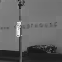
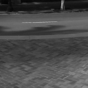
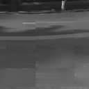
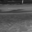
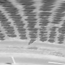
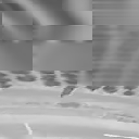
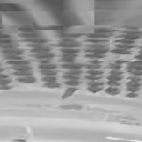
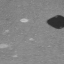
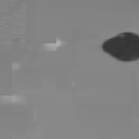
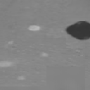
Fig. 10 presents sections of the inter predicted frames for VTM-14.2 and the proposed MPA with MPA-MVP=ON. For reference, the according sections from the original frames are shown as well. It is clearly visible that MPA is able to retain textures at a higher level of detail with less distracting blocking artifacts than VTM-14.2 is able to.

In Fig. 10(a) - (c), the text appears completely blurred in the inter predicted frame for VTM-14.2, while most letters are still readable for MPA. In Fig. 10(d) - (f), the tile texture of the midlane surface is heavily blurred and shows notable blocking artifacts for VTM-14.2, whereas MPA retains a much more detailed texture and shows less blocking artifacts. In Fig. 10(g) - (i), the crop field close to the north pole of the frame shows strong blocking artifacts with notable blur, while MPA is able to retain a higher level of detail. In Fig. 10(j) - (l), the street texture as well as the white marks are barely visible for VTM-14.2, whereas MPA preserves these marks and shows a finer street texture. The clearly visible improvements in the quality of the inter predicted frames obtained by MPA explain the achieved rate savings.

IV-D Motion Model Assessment

Table IV shows the rate savings that are achieved by different 360-degree motion models with respect to VTM-14.2 based on WS-PSNR. The comparative motion models are abbreviated as 3DT for the 3D-translational motion model [11, 12], TAN for the tangential motion model [18], ROT for the rotational motion model [15, 16], GED for the geodesic motion model [17], and TAN+ROT for the combined tangential and rotational motion model [19]. All motion models are using the same tools and extensions as MPA as described in Section III-D with the exception of the adapted motion vector prediction described in Section III-C that is not available for the comparative motion models. To ensure a fair comparison, MPA-MVP is thus disabled for MPA as well. The global camera motion vector required by GED is provided as prior information.

Please note that most comparative 360-degree motion models have originally been introduced in the context of the HEVC video coding standard [2], which did not feature the 4- and 6-parameter affine motion models available in VVC. The available affine motion models could be one of the main reasons for the reduced rate savings of the comparative 360-degree motion models with respect to their original publications.

Overall, MPA shows the highest average rate savings of 0.90% with the closest competitor being GED with average rate savings of 0.68%. Out of the remaining motion models, only 3DT is able to obtain rate savings on average, whereas all other motion models lead to increases in rate. Comparing MPA to GED, it is visible that GED is able to outperform MPA on Landing2 and BranCastle2. While on Landing2, GED achieves notable further rate savings over MPA, for BranCastle2, the rate savings obtained by MPA and GED are close. On the other hand, on the sequences SkateboardInLot, Balboa, and Broadway, MPA is able to achieve significantly higher rate savings than GED showcasing its broad applicability for diverse motion characteristics.

TABLE IV: Comparison of BD-Rate with respect to VTM-14.2 for different 360-degree motion models based on WS-PSNR. To allow a fair comparison, MPA-MVP=OFF for MPA. Negative values (black) represent actual rate savings, positive values (red) represent increases in rate. Bold entries mark the hightest rate savings among the tested motion models.

	MPA	3DT [11] [12]	TAN [18]	ROT [15] [16]	GED [17]	TAN+ ROT [19]
SkateboardInLot	-1.06	+0.13	+0.78	+0.79	-0.13	+0.88
ChairliftRide	-1.22	-0.16	+0.10	+0.42	-1.19	+0.13
KiteFlite	+0.03	+0.08	+0.06	-0.02	+0.05	+0.29
Harbor	+0.27	+0.16	+0.31	+0.07	+0.13	+0.15
Trolley	+0.04	+0.16	-0.02	+0.23	+0.15	-0.04
GasLamp	-0.08	-0.10	-0.74	-0.47	-0.57	-0.64
Balboa	-1.87	-0.07	+0.59	+0.71	-0.53	+0.59
Broadway	-1.64	+0.11	+0.78	+0.50	-0.61	+0.52
Landing2	-2.92	-1.03	-1.72	+0.25	-3.50	-0.99
BranCastle2	-0.58	-0.22	+0.03	+0.18	-0.62	+0.15
Average	-0.90	-0.09	+0.02	+0.27	-0.68	+0.10

IV-E Tool Utilization

((a)) Landing2, Frame 14, QP22, MPA-MVP=OFF

((b)) Landing2, Frame 14, QP22, MPA-MVP=ON

((c)) ChairliftRide, Frame 20, QP27, MPA-MVP=OFF

((d)) ChairliftRide, Frame 20, QP27, MPA-MVP=ON

Figure 11: MPA-CUs with motion planes color-coded as front/back (red), left/right (green), bottom/top (blue).

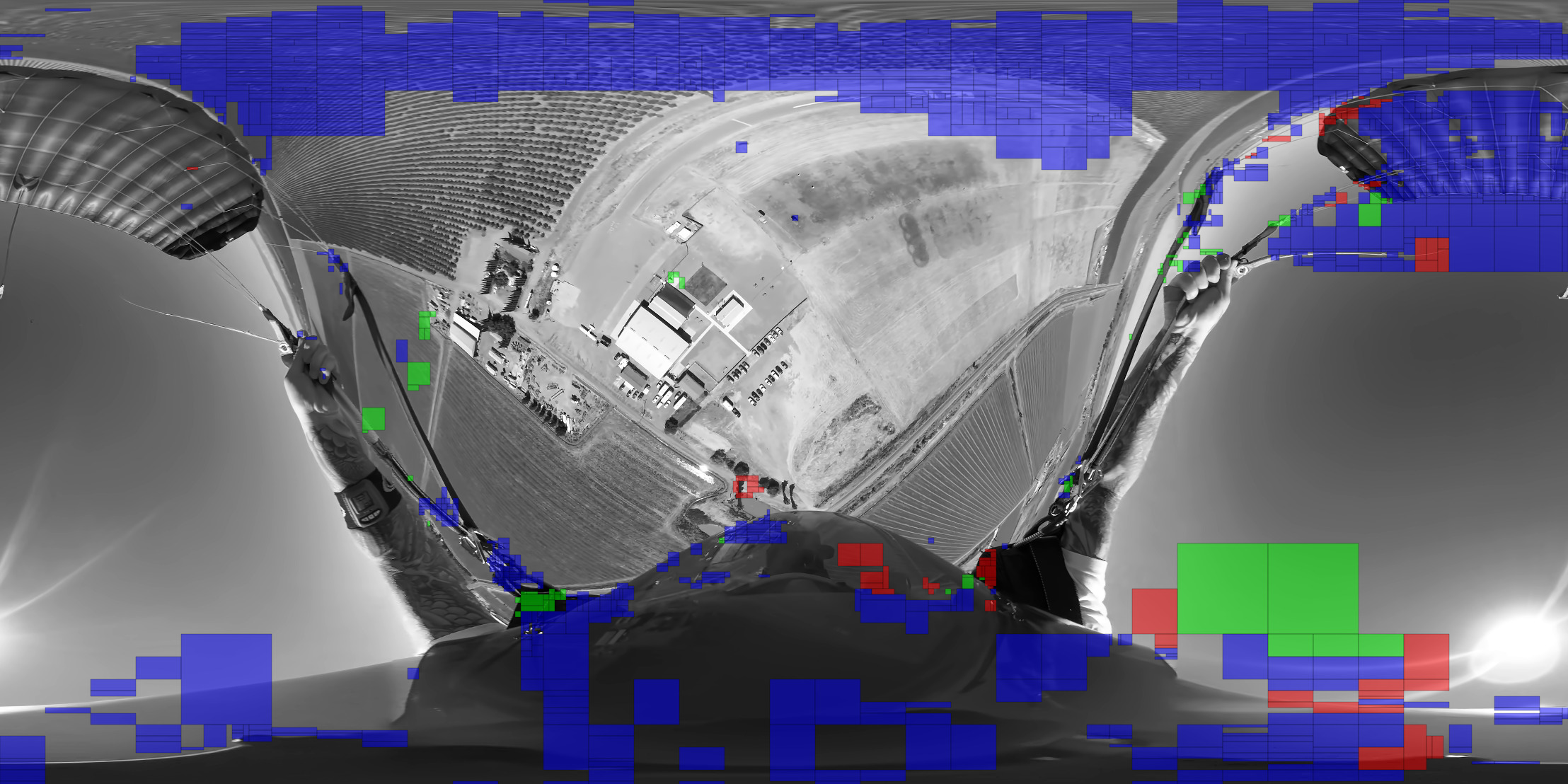
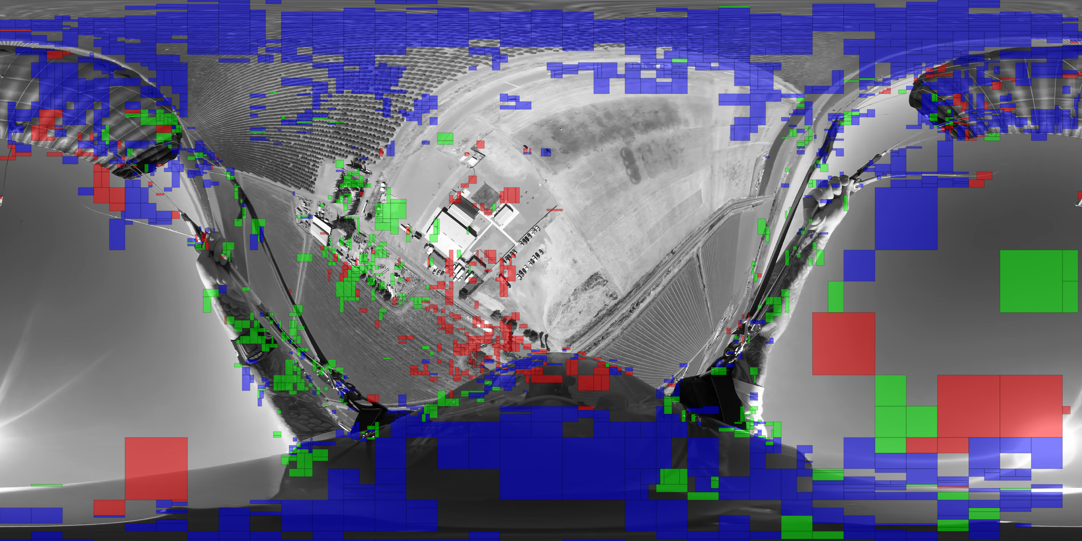
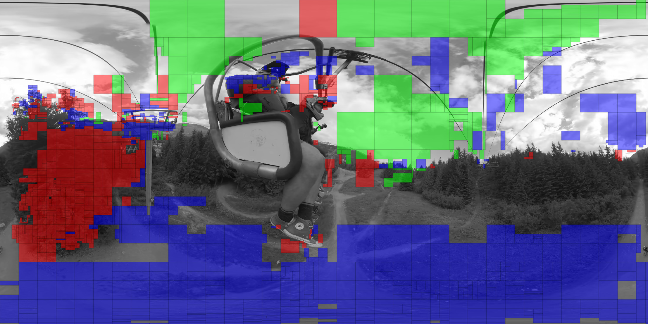
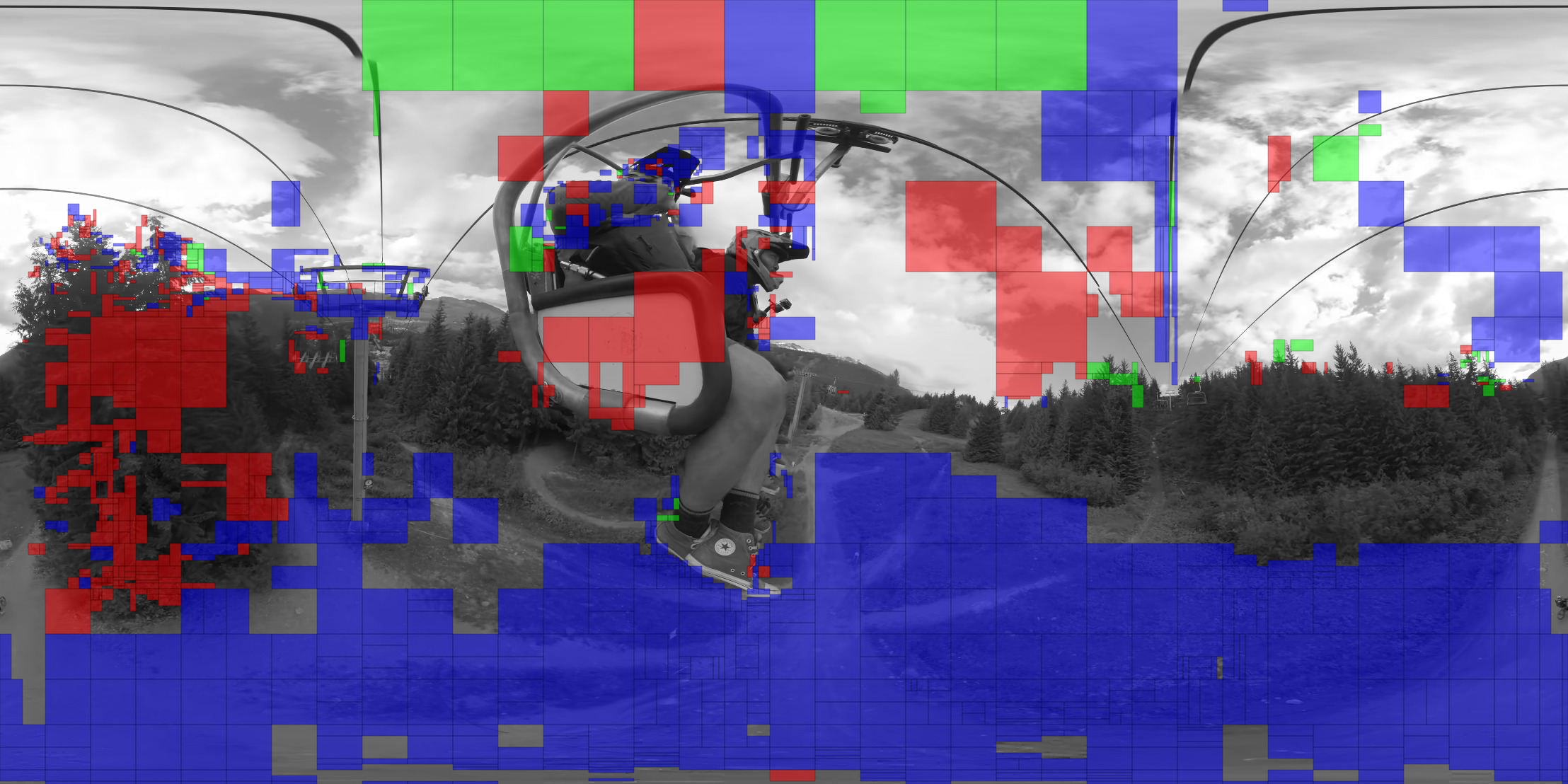
Table V displays the MPA-utilization as the average percentage of pixels predicted using the proposed MPA tool for each sequence for MPA-MVP=OFF and ON. The average utilization of MPA lies at 4.95% for MPA-MVP=OFF and at 5.76% for MPA-MVP=ON. While most sequences show an even higher MPA-utilization of more than 6% and 7% for MPA-MVP=OFF and ON, respectively, the four sequences KiteFlite, Harbor, Trolley and Gaslamp lie considerable below the average. As stated before, these sequences inhibit no global camera motion and only little, locally constrained object motion. The usage of MPA is therefore less prominent on these sequences as most CUs do not require an actual motion compensation at all.

TABLE V: Percentage of pixels predicted using MPA in MPA-VVC averaged over all frames.

MPA-MVP	OFF	ON
SkateboardInLot	6.86%	7.94%
ChairliftRide	10.38%	10.91%
KiteFlite	1.31%	1.39%
Harbor	1.00%	0.84%
Trolley	0.73%	0.65%
GasLamp	0.55%	0.60%
Balboa	7.30%	8.29%
Broadway	7.54%	8.80%
Landing2	6.22%	7.28%
BranCastle2	7.56%	10.94%
Average	4.95%	5.76%

Fig. 11 visualizes the motion plane maps, i.e., the motion plane decisions, for individual frames and QP values in the sequences Landing2 (Frame 14, QP=22) and ChairliftRide (Frame 20, QP=27) for MPA-MVP=ON and OFF. The motion plane decisions for each CU are color-coded as front/back (red), left/right (green) and bottom/top (blue). Transparent areas denote that another inter prediction tool or intra prediction is used.

In the motion plane maps for the sequence Landing2 in Fig. 11(a) and (b), the bottom/top motion plane is chosen especially in the highly distorted areas close to the north and south poles. The introduction of MPA-MVP in Fig. 11(b) shows clear benefits as the utilization of MPA towards the south pole increases notably compared to MPA-MVP=OFF in Fig. 11(a) and a lot of small, isolated CUs close the the center of the frame now employ MPA that previously used another tool. As the motion planes of MPA are not aligned with the motion surfaces for this sequence due to rich global camera translation and rotation, these observations show that MPA is able to better replicate the distortions occuring in 360-degree video than the classical translational and affine motion models even in suboptimal scenarios.

((a)) Decoder

((b)) Encoder

Figure 12: Boxplots visualizing the relative (a) decoder and (b) encoder complexity of the different motion models with respect to VTM-14.2. For MPA, the decoder and encoder complexity is shown for MPA-MVP=OFF (MPA) and ON (MPA+MPA-MVP). Furthermore, (b) shows a fast encoder configuration for MPA and MPA+MPA-MVP (hatched), where MPA is only enabled for CUs with a minimum size of 2048 pixels.

In the motion plane maps for the sequence ChairliftRide in Fig. 11(c) and (d), the motion surfaces in the sequence are better aligned with the available motion planes in MPA. As such, the bottom/top motion plane is selected for most of the CUs on the ground surface, matching the intuitive choice. Furthermore, the tree on the left of the image is coded using the front/back motion plane in many cases. As this region of the image actually lies ”behind” the camera in the spherical domain and the camera moves towards the right (along the cables), this choice can be intuitively expected, as well. While the impact of MPA-MVP is less prominent here, the considerably reduced cost of switching the motion plane or motion model is still clearly visible as MPA with MPA-MVP=ON in Fig. 11(d) is more flexible in the selection of the best suitable parameters for each CU compared to MPA-MVP=OFF in Fig. 11(c).

IV-F Complexity

Fig. 12(a) and (b) show boxplots representing the time complexity of the extended decoder and encoder for MPA and comparative 360-degree motion models with respect to the baseline VTM-14.2.

With a little more than 2-fold median complexity of MPA for MPA-MVP=OFF and slightly less than 2-fold complexity for MPA-MVP=ON with respect to VTM-14.2, the increase in decoder complexity as visible in Fig. 12(a) is on a similar level as other 360-degree motion models. However, as only GED showed convincing results in terms of rate-distortion performance (cf. Table IV), a comparison of MPA to GED is most expressive. With a median complexity of GED of a little more than 200% with respect to VTM-14.2, the overall decoding complexities of MPA and GED are similar. Nonetheless, the decoder for GED shows more extreme tendencies towards higher complexities with the third quartile lying at more than 400% compared to roughly 300% for MPA with MPA-MVP=OFF and ON. Maximum complexities reach up to 800% for GED and roughly 500% for MPA. Please note that further speed-ups can likely be achieved by runtime-optimized and/or hardware-specific implementations in the future.

However, with a median 25-fold complexity of MPA with MPA-MVP=OFF and 28-fold complexity of MPA with MPA-MVP=ON with respect to VTM-14.2, there is a significant increase in encoder complexity visible in Fig. 12(b). Other motion models mostly lie in the range from 5-fold to 10-fold complexity, where GED has outliers going up to almost 25-fold complexity and TAN+ROT has a roughly 17-fold complexity as both motion model configurations need to be checked. The increased encoder complexity for MPA with respect to other motion models is explicable by the motion estimation procedure needing to be performed three times for each of the available motion planes. Comparing the complexity of MPA-MVP=OFF versus ON, it is visible that the introduction of MPA-MVP only adds little to the complexity of the encoder. While the actual calculations required for MPA-MVP are negligible, MPA-MVP leads to more meaningful initializations of the motion vectors in the different motion models. This leads to motion estimation with greedy search strategies like the so-called test zone search implemented in VTM-14.2 running for more iterations until it stops, explaining the slight increase in complexity.

TABLE VI: Trade-off between obtained rate savings and relative encoder complexity for MPA with respect to VTM-14.2 based on WS-PSNR. Min CU defines the minimum number of pixels of a CU to allow the selection of the proposed MPA tool.

MPA-MVP	OFF		ON
Min CU	BD-Rate	Complexity	BD-Rate	Complexity
0	-0.90%	2617%	-1.56%	2851%
256	-1.15%	2191%	-1.39%	1749%
512	-1.00%	1703%	-1.35%	1327%
1024	-0.92%	829%	-1.16%	874%
2048	-0.76%	552%	-1.00%	610%
4096	-0.72%	434%	-0.83%	506%

Due to the high encoding complexity at hand, we looked into methods to speed up our proposed approach. Table VI shows results for a simple, yet effective, complexity reduction, where a minimum CU size is required in order to enable MPA. As expected, a trade-off between achieved rate savings (based on WS-PSNR) and complexity is adjustable via the minimum CU size. With a more than 4-fold reduction in complexity for a minimum CU size of 2048 pixels for MPA-MVP=ON compared to MPA without a CU size constraint, and retained rate savings of 1% on average, this simple technique demonstrates how a reduction of the search space can considerably speed up the encoding procedure. The hatched boxplots in Fig. 12(b) show that with this fast configuration, the encoding complexity of MPA is in a similar range as comparative 360-degree motion models. In future research, more sophisticated approaches and smart search strategies are therefore likely to achieve even higher speed-ups while keeping the good compression performance of MPA.

V Conclusion

In this paper, we proposed a novel motion-plane-adaptive inter prediction technique called MPA that allows inter prediction on different motion planes in 3D space. To let a video codec switch efficiently between different motion planes and motion models, we proposed a technique called MPA-MVP to translate motion information between them. Our proposed integration of MPA together with MPA-MVP in the state-of-the-art H.266/VVC video coding standard showed significant average rate savings of 1.72% based on PSNR and 1.56% based on WS-PSNR with respect to VTM-14.2 for the RA configuration, where the novel MPA-MVP contributes around 0.6% of the obtained rate savings on average. MPA showed to be among the most competitive 360-degree motion models with its closest competitor, i.e., the geodesic motion model [17], reaching average rate savings of 0.68% based on WS-PSNR.

In future research, we plan to investigate possibilities to reduce the complexity of MPA for both the encoder and the decoder by investigating optimized implementations for motion-plane-adaptive motion modeling and suitable fast encoder-side decision procedures. Furthermore, we plan to analyze the achievable rate savings if MPA is applied to other 360-degree projection formats.

References

- [1] T. Wiegand, G. Sullivan, G. Bjontegaard, and A. Luthra, “Overview of the H.264/AVC Video Coding Standard,” IEEE Trans. Circuits Syst. Video Technol., vol. 13, no. 7, pp. 560–576, Jul 2003.
- [2] G. J. Sullivan, J.-R. Ohm, W.-J. Han, and T. Wiegand, “Overview of the High Efficiency Video Coding (HEVC) Standard,” IEEE Trans. Circuits Syst. Video Technol., vol. 22, no. 12, pp. 1649–1668, Dec 2012.
- [3] B. Bross, J. Chen, J.-R. Ohm, G. J. Sullivan, and Y.-K. Wang, “Developments in International Video Coding Standardization After AVC, With an Overview of Versatile Video Coding (VVC),” Proc. IEEE, vol. 109, no. 9, pp. 1463–1493, Sep 2021.
- [4] B. Bross, Y.-K. Wang, Y. Ye, S. Liu, J. Chen, G. J. Sullivan, and J.-R. Ohm, “Overview of the Versatile Video Coding (VVC) Standard and its Applications,” IEEE Trans. Circuits Syst. Video Technol., vol. 31, no. 10, pp. 3736–3764, Oct 2021.
- [5] Y. Ye and J. Boyce, “Algorithm Descriptions of Projection Format Conversion and Video Quality Metrics in 360Lib Version 12, JVET-T2004-v2,” in Proc. 20th Meet. Jt. Video Expert. Team, Oct 2020, pp. 1–65.
- [6] M. Wien, V. Baroncini, P. Hanhart, J. Boyce, A. Segall, and T. Suzuki, “Results of the Call for Evidence on Video Compression with Capability beyond HEVC, JVET-G1004,” in Proc. 7th Meet. Jt. Video Explor. Team, Jul 2017, pp. 1–17.
- [7] Y. Ye, J. M. Boyce, and P. Hanhart, “Omnidirectional 360° Video Coding Technology in Responses to the Joint Call for Proposals on Video Compression With Capability Beyond HEVC,” IEEE Trans. Circuits Syst. Video Technol., vol. 30, no. 5, pp. 1241–1252, May 2020.
- [8] M. Hosseini and V. Swaminathan, “Adaptive 360 VR Video Streaming: Divide and Conquer,” in Proc. IEEE Int. Symp. Multimed., Dec 2016, pp. 107–110.
- [9] Y. S. de la Fuente, G. S. Bhullar, R. Skupin, C. Hellge, and T. Schierl, “Delay Impact on MPEG OMAF’s Tile-Based Viewport-Dependent 360° Video Streaming,” IEEE J. Emerg. Sel. Top. Circuits Syst., vol. 9, no. 1, pp. 18–28, Mar 2019.
- [10] G. Sullivan and T. Wiegand, “Rate-distortion optimization for video compression,” IEEE Signal Process. Mag., vol. 15, no. 6, pp. 74–90, Nov 1998.
- [11] L. Li, Z. Li, M. Budagavi, and H. Li, “Projection Based Advanced Motion Model for Cubic Mapping for 360-Degree Video,” in Proc. IEEE Int. Conf. Image Process., Sep 2017, pp. 1427–1431.
- [12] L. Li, Z. Li, X. Ma, H. Yang, and H. Li, “Advanced Spherical Motion Model and Local Padding for 360° Video Compression,” IEEE Trans. Image Process., vol. 28, no. 5, pp. 2342–2356, May 2019.
- [13] Y. Wang, L. Li, D. Liu, F. Wu, and W. Gao, “A New Motion Model for Panoramic Video Coding,” in Proc. IEEE Int. Conf. Image Process., Sep 2017, pp. 1407–1411.
- [14] Y. Wang, D. Liu, S. Ma, F. Wu, and W. Gao, “Spherical Coordinates Transform-Based Motion Model for Panoramic Video Coding,” IEEE J. Emerg. Sel. Top. Circuits Syst., vol. 9, no. 1, pp. 98–109, Mar 2019.
- [15] B. Vishwanath, T. Nanjundaswamy, and K. Rose, “Rotational Motion Model for Temporal Prediction in 360 Video Coding,” in Proc. IEEE 19th Int. Work. Multimed. Signal Process., Oct 2017, pp. 1–6.
- [16] B. Vishwanath, K. Rose, Y. He, and Y. Ye, “Rotational Motion Compensated Prediction in HEVC Based Omnidirectional Video Coding,” in Proc. Pict. Coding Symp., Jun 2018, pp. 323–327.
- [17] B. Vishwanath, T. Nanjundaswamy, and K. Rose, “Motion Compensated Prediction for Translational Camera Motion in Spherical Video Coding,” in Proc. IEEE 20th Int. Work. Multimed. Signal Process., Aug 2018, pp. 1–4.
- [18] F. De Simone, P. Frossard, N. Birkbeck, and B. Adsumilli, “Deformable Block-Based Motion Estimation in Omnidirectional Image Sequences,” in Proc. IEEE 19th Int. Work. Multimed. Signal Process., Oct 2017, pp. 1–6.
- [19] A. Marie, N. Mahmoudian Bidgoli, T. Maugey, and A. Roumy, “Rate-Distortion Optimized Motion Estimation for on-the-Sphere Compression of 360 Videos,” in Proc. IEEE Int. Conf. Acoust. Speech Signal Process., Jun 2021, pp. 1570–1574.
- [20] J. Sauer, J. Schneider, and M. Wien, “Improved Motion Compensation for 360° Video Projected to Polytopes,” in Proc. IEEE Int. Conf. Multimed. Expo, Jul 2017, pp. 61–66.
- [21] Y. He, Y. Ye, P. Hanhart, and X. Xiu, “Motion Compensated Prediction with Geometry Padding for 360 Video Coding,” in Proc. IEEE Vis. Commun. Image Process., Dec 2017, pp. 1–4.
- [22] J. Sauer, M. Wien, J. Schneider, and M. Blaser, “Geometry-Corrected Deblocking Filter for 360° Video Coding using Cube Representation,” in Proc. Pict. Coding Symp., Jun 2018, pp. 66–70.
- [23] C. Herglotz, M. Jamali, S. Coulombe, C. Vazquez, and A. Vakili, “Efficient Coding of 360° Videos Exploiting Inactive Regions in Projection Formats,” in Proc. IEEE Int. Conf. Image Process., Sep 2019, pp. 1104–1108.
- [24] Y. Zhou, L. Tian, C. Zhu, X. Jin, and Y. Sun, “Video Coding Optimization for Virtual Reality 360-Degree Source,” IEEE J. Sel. Top. Signal Process., vol. 14, no. 1, pp. 118–129, Jan 2020.
- [25] A. Regensky, C. Herglotz, and A. Kaup, “A Novel Viewport-Adaptive Motion Compensation Technique for Fisheye Video,” in Proc. IEEE Int. Conf. Acoust. Speech Signal Process., Jun 2021, pp. 1565–1569.
- [26] B. Bross, J. Chen, S. Liu, and Y.-K. Wang, “Versatile Video Coding (Draft 10), JVET-T2001-v2,” in Proc. 20th Meet. Jt. Video Explor. Team, Aug 2020, pp. 1–521.
- [27] ITU/ISO/IEC, “VVC VTM Reference Software VTM-14.2,” 2021. [Online]. Available: https://vcgit.hhi.fraunhofer.de/jvet/VVCSoftware_VTM/-/tree/VTM-14.2
- [28] A. Browne, J. Chen, Y. Ye, and S. H. Kim, “Algorithm Description for Versatile Video Coding and Test Model 14 (VTM 14), JVET-W2002-v1,” in Proc. 23rd Meet. Jt. Video Explor. Team, Jul 2021, pp. 1–111.
- [29] D. Marpe, H. Schwarz, and T. Wiegand, “Context-Based Adaptive Binary Arithmetic Coding in the H.264/AVC Video Compression Standard,” IEEE Trans. Circuits Syst. Video Technol., vol. 13, no. 7, pp. 620–636, Jul 2003.
- [30] L. Li, H. Li, D. Liu, Z. Li, H. Yang, S. Lin, H. Chen, and F. Wu, “An Efficient Four-Parameter Affine Motion Model for Video Coding,” IEEE Trans. Circuits Syst. Video Technol., vol. 28, no. 8, pp. 1934–1948, Aug 2018.
- [31] K. Zhang, Y.-W. Chen, L. Zhang, W.-J. Chien, and M. Karczewicz, “An Improved Framework of Affine Motion Compensation in Video Coding,” IEEE Trans. Image Process., vol. 28, no. 3, pp. 1456–1469, Mar 2019.
- [32] P. Hanhart, J. Boyce, K. Choi, and J. Lin, “JVET Common Test Conditions and Evaluation Procedures for 360° Video, JVET-L1012,” in Proc. 12th Meet. Jt. Video Explor. Team, Oct 2018, pp. 1–7.
- [33] F. Bossen, J. Boyce, K. Sühring, X. Li, and V. Seregin, “VTM Common Test Conditions and Software Reference Configurations for SDR Video, JVET-T2010,” in Proc. 20th Meet. Jt. Video Expert. Team, Oct 2020, pp. 1–2.
- [34] G. Bjontegaard, “Calculation of Average PSNR Differences between RD-curves, VCEG-M33,” in Proc. 13th Meet. Video Coding Expert. Gr., Mar 2001, pp. 1–5.
- [35] ITU/ISO/IEC, “360Lib Software 360Lib-12.0,” 2020. [Online]. Available: https://jvet.hhi.fraunhofer.de/svn/svn_360Lib/tags/360Lib-12.0/