A Robot Web for Distributed Many-Device Localisation

Abstract

We show that a distributed network of robots or other devices which make measurements of each other can collaborate to globally localise via efficient ad-hoc peer-to-peer communication. Our Robot Web solution is based on Gaussian Belief Propagation on the fundamental non-linear factor graph describing the probabilistic structure of all of the observations robots make internally or of each other, and is flexible for any type of robot, motion or sensor. We define a simple and efficient communication protocol which can be implemented by the publishing and reading of web pages or other asynchronous communication technologies. We show in simulations with up to 1000 robots interacting in arbitrary patterns that our solution convergently achieves global accuracy as accurate as a centralised non-linear factor graph solver while operating with high distributed efficiency of computation and communication. Via the use of robust factors in GBP, our method is tolerant to a high percentage of faulty sensor measurements or dropped communication packets. Furthermore, we showcase that the system operates on real robots with limited onboard computational resources.

I Introduction

Figure 1: In the Robot Web, we assume that a set of robots move through space while using their sensors to observe each other. The circles represent the variables – where ${{\mathbf{v}}}_{t}^{\alpha}$ denotes a variable at timestamp $t$ which belongs to robot $\alpha$ –, and the squares are the factors. Robot $\gamma$ starts at timestamp 3 for clarity of visualisation. The full-factor graph for multi-robot localisation is used. Responsibility for storing and updating it is divided up between the multiple robots participating, as shown by the coloured regions separated by dotted lines. Each robot maintains its own pose variable nodes, odometry factors, and factors for the inter-robot measurements made by its sensors, and carries out continuous GBP on this graph fragment. Message passing across dotted line boundaries happens on an asynchronous and ad-hoc basis.

 

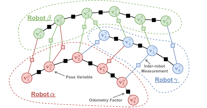
As we head towards a future where embodied artificial intelligence is ubiquitous, we expect that multiple robots, vehicles and other devices which share the same environment will need to communicate and coordinate their actions, whether their goal is explicit cooperation or just safe independent action. One clear possibility is that all devices could use a unified cloud-based ‘maps’ system, presumably owned by one company or government, which tracks and coordinates all devices. An alternative, which we investigate here, is a distributed system-based on per-device local computation and storage, and peer-to-peer communication between heterogeneous devices from different makers using standardised open protocols. Inspired by the original design of the World Wide Web, we call this concept the Robot Web.

A key outstanding problem in multi-robot systems has been true distributed localisation: how can a set of moving devices which move and observe each other within a space estimate their locations, using noisy actuators, sensors and realistic peer-to-peer communication?

In this paper, we present Robot Web, a solution to general, fully distributed and asynchronous many-robot localisation. Our solution is based on the fundamental probabilistic factor graph representation of perception and state estimation. We show that Gaussian Belief Propagation (GBP) [42] is the key inference algorithm with the appropriate properties of distributed processing/storage and message passing which permits a convergent, exact solution to the full, dynamically changing estimation problem via ad-hoc communication between robot peers.

In our solution, each robot stores and maintains its own part of the full factor graph (as shown in Figure 1), and updates and publishes a Robot Web Page of outgoing messages for other robots to download and read whenever possible. Remarkably, using GBP the whole factor graph can efficiently converge to localisation estimates as accurate as full batch optimisation but without any device ever needing to store or process more than its own local graph fragment. Robots communicate via ad-hoc, asynchronous messages containing only small vectors and matrices. Significantly, GBP can deal with graphs which have any type of parameterisation (e.g. 2D or 3D robot movement, or any type of non-linear sensor measurements) and which can change dynamically in arbitrary ways — for instance, robots can join or leave the web whenever needed, or reconfigure their sensors online. We will show that it can also cope with and reject a high fraction of outlier measurements, for instance, caused by faulty sensors, and deal with highly unreliable communication channels.

Our approach is designed for scalability. All communication is via a simple interface, and robots do not need any privileged information about each other, such as even how many other robots are involved. The whole Robot Web therefore can be fully dynamic, with robots joining or leaving at will. We believe that this formulation of many-robot localisation could be the foundation for a new era of distributed Spatial AI.

To summarise, the key contributions of our work are:

• A distributed, scalable localisation system based on Gaussian Belief Propagation (GBP) — Robot Web — that can localise thousands of robots in a simulated environment. Our method naturally handles asynchronous communication, communication failures, and a large number of outlier sensor measurements. Additionally, because all processing is local, our method can adapt to dynamic changes in the topology of the graph and handle disjoint connectivity.

• A framework for distributed multi-robot inference using GBP, and a novel extension of the GBP formulation to support Lie Groups, which is crucial for practical robotics applications.

• Extensive evaluation of our system to demonstrate the scalability. Using simulation, comparisons are made against a centralised counterpart across a range of parameters. Additionally, we have tested our system under challenging conditions, including the presence of a large number of non-Gaussian outlier sensor measurements and communication failures, in order to demonstrate its robustness.

• Real-time experiments with nine physical robots using only the limited computational resources available onboard. These experiments demonstrate the practicality and effectiveness of our approach and demonstrate that our method is feasible in real-world applications.

The rest of the paper is organised as follows. In Section II, we review previous work on multi-robot localisation and distributed localisation in sensor networks. In Section III, we provide an overview of GBP. Section IV extends the formulation of GBP to support Lie Groups, which is necessary for practical robotics applications which require state estimation for both translation and rotation. Section V describes our main contribution, which is a method for partitioning the factor graph across different devices and enabling communication between them. In Section VI, we present experimental results in a simulated environment and in Section VII with real robots. In Section VIII, we outline ongoing research topics. Finally, in Section IX, we conclude the paper and discuss potential directions for the future of distributed Spatial AI.

II Related Work

Robot Web uses the standard Gaussian factor graph representing the multi-robot localisation problem and is most closely related to the wealth of factor graph formulations and solvers in robotics, as well explained in the work of Dellaert and Kaess [20, 19]. Most methods for inference on factor graphs assume a centralised computer with access to the whole graph and focus on either efficient batch solution or incremental inference on graphs that are continually changing. Centralised pose-graph optimisation algorithms suitable for multiple robots are well-explored in the literature [27, 5, 30, 3]. MR-iSAM2 [55] extends iSAM2 [28] to build an incremental, centralised graph optimisation method for multiple robots. However, centralised methods require a base station, and are vulnerable to failure of this station, can require high communication bandwidth, create privacy concerns, and generally are not scalable [33].

There have been many previous attempts at distributed multi-robot localisation and SLAM which uses local computation and peer-to-peer communication, but these are generally far more limited or specific than Robot Web; there is a useful recent survey by Halsted et al. [25]. Leung et al. demonstrated that in a distributed network of robots, where the network is never fully connected, it is possible to achieve exact and centralised-equivalent estimates for localisation [36] and SLAM [35]. Many of the existing results in multi-robot SLAM perform a version of gradient descent, albeit in a distributed fashion [23]. A recent example is the work by Tian et al. [49] utilising block coordinate descent on the Riemannian manifold. The work by Tian et al. has also been used in Kimera-Multi [12] for pose-graph optimisation.

Other papers formulate the graph optimisation problem as a linear minimum mean-squared-error problem and utilise stationary iterative methods [24] such as the Jacobi method or the Gauss-Seidel method. For example, the Jacobi method is used by Barooah and Hespanha [7] and Aragues et al. [4] to solve the linearised system equations iteratively. The Jacobi method is implemented in a distributed manner as described in [21]. Choudhary et al. [13] demonstrates a distributed algorithm that scales to 50 robots. The algorithm utilises a distributed Gauss-Seidel method for solving linearised equations. This method has been used as a back-end optimisation module in other works such as DOOR-SLAM [32] and the recent work by Cieslewski et al. [14].

In DDF-SAM, Cunningham et al. [16] presented an algorithm that distributes factor graph optimisation across multiple robots. It relies on Gaussian elimination, and requires robots to exchange Gaussian marginals about shared variables. Later in DDF-SAM2 [15], an extension is proposed that avoids information double-counting. Similarly, the method presented in [34] involves robots exchanging condensed portions of their factor graphs in order to minimise communication. However, approaches which rely on Gaussian elimination become slow as the number of variables grows.

A significant limitation of the distributed methods above is that they are synchronous, which means the robots must share their messages at predetermined times to ensure the shared information is up-to-date. In contrast, asynchronous methods offer the flexibility that the robots can operate at their own rate, without waiting for other robots. Examples are the works by Todescato et al. [51] and Tian et al. [50]. The first reference conducts the optimisation in Euclidean space, while the latter does the optimisation by computing the gradient descent on a Riemannian manifold in a distributed manner. The authors of these papers also investigated the convergence of their distributed algorithms under communication delay.

Robot Web is also asynchronous and distributed, but both much more simple in formulation and more general than these methods. Significantly, Tian et al. [50] assume Gaussian noise are unable to handle outliers. Additionally, their formulation requires the sensor measurements to be a relative transformation. Robot Web supports general robot and sensor models and allows robust factors, making it robust to large fractions of non-Gaussian outlier measurements.

There has been some work on multi-agent distributed localisation using variations of belief propagation in the sensor networks community. For instance, Schiff et al. [46] performed multi-robot localisation using non-parametric belief propagation. Wymeersch et al. [54] also used belief propagation to perform cooperative positioning in a distributed manner. They used the sum-product algorithm over a factor graph in an ultra-wideband network. Then Caceres et al. [9] extended [54] to a network composed of GNSS nodes. These distributed positioning methods were later generalised by adding nonlinear measurement models and utilising Gaussian message passing [37], [38]; and in 2017, Wan et al. [52] proposed a distributed multi-robot SLAM algorithm, using belief propagation. In their method, a mixture of Gaussian and non-parametric models was used to handle nonlinear models. They also assumed measurements are affected by Gaussian noise and used synchronous message passing.

Robot Web goes far beyond these methods to present a general framework for general robots and sensors. It defines for the first time an open, asynchronous communication framework, and via the focus on GBP with robust factors enables highly robust and scalable performance.

III Gaussian Belief Propagation

A factor graph has a bipartite structure, composed of variable nodes and factor nodes. Variable nodes are only connected to factor nodes and vice versa.

GBP performs marginal inference, where it computes the per-variable marginal posterior distributions. The marginal inference proceeds iteratively via message passing between variable and factor nodes, which can in principle happen in many different types of patterns but still with convergent behaviour.

GBP is guaranteed to compute the exact marginal means on convergence, although the same is unfortunately not true for the variances as they are often overconfident for loopy graphs [53]. Thus when it converges, GBP yields the same mean as the maximum a posteriori (MAP) inference produced by a centralised solver. There are generally no convergence guarantees for GBP, but there are certain conditions under which it is known to converge and methods that can improve its chances of convergence [8].

This section summarises the basic operation of GBP. For more detailed derivation, refer to FutureMapping 2 [17] or ‘A visual introduction to Gaussian Belief Propagation’ [42].

We represent the Gaussian distribution in information form as:

$$\mathcal{N}({{\mathbf{x}}};{{\boldsymbol{\mu}}},{{\mathtt{\Sigma}}})=\mathcal{N}^{-1}({{\mathbf{x}}};{{\boldsymbol{\eta}}},{{\mathtt{\Lambda}}})~{},$$ (1)

where ${{\mathtt{\Lambda}}}={{\mathtt{\Sigma}}}^{-1}$ and ${{\boldsymbol{\eta}}}={{\mathtt{\Lambda}}}{{\boldsymbol{\mu}}}$. In GBP where we have $N_{v}$ variables and $N_{f}$ factors, variables $V=\{{{\mathbf{v}}}_{i}\}_{i=1:N_{v}}$ are assumed to be Gaussian; thus, each variable has a belief $b({{\mathbf{v}}}_{i})=\mathcal{N}^{-1}({{\mathbf{v}}}_{i};{{\boldsymbol{\eta}}}_{i},{{\mathtt{\Lambda}}}_{i})$. Factors $F=\{f_{i}\}_{i=1:N_{f}}$ are a probabilistic Gaussian constraint on or between the variables. We define neighbourhood $n({{\mathbf{x}}})$ to indicate the set of adjacent nodes connected via an edge to node ${{\mathbf{x}}}$ in the factor graph, where ${{\mathbf{x}}}$ may be a variable or a factor.

GBP can be divided into local operations at the variables, local operations at the factors, and message passing between them which we now detail.

III-A Variable Belief Update

The belief of a variable is the product of all the incoming messages:

$$b({{\mathbf{v}}}_{i})=\prod_{f\in n({{\mathbf{v}}}_{i})}{{\mathbf{m}}}_{f\rightarrow{{\mathbf{v}}}_{i}}({{\mathbf{v}}}_{i})~{},$$ (2)

where ${{\mathbf{m}}}_{f\rightarrow{{\mathbf{v}}}_{i}}({{\mathbf{v}}}_{i})=\mathcal{N}^{-1}({{\mathbf{v}}}_{i};{{\boldsymbol{\eta}}}_{f\rightarrow{{\mathbf{v}}}_{i}},{{\mathtt{\Lambda}}}_{f\rightarrow{{\mathbf{v}}}_{i}})$ is a message from a factor to a variable ${{\mathbf{v}}}_{i}$ along an edge.

III-B Variable to Factor Message

The message from a variable node ${{\mathbf{v}}}_{i}$ to a factor node $f_{j}\in n({{\mathbf{v}}}_{i})$ is computed as the product of all incoming messages from the neighbouring factor nodes of ${{\mathbf{v}}}_{i}$, except for the message from $f_{j}$. This can be expressed as:

$${{\mathbf{m}}}_{{{\mathbf{v}}}_{i}\rightarrow f_{j}}(f_{j})=\prod_{f\in n({{\mathbf{v}}}_{i})\backslash f_{j}}{{\mathbf{m}}}_{f\rightarrow{{\mathbf{v}}}_{i}}({{\mathbf{v}}}_{i})~{}.$$ (3)

III-C Factor Potential of Linear and Non-linear Function

The general definition of a Gaussian factor is:

$$f({{\mathbf{x}}};{{\mathbf{z}}}) = Ke^{-\frac{1}{2}\left[({{\mathbf{z}}}-{{\mathbf{h}}}({{\mathbf{x}}}))^{\top}{{\mathtt{\Lambda}}}_{s}({{\mathbf{z}}}-{{\mathbf{h}}}({{\mathbf{x}}}))\right]}$$ (4)

$$= Ke^{-E({{\mathbf{x}}};{{\mathbf{z}}})}~{},$$ (5)

where we have defined the general factor energy:

$$E({{\mathbf{x}}};{{\mathbf{z}}})=\frac{1}{2}({{\mathbf{z}}}-{{\mathbf{h}}}({{\mathbf{x}}}))^{\top}{{\mathtt{\Lambda}}}_{s}({{\mathbf{z}}}-{{\mathbf{h}}}({{\mathbf{x}}}))~{}.$$ (6)

This expression represents the probability of obtaining vector measurement ${{\mathbf{z}}}$ from the sensor as a function of the set of involved variables ${{\mathbf{x}}}$. Here, ${{\mathbf{h}}}$ is the functional form of the dependence of the measurement on state variables. Matrix ${{\mathtt{\Lambda}}}_{s}$ is the precision of the measurement. ${{\mathbf{x}}}$ represents the state space of all of the $N$ variables connected to the factor.

The general formula in Equation (4) for a factor represents a Gaussian distribution over the observed measurement ${{\mathbf{z}}}$. For linear measurement functions ${{\mathbf{h}}}({{\mathbf{x}}})$, the resulting linear factor is also a Gaussian distribution in the variables ${{\mathbf{x}}}$. To derive the Gaussian factor over ${{\mathbf{x}}}$, we begin with our general factor energy in Equation (6), and our goal is to manipulate the energy into the form of a Gaussian distribution over ${{\mathbf{x}}}$ in the information form:

$$E({{\mathbf{x}}};{{\mathbf{z}}})=\frac{1}{2}{{\mathbf{x}}}^{\top}{{\mathtt{\Lambda}}}{{\mathbf{x}}}-{{\boldsymbol{\eta}}}^{\top}{{\mathbf{x}}}~{}.$$ (7)

After transforming the energy into this form, we can identify the parameters ${{\boldsymbol{\eta}}}$ and ${{\mathtt{\Lambda}}}$ of the factor distribution.

To begin with, any linear measurement function can be generally written as:

$${{\mathbf{h}}}({{\mathbf{x}}})={{\mathtt{A}}}{{\mathbf{x}}}+{{\mathbf{b}}}~{},$$ (8)

where ${{\mathbf{b}}}\in\mathbb{R}^{m}$ is a constant vector and ${{\mathtt{A}}}\in\mathbb{R}^{m\times n}$ is a constant matrix for ${{\mathbf{z}}}\in\mathbb{R}^{m}$ and ${{\mathbf{x}}}\in\mathbb{R}^{n}$.

Substituting Equation (8) into the Equation (6) and rearranging:

$$E({{\mathbf{x}}};{{\mathbf{z}}}) = \frac{1}{2}\left[{{\mathbf{z}}}-{{\mathtt{A}}}{{\mathbf{x}}}-{{\mathbf{b}}}\right]^{\top}{{\mathtt{\Lambda}}}_{s}\left[{{\mathbf{z}}}-{{\mathtt{A}}}{{\mathbf{x}}}-{{\mathbf{b}}}\right]$$ (9)

$$= \frac{1}{2}\left[({{\mathbf{z}}}-{{\mathbf{b}}})-{{\mathtt{A}}}{{\mathbf{x}}}\right]^{\top}{{\mathtt{\Lambda}}}_{s}\left[({{\mathbf{z}}}-{{\mathbf{b}}})-{{\mathtt{A}}}{{\mathbf{x}}}\right]$$

$$= \frac{1}{2}\bigg{[}({{\mathbf{z}}}-{{\mathbf{b}}})^{\top}{{\mathtt{\Lambda}}}_{s}({{\mathbf{z}}}-{{\mathbf{b}}})+({{\mathtt{A}}}{{\mathbf{x}}})^{\top}{{\mathtt{\Lambda}}}_{s}{{\mathtt{A}}}{{\mathbf{x}}}$$

$$-({{\mathbf{z}}}-{{\mathbf{b}}})^{\top}{{\mathtt{\Lambda}}}_{s}{{\mathtt{A}}}{{\mathbf{x}}}-({{\mathtt{A}}}{{\mathbf{x}}})^{\top}{{\mathtt{\Lambda}}}_{s}({{\mathbf{z}}}-{{\mathbf{b}}})\bigg{]}~{}.$$

The first of the four terms here is a constant which doesn’t depend on ${{\mathbf{x}}}$ and so we can drop it into the normalising constant. The third and fourth are equal (one is the transpose of the other, and both are scalars), so we can simplify to:

$$E({{\mathbf{x}}};{{\mathbf{z}}}) = \frac{1}{2}({{\mathtt{A}}}{{\mathbf{x}}})^{\top}{{\mathtt{\Lambda}}}_{s}{{\mathtt{A}}}{{\mathbf{x}}}-({{\mathbf{z}}}-{{\mathbf{b}}})^{\top}{{\mathtt{\Lambda}}}_{s}{{\mathtt{A}}}{{\mathbf{x}}}$$ (10)

$$= \frac{1}{2}{{\mathbf{x}}}^{\top}({{\mathtt{A}}}^{\top}{{\mathtt{\Lambda}}}_{s}{{\mathtt{A}}}){{\mathbf{x}}}-\big{(}{{\mathtt{A}}}^{\top}{{\mathtt{\Lambda}}}_{s}({{\mathbf{z}}}-{{\mathbf{b}}})\big{)}^{\top}{{\mathbf{x}}}~{}.$$

Matching this with the Equation (7), we can identify the Gaussian information form parameters of the linear factor as:

$${{\boldsymbol{\eta}}}_{f} = {{\mathtt{A}}}^{\top}{{\mathtt{\Lambda}}}_{s}({{\mathbf{z}}}-{{\mathbf{b}}}),$$ (11)

$${{\mathtt{\Lambda}}}_{f} = {{\mathtt{A}}}^{\top}{{\mathtt{\Lambda}}}_{s}{{\mathtt{A}}}~{}.$$ (12)

For a non-linear measurement function ${{\mathbf{h}}}({{\mathbf{x}}})$, we can use a first-order Taylor expansion to linearize it around a reference point ${{\mathbf{x}}}_{0}$: ${{\mathbf{h}}}({{\mathbf{x}}})\approx{{\mathbf{h}}}({{\mathbf{x}}}_{0})+{{\mathtt{J}}}({{\mathbf{x}}}-{{\mathbf{x}}}_{0})$, where ${{\mathtt{J}}}$ is the Jacobian matrix of ${{\mathbf{h}}}({{\mathbf{x}}})$ with respect to ${{\mathbf{x}}}$ evaluated at ${{\mathbf{x}}}_{0}$. Rearranging and then matching, we get: ${{\mathtt{A}}}={{\mathtt{J}}}$ and ${{\mathbf{b}}}={{\mathbf{h}}}({{\mathbf{x}}}_{0})-{{\mathtt{J}}}{{\mathbf{x}}}_{0}$. Hence, the factor potential of a non-linear measurement function is:

$${{\boldsymbol{\eta}}}_{f} = {{\mathtt{J}}}^{\top}{{\mathtt{\Lambda}}}_{s}({{\mathbf{z}}}-({{\mathbf{h}}}({{\mathbf{x}}}_{0})-{{\mathtt{J}}}{{\mathbf{x}}}_{0}))~{},$$ (13)

$${{\mathtt{\Lambda}}}_{f} = {{\mathtt{J}}}^{\top}{{\mathtt{\Lambda}}}_{s}{{\mathtt{J}}}~{}.$$ (14)

III-D Factor to Variable Message

Let $V_{f}=n(f)$, a set of neighbouring variable nodes to factor $f$. To compute factor to variable messages, we take the product of the factor potential and messages from $V_{f}$, except for ${{\mathbf{v}}}_{i}$ before marginalising out $V_{f}\backslash{{\mathbf{v}}}_{i}$:

$${{\mathbf{m}}}_{f\rightarrow{{\mathbf{v}}}_{i}}({{\mathbf{v}}}_{i})=\sum_{V_{f}\backslash{{\mathbf{v}}}_{i}}f(V_{f})\prod_{{{\mathbf{v}}}_{j}\in V_{f}\backslash{{\mathbf{v}}}_{i}}{{\mathbf{m}}}_{{{\mathbf{v}}}_{j}\rightarrow f}({{\mathbf{v}}}_{j})~{}.$$ (15)

III-E Robust Factors

A common misunderstanding among roboticists is that loopy GBP is not a useful algorithm because uncertainty gating for data association is not possible due to overconfident covariance. A little consideration of any particular variable in the graph at convergence explains why we can in fact do properly-formulated data association using GBP. For a variable, we calculate its marginal belief by multiplying the probability distributions from the latest messages from all the factors it connects to. The fact that the marginal mean is correct for all variables at convergence shows that the relative precisions of local messages into a variable are convergently correct. This is what is important for data association — to be able to judge multiple hypotheses represented by different factors in the graph against each other.

We use robust factors on inter-robot measurements, and our approach can straightforwardly deal with a high fraction of non-Gaussian outlier sensor measurements. These outlier measurements do not need to be identified or dealt with in any explicit manner, but are simply automatically down-weighted by the robust factors and end up having a negligible influence on the whole graph. Note that this is a kind of ‘lazy data association’ because GBP’s final commitment to whether to accept a measurement can often happen some time after the measurement is reported, or could even be reversed later on if other supporting measurements arrive.

Specifically, using all of the latest incoming messages at a factor, we can compute the current potential at that factor, and interpret this as a Mahalanobis distance which indicates the ‘energy’ of the factor in terms of how many standard deviations away from its most probable value the current states of the variables are. This can be used for visualisation (to see which factors in a network are currently the most ‘stretched’ during optimisation), or for applying the effect of a robust kernel to downweight its effect.

At a factor, we combine the latest states of all the connected variables to form a stacked state representation ${{\mathbf{x}}}_{0}$. This acts as a linearisation point, and is used to compute the current Mahalanobis distance of the factor:

$$M=\sqrt{({{\mathbf{z}}}-{{\mathbf{h}}}({{\mathbf{x}}}_{0}))^{\top}{{\mathtt{\Lambda}}}({{\mathbf{z}}}-{{\mathbf{h}}}({{\mathbf{x}}}_{0}))}$$ (16)

Robust measurement functions in GBP can be handled by applying a robust scaling factor $k_{R}$ to the precision matrix and the information vector of the factor potential [17]:

$$\tilde{{\mathtt{\Lambda}}}^{\prime} = k_{R}{{\mathtt{\Lambda}}}^{\prime}$$ (17)

$$\tilde{{\boldsymbol{\eta}}}_{\mu} = k_{R}{{\boldsymbol{\eta}}}_{\mu}~{}.$$ (18)

This scaling factor depends on the Mahalanobis distance and can implement any robust kernel such as Huber, Tukey or DCS [1]. Through this mechanism, a factor will weaken itself by the appropriate probabilistic amount when the combination of variables it connects to means that the measurement the factor represents is likely to be an outlier. Overall, when many robust factors are connected in a large factor graph, GBP is able to use this mechanism to achieve lazy, reversible data association. We will see the impact of this in our results later in Section VI-D, where we show that we are able to deal with a large proportion of incorrect measurements in multi-robot localisation.

III-F Gaussian Belief Propagation for Multi-Device Distributed Inference

Extending GBP to the multi-device system is straightforward. Since GBP is a node-wise distributed algorithm and it operates via message passing, centralised GBP and distributed GBP are identical under perfect communication. No changes to the core algorithm is required for distributed inference.

As shown in Figure 1, we separate the nodes of the graph amongst the robots. At each iteration, we perform the following steps:

III-F1 Message Computation

Locally on each of the robots, variable-to-factor messages are computed using Equation (3), and the factor-to-variable messages are computed using Equation (15).

III-F2 Message Exchange

Messages are exchanged internally within a robot and externally between robots. An internal message is a message which is exchanged between nodes that belong to the same local graph, and an external message is a message which is sent from one robot to another via some communication mechanisms. To explain the external message passing more concretely, we use Robot $\alpha$ and Robot $\beta$ from Figure 1 as an example. The factors of Robot $\alpha$ will send factor-to-variable messages to ${{\mathbf{v}}}_{1}^{\beta}$, ${{\mathbf{v}}}_{2}^{\beta}$, and variable-to-factor messages from ${{\mathbf{v}}}_{2}^{\alpha}$, ${{\mathbf{v}}}_{3}^{\alpha}$ together with its point-estimate $\mu_{{{\mathbf{v}}}_{2}^{\alpha}}$, $\mu_{{{\mathbf{v}}}_{3}^{\alpha}}$ as the linearisation point. Both factor-to-variable and variable-to-factor messages are a marginal distribution, which is a $N\times 1$ vector and a $N\times N$ precision matrix for the message to or from a variable with $N$ degrees of freedom. Similarly, Robot $\beta$ will send Robot $\alpha$ the factor-to-variable messages to ${{\mathbf{v}}}_{2}^{\alpha}$, ${{\mathbf{v}}}_{3}^{\alpha}$, and variable-to-factor messages from ${{\mathbf{v}}}_{1}^{\beta}$, ${{\mathbf{v}}}_{2}^{\beta}$ with its point-estimate means.

III-F3 Variable Belief Update

Once messages are exchanged, the beliefs of the variables are updated via Equation (2), and we repeat this process until convergence.

We cover the specifics of how Robot Web partitions the factor graph, the communication model, and how the robots discover other robots’ factors later in Section V.

IV Gaussian Belief Propagation Inference with Lie Groups

It is possible to use Robot Web in vector space with no modification to the GBP as introduced in Section III. However, in most realistic robotics problems, there are additional details to consider due to the state space being a robot pose with rotation and translation, where careful thought about parameterisation is needed. The use of Lie theory is a key component of modern state estimation for robotics [6], and is applied to algorithms such as Extended Kalman Filter, and Information Filter [11].

In our work, we extend the four operations of GBP to support optimisation along a differentiable manifold, with a particular focus on Lie Groups, which is both a manifold and a group. We use concepts and the notation defined in Solà et al.’s excellent tutorial, ‘A micro Lie theory for state estimation in robotics’ [47].

First, we define two operations on the manifold: retraction $\mathcal{R}:\mathcal{M}\times T_{\mathcal{{\bar{X}}}}\mathcal{M}\rightarrow\mathcal{M}$, and its inverse $\mathcal{L}:\mathcal{M}\times\mathcal{M}\rightarrow T_{\mathcal{{\bar{X}}}}\mathcal{M}$, where $\mathcal{{\bar{X}}}\in\mathcal{M}$ is a point on a manifold $\mathcal{M}$, and $T_{\mathcal{{\bar{X}}}}\mathcal{M}$ is the tangent space of $\mathcal{M}$ at $\mathcal{{\bar{X}}}$. In case of a Lie Group we choose:

$$\mathcal{{\bar{Y}}} =\mathcal{R}(\mathcal{{\bar{X}}},{{\boldsymbol{\tau}}}) \triangleq\mathcal{{\bar{X}}}\oplus{{\boldsymbol{\tau}}} \triangleq\mathcal{{\bar{X}}}\circ\text{Exp}({{\boldsymbol{\tau}}})\in\mathcal{M}~{},$$ (19)

$${{\boldsymbol{\tau}}} =\mathcal{L}(\mathcal{{\bar{X}}},\mathcal{{\bar{Y}}}) \triangleq\mathcal{{\bar{Y}}}\ominus\mathcal{{\bar{X}}} \triangleq\text{Log}(\mathcal{{\bar{X}}}^{-1}\circ\mathcal{{\bar{Y}}})\in T_{\mathcal{{\bar{X}}}}\mathcal{M}~{},$$ (20)

where we use the Lie groups exponential and logarithmic map. For brevity, we focus on Lie Groups and will use its notation for the derivation.

Let $\mathcal{{\bar{X}}}$ represent the point estimate of a member of a Lie Group. A Gaussian distribution around this point estimate is represented using the tangent space as follows:

$$\mathcal{X}\sim\mathcal{N}(\mathcal{{\bar{X}}},{{\mathtt{\Lambda}}}^{-1})~{},$$ (21)

where:

$$\mathcal{X}=\mathcal{{\bar{X}}}\oplus\xi\\ ~{},\text{and}~{}\xi\sim\mathcal{N}(0,{{\mathtt{\Lambda}}}^{-1})~{}.$$ (22)

The core of how we use Lie Theory within GBP is the choice that all messages to or from a Lie Group variables take the form of a point estimate, represented by the full over-parameterised Group element, together with a minimal precision matrix defined in the tangent space around that element. So, when variable $\mathcal{X}$ represents a transformation which is a member of a Lie Group, all messages to it will take the form $\mathcal{{\bar{X}}},{{\mathtt{\Lambda}}}$, where ${{\mathtt{\Lambda}}}$ is a precision matrix in the tangent space at the point estimate $\mathcal{{\bar{X}}}$.

This approach gives maximum flexibility and minimises the need for independent devices to have knowledge or memory of each other (which might be required with alternative ideas, such as that messages would represent perturbations around some remembered stored element).

IV-A Belief Update at a Variable Node

At any stage, we can calculate a new marginal distribution at a variable node given all of the message passing that has happened to date; this is the current estimate of the position of a robot at a particular time step.

Consider a Lie Group variable connected to $N\geq 1$ factor nodes $i=1\ldots N$. In a message passing step, it must output a message to one of these factors, e.g. $i=a$. Each of the $N-1$ incoming messages has the form $\mathcal{{\bar{X}}}_{i},{{\mathtt{\Lambda}}}_{i}$; for each message, the precision matrix is in the local tangent space around the Lie Group element. We transform the tangent vector with its associated Gaussian distribution into the same tangent space, such that we can combine them. There are different possible choices for which tangent space to use, but a good choice is to use a previous estimate of the variable’s state $\mathcal{{\bar{X}}}_{0}$ (calculated the last time we did a belief update at that node; see Section IV-A) because this requires a minimal transformation of messages. To transform the mean of an incoming message into this tangent, space we perform:

$${{\boldsymbol{\tau}}}_{i}=\mathcal{{\bar{X}}}_{i}\ominus\mathcal{{\bar{X}}}_{0}~{}.$$ (23)

And to transform its precision matrix:

$${{\mathtt{\Lambda}}}_{{{\boldsymbol{\tau}}}_{i}}=\mathbf{J}^{\top}_{r}({{\boldsymbol{\tau}}}_{i}){{\mathtt{\Lambda}}}_{i}\mathbf{J}_{r}({{\boldsymbol{\tau}}}_{i})~{},$$ (24)

where $\mathbf{J}_{r}({{\boldsymbol{\tau}}})$, right Jacobian of $\mathcal{X}=\text{Exp}({{\boldsymbol{\tau}}})$, is:

$$\mathbf{J}_{r}({{\boldsymbol{\tau}}})=\lim_{\epsilon\rightarrow 0}\frac{\text{Exp}({{\boldsymbol{\tau}}}+\epsilon)\ominus\text{Exp}({{\boldsymbol{\tau}}})}{\epsilon}~{}.$$ (25)

To compute the belief at a variable, first, we sum all precision matrices to determine the total precision:

$${{\mathtt{\Lambda}}}_{{{\boldsymbol{\tau}}}}=\sum^{N}{{{\mathtt{\Lambda}}}_{{{{\boldsymbol{\tau}}}}_{i}}}~{},$$ (26)

and combine the messages to obtain the total tangent vector:

$${{\boldsymbol{\tau}}}={{\mathtt{\Lambda}}}_{{{\boldsymbol{\tau}}}}^{-1}\sum^{N}{{{\mathtt{\Lambda}}}_{{{\boldsymbol{\tau}}}_{i}}}{{\boldsymbol{\tau}}}_{i}~{}.$$ (27)

Finally we apply this tangent vector to $\mathcal{{\bar{X}}}_{0}$ to obtain the group element which is the mean of the belief of the variable:

$$\mathcal{{\bar{X}}}=\mathcal{{\bar{X}}}_{0}\oplus{{\boldsymbol{\tau}}}~{},$$ (28)

and warp the total precision into the tangent space of the new $\mathcal{{\bar{X}}}$:

$${{\mathtt{\Lambda}}}_{\mathcal{{\bar{X}}}}=\mathbf{J}^{-\top}_{r}({{\boldsymbol{\tau}}}){{\mathtt{\Lambda}}}_{{{\boldsymbol{\tau}}}}\mathbf{J}^{-1}_{r}({{\boldsymbol{\tau}}})~{}.$$ (29)

IV-B Variable to Factor Message

Given the latest incoming messages $\mathcal{{\bar{X}}}_{i},{{\mathtt{\Lambda}}}_{i}$ at the variable and the previously calculated belief mean $\mathcal{{\bar{X}}}_{0}$, we transform all incoming messages into the tangent space of $\mathcal{{\bar{X}}}_{0}$ using Equation (23) and Equation (24) to obtain ${{\boldsymbol{\tau}}}_{i}$ and ${{\mathtt{\Lambda}}}_{{{\boldsymbol{\tau}}}_{i}}$. Now that all ${{\boldsymbol{\tau}}}_{i}$ and ${{\mathtt{\Lambda}}}_{{{\boldsymbol{\tau}}}_{i}}$ are defined in the tangent space of $\mathcal{{\bar{X}}}_{0}$, we can add all precision matrices to determine the total precision:

$${{\mathtt{\Lambda}}}_{a}=\sum_{i\neq a}^{N}{{{\mathtt{\Lambda}}}_{{{{\boldsymbol{\tau}}}}_{i}}}~{}.$$ (30)

Next we can combine the messages to obtain the tangent vector of the outgoing message:

$${{\boldsymbol{\tau}}}_{a}={{\mathtt{\Lambda}}}_{a}^{-1}\sum_{i\neq a}^{N}{{{\mathtt{\Lambda}}}_{{{\boldsymbol{\tau}}}_{i}}}{{\boldsymbol{\tau}}}_{i}~{}.$$ (31)

Finally we apply this tangent vector to $\mathcal{{\bar{X}}}_{0}$ to obtain the group element which is the mean of the outgoing message:

$$\mathcal{{\bar{X}}}_{a}=\mathcal{{\bar{X}}}_{0}\oplus{{\boldsymbol{\tau}}}_{a}~{},$$ (32)

and warp the total precision to the tangent space of $\mathcal{{\bar{X}}}_{a}$:

$${{\mathtt{\Lambda}}}_{\mathcal{{\bar{X}}}_{a}}=\mathbf{J}^{-\top}_{r}({{\boldsymbol{\tau}}}_{a}){{\mathtt{\Lambda}}}_{a}\mathbf{J}^{-1}_{r}({{\boldsymbol{\tau}}}_{a})~{}.$$ (33)

The outgoing message to factor $a$ is: $\mathcal{{\bar{X}}}_{a},{{\mathtt{\Lambda}}}_{\mathcal{{\bar{X}}}_{a}}$, together with its most recent point estimate $\mathcal{{\bar{X}}}_{0}$.

IV-C Factor Potential of a Lie Group Parameterised Function

Here, we consider the case where at least one of the connected variables represent a Lie Group. Now parts of ${{\mathbf{x}}}$ will be group elements rather than simple vectors, and messages to and from those variables take the form of group elements together with precision matrices in the tangent space of those elements.

We first use the most recent variable states from the incoming messages from all variables connected to the factor to form stacked state representation ${{\mathbf{x}}}_{0}$. For example, for a factor connected to one $\mathbb{R}^{2}$ and two $\mathbf{SE}(2)$ variables:

$${{\mathbf{x}}}_{0} = \left[\begin{array}[]{cc}\mathcal{{\bar{X}}}_{0}^{1}\\ \mathcal{{\bar{X}}}_{0}^{2}\\ \mathcal{{\bar{X}}}_{0}^{3}\end{array}\right]\in\langle\mathbb{R}^{2},\mathbf{SE}(2),\mathbf{SE}(2)\rangle~{},$$ (37)

where $\mathcal{{\bar{X}}}_{0}^{i}$ is the variable $i$’s state. We will use ${{\mathbf{x}}}_{0}$ as the linearisation point for the factor, and perform the calculations needed for message passing in the tangent space around this point.

Our measurement function ${{\mathbf{h}}}$ output and the observation may not be Euclidean vectors. Hence, we define an error term:

$${{\mathbf{e}}}({{\mathbf{x}}})={{\mathbf{z}}}\mathrel{\ooalign{$-$\cr\hss\lower 1.09793pt\hbox{\Bigmath\char 5\relax}\hss}}{{\mathbf{h}}}({{\mathbf{x}}})~{},$$ (38)

where we use the notation $\mathrel{\ooalign{$-$\cr\hss\lower 1.09793pt\hbox{\Bigmath\char 5\relax}\hss}}$ from [47], which is an operation on the composite manifold ($\ominus$ operation is applied to each block of composites separately). We linearise the non-linear error term ${{\mathbf{e}}}$ via a first-order Taylor expansion around ${{\mathbf{x}}}_{0}$:

$${{\mathbf{e}}}({{\mathbf{x}}}) \approx {{\mathbf{e}}}({{\mathbf{x}}}_{0})+{{\mathtt{J}}}({{\mathbf{x}}}\mathrel{\ooalign{$-$\cr\hss\lower 1.09793pt\hbox{\Bigmath\char 5\relax}\hss}}{{\mathbf{x}}}_{0})$$ (41)

$$= {{\mathbf{e}}}({{\mathbf{x}}}_{0})+{{\mathtt{J}}}{{\boldsymbol{\tau}}}~{}.$$ (42)

Here ${{\mathtt{J}}}$ is the Jacobian of the measurement function with respect to the compound tangent space:

$${{\mathtt{J}}}=\frac{\partial{{\mathbf{e}}}}{\partial{{\boldsymbol{\tau}}}}|_{{{\mathbf{x}}}={{\mathbf{x}}}_{0}}=\left(\begin{array}[]{ccc}\frac{\partial{{\mathbf{e}}}}{\partial{{\boldsymbol{\tau}}}_{1}}&\frac{\partial{{\mathbf{e}}}}{\partial{{\boldsymbol{\tau}}}_{2}}&\frac{\partial{{\mathbf{e}}}}{\partial{{\boldsymbol{\tau}}}_{3}}\end{array}\right)~{}.$$ (43)

Identifying that ${{\mathtt{A}}}={{\mathtt{J}}}$ and ${{\mathbf{b}}}={{\mathbf{e}}}({{\mathbf{x}}}_{0})$, and substituting into Equation  (11), (12):

$${{\boldsymbol{\eta}}}_{f} = {{\mathtt{J}}}^{\top}{{\mathtt{\Lambda}}}_{s}(0-{{\mathbf{e}}}({{\mathbf{x}}}_{0}))~{},$$ (44)

$${{\mathtt{\Lambda}}}_{f} = {{\mathtt{J}}}^{\top}{{\mathtt{\Lambda}}}_{s}{{\mathtt{J}}}~{}.$$ (45)

${{\mathbf{z}}}_{s}=0$ as it’s already included in the error term to handle the group elements.

IV-D Factor to Variable Message

Having linearised the factor, we can now perform message passing. Consider our example factor connected to one $\mathbb{R}^{2}$ and two $\mathbf{SE}(2)$ variables. The factors information vector and precision matrix are partitioned as follows:

$${{\boldsymbol{\eta}}}_{\mu} = \left(\begin{array}[]{c}{{\boldsymbol{\eta}}}_{\mu_{1}}\\ {{\boldsymbol{\eta}}}_{\mu_{2}}\\ {{\boldsymbol{\eta}}}_{\mu_{3}}\end{array}\right)$$ (49)

$${{\mathtt{\Lambda}}}^{\prime} = \left[\begin{array}[]{ccc}{{\mathtt{\Lambda}}}_{11}^{\prime}&{{\mathtt{\Lambda}}}_{12}^{\prime}&{{\mathtt{\Lambda}}}_{13}^{\prime}\\ {{\mathtt{\Lambda}}}_{21}^{\prime}&{{\mathtt{\Lambda}}}_{22}^{\prime}&{{\mathtt{\Lambda}}}_{23}^{\prime}\\ {{\mathtt{\Lambda}}}_{31}^{\prime}&{{\mathtt{\Lambda}}}_{32}^{\prime}&{{\mathtt{\Lambda}}}_{33}^{\prime}\end{array}\right]~{}.$$ (53)

If we choose the output variable to be the third variable, we need to first condition the factor on the incoming messages from variables 1 and 2 and then marginalise to achieve an output distribution over variable 3. Conditioning is achieved by adding as follows:

$${{\boldsymbol{\eta}}}_{C} = \left(\begin{array}[]{c}{{\boldsymbol{\eta}}}_{\mu_{1}}+{{\boldsymbol{\eta}}}_{1}\\ {{\boldsymbol{\eta}}}_{\mu_{2}}+{{\boldsymbol{\eta}}}_{2}\\ {{\boldsymbol{\eta}}}_{\mu_{3}}\end{array}\right)$$ (57)

$${{\mathtt{\Lambda}}}_{Cs}^{\prime} = \left[\begin{array}[]{ccc}{{\mathtt{\Lambda}}}_{{11}}^{\prime}+{{\mathtt{\Lambda}}}_{1}&{{\mathtt{\Lambda}}}_{{12}}^{\prime}&{{\mathtt{\Lambda}}}_{{13}}^{\prime}\\ {{\mathtt{\Lambda}}}_{{21}}^{\prime}&{{\mathtt{\Lambda}}}_{{22}}^{\prime}+{{\mathtt{\Lambda}}}_{2}&{{\mathtt{\Lambda}}}_{{23}}^{\prime}\\ {{\mathtt{\Lambda}}}_{{31}}^{\prime}&{{\mathtt{\Lambda}}}_{{32}}^{\prime}&{{\mathtt{\Lambda}}}_{{33}}^{\prime}\end{array}\right]~{},$$ (61)

where $({{\boldsymbol{\eta}}}_{i}$, ${{\mathtt{\Lambda}}}_{i})$ describe the incoming message $(\mathcal{{\bar{X}}}_{i},{{\mathtt{\Lambda}}}_{\mathcal{{\bar{X}}}_{i}}^{\prime})$ from variable $i$ in the tangent space of ${{\mathbf{x}}}_{0}$.

$${{\boldsymbol{\tau}}}_{i} = \mathcal{{\bar{X}}}_{i}\mathrel{\ooalign{$-$\cr\hss\lower 1.09793pt\hbox{\Bigmath\char 5\relax}\hss}}{{\mathbf{x}}}_{0}^{i}$$ (64)

$${{\mathtt{\Lambda}}}_{i}^{\prime} = \mathbf{J}^{\top}_{r}({{\boldsymbol{\tau}}}_{i}){{\mathtt{\Lambda}}}_{\mathcal{{\bar{X}}}_{i}}^{\prime}\mathbf{J}_{r}({{\boldsymbol{\tau}}}_{i})$$ (65)

$$\eta_{i} = {{\mathtt{\Lambda}}}_{i}^{\prime}{{\boldsymbol{\tau}}}_{i}~{}.$$ (66)

Here ${{\mathbf{x}}}_{0}^{i}$ represents the $i$th block in the composite.

To complete message passing, from this joint distribution we must marginalise to obtain a distribution $\mathcal{N}^{-1}({{\boldsymbol{\eta}}}_{3},{{\mathtt{\Lambda}}}_{3})$ over the output variable. Eustice et al. [22] give the formula for marginalising a general partitioned Gaussian state in the information form. If the joint distribution is:

$${{\boldsymbol{\eta}}} = \left(\begin{array}[]{c}{{\boldsymbol{\eta}}}_{\alpha}\\ {{\boldsymbol{\eta}}}_{\beta}\end{array}\right)$$ (69)

$${{\mathtt{\Lambda}}} = w~{},$$ (70)

then the marginal distribution over the variables $\alpha$, achieved by integrating over the variables $\beta$, is:

$${{\boldsymbol{\eta}}}_{M\alpha} = {{\boldsymbol{\eta}}}_{\alpha}-{{\mathtt{\Lambda}}}_{\alpha\beta}{{\mathtt{\Lambda}}}_{\beta\beta}^{-1}{{\boldsymbol{\eta}}}_{\beta}$$ (71)

$${{\mathtt{\Lambda}}}_{M\alpha} = {{\mathtt{\Lambda}}}_{\alpha\alpha}-{{\mathtt{\Lambda}}}_{\alpha\beta}{{\mathtt{\Lambda}}}_{\beta\beta}^{-1}{{\mathtt{\Lambda}}}_{\beta\alpha}~{}.$$ (72)

The distribution $\mathcal{N}^{-1}({{\boldsymbol{\eta}}}_{3},{{\mathtt{\Lambda}}}_{3})$ is still in the tangent space of the linearised factor, so finally we transform back to a Lie Group element with the information matrix in its own tangent space as follows to form the outgoing message $\mathcal{{\bar{X}}}_{o3},{{\mathtt{\Lambda}}}_{\mathcal{{\bar{X}}}_{o3}}$:

$${{\boldsymbol{\tau}}}_{3} = {{\mathtt{\Lambda}}}_{3}^{-1}{{\boldsymbol{\eta}}}_{3}$$ (73)

$$\mathcal{{\bar{X}}}_{o3} = \mathcal{{\bar{X}}}_{0}^{3}\oplus{{\boldsymbol{\tau}}}_{3}$$ (74)

$${{\mathtt{\Lambda}}}_{\mathcal{{\bar{X}}}_{o3}} = \mathbf{J}^{-\top}_{r}({{\boldsymbol{\tau}}}_{3}){{\mathtt{\Lambda}}}_{3}\mathbf{J}^{-1}_{r}({{\boldsymbol{\tau}}}_{3})~{}.$$ (75)

V Robot Web: Core Design and Structure

We will use the term ‘robot’ for any device involved in the Robot Web, but some of these could be beacons, sensor nodes, or any other type of participating entity, which could be moving or stationary.

V-A Partitioning of the Factor Graph

The fundamental structure of the Robot Web is the full probabilistic factor graph which represents the states of robots as variables and the measurements they make, or any other information which is available such as pose or smoothness priors, as factors. Determining estimates of the robot states is a matter of performing inference on this factor graph to produce marginal distributions over the variables. We will assume that all factors take the form of Gaussian functions of the involved state variables, and use Gaussian Belief Propagation as the mechanism for inference. Note that GBP supports robust (heavy-tailed) factors and non-linear measurement functions via the methods proposed in [17], and therefore this model is very broadly practically applicable. These are the same assumptions behind most centralised factor graph inference libraries, such as GTSAM [18], Ceres [2], and g2o [31].

The key concept of the Robot Web is to distribute responsibility for storing and updating the full-factor graph, by dividing it up between the robots taking part. Figure 1 illustrates this for an elementary case of three moving robots, each with internal odometry sensing and an outward-looking sensor able to make observations of the other robots. We use different colours to highlight the parts of the factor graph for which each robot is responsible, and refer to the different robots using different Greek alphabets. A Robot $\alpha$ stores:

• The set of variables ${{\mathbf{v}}}_{t}^{\alpha}$ representing its state at discrete times $t$. It could store a whole history of states or a finite window. Most commonly these states will be multi-dimensional variables which directly represent robot pose, though any other aspects of internal state could be included. We will discuss pose parametrisation in detail later in Section IV.

• The set of factors $f_{t}^{\alpha}$ or $f_{t,t+1}^{\alpha}$ representing internal, priors or proprioceptive measurements. Each of these factors connects to one or more of the robot’s own state variables. Common examples would be a unary factor representing a GPS pose measurement, or a binary factor connecting two temporally consecutive states representing an odometry or inertial measurement.

• A set of factors $g_{t}^{\alpha,\beta}$ representing exteroceptive measurements made by this robot of other robots. Specifically, factor $g_{t}^{\alpha,\beta}$ represents a measurement made by this robot $\alpha$ of another robot $\beta$ at time $t$. This factor connects one state variable ${{\mathbf{v}}}_{t}^{\alpha}$ from robot $\alpha$ with state variable ${{\mathbf{v}}}_{t}^{\beta}$ of robot $\beta$ at the corresponding time.

There is an important design choice here: factors representing inter-robot measurements are stored by the robot making the measurement. This is because the details of measurement factors depend on the type and calibration of the sensor involved, and in this way, those details only need to be known to the robot carrying the sensor. Note also that we assume for now that all robots have globally synchronised clocks for timestamping of measurements (though we will see that all computation and communication can be asynchronous).

The factor graph evolves and grows dynamically. At initialisation, a robot will have just one variable node. As it moves, and measures its own incremental motion with odometry or similar, it adds the appropriate variables and factors to its internal factor graph. GBP runs continuously on the robot’s internal factor graph, producing always-updating marginal distributions for each variable. The message passing pattern of GBP within a robot’s internal factor graph is not important but should be rapid and global enough to keep the graph fragment mostly close to convergence.

V-B Message Passing and Communication Model

When the robot uses an outward-looking sensor to make an observation of the relative location of another robot, it creates a factor for this measurement, connects it to its current live pose variable, and the factor takes part in local GBP. The other end of this factor will initially be unconnected, because the appropriate variable to attach it to is stored by another robot: the factor-to-variable edge crosses the ‘dotted line’ boundary (see Figure 1), separating factor graph fragments. When local GBP generates an outgoing message from this factor which crosses the dotted line, that message is made available to the other robot that needs it.

The key idea behind Robot Web is that its inter-robot communication model is flexible and does not require synchronous or bidirectional communication. Instead, each robot can broadcast information at its own rate, which is particularly useful in large-scale systems where synchronising communication across multiple robots can be a challenge. This is only possible as GBP can converge even with an arbitrary message schedule [42] meaning that the communication between robots can be completely asynchronous and ad-hoc, but the overall graph made up of many fragments will converge to the global estimates. Here, we detail how the robots communicate with each other in our work.

V-B1 Communication Model

The asynchronous nature of the communication allows for a variety of options for message delivery, such as the publish-subscribe model used in systems like ROS/ROS2, where devices broadcast messages and listen to topics of interest, or the pull model, where devices query each other for information. In our work, we do not assume that messages will always be delivered, and any loss of messages will only result in a possible decrease in localisation accuracy, rather than causing a deadlock or critical failure. Additionally, we stress that our approach does not involve any shared global information among the robots. Each robot only exchanges messages with the others and does not share sensor models, initialisation status, or even the number of robots participating in the optimisation process. This combination of asynchronous communication and lack of shared global information allows the system to function even if there are fewer communication rounds than the total number of robots.

V-B2 Inter-device Factor Discovery

In Robot Web, the connection over the inter-device factors is formed lazily. A factor is created when an observation occurs. However, it takes a few iterations of message passing before the factor can be linearised. Specifically, when Robot $\alpha$ observes Robot $\beta$ at timestamp $t$, a factor $g_{t}^{\alpha,\beta}$ is formed. As the observation is made by Robot $\alpha$, it owns the factor. Robot $\alpha$ publishes an empty message ${{\mathbf{m}}}_{g_{t}^{\alpha,\beta}\rightarrow{{\mathbf{v}}}_{t}^{\beta}}$. Upon Robot $\beta$ receiving the message, it will publish the message ${{\mathbf{m}}}_{{{\mathbf{v}}}_{t}^{\beta}\rightarrow g_{t}^{\alpha,\beta}}$ together with the linearisation point $\mathcal{{\bar{X}}}_{t}^{\beta}$. When Robot $\alpha$ receives this message, it linearises the factor and starts the optimisation process. In the succeeding rounds, Robot $\beta$ will receive a message from Robot $\alpha$ which it can use to refine its pose estimate.

As GBP performs operations locally and does not use global information (e.g. topology of the graph), this sequence of message exchange occurs asynchronously, and GBP continues optimising as it discovers new inter-device factor connections.

V-B3 Robot Web Page Interface

One of the main motivations for the design choices made in Robot Web is the desire for distributed scalability. By providing a uniform interface, the robots can be added to or removed from the Robot Web in a fully dynamic manner, or can freely change their internal methods or software as long as they maintain the same interface. The internal complexity of each robot’s processing may be slightly increased because of this, but this is a small price to pay for global scalability.

To achieve this goal, one potential approach is to use a simple Web protocol (e.g. HTTP) for all inter-robot communication, with each robot hosting outgoing messages as a Web page. This allows inter-robot communication to happen in arbitrary patterns and in a read-only style, which can contribute to the scalability and flexibility of the system.

VI Demonstrations and Experiments in a Simulated Environment

We present extensive simulation demonstrations of Robot Web localisation for the case of many robots with planar 2D motion and noisy odometry and inter-robot range-bearing measurements. Our simulation uses metric units and models an application like a warehouse setting where tens or hundreds of robots roam through an environment 100m across with randomly generated paths. Usually, we add a handful of known beacon landmarks to the environment, whose positions are known in advance to all robots, but are widely spread so that robot-landmark measurements are much less frequent than robot-robot measurements. The main role of the landmarks is to anchor the whole web to an absolute coordinate frame over long periods of operation.

Our simulation uses a fully distributed program structure equivalent to what could be achieved on a true multi-robot system.

VI-A Implementation Details

In our experiments, we run the robots in a square arena of width 100m with 10 known beacons where all robots move through 100 pose steps. All variable nodes in the current simulation are represented using $\mathbf{SE}(2)$, and three different factors are implemented:

Anchor Factor: If needed, we can use unary anchor factors which are priors on the poses of robots before they start moving. In most experiments, we use these factors to represent fairly well-known initial robot positions at the start of motion, though note that in Section VI-G we show that new robots can be added to an existing web without any pose priors.

An anchor factor is defined as ${{\mathbf{h}}}({{\mathbf{x}}})={{\mathbf{x}}}$ with measurement ${{\mathbf{z}}}\in\mathbf{SE}(2)$, which is the prior pose estimate. The uncertainty assigned to the anchor factors in our main experiments is: $\sigma_{x}=0.1$m, $\sigma_{y}=0.1$m, and $\sigma_{\theta}=0.01$ rad.

Odometry Factor: For robot odometry, a binary factor ${{\mathbf{h}}}({{\mathbf{x}}}_{1},{{\mathbf{x}}}_{2})={{\mathbf{x}}}_{1}\ominus{{\mathbf{x}}}_{2}$ with measurement ${{\mathbf{z}}}\in{\mathfrak{se}(2)}$ represents a relative pose measurement. The uncertainty assigned to odometry factors per metre step is: $\sigma_{x}=0.1$m, $\sigma_{y}=0.01$m, and $\sigma_{\theta}=0.01$ rad. As each robot moves along its x-axis, the uncertainty on $x$ is higher than $y$.

Range-Bearing Factor: We use a range-bearing sensor for the measurements between robots, or between robots and landmarks. The measurement function is ${{\mathbf{h}}}({{\mathbf{x}}}_{1},{{\mathbf{x}}}_{2})=(r,b)$, where $r$ is the Euclidean distance between ${{\mathbf{x}}}_{1},{{\mathbf{x}}}_{2}$ and $b$ is the angle between the ${{\mathbf{x}}}_{1},{{\mathbf{x}}}_{2}$ in the coordinate frame of ${{\mathbf{x}}}_{1}$. The range-bearing measurement is defined as $z\in\langle\mathbb{R},\mathbf{SO}(2)\rangle$. By default the uncertainty assigned to range/bearing factors is: $\sigma_{r}=0.01$m, $\sigma_{b}=0.05$ rad, with the sensor range limited to 30m. DSC [1] is used as the robust kernel with $\Phi=10$. Alongside the Gaussian noise, to 10% of all range-bearing measurements, we additionally add a huge amount of uniform noise: $r_{n}\sim\mathcal{U}(0,30)$, $b_{n}\sim\mathcal{U}(0,\pi)$ to simulate non-Gaussian noise which makes these measurements essentially useless.

We use a communication pattern which simulates a limited peer-to-peer communication budget, where each robot connects to and reads the Robot Web page from other robots in a sequential, random pattern with closer robots are more likely to be selected. The idea is that this is similar to a robot sequentially switching its Wi-Fi connection between peers with strong signals.

We generated a noisy distance sample between Robot $\alpha$ and Robot $\beta$ as $d_{\alpha,\beta}\sim\mathcal{N}({\bar{d}}_{\alpha,\beta},0.1)$, where $d_{\alpha,\beta}$ is the random sample and ${\bar{d}}_{\alpha,\beta}$ is the ground truth distance between Robot $\alpha$ and Robot $\beta$. We define the neighbourhood of $\alpha$, $N(\alpha)$, as the set of robots which Robot $\alpha$ can communicate with. The probability $C_{\alpha,\beta}$ that Robot $\alpha$ communicates with Robot $\beta\in N(\alpha)$ is:

$$p(C_{\alpha,\beta})=\frac{1/d_{\alpha,\beta}^{2}}{\sum_{\omega\in N(\alpha)}{1/d_{\alpha,\omega}^{2}}}~{}.$$ (76)

In this work, we assume that $N(\cdot)$ includes all robots. Each robot performs 20 iterations of GBP per movement step and at each GBP step robots communicate with only one neighbour. Factors are dampened [40] by 0.2, and the factors linearise at every iteration. Any changes to the default parameters will be specified in the individual experiments.

VI-B Convergence and Computational Properties

(a) Mean RMSE ATE

(b) Mean RMSE Translational RPE

(c) Mean RMSE Rotational RPE

Figure 2: In a simulated environment, N robots are moving around in an environment with 10 known landmarks for 100 poses each. GTSAM optimises the factor graph after every pose insertion rather than solving after all poses are inserted to keep the comparison fair. GBP uses the full factor graph to optimise, while Windowed GBP only uses only the last 5 poses. The results are the average of 10 runs with different random initialisation, and the error bar represents one standard deviation of uncertainty.

 

Figure 3: Increasing the number of iterations per step decreases the overall error. Even with a small number of iterations, GBP is able to provide good localisation, which can be further refined by increasing the iterations. The red line shows the median, the box extends from the first quartile to the third quartile, the whisker extends from the box by 1.5 inter-quartile range, and the outliers are marked with a cross. In a simulated environment, 50 robots are moving in an environment with 10 known landmarks for 100 poses each. Each result is a summary of 50 runs with different random initialisation.

 

TABLE I: The RMSE ATE of the trajectories for different numbers of robots in simulation. We report the mean error and the standard deviation of 10 runs with different random initialisation.

N	Range	Noise	GTSAM	GBP	Windowed
	[m]	[m, rad]	$\mu\pm\sigma$ [m]	$\mu\pm\sigma$ [m]	$\mu\pm\sigma$ [m]
16	10	0.01, 0.05	$0.660\pm 0.217$	$0.770\pm 0.183$	$0.934\pm 0.152$
	10	0.05, 0.1	$0.690\pm 0.218$	$0.773\pm 0.192$	$0.975\pm 0.127$
	30	0.01, 0.05	$0.063\pm 0.024$	$0.066\pm 0.025$	$0.088\pm 0.042$
	30	0.05, 0.1	$0.081\pm 0.019$	$0.087\pm 0.021$	$0.117\pm 0.040$
32	10	0.01, 0.05	$0.314\pm 0.062$	$0.462\pm 0.080$	$0.561\pm 0.076$
	10	0.05, 0.1	$0.344\pm 0.049$	$0.437\pm 0.058$	$0.597\pm 0.063$
	30	0.01, 0.05	$0.015\pm 0.003$	$0.016\pm 0.003$	$0.022\pm 0.008$
	30	0.05, 0.1	$0.035\pm 0.003$	$0.036\pm 0.004$	$0.043\pm 0.006$
64	10	0.01, 0.05	$0.154\pm 0.018$	$0.290\pm 0.072$	$0.358\pm 0.072$
	10	0.05, 0.1	$0.181\pm 0.023$	$0.256\pm 0.064$	$0.375\pm 0.080$
	30	0.01, 0.05	$0.009\pm 0.001$	$0.009\pm 0.001$	$0.010\pm 0.003$
	30	0.05, 0.1	$0.023\pm 0.001$	$0.023\pm 0.001$	$0.024\pm 0.003$
128	10	0.01, 0.05	$0.060\pm 0.004$	$0.105\pm 0.016$	$0.134\pm 0.015$
	10	0.05, 0.1	$0.082\pm 0.004$	$0.102\pm 0.009$	$0.158\pm 0.011$
	30	0.01, 0.05	$0.006\pm 0.000$	$0.006\pm 0.000$	$0.006\pm 0.000$
	30	0.05, 0.1	$0.016\pm 0.000$	$0.016\pm 0.000$	$0.016\pm 0.000$

TABLE II: The translational RMSE RPE of the trajectories for different numbers of robots in simulation. We report the mean error and the standard deviation of 10 runs with different random initialisation.

N	Range	Noise	GTSAM	GBP	Windowed
	[m]	[m, rad]	$\mu\pm\sigma$ [m]	$\mu\pm\sigma$ [m]	$\mu\pm\sigma$ [m]
16	10	0.01, 0.05	$0.321\pm 0.084$	$0.349\pm 0.071$	$0.382\pm 0.064$
	10	0.05, 0.1	$0.336\pm 0.082$	$0.356\pm 0.077$	$0.396\pm 0.064$
	30	0.01, 0.05	$0.087\pm 0.020$	$0.087\pm 0.019$	$0.090\pm 0.018$
	30	0.05, 0.1	$0.119\pm 0.025$	$0.118\pm 0.025$	$0.120\pm 0.025$
32	10	0.01, 0.05	$0.207\pm 0.028$	$0.235\pm 0.041$	$0.264\pm 0.048$
	10	0.05, 0.1	$0.227\pm 0.032$	$0.238\pm 0.034$	$0.276\pm 0.039$
	30	0.01, 0.05	$0.068\pm 0.015$	$0.068\pm 0.016$	$0.069\pm 0.016$
	30	0.05, 0.1	$0.102\pm 0.021$	$0.101\pm 0.021$	$0.102\pm 0.020$
64	10	0.01, 0.05	$0.164\pm 0.015$	$0.198\pm 0.031$	$0.216\pm 0.033$
	10	0.05, 0.1	$0.191\pm 0.015$	$0.197\pm 0.020$	$0.227\pm 0.030$
	30	0.01, 0.05	$0.054\pm 0.007$	$0.053\pm 0.006$	$0.053\pm 0.006$
	30	0.05, 0.1	$0.078\pm 0.009$	$0.077\pm 0.009$	$0.077\pm 0.009$
128	10	0.01, 0.05	$0.092\pm 0.009$	$0.105\pm 0.009$	$0.109\pm 0.009$
	10	0.05, 0.1	$0.120\pm 0.004$	$0.126\pm 0.003$	$0.135\pm 0.005$
	30	0.01, 0.05	$0.047\pm 0.002$	$0.047\pm 0.002$	$0.047\pm 0.002$
	30	0.05, 0.1	$0.068\pm 0.003$	$0.068\pm 0.003$	$0.068\pm 0.003$

TABLE III: The rotational RMSE RPE of the trajectories for different numbers of robots in simulation. We report the mean error and the standard deviation of 10 runs with different random initialisation.

N	Range	Noise	GTSAM	GBP	Windowed
	[m]	[m, rad]	$\mu\pm\sigma$ [deg]	$\mu\pm\sigma$ [deg]	$\mu\pm\sigma$ [deg]
16	10	0.01, 0.05	$0.626\pm 0.028$	$0.642\pm 0.025$	$0.776\pm 0.036$
	10	0.05, 0.1	$0.639\pm 0.031$	$0.650\pm 0.030$	$0.789\pm 0.033$
	30	0.01, 0.05	$0.510\pm 0.012$	$0.510\pm 0.012$	$0.528\pm 0.019$
	30	0.05, 0.1	$0.535\pm 0.012$	$0.535\pm 0.013$	$0.579\pm 0.015$
32	10	0.01, 0.05	$0.574\pm 0.011$	$0.592\pm 0.015$	$0.732\pm 0.034$
	10	0.05, 0.1	$0.589\pm 0.011$	$0.596\pm 0.012$	$0.750\pm 0.019$
	30	0.01, 0.05	$0.496\pm 0.007$	$0.496\pm 0.007$	$0.501\pm 0.007$
	30	0.05, 0.1	$0.519\pm 0.007$	$0.519\pm 0.007$	$0.545\pm 0.009$
64	10	0.01, 0.05	$0.549\pm 0.007$	$0.567\pm 0.013$	$0.695\pm 0.034$
	10	0.05, 0.1	$0.569\pm 0.009$	$0.573\pm 0.008$	$0.711\pm 0.029$
	30	0.01, 0.05	$0.475\pm 0.003$	$0.476\pm 0.003$	$0.477\pm 0.004$
	30	0.05, 0.1	$0.506\pm 0.003$	$0.506\pm 0.003$	$0.517\pm 0.003$
128	10	0.01, 0.05	$0.518\pm 0.004$	$0.523\pm 0.004$	$0.576\pm 0.006$
	10	0.05, 0.1	$0.540\pm 0.004$	$0.542\pm 0.004$	$0.614\pm 0.006$
	30	0.01, 0.05	$0.443\pm 0.004$	$0.443\pm 0.004$	$0.444\pm 0.004$
	30	0.05, 0.1	$0.490\pm 0.002$	$0.490\pm 0.002$	$0.495\pm 0.002$

A key property of our method is that the marginal estimates generated by message passing with a fixed computation and communication budget on our ever-changing factor graph may not necessarily be at complete convergence during live operation, though that is often not a problem if useful robot pose estimates are still achieved. Nevertheless, here we show that when enough computation and communication are regularly applied, the localisation results are convergent and estimates as accurate as a batch solution on a centralised processor can be achieved. Importantly, this can be achieved with highly efficient, realistic settings for distributed GBP computation and communication.

Here we present an experiment to compare the accuracy of distributed Robot Web GBP against a centralised solution of the same factor graph using GTSAM [19]. GBP linearises at every 5 iterations and is allowed to optimise for 20 iterations per step. To keep the comparison simple, robust kernels are not applied for both GBP and GTSAM, and we do not add uniform noise to the range-bearing measurements.

We present results for general GBP, where each robot keeps a full history of pose variables, and Windowed GBP, where each robot maintains a sliding window of its most recent 5 poses and only processes messages relating to these. Using a sliding window allows the average size of the factor graph, and the amount of computation needed, to remain fixed. This allows the system to operate over an arbitrarily long period while maintaining constant computational cost. What we lose by doing this is the possibility to improve estimates of older variables in the graph using new observations.

In these experiments, for both versions of GBP, all robots are allowed to communicate with each other on every iteration.

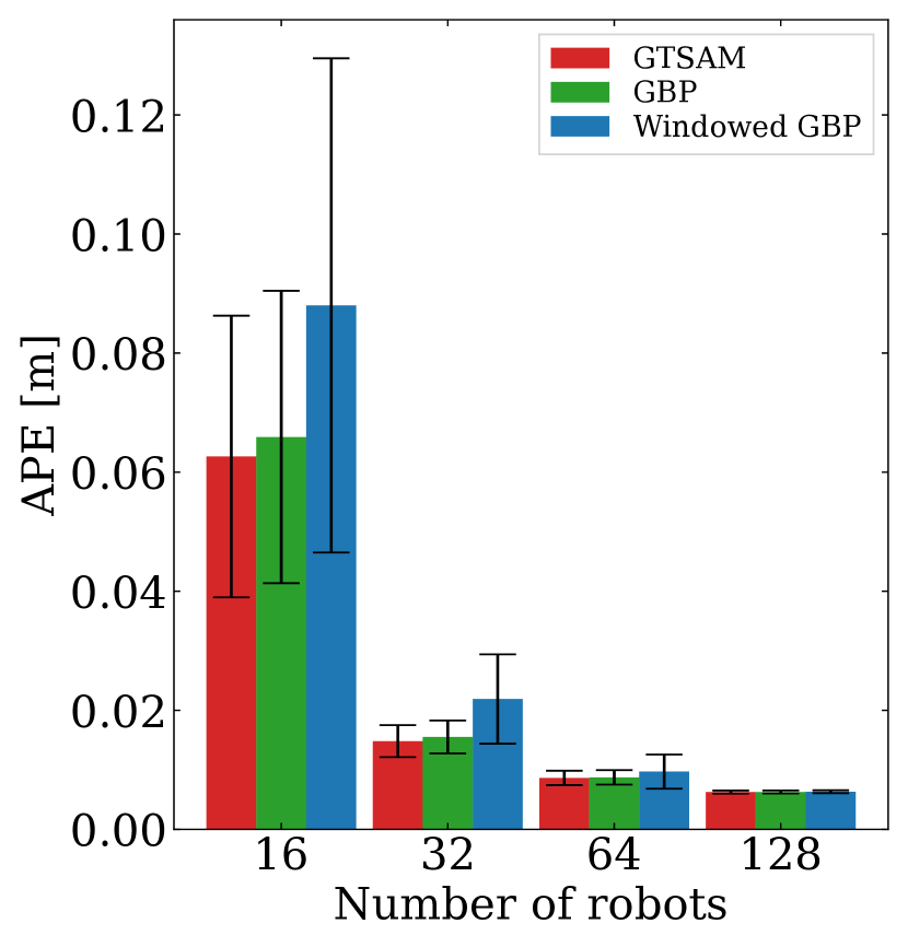
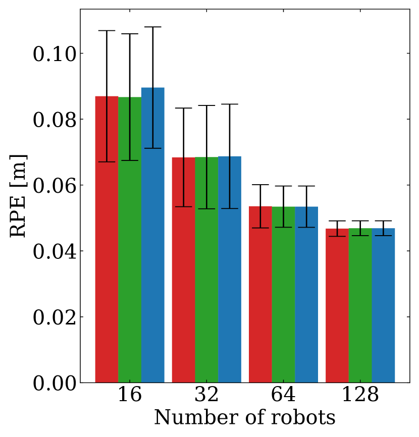
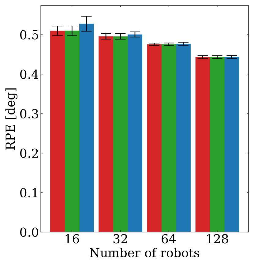
We report the Root Mean Square Absolute Trajectory Error (RMSE ATE), and Root Mean Square Relative Pose Error (RMSE RPE) [48], averaged over 10 runs with randomised robot motions in Figure 2, for varying numbers of robots in the area. Both ATE and RPE are computed over the full trajectory. We see that GBP and GTSAM have similar ATE across all evaluations, with only a small loss of accuracy for GBP when the number of robots is low.

As the number of robots increases, the difference in ATE across the different approaches becomes negligible. Windowed GBP reaches comparable accuracy to GTSAM and GBP, even with a significantly smaller computational cost when compared to full GBP optimisation.

A similar pattern is observed when we vary the sensor noise and range. As we increase the number of robots, the difference in error across different approaches reduces. The sensor noise is increased to $\sigma_{r}=0.05$m, $\sigma_{b}=0.1$ rad, and the range is limited to 10m. Table I, II, III summarises the result of sweeps over the different parameters.

When the sensor range is limited or the number of robots is small, fewer observations are made and robots will drift more from their correct trajectories. Being a local algorithm, GBP can rapidly optimise local, high-frequency component errors in the network [17], while it requires more iterations for information to propagate across the graph to optimise lower frequency component errors, such as longer drifts. This property is observable in Figure 2 where the difference in ATE between GTSAM and GBP for 16 robots is noticeable due to the low-frequency noise. Since the range of the sensors is limited, fewer observations are made when the total number of robots is small, as the arena has a lower density of robots. Similarly, as shown in Table I for N=128. When the sensor range is 30m, GTSAM and GBP achieve the same ATE. However, when the sensor range is 10m, a small difference exists. However; in both cases for the relative metric RPE, similar performance is achieved even with a small number of robots, demonstrating that the local/high-frequency component errors are correctly smoothened.

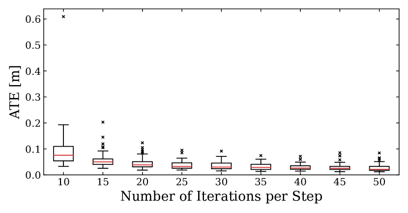
Increasing the number of iterations improves convergence as more messages are exchanged. We can verify this in Figure 3, where we vary the number of iterations per step between 10-50. We use 50 robots and report the average over 50 different runs. We see that as the number of iterations per step increases, ATE decreases; however, with diminishing returns. The optimal number of iterations per step depends on many factors (e.g. topology of the graph, communication pattern) and is an interesting direction for further research.

VI-C Operation with a Large Number of Agents

In terms of computational performance, it would not be meaningful to report the speed of our C++ CPU simulation of the Robot Web algorithm, which is designed to be fully distributed across a large number of devices. However, in fact, our simulation can run in real-time on a laptop for problems involving 100 robots or beyond using Windowed GBP, in particular, because it is designed to take advantage of CPU parallelism using OpenMP.

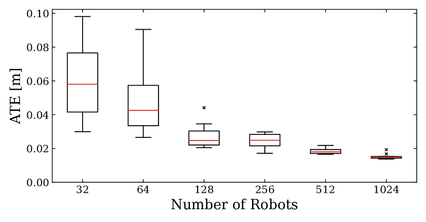
Instead, we present an experiment which demonstrates the scaling properties of Windowed GBP in a mode where the computation and communication work per robot is bounded. Figure 4 shows the average ATE of all robot pose estimates as the number of interacting robots in our arena is raised from 32 to 1024. The result is an average of over 10 different runs. Each robot measures nearby robots but is allowed to communicate with one other robot sampled based on Equation (76) per GBP iteration. Robot Web handles this extreme packing and scaling straightforwardly, and the ATE for all robots continues to decrease as robots are added due to the favourable high inter-connectedness of the whole graph, despite the minimal communication allowed. These results indicate the true potential of Robot Web methods towards very high numbers of simple interacting devices.

Figure 4: Extreme scaling: in a simulated environment, we increase the number of robots in the arena to over 1000, with each robot communicating with only one other per iteration of Windowed GBP, and therefore having a per-robot bounded computation and communication workload. The average ATE in all robots’ poses continues to decrease as we increase the number of robots. Each result is a summary of 10 runs with different random initialisation.

 

VI-D Operation with Outlier Measurements and Robust Factors

Figure 5: Robust factors enable remarkable resilience to a large fraction of outlier inter-robot sensor measurements, with ATE remaining low up to 70–80% of corrupt measurements to which a large amount of uniform noise is added. In a simulated environment, 50 robots are moving in an environment with 10 known landmarks for 100 poses each. Each result is a summary of 50 runs with different random initialisation.

 

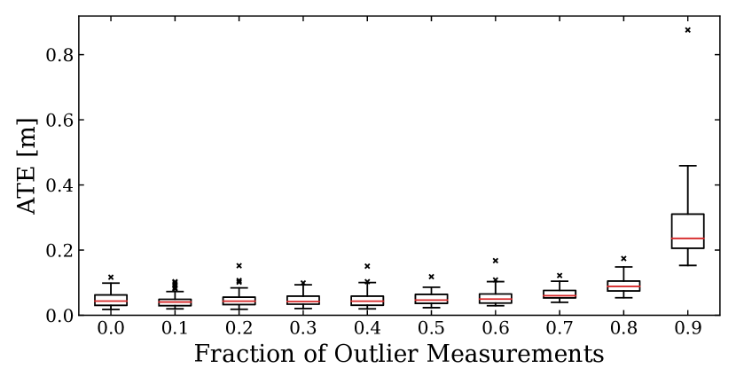
Here, we demonstrate the robustness of GBP using the method for handling robust factors from FutureMapping 2 [17] and the robust kernel from DCS [1]. 50 robots are used, each with a sliding window of 5. In Figure 5, we show what happens to the ATE when we increase the fraction of the range-bearing measurements containing the uniform noise. We see that a huge fraction of up to 80% of measurements can be completely corrupted but still handled by the robust measurement kernel with very little effect on the overall accuracy of the network. This again shows the advantage of the heavily inter-connected network which GBP allows us to efficiently and incrementally optimise in a distributed manner. In this network, each pose estimate is highly over-constrained, and this is what allows the robust kernel to weed out outlier measurements.

VI-E Operation with Unreliable Communication

Figure 6: Robot Web is highly robust to a high fraction of randomly dropped messages. In a simulated environment, 50 robots are moving in an environment with 10 known landmarks for 100 poses each. The result is a summary of 50 runs with different initialisation.

 

Figure 7: Analysis of the effect of varying the allowed communication range. ‘Inf’ means all robots are allowed to communicate with any other robot. While increasing the communication radius improves the performance, 30m onwards, the difference is negligible. In a simulated environment, 50 robots are moving in an environment with 10 known landmarks for 100 poses each. The result is a summary of 50 runs with different initialisation.

 

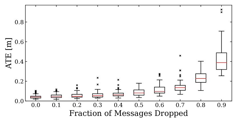
In multi-robot systems, another potential problem is the reliability of the communications. Often robots will communicate with best-effort, meaning messages can get lost in the network. Robustness against such data loss can be challenging; however, GBP is not significantly affected, as the message scheduling can be random. Here, we imagine that data transmission is quantised at the level of individual messages, as it might be with certain types of communication technology, and experiment to see the effect of the loss of a random fraction of messages between robots.

In Figure 6, we force the network to drop the messages randomly with a fixed probability which we gradually increase and investigate how that affects ATE. For example, if Robot $\alpha$ sends 3 rows of message $\{M_{1},M_{2},M_{3}\}$ to Robot $\beta$, the network may drop $M_{2}$, and Robot $\beta$ will only receive $\{M_{1},M_{3}\}$. In this experiment, we also see very advantageous properties for GBP, which retains a low ATE up to at least 50% message loss in this setting.

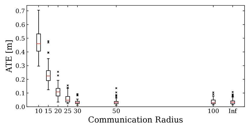
We further evaluate the effect of poor communication in terms of communication range. The communication radius of the robots was adjusted to range from 10m to 100m and an infinite radius. In line with previous experiments, each robot communicates with only one other robot per iteration. We disable the sliding window and perform a full pose update for this evaluation such that robots can exchange messages asynchronously on rendezvous.

As shown in Figure 7, reducing the communication range decreases the performance; however, beyond a radius of 25m, the performance improvements are minimal. In this configuration, there may be robots who never communicate with one another though they’ve made measurements of each other. As GBP has no synchronisation, such cases are simply ignored without the need for specific procedures.

VI-F Operation Under Poor Initialisation

Figure 8: Robot Web demonstrates its resilience to large initialisation errors. We add to the initial pose a noise sampled from a Gaussian with a standard deviation of ($n$ m, $n$ m, $n$ rad), where $n$ represents the noise level. Note that the graph is plotted on a logarithmic scale. In a simulated environment, 50 robots are moving in an environment with 10 known landmarks for 100 poses each. The result is a summary of 50 runs with different initialisation.

 

The initialisation is important for multi-robot localisation, especially for handling outlying measurements. However, good initialisation may not always be available in the real world. Here, we analyse the effect of increasing the noise on the initialisation and when the system breaks. We vary the $(\sigma_{x},\sigma_{y},\sigma_{\theta})$ from (0.1m, 0.1m, 0.1 rad) to (0.5m, 0.5m, 0.5 rad). The percentage of outlier range-bearing sensor measurements remains to be fixed at 10%.

We plot the graph on a logarithmic scale for clarity but notice that at noise level (0.5m, 0.5m, 0.5 rad), the value of the upper whisker is 3.51m whereas at (0.4m, 0.4m, 0.4 rad) it is 0.32m, clearly showing that the error explodes. Initialisation is critical for outlier rejection, and with a poor initialisation, good observations will have high energy and possibly lie in the outlier region of the robust kernel, making the optimisation problem challenging. While our approach demonstrates robustness against up to a large initialisation noise of (0.2m, 0.2m, 0.2 rad), improving the robustness to poor initialisation is an interesting direction for future works.

TABLE IV: A comparison of the different distributed solvers for solving multi-robot pose-graph optimisation. We report the initial cost, the solution of centralised Gauss-Newton (GN), and the cost and the number of iterations required for convergence for the different distributed solvers: distributed Block Gauss-Seidel (DGS) and distributed Block Jacobi Method from [13] and ours. Across all datasets, though distributed, our method and DGS obtains similar cost to the centralised GN.

Dataset	Initial Cost	Centralised GN	Block Gauss-Seidel		Block Jacobi Method		Ours
			#Iter	Cost	#Iter	Cost	#Iter	Cost
Sphere	$1.28863\times 10^{6}$	$8.43504\times 10^{2}$	723	$8.52218\times 10^{2}$	10000	$3.28738\times 10^{3}$	1240	$8.58949\times 10^{2}$
Torus	$1.88612\times 10^{6}$	$1.21137\times 10^{4}$	847	$1.23950\times 10^{4}$	6964	$1.25181\times 10^{5}$	1495	$1.22184\times 10^{4}$
Parking Garage	$8.36192\times 10^{3}$	$6.31262\times 10^{-1}$	117	$7.93764\times 10^{-1}$	5142	$8.16846\times 10^{3}$	1472	$6.94700\times 10^{-1}$
Cubicle	$2.53917\times 10^{6}$	$3.18310\times 10^{2}$	701	$3.38483\times 10^{2}$	9709	$2.20025\times 10^{3}$	244	$3.97225\times 10^{2}$
Rim	$4.06073\times 10^{7}$	$1.24992\times 10^{3}$	2355	$6.50345\times 10^{3}$	6142	$1.00088\times 10^{23}$	2932	$3.60934\times 10^{3}$
Grid	$7.21751\times 10^{7}$	$4.21596\times 10^{4}$	327	$4.24620\times 10^{4}$	5613	$4.96610\times 10^{4}$	1608	$4.23358\times 10^{4}$

VI-G Joining and Leaving the Robot Web

The Robot Web is fully dynamic because each robot does not need any information about the group as a whole, so robots can join or leave freely. When new robots are added, randomly into the arena, it is initialised at the centre of the arena and starts to participate in the Robot Web. It does not start to move until it believes that it has a good pose estimate. This decision is based on each robot monitoring the robust scaling of its factors, which is based on the Mahalanobis distance. Our implementation checks whether (a) the average scaling for all outgoing factors is $>0.95$, and (b) that there are at least 8 different observations. Until these criteria are met, the newly-added robots send empty messages on the inter-robot factors and therefore do not affect the already-initialised robots until they are confident enough to start moving and properly taking part in the web. A video demonstration of this in simulation is available here:
https://rmurai.co.uk/projects/RobotWeb#dynamic

VI-H Comparison against other solvers

While the focus of the paper is on distributed localisation using range-bearing sensor measurements, the fact that our method operates on an arbitrary factor graph enables the framework to work with different sensor modalities, for instance, inter-robot $\mathbf{SE}(3)$ transformation, often used in distributed pose-graph optimisation (PGO). Here, we solve the following problem:

$$\min_{\begin{subarray}{c}{{\mathbf{t}}}_{i}\in\mathbb{R}^{3},\\ {{\mathtt{R}}}_{i}\in\mathbf{SO}(3),\forall i\end{subarray}}\frac{1}{2}\sum_{\{i,j\}\in\varepsilon}\tau_{ij}\|{{\mathbf{t}}}_{j}-{{\mathbf{t}}}_{i}-{{\mathtt{R}}}_{i}{{\mathbf{t}}}^{z}_{i,j}\|^{2}_{2}+\kappa_{ij}\|{{\mathtt{R}}}_{j}-{{\mathtt{R}}}_{i}{{\mathtt{R}}}^{z}_{i,j}\|^{2}_{F}~{},~{}$$ (77)

where $\varepsilon$ is a set of all measurements, ${{\mathtt{R}}}_{i}$ is a rotation variable, ${{\mathbf{t}}}_{i}$ is a translation variable, ${{\mathtt{R}}}^{z}_{i,j}$ is the measured rotation from $i$ to $j$ and similarly ${{\mathbf{t}}}^{z}_{i,j}$ is the measured translation from $i$ to $j$. $\tau_{ij},\kappa_{ij}$ are the noise parameter computed from the dataset as done in [45, 50, 23].

The main complexities of PGO lie in how we handle poor initialisation. As the optimisation problem is non-convex, there exist many local minima. If we directly solve Equation (77), we will get stuck in a local minimum, even with small noise [10]. Following [13], we thus solve a relaxed, linear problem in two stages in a distributed manner. First, we solve the rotation problem:

$$\min_{{{\mathtt{R}}}_{i}\in\mathbf{SO}(3),\forall i}\frac{1}{2}\sum_{\{i,j\}\in\varepsilon}\kappa_{ij}\|{{\mathtt{R}}}_{j}-{{\mathtt{R}}}_{i}{{\mathtt{R}}}^{z}_{i,j}\|^{2}_{F}~{}.~{}$$ (78)

We solve the quadratic relaxation of this problem, by dropping the $\mathbf{SO}(3)$ constraint and then projecting the solution back to $\mathbf{SO}(3)$ via SVD.

We then solve for the full pose using a linear approximation of rotation perturbation:

$$\min_{{{\mathbf{t}}}_{i},\theta_{i}\in\mathbb{R}^{3},\forall i}\frac{1}{2}\sum_{\{i,j\}\in\varepsilon}\tau_{ij}\|{{\mathbf{t}}}_{j}-{{\mathbf{t}}}_{i}-{{\mathtt{R}}}_{i}\tilde{\operatorname{Exp}}(\theta_{i}){{\mathbf{t}}}^{z}_{i,j}\|^{2}_{2}$$

$$+\kappa_{ij}\|{{\mathtt{R}}}_{j}\tilde{\operatorname{Exp}}(\theta_{j})-{{\mathtt{R}}}_{i}\tilde{\operatorname{Exp}}(\theta_{i}){{\mathtt{R}}}^{z}_{i,j}\|_{F}^{2}~{},$$ (79)

where $\tilde{\operatorname{Exp}}(\theta)={{\mathtt{I}}}_{3}+{{\mathtt{S}}}(\theta)$, and ${{\mathtt{S}}}(\theta)$ is a skew symmetric matrix.

In [13], Equation (78), and (79) is solved using distributed Block Gauss-Seidel (DGS) or distributed Block Jacobi method. Here, we compare GBP and DGS for solving the two-stage PGO problem. We compare against DGS as it is used as an initialisation for other works [50, 49], and relaxation is simple to perform with the factor graph framework. In our evaluation, we report the initial and final cost and the number of iterations required to satisfy the termination condition. We evaluate the trajectories on pose-graph optimisation dataset [10]. Each trajectory is split into 50 segments to simulate a multi-robot pose-graph.

The setup of our evaluation favours the DGS. We count one iteration as a full DGS sweep, where the robots sequentially send the updated information to the next robots in a specific order. GBP on the contrary is robot-wise parallel and does not require coordinated updates. Hence, the communication pattern of GBP is closer to the distributed Block Jacobi method rather than DGS. Furthermore, we enable flagged initialisation for both DGS and distributed Block Jacobi method. For all methods, we terminate the iterations once the norm of the change in the rotation or the pose is below a specified threshold. Here, we use $10^{-2}$ as the threshold for both the rotation and the pose update, for all of our distributed solvers as recommended in [13]. Furthermore, for DGS and distributed Block Jacobi, we use the recommended relaxation parameter of 1.0 which we too found to work the best. We allow all the solvers to run for up to 10000 iterations.

As shown in Table IV, GBP performs comparable to DGS and obtains cost close to the centralised Gauss-Netwon solver, though the setup favours DGS, and DGS has distributed pose-graph specific heuristics such as flagged initialisation. Compared to the distributed Block Jacobi method which has a similar communication pattern as GBP, GBP performs significantly better, both in terms of final cost and the number of iterations. This result highlights the generality of GBP and makes GBP a promising alternative to the existing distributed solvers. Devising a fair and complete evaluation of different distributed solvers is an interesting direction for future work.

VII Demonstrations and Experiments in a Real-World

Figure 9: Image of a Turtlebot3 Burger used in the real robot experiment. It is fitted with AprilTag-labelled cubes, an Intel-Realsense D435i camera and Vicon markers. Vicon markers are only used to obtain the ground-truth trajectories, used for the evaluation. The depth image, laser scanner and IMU are not used in any of the experiments.

 

To provide concrete evidence of the effectiveness of our approach, we have evaluated the real robots running our system on onboard devices in a distributed manner.

VII-A Evaluation Setup

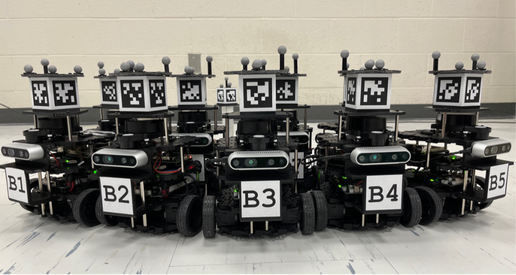
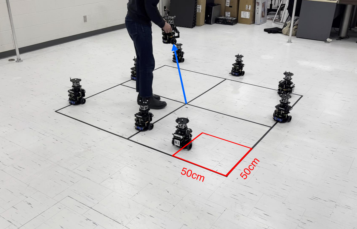
To evaluate our approach with real robots, we used nine TurtleBot3 Burgers as the robot platform. The robots (as shown in Figure 9) were equipped with a Raspberry Pi 3B+ computer with a Cortex-A53 64-bit 1.4GHz processor and 1GB of RAM as the onboard computer. In addition, each robot was fitted with an AprilTag-labeled cube – with the same tag on all sides – and an Intel-Realsense D435i camera. The RGB images captured by the camera and the data from the wheel encoder served as the sensory input. To simplify the setup, the depth image, IMU, and laser scanner were disabled, and for the odometry, only the wheel odometry was used. Each robot had knowledge of the size and location of the AprilTag [41], the camera position, and the calibration parameters. As we have many robots, factory calibration was used for the odometry and the camera. This is unideal as it adds systematic bias; however, our approach was still able to function effectively.

During the described experiment, the robots are instructed to follow a square trajectory. When the Robot Web system detects a drift in the robot’s position, a heuristic is used to correct the pose. For the drift of less than 5cm, proportional control is applied to bring the robot back onto the desired trajectory. Otherwise, the robot turns to face the next corner of the trajectory to correct the pose.

All computation, including GBP optimisation, pose correction, and inter-device communication via ROS2, runs on the onboard computer, highlighting the computational efficiency of our approach. We assume that the robots know the mapping between unique IDs and IP addresses in advance and that there is a shared/synchronised clock for all observations. When an AprilTag is detected, observation is transformed into a range-bearing measurement. We are unable to obtain relative transformation measurements – which include both translation and rotation – as the same AprilTag is used on all sides of the cube, so the orientation is ambiguous.

VII-B Implementation Details

We use ROS2 Foxy [39] for all the robots. The Publish-subscribe model as described in Section V-B is used for message passing. In ROS2 this entails simply subscribing to the topics (e.g. for robot 1, it will subscribe to robot_1/variable_msg, robot_1/factor_msg) and publishing to either the variable/factor of other robots along the inter-device factor.

GBP runs on its own thread, and the internal message passing runs as fast as possible. GBP is interleaved with the subscriber which receives the inter-device messages. For simplicity, a single coarse lock is used to avoid concurrency problems (adding inter-device messages to the internal factor graph); however, as all update operations of GBP are local, it is possible to use a finer lock. The publisher runs at 10Hz, publishing the outgoing messages. Best-effort delivery is used; hence, there is no delivery guarantee. We emphasise that the publishing and receiving of the messages are not synchronised, and robots receive messages at arbitrary timings (potentially out of order).

We set the sensor noise to be: $\sigma_{x}=0.01$m, $\sigma_{y}=0.01$m, and $\sigma_{\theta}=1^{\circ}$ for the prior; $\sigma_{x}=0.01$m, $\sigma_{y}=0.005$m, and $\sigma_{\theta}=1^{\circ}$ for the odometry; and $\sigma_{b}=0.01$m, and $\sigma_{\theta}=1^{\circ}$ for the range-bearing. All robots run GBP with a window size of 5. DSC [1] is used for the robust kernel with $\Phi=10$. The variable nodes are after any forward motion or a rotation, and in all the experiments, 75 poses per robot were added to the graph.

(a) No landmarks, no inter-device communication.

(b) No landmarks, with inter-device communication.

(c) With landmarks, no inter-device communication.

(d) With landmarks, with inter-device communication.

Figure 10: Nine real robots are moving in a square trajectory, and the motion captured by the Vicon system is plotted. It is clearly visible that using inter-device communication improves the localisation accuracy.

 

TABLE V: The table below shows the RMSE ATE of the real robot experiment. The RMSE ATE of the real robots is computed against the observations made by the Vicon motion capture system. The table summarises the impact of inter-device communication and the availability of landmarks on the RMSE ATE. We report the mean error and the standard deviation of the nine robots.

Communication	Landmark	$\mu\pm\sigma$ [m]
False	False	$0.162\pm 0.085$
True	False	$\mathbf{0.043\pm 0.020}$
False	True	$0.071\pm 0.020$
True	True	$\mathbf{0.028\pm 0.007}$

VII-C Multi-Robot Localisation Evaluation

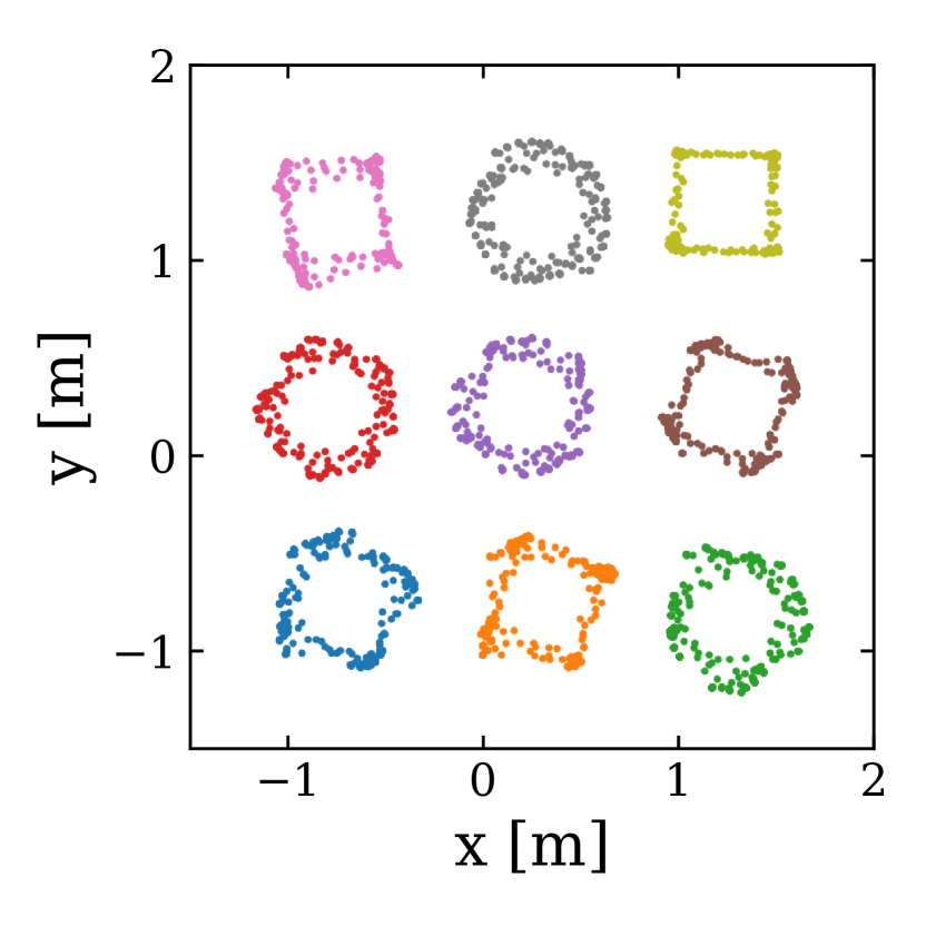
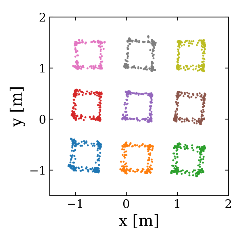
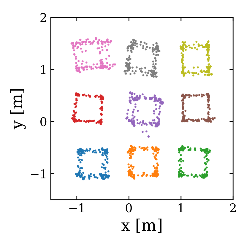
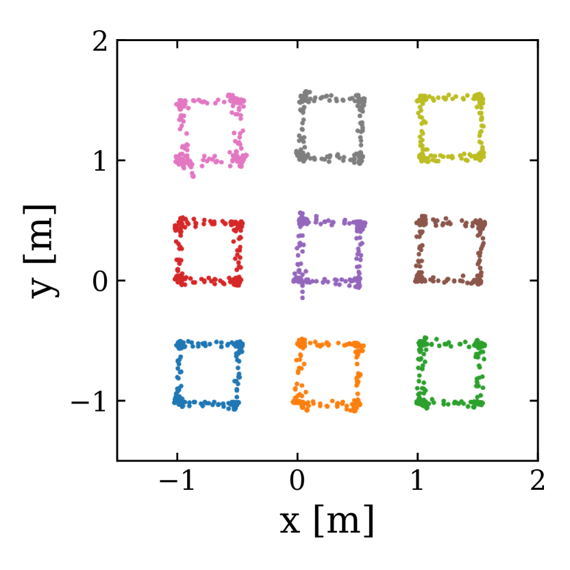
In this section, we evaluate the localisation accuracy of our approach. We evaluate under two different settings, with and without landmarks. Four landmarks are used, and their position is known to the robots in advance. Figure 10 shows the trajectory captured by the Vicon motion capture system. In all runs, robots are moving for 10 minutes. It is clear that Robot Web localises the robots well and allows them to operate for a long period without drifting.

The RMSE ATE of the real robots is computed against the observations made by the Vicon motion capture system. The result is summarised in Table V. As expected whether there are landmarks or not, using inter-device communication, i.e. using Robot Web, improves the localisation accuracy. The use of sparse landmarks is insufficient for good localisation without inter-device communication. This is clear both qualitatively by comparing (b) and (c) of Figure 10, and quantitatively in Table V by comparing: no landmarks, with inter-device communication; and with landmarks, no inter-device communication.

VII-D Relocalisation Demonstration

(a)

(b)

(c)

Figure 11: Here, nine robots are running Robot Web. Each robot starts on the vertices of the grid on the floor and moves in a square pattern (50cm x 50cm). In (a) during operation, one robot is removed from the system (e.g. for maintenance) and then added back with an incorrect pose. As a result, the robot fails to follow the square pattern, as shown in (b). However, using Robot Web, the robot is able to successfully relocalise, as shown in (c), and returns to following the square trajectory.

 

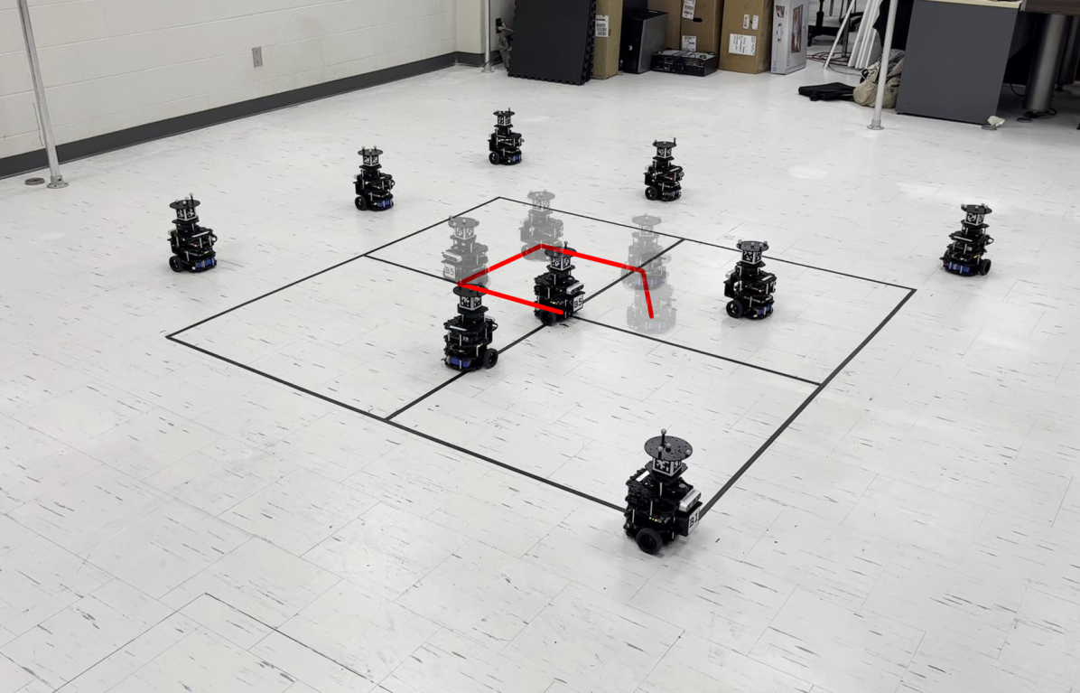
In a multi-robot system, there are many potential sources of failure for the robots. For instance, a robot might need to be stopped for maintenance due to a low battery, or it could be accidentally bumped out of position by a person. These types of external influences are often non-Gaussian, and if the system only accounts for Gaussian noise, it will not be able to accurately handle these unexpected events.

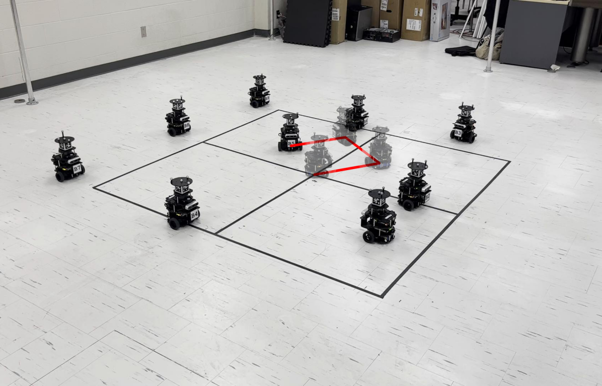
In Robot Web, while GBP assumes a Gaussian noise, robust factors allow the system to handle non-Gaussian noise as well. In Figure 11, we lift a moving robot and place it back in the wrong position. This disorients the robot, and it is unable to follow the square trajectory. However, after a few observations, the robot relocalises and returns to follow the square trajectory. During this relocalisation process, other robots are unaffected by the wrongly positioned robot as the robust factor heavily down weights its influence until the wrongly positioned robot is correctly localised. Due to the error between the position of the robot and its estimate, the measurements made of this robot by the others will have high residuals, and thus will be down-weighted by the robust kernel. A video of the relocalisation demo is available here:
https://rmurai.co.uk/projects/RobotWeb#reloc

VIII Ongoing Research Topics

We have demonstrated the essential operation of the Robot Web both in a simulation and in a real-world, truly distributed implementation on multiple robots. The properties of the method are extremely promising, and here we discuss some important research directions going forward.

VIII-A More General Parameterisation

Our current implementation makes several simplifying assumptions, but we believe that all of these are fairly straightforward to remove within the Robot Web framework with some further work.

• We currently assume that inter-robot measurement factors, stored by the robot with the sensor, always correspond to observations of the position of the centre of the second robot. This would already allow a practical implementation for 2D planar robots which each carry a single observable beacon above their centres. More realistically, each robot might have several or many observable features, and these will be located on any point on its structure. We can deal with this by adding additional internal variables to the second robot, connected to its main pose by ‘perfect’ factors, representing the positions of the observable features relative to its body, with positions that only need to be known to the second robot.

• Our current assumption that all robots have pose variables defined at the same rate and at corresponding times could be relaxed by measurement factors which connect to multiple variables at the receiving robot and interpolate the measurement between poses.

We might take the Robot Web idea even further to also apply inside a single robot’s modular body. The different parts, actuators and sensors that make up the robot might use Web interfaces between them to enable distributed joint estimation and very general modularity.

VIII-B Efficient Long-Term Operation

If we keep the full history of all pose variables for each robot, and all measurement factors, eventually the computation, storage and communication capacity of each robot would become overloaded. Of these, inter-robot communication is likely to be the main bottleneck. We showed one simple approach to dealing with this via time windowing, where poses older than a threshold are discarded, and this gives good performance when robots have bounded drift due to the presence of known beacons.

A more general approach to bounding the growth of the graph could be based on incremental abstraction [43], where past variables and factors are not deleted but grouped into more efficient blocks with minimal loss of accuracy. For instance, a set of well-estimated pose variables from the past could be grouped into an abstract trajectory segment, represented by far fewer variables. Factors could also be grouped. Achieving this incremental abstraction in a fully distributed way across multiple robots however will require substantial research.

IX Discussion and Conclusions

We have presented a method for distributed multi-robot localisation in the context of a larger ‘Robot Web’ vision for how heterogeneous groups of intelligent robots and devices of the future could cooperate and coordinate. This approach could be important at a time when many different companies and organisations are building spatially aware devices, and offers a distributed, inter-operable alternative to a single unified cloud maps solution.

As the performance and scale of many-robot systems may greatly improve due to work such as ours, it is important to consider potential ethical concerns. A robust, large-scale robot group or ‘swarm’ has many possible positive applications, such as the automation of farming or environmental surveillance via many low-cost devices, which could be much more efficient overall than a small number of large devices. However, there are possible ethical concerns with swarms of autonomous, weaponised drones

We believe that our paper overall could indicate a positive direction for the operation of distributed multi-robot systems via the specification that the Robot Web allows and demands of an open communication protocol. If the majority of the moving intelligent devices were to take part in such a system by publishing and reading localisation messages via this open protocol, it would be greatly to the advantage of any newly built devices to also take part, to exchange open messages, and to benefit from the system. This would mean that the whole system might work in a way similar to the World Wide Web, and some degree of global control would be possible via the interpretability of the protocol and perhaps more specific safety measures built into it. We believe that it is better for devices to be exchanging clearly interpretable geometric information than cryptic coded messages (as would emerge for instance in a possible distributed ‘graph neural network’ system for localisation, where the format of messages is learned rather than designed — and we should add here our view that a learned alternative to our method is also likely to be far less flexible and efficient).

These are ongoing issues to be debated as the technology advances, and we as authors believe that researchers should openly engage with these issues and play a part in designing the correct principles into the technology.

In the longer term future, the distributed coordination of intelligent moving systems is a key part of the concept of ‘intelligent matter’, where distribution and communication might be at the microscopic level to enable new classes of technology such as micromachines [26] which can self-organise in ways that might approach the capabilities of biological systems [29]. Recently, it has been shown that essentially the same computation framework that we have demonstrated in Robot Web using GBP can also be applied to multi-robot motion planning [44]. Efficient, robust distributed localisation will be one of the most important enabling layers of such systems.

References

- [1] P. Agarwal, G. D. Tipaldi, L. Spinello, C. Stachniss, and W. Burgard. Robust map optimization using dynamic covariance scaling. In Proceedings of the IEEE International Conference on Robotics and Automation (ICRA), 2012.
- [2] S. Agarwal, Mierle K., and Others. Ceres solver. http://ceres-solver.org.
- [3] Lars A. A. Andersson and Jonas Nygards. C-SAM : Multi-robot SLAM using square root information smoothing. In Proceedings of the IEEE International Conference on Robotics and Automation (ICRA), 2008.
- [4] R. Aragues, L. Carlone, G. Calafiore, and C. Sagues. Multi-agent localization from noisy relative pose measurements. In Proceedings of the IEEE International Conference on Robotics and Automation (ICRA), 2011.
- [5] Tim Bailey, Mitch Bryson, Hua Mu, John Vial, Lachlan McCalman, and Hugh Durrant-Whyte. Decentralised cooperative localisation for heterogeneous teams of mobile robots. In Proceedings of the IEEE International Conference on Robotics and Automation (ICRA), 2011.
- [6] Timothy D. Barfoot. State Estimation for Robotics. Cambridge University Press, 2017.
- [7] P. Barooah and J.P. Hespanha. Distributed estimation from relative measurements in sensor networks. In International Conference on Intelligent Sensing and Information Processing, 2005.
- [8] D. Bickson. Gaussian belief propagation: Theory and Application. PhD thesis, PhD thesis, The Hebrew University of Jerusalem, 2008.
- [9] Mauricio A. Caceres, Federico Penna, Henk Wymeersch, and Roberto Garello. Hybrid cooperative positioning based on distributed belief propagation. IEEE Journal on Selected Areas in Communications, 29(10):1948–1958, 2011.
- [10] Luca Carlone, Roberto Tron, Kostas Daniilidis, and Frank Dellaert. Initialization techniques for 3D SLAM: A survey on rotation estimation and its use in pose graph optimization. In Proceedings of the IEEE International Conference on Robotics and Automation (ICRA), 2015.
- [11] Josip Ćesić, Ivan Marković, Mario Bukal, and Ivan Petrović. Extended information filter on matrix Lie groups. Automatica, 82:226–234, 2017.
- [12] Yun Chang, Yulun Tian, Jonathan P. How, and Luca Carlone. Kimera-Multi: a system for distributed multi-robot metric-semantic simultaneous localization and mapping. In Proceedings of the IEEE International Conference on Robotics and Automation (ICRA), 2021.
- [13] S. Choudhary, L. Carlone, C. Nieto, J. Rogers, H. Christensen, and F. Dellaert. Distributed mapping with privacy and communication constraints: Lightweight algorithms and object-based models. International Journal of Robotics Research (IJRR), 36(12):1286–1311, 2017.
- [14] Titus Cieslewski, Siddharth Choudhary, and Davide Scaramuzza. Data-efficient decentralized visual SLAM. In Proceedings of the IEEE International Conference on Robotics and Automation (ICRA), 2018.
- [15] Alexander Cunningham, Vadim Indelman, and Frank Dellaert. DDF-SAM 2.0: Consistent distributed smoothing and mapping. In Proceedings of the IEEE International Conference on Robotics and Automation (ICRA), 2013.
- [16] Alexander Cunningham, Manohar Paluri, and Frank Dellaert. DDF-SAM: Fully distributed SLAM using constrained factor graphs. In Proceedings of the IEEE/RSJ Conference on Intelligent Robots and Systems (IROS), 2010.
- [17] A. J. Davison and J. Ortiz. FutureMapping 2: Gaussian Belief Propagation for Spatial AI. arXiv preprint arXiv:1910.14139, 2019.
- [18] F. Dellaert. Factor graphs and GTSAM. Technical Report GT-RIM-CP&R-2012-002, Georgia Institute of Technology, 2012.
- [19] F. Dellaert. Factor graphs: Exploiting structure in robotics. Annual Review of Control, Robotics, and Autonomous Systems, 4:141–166, 2021.
- [20] F. Dellaert and M. Kaess. Factor Graphs for Robot Perception. Foundations and Trends in Robotics, 6(1–2):1–139, 2017.
- [21] V. Delouille, R. Neelamani, and R. Baraniuk. Robust distributed estimation in sensor networks using the embedded polygons algorithm. In International Symposium on Information Processing in Sensor Networks, 2004.
- [22] R. M. Eustice, H. Singh, and J. J. Leonard. Exactly Sparse Delayed State Filters. In Proceedings of the IEEE International Conference on Robotics and Automation (ICRA), 2005.
- [23] Taosha Fan and Todd Murphey. Majorization minimization methods for distributed pose graph optimization with convergence guarantees. In Proceedings of the IEEE/RSJ Conference on Intelligent Robots and Systems (IROS), 2020.
- [24] Louis A. Hageman and David M. Young. Applied Iterative Methods. Academic Press, 1981.
- [25] Trevor Halsted, Olaoluwa Shorinwa, Javier Yu, and Mac Schwager. A survey of distributed optimization methods for multi-robot systems. ArXiv, abs/2103.12840, 2021.
- [26] T. Huang, H. Gu, and B. Nelson. Increasingly intelligent micromachines. Annual Review of Control, Robotics, and Autonomous Systems, 5:25.1–25.32, 2022.
- [27] Vadim Indelman, Erik Nelson, Nathan Michael, and Frank Dellaert. Multi-robot pose graph localization and data association from unknown initial relative poses via expectation maximization. In Proceedings of the IEEE International Conference on Robotics and Automation (ICRA), 2014.
- [28] M. Kaess, H. Johannsson, R. Roberts, V. Ila, J. Leonard, and F. Dellaert. iSAM2: Incremental Smoothing and Mapping Using the Bayes Tree. International Journal of Robotics Research (IJRR), 31(2):216–235, 2012.
- [29] C. Kaspar, B. J. Ravoo, W. G. van der Wiel, S. V. Wegner, and W. H. P. Pernice. The rise of intelligent matter. Nature, 594:345–355, 2021.
- [30] Been Kim, Michael Kaess, Luke Fletcher, John Leonard, Abraham Bachrach, Nicholas Roy, and Seth Teller. Multiple relative pose graphs for robust cooperative mapping. In Proceedings of the IEEE International Conference on Robotics and Automation (ICRA), 2010.
- [31] R. Kümmerle, G. Grisetti, H. Strasdat, K. Konolige, and W. Burgard. : A General Framework for Graph Optimization. In Proceedings of the IEEE International Conference on Robotics and Automation (ICRA), 2011.
- [32] P. Lajoie, B. Ramtoula, Y. Chang, L. Carlone, and G. Beltrame. DOOR-SLAM: Distributed, online, and outlier resilient SLAM for robotic teams. IEEE Robotics and Automation Letters, 5(2):1656–1663, 2020.
- [33] Pierre-Yves Lajoie, Benjamin Ramtoula, Fang Wu, and G. Beltrame. Towards collaborative simultaneous localization and mapping: a survey of the current research landscape. ArXiv, abs/2108.08325, 2022.
- [34] M. T. Lazaro, L. M. Paz, P. Pinies, J. A. Castellanos, and G. Grisetti. Multi-robot SLAM using condensed measurements. In Proceedings of the IEEE/RSJ Conference on Intelligent Robots and Systems (IROS), 2013.
- [35] Keith Y. Leung, Timothy D. Barfoot, and Hugh H. Liu. Decentralized cooperative SLAM for sparsely-communicating robot networks: A centralized-equivalent approach. Journal of Intelligent and Robotic Systems (JIRS), 66(3):3554–3561, 2012.
- [36] Keith Y. K. Leung, Timothy D. Barfoot, and Hugh H. T. Liu. Decentralized localization of sparsely-communicating robot networks: A centralized-equivalent approach. IEEE Transactions on Robotics (T-RO), 26(1):62–77, 2010.
- [37] Bin Li, Nan Wu, Hua Wang, Jingming Kuang, and Chengwen Xing. Gaussian message-based cooperative localization on factor graph in wireless sensor networks. In International Conference on Wireless Communications and Signal Processing, 2014.
- [38] Bin Li, Nan Wu, Hua Wang, Po-Hsuan Tseng, and Jingming Kuang. Gaussian message passing-based cooperative localization on factor graph in wireless networks. Signal Processing, 111:1–12, 2015.
- [39] Steven Macenski, Tully Foote, Brian Gerkey, Chris Lalancette, and William Woodall. Robot operating system 2: Design, architecture, and uses in the wild. Science Robotics, 7(66):eabm6074, 2022.
- [40] Kevin P Murphy, Yair Weiss, and Michael I Jordan. Loopy belief propagation for approximate inference: An empirical study. In Proceedings of the Fifteenth Conference on Uncertainty in Artificial Intelligence, pages 467–475. Morgan Kaufmann Publishers Inc., 1999.
- [41] Edwin Olson. AprilTag: A robust and flexible visual fiducial system. In Proceedings of the IEEE International Conference on Robotics and Automation (ICRA), 2011.
- [42] J. Ortiz, T. Evans, and A. J. Davison. A visual introduction to Gaussian Belief Propagation. arXiv preprint arXiv:2107.02308, 2021.
- [43] J. Ortiz, T. Evans, E. Sucar, and A. J. Davison. Incremental Abstraction in Distributed Probabilistic SLAM Graphs. Proceedings of the IEEE International Conference on Robotics and Automation (ICRA), 2022.
- [44] Aalok Patwardhan, Riku Murai, and Andrew J. Davison. Distributing collaborative multi-robot planning with gaussian belief propagation. IEEE Robotics and Automation Letters, 8(2):552–559, 2023.
- [45] D.M. Rosen, L. Carlone, A.S. Bandeira, and J.J. Leonard. SE-Sync: A certifiably correct algorithm for synchronization over the special Euclidean group. International Journal of Robotics Research (IJRR), 38(2–3):95–125, March 2019.
- [46] Jeremy Schiff, Erik B. Sudderth, and Ken Goldberg. Nonparametric belief propagation for distributed tracking of robot networks with noisy inter-distance measurements. In Proceedings of the IEEE/RSJ Conference on Intelligent Robots and Systems (IROS), 2009.
- [47] J. Solà, J. Deray, and D. Atchuthan. A micro Lie theory for state estimation in robotics. arXiv:1812.01537, 2018.
- [48] J. Sturm, N. Engelhard, F. Endres, W. Burgard, and D. Cremers. A Benchmark for the Evaluation of RGB-D SLAM Systems. In Proceedings of the IEEE/RSJ Conference on Intelligent Robots and Systems (IROS), 2012.
- [49] Y. Tian, K. Khosoussi, D. M. Rosen, and J. P. How. Distributed certifiably correct pose-graph optimization. IEEE Transactions on Robotics (T-RO), 37:2137–2156, 2021.
- [50] Yulun Tian, Alec Koppel, Amrit Singh Bedi, and Jonathan P. How. Asynchronous and parallel distributed pose graph optimization. IEEE Robotics and Automation Letters, 5(4):5819–5826, 2020.
- [51] Marco Todescato, Andrea Carron, Ruggero Carli, and L. Schenato. Distributed localization from relative noisy measurements: a robust gradient based approach. In European Control Conference (ECC), 2015.
- [52] Jiuqing Wan, Shaocong Bu, Jinsong Yu, and Liping Zhong. Distributed simultaneous localization and mapping for mobile robot networks via hybrid dynamic belief propagation. International Journal of Distributed Sensor Networks, 13(8):1–19, 2017.
- [53] Yair Weiss and William Freeman. Correctness of belief propagation in Gaussian graphical models of arbitrary topology. Advances in neural information processing systems, 12, 1999.
- [54] Henk Wymeersch, Jaime Lien, and Moe Z. Win. Cooperative localization in wireless networks. Proceedings of the IEEE, 97(2):427–450, 2009.
- [55] Yetong Zhang, Ming Hsiao, Jing Dong, Jakob Engel, and Frank Dellaert. MR-iSAM2: Incremental smoothing and mapping with multi-root Bayes tree for multi-robot SLAM. In Proceedings of the IEEE/RSJ Conference on Intelligent Robots and Systems (IROS), 2021.