The exact renormalization group and dimensional regularization

Abstract.

The exact renormalization group(ERG) is formulated implementing the decimation of degrees of freedom by means of a particular momentum integration measure. The definition of this measure involves a distribution that links this decimation process with the dimensional regularization technique employed in field theory calculations. Taking the dimension $d=4-\epsilon$, the one loop solutions to the ERG equations for the scalar field theory in this scheme are shown to coincide with the dimensionally regularized perturbative field theory calculation in the limit $\epsilon\to 0^{-}$, if a particular relation between the scale parameter $\mu$ and $\epsilon$ is employed. In general, it is shown that in this scheme the solutions to the ERG equations for the proper functions coincide when $\epsilon\to 0^{-}$ with the complete diagrammatic contributions appearing in field theory for these functions and this theory, provided that exact relations between $\mu$ and $\epsilon$ hold. In addition a non-perturbative approximation is considered. This approximation consists in a truncation of the ERG equations, which by means of a low momentum expansion leads to reasonable results.

1. Introduction

The Wilson renormalization group(WRG)[1] consists in the study of the evolution of systems under scale transformations. These scale transformations are implemented by means of the process of decimation. Decimation consists in integrating over certain degrees of freedom. A long distance effective theory is obtained by means of integrating out short distance degrees of freedom. The separation in short and long distance degrees of freedom involves the introduction of a length scale. This separation can be done in many different ways. In the original approach this was done by introducing a hard cut-off(HCO). The HCO method consists in including a step function in the integration measure for the modulus of the momenta. This procedure introduced non-local terms in coordinate space[2] and therefore a soft cut-off was proposed[1]. In the soft cut-off (SCO)version the step function employed in the HCO is replaced by a continuous function depending on a parameter which in a certain limit for this parameter tends to the step function. The implementation of this SCO into a effective field theory leads to the ERG equations. These equations are exact, they can be written for the proper functions of the theory, and take the form of one loop equations[4]. For the scalar $\phi$ field theory with symmetry under $\phi\to-\phi$, these equations give the derivative respect to the scale parameter of $n$-point proper functions in terms of other $j$-point functions, with $j=2,\cdots,n+2$.

On the other hand the field theoretic renormalization group(FTRG)[5][6] is related to making sense of the divergent contributions of Feynman diagrams in perturbation theory. In particular from the requirement that physical results should not depend on the subtraction procedure. This requirement gives information about the behavior of $n$-point functions under scaling of distances, which therefore provides a relation with the WRG. In both approaches particular techniques have been developed in order to study the renormalization group. In the FTRG dimensional regularization[7, 8](DR) and minimal subtraction play a prominent role. They provide a very practical calculation method and furthermore they are extremely useful when dealing with gauge theories, since they preserve gauge symmetry. DR is particular in the sense that the regularization is achieved by means of a analytic continuation in the number of dimensions. This is in contrast with other regularizations which directly modify the high momentum behavior of the propagator. Another difference between DR and other regularizations is that in DR it is necessary to introduce two parameters, $\epsilon$ the dimensionless deviation from the integer dimension $n$ considered and the energy scale $\mu$, which is used to give couplings the correct dimension in $d=n-\epsilon$ dimensions. In this work it will be shown that these two parameters should be related in order to re-obtain the field theory results as the solution to the ERG equations.

The purpose of this work is to give a version of the WRG which employs dimensional regularization. In order to achieve this, the decimation of degrees of freedom is linked with the dimensional regularization technique. The features and results of this work are summarized as follows,

• A integration measure over high momenta degrees of freedom is given, which links the HCO with dimensional regularization.

• The ERG equations for the proper functions of the scalar field theory with symmetry $\phi\to-\phi$ in four dimensions are considered in the above mentioned scheme.

• The $1$-loop perturbative solutions for the $2$-point and $4$-point proper functions to the ERG equations are obtained. They are shown to coincide with the dimensionally regularized field theoretic expressions, when $\epsilon\to 0^{-}$ and provided that a relation between the scale parameter $\mu$ and $\epsilon$ holds. Also the field renormalization function $\gamma$ is computed using the corresponding ERG equation at two loops.

• In general it is shown that the solutions to the ERG equations in this scheme for the proper functions, coincide with the complete diagrammatic contributions appearing in field theory for these functions when $\epsilon\to 0^{-}$. This is so, provided that for each $k$-point proper function a particular relation between the scale parameter $\mu$ and $\epsilon$ holds. This relation is exact and different for different $k$-point functions, but not universal.

• A non-perturbative approximation which consists in truncating the ERG equations is considered. Supplementing this truncation with a low momenta expansion gives to lowest order in the momenta reasonable results for the running of the $2$-point and 4-point couplings. In addition it is shown that higher orders in the momentum expansion can be calculated using the usual results for the integrals appearing in dimensionally regularized perturbative field theory.

The paper is organized as follows. Section 2 presents the integration measures and propagators of high and low momenta degrees of freedom. Section 3 gives the ERG equations for proper functions as they appear in ref. [4]. Section 4 deals with a loop expansion for the proper functions and computes the one loop expression for the $2$-point, the $4$-point functions and the field renormalization function $\gamma$ at two loops. Section 5 gives a diagrammatic non-perturbative proof that the solutions of the ERG equations coincides with the expression for these functions given in field theory. Section 6 presents a non-perturbative approximation for the $2$ and $4$ point proper functions, which consists in a truncation and a low momentum expansion. Finally, section 7 presents some concluding remarks and additional research motivated by this work.

2. Decimation and dimensional regularization

The theory to be considered is described by the following functional integral,

(2.1) $$Z[J]=\int\mathcal{D}\phi\,e^{\left(-\frac{1}{2}\int\phi\Delta^{-1}\phi-S_{I}[\phi]+\int J\phi\right)}$$

where the interaction term $S_{I}[\phi]$ is assumed to be given in terms of polynomials in the fields and its first derivatives, and such that,

$$S[\phi]=S[-\phi]$$

The propagator $\Delta$ appearing in (2.1) is taken to be,

(2.2) $$\Delta=\int\frac{d^{n}p}{(2\pi)^{n}}\Delta(p)\,e^{-ip\cdot(x-y)}\;\;,\Delta(p)=\frac{1}{p^{2}+m^{2}}$$

2.1. Integration measures over high and low momenta

The integration over momenta in $d$ dimensions is given by,

(2.3) $$d^{d}p=d\Omega_{d-1}dp\,p^{d-1}\;\;\;,d=n-\epsilon\;\;,$$

where $d\Omega_{d-1}$ is the integration measure over the $d-1$ dimensional unit sphere, for further use it is noted that,

$$S_{d-1}=\int d\Omega_{d-1}=(2\pi)^{d/2}\Gamma(d/2)$$

The integration over degrees of freedom is divided in two regions, low momenta and high momenta. In the hard cut-off version, this is done by using the following expression for the high momenta integration measure $d_{H}^{n}p$,

$$d_{H}^{n}p=d^{n}p\,\theta(\frac{p^{2}}{\mu^{2}}-1)$$

where $\mu$ is the mass scale mentioned above, and gives the separation between low momenta and high momenta. In this work this HCO is replaced by a soft cut-off version implemented by means of,

$$(\theta(x-x_{0}),\phi(x)) =\int_{x_{0}}^{\infty}dx\,\phi(x)$$

$$=\lim_{\epsilon\to 0}(\theta_{\epsilon}(x-x_{0}),\phi(x))=\lim_{\epsilon\to 0}\int_{x_{0}}^{\infty}dx\,x^{-\frac{\epsilon}{2}}\phi(x)$$

in this respect the limit $\epsilon\to 0$ is analogous to the hard cut-off limit mentioned in [9]. Decimation is implemented by integrating out in (2.1) the high momenta degrees of freedom.

2.2. The choice of the low $\Delta_{1}(p)$ and high $\Delta_{2}(p)$ momentum propagators

The momentum space propagator $\Delta(p)$ is divided into two parts, the low momenta propagator $\Delta_{1}$ and the high momenta propagator $\Delta_{2}$, i.e.,

$$\Delta(p)= \Delta_{1}(p,\mu)+\Delta_{2}(p,\mu)$$

where,

$$\Delta_{2}(p,\mu) =\frac{\theta_{\epsilon}(p^{2}/\mu^{2}-1)}{p^{2}+m^{2}}$$

The propagator will appear acting on functions of $p$, in expressions of the form,

$$I(q,\mu)=(\Delta_{2}(p,\mu),f(p,q))=\int d^{n}p\,\Delta_{2}(p,\mu)\,f(p,q)$$

where $F(p,q)$ is in general given by a product of momentum space complete propagators and $q$ generically denotes external momenta. In appendix A the r.h.s. of the previous equation is written in terms of a integration over $d=n-\epsilon$ dimensions and with no restriction on the modulus of the momenta. Using equation (7.1) in appendix A for,

$$f(p,q)=\frac{F(p.q)}{p^{2}+m^{2}}$$

leads to,

$$I(q,\mu) =\lim_{\epsilon\to 0}\frac{S_{n-1}}{S_{d-1}}\int d^{d}p\mu^{\epsilon}\left\{\frac{F(p.q)}{p^{2}+m^{2}}\right.$$

(2.4) $$\left.+\frac{\mu^{2}}{2p^{2}}\left[p\left(\frac{F^{(1,0)}(p,q)}{m^{2}+p^{2}}-\frac{2pF(p,q)}{\left(m^{2}+p^{2}\right)^{2}}\right)-2(\epsilon-1)\frac{F(p.q)}{p^{2}+m^{2}}\right]+\mathcal{O}(\frac{\mu^{4}}{p^{4}})\right\}$$

The action of $\mu\frac{\partial}{\partial\mu}\Delta_{2}(p)$ on functions will also be employed in what follows, using equation (7.2) in appendix A, leads to,

$$D(q,\mu) =(\mu\frac{\partial}{\partial\mu}\Delta_{2}(p,\mu),F(p,q))$$

$$=\epsilon I(q,\mu)+\lim_{\epsilon\to 0}\frac{S_{n-1}}{S_{d-1}}\int d^{d}p\mu^{\epsilon}\times$$

(2.5) $$\times\left\{\frac{\mu^{2}}{p^{2}}\left[p\left(\frac{F^{(1,0)}(p,q)}{m^{2}+p^{2}}-\frac{2pF(p,q)}{\left(m^{2}+p^{2}\right)^{2}}\right)-2(\epsilon-1)\frac{F(p.q)}{p^{2}+m^{2}}\right]+\mathcal{O}(\frac{\mu^{4}}{p^{4}})\right\}$$

3. The ERG equations for proper functions

The dimension in mass units of the momentum space dependent proper function $\Gamma_{k}$ after factoring a momentum-conservation delta function is,

(3.1) $$[\Gamma_{k}]=d-k\frac{(d-2)}{2}\overset{d=4-\epsilon}{=}4-\epsilon-k\left(1-\frac{\epsilon}{2}\right)=\left\{\begin{array}[]{cc}2&for\,k=2\\ \epsilon&for\,k=4\\ -2+2\epsilon&for\,k=6\\ -4+3\epsilon&for\,k=8\\ \vdots&\vdots\end{array}\right.$$

The ERG equations arise as a consequence of the requirement that the $k$ point correlators of the theory do not depend on the scale parameter $\mu$. As shown in [4], this requirement leads to the ERG equations satisfied by the proper functions $\Gamma_{k}$, which are given by,

(3.2) $$\left[\mu\frac{\partial}{\partial\mu}-p\cdot\frac{\partial}{\partial p}-k\frac{\gamma}{2}\right]\Gamma_{k}(p_{1},\cdots,p_{k}) =L_{k}(\{p\};\mu)$$

where,

$$L_{k}(p_{1},\cdots,p_{k};\mu) =\frac{\mu^{-\epsilon}}{2}\int\frac{d^{n}p}{(2\pi)^{n}}\left(\mu\frac{\partial}{\partial\mu}\Delta_{2}(p;\mu)\right)\int\frac{d^{n}q_{1}}{(2\pi)^{n}}\cdots\frac{d^{n}q_{l-1}}{(2\pi)^{n}}\times$$

$$\left[\sum_{p_{1}\cdots p_{l}}\bar{\Gamma}_{m_{1}+2}(p,-q_{1},p_{1}^{(1)},\cdots,p_{m_{1}}^{(1)})\mu^{-\epsilon}\Delta_{2}(q_{1})\right.$$

$$\times\bar{\Gamma}_{m_{2}+2}(q_{1},-q_{2},p_{1}^{(2)},\cdots,p_{m_{2}}^{(2)})\mu^{-\epsilon}\Delta_{2}(q_{2})\cdots$$

(3.3) $$\left.\bar{\Gamma}_{m_{l}+2}(q_{l-1},-p,p_{1}^{(l)},\cdots,p_{m_{l}}^{(l)})\right]$$

and,

$$m_{1}+m_{2}+\cdots+m_{l}=k$$

and the summation is over all possible ways of separating the $k$ momenta into $l$ sets, the set $j$ consisting of the $m_{j}$ momenta $p_{1}^{(j)},\cdots,p_{m_{j}}^{(j)}$.

For $k=2$ the equation (3.2) gives,

$$\mu\frac{\partial}{\partial\mu}\Gamma_{2}(p_{1};\mu) =\left(\gamma+p_{1}\cdot\frac{\partial}{\partial p_{1}}\right)\Gamma_{2}(p_{1};\mu)+$$

(3.4) $$+\frac{\mu^{-\epsilon}}{2}\int\frac{d^{n}p}{(2\pi)^{n}}\left(\mu\frac{\partial}{\partial\mu}\Delta_{2}(p;\mu)\right)\Gamma_{4}(p,-p,p_{1},-p_{1};\mu)$$

For $k=4$, (3.2) leads to,

$$\mu\frac{\partial}{\partial\mu}\Gamma_{4}(p_{1},p_{2},p_{3},p_{4};\mu) =\left(2\gamma+\sum_{i=1}^{3}p_{i}\cdot\frac{\partial}{\partial p_{i}}\right)\Gamma_{4}(p_{1},p_{2},p_{3},p_{4};\mu)$$

$$+\frac{\mu^{-\epsilon}}{2}\int\frac{d^{n}p}{(2\pi)^{n}} \left(\mu\frac{\partial}{\partial\mu}\Delta_{2}(p;\mu)\right)\Gamma_{6}(p,-p,p_{1},p_{2},p_{3},p_{4};\mu)$$

$$+\frac{\mu^{-\epsilon}}{2}\int\frac{d^{n}p}{(2\pi)^{n}}\frac{d^{n}p^{\prime}}{(2\pi)^{n}} \left(\mu\frac{\partial}{\partial\mu}\Delta_{2}(p;\mu)\Delta_{2}(p^{\prime};\mu)\right)$$

$$\times\left(\Gamma_{4}(p,-p^{\prime},p_{1},p_{2};\mu)\right. \,\Gamma_{4}(p^{\prime},-p,p_{3},p_{4};\mu)\delta^{(n)}(p-p^{\prime}+p_{1}+p_{2})$$

$$+\Gamma_{4}(p,-p^{\prime},p_{1},p_{3};\mu) \Gamma_{4}(p^{\prime},-p,p_{2},p_{4};\mu)\delta^{(n)}(p-p^{\prime}+p_{1}+p_{3})$$

(3.5) $$+\Gamma_{4}(p,-p^{\prime},p_{1},p_{4};\mu) \left.\Gamma_{4}(p^{\prime},-p,p_{2},p_{3};\mu)\delta^{(n)}(p-p^{\prime}+p_{1}+p_{4})\right)$$

the contributions involving momentum integrals to the right hand side of the previous equations can be associated to the graphs in figs. 3.1 and 3.2.

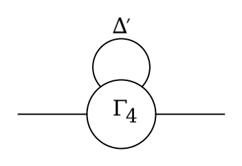
Figure 3.1. Graphical representation of $L_{2}$, in the figure $\Delta^{\prime}=\mu\frac{\partial}{\partial\mu}\Delta_{2}$.

Figure 3.2. Graphical representation of $L_{4}$. In this figure $\sum_{P}$ indicates summation over non-equivalent permutations of the external legs.

The initial conditions for a reference value $\mu_{0}$ of the mass scale, are taken to be,

$$\Gamma_{2}(p_{1};\mu_{0}) =-\left(p_{1}^{2}+m_{I}^{2}\right)\;\;\;,$$

$$\Gamma_{4}(p_{1},p_{2},p_{3};\mu_{0}) =-\lambda_{I}\;\;\;\lambda_{I}\ll 1,$$

(3.6) $$\Gamma_{2n}(\mu_{0}) =0\;\;\forall\,n>2$$

That is, the renormalization group flow is studied in the vicinity of a point which lies in the $(2-4)$ plane in the space of couplings, i.e. only $\Gamma_{2}$ and $\Gamma_{4}$ are assumed to be non-vanishing at the scale $\mu_{0}$. The solutions to (3.2) depend on the initial conditions (3.6). It is noted that $\lambda_{I}$ is dimension-full and $g_{I}=\lambda_{I}\mu^{-\epsilon}$ dimensionless.

It is important to state that fields will be rescaled so that the coupling $K$ corresponding to the kinetic term $Q$,

(3.7) $$Q=K\partial\phi\cdot\partial\phi\;\;,K=1$$

is equal to $1$. This entails a redefinition of the proper functions so that the effective action,

$$\Gamma[\phi]=\sum_{k=1}^{\infty}\frac{1}{k!}\int d^{n}x_{1}\cdots d^{n}x_{k}\,\Gamma_{k}(x_{1},\cdots,x_{k})\phi(x_{1})\cdots\phi(x_{k})$$

remains the same.

Condition (3.7) in terms of the two point function $G_{2}(p_{1},p_{2};\mu)$ is,

(3.8) $$\left.\frac{\partial^{2}}{\partial p_{1}^{2}}\Gamma_{2}(p_{1},p_{2};\mu)\right|_{p_{1}=0}=-1$$

The mass $m$ appearing in (LABEL:eq:delta2) and $m_{I}$ appearing in this initial condition differ by the factor $\sqrt{Z(\mu)}$ that accounts for the redefinition of the fields mentioned above, and is given by,

$$m^{2}=Z(\mu)m_{I}^{2}$$

Taking the second derivative of equation (3.4) respect to the external momenta $p_{1}$, evaluating at $p_{1}=0$ and using (3.8) , leads to a equation for $\gamma$,

(3.9) $$\gamma=-\frac{\mu^{-\epsilon}}{2}\left.\frac{\partial^{2}}{\partial p_{1}^{2}}\int\frac{d^{n}p}{(2\pi)^{n}}\left(\mu\frac{\partial}{\partial\mu}\Delta_{2}(p;\mu)\right)\Gamma_{4}(p,-p,p_{1},-p_{1};\mu)\right|_{p_{1}=0}$$

4. Loop expansion

A loop expansion for the proper functions consists in an expansion of the form,

(4.1) $$\Gamma_{2k}=\sum_{j}\gamma_{2k}^{(j)}$$

where $\gamma_{2k}^{(j)}$ is the contribution to $j$ loops. It is also convenient to define the partial sums,

$$\Gamma_{2k}^{(J)}=\sum_{j=1}^{J}\gamma_{2k}^{(j)}$$

which give the $2k$-point function up to $J$ loops.

It is important to bear in mind that in the r.h.s. of equations (3.4) and (3.5), the terms containing $\mu\frac{\partial}{\partial\mu}\Delta_{2}(p)$ are of one order higher in a loop expansion than the others. Thus the equations for the loop expansion coefficients are,

$$\mu\frac{\partial}{\partial\mu}\Gamma_{2}^{(j)}(p_{1};\mu) =\left(\gamma+p_{1}\cdot\frac{\partial}{\partial p_{1}}\right)\Gamma_{2}^{(j)}(p_{1};\mu)+$$

(4.2) $$\frac{1}{2}\int\frac{d^{n}p}{(2\pi)^{n}}\left(\mu\frac{\partial}{\partial\mu}\Delta_{2}(p;\mu)\right)\Gamma_{4}^{(j-1)}(p,-p,p_{1},-p_{1};\mu)$$

and,

$$\mu\frac{\partial}{\partial\mu}\Gamma_{4}^{(j)}(p_{1},p_{2},p_{3},p_{4};\mu)=\left(2\gamma+\sum_{i=1}^{3}p_{i}\cdot\frac{\partial}{\partial p_{i}}\right)\Gamma_{4}^{(j)}(p_{1},p_{2},p_{3},p_{4};\mu)$$

$$+\frac{1}{2}\int\frac{d^{n}p}{(2\pi)^{n}}\left(\mu\frac{\partial}{\partial\mu}\Delta_{2}(p;\mu)\right)\Gamma_{6}^{(j-1)}(p,-p,p_{1},p_{2},p_{3},p_{4};\mu)$$

$$+\frac{1}{2}\int\frac{d^{n}p}{(2\pi)^{d}}d^{n}p^{\prime}\left(\mu\frac{\partial}{\partial\mu}\Delta_{2}(p;\mu)\Delta_{2}(p^{\prime};\mu)\right)$$

$$\times\sum_{k,n/k+n=j-\text{1}}\left(\Gamma_{4}^{(k)}(p,-p^{\prime},p_{1},p_{2};\mu)\,\Gamma_{4}^{(n)}(p^{\prime},-p,p_{3},p_{4};\mu)\delta^{(d)}(p-p^{\prime}+p_{1}+p_{2})\right.$$

$$+\Gamma_{4}^{(k)}(p,-p^{\prime},p_{1},p_{3};\mu)\Gamma_{4}^{(n)}(p^{\prime},-p,p_{2},p_{4};\mu)\delta^{(d)}(p-p^{\prime}+p_{1}+p_{3})$$

(4.3) $$\left.+\Gamma_{4}^{(k)}(p,-p^{\prime},p_{1},p_{4};\mu)\Gamma_{4}^{(n)}(p^{\prime},-p,p_{2},p_{3};\mu)\delta^{(d)}(p-p^{\prime}+p_{1}+p_{4})\right)$$

Also,

$$\gamma^{(j)}=-\frac{\mu^{-\epsilon}}{2}\left.\frac{\partial^{2}}{\partial l_{1}^{2}}\int\frac{d^{n}l}{(2\pi)^{n}}\left(\mu\frac{\partial}{\partial\mu}\Delta_{2}(l;\mu)\right)\bar{g_{4}}^{(j-1)}(l,-l,l_{1},-l_{1};\mu)\right|_{l_{1}=0}$$

It is worth remarking that the first contributions to $\gamma$ start at two loops, because $\Gamma_{4}$ starts to depend on the external momenta at one loop.

4.1. k-point function at tree level

The equation for $\Gamma_{k}^{(0)},\;k\,$ even is,

$$\mu\frac{\partial}{\partial\mu}\Gamma_{k}^{(0)}(p_{1},\cdots,p_{k};\mu)=\left(\sum_{i=1}^{k}p_{i}\cdot\frac{\partial}{\partial p_{i}}\right)\Gamma_{k}^{(0)}(p_{1},\cdots,p_{k};\mu)$$

whose general solution is,

$$\Gamma_{k}^{(0)}(p_{1},\cdots,p_{k};\mu)=\Phi_{k}(\mu p_{1},\cdots,\mu p_{k})$$

with the initial condition,

$$\Gamma_{k}^{(0)}(p_{\text{1}},\cdots,p_{k};\mu_{0})=\begin{cases}\begin{array}[]{c}\Gamma_{2}^{(0)}(p_{1},p_{2};\mu_{0})=-\left(p_{1}^{2}+m_{I}^{2}\right)\;\;\;,\\ \Gamma_{4}^{(0)}(p_{1},p_{2},p_{3},p_{4};\mu_{0})=-\lambda_{I}\;\;\;\lambda_{I}\ll 1,\\ 0\end{array}&\begin{array}[]{c}k=2\\ k=4\\ k\geq 6\end{array}\end{cases}$$

leads to the particular solution,

$$\begin{array}[]{cc}\Gamma_{2}^{(0)}(p_{1},p_{2};\mu)=-\left(p_{1}^{2}\left(\frac{\mu}{\mu_{0}}\right)^{2}+m_{I}^{2}\right)&k=2\\ \Gamma_{4}^{(0)}(p_{1},p_{2},p_{3},p_{4};\mu)=-\lambda_{I}&k=4\\ \Gamma_{k}^{(0)}(p_{1},\cdots,p_{k};\mu)=0&k\geq 6\end{array}$$

where $m_{I}$ and $\lambda_{I}$ are constants that do not depend on $\mu$. Thus redefining the field by,

$$\tilde{\phi}=Z(\mu)^{-\frac{1}{2}}\phi\;\;,\;Z(\mu)=\left(\frac{\mu_{0}}{\mu}\right)^{2}\Rightarrow m_{I}^{2}=\left(\frac{\mu}{\mu_{0}}\right)^{2}m^{2}$$

which leads to a new k-point functions $\tilde{\Gamma}_{k}$, given by,

$$\tilde{\Gamma}_{k}=Z^{\frac{k}{2}}\Gamma_{k}$$

in particular for $n=2$, this gives,

$$\tilde{\Gamma}_{2}(p_{1})=Z\Gamma_{2}(p_{1})=-\left(p_{1}^{2}+m^{2}\right)$$

4.2. Two point function at one loop

To one loop order the above equation reduces to,

$$\left(\mu\frac{\partial}{\partial\mu}-p_{1}\cdot\frac{\partial}{\partial p_{1}}\right)\Gamma_{2}^{(1)}(p_{1};\mu)=\frac{1}{2}\int\frac{d^{n}p}{(2\pi)^{d}}\left(\mu\frac{\partial}{\partial\mu}\Delta_{2}(p)\right)\Gamma_{4}^{(0)}(p,-p,p_{1},-p_{1};\mu)$$

this is so because $\gamma=0$ at this loop order. Also it is noted that $\Gamma_{4}^{(0)}(p,-p,p_{1},-p_{1};\mu)=-\lambda_{I}$ independent of momenta, thus,

(4.4) $$\left(\mu\frac{\partial}{\partial\mu}-p_{1}\cdot\frac{\partial}{\partial p_{1}}\right)\Gamma_{2}^{(1)}(p_{1};\mu)=\lambda_{I}\mu^{-\epsilon}C(\mu)$$

where,

$$C(\mu) =-\frac{1}{2}\int\frac{d^{n}p}{(2\pi)^{d}}\mu\frac{\partial}{\partial\mu}\Delta_{2}(p)$$

employing equation (2.5) with $F(p,q)=1$, gives,

(4.5) $$C(\mu) =-\frac{1}{2}\frac{S_{n-1}}{S_{d-1}}\int\frac{d^{d}p}{(2\pi)^{d}}\mu^{\epsilon}\left\{\epsilon\frac{1}{p^{2}+m^{2}}+\frac{\mu^{2}}{p^{2}}.\left(\frac{\epsilon}{2}+1\right)\right.$$

(4.6) $$\times\left.\left(-2\frac{p^{2}}{(p^{2}+m^{2})^{2}}+2\frac{(1-\epsilon)}{p^{2}+m^{2}}\right)+\mathcal{O}(\epsilon)+\mathcal{O}\left(\frac{\mu^{4}}{p^{4}}\right)\right\}$$

it is noted that this expression is finite when $\epsilon\to 0$. In the first term inside the parenthesis this is so because this term is multiplied by $\epsilon$. For the second term this is so because the poles of the two terms inside the bracket cancel each other. The above expression can be explicitly evaluated using the usual dimensional regularization techniques leading to,

$$C(\mu)=\frac{S_{n-1}}{S_{d-1}}\frac{m^{2}}{(4\pi)^{2}}\left(\frac{\mu}{m}\right)^{\epsilon}\left(1-\frac{\mu^{2}}{m^{2}}+\mathcal{O}(\epsilon)+\mathcal{O}\left(\frac{\mu^{4}}{p^{4}}\right)\right)$$

This last expression is proportional to the $\gamma_{m}$ function defined by,

(4.7) $$\gamma_{m} =\frac{\mu}{m^{2}}\frac{\partial}{\partial\mu}\Gamma_{2}^{(1)}(0;\mu)=\frac{S_{n-1}}{S_{d-1}}\frac{1}{m^{2}}\lambda_{I}\mu^{-\epsilon}\frac{m^{2}}{(4\pi)^{2}}\left(\frac{\mu}{m}\right)^{\epsilon}\left(1-\frac{\mu^{2}}{m^{2}}\right)$$

(4.8) $$=\frac{S_{n-1}}{S_{d-1}}\frac{g_{I}}{(4\pi)^{2}}\left(\frac{\mu}{m}\right)^{\epsilon}\left(1-\frac{\mu^{2}}{m^{2}}\right)\overset{\epsilon\to 0}{=}\frac{g_{I}}{(4\pi)^{2}}\left(1-\frac{\mu^{2}}{m^{2}}\right)$$

it is important to note that the perturbative field theory beta function is given by the first term in the parenthesis above. The second term is a correction, which vanishes in the limit $\mu\to 0$, i.e. when the functional integration is done over all degrees of freedom.

Using the results in appendix B, the solution to (4.4) which reduces to the zero loop result when neglecting one-loop corrections, is,

$$\tilde{\Gamma}_{2}^{(1)}(p;\mu) =-p^{2}-m^{2}-\lambda_{I}\left[\int_{r_{0}}^{r}\frac{d\tilde{r}}{\tilde{r}}\right]_{r=\mu^{-1}}C(\mu)$$

$$=-p^{2}-m^{2}-\lambda_{I}\left[\log(r/r_{0})\right]_{r=\mu^{-1}}C(\mu)$$

$$=-p^{2}-m^{2}+\lambda_{I}\log(\mu/\mu_{0})C(\mu)$$

employing the expression in (4.5), the first term inside the parenthesis, leads to,

(4.9) $$\tilde{\Gamma}_{2}^{(1)}(p;\mu) =-p^{2}-m^{2}-\frac{\lambda_{I}}{2}\frac{S_{n-1}}{S_{d-1}}\log\left(\frac{\mu}{\mu_{0}}\right)\epsilon\int\frac{d^{d}p}{(2\pi)^{d}}\frac{1}{p^{2}+m^{2}}+\mathcal{O}(\epsilon)+\mathcal{O}\left(\mu^{2}\right)$$

At this point, it is quite natural to ask the following relevant question, how does the usual 1-loop perturbative expression for $\tilde{\Gamma}_{2}^{(1)}$ is obtained from this expression? The following relation between $\mu,\mu_{0}$ and $\epsilon$,

(4.10) $$\frac{S_{n-1}}{S_{d-1}}\log\left(\frac{\mu}{\mu_{0}}\right)\epsilon=1$$

gives an answer to the above question. Indeed, such a relation implies that,

• The coefficient of the third term in (4.9) is exactly the one appearing in the usual 1-loop perturbative expression for $\tilde{\Gamma}_{2}^{(1)}$.

• And,

  $$\frac{\mu}{\mu_{0}}=e^{\frac{1}{\epsilon}\frac{S_{n-1}}{S_{d-1}}}$$

  thus, for $\epsilon\to 0^{-}$ then $\mu\to 0$, which therefore make all the corrections $\mathcal{O}(\epsilon)$ and $\mathcal{O}\left(\mu^{2}\right)$ vanish in that limit.

It is worth noting that the limit $\mu\to 0$ corresponds to integrating over all degrees of freedom in the functional integral in equation (2.1), which is just the procedure employed to obtain the $1$-loop perturbative expression for $\Gamma_{2}^{(1)}$. It should be stressed that the above relation (4.10) is only required if the intention is to re-obtain the field theoretic result form the solution to ERG equation.

This contribution corresponds to the tadpole diagram shown below,

Figure 4.1. Tadpole diagram.

4.3. Four point function at one loop

Equation (4.3) for $j=0$ is,

$$\mu\frac{\partial}{\partial\mu}\Gamma_{4}^{(1)}(p_{1},\cdots,p_{4};\mu) =\left(2\gamma+\sum_{i=1}^{3}p_{i}\cdot\frac{\partial}{\partial p_{i}}\right)\Gamma_{4}^{(1)}(p_{1},\cdots,p_{4};\mu)$$

$$+\frac{(-\lambda_{I})^{2}\mu^{-\epsilon}}{2}\int\frac{d^{n}p}{(2\pi)^{n}}\frac{d^{n}p^{\prime}}{(2\pi)^{n}} \left(\Delta_{2}(p)\mu\frac{\partial}{\partial\mu}\Delta_{2}(p^{\prime})\right)$$

$$\sum_{P_{4}}\delta(p-p^{\prime}+p_{i_{1}}+p_{i_{2}})$$

where $\sum_{P_{4}}$ indicates a summation over all the $\frac{4!}{2!2!}=6$ different permutations of the form,

$$\left(\begin{array}[]{cccc}1&2&3&4\\ i_{1}&i_{2}&i_{3}&i_{4}\end{array}\right)$$

to this loop order $\gamma=0$ and using that,

$$\int d^{n}p\,\delta^{(n)}(p-p^{\prime})F(p)=F(p^{\prime})$$

leads to,

(4.11) $$\left(\mu\frac{\partial}{\partial\mu}-\sum_{i=1}^{3}p_{i}\cdot\frac{\partial}{\partial p_{i}}\right)\Gamma_{4}^{(1)}(p_{1},\cdots,p_{4};\mu)= \lambda_{I}^{2}\mu^{-\epsilon}A(p_{1},\cdots,p_{4})$$

where,

(4.12) $$A(p_{1},\cdots,p_{4})=B(p_{1}+p_{2})+B(p_{1}+p_{3})+B(p_{1}+p_{4})$$

and,

$$B(P) =\frac{1}{2}\int\frac{d^{n}p}{(2\pi)^{n}}\left(\mu\frac{\partial}{\partial\mu}\Delta_{2}(p)\Delta_{2}(p+P)\right)$$

$$=\frac{1}{2}\int\frac{d^{d}p}{(2\pi)^{d}}\left(\frac{\mu^{\epsilon}}{p^{2}+m^{2}}+\mathcal{O}\left(\frac{\mu^{2}}{p^{4}}\right)\right)\left(\frac{\epsilon}{(p+P)^{2}+m^{2}}+\mathcal{O}\left(\frac{\mu^{2}}{(p+P)^{4}}\right)\right)$$

$$=\frac{1}{2}\int\frac{d^{d}p}{(2\pi)^{d}}\frac{\epsilon\mu^{\epsilon}}{(p^{2}+m^{2})((p+P)^{2}+m^{2})}+\epsilon\times K+\mathcal{O}(\mu^{2})$$

where $K$ denotes a quantity which is finite when $\epsilon\to 0$. The solution to (4.11) which reduces to the zero loop result when neglecting one-loop corrections, is,

$$\Gamma_{4}^{(1)}(p_{1},\cdots,p_{4};\mu) =-\lambda_{I}-\lambda_{I}^{2}\mu^{-\epsilon}\left[\int_{r_{0}}^{r}\frac{d\tilde{r}}{\tilde{r}}A(\tilde{r}\mu\{p\})\right]_{r=\mu^{-1}}$$

in order to proceed the quantity $A(\tilde{r}\mu\{p\})$ is expanded as a power series in its argument. Only the first term in that expansion, i.e. $A(0)$ can contribute to $\Gamma_{4}^{(1)}$, this is so because the integrals appearing in $B(P)$ are multiplied by $\epsilon$, and only the first term in that power series can give something proportional to $\epsilon^{-1}$, the higher terms converge. Thus the relevant integral over $\tilde{r}$ is,

$$\int_{r_{0}}^{r}\frac{d\tilde{r}}{\tilde{r}}=\log(r/r_{0})$$

Thus,

$$\Gamma_{4}^{(1)}(p_{1},\cdots,p_{4};\mu) =-\lambda_{I}+\lambda_{I}^{2}\log(\mu/\mu_{0})\frac{\epsilon}{2}\frac{S_{n-1}}{S_{d-1}}\times$$

$$\int\frac{d^{d}p}{(2\pi)^{d}}\sum_{P}\frac{1}{(p^{2}+m^{2})((p+P)^{2}+m^{2})}+\epsilon\times K+\mathcal{O}(\mu^{2})$$

$$=-\lambda_{I}+\lambda_{I}^{2}\frac{1}{2}\sum_{P}\int\frac{d^{d}p}{(2\pi)^{d}}\frac{1}{(p^{2}+m^{2})((p+P)^{2}+m^{2})}+\epsilon\times K+\mathcal{O}(e^{-\frac{1}{2|\epsilon|}\frac{S_{n-1}}{S_{d-1}}})$$

where $\sum_{P}$ indicates a summation over $P=\{p_{1}+p_{2},p_{1}+p_{3},p_{1}+p_{4}\}$. As happens for the case of the two point function, relation (4.10) makes the term proportional to $\log(\mu/\mu_{0})\epsilon$ give the well known dimensionally regularized 1-loop expression for this correction and at the same time, makes the $\mathcal{O}(\mu^{2})$ corrections be negligible in the hard cut-off limit $\epsilon\to 0^{-}$. Thus assuming relation (4.10), then the dimensionally regularized 1-loop expression is re-obtained as the solution of the 1-loop ERG equation. This contribution corresponds to the fish diagram shown below,

Figure 4.2. Fish diagram.

4.4. $\gamma$ at two loops

The equation to be considered is,

$$\gamma^{(2)} =-\frac{\mu^{-\epsilon}}{2}\left.\frac{\partial^{2}}{\partial p_{1}^{2}}\int\frac{d^{d}p}{(2\pi)^{d}}\left(\mu\frac{\partial}{\partial\mu}\Delta_{2}(p;\mu)\right)\Gamma_{4}^{(1)}(p,-p,p_{1},-p_{1};\mu)\right|_{p_{1}=0}$$

$$=-\frac{\partial^{2}}{\partial p_{1}^{2}}\int\frac{d^{d}p}{(2\pi)^{d}}\left(\frac{\epsilon}{p^{2}+m^{2}}+\epsilon\times K^{\prime}+\mathcal{O}(\mu^{2})\right)\times$$

$$\;\;\left.\times\left(\lambda_{I}^{2}\log(\mu/\mu_{0})\frac{\epsilon}{2}\frac{S_{n-1}}{S_{d-1}}\int\frac{d^{d}p^{\prime}}{(2\pi)^{d}}\frac{1}{(p^{\prime 2}+m^{2})((p+p^{\prime}+p_{1})^{2}+m^{2})}+\epsilon\times K+\mathcal{O}(\mu^{2})\right)\right|_{p_{1}=0}$$

$$=-\frac{1}{2}\lambda_{I}^{2}\left.\frac{\partial^{2}}{\partial p_{1}^{2}}\int\frac{d^{d}p}{(2\pi)^{d}}\int\frac{d^{d}p^{\prime}}{(2\pi)^{d}}\left(\epsilon\frac{1}{p^{2}+m^{2}}\frac{1}{(p^{\prime 2}+m^{2})((p+p^{\prime}+p_{1})^{2}+m^{2})}\right)\right|_{p_{1}=0}$$

$$+\epsilon\times K"+\mathcal{O}(e^{-\frac{1}{2|\epsilon|}\frac{S_{n-1}}{S_{d-1}}})$$

where in the second equality it was used that the first term in (4.12) does not contribute to $\gamma$ because the corresponding integral does not depend on $p_{1}$, so that upon taking the derivative respect to this variable gives $0$. The other terms give the same contribution by pairs. In the third equality, relation (4.10) was employed. The first term in the r.h.s. of the last equality corresponds to the sunrise diagram, shown below,

Figure 4.3. Sunrise diagram.

thus it leads to the usual field theoretic two loop contribution to the $\gamma$ function associated with field renormalization. The $\epsilon$ in front of this expression retains only the coefficient of the simple pole when $\epsilon\to 0$ of the second derivative of this integral.

5. Solutions of dimensionally regularized ERG equations coincide with field theory calculation when $\epsilon\to 0^{-}$

The general form of the dimensionally regularized ERG equation is,

$$\left[\mu\frac{\partial}{\partial\mu}-p\cdot\frac{\partial}{\partial p}-\frac{n\gamma}{2}\right]\Gamma_{k}(\{p\};\mu)=L_{k}(\{p\};\mu)$$

where $\{p\}$ denotes the whole set of the $k$ external momenta $p_{1},p_{2},\cdots,p_{k}$ on which $\Gamma_{k}$ depends. The general solution to this equation, as shown in Appendix B, is given by,

$$\Gamma_{k}(\{p\},m,\mu)=\mu^{k\frac{\gamma}{2}}\left(\Phi(\mu\{p\},m)-\left[\int_{r_{0}}^{r}\frac{d\tilde{r}}{\tilde{r}^{1-k\frac{\gamma}{2}}}L_{k}(\tilde{r}\mu\{p\},m,\mu)\right]_{r=\mu^{-1}}\right)$$

where $\Phi(p\mu)$ is an arbitrary function of $p\mu$ to be fixed by boundary conditions. In this section it is shown that the above solution to the ERG equations coincides with the expression of the $n$-point proper function in terms of proper vertices linked by $\frac{1}{p^{2}+m^{2}}$ propagators when $\epsilon\to 0^{-}$.

First the case of the two point function $\Gamma_{2}$ is considered. The ERG equation in this case is,

(5.1) $$\left(\mu\frac{\partial}{\partial\mu}-\gamma-p_{1}\cdot\frac{\partial}{\partial p_{1}}\right)\Gamma_{2}(p_{1};\mu)=L_{2}(\,p_{1},\mu)$$

where,

$$L_{2}(\,p_{1},\mu)=\frac{\mu^{-\epsilon}}{2}\int\frac{d^{n}p}{(2\pi)^{n}}\left(\mu\frac{\partial}{\partial\mu}\Delta_{2}(p;\mu)\right)\Gamma_{4}(p,-p,p_{1},-p_{1};\mu)$$

using (2.5) leads to the following expression for $L_{2}$,

(5.2) $$L_{2}(\,p_{1},\mu)=\frac{1}{2}\frac{S_{n-1}}{S_{d-1}}\int\frac{d^{d}p}{(2\pi)^{.d}}\frac{\epsilon}{p^{2}+m^{2}}\Gamma_{4}(p,-p,p_{1},-p_{1};\mu)+\mathcal{O}\left(\frac{\mu^{2}}{p^{2}}\right)$$

the first term on the r.h.s. of the last equation is denoted by $L_{2}^{RD}(\,p_{1},\mu)$. In what follows the second terms of $\mathcal{O}\left(\mu^{2}/p^{2}\right)$ will be neglected, this procedure will be justified a posteriori. As shown in appendix B, the solution to (5.1) is,

(5.3) $$\Gamma_{2}(p_{1},m,\mu)=\mu^{\gamma}\left(\Phi(\mu p_{1},m)-\left[\int_{r_{0}}^{r}\frac{d\tilde{r}}{\tilde{r}^{1-\gamma}}L_{2}^{RD}(\tilde{r}\mu p_{1},m,\mu)\right]_{r=\mu^{-1}}\right)$$

in order to perform the integration appearing in the second term of the r.h.s. in the previous equation it is convenient to expand $L_{2}^{RD}(\tilde{r}\mu p_{1},m,\mu)$ in powers of the first argument, that is,

$$L_{2}^{RD}(\tilde{r}\mu p_{1},m,\mu)=\frac{1}{2}\frac{S_{n-1}}{S_{d-1}}\int\frac{d^{d}p}{(2\pi)^{.d}}\frac{\epsilon}{p^{2}+m^{2}}\sum_{j}\frac{(\tilde{r}^{2}\mu^{2}p_{1}^{2})^{j}}{2j!}\left[\frac{\partial^{(j)}}{\partial^{j}p_{1}^{2}}\Gamma_{4}(p,-p,p_{1},-p_{1};\mu)\right]{}_{p_{1}=0}$$

replacing this expression in (5.3), the integrals over $\tilde{r}$ are of the general form,

$$\mu^{2j+\gamma}\left[\int_{r_{0}}^{r}d\tilde{r}\tilde{r}^{\gamma-1+2j}\right]_{r=\mu^{-1}} =\mu^{2j+\gamma}\left(\frac{r^{\gamma+2j}-r_{o}^{2\gamma+j}}{\gamma+2j}\right)_{r=\mu^{-1}}$$

$$=\mu^{2j+\gamma}\left(\frac{\mu^{-\gamma-2j}-\mu_{o}^{-\gamma-2j}}{\gamma+2j}\right)$$

(5.4) $$=\left(\frac{1-(\mu/\mu_{0})^{\gamma+2j}}{\gamma+2j}\right)$$

At this point , it is important to note that, all the integrals over the momentum $p$ appearing in $L_{2}^{RD}$ are convergent for the terms in the summation with $j>1$. Thus, those terms do not contribute to $L_{2}^{RD}$ in the limit $\epsilon\to 0$. Noting the boundary condition (3.6), i.e. that for $\mu=\mu_{0}$, $\Gamma_{2}=-p_{1}^{2}-m_{I}^{2}$, leads to,

$$\Phi(\mu p_{1},m)=-\left(p_{1}\frac{\mu}{\mu_{0}}\right)^{2-\gamma}-\left(m\frac{\mu}{\mu_{0}}\right)^{2-\gamma}$$

Thus the term with $j=0$ gives the following contribution to $\Gamma_{2}$,

$$\Gamma_{2}(p_{1},m,\mu)=-p_{1}^{2}-m^{2}-\frac{\epsilon}{\gamma}\frac{S_{n-1}}{S_{d-1}}\left(1-(\mu/\mu_{0})^{\gamma}\right)\frac{1}{2}\int\frac{d^{d}p}{(2\pi)^{d}}\frac{1}{p^{2}+m^{2}}\Gamma_{4}(p,-p,0,0)$$

therefore if the following relation between $\epsilon$ and $\mu$ is imposed,

(5.5) $$1=-\frac{\epsilon}{\gamma}\frac{S_{n-1}}{S_{d-1}}\left(1-(\mu/\mu_{0})^{\gamma}\right)$$

then,

(5.6) $$\Gamma_{2}(p_{1}.m,\mu) =-p_{1}^{2}-m^{2}+\frac{1}{2}\int\frac{d^{d}p}{(2\pi)^{d}}\frac{1}{p^{2}+m^{2}}\Gamma_{4}(p,-p,0,0)$$

the r.h.s. of (5.6) is the dimensionally regularized expression for the proper two point function. Relation (5.5) is required in order to obtain the $2$-point function computed with dimensional regularization as a solution of the ERG equations. This relation links, the two parameters introduced by dimensional regularization, the dimensionless $\epsilon$ and the energy scale $\mu$. According to this relation, the limits $\mu\to 0$ and $\epsilon\to 0^{-}$ are equivalent. Relation (5.5) implies that,

$$\frac{\mu}{\mu_{0}}=\left(1+\frac{\gamma}{\epsilon}\frac{S_{d-1}}{S_{n-1}}\right)^{1/\gamma}\overset{\epsilon\to 0^{-}}{=}e^{-\frac{1}{|\epsilon|}\frac{S_{d-1}}{S_{n-1}}}$$

showing that the $\mathcal{O}(\mu^{2}/p^{2})$ appearing on the r.h.s. of (5.2) can be safely neglected in the limit $\epsilon\to 0^{-}$, as was done above. Inserting the loop expansion (4.1) for $\Gamma_{4}(p,-p,p_{1},-p_{1})$ leads to a loop expansion for $\Gamma_{2}(l_{1};\mu).$

The term with $j=1$ is the coefficient of the kinetic term. As stated in (3.8) this coefficient was fixed to $1$. Thus the contribution of this term is already taking into account in $\gamma$ given by (3.9).

Next, the general case of $\Gamma_{k}$ is considered. Appendix B gives the following general solution to the ERG equation for the $k$-point proper function,

(5.7) $$\Gamma_{k}(\{p\},m,\mu)=\mu^{k\frac{\gamma}{2}}\left(\Phi(\mu\{p\},m)-\left[\int_{r_{0}}^{r}\frac{d\tilde{r}}{\tilde{r}^{1-k\frac{\gamma}{2}}}L_{k}(\tilde{r}\mu\{p\},m,\mu)\right]_{r=\mu^{-1}}\right)$$

with $L_{k}(\{p\},m,\mu)$ given by,

$$L_{k}(p_{1},\cdots,p_{k},m,\mu) =\frac{\mu^{-\epsilon}}{2}\int\frac{d^{d}p}{(2\pi)^{d}}\left(\frac{\epsilon}{p^{2}+m^{2}}+\mathcal{O}(\mu^{2}/p^{2})\right)\left[\sum_{l=1}^{\infty}d^{d}q_{1}\cdots d^{d}q_{l-1}\right.$$

$$\times\sum_{m_{1}\cdots m_{l}}\bar{\Gamma}_{m_{1}+2}(p,-q_{1},p_{1}^{(1)},\cdots,p_{m_{1}}^{(1)})\mu^{-\epsilon}\left(\frac{\mu^{\epsilon}}{q_{1}^{2}+m^{2}}+\mathcal{O}(\mu^{2}/q_{1}^{2})\right)$$

$$\times\bar{\Gamma}_{m_{2}+2}(q_{1},-q_{2},p_{1}^{(2)},\cdots,p_{2}^{(2)})\mu^{-\epsilon}\left(\frac{\mu^{\epsilon}}{q_{2}^{2}+m^{2}}+\mathcal{O}(\mu^{2}/q_{2}^{2})\right)$$

(5.8) $$\left.\times\cdots\bar{\Gamma}_{m_{l}+2}(q_{k-1},-p,p_{1}^{(l)},\cdots,p_{m_{l}}^{(l)})\right]$$

where,

$$m_{1}+m_{2}+\cdots+m_{l}=k$$

and the summation is over all possible ways of separating the $k$ momenta into $l$ sets, the set $j$ consisting of the $m_{j}$ momenta $p_{1}^{(j)},\cdots,p_{m_{j}}^{(j)}$. In (5.8), equations (2.4) and (2.5) were employed to write $\Delta_{2}$ and $\mu\frac{\partial}{\partial\mu}\Delta_{2}$ respectively. Denoting by $L_{k}^{RD}(p_{1},\cdots,p_{k},m,\mu)$ the contribution to $L_{k}$ obtained by neglecting the $\mathcal{O}\left(\mu^{2}/p^{2}\right)$ terms , leads to,

$$\bar{\Gamma}_{k}(\{p\};\mu) =\mu^{\frac{k}{2}\gamma}\left(\Phi(\{p\}\mu,m)-\int_{\mu_{0}}^{\mu}d\tilde{r}\,\tilde{r}^{-1+\frac{k}{2}\gamma}L_{k}^{RD}(\tilde{r}\mu\{p\},m,\mu)\right)$$

proceeding as in the case of the $2$-point function, that is expanding $L_{k}^{RD}(\tilde{r}\mu\{p\},m,\mu)$ as a power series in the first argument, the integrals over $\tilde{r}$ are the same as in (5.4). For $k>2$ only the first term of the power series mentioned above contributes in the limit $\epsilon\to 0$. Extracting the factor $\frac{S_{n-1}}{S_{d-1}}\epsilon$ in front of $L_{k}(p)$ and using the relation,

(5.9) $$\frac{1}{\epsilon}=-\frac{2}{k\gamma}\frac{S_{n-1}}{S_{d-1}}\left(1-(\mu/\mu_{0})^{\frac{k}{2}\gamma}\right)$$

gives,

(5.10) $$\Gamma_{k}(\{p\},m,\mu)=\mu^{\frac{k}{2}\gamma}\left(\Phi(\{p\}\mu,m\})-\tilde{\Gamma}_{k}^{RD}(\{p\},m,\mu)\right)$$

where $\tilde{\Gamma}_{k}^{RD}(p)$ is given by,

$$\tilde{\Gamma}_{k}^{RD}(\{p\},m,\mu)= \frac{\mu^{-\epsilon}}{2}\int\frac{d^{d}p}{(2\pi)^{d}}\frac{\epsilon}{p^{2}+m^{2}}\left[\sum_{l=1}^{\infty}d^{d}p_{1}\cdots d^{d}p_{l}\right.$$

$$\times\sum_{m_{1}\cdots m_{l}}\bar{\Gamma}_{m_{1}+2}(p,-p_{1},p_{1}^{(1)},\cdots,p_{m_{1}}^{(1)})\frac{1}{p_{1}^{2}+m^{2}}$$

$$\times\bar{\Gamma}_{m_{2}+2}(p_{1},-p_{2},p_{1}^{(2)},\cdots,p_{2}^{(2)})\frac{1}{p_{2}^{2}+m^{2}}$$

(5.11) $$\left.\times\cdots\bar{\Gamma}_{m_{l}+2}(p_{k-1},-p,p_{1}^{(l)},\cdots,p_{m_{l}}^{(l)})\right]$$

as for the case of $L_{2}$, the contribution of the additional $\mathcal{O}\left(\mu^{2}/p^{2}\right)$ appearing in (5.8) can be safely neglected in the limit $\epsilon\to 0^{-},$ if relation (5.9) is imposed. In appendix C it is shown that expression (5.10) coincides with the one obtained in field theory.

It is important to emphasize that the fact that the relation,

(5.12) $$\frac{1}{\epsilon}=-\frac{S_{n-1}}{S_{d-1}}\frac{2}{k\gamma}\left(1-(\mu/\mu_{0})^{\frac{k}{2}\gamma}\right)$$

is required to obtain coincidence of the solutions of the ERG equations for the $k$-point proper function with the field theory contributions, is a non-perturbative exact result. This is so since in this section no perturbative approximation has been employed. On the other hand this relation is not universal, indeed all critical exponents are given in terms of beta functions, which do not involve the integrals over $r$ which give rise to relation (5.12). In addition if $\epsilon$ is changed by a factor, then this factor does not affect the critical exponents, but it will change the relation (5.12), also if the normalization of the kinetic term is changed then, as shown above, $\gamma$ changes and this affects the form of relation (5.12).

6. Non-perturbative approximation

The approximation consists in first truncating the ERG to a given order. The truncation where $\Gamma_{n}=0\;,\forall n>4$ is considered. This truncation is justified since $\Gamma_{n}$ for $n>4$ correspond to irrelevant operators whose couplings will vanish when going to the infrared. Then the truncated equations for $\Gamma_{2}$ and $\Gamma_{4}$ are (3.4) and (3.5), where in the last one, due to the truncation, the first term on the r.h.s. does not appear, i.e. the truncated ERG equations are,

$$\mu\frac{\partial}{\partial\mu}\Gamma_{2}(p_{1};\mu) =\left(\gamma+p_{1}\cdot\frac{\partial}{\partial p_{1}}\right)\Gamma_{2}(p_{1};\mu)$$

$$+\frac{\mu^{-\epsilon}}{2}\int\frac{d^{d}p}{(2\pi)^{d}}\left(\mu\frac{\partial}{\partial\mu}\Delta_{2}(p;\mu)\right)\Gamma_{4}(p,-p,p_{1},-p_{1};\mu)$$

$$\mu\frac{\partial}{\partial\mu}\Gamma_{4}(p_{1},p_{2},p_{3},p_{4};\mu) =\left(2\gamma+\sum_{i=1}^{4}p_{i}\cdot\frac{\partial}{\partial p_{i}}\right)\Gamma_{4}(p_{1},p_{2},p_{3},p_{4};\mu)$$

$$+\frac{\mu^{-2\epsilon}}{2}\int\frac{d^{d}p}{(2\pi)^{d}}d^{d}p^{\prime}\left(\Delta_{2}(p;\mu)\mu\frac{\partial}{\partial\mu}\Delta_{2}(p^{\prime};\mu)\right)$$

$$\times\left(\Gamma_{4}(p,-p^{\prime},p_{1},p_{2};\mu)\Gamma_{4}(p^{\prime},-p,p_{3},p_{4};\mu)\delta^{(d)}(p-p^{\prime}+p_{1}+p_{2})\right.$$

$$+\Gamma_{4}(p,-p^{\prime},p_{1},p_{3};\mu)\Gamma_{4}(p^{\prime},-p,p_{2},p_{4};\mu)\delta^{(d)}(p-p^{\prime}+p_{1}+p_{3})$$

(6.1) $$\left.+\Gamma_{4}(p,-p^{\prime},p_{1},p_{4};\mu)\Gamma_{4}(p^{\prime},-p,p_{2},p_{3};\mu)\delta^{(d)}(p-p^{\prime}+p_{1}+p_{4})\right)$$

as in section 5 , the derivative respect to the external momenta in these equations can be written as,

$$\sum_{i=1}^{k}p_{i}\cdot\frac{\partial}{\partial p_{i}}\Gamma_{k}(p_{1},\cdots,p_{k})=\left.\rho\frac{\partial}{\partial\rho}\Gamma_{k}(\rho p_{1},\cdots,\rho p_{k})\right|_{\rho=1}$$

in addition the following low momenta expansion is proposed,

$$\Gamma_{k}(\rho p_{1},\cdots,\rho p_{k})=\sum_{j=0}^{\infty}\rho^{j}\Gamma_{k}^{(j)}(p_{1},\cdots,p_{k})$$

putting $\rho=0$ on both sides of this equation implies that $\Gamma_{k}^{(0)}$ does not depend on the momenta, in general the coefficient $\Gamma_{k}^{(j)}(p_{1},\cdots,p_{k})$, will be a polynomial of degree $j$ in the momenta with all Lorentz indices contracted. In addition the zeroth order $\gamma$ function given by (3.9) vanishes, because $\Gamma_{4}^{(0)}$ does not depend on the external momenta. Thus the truncated equation up to order $\mathcal{O}(\rho^{0})$ is,

$$\mu\frac{\partial}{\partial\mu}\Gamma_{4}^{(0)}(\mu) =\frac{3}{2}\left(\Gamma_{4}^{(0)2}(\mu)\mu^{-2\epsilon}\right)\frac{1}{2}\int\frac{d^{d}p}{(2\pi)^{d}}\left(\Delta_{2}(p;\mu)\mu\frac{\partial}{\partial\mu}\Delta_{2}(p;\mu)\right)$$

$$=\frac{3}{4}\left(\Gamma_{4}^{(0)2}(\mu)\mu^{-2\epsilon}\right)\epsilon\int\frac{d^{d}p}{(2\pi)^{d}}\left(\frac{\mu^{2\epsilon}}{(p^{2}+\Gamma_{2}^{(0)}(\mu)^{2})^{2}}\right)$$

$$=\frac{3}{4}\Gamma_{4}^{(0)2}(\mu)\frac{\Gamma_{2}^{(0)}(\mu)^{-\epsilon}}{(4\pi)^{2-\frac{\epsilon}{2}}}\epsilon\Gamma(\frac{\epsilon}{2})\overset{\epsilon\to 0}{=}\frac{3}{2(4\pi)^{2}}\Gamma_{4}^{(0)2}(\mu)$$

the previous equation gives the beta function for the coupling $\Gamma_{4}^{(0)}(\mu)$. The solution to this equation is,

$$\Gamma_{4}^{(0)}(\mu)=-\frac{\lambda_{I}}{1-\lambda_{I}\frac{3}{2(4\pi)^{2}}\log\left(\frac{\mu}{\mu_{0}}\right)}$$

, which satisfies the boundary condition (3.6). This shows that the effective coupling $\lambda=-\Gamma_{4}^{(0)}(\mu)$ as a function of $\mu$ for $\mu<\mu_{0}$, is smaller than its initial value $\lambda_{I}$. Even if the initial coupling $\lambda_{I}$ is $\lambda_{I}\gg 1$, the effective coupling saturates at a value $\lambda_{s}=-\frac{(4\pi)^{2}}{3\log\left(\frac{\mu}{\mu_{0}}\right)}$ . Replacing this result in the equation for $\Gamma_{2}^{(0)}(\mu)$ leads to,

$$\mu\frac{\partial}{\partial\mu}\Gamma_{2}^{(0)}(\mu) =-\frac{\mu^{-\epsilon}}{2}\frac{\lambda_{I}}{1-\lambda_{I}\frac{3}{2(4\pi)^{2}}\log\left(\frac{\mu}{\mu_{0}}\right)}\int\frac{d^{d}p}{(2\pi)^{d}}\left(\mu\frac{\partial}{\partial\mu}\Delta_{2}(p;\mu)\right)$$

$$=-\frac{\mu^{-\epsilon}}{2}\frac{\lambda_{I}}{1-\lambda_{I}\frac{3}{2(4\pi)^{2}}\log\left(\frac{\mu}{\mu_{0}}\right)}\mu^{\epsilon}\int\frac{d^{d}p}{(2\pi)^{d}}\left[\frac{\epsilon}{p^{2}+\Gamma_{2}^{(0)}(\mu)}\right.$$

$$\left.-(2+\epsilon)\left(\frac{\mu^{2}}{(p^{2}+\Gamma_{2}^{(0)}(\mu))^{2}}-\frac{\mu^{2}}{p^{2}(p^{2}+\Gamma_{2}^{(0)}(\mu))}\right)\right]$$

$$=-\frac{\lambda_{I}}{1-\lambda_{I}\frac{3}{2(4\pi)^{2}}\log\left(\frac{\mu}{\mu_{0}}\right)}\left(\frac{\Gamma_{2}^{(0)}(\mu)^{(1-\epsilon/2)}}{(4\pi)^{2-\frac{\epsilon}{2}}}\left(1+(2+\epsilon)\frac{\mu^{2}}{\Gamma_{2}^{(0)}(\mu)^{1+\epsilon/2}}\right)+\mathcal{O}(\epsilon)\right)$$

$$\overset{\epsilon\to 0}{=}\frac{\lambda_{I}}{1-\lambda_{I}\frac{3}{2(4\pi)^{2}}\log\left(\frac{\mu}{\mu_{0}}\right)}\frac{\Gamma_{2}^{(0)}(\mu)}{(4\pi)^{2}}\left(1+2\frac{\mu^{2}}{\Gamma_{2}^{(0)}(\mu)}\right)=\lambda\frac{\Gamma_{2}^{(0)}(\mu)}{(4\pi)^{2}}\left(1+2\frac{\mu^{2}}{\Gamma_{2}^{(0)}(\mu)}\right)$$

the solution to this equation with the initial condition,

$$\Gamma_{2}^{(0)}(\mu_{0})=-m_{I}^{2}$$

is,

$$\Gamma_{2}^{(0)}(\mu)=\frac{4}{3}e^{\frac{64\pi^{2}}{3\lambda}}\text{$\mu_{0}^{2}$}E_{\frac{1}{3}}\left(\frac{64\pi^{2}}{3\lambda}-2\log\left(\frac{\mu}{\text{$\mu_{0}$}}\right)\right)-\frac{32\sqrt[3]{2}\pi^{4/3}e^{\frac{64\pi^{2}}{3\lambda}}\text{$\mu_{0}^{2}$}E_{\frac{1}{3}}\left(\frac{64\pi^{2}}{3\lambda}\right)+24\sqrt[3]{2}\pi^{4/3}m_{I}^{2}}{3\left(32\pi^{2}-3\lambda\log\left(\frac{\mu}{\text{$\mu_{0}$}}\right)\right)^{2/3}}$$

where $E_{\frac{1}{3}}$ denotes the exponential integral function with index $1/3.$ It is noted that the effective squared mass $m^{2}=-\Gamma_{2}^{(0)}(\mu)$ for fixed $\mu<\mu_{0}$, decreases as a function of $\lambda_{I}$. The effective coupling $\lambda$ and mass squared $\frac{m^{2}}{\mu_{0}^{2}}$ are plotted as a function of $\frac{\mu}{\mu_{0}}$ in the range $0.001$ to $0.3$,

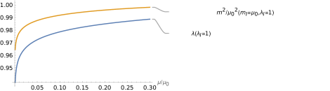
Figure 6.1. The effective coupling and mass squared for initial values $\lambda_{I}=1,\,m_{I}^{2}=\mu_{0}^{2}$, are plotted as a function of $\frac{\mu}{\mu_{0}}$ in the range $0.001$ to 0.3

the above shows that these results are consistent with assuming a low momenta dependence of these quantities.

Higher order terms in the low momentum expansion can be computed. For example for the case of $\Gamma_{4}$ the momentum integrals that appear are of the form,

$$\int\frac{d^{d}p}{(2\pi)^{d}}\frac{p^{\mu_{1}}\cdots p^{\mu_{n}}}{(p^{2}+m_{I}^{2})((p+P)^{2}+m_{I}^{2})}$$

these integrals can be computed in the usual way, i.e. using Feynman trick,

$$\frac{1}{AB}=\int_{0}^{1}\frac{dx}{[Ax+B(1-x)]^{2}}$$

and the result for the momentum integrals of the form,

$$F_{n}^{\mu_{1}\cdots\mu_{n}}=\int\frac{d^{d}p}{(2\pi)^{d}}\,\frac{p^{\mu_{1}}\cdots p^{\mu_{n}}}{(p^{2}+2p\cdot k+C)^{\alpha}}$$

this calculation will not be done in this work. The above comments are meant to show that their calculation, although lengthy, presents no additional difficulties.

7. Conclusions and Outlook

Conclusions and further research motivated by this work are summarized in the series of remarks given below,

• This work shows that dimensional regularization(DR) can be employed in studying the WRG .

• It is shown that DR can be though as a particular soft way of separating high and low momenta degrees of freedom.

• These results have been shown to hold without employing any approximation.

• A particular relation between the scale parameter $\mu$ and the deviation $\epsilon$ from dimension $4$ is required to obtain coincidence of the solutions of the ERG equations with the field theory diagrammatic contributions for the $k$ point proper function. This relation is,

  $$\frac{1}{\epsilon}=-\frac{S_{n-1}}{S_{d-1}}\frac{2}{k\gamma}\left(1-(\mu/\mu_{0})^{\frac{k}{2}\gamma}\right)$$

  although exact this relation is not universal. This relation shows that the limits $\mu\to 0$ and $\epsilon\to 0^{-}$ are equivalent.

• The application of this ERG formulation to gauge theories is a natural and very interesting next step.

Appendix A

The soft cut-off version of $\theta(p^{2}/\mu^{2}-1)$ leading to to dimensional regularization.

Proposition 1.

$$\int_{0}^{\infty}dpf(p)\theta(\frac{p^{2}}{\mu^{2}}-1)=\int_{\mu}^{\infty}dp\,f(p)$$

Proof.

$$\int_{0}^{\infty}dpf(p)\theta(\frac{p^{2}}{\mu^{2}}-1) =\int_{0}^{\infty}\frac{d\left(p^{2}\right)}{2p}f(\sqrt{p^{2}})\theta(\frac{p^{2}}{\mu^{2}}-1)$$

$$=\int_{\mu^{2}}^{\infty}\frac{d\left(p^{2}\right)}{2\sqrt{p^{2}}}f(\sqrt{p^{2}})=\int_{\mu}^{\infty}dpf(p)$$

∎

Proposition 2.

$$\int_{0}^{\infty}dp\,f(p)\theta(\frac{p^{2}}{\mu^{2}}-1)=\lim_{\lambda\to 0}\int_{0}^{\infty}dp^{\prime}\frac{p^{\prime}}{\sqrt{p^{\prime 2}+\mu^{2}}}\left(\frac{p^{\prime 2}}{\mu^{2}}+1\right)^{\lambda}f(\sqrt{p^{\prime 2}+\mu^{2}})$$

Proof.

$$\int_{0}^{\infty}dp\,f(p)\theta(\frac{p^{2}}{\mu^{2}}-1) =\lim_{\lambda\to 0}\int_{1}^{\infty}d(p/\mu)\mu\left(\frac{p^{2}}{\mu^{2}}\right)^{\lambda}f(p)$$

$$=\lim_{\lambda\to 0}\int_{1}^{\infty}\frac{\mu^{2}}{2p}d(p^{2}/\mu^{2})\left(\frac{p^{2}}{\mu^{2}}\right)^{\lambda}f(\sqrt{p^{2}})$$

in the last equality it was used that,

$$d(p/\mu)=\frac{\mu}{2p}d(p^{2}/\mu^{2})$$

making the change of variables,

$$p^{\prime 2}/\mu^{2}=p^{2}/\mu^{2}-1\Rightarrow p^{2}=p^{\prime 2}+\mu^{2}$$

then,

$$\lim_{\lambda\to 0}\int_{1}^{\infty}\frac{\mu^{2}}{2p}d(p^{2}/\mu^{2})\left(\frac{p^{2}}{\mu^{2}}\right)^{\lambda}f(\sqrt{p^{2}}) =\lim_{\lambda\to 0}\int_{0}^{\infty}d(p^{\prime 2}/\mu^{2})\frac{\mu^{2}}{2\sqrt{p^{\prime 2}+\mu^{2}}}\left(\frac{p^{\prime 2}}{\mu^{2}}+1\right)^{\lambda}f(\sqrt{p^{\prime 2}+\mu^{2}})$$

$$=\lim_{\lambda\to 0}\int_{0}^{\infty}dp^{\prime}\frac{p^{\prime}}{\sqrt{p^{\prime 2}+\mu^{2}}}\left(\frac{p^{\prime 2}}{\mu^{2}}+1\right)^{\lambda}f(\sqrt{p^{\prime 2}+\mu^{2}})$$

∎

Proposition 3.

$$\int d^{n}p\,\theta(\frac{p^{2}}{\mu^{2}}-1)f(p,q) =\frac{S_{n-1}}{S_{d-1}}\int d^{d}p\,p^{\epsilon}\left(1+\frac{p^{2}}{\mu^{2}}\right)^{-\frac{\epsilon}{2}}\left(\left(1+\frac{\mu^{2}}{p^{2}}\right)^{\frac{d-1+\epsilon}{2}}\frac{p}{\sqrt{p^{2}+\mu^{2}}}f(\sqrt{p^{2}+\mu^{2}},q)\right)$$

Proof.

$$\int d^{n}p\,\theta(\frac{p^{2}}{\mu^{2}}-1)f(p,q) =\frac{S_{n-1}}{S_{d-1}}\int d^{d}p\,p^{\epsilon}\theta(\frac{p^{2}}{\mu^{2}}-1)f(p,q)$$

$$=\frac{S_{n-1}}{S_{d-1}}\int d\Omega_{n-1}\int_{0}^{\infty}dp\,p^{d-1+\epsilon}\theta(\frac{p^{2}}{\mu^{2}}-1)f(p,q)$$

using 2 leads to,

$$\int d^{n}p\,\theta(\frac{p^{2}}{\mu^{2}}-1)f(p,q) \overset{\lambda=-\epsilon/2}{=}\lim_{\epsilon\to 0}\frac{S_{n-1}}{S_{d-1}}\int d\Omega_{n-1}\int_{0}^{\infty}dp\frac{p}{\sqrt{p^{2}+\mu^{2}}}\left(\frac{p^{2}}{\mu^{2}}+1\right)^{-\frac{\epsilon}{2}}(p^{2}+\mu^{2})^{\frac{d-1+\epsilon}{2}}f(\sqrt{p^{2}+\mu^{2}},q)$$

$$=\lim_{\epsilon\to 0}\frac{S_{n-1}}{S_{d-1}}\int d\Omega_{n-1}\int_{0}^{\infty}dpp^{d-1+\epsilon}\frac{p}{\sqrt{p^{2}+\mu^{2}}}\left(\frac{p^{2}}{\mu^{2}}+1\right)^{-\frac{\epsilon}{2}}(1+\frac{\mu^{2}}{p^{2}})^{\frac{d-1+\epsilon}{2}}f(\sqrt{p^{2}+\mu^{2}},q)$$

$$=\lim_{\epsilon\to 0}\frac{S_{n-1}}{S_{d-1}}\int d^{d}pp^{\epsilon}\left(\frac{p^{2}}{\mu^{2}}+1\right)^{-\frac{\epsilon}{2}}\left(\left(1+\frac{\mu^{2}}{p^{2}}\right)^{\frac{d-1+\epsilon}{2}}\frac{p}{\sqrt{p^{2}+\mu^{2}}}f(\sqrt{p^{2}+\mu^{2}},q)\right)$$

∎

Remark 4.

Using that,

$$p^{\epsilon}\left(\frac{p^{2}}{\mu^{2}}+1\right)^{-\frac{\epsilon}{2}}=\mu^{\epsilon}\left(1+\frac{\mu^{2}}{p^{2}}\right)^{-\frac{\epsilon}{2}}=\mu^{\epsilon}\left(1+\frac{\epsilon}{2}\frac{\mu^{2}}{p^{2}}+\frac{\frac{\epsilon}{2}(\frac{\epsilon}{2}+1)}{2}\left(\frac{\mu^{2}}{p^{2}}\right)^{2}+\cdots\right)$$

which converges for $\mu<p$, leads to,

$$\int d^{n}p\,\theta(\frac{p^{2}}{\mu^{2}}-1)f(p,q) =\lim_{\epsilon\to 0}\frac{S_{n-1}}{S_{d-1}}\int d^{d}p\mu^{\epsilon}\left(f\left(p,q\right)+\frac{\mu^{2}}{2p^{2}}\left(pf^{(1,0)}\left(p,q\right)-2(\epsilon-1)f\left(p,q\right)\right)\right.$$

(7.1) $$\left.+\frac{\mu^{4}}{8p^{4}}\left(4(\epsilon-1)\epsilon f\left(p,q\right)+p(3-4\epsilon)f^{(1,0)}\left(p,q\right)+p^{2}f^{(2,0)}\left(p,q\right)\right)+\cdots\right)$$

and,

$$\int d^{n}p\,\left(\mu\frac{\partial}{\partial\mu}\theta(\frac{p^{2}}{\mu^{2}}-1)\right)f(p,q) =\epsilon\int d^{n}p\,\theta(\frac{p^{2}}{\mu^{2}}-1)f(p,q)+$$

(7.2) $$+\lim_{\epsilon\to 0}\frac{S_{n-1}}{S_{d-1}}\int d^{d}p\mu^{\epsilon}\left(\frac{\mu^{2}}{p^{2}}\left(pf^{(1,0)}\left(p,q\right)-2(\epsilon-1)f\left(p,q\right)\right)+\cdots\right)$$

Appendix B

The general solution to the ERG equation. This equation is given by,

$$\left[\mu\frac{\partial}{\partial\mu}-p\cdot\frac{\partial}{\partial p}-k\frac{\gamma}{2}\right]\Gamma_{k}(\{p\},m;\mu)=L_{k}(\{p\},m;\mu)$$

noting that,

$$\sum_{i}p_{i}\cdot\frac{\partial}{\partial p_{i}}F(\{p\},m,\mu)=\left.\rho\frac{\partial}{\partial\rho}F(\rho\{p\},m,\mu)\right|_{\rho=1}$$

a solution of the above equation is obtained from the solution to the following equation,

(7.3) $$\left[\mu\frac{\partial}{\partial\mu}-\rho\frac{\partial}{\partial\rho}-k\frac{\gamma}{2}\right]\Gamma_{k}(\rho\{p\},m;\mu)=L_{k}(\rho\{p\},m;\mu)$$

it is useful to change variables from $\rho,\mu$ to $r,\mu$ where $r=\rho/\mu$, this is so because,

$$-r\frac{\partial}{\partial r}=\mu\frac{\partial}{\partial\mu}-\rho\frac{\partial}{\partial\rho}$$

in terms of the variables $r,\mu$ , the equation (7.3) is,

$$\left(-r\frac{\partial}{\partial r}-k\frac{\gamma}{2}\right)\Gamma_{k}(r\mu\{p\},m;\mu)=L_{k}(r\mu\{p\},m;\mu)$$

a general solution to this equation is given by,

$$\Gamma_{k}(r\mu\{p\},m;\mu)=r^{-k\frac{\gamma}{2}}\left(\Phi(\mu\{p\},m)-\int_{r_{0}}^{r}\frac{d\tilde{r}}{\tilde{r}^{1-k\frac{\gamma}{2}}}L_{k}(\tilde{r}\mu\{p\},m;\mu)\right)$$

taking $\rho=1$, the result in terms of $\mu$ is obtained replacing in the previous equation $r\overset{\rho=1}{=}\mu^{-1}$. Leading to,

$$\Gamma_{k}(\{p\},m;\mu)=\mu^{k\frac{\gamma}{2}}\left(\Phi(\mu\{p\},m;\mu)-\left[\int_{r_{0}}^{r}\frac{d\tilde{r}}{\tilde{r}^{1-k\frac{\gamma}{2}}}L_{k}(\tilde{r}\mu\{p\},m;\mu)\right]_{r=\mu^{-1}}\right)$$

Appendix C

The expression,

$$\Gamma_{k}(\{p\},m,\mu)=\mu^{\frac{k}{2}\gamma}\left(\Phi(\{p\}\mu,m\})-\tilde{\Gamma}_{k}^{RD}(\{p\},m,\mu)\right)$$

where,

$$\tilde{\Gamma}_{k}^{RD}(\{p\},m,\mu)= \frac{\mu^{-\epsilon}}{2}\int\frac{d^{d}p}{(2\pi)^{d}}\frac{\epsilon}{p^{2}+m^{2}}\left[\sum_{l=1}^{\infty}d^{d}p_{1}\cdots d^{d}p_{l}\right.$$

$$\times\sum_{m_{1}\cdots m_{l}}\bar{\Gamma}_{m_{1}+2}(p,-p_{1},p_{1}^{(1)},\cdots,p_{m_{1}}^{(1)})\frac{1}{p_{1}^{2}+m^{2}}$$

$$\times\bar{\Gamma}_{m_{2}+2}(p_{1},-p_{2},p_{1}^{(2)},\cdots,p_{2}^{(2)})\frac{1}{p_{2}^{2}+m^{2}}$$

(7.4) $$\left.\times\cdots\bar{\Gamma}_{m_{l}+2}(p_{k-1},-p,p_{1}^{(k)},\cdots,p_{m_{k}}^{(k)})\right]$$

coincides with the one obtained in the dimensionally regularized field theory calculation.

In order to show this last assertion it is noted that the above expression for $\tilde{\Gamma}_{k}^{RD}$ is a summation over all possible diagrams that contribute to this function, these diagrams being constructed as a $1$-loop graph with proper vertices connected by $\Delta_{2}^{ft}(p;\mu)$ lines. Below it is shown that all the field theoretic diagrammatic contributions to any proper function are of this form. In order to see this, the following is important,

Proposition 5.

Any proper graph with a non-vanishing number of internal lines is a 1-loop graph with proper vertices.

Proof.

Take a proper graph $G$ with any number of external lines and a non-vanishing number of internal lines. Now consider cutting one internal line $l$ in this graph. The resulting graph could be,

(i) A tree graph. Then this implies that the original graph was a 1-loop graph. Indeed, if the graph $G$ is characterized by having $V$ proper vertices and $I$ internal lines then the number of loops $L$ is given by $L=I-V+1$ , if removing a internal line gives a tree graph then $0=(I-1)-V+1\Rightarrow I=V$ and thus the original graph is a 1-loop graph.

(ii) A proper graph $P$ which is a sub-graph of $G$. Then $G$ is a 1-loop graph as shown in the figure, ∎

Next it is shown that the proper vertices that appear in expressing a given proper function $\Gamma_{k}$ as a $1$-loop diagram, are exactly the ones involved in the summation appearing in the r.h.s. of (5.11). Let $v=1,\cdots,V$ denote the proper vertices in $G$, and $l_{v}$ the number of lines emerging form the proper vertex $v$. The the following relation holds,

$$\sum_{v}l_{v}=k+2I\Rightarrow k=\sum_{v}(l_{v}-2)$$

where $k$ denotes the number of external lines of the graph $G$. The second equality follows from the fact that since, as shown above, $G$ is a 1-loop graph, then $I=V$. Then this means that,

$$k=\sum_{v}m_{v}$$

where $m_{v}+2=l_{v}$. Thus given $k$, the admissible values for $m_{v}$ are just the ones involved in the summation appearing in (5.11). Then, the r.h.s. of (5.11) consists in a summation over all possible proper vertices linked by propagator $\mu^{-\epsilon}\Delta_{2}$ contributing to the the $k$-point proper graph, this proves the assertion at the beginning section 5.

Acknowledgements.

I am deeply indebted to G. Torroba for sharing his expertise on the renormalization group, for many enlightening discussions and for a critical reading of the manuscript.

References

- [1] K. G. Wilson and John B. Kogut. The Renormalization group and the epsilon expansion. Phys. Rept., 12:75–200, 1974.
- [2] Franz J. Wegner and Anthony Houghton. Renormalization group equation for critical phenomena. Phys. Rev. A, 8:401–412, Jul 1973.
- [3] C. Bagnuls and C. Bervillier. Exact Renormalization Group Equations. An Introductory Review. Physics Reports, 348:91, 2001. Final version. Many references added, section 4.2 added, minor corrections. 65 pages, 6 figs.
- [4] Steven Weinberg. Critical Phenomena for Field Theorists, pages 1–52. Springer US, Boston, MA, 1978.
- [5] E. C. G. Stueckelberg and A. Petermann. La normalisation des constantes dans la théorie des quanta. Helv. Phys. Acta, 26:499–520, 1953.
- [6] M. Gell-Mann and F. E. Low. Quantum electrodynamics at small distances. Phys. Rev., 95:1300–1312, Sep 1954.
- [7] CG Bollini and JJ Giambiagi. Dimensional renorinalization: The number of dimensions as a regularizing parameter. Il Nuovo Cimento B (1971-1996), 12(1):20–26, 1972.
- [8] Gerard ’t Hooft and M. J. G. Veltman. Regularization and Renormalization of Gauge Fields. Nucl. Phys., B44:189–213, 1972.
- [9] Tim R. Morris. The Exact Renormalization Group and Approximate Solutions. International Journal of Modern Physics A, 9(14):2411–2449, January 1994.