Exclusive photoproduction of heavy quarkonia pairs

Abstract

In this paper we study the high energy exclusive photoproduction of heavy quarkonia pairs in the leading order of the strong coupling constant $\alpha_{s}$. In the suggested mechanism the quarkonia pairs are produced with opposite charge parities, and predominantly have oppositely directed transverse momenta. Using the Color Glass Condensate approach, we estimated numerically the production cross-sections in the kinematics of the forthcoming electron-proton colliders, as well as proton-ion colliders in ultraperipheral collisions. We found that the cross-sections are within the reach of planned experiments and can be measured with reasonable precision. The suggested mechanism has significantly larger cross-section than that of the same $C$-parity quarkonia pair production.

I Introduction

The production of heavy quarkonia is frequently considered as a clean probe for the study of gluon dynamics in high-energy interactions, since in the limit of heavy quark mass $m_{Q}$ the running coupling becomes small, and it is possible to apply perturbative methods for the description of quark-gluon interactions. In many scattering problems the small size of the color singlet heavy quarkonium provides additional twist suppression Korner:1991kf ; Neubert:1993mb , thus facilitating the applicability of perturbative treatments. The modern NRQCD framework allows to use quarkonia production as a powerful probe of strong interactions, systematically taking into account various perturbative corrections Bodwin:1994jh ; Maltoni:1997pt ; Brambilla:2008zg ; Feng:2015cba ; Brambilla:2010cs ; Cho:1995ce ; Cho:1995vh ; Baranov:2002cf ; Baranov:2007dw ; Baranov:2011ib ; Baranov:2016clx ; Baranov:2015laa .

For precision studies of hadronic interactions, exclusive production presents a special interest in view of its simpler structure. However, up to now most of the experimental data on exclusive heavy quarkonia production were limited to channels with single quarkonia in the final state. This limitation was largely motivated by probable smaller cross-sections of events with more than one quarkonia in the final state. Nevertheless, processes with two mesons in the final state present a lot of interest and have been the subject of studies since early days of QCD Brodsky:1986ds ; Lepage:1980fj ; Berger:1986ii ; Baek:1994kj . A recent discovery of all-heavy tetraquarks, which might be consider molecular states of two quarkonia, has significantly reinvigorated interest in the study of this channel Bai:2016int ; Heupel:2012ua ; Lloyd:2003yc ; Vijande:2006vu ; Vijande:2012jw ; Chen:2019vrj ; Esposito:2018cwh ; Cardinale:2018zus ; Aaij:2018zrb ; Capriotti:2019huu ; LHCb:2020bwg .

In LHC kinematics most of the previous studies of exclusive double quarkonia production Goncalves:2015sfy ; Goncalves:2019txs ; Goncalves:2006hu ; Baranov:2012vu ; Yang:2020xkl focused on the so-called two-photon mechanism, $\gamma\gamma\to M_{1}M_{2},$ which gives the dominant contribution for the production of quarkonia pairs with the same $C$-parity in ultraperipheral collisions. Studies beyond the double photon fusion show that, in a TMD factorization approach, the exclusive double quarkonia production could allow to measure the currently unknown generalized transverse momentum distributions  (GTMDs) of gluons Bhattacharya:2018lgm . However, in LHC kinematics the cross-section of this process can get sizable contributions from the so-called multiparton scattering diagrams. Such contributions depend on the poorly known multigluon distributions, leading to potential ambiguities in the theoretical interpretation of the data.

Electron-proton collisions have a significant advantage for studies of heavy quarkonia pair production, due to a smaller number of production mechanisms compared to hadron-hadron collisions. Moreover, precision studies of double quarkonia production in $ep$ collisions could become possible after the launch of new high luminosity facilities, such as the forthcoming Electron Ion Collider (EIC) Accardi:2012qut ; DOEPR ; BNLPR ; AbdulKhalek:2021gbh , the future Large Hadron electron Collider (LHeC) AbelleiraFernandez:2012cc , the Future Circular Collider (FCC-he) Mangano:2017tke ; Agostini:2020fmq ; Abada:2019lih and the CEPC collider CEPCStudyGroup:2018rmc ; CEPCStudyGroup:2018ghi . The main objective of this manuscript is the study of exclusive production of heavy quarkonia pairs, $\gamma p\to M_{1}M_{2}p$, in the kinematics of the above-mentioned electron-proton colliders. Potentially such production might be also probed in ultraperipheral heavy ion and proton-ion collisions. However, in these cases the analysis becomes more complicated in view of possible contributions of other mechanisms Goncalves:2015sfy ; Goncalves:2019txs ; Goncalves:2006hu ; Baranov:2012vu ; Yang:2020xkl . The large mass $m_{q}$ of the heavy flavors justifies the perturbative treatment in a wide kinematic range, without additional restrictions on the virtuality of the incoming photon $Q^{2}$ or the invariant mass of the produced quarkonia pair. In absence of imposed kinematic constraints, the dominant contribution to the cross-section will come from events induced by quasi-real photons with small $Q^{2}\approx 0$ and relatively small values of $x_{B}\ll 1$. In this kinematics it is appropriate to use the language of color dipole amplitudes and apply the color dipole (also known as Color Glass Condensate or CGC) framework GLR ; McLerran:1993ni ; McLerran:1993ka ; McLerran:1994vd ; MUQI ; MV ; gbw01:1 ; Kopeliovich:2002yv ; Kopeliovich:2001ee . At high energies the color dipoles are eigenstates of interaction, and thus can be used as universal elementary building blocks, automatically accumulating both the hard and soft fluctuations Nikolaev:1994kk . The light-cone color dipole framework has been developed and successfully applied to the phenomenological description of both hadron-hadron and lepton-hadron collisions Kovchegov:1999yj ; Kovchegov:2006vj ; Balitsky:2008zza ; Kovchegov:2012mbw ; Balitsky:2001re ; Cougoulic:2019aja ; Aidala:2020mzt ; Ma:2014mri , and for this reason we will use it for our estimates.

The paper is structured as follow. Below, in Section II, we evaluate theoretically the cross-section of exclusive photoproduction of heavy quarkonia pairs in the CGC approach. In Section III we present our numerical estimates, in the kinematics of the future $ep$ colliders (EIC, LHeC and FCC-he) and ultraperipheral $pA$ collisions at LHC. Finally, in Section IV we draw conclusions.

II Exclusive meson pair photoproduction

II.1 Kinematics of the process

We would like to start our discussion of the theoretical framework with a short description of the kinematics of the process. Our choice of the light cone decomposition of particles momenta is similar to that of earlier studies of pion pair LehmannDronke:1999vvq ; LehmannDronke:2000hlo ; Clerbaux:2000hb ; Diehl:1999cg ; ZEUS:1998xpo and single-meson production Ji:1998xh ; Collins:1998be ; Mueller:1998fv ; Ji:1996nm ; Ji:1998pc ; Radyushkin:1996nd ; Radyushkin:1997ki ; Radyushkin:2000uy ; Collins:1996fb ; Brodsky:1994kf ; Goeke:2001tz ; Diehl:2000xz ; Belitsky:2001ns ; Diehl:2003ny ; Belitsky:2005qn ; Kubarovsky:2011zz ; Dupre:2017hfs . However, we should take into account that the mass of the quarkonium, in contrast to that of pion, is quite large, and thus cannot be disregarded as a kinematic higher twist correction. Besides, for photoproduction this mass can appear as one of the hard scales in the problem.

In what follows we will use the notations: $q$ for the photon momentum, $P$ and $P^{\prime}$ for the momentum of the proton before and after the collision, and $p_{1},\,p_{2}$ for the 4-momenta of produced heavy quarkonia. For sake of generality we will assume temporarily that the photon can have a nonzero virtuality $-q^{2}=Q^{2}$, taking later that for photoproduction $Q^{2}=0$. We also will use the notation $\Delta$ for the momentum transfer to the proton, $\Delta=P^{\prime}-P$, and the notation $t$ for its square, $t\equiv\Delta^{2}$. The light-cone expansion of the above-mentioned momenta in the lab frame is given by 

$$q =\,\left(q^{+},\,\frac{Q^{2}}{2q^{+}},\,\,\boldsymbol{0}_{\perp}\right),\quad q^{+}=E_{\gamma}+\sqrt{E_{\gamma}^{2}+Q^{2}}\approx 2E_{\gamma}$$ (1)

$$P =\left(\frac{m_{N}^{2}}{2P^{-}},\,P^{-},\,\,\boldsymbol{0}_{\perp}\right),\quad P^{-}=E_{p}+\sqrt{E_{p}^{2}-m_{N}^{2}}\approx 2E_{p}$$ (2)

$$p_{a} =\left(M_{a}^{\perp}\,e^{y_{a}}\,,\,\frac{M_{a}^{\perp}e^{-y_{a}}}{2},\,\,\boldsymbol{p}_{a}^{\perp}\right),\quad a=1,2,$$ (3)

$$M_{a}^{\perp}\equiv\sqrt{M_{a}^{2}+\left(\boldsymbol{p}_{a}^{\perp}\right)^{2}},$$ (4)

where $\left(y_{a},\,\boldsymbol{p}_{a}^{\perp}\right)$ are the rapidity and transverse momentum of the quarkonium $a$, and $M_{a}$ is its mass. Using conservation of 4-momentum, we may obtain for the momentum transfer to the proton

$$\Delta =P^{\prime}-P=q-p_{1}-p_{2}=$$ (5)

$$=\left(q^{+}-M_{1}^{\perp}\,e^{y_{1}}-M_{2}^{\perp}\,e^{y_{2}}\,,\,\frac{Q^{2}}{2q^{+}}-\frac{M_{1}^{\perp}e^{-y_{1}}+M_{2}^{\perp}e^{-y_{2}}}{2},-\boldsymbol{p}_{1}^{\perp}-\boldsymbol{p}_{2}^{\perp}\right),$$

and for the variable $t\equiv\Delta^{2}$

$$t =\Delta^{2}=\left(q^{+}-M_{1}^{\perp}\,e^{y_{1}}-M_{2}^{\perp}\,e^{y_{2}}\right)\left(\frac{Q^{2}}{q^{+}}-M_{1}^{\perp}e^{-y_{1}}-M_{2}^{\perp}e^{-y_{2}}\right)-\left(\boldsymbol{p}_{1}^{\perp}+\boldsymbol{p}_{2}^{\perp}\right)^{2}.$$ (6)

After the interaction the 4-momentum of the proton is given by

$$P^{\prime}=P+\Delta=\left(q^{+}+\frac{m_{N}^{2}}{2P^{-}}-M_{1}^{\perp}\,e^{y_{1}}-M_{2}^{\perp}\,e^{y_{2}}\,,\,P^{-}+\frac{Q^{2}}{2q^{+}}-\frac{M_{1}^{\perp}e^{-y_{1}}+M_{2}^{\perp}e^{-y_{2}}}{2},-\boldsymbol{p}_{1}^{\perp}-\boldsymbol{p}_{2}^{\perp}\right),$$ (7)

and the onshellness condition $\left(P+\Delta\right)^{2}=m_{N}^{2}$ allows to get an additional constraint

$$q\cdot P \equiv q^{+}P^{-}=P^{-}\left(M_{1}^{\perp}\,e^{y_{1}}+M_{2}^{\perp}\,e^{y_{2}}\right)-\frac{m_{N}^{2}+t}{2}+\frac{m_{N}^{2}}{4P^{-}}\left(M_{1}^{\perp}e^{-y_{1}}+M_{2}^{\perp}e^{-y_{2}}-\frac{Q^{2}}{q^{+}}\right).$$ (8)

Solving Equation (8) with respect to $q\cdot P$, we get

$$q\cdot P =\frac{P^{-}\left(M_{1}^{\perp}\,e^{y_{1}}+M_{2}^{\perp}\,e^{y_{2}}\right)-\frac{m_{N}^{2}+t}{2}+\frac{m_{N}^{2}}{4P^{-}}\left(M_{1}^{\perp}e^{-y_{1}}+M_{2}^{\perp}e^{-y_{2}}\right)}{2}\pm$$ (9)

$$\pm\frac{1}{2}\sqrt{\left(P^{-}\left(M_{1}^{\perp}\,e^{y_{1}}+M_{2}^{\perp}\,e^{y_{2}}\right)-\frac{m_{N}^{2}+t}{2}+\frac{m_{N}^{2}}{4P^{-}}\left(M_{1}^{\perp}e^{-y_{1}}+M_{2}^{\perp}e^{-y_{2}}\right)\right)^{2}+Q^{2}m_{N}^{2}}\,,$$

which allows to express the energy of the photon $E_{\gamma}\approx q^{+}/2$ in terms of the kinematic variables $\left(y_{a},\,\boldsymbol{p}_{a}^{\perp}\right)$ of the produced quarkonia. In the kinematics of all experiments which we consider below, the typical values $q^{+},P^{-}\gg\{Q,\,M_{a},\,m_{N},\,t\}$, and for this reason we may approximate (9) as

$$q\cdot P \equiv q^{+}P^{-}\approx P^{-}\left(M_{1}^{\perp}\,e^{y_{1}}+M_{2}^{\perp}\,e^{y_{2}}\right),\qquad{\rm or}$$ (10)

$$q^{+}\approx M_{1}^{\perp}\,e^{y_{1}}+M_{2}^{\perp}\,e^{y_{2}}$$ (11)

From comparison of (3) and (8) we may see that at high energies the light-cone plus-component of the photon momentum $q^{+}$ is shared between the momenta of the produced quarkonia, whereas the momentum transfer to the proton (vector $\Delta$) has a negligibly small plus-component, in agreement with the eikonal picture expectations. The expressions (9, 10) allow to express the Bjorken variable $x_{B}$, which appears in the analysis of this process in Bjorken kinematics, using its conventional definition $x_{B}=Q^{2}/2\left(p\cdot q\right)\approx Q^{2}/(Q^{2}+W^{2})$. As was discussed in Tung:2001mv ; Kowalski:2006hc ; Kowalski:2003hm ; Rezaeian:2012ji , in phenomenological studies usually it is assumed that for heavy quarks all the gluon densities and forward dipole amplitudes should depend on the so-called “rescaling variable”

$$x=x_{B}\left(1+\frac{(4m_{Q})^{2}}{Q^{2}}\right)=\frac{Q^{2}+(4m_{Q})^{2}}{2\left(p\cdot q\right)},$$ (12)

which was introduced in Tung:2001mv in order to improve description of the near-threshold heavy quarkonia production. While the color dipole framework is usually applied far from the near-threshold kinematics, the use of the variable $x$ instead of $x_{B}$ for heavy quarks improves agreement of dipole approach predictions with experimental data. In Bjorken limit the variable $x$ coincides with $x_{B}$. For small $Q^{2}\approx 0$ (photoproduction regime) the variable $x_{B}$ vanishes, whereas $x$ remains finite and is given by the approximate expression

$$x =\left.\frac{Q^{2}+(4m_{Q})^{2}}{2\left(p\cdot q\right)}\right|_{Q\approx 0}\approx\frac{8m_{Q}^{2}}{P^{-}\left(M_{1}^{\perp}\,e^{y_{1}}+M_{2}^{\perp}\,e^{y_{2}}\right)}+\mathcal{O}\left(\frac{Q^{2}}{m_{Q}^{2}}\right)\approx\frac{4m_{Q}^{2}}{E_{p}\left(M_{1}^{\perp}\,e^{y_{1}}+M_{2}^{\perp}\,e^{y_{2}}\right)}.$$ (13)

In this study we are interested in the production of both quarkonia at central rapidities (in lab frame) by high-energy photon-proton collision. In this kinematics the variable $x$ is very small, which suggests that the amplitude of this process should be analyzed in frameworks with built-in saturation, such as color glass condensate (CGC). In contrast, in the Bjorken limit ($Q^{2}\to\infty,\,Q^{2}/2p\cdot q={\rm const}$) we observe that the variable $x$ can be quite large, so it is more appropriate to analyze this kinematics using collinear or $k_{T}$-factorization. The latter case requires a separate study and will be presented elsewhere.

In the photoproduction approximation the invariant energy of the $\gamma p$ collision can be written as

$$W^{2}\equiv s_{\gamma p}=\left(q+P\right)^{2}=-Q^{2}+m_{N}^{2}+2q\cdot P\approx-m_{N}^{2}+P^{-}\left(M_{1}^{\perp}\,e^{y_{1}}+M_{2}^{\perp}\,e^{y_{2}}\right),$$ (14)

whereas the invariant mass of the produced heavy quarkonia pair is given by

$$M_{12}^{2}=\left(p_{1}+p_{2}\right)^{2}=M_{1}^{2}+M_{2}^{2}+2\left(M_{1}^{\perp}M_{2}^{\perp}\cosh\left(y_{1}-y_{2}\right)-\boldsymbol{p}_{1}^{\perp}\cdot\boldsymbol{p}_{2}^{\perp}\right).$$ (15)

In electron-proton collisions the cross-section of heavy meson pairs is dominated by a single-photon exchange between its leptonic and hadronic parts, and for this reason can be represented as

$$\frac{d\sigma_{ep\to eM_{1}M_{2}p}}{dQ^{2}\,dy_{1}d^{2}\boldsymbol{p}_{1}^{\perp}dy_{2}d^{2}\boldsymbol{p}_{2}^{\perp}}=\frac{\alpha_{{\rm em}}}{\pi\,Q^{2}}\,\left[\left(1-y\right)\frac{d\sigma_{L}}{dy_{1}d^{2}\boldsymbol{p}_{1}^{\perp}dy_{2}d^{2}\boldsymbol{p}_{2}^{\perp}}+\left(1-y+\frac{y^{2}}{2}\right)\frac{d\sigma_{T}}{dy_{1}d^{2}\boldsymbol{p}_{1}^{\perp}dy_{2}d^{2}\boldsymbol{p}_{2}^{\perp}}\right],$$ (16)

where we use the standard DIS notation $y$ for the elasticity (fraction of electron energy which passes to the photon, not to be confused with the rapidities $y_{a}$ of the produced quarkonia). The subscript letters $L,T$ in the right-hand side of (16) stand for the contributions of longitudinally and transversely polarized photons respectively. The structure of (16) suggests that the dominant contribution to the cross-section comes from the region of small $Q^{2}$. In this kinematics the contribution of $d\,\sigma_{L}$ is suppressed compared to the term $d\,\sigma_{T}$. This expectation is partially corroborated by the experimental data from ZEUS ZEUS:2004yeh and H1 H1:2005dtp , which found that for single quarkonia production in the region $Q^{2}\lesssim 1\,{\rm GeV}^{2}$ the longitudinal cross-section $d\sigma_{L}$ constitutes less than 10% of the transverse cross-section $d\sigma_{T}$. For this reason in this paper we’ll disregard the cross-section $d\sigma_{L}$ altogether, while the relevant cross-section $d\sigma_{T}$ is

$$\frac{d\sigma_{T}}{dy_{1}\,d\left|p_{1}^{\perp}\right|^{2}dy_{2}\,d\left|p_{2}^{\perp}\right|^{2}d\phi} \approx\frac{1}{256\pi^{4}}\left|\mathcal{A}_{\gamma_{T}p\to M_{1}M_{2}p}\right|^{2}\delta\left(\frac{M_{1}^{\perp}\,e^{y_{1}}+M_{2}^{\perp}\,e^{y_{2}}}{q^{+}}-1\right)$$ (17)

where $\mathcal{A}_{\gamma_{T}p\to M_{1}M_{2}p}$ is the amplitude of the exclusive process, induced by a transversely polarized photon, and $\phi$ is the angle between the vectors $\boldsymbol{p}_{1}$ and $\boldsymbol{p}_{2}$ in the transverse plane. The $\delta$-function in (17) reflects conservation of plus-component of momentum, discussed earlier in (8).

Similarly, for exclusive hadroproduction $pA\to pAM_{1}M_{2}$ in ultraperipheral kinematics we may obtain the cross-section using the equivalent photon (Weizsäcker-Williams) approximation,

$$\frac{d\sigma\left(p+A\to p+A+M_{1}+M_{2}\right)}{dy_{1}d^{2}\boldsymbol{p}_{1}^{\perp}dy_{2}d^{2}\boldsymbol{p}_{2}^{\perp}}=\int dn_{\gamma}\left(\omega\equiv E_{\gamma},\,\boldsymbol{q}_{\perp}\right)\,\frac{d\sigma_{T}\left(\gamma+p\to\gamma+p+M_{1}+M_{2}\right)}{dy_{1}d^{2}\boldsymbol{p}_{1}^{*}dy_{2}d^{2}\boldsymbol{p}_{2}^{*}}$$ (18)

where $dn_{\gamma}\left(\omega\equiv E_{\gamma},\,\boldsymbol{q}_{\perp}\right)$ is the spectral density of the flux of photons created by the nucleus, $\boldsymbol{q}_{\perp}$ is the transverse momentum of the photon with respect to the nucleus, and the energy $E_{\gamma}$ of the photon can be related to the kinematics of produced quarkonia using Eq. (9, 10). The explicit expression for $dn_{\gamma}\left(\omega\equiv E_{\gamma},\,\boldsymbol{q}_{\perp}\right)$ can be found in Budnev:1975poe . The momenta $\boldsymbol{p}_{i}^{*}=\boldsymbol{p}_{i}^{\perp}-\boldsymbol{q}_{\perp}$are the transverse parts of the quarkonia momenta with respect to the produced photon. Due to nuclear form factors the typical values of momenta $\boldsymbol{q}_{\perp}$ are controlled by the nuclear radius $R_{A}$ and are quite small, $\left\langle\boldsymbol{q}_{\perp}^{2}\right\rangle\sim\left\langle Q^{2}\right\rangle\sim\left\langle R_{A}^{2}\right\rangle^{-1}\lesssim\left(0.2\,{\rm GeV}/A^{1/3}\right)^{2}$. For this reason, for very heavy ions ($A\gg 1$) we may expect that the $p_{T}$-dependence of the cross-sections in the left-hand side of (18) largely repeats the $p_{T}$-dependence of the cross-section in the integrand in the right-hand side. For the special and experimentally important case of $\boldsymbol{p}^{\perp}$-integrated cross-section, the expression (18) simplifies and can be rewritten as

$$\frac{d\sigma\left(p+A\to p+A+M_{1}+M_{2}\right)}{dy_{1}dy_{2}} =\int dE_{\gamma}\frac{dN_{\gamma}\left(\omega\equiv E_{\gamma}\right)}{dE_{\gamma}}\,\frac{d\sigma_{T}\left(\gamma+p\to\gamma+p+M_{1}+M_{2}\right)}{dy_{1}dy_{2}},$$ (19)

where

$$N_{\gamma}\left(\omega\right)\equiv\int d^{2}\boldsymbol{q}_{\perp}\,\frac{dn_{\gamma}\left(\omega,\,\boldsymbol{q}_{\perp}\right)}{d\omega\,d^{2}\boldsymbol{q}_{\perp}}.$$ (20)

In the following subsection II.2 we evaluate the amplitude $\mathcal{A}_{\gamma_{T}p\to M_{1}M_{2}p}$ which determines the cross-sections of photoproduction processes.

II.2 Amplitude of the process in the color dipole picture

Since the formation time of rapidly moving heavy quarkonia significantly exceeds the size of the proton, the quarkonia formation occurs far outside the interaction region. For this reason the amplitudes of the quarkonia production processes can be represented as a convolution of the quarkonia wave functions with hard amplitudes, which characterize the production of the small pairs of nearly onshell heavy quarks in the gluonic field of the target. In what follows we will refer to these nearly onshell quarks as “produced” or “final state” quarks. For exclusive production the cross-section falls rapidly as function of transverse momenta $p_{T}$ of the produced quarkonia, and for this reason we expect that the quarkonia will be produced predominantly with small momenta. In this kinematical region it is possible to disregard completely the color octet contributions Cho:1995ce ; Cho:1995vh . As was shown in Kowalski:2003hm ; Kowalski:2006hc ; Rezaeian:2012ji , this assumption gives very good description of the exclusive production of single quarkonia.

The general rules for the evaluation of different hard amplitudes in terms of the color singlet forward dipole amplitude were introduced in GLR ; McLerran:1993ka ; McLerran:1994vd ; MUQI ; MV ; gbw01:1 ; Kopeliovich:2002yv ; Kopeliovich:2001ee and are briefly summarized in Appendix A. This approach is based on the high energy eikonal picture, and therefore the partons transverse coordinates and helicities remain essentially frozen during propagation in the gluonic field of the target. The hard scale, which controls the interaction of a heavy quark with the strong gluonic field, is its mass $m_{Q}$, so in the heavy mass limit we may treat this interaction perturbatively. However, the interaction of gluons with each other, as well as with light quarks, remains strongly nonperturbative in the deeply saturated regime.

In the leading order over the strong coupling $\alpha_{s}\left(m_{Q}\right)$, there are a few dozen Feynman diagrams which contribute to the exclusive photoproduction of meson pairs. In what follows, it is convenient to represent them as one of the two main classes shown schematically in Figure 1. For the sake of definiteness we’ll call “type-$A$” all the diagrams in which quarkonia are formed from different heavy quark lines, as shown in the left panel of Figure 1. The opposite case, when quarkonia are formed from the same quark lines, as shown in the right panel of the Figure 1, will be referred to as “type-$B$” diagrams. This classification is convenient for a discussion of symmetries, as well as for analysis of quarkonia production with mixed flavors. For example, production of $B_{c}^{+}B_{c}^{-}$ pairs clearly gets contributions only from type-$A$ diagrams, whereas production of mixed flavor hidden-charm and hidden-bottom quarkonia (e.g. $J/\psi+\eta_{b}$) gets contributions only from type-$B$ diagrams.

In configuration space the eikonal interactions with the target do not affect the impact parameters of the partons, so the interaction basically reduces to a mere multiplication of target-dependent factors, as discussed in Appendix A. This allows to express the amplitude of the whole process as a convolution of the 4-quark Fock component wave function $\psi_{\bar{Q}Q\bar{Q}Q}^{(\gamma)}$ of the photon with dipole amplitudes and wave functions of the produced quarkonia. The amplitude of the process $\gamma^{*}p\to M_{1}M_{2}p$ can be represented as a sum

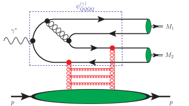
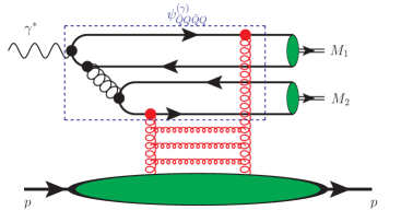
Figure 1: Main classes of diagrams which contribute in the leading order over $\alpha_{s}\left(m_{Q}\right)$ to exclusive photoproduction of quarkonia pairs (type-$A$ and type-$B$ diagrams). The eikonal interactions are shown schematically as exchanges of $t$-channel gluons, indicated by the red wavy lines. In both plots it is implied: (a) summation over all possible attachments of $t$-channel gluons to partons in the upper part of diagram (b) inclusion of diagrams with inverted direction of heavy quark lines (“charge conjugation”). In the right diagram the $t$-channel gluons must be connected to different quark loops in order to guarantee a color singlet $\bar{Q}Q$ in the final state. The blue dashed rectangle schematically shows part of the diagrams which (in absence of eikonal interactions) contribute to the $\bar{Q}Q\bar{Q}Q$-component of the photon wave function $\psi_{\bar{Q}Q\bar{Q}Q}^{(\gamma)}$.

$$\mathcal{A}\left(y_{1},\boldsymbol{p}_{1}^{\perp},y_{2},\boldsymbol{p}_{2}^{\perp}\right) =\mathcal{A}_{1}\left(y_{1},\boldsymbol{p}_{1}^{\perp},y_{2},\boldsymbol{p}_{2}^{\perp}\right)+\mathcal{A}_{2}\left(y_{1},\boldsymbol{p}_{1}^{\perp},y_{2},\boldsymbol{p}_{2}^{\perp}\right),$$ (21)

where $\mathcal{A}_{1}$ and $\mathcal{A}_{2}$ stand for contributions of all type-$A$ and type-$B$ diagrams. Explicitly, these amplitudes are given by

$$\mathcal{A}_{1}\left(y_{1},\boldsymbol{p}_{1}^{\perp},y_{2},\boldsymbol{p}_{2}^{\perp}\right) =\prod_{i=1}^{4}\left(\int d\alpha_{i}d^{2}\boldsymbol{x}_{i}\right)\delta\left(\sum_{k}\alpha_{k}-1\right)\tilde{\sum}_{\ell n}\sigma_{\ell}\sigma_{n}\,c_{\ell n}\gamma\left(\boldsymbol{b}_{\ell}\right)\gamma\left(\boldsymbol{b}_{n}\right)\times$$ (22)

$$\times\left[\Psi_{M_{1}}^{\dagger}\left(\alpha_{14},\,\boldsymbol{r}_{14}\right)\Psi_{M_{2}}^{\dagger}\left(\alpha_{23},\,\boldsymbol{r}_{23}\right)e^{i\left(\boldsymbol{p}_{1}^{\perp}\cdot\boldsymbol{b}_{14}+\boldsymbol{p}_{2}^{\perp}\cdot\boldsymbol{b}_{23}\right)}\delta\left(y_{1}-\mathcal{Y}_{14}\right)\delta\left(y_{2}-\mathcal{Y}_{23}\right)\right.$$

$$+\left.\Psi_{M_{1}}^{\dagger}\left(\alpha_{23},\,\boldsymbol{r}_{23}\right)\Psi_{M_{2}}^{\dagger}\left(\alpha_{14},\,\boldsymbol{r}_{14}\right)e^{i\left(\boldsymbol{p}_{1}^{\perp}\cdot\boldsymbol{b}_{23}+\boldsymbol{p}_{2}^{\perp}\cdot\boldsymbol{b}_{14}\right)}\delta\left(y_{1}-\mathcal{Y}_{23}\right)\delta\left(y_{2}-\mathcal{Y}_{14}\right)\right]$$

$$\times\psi_{\bar{Q}Q\bar{Q}Q}^{(\gamma)}\left(\alpha_{1},\boldsymbol{x}_{1};\,\alpha_{2},\,\boldsymbol{x}_{2};\,\alpha_{3},\,\boldsymbol{x}_{3};\,\alpha_{4},\,\boldsymbol{x}_{4};\,q\right).$$

$$\mathcal{A}_{2}\left(y_{1},\boldsymbol{p}_{1}^{\perp},y_{2},\boldsymbol{p}_{2}^{\perp}\right) =\prod_{i=1}^{4}\left(\int d\alpha_{i}d^{2}\boldsymbol{x}_{i}\right)\delta\left(\sum_{k}\alpha_{k}-1\right)\tilde{\sum}_{\ell n}\sigma_{\ell}\sigma_{n}\,c_{\ell n}\gamma\left(\boldsymbol{b}_{\ell}\right)\gamma\left(\boldsymbol{b}_{n}\right)\times$$ (23)

$$\times\left[\Psi_{M_{1}}^{\dagger}\left(\alpha_{12},\,\boldsymbol{r}_{12}\right)\Psi_{M_{2}}^{\dagger}\left(\alpha_{34},\,\boldsymbol{r}_{34}\right)e^{i\left(\boldsymbol{p}_{1}^{\perp}\cdot\boldsymbol{b}_{12}+\boldsymbol{p}_{2}^{\perp}\cdot\boldsymbol{b}_{34}\right)}\delta\left(y_{1}-\mathcal{Y}_{12}\right)\delta\left(y_{2}-\mathcal{Y}_{34}\right)\right.$$

$$+\left.\Psi_{M_{1}}^{\dagger}\left(\alpha_{34},\,\boldsymbol{r}_{34}\right)\Psi_{M_{2}}^{\dagger}\left(\alpha_{12},\,\boldsymbol{r}_{12}\right)e^{i\left(\boldsymbol{p}_{1}^{\perp}\cdot\boldsymbol{b}_{34}+\boldsymbol{p}_{2}^{\perp}\cdot\boldsymbol{b}_{12}\right)}\delta\left(y_{1}-\mathcal{Y}_{34}\right)\delta\left(y_{2}-\mathcal{Y}_{12}\right)\right]$$

$$\times\psi_{\gamma^{*}\to\bar{Q}Q\bar{Q}Q}\left(\alpha_{1},\boldsymbol{x}_{1};\,\alpha_{2},\,\boldsymbol{x}_{2};\,\alpha_{3},\,\boldsymbol{x}_{3};\,\alpha_{4},\,\boldsymbol{x}_{4};\,q\right),$$

where in the expressions (22, 23) we introduced a few shorthand notations, which characterize the pair of heavy partons $i$ and $j$: the relative distance between them $\boldsymbol{r}_{ij}=\boldsymbol{x}_{i}-\boldsymbol{x}_{j}$, the light-cone fraction $\alpha_{ij}=\alpha_{i}/\left(\alpha_{i}+\alpha_{j}\right)$ carried by the quark in the pair ($ij$), and the transverse coordinate of its center of mass $\boldsymbol{b}_{ij}=\left(\alpha_{i}\boldsymbol{x}_{i}+\alpha_{j}\boldsymbol{x}_{j}\right)/\left(\alpha_{i}+\alpha_{j}\right)$. The notation $\tilde{\sum}_{\ell n}$ in the first line of (22, 23) implies summation over all possible attachments of $t$-channel gluons to the partons in the upper part of the diagram. For type-$A$ diagrams the variables $\ell,\,n$ may take independently six different values, which correspond to connections to final quarks, virtual quark or virtual gluon. For type-$B$ diagrams both produced quark pairs must be in a color singlet state, which translates into the additional constraint that $\ell,\,n$ should be connected to different quark loops (either upper or lower quark-antiquark pairs). The factors $\sigma_{\ell},\,\sigma_{n}$ in the first line of (22, 23) have the value $+1$ if the corresponding $t$-channel gluon is connected to a quark line or gluon, and -1 otherwise. On the other hand, the color factors $c_{\ell n}$ depend on the topology of the diagram under consideration; more precisely, how the $t$-channel gluons are connected to the quark lines. For type-$A$ diagrams, the color factor $c_{\ell n}=\mathcal{C}_{1}\equiv\frac{1}{N_{c}^{2}-1}{\rm tr}_{c}(t_{a}t_{a}t_{b}t_{b})=\left(N_{c}^{2}-1\right)/4N_{c}$, if both $t$-channel gluons are connected to the same quark line, or quark and antiquark lines of opposite color (e.g. quark-antiquark lines originating from colorless photon or leading to formation of colorless quarkonium). If the vertices of the $t$-channel gluons are separated by color changing vertex of a virtual gluon, then the color factor is given by $c_{\ell n}=\mathcal{C}_{2}\equiv\frac{1}{N_{c}^{2}-1}{\rm tr}_{c}(t_{a}t_{b}t_{a}t_{b})=-1/4N_{c}$. For the diagrams with one 3-gluon vertex, when one of the $t$-channel gluons is attached to a virtual gluon, the corresponding color factor is $c_{\ell n}=\pm\mathcal{C}_{3}=\pm N_{c}/4$, where the sign is positive for the diagram with attachment of the other $t$-channel gluon to the upper quark-antiquark pair (i.e. partons 1,2), and negative otherwise. Finally, for the diagram when both $t$-channel gluons are attached to a virtual (intermediate) gluon, the corresponding factor is $c_{\ell n}=\mathcal{C}_{4}\equiv N_{c}/2$. For type-$B$ diagrams, the corresponding color factor is $c_{\ell n}=\frac{1}{N_{c}^{2}-1}\left[{\rm tr}_{c}\left(t_{a}t_{c}\right)\right]^{2}=\frac{1}{4}$ for all possible connections of $t$-channel gluons. The functions $\gamma(...)$ characterize the interaction of the parton with the target, and can be related to the dipole amplitude as explained in Appendix (A). The variables $\boldsymbol{b}_{\ell},\,\boldsymbol{b}_{n}$ in the arguments of $\gamma(...)$-functions stand for the transverse coordinate of the parton which interacts with a $t$-channel gluon. For the final quarks this variable corresponds to the transverse coordinates of these partons (the integration variables $\boldsymbol{x}_{i}$). For intermediate partons this variable is the position of the center of mass of all final quarks which are produced at later stages,

$$\boldsymbol{b}_{j_{1}...j_{n}}=\frac{\sum_{j=j_{1}...j_{n}}\alpha_{j}\boldsymbol{x}_{j}}{\sum_{j=j_{1}...j_{n}}\alpha_{j}}$$ (24)

where the summation is done over all final quarks $j_{1},\,...j_{n}$ which stem from a given parton. The notations $\Psi_{M_{1}},\,\Psi_{M_{2}}$ are used for the wave functions of the final state quarkonia $M_{1}$ and $M_{2}$ (for a moment we disregard completely their spin indices), and $\psi_{\bar{Q}Q\bar{Q}Q}^{(\gamma)}\left(\left\{\alpha_{i},\boldsymbol{x}_{i}\right\};q\right)$ is the 4-quark light-cone wave function of the virtual photon $\gamma^{*}$, which is evaluated in Appendix B.2. The product $\tilde{\sum}_{\ell n}\sigma_{\ell}\sigma_{n}\,c_{\ell n}\gamma\left(\boldsymbol{b}_{\ell}\right)\gamma\left(\boldsymbol{b}_{n}\right)$ can be expressed as a linear superposition of the color singlet dipole amplitudes $N\left(x,\boldsymbol{r}_{ij},\,\boldsymbol{b}_{ij}\right)$ (see derivation in Appendix C). For the type-$A$ contribution, the final result is

$$\tilde{\sum}_{\ell n}\sigma_{\ell}\sigma_{n}\,c_{\ell n}\gamma\left(\boldsymbol{b}_{\ell}\right)\gamma\left(\boldsymbol{b}_{n}\right) =\left\{\frac{2-N_{c}^{2}}{4N_{c}}N\left(x,\,\boldsymbol{r}_{14},\,\boldsymbol{b}_{14}\right)-\frac{1}{2N_{c}}N\left(x,\,\boldsymbol{r}_{34},\,\boldsymbol{b}_{34}\right)-\frac{3+5N_{c}^{2}}{4N_{c}}N\left(x,\,\boldsymbol{r}_{12},\,\boldsymbol{b}_{12}\right)+\right.$$ (25)

$$+\frac{1}{4N_{c}}\left[N\left(x,\,\boldsymbol{r}_{23},\,\boldsymbol{b}_{23}\right)-N\left(x,\,\frac{\alpha_{1}\boldsymbol{r}_{14}+\alpha_{3}\boldsymbol{r}_{34}}{1-\alpha_{2}},\,\boldsymbol{b}_{1344}\right)\right]$$

$$+\frac{N_{c}^{2}+2}{4N_{c}}N\left(x,\,\boldsymbol{r}_{13},\,\boldsymbol{b}_{13}\right)+\frac{3N_{c}^{2}-2}{4N_{c}}\,N\left(x,\frac{\alpha_{1}\boldsymbol{r}_{21}+\alpha_{3}\boldsymbol{r}_{23}+\alpha_{4}\boldsymbol{r}_{24}}{1-\alpha_{2}},\boldsymbol{b}_{1234}\right)$$

$$+\frac{3N_{c}}{2}N\left(x,\frac{\alpha_{3}\boldsymbol{r}_{13}+\alpha_{4}\boldsymbol{r}_{14}}{\alpha_{3}+\alpha_{4}},\boldsymbol{b}_{134}\right)+2N_{c}\,N\left(x,\frac{\alpha_{3}\boldsymbol{r}_{23}+\alpha_{4}\boldsymbol{r}_{24}}{\alpha_{3}+\alpha_{4}},\boldsymbol{b}_{234}\right)$$

$$+\frac{N_{c}^{2}+1}{4N_{c}}\left[N\left(x,\frac{\alpha_{3}\boldsymbol{r}_{13}+\alpha_{4}\boldsymbol{r}_{14}}{1-\alpha_{2}},\boldsymbol{b}_{1134}\right)+N\left(x,\,\boldsymbol{r}_{24},\,\boldsymbol{b}_{24}\right)\right]$$

$$-\frac{N_{c}}{2}\left[N\left(x,\frac{\alpha_{4}\boldsymbol{r}_{34}}{\alpha_{3}+\alpha_{4}},\boldsymbol{b}_{334}\right)+N\left(x,-\frac{\alpha_{3}\boldsymbol{r}_{34}}{\alpha_{3}+\alpha_{4}},\boldsymbol{b}_{344}\right)\right]$$

$$-\frac{N_{c}}{2}\,N\left(x,-\frac{\alpha_{1}\left(\alpha_{3}\boldsymbol{r}_{13}+\alpha_{4}\boldsymbol{r}_{14}\right)}{\left(\alpha_{3}+\alpha_{4}\right)\left(\alpha_{1}+\alpha_{3}+\alpha_{4}\right)},\boldsymbol{b}_{34,134}\right)$$

$$-\left.\frac{N_{c}^{2}-1}{4N_{c}}N\left(x,\,\frac{\alpha_{1}\boldsymbol{r}_{31}+\alpha_{4}\boldsymbol{r}_{34}}{1-\alpha_{2}},\,\boldsymbol{b}_{1334}\right)\right\},$$

whereas for the type-$B$ contribution it is given by

$$\tilde{\sum}_{\ell n}\sigma_{\ell}\sigma_{n}\,c_{\ell n}\gamma\left(\boldsymbol{b}_{\ell}\right)\gamma\left(\boldsymbol{b}_{n}\right) =\frac{1}{4}\left[N\left(x,\boldsymbol{r}_{23},\boldsymbol{b}_{23}\right)-N\left(x,\boldsymbol{r}_{24},\boldsymbol{b}_{24}\right)+N\left(x,\boldsymbol{r}_{3,234},\boldsymbol{b}_{2334}\right)-N\left(x,\boldsymbol{r}_{4,234},\boldsymbol{b}_{2344}\right)+\right.$$ (26)

$$+\left.2N\left(x,\boldsymbol{r}_{14},\boldsymbol{b}_{24}\right)-2N\left(x,\boldsymbol{r}_{13},\boldsymbol{b}_{13}\right)\right]$$

The variables $\mathcal{Y}_{ij}$ in (22, 23) stand for the lab-frame rapidity of quark-antiquark pair made of partons $i,\,j$. Explicitly it is given by

$$\mathcal{Y}_{ij}=\ln\left(\frac{\left(\alpha_{i}+\alpha_{j}\right)q^{+}}{M_{\perp}}\right),$$ (27)

where $\alpha_{i}$ and $\alpha_{j}$ are light-cone fractions of the heavy quarks which form a given quarkonium.

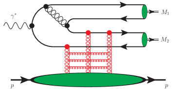
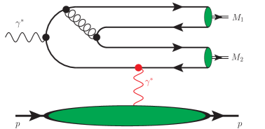
Figure 2: Examples of higher order contributions, which become relevant for the exclusive production of quarkonia with the same $C$-parity. The left diagram corresponds to exchange of odderon (3-gluon ladder) in the $t$-channel, whereas the right diagram corresponds to photon exchange in the $t$-channel. In both plots it is implied summation over all possible attachments of $t$-channel gluons and photon (red) to black-colored partonic lines. As explained in the text, both types of contributions are suppressed compared to diagrams from Figure 1 and will be disregarded in what follows.

The dipole amplitude, which appears in (25,26), effectively takes into account a sum of different pomeron ladders Kovchegov:1999yj ; Kovchegov:2012mbw , and for this reason it corresponds to exchange of vacuum quantum numbers in the $t$-channel. This fact imposes certain constraints on possible quantum numbers of heavy quarkonia produced via the $\gamma+IP\to M_{1}M_{2}$ subprocess. Since the $C$-parity of a photon is negative, the neutral quarkonia $M_{1},\,M_{2}$ must have opposite $C$-parities. This explicitly excludes production of quarkonia with the same quantum numbers ($M_{1}=M_{2}$). For the case when quarkonia are charged (e.g. $B_{c}^{+}B_{c}^{-}$), this implies that they necessarily must be produced with odd value of the mutual angular momentum $L$ . Finally, we need to mention that at higher orders the interaction with the target should be supplemented by the exchange of $C$-odd three-gluon ladders (so-called odderons) in the $t$-channel Hatta:2005as potentially giving contributions of odderon exchange, as shown in the right panel of Figure 2. Such interactions are suppressed at high energies, because the odderon has a smaller intercept than the pomeron. Besides, formally such contribution is also suppressed by $\mathcal{O}\left(\alpha_{s}(m_{Q})\right)$. Another possibility to produce $C$-even pair of quarkonia is via exchange of a ($C$-odd) photon, as shown in the right panel of Figure 2. Formally such contributions are suppressed by $\sim\alpha_{{\rm em}}/\alpha_{s}^{2}\left(m_{Q}\right)$, which is a small parameter for charm and bottom quarks, yet could get enhanced in the infinitely heavy quark mass limit $m_{Q}\to\infty$ due to suppression of $\alpha_{s}\left(m_{Q}\right)$ in the denominator. Besides, this contribution can be enhanced in the very forward kinematics by the photon propagator $\sim 1/t$, where $t\equiv\left(p_{f}-p_{i}\right)^{2}$ is very small . According to phenomenological analyses  Goncalves:2015sfy ; Goncalves:2019txs ; Goncalves:2006hu ; Baranov:2012vu ; Yang:2020xkl , the cross-sections of this mechanism numerically is much smaller than that of the mechanism suggested in this paper. For this reason in what follows we will focus on the production of opposite-parity quarkonia, and will disregard the contributions of $t$-channel odderons and photons altogether.

III Numerical results

The framework developed in the previous section is valid for heavy quarkonia of both $c$ and $b$ flavors. In what follows we will focus on the all-charm sector and present results for $J/\psi+\eta_{c}$ production, for which the cross-section is larger and thus is easier to study experimentally .

For the wave function of the $J/\psi$-mesons we will use a simple ansatz suggested in Dosch:1996ss ; BoostedGaussian ,

$$\Psi_{J/\psi}\left(z,\boldsymbol{r},M=0\right)=\frac{\delta_{h,-\bar{h}}}{\sqrt{2}}z(1-z)\varphi\left(z,\,\boldsymbol{r}\right),\qquad\varphi(z,\,\boldsymbol{r})=\frac{\sqrt{2}\pi f_{V}}{\sqrt{N_{c}}\hat{e}_{V}}f(z)e^{-\omega^{2}r^{2}/2},$$ (28)

$$\Psi_{J/\psi}\left(z,\boldsymbol{r},M=\pm 1\right)=\frac{1}{M_{V}}\left[iMe^{iM\theta}\left(\bar{z}\delta_{h,-M}\delta_{\bar{h},M}-z\delta_{h,M}\delta_{\bar{h},-M}\right)\partial_{r}+m_{Q}\delta_{h,M}\delta_{\bar{h},M}\right]\varphi\left(z,\,\boldsymbol{r}\right)$$ (29)

$$f(z)=\sqrt{z(1-z)}e^{-M_{V}^{2}\left(z-1/2\right)^{2}/2\omega^{2}}$$ (30)

where $M$ is the helicity of $J/\psi$, $\boldsymbol{r}$ is the distance between the quark and antiquark, $h,\,\bar{h}$ are the helicities of the quark and antiquark, and $f_{V},e_{V},\,\omega$ are some numerical constants. This result can be trivially extended to the case of $\eta_{c}$-meson, which differs from the $J/\psi$ meson only by the orientation of the quark spins. Taking into account the structure of the Clebsch-Gordan coefficients for the $1/2\times 1/2$ product, we may immediately write out the corresponding wave functions for $\eta_{c}$, modifying the corresponding $M=0$ component of the $J/\psi$ wave function,

$$\Psi{}_{\eta_{c}}\left(z,\boldsymbol{r}\right) =\frac{\varepsilon_{h,\bar{h}}}{\sqrt{2}}z(1-z)\varphi\left(z,\,\boldsymbol{r}\right),\qquad\varepsilon_{ab}=-\varepsilon_{ba}=\delta_{a,-b}{\rm sign}(a).$$ (31)

Alternatively, the wave functions of quarkonia can be constructed using potential models or the well-known Brodsky-Huang-Lepage-Terentyev (BHLT) prescription BHT ; Brodsky:2003pw ; Terentev:1976jk which allows to convert the rest frame wave function $\psi_{{\rm RF}}$ into a light-cone wave function $\Psi_{{\rm LC}}$. It is known that in the small-$r$ region, which is relevant for estimates, the wave functions of the $S$-wave heavy quarkonia in different schemes are quite close to each other Stadler:2018hjv ; Daniel:1990ah ; Kawanai:2011xb ; Kawanai:2013aca , and for this reason in what follows we will use the ansatz of (28-31), in view of its simplicity.

For our numerical evaluations we also need a parametrization of the dipole amplitude. In what follows we will we use the impact parameter ($b$) dependent “bCGC” parametrization of the dipole cross-section Kowalski:2006hc ; RESH ,

$$N\left(x,\,\boldsymbol{r},\,\boldsymbol{b}\right) =\left\{\begin{array}[]{cc}N_{0}\,\left(\frac{r\,Q_{s}(x)}{2}\right)^{2\gamma_{{\rm eff}}(r)},&r\,\leq\frac{2}{Q_{s}(x)}\\ 1-\exp\left(-\mathcal{A}\,\ln\left(\mathcal{B}r\,Q_{s}\right)\right),&r\,>\frac{2}{Q_{s}(x)}\end{array}\right.\leavevmode\nobreak\ ,$$ (34)

$$\mathcal{A}=-\frac{N_{0}^{2}\gamma_{s}^{2}}{\left(1-N_{0}\right)^{2}\ln\left(1-N_{0}\right)},\quad\mathcal{B}=\frac{1}{2}\left(1-N_{0}\right)^{-\frac{1-N_{0}}{N_{0}\gamma_{s}}},$$ (35)

$$Q_{s}(x,\,\boldsymbol{b})=\left(\frac{x_{0}}{x}\right)^{\lambda/2}T_{G}(b),\,\,\gamma_{{\rm eff}}(r)=\gamma_{s}+\frac{1}{\kappa\lambda Y}\ln\left(\frac{2}{r\,Q_{s}(x)}\right),$$ (36)

$$\gamma_{s} =0.66,\quad\lambda=0.206,\quad x_{0}=1.05\times 10^{-3},\quad T_{G}(b)=\exp\left(-\frac{b^{2}}{2\gamma_{s}B_{{\rm CGC}}}\right).$$ (37)

We would like to start the presentation of numerical results from a discussion of the relative contribution of type-$A$ and type-$B$ diagrams introduced in the previous section. From the left panel of Figure 3 we can see that the dominant contribution comes from the type-$A$ diagrams. Partially this enhancement can be explained by larger color factors in the large-$N_{c}$ limit. The interference of type-$A$ and type-$B$ contributions represents approximately a 10% correction and moreover, has a node, whose position depends on the produced quarkonia kinematics. As expected, the cross-section is suppressed as a function of $p_{T}$ (we considered $\left|\boldsymbol{p}_{J/\psi}^{\perp}\right|=\left|\boldsymbol{p}_{\eta}^{\perp}\right|=p_{T}$ for the sake of definiteness). In the right panel of the same Figure 1 we present the dependence of the yields on the azimuthal angle $\phi$ between the transverse momenta of the $J/\psi$ and $\eta_{c}$ mesons. For definiteness, we assumed that the transverse momenta $\boldsymbol{p}_{J/\psi}^{\perp},\,\boldsymbol{p}_{\eta}^{\perp}$ of both quarkonia have equal absolute values. In order to make meaningful comparison of the cross-sections, which differ by orders of magnitude, we plotted the normalized ratio

$$R(\phi) =\frac{d\sigma\left(...,\,\phi\right)/dy_{1}dp_{1}^{2}dy_{2}dp_{2}^{2}d\phi}{d\sigma\left(...,\,\phi=\pi\right)/ddy_{1}dp_{1}^{2}dy_{2}dp_{2}^{2}d\phi},\qquad R(\phi=\pi)\equiv 1$$ (38)

We can see that the ratio has a sharp peak in the back-to-back region ($\phi=\pi$), which happens because in this kinematics the momentum transfer to the target $|t|=\left|\Delta^{2}\right|$ is minimal. In contrast, for the angle $\phi\approx 0$, which maximizes the variable $|t|=\left|\Delta^{2}\right|$, the ratio has a pronounced dip. For $p_{1}\not=p_{2}$ the dependence on $\phi$ is qualitatively similar, although the maximum and minimum are less pronounced.

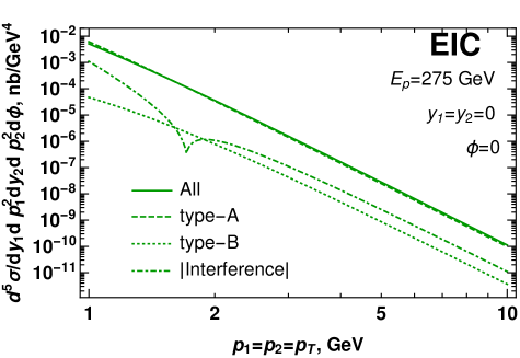
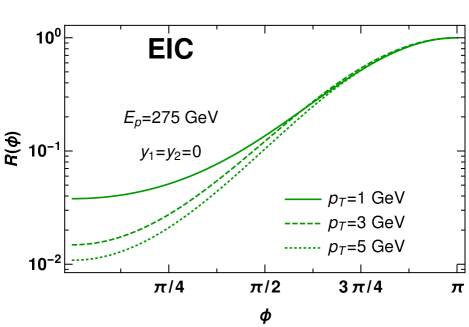
Figure 3: Left plot: Different contributions to charmonia pair photoproduction in EIC kinematics: the type-$A$ and type-$B$ diagrams, as well as their interference. Right plot: The dependence of the normalized ratio $R(\phi)$, defined in (38), on the angle $\phi$ (difference between azimuthal angles of both quarkonia). The appearance of a sharp peak in back-to-back kinematics is explained in the text. For definiteness we considered the case when both quarkonia are produced at central rapidities ($y_{1}=y_{2}=0$) in the lab frame; for other rapidities the $\phi$-dependence has a similar shape.

In the left panel of the Figure 4 we analyze the $p_{T}$-dependence, for the case when one of the quarkonia has a small transverse momentum $p_{i}\sim 1\,{\rm GeV}$. As expected, in this case the cross-section has a significantly milder suppression compared to the case when both quarkonia share the same transverse momentum. This result indicates that the quarkonia pair are predominantly produced with small transverse momenta $p_{1}^{\perp}\sim p_{2}^{\perp}\lesssim 1\,{\rm GeV}$ and opposite directions in the transverse plane ( $\phi\equiv\phi_{1}-\phi_{2}\approx\pi$). In the right panel of the same Figure 4, we show the $p_{T}$-dependence of the cross-section in LHeC kinematics. While the absolute value increases in this case, we may observe that qualitatively the dependence on $p_{T}$ and angle $\phi$ remains the same.

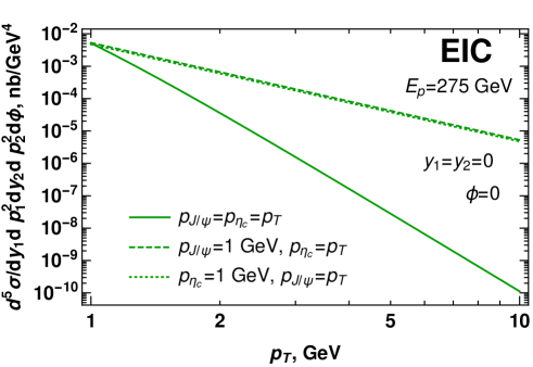
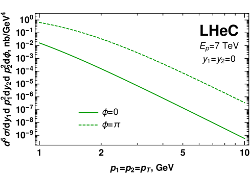
Figure 4: Left plot: The $p_{T}$-dependence of the charmonia pair photoproduction cross-section. Comparison of the case when both quarkonia have large transverse momentum (solid line), with the cases when one of the produced quarkonia is small (dashed and dot-dashed lines). Within errors of numerical evaluation, there is no difference if the soft transverse momentum $p_{T}\approx 1\,{\rm GeV}$ is assigned to $J/\psi$ or $\eta_{c}$ mesons. Right plot: The $p_{T}$-dependence of the cross-section in LHeC kinematics. For definiteness we considered the case when both quarkonia are produced at central rapidities ($y_{1}=y_{2}=0$) in the lab frame.

In Figure 5 we analyze the dependence of the cross-section on rapidities of the quarkonia. In the left panel we consider the special case when both quarkonia are produced with the same transverse momenta $p_{1}^{\perp}\sim p_{2}^{\perp}\sim 1\,{\rm GeV}$ and the same rapidities $y_{1}=y_{2}$ in the lab frame. The variables $y_{1,2}$ in this case can be unambiguously related to the invariant photon-proton energy $W_{\gamma p}\sim\sqrt{s_{\gamma p}}$ (shown in the upper horizontal axis), and as expected, the cross-section grows as a function of energy. In the right panel of the same Figure  5 we analyze the dependence of the cross-section on the rapidity difference $\Delta y$ between two heavy mesons. For the sake of definiteness we consider that both quarkonia have opposite rapidities in the lab frame, $y_{1}=-y_{2}=\Delta y/2$. We observe that in this case the cross-section becomes suppressed as a function of $\Delta y$, which illustrates the fact that the quarkonia are predominantly produced with the same rapidities.

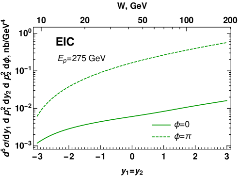
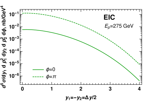
Figure 5: Left plot: The rapidity dependence of the photoproduction cross-section in EIC kinematics, assuming equal rapidities of the produced quarkonia, $y_{1}=y_{2}$. The upper horizontal scale illustrates the corresponding value of invariant energy $W\equiv\sqrt{s_{\gamma p}}$ defined in (14). Right plot: The dependence on the rapidity difference between the produced quarkonia, $y_{1}=-y_{2}=\Delta y/2$. For the sake of definiteness we assumed that both quarkonia are produced at central rapidities ($y_{1}=y_{2}=0$) with transverse momenta $p_{1}=p_{2}=1$ GeV in the lab frame.

Finally, in Figures 6, 7, 8 we show the results for the cross-section $d\sigma_{\gamma p\to M_{1}M_{2}p}/dy_{1}dy_{2}$, which is integrated over transverse momenta $\boldsymbol{p}_{i}^{\perp}$ of both quarkonia. This observable can be the most promising for experimental studies, since it is easier to measure. We make the predictions in the kinematics of the ultraperipheral $pA$ collisions at LHC, as well as future electron-hadron colliders. Largely, the dependence on $y_{1},\,y_{2}$ repeats similar dependence of the $p_{T}$-unintegrated cross-sections. This happens because the $p_{T}$-integrated cross-sections get its dominant contributions from the region of small $p_{T}\ll m_{Q}$, where dependence on rapidity is mild. In Figures 6, 7 we have also shown the cross-sections of “master” processes $ep\to eM_{1}M_{2}p$ and $Ap\to AM_{1}M_{2}p$. The expressions for these cross-sections differ from those of $\gamma p\to M_{1}M_{2}p$ by a convolution with known kinematic factors, which correspond to fluxes of equivalent photons generated by the electron or heavy nucleus. These cross-sections have completely different behavior on the rapidity $y_{1}=y_{2}$ of both quarkonia, which can be understood from (8-16). Indeed, mesons with higher lab-frame rapidities can be produced by photons of higher energy $E_{\gamma}$, yet the flux of equivalent photons created by a charged electron or ion is suppressed and vanishes when the elasticity $y=E_{\gamma}/E_{e}$ approaches unity. Finally, Figure 8 illustrates how the cross-section behaves as a function of $y_{1},y_{2}$ in general, when $|y_{1}|\not=|y_{2}|$. We can see that the cross-section has a typical ridge near $y_{1}\approx y_{2}$, i.e. when quarkonia are produced with approximately the same rapidities.

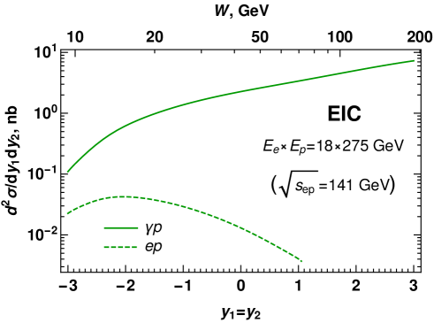
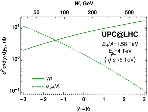
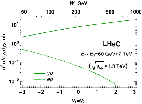
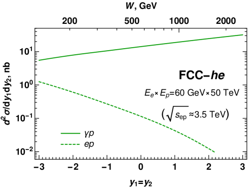
Figure 6: The rapidity dependence of the $p_{T}$-integrated cross-section in the kinematics of ultraperipheral collisions at LHC and in the kinematics of the future $ep$ colliders. A positive sign of rapidity is chosen in the direction of electron or emitted quasi-real photon. For UPC collisions the positive direction of rapidity is that of a heavy lead ion, and the cross-sections are given per nucleon. The solid curves correspond to cross-section of the $\gamma p\to M_{1}M_{2}p$ subprocess, whereas dotted lines correspond to the cross-sections of the complete physically observable $ep$ or $Ap$ processes. We assume for definiteness that the rapidities of both quarkonia are equal to each other in the lab frame, $y_{1}=y_{2}=y$. The upper horizontal scale illustrates the corresponding value of invariant energy $W\equiv\sqrt{s_{\gamma p}}$, as defined in (14).

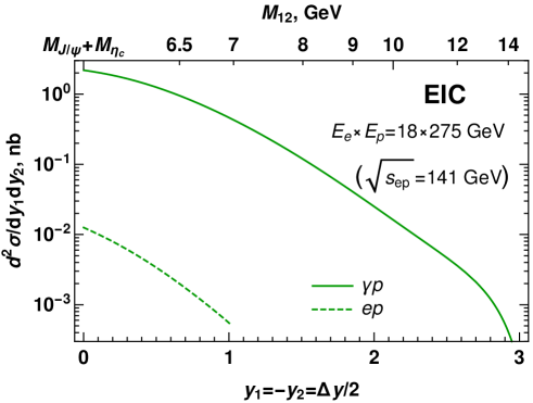
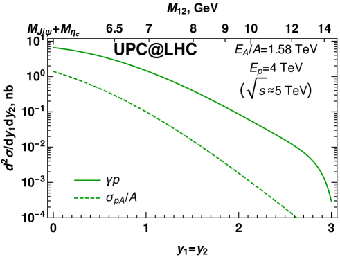
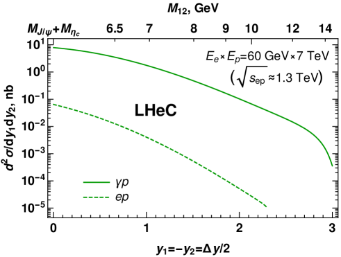
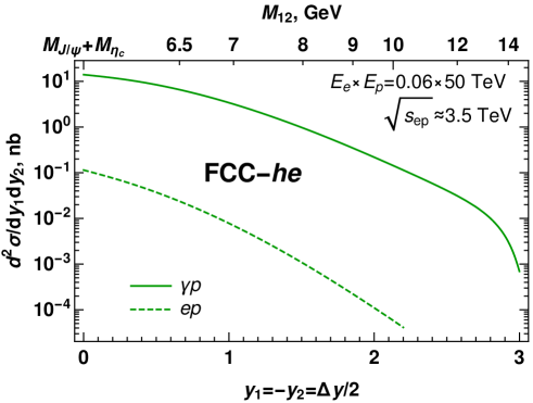
Figure 7: The dependence on rapidity difference for the $p_{T}$-integrated cross-section, in the kinematics of ultraperipheral collisions, at LHC and future electron-proton colliders. The positive sign of rapidity is chosen in the direction of electron or emitted quasi-real photon. For UPC collisions the positive direction of rapidity is that of a heavy lead ion, and the cross-sections are given per nucleon. For the sake of definiteness we assume that in the lab frame the quarkonia have opposite rapidities, $y_{1}=-y_{2}=\Delta y/2$. The upper horizontal scale illustrates the corresponding value of the invariant mass $M_{12}\equiv\sqrt{\left(p_{J/\psi}+p_{\eta_{c}}\right)^{2}}$, as defined in (15). Dotted curves correspond to the cross-sections of the complete process (electron-proton or heavy ion-proton).

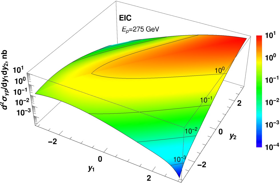
Figure 8: (Color online) The dependence on rapidities $y_{1},\,y_{2}$, of produced quarkonia, for the $p_{T}$-integrated photoproduction cross-section $d\sigma_{\gamma p}/dy_{1}dy_{2}$. The plot illustrates the fact that partons are produced with approximately equal rapidities, $y_{1}\approx y_{2}$. For definiteness we consider the proton with a typical energy of EIC kinematics ($E_{p}\sim 275$ GeV in the lab frame). For other proton energies the dependence has qualitatively similar shape.

IV Conclusions

In this paper we studied in detail the exclusive photoproduction of heavy charmonia pairs. This process presents a lot of interest, both on its own, as a potential test of quarkonia production mechanisms in small-$x$ kinematics, as well as a background to exotic hadron production. We analyzed in detail the leading order contributions and found that in this mechanism the quarkonia pairs are produced with opposite $C$-parities, relatively small opposite transverse momenta $p_{T}$, and small separation in rapidity. This finding is explained by the fact that in the chosen kinematical region the momentum transfer to the recoil proton is minimal. As expected, the cross-section decreases rapidly as a function of $p_{T}$, and grows as a function of photon-proton invariant energy ($\sim$quarkonia rapidities), similar to single-photon production. However, the cross-section decreases as a function of the rapidity difference between the quarkonia. We estimated numerically the cross-section in the kinematics of ultraperipheral $pA$ collisions at LHC, as well as in the kinematics of the future electron-proton colliders, and found that the cross-section is sufficiently large for experimental studies. Our evaluation is largely parameter-free and relies only on the choice of the parametrization for the dipole cross-section (34) and wave functions of quarkonia.

We need to mention that earlier studies of exclusive production focused on production of quarkonia pairs with the same quantum numbers (e.g. $J/\psi\,J/\psi$). In view of different quantum numbers, this process predominantly proceed via exchange of two photons at amplitude level, like e.g. via photon-photon fusion $\gamma\gamma\to M_{1}M_{2}$ Goncalves:2015sfy ; Goncalves:2019txs ; Goncalves:2006hu ; Baranov:2012vu ; Yang:2020xkl or double photon scattering Goncalves:2016ybl . Due to extra virtual photon in the amplitude, the cross-sections of such processes are parametrically suppressed by $\sim\alpha_{{\rm em}}^{2}$ compared to the cross-section of opposite $C$-parity quarkonia, and thus numerically are significantly smaller. We hope that the process suggested in this paper will be included in the program of the future EIC collider, as well as ongoing studies at LHC in ultraperipheral kinematics.

Finally, we need to mention that it is quite straightforward to extend the framework developed in this manuscript to the case of all-heavy tetraquark production: for this it is only necessary that the product of final state quarkonia wave functions in (22, 23) be replaced with the wave function of the tetraquark state. Estimates of the cross-sections for this case will be presented in a separate publication.

Acknowldgements

We thank our colleagues at UTFSM university for encouraging discussions. This research was partially supported by projects Proyecto ANID PIA/APOYO AFB180002 (Chile) and Fondecyt Regular (Chile) grants 1180232 and 1220242. The research of S. Andrade was partially supported by the Fellowship Program ANID BECAS/MAGÍSTER NACIONAL (Chile) 22200123. Powered@NLHPC: This research was partially supported by the supercomputing infrastructure of the NLHPC (ECM-02).

Appendix A High energy scattering in the color dipole picture

In this appendix for the sake of completeness we briefly remind the general procedure which allows to express different hard amplitudes in terms of the color singlet forward dipole scattering amplitude. While in the literature there are several equivalent formulations GLR ; McLerran:1993ka ; McLerran:1994vd ; MUQI ; MV ; gbw01:1 ; Kopeliovich:2002yv ; Kopeliovich:2001ee , in what follows we will use the Iancu-Mueller approach Iancu:2003uh .

The natural hard scale, which controls the interaction of a heavy quark with the gluonic field, is its mass $m_{Q}$. In the heavy quark mass limit we may formally develop a systematic expansion over $\alpha_{s}\left(m_{Q}\right)\ll 1$. Furthermore, for small color singlet dipoles there is an additional suppression by the dipole size, $r\sim 1/m_{Q}$, so the interaction of singlet dipoles with perturbative gluons is suppressed at least as $\sim\alpha_{s}\left(m_{Q}\right)/m_{Q}$. However, the interaction of gluons with each other, as well as with light quarks, remains strongly nonperturbative in the deeply saturated regime, so we expect that the dynamics of the dipole amplitudes should satisfy the nonlinear Balitsky-Kovchegov equation.

At very high energies the dynamics of partons can be described in the eikonal approximation. The transverse coordinates of the high energy partons remain essentially frozen during its propagation in the gluonic field dipole of the target. Similarly, due to eikonal interactions we may disregard completely the change of the quark helicities. In this picture the interaction of a dipole with the target is described by the $S$-matrix element Iancu:2003uh ; Kovchegov:2012mbw

$$S(y,\,\boldsymbol{x}_{Q},\,\boldsymbol{x}_{\bar{Q}})=\frac{1}{N_{c}}\left\langle{\rm tr}\left(V^{\dagger}(\boldsymbol{\boldsymbol{x}_{Q}})V(\boldsymbol{x}_{\bar{Q}})\right)\right\rangle$$ (39)

where we use the notation $y=\ln(1/x)$ for the dipole rapidity, $\boldsymbol{x}_{Q}\,,\boldsymbol{x}_{\bar{Q}}$, are the transverse coordinates of the partons (quark or antiquark), and the factors $V^{\dagger}(\boldsymbol{x}_{Q})$ and $V(\boldsymbol{x}_{\bar{Q}})$ in (39) are the Wilson lines, which describe the interaction of the partons with the color field of a hadron. They can be expressed as

$$V\left(\boldsymbol{x}_{\perp}\right)=P\exp\left(ig\int dx^{-}A_{a}^{+}\left(x^{-},\,\boldsymbol{x}_{\perp}\right)t^{a}\right),$$ (40)

where $A_{\mu}^{a}$ is the gluonic field in a hadron. The impact parameter dependent dipole amplitude $N(x,\,\boldsymbol{r},\,\boldsymbol{b})$ can be related to $S\left(y,\,\boldsymbol{x}_{Q},\,\boldsymbol{x}_{\bar{Q}}\right)$ as

$$N\left(x,\,\boldsymbol{r},\,\boldsymbol{b}\right)=1-S\left(y,\,\boldsymbol{x}_{Q},\,\boldsymbol{x}_{\bar{Q}}\right),$$ (41)

where the variable $\boldsymbol{r}\equiv\boldsymbol{x}_{Q}-\boldsymbol{x}_{\bar{Q}}$ is the transverse size of the dipole, $\boldsymbol{b}\equiv z\,\boldsymbol{x}_{Q}+(1-z)\boldsymbol{x}_{\bar{Q}}$ is the transverse position of the dipole center of mass, and $z$ is the fraction of the light-cone momentum of a dipole which is carried by the quark $Q$. In view of the weakness of the interaction between heavy quarks and gluons, we can make an expansion of the exponent in (40) over $\alpha_{s}(m_{Q})$. In this approximation the effective interaction of the quark or antiquark with the gluonic field of the proton can be described by the factor $\pm i\,t^{a}\gamma_{a}\left(\boldsymbol{x}_{\perp}\right)$, where $\boldsymbol{x}_{\perp}$ is the transverse coordinate of the quark,

$$\gamma_{a}(\boldsymbol{x})=g\int dx^{-}A_{a}^{+}(x^{-},\,\boldsymbol{x}),$$ (42)

and $t_{a}$ are the ordinary color group generators of pQCD in the fundamental representation. Inspired by the color structure of the interaction, in what follows we will refer to these interactions as “exchanges of $t$-channel pomeron (gluons)”, tacitly assuming that it can include cascades (showers) of particles. For the dipole scattering amplitude (41), using (39, 42), we obtain

$$N\left(x,\,\boldsymbol{r},\,\boldsymbol{b}\right)\approx\frac{1}{2}\left[\gamma_{a}\left(\boldsymbol{x}_{Q}\right)-\gamma_{a}\left(\boldsymbol{x}_{\bar{Q}}\right)\right]^{2}.$$ (43)

For further evaluations it is more convenient to rewrite this result in the form

$$\gamma_{a}\left(\boldsymbol{x}_{1}\right)\gamma_{a}\left(\boldsymbol{x}_{2}\right)=-N\left(x,\,\boldsymbol{r}_{12},\,\boldsymbol{b}_{12}\right)+\frac{\rho\left(\boldsymbol{x}_{1}\right)+\rho\left(\boldsymbol{x}_{2}\right)}{2},$$ (44)

where we defined a shorthand notation $\rho\left(\boldsymbol{x}_{a}\right)\equiv\left|\gamma_{a}(\boldsymbol{x})\right|^{2}$, and $\boldsymbol{r}_{12}$, $\boldsymbol{b}_{12}$ are the distance and center-of-mass of the quark-antiquark pair located at points $\boldsymbol{x}_{1},\,\boldsymbol{x}_{2}$. For many processes the contributions $\sim\rho\left(\boldsymbol{x}_{i}\right)$ cancel, so the amplitude eventually can be represented as a linear superposition of the dipole amplitudes $N\left(x,\,\boldsymbol{r},\,\boldsymbol{b}\right)$. In what follows, we will see that the amplitude of the process considered in this manuscript can be represented as a bilinear combination of terms with structure $\sim\left[\gamma\left(\boldsymbol{x}_{i}\right)-\gamma\left(\boldsymbol{x}_{j}\right)\right]$. For this special case the substitution of (44) allows to get a few important identities between bilinear expressions

$$\left[\gamma_{a}\left(\boldsymbol{x}_{1}\right)-\gamma\left(\boldsymbol{x}_{2}\right)\right] \left[\gamma_{a}\left(\boldsymbol{x}_{3}\right)-\gamma_{a}\left(\boldsymbol{x}_{4}\right)\right]=N\left(x,\,\boldsymbol{r}_{23},\,\boldsymbol{b}_{23}\right)+N\left(x,\,\boldsymbol{r}_{14},\,\boldsymbol{b}_{14}\right)-N\left(x,\,\boldsymbol{r}_{13},\,\boldsymbol{b}_{13}\right)-N\left(x,\,\boldsymbol{r}_{24},\,\boldsymbol{b}_{24}\right),$$ (45)

$$\left[\gamma_{a}\left(\boldsymbol{x}_{1}\right)-\gamma_{a}\left(\boldsymbol{x}_{2}\right)\right] \left[\gamma_{a}\left(\boldsymbol{x}_{3}\right)+\gamma_{a}\left(\boldsymbol{x}_{4}\right)-2\gamma_{a}\left(\boldsymbol{x}_{5}\right)\right]=N\left(x,\,\boldsymbol{r}_{23},\,\boldsymbol{b}_{23}\right)+N\left(x,\,\boldsymbol{r}_{24},\,\boldsymbol{b}_{24}\right)-N\left(x,\,\boldsymbol{r}_{13},\,\boldsymbol{b}_{13}\right)-$$ (46)

$$\text{}-N\left(x,\,\boldsymbol{r}_{14},\,\boldsymbol{b}_{14}\right) +2\left[N\left(x,\,\boldsymbol{r}_{15},\,\boldsymbol{b}_{15}\right)-N\left(x,\,\boldsymbol{r}_{25},\,\boldsymbol{b}_{25}\right)\right],$$

$$\left[\gamma_{a}\left(\boldsymbol{x}_{1}\right)+\gamma_{a}\left(\boldsymbol{x}_{2}\right)-2\gamma_{a}\left(\boldsymbol{x}_{3}\right)\right]^{2}=2N\left(x,\,\boldsymbol{r}_{13},\,\boldsymbol{b}_{13}\right)+2N\left(x,\,\boldsymbol{r}_{23},\,\boldsymbol{b}_{23}\right)-N\left(x,\,\boldsymbol{r}_{12},\,\boldsymbol{b}_{12}\right),$$ (47)

where $\boldsymbol{r}_{ij}$ and $\boldsymbol{b}_{ij}$ are the relative distance and center-of-mass of the quark-antiquark pair located at points $\boldsymbol{x}_{i},\,\boldsymbol{x}_{j}$.

For the impact parameter independent ($\boldsymbol{b}$-integrated) cross-section the results (43-45) can be rewritten in a simpler form,

$$N(x,\,\boldsymbol{r})=\frac{1}{2}\int d^{2}b\left|\gamma_{a}\left(x,\,\boldsymbol{b}-z\boldsymbol{r}\right)-\gamma_{a}\left(x,\,\boldsymbol{b}+\bar{z}\boldsymbol{r}\right)\right|^{2}.$$ (48)

$$\int d^{2}\boldsymbol{b}\gamma_{a}(x,\,\boldsymbol{b})\gamma_{a}(x,\,\boldsymbol{b}+\boldsymbol{r})=-N(x,\,\boldsymbol{r})+\underbrace{\int d^{2}b\,\left|\gamma_{a}(x,\,\boldsymbol{b})\right|^{2}}_{={\rm const}}.$$ (49)

The value of the constant term in the right-hand side of (49) is related to the infrared behavior of the theory, and for the observables which we consider in this paper, it cancels exactly. In what follows we will apply this formalism to the evaluation of the exclusive dimeson production amplitudes.

Appendix B Evaluation of the photon wave function

For evaluation of the photon wave function we follow the standard rules of the light–cone perturbaiton theory formulated in Lepage:1980fj ; Brodsky:1997de . The result for the $\bar{Q}Q$ component is well-known in the literature Bjorken:1970ah ; Dosch:1996ss , yet below in Subsection B.1 we will briefly repeat its derivation in order to introduce notations. As we will see later in Subsection B.2, the wave function of the $\bar{Q}Q\bar{Q}Q$-component can be expressed in terms of the wave function of $\bar{Q}Q$-component. In our evaluation we will focus on onshell transversely polarized photons, which give the dominant contribution, unless some specific cuts are imposed on its virtuality $Q^{2}$. The momentum of the photon (1) introduced earlier simplifies in this case and has only light-cone component in the plus-axis direction,

$$q\approx\left(q^{+},\,0,\,\boldsymbol{0}_{\perp}\right).$$ (50)

The polarization vector of the transversely polarized photon is given by

$$\varepsilon_{T}^{\mu}(q) \equiv\left(0,\,\frac{\boldsymbol{q}_{\perp}\cdot\boldsymbol{\boldsymbol{\varepsilon}}_{\gamma}}{q^{+}},\,\boldsymbol{\boldsymbol{\varepsilon}}_{\gamma}\right)\approx\left(0,\,0,\,\boldsymbol{\boldsymbol{\varepsilon}}_{\gamma}\right),$$ (51)

$$\boldsymbol{\boldsymbol{\varepsilon}}_{\gamma} =\frac{1}{\sqrt{2}}\left(\begin{array}[]{c}1\\ \pm i\end{array}\right),\quad\gamma=\pm 1.$$ (54)

where in (51) we took into account that $\boldsymbol{q}_{\perp}=0$.

Before the interaction with the target, the photon might fluctuate into virtual quark-antiquark pairs, as well as gluons. In what follows we will use a convenient shorthand notation $\alpha_{i}=k_{i}/q^{+}$ for the fraction of light-cone momentum of the photon carried by each parton, as well as $\boldsymbol{k}_{i\perp}$for the transverse component of parton’s momentum. In view of 4-momentum conservation we expect that $\alpha_{i},\boldsymbol{k}_{i\perp}$ should satisfy an identity

$$\sum_{i}\alpha_{i} =1,\qquad\sum_{i}\boldsymbol{k}_{i\perp}=0,$$ (55)

where summation is done over all partons. We may observe that the vector $\boldsymbol{\boldsymbol{\varepsilon}}_{\gamma}$ satisfies an identity

$$\boldsymbol{\boldsymbol{\varepsilon}}_{\gamma}^{*}\equiv\boldsymbol{\boldsymbol{\varepsilon}}_{-\gamma},$$ (56)

and its scalar product with any 2-vector $a$ yields

$$\boldsymbol{\boldsymbol{\varepsilon}}_{\gamma}\cdot\boldsymbol{a}=\frac{a_{x}+i\gamma a_{y}}{\sqrt{2}}=\frac{\left|a\right|}{\sqrt{2}}e^{i\gamma\,{\rm arg}(a)},\,\,\,\,{\rm arg}(a)=\arctan\left(\frac{a_{y}}{a_{x}}\right).$$ (57)

B.1 $\bar{Q}Q$ component of the photon wave function

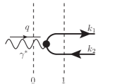
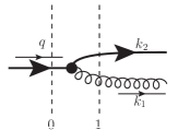
Figure 9: Left plot: The leading order contributions to the $\bar{Q}Q$-component of the photon wave function $\psi_{g\to\bar{Q}Q}$. Right plot: the so-called gluon emission wave function, as defined in Lappi:2016oup . The momenta $k_{i}$ shown in the right-hand side are Fourier conjugates of the coordinates $x_{i}$.

In this section for the sake of completeness we would like to remind the reader the main steps in the derivation of the $\bar{Q}Q$-component photon wave function Bjorken:1970ah ; Dosch:1996ss in the mixed ($\alpha,\,\boldsymbol{r}$) representation. In leading order the subprocess $\gamma\to\bar{Q}Q$ gets contributions only from the diagram shown in the left panel of the Figure 9. A bit later we will see that $\gamma\to\bar{Q}Q$, as well as the closely related $g\to\bar{Q}Q$ subprocess, appears as constituent blocks in the more complicated 4-quark wave function. For this reason, in order to facilitate further discussion, temporarily in this section we will assume that the photon momentum $q$ might has a nonzero transverse part $\boldsymbol{q}_{\perp}$, and will use notation $z=k_{1}^{+}/q^{+}$ for the fraction of light-cone momentum carried by the quark. In momentum space the evaluation is straightforward, using the rules from  Lepage:1980fj ; Brodsky:1997de ; Lappi:2016oup and yields

$$\psi_{h,\bar{h}}^{\lambda}\left(z,\,k_{1},\boldsymbol{q}\right) =-e_{q}\delta_{c\bar{c}}\frac{\bar{u}_{h}\left(k_{1}\right)\hat{\varepsilon}_{\lambda}(q)v_{\bar{h}}\left(q-k_{1}\right)}{\Delta_{01}^{-}\,\,\sqrt{k_{1}^{+}}\sqrt{q^{+}-k_{1}^{+}}}$$ (58)

$$\Delta_{01}^{-} =-\frac{1}{2p^{+}}\,\frac{\boldsymbol{n}^{2}+m_{q}^{2}}{z\,(1-z)},$$ (59)

where $\lambda$ is the helicity of the incoming photon, $h,\,\bar{h}$, are the helicities of the produced quark and antiquark, $c,\,\bar{c}$, are the color indices of $Q$ and $\bar{Q}$, respectively, and $e_{q}$ is the electric charge corresponding to a given heavy flavor. The momentum $\boldsymbol{n}$ is defined as $\boldsymbol{n}=\boldsymbol{k}_{1}-z\boldsymbol{q}_{\perp}=(1-z)\boldsymbol{k}_{1}-z\boldsymbol{k}_{2}$ and physically has the meaning of the transverse part of the relative (internal) momentum of the $Q\bar{Q}$ pair. The numerator of (58) can be written out explicitly using the rules from Bjorken:1970ah ; Dosch:1996ss ,

$$\bar{u}_{h}\left(k\right)\hat{\varepsilon}_{\lambda}(p)v_{\bar{h}}\left(p-k\right) =\frac{2}{\sqrt{z(1-z)}}\left[\left(z\delta_{\lambda,h}-(1-z)\delta_{\lambda,-h}\right)\delta_{h,-\bar{h}}\boldsymbol{n}\cdot\boldsymbol{\varepsilon}_{\lambda}+\frac{1}{\sqrt{2}}m_{q}\,{\rm sign}(h)\delta_{\lambda,h}\delta_{h,\bar{h}}\right].$$ (60)

In configuration space the corresponding wave function can be found making a Fourier transformation over the transverse momenta,

$$\int\frac{d^{2}k_{1}}{(2\pi)^{2}}\frac{d^{2}k_{2}}{(2\pi)^{2}}e^{i\left(\boldsymbol{k}_{1}\cdot\boldsymbol{r}_{1}+\boldsymbol{k}_{2}\cdot\boldsymbol{r}_{2}\right)}\left(2\pi\right)^{2}\delta\left(\boldsymbol{k}_{1}+\boldsymbol{k}_{2}-\boldsymbol{q}\right)\psi_{h,\bar{h}}^{\lambda}\left(z,\,k_{1},\boldsymbol{q}\right)$$ (61)

$$=e^{i\boldsymbol{q}\cdot\left(z\boldsymbol{r}_{1}+\bar{z}\boldsymbol{r}_{2}\right)}e_{q}\delta_{c\bar{c}}\Psi_{h\bar{h}}^{\lambda}\left(z,\,\boldsymbol{r}_{12},\,m_{q},\,m_{q}\right),$$

where the integral over $k_{2}$ was performed using the properties of the $\delta$ function, and before the integration over $\boldsymbol{k}_{1}$ we shifted the integration variable as $\boldsymbol{k}_{1}\to\boldsymbol{n}+z\boldsymbol{q}$. Explicitly, the integration over the variable $d^{2}\boldsymbol{n}$ yields

$$\Psi_{h\bar{h}}^{\lambda}\left(z,\,\boldsymbol{r}_{12},\,m_{q},a\right)=-\frac{2}{(2\pi)}\left[\left(z\delta_{\lambda,h}-(1-z)\delta_{\lambda,-h}\right)\delta_{h,-\bar{h}}i\boldsymbol{\varepsilon}_{\lambda}\cdot\nabla-\frac{m_{q}}{\sqrt{2}}\,{\rm sign}(h)\delta_{\lambda,h}\delta_{h,\bar{h}}\right]K_{0}\left(a\,\boldsymbol{r}\right).$$ (62)

The structure of the Eq. (61) clearly suggests that in a mixed representation the variable $z\boldsymbol{r}_{1}+\bar{z}\boldsymbol{r}_{2}$ plays the role of the dipole center of mass, whereas $\boldsymbol{r}_{12}$ is its separation, in agreement with earlier findings from Bartels:2003yj . For the incoming offshell photon with virtuality $-q^{2}=Q^{2}$, straightforward integration yields in a similar fashion

$$e^{i\boldsymbol{q}\cdot\left(z\boldsymbol{r}_{1}+\bar{z}\boldsymbol{r}_{2}\right)}e_{q}\delta_{c\bar{c}}\Psi_{h\bar{h}}^{\lambda}\left(z,\,\boldsymbol{r}_{12},\,m_{q},\,\sqrt{m_{q}^{2}-Q^{2}z(1-z)}\right)$$ (63)

in the second line of (61). The extension of this result for the production of a $Q\bar{Q}$ pair by a gluon is straightforward and requires a simple replacement $e_{q}\delta_{c\bar{c}}\to g\,\left(t_{a}\right)_{c\bar{c}}$ .

Finally, we would like to discuss briefly the so-called parton-level wave function of the gluon emission subprocess $q\to gq$, as introduced in Lappi:2016oup . This object is useful for the analysis of different amplitudes, as we will see in the next section. In the leading order it gets contributions from the diagram shown in the right panel of the Figure 9. The evaluation of this object are quite similar to the derivation of (58-62). In momentum space we obtain

$$\tilde{\psi}_{c_{f}h_{f},\,c_{i}h_{i}}^{\lambda}\left(z,\,k_{1},\boldsymbol{q}\right) =-gt_{c_{f}c_{i}}^{a}\frac{\bar{u}_{h_{f}}\left(q-k_{1}\right)\hat{\varepsilon}_{\lambda}\left(k_{1}\right)u_{h_{i}}\left(q\right)}{\Delta_{02}^{-}\,\sqrt{q^{+}}\sqrt{q^{+}-k_{1}^{+}}},$$ (64)

$$\Delta_{02}^{-} =-\frac{1}{2p^{+}}\,\frac{\boldsymbol{n}^{2}+z^{2}m_{q}^{2}}{z\,(1-z)},\quad\boldsymbol{n}=\boldsymbol{k}_{1}-z\,\boldsymbol{q}$$ (65)

where $\lambda$ is the helicity of the outgoing gluon; $(h_{i},c_{i})$ and $(h_{f},c_{f})$ are the helicities and color indices of the incident and final quark (before and after emission of a gluon); and similar to the previous case we have introduced the momentum $\boldsymbol{n}=\boldsymbol{k}_{1}-z\boldsymbol{q}=(1-z)\boldsymbol{k}_{1}-z\boldsymbol{k}_{2}$ which corresponds to the relative motion of the quark and gluon after emission of the latter. Using the rules from Bjorken:1970ah ; Dosch:1996ss , we may rewrite the numerator as

$$\bar{u}_{h_{f}}\left(q-k_{1}\right)\hat{\varepsilon}_{\lambda}\left(k_{1}\right)u_{h_{i}}\left(q\right) =\frac{2}{z\sqrt{1-z}}\left[\left(\delta_{\lambda,\,h_{i}}+(1-z)\delta_{\lambda,-h_{i}}\right)\delta_{h_{i},h_{f}}{\rm\boldsymbol{n}}\cdot\boldsymbol{\varepsilon}_{\lambda}-\frac{m_{q}}{\sqrt{2}}z^{2}\,{\rm sign}(h_{i})\delta_{\lambda,-h_{i}}\delta_{h_{i},-h_{f}}\right],$$

In configuration space the corresponding wave function is given by

$$\int\frac{d^{2}k_{1}}{(2\pi)^{2}}\frac{d^{2}k_{2}}{(2\pi)^{2}}e^{i\left(\boldsymbol{k}_{1}\cdot\boldsymbol{r}_{1}+\boldsymbol{k}_{2}\cdot\boldsymbol{r}_{2}\right)}\left(2\pi\right)^{2}\delta\left(\boldsymbol{k}_{1}+\boldsymbol{k}_{2}-\boldsymbol{q}\right)\psi_{c_{f}h_{f},\,c_{i}h_{i}}^{\lambda}\left(z,\,k_{1},\boldsymbol{q}\right)$$ (66)

$$=e^{i\boldsymbol{q}\cdot\left(z\boldsymbol{r}_{1}+\bar{z}\boldsymbol{r}_{2}\right)}t_{c_{f}c_{i}}^{a}\Phi_{h_{f},\,h_{i}}^{\lambda}\left(z,\,\boldsymbol{r}_{12},\,m_{q},\,z\,m_{q}\right),$$

where the integral over $k_{2}$ was performed using the properties of the wave function, and integration over the variable as $\boldsymbol{k}_{1}=\boldsymbol{n}+z\boldsymbol{q}$ yields

$$\Phi_{h_{f},\,h_{i}}^{\lambda}\left(z,\,\boldsymbol{r}_{12},\,m_{q},a\right)=-\frac{2}{(2\pi)}\left[\left(\delta_{\lambda,h_{i}}+(1-z)\delta_{\lambda,-h_{i}}\right)\delta_{h_{i},h_{f}}i\boldsymbol{\varepsilon}_{\lambda}\cdot\nabla+\frac{m_{q}}{\sqrt{2}}z^{2}\,{\rm sign}(h_{i})\delta_{\lambda,-h_{i}}\delta_{h_{i},-h_{f}}\right]K_{0}\left(a\,\boldsymbol{r}\right).$$ (67)

For the case of incoming offshell quark with virtuality $Q^{2}$, straightforward generalization show that the second line of (66) gets the form

$$e^{i\boldsymbol{q}\cdot\left(z\boldsymbol{r}_{1}+\bar{z}\boldsymbol{r}_{2}\right)}\Phi_{h_{f},\,h_{i}}^{\lambda}\left(z,\,\boldsymbol{r}_{12},\,m_{q},\,\sqrt{m_{q}^{2}z-Q^{2}z(1-z)}\right)$$ (68)

Similarly to the previous case, the structure of the Eq. (67) clearly suggests that in a mixed representation the variable $z\boldsymbol{r}_{1}+\bar{z}\boldsymbol{r}_{2}$ plays the role of the dipole center of mass, whereas $\boldsymbol{r}_{12}$ is its separation Bartels:2003yj .

B.2 $\bar{Q}Q\bar{Q}Q$ component of the photon wave function

As was mentioned earlier in Section A, in the eikonal approximation the amplitude of the subprocess $\gamma^{*}\to\bar{Q}Q\bar{Q}Q$ in configuration space can be represented as a convolution of the wave function $\psi_{\bar{Q}Q\bar{Q}Q}^{(\gamma)}$ with linear combinations of dipole amplitudes (45). In leading order over $\alpha_{s}$ the amplitude of the process is given by the two diagrams shown in the Figure (10). It should be understood that these diagrams should be supplemented by all possible permutations of final state quarks. More precisely, for the production of different heavy flavors (e.g. $\bar{c}c\bar{b}b$) both diagrams should be supplemented by contributions with permuted pairs of momenta $\left(k_{1},\,k_{2}\right)\leftrightarrow\left(k_{3},\,k_{4}\right)$. For the same-flavor quarkonia pairs (e.g. $\bar{c}c\bar{c}c$) we should take into account contributions with independent permutations of the quarks and antiquarks, $k_{1}\leftrightarrow k_{3}$ and $k_{2}\leftrightarrow k_{4}$. The evaluation of the corresponding process follows the standard light–cone rules formulated in Lepage:1980fj ; Brodsky:1997de . We need to mention that some blocks, which will be needed for the construction of the amplitudem have already been evaluated in Lappi:2016oup ; Hanninen:2017ddy (although in the chiral limit only). In these section we extend those studies and represent them in a form convenient for further analysis. According to the general light-cone rules Bjorken:1970ah ; Dosch:1996ss , in the evaluation of the diagrams in Figure (10) each propagator of the virtual (intermediate) parton has instantaneous and non-instantaneous parts. For technical reasons it is convenient to analyze separately the two types of contributions.

B.2.1 Non-instantaneous contributions

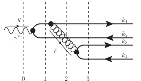
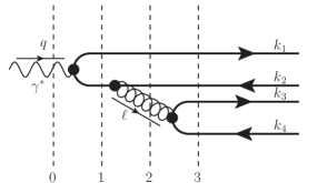
Figure 10: The leading order contribution to the wave function $\psi_{\bar{Q}Q\bar{Q}Q}^{(\gamma)}$ defined in the text. The momenta $k_{i}$ shown in the right-hand side are Fourier conjugates of the coordinates $x_{i}$. It is implied that both diagrams should be supplemented by all possible permutations of final state quarks (see the text for more details).

In leading order over $\alpha_{s}$, the amplitude of the process is given by the two diagrams shown in Figure (10) and depends on the momenta of the 4 quarks in the final state. In what follows we will use the standard notation $\alpha_{i}=k_{i}/q^{+}$ for the fractions of photon momentum carried by each of these fermions, as well as $\boldsymbol{k}_{i\perp}$ for the transverse components of their momenta. We also will use a shorthand notation $\ell=k_{3}+k_{3}$ for the momentum of the virtual gluon connecting different quark lines. For the sake of generality we will assume that the produced quark-antiquark pairs have different flavors, and will use the notations $m_{1}$ for the current mass of the quark line connected to a photon, and $m_{2}$ for the current masses of the quark-antiquark pair produced from the virtual gluon.

Using the rules from Bjorken:1970ah ; Dosch:1996ss , we may obtain for the corresponding amplitude of the subprocess

$$\mathcal{A}_{c_{1}c_{2},c_{3}c_{2}}^{a_{1}a_{2},a_{3}a_{4}} =-\frac{e_{q}g^{2}\,\left(t_{a}\right)_{c_{1}c_{2}}\otimes\left(t_{a}\right)_{c_{3}c_{4}}}{16\,\pi^{2}}\left(\frac{\bar{u}_{a_{1}}\left(k_{1}\right)\hat{\varepsilon}_{\lambda}^{*}(\ell)u_{b}\left(k_{1}+\ell\right)\,\,\bar{u}_{b}\left(q-k_{2}\right)\hat{\varepsilon}_{\gamma}(q)\,v_{a_{2}}\left(k_{2}\right)}{D_{11}D_{12}D_{13}\sqrt{k_{1}^{+}}\sqrt{k_{1}^{+}+\ell^{+}}\sqrt{q^{+}-k_{2}^{+}}\sqrt{k_{2}^{+}}}\right.+$$ (69)

$$-\left.\frac{\bar{u}_{a_{1}}\left(k_{1}\right)\hat{\varepsilon}_{\gamma}(q)v_{b}\left(q-k_{1}\right)\,\,\bar{v}_{b}\left(k_{2}+\ell\right)\hat{\varepsilon}_{\lambda}^{*}(\ell)\,v_{a_{2}}\left(k_{2}\right)}{D_{21}D_{22}D_{23}\sqrt{k_{1}^{+}}\sqrt{q^{+}-k_{1}^{+}}\sqrt{k_{2}^{+}+\ell^{+}}\sqrt{k_{2}^{+}}}\right)\frac{\bar{u}_{a_{3}}\left(k_{3}\right)\hat{\varepsilon}_{\lambda}\left(\ell\right)v_{a_{4}}\left(k_{4}\right)}{\left(k_{3}^{+}+k_{4}^{+}\right)\sqrt{k_{3}^{+}k_{4}^{+}}},$$

where $a_{i}$ and $c_{i}$ are the helicity and color indices of the final state quarks, and $D_{ij}$ are the conventional light-cone denominators (with the first subscript index $i=1,2$ refers to the first and the second diagram in Figure 10 respectively, and the second index $j=1,2,3$ numerates proper cuts shown with dashed vertical lines). Explicitly, these light-cone denominators are given by

$$D_{11} =-\frac{1}{2q^{+}}\left(\frac{\boldsymbol{k}_{2\perp}^{2}+m_{1}^{2}}{\alpha_{2}}+\frac{\left(\boldsymbol{k}_{1\perp}+\boldsymbol{\ell}\right)^{2}+m_{1}^{2}}{\alpha_{1}+z}\right)=-\frac{1}{2q^{+}}\frac{\boldsymbol{k}_{2\perp}^{2}+m_{1}^{2}}{\alpha_{2}\bar{\alpha}_{2}},$$ (70)

$$D_{21} =-\frac{1}{2q^{+}}\left(\frac{\boldsymbol{k}_{1\perp}^{2}+m_{1}^{2}}{\alpha_{1}}+\frac{\left(\boldsymbol{k}_{2\perp}+\boldsymbol{\ell}\right)^{2}+m_{1}^{2}}{\alpha_{2}+z}\right)=-\frac{1}{2q^{+}}\frac{\boldsymbol{k}_{1\perp}^{2}+m_{1}^{2}}{\alpha_{1}\bar{\alpha}_{1}},$$ (71)

$$D_{12} =D_{22}\equiv D_{2}=-\frac{1}{2q^{+}}\left(\frac{\boldsymbol{k}_{1\perp}^{2}+m_{1}^{2}}{\,\alpha_{1}}+\frac{\boldsymbol{k}_{2\perp}^{2}+m_{1}^{2}}{\,\alpha_{2}}+\frac{\boldsymbol{\ell}_{\perp}^{2}}{z}\right)=$$ (72)

$$=-\frac{1}{2q^{+}}\frac{\alpha_{2}\bar{\alpha}_{2}\left(\boldsymbol{k}_{1\perp}+\boldsymbol{k}_{2\perp}\frac{\alpha_{1}}{\bar{\alpha}_{2}}\right)^{2}+\frac{\alpha_{1}}{\bar{\alpha}_{2}}\left(1-\alpha_{1}-\alpha_{2}\right)\boldsymbol{k}_{2\perp}^{2}+m_{1}^{2}\left(\alpha_{1}+\alpha_{2}\right)\left(1-\alpha_{1}-\alpha_{2}\right)}{\alpha_{1}\alpha_{2}\left(1-\alpha_{1}-\alpha_{2}\right)}=$$

$$=-\frac{1}{2q^{+}}\frac{\alpha_{1}\bar{\alpha}_{1}\left(\boldsymbol{k}_{2\perp}+\boldsymbol{k}_{1\perp}\frac{\alpha_{2}}{\bar{\alpha}_{1}}\right)^{2}+\frac{\alpha_{2}}{\bar{\alpha}_{1}}\left(1-\alpha_{1}-\alpha_{2}\right)\boldsymbol{k}_{1\perp}^{2}+m_{1}^{2}\left(\alpha_{1}+\alpha_{2}\right)\left(1-\alpha_{1}-\alpha_{2}\right)}{\alpha_{1}\alpha_{2}\left(1-\alpha_{1}-\alpha_{2}\right)}$$ (73)

$$D_{13} =D_{23}=D_{3}=-\frac{1}{2q^{+}}\left(\sum_{i=1}^{2}\frac{\boldsymbol{k}_{i\perp}^{2}+m_{1}^{2}}{2\,\alpha_{i}}+\sum_{i=3}^{4}\frac{\boldsymbol{k}_{i\perp}^{2}+m_{2}^{2}}{2\,\alpha_{i}}\right)=$$ (74)

$$=D_{12}-\frac{\left(\boldsymbol{k}_{3\perp}\alpha_{4}-\boldsymbol{k}_{4\perp}\alpha_{3}\right)^{2}+m_{2}^{2}\left(\alpha_{3}+\alpha_{4}\right)^{2}}{2q^{+}\alpha_{3}\alpha_{4}\left(\alpha_{3}+\alpha_{4}\right)}=D_{12}-\left(\frac{\alpha_{3}+\alpha_{4}}{\alpha_{3}\alpha_{4}}\right)\frac{\boldsymbol{q}_{34}^{2}+m_{2}^{2}}{2\,q^{+}},$$

$$\boldsymbol{q}_{34} =\frac{\boldsymbol{k}_{3\perp}\alpha_{4}-\boldsymbol{k}_{4\perp}\alpha_{3}}{\alpha_{3}+\alpha_{4}}.$$ (75)

To simplify the structure of the expressions (70-74), we introduced a shorthand notation $\bar{\alpha}_{i}\equiv 1-\alpha_{i},\,\,i=1...4$. The combination of momenta $\boldsymbol{q}_{34}$, defined in (75), represents the relative motion momenta of quarks 3 and 4 (Fourier conjugate of a relative distance $\boldsymbol{r}_{3}-\boldsymbol{r}_{4}$). Technically, the structure of the denominators, up to trivial redefinitions, agrees with the findings of Lappi:2016oup . The expressions in the numerator of (69) can be written out explicitly using the light-cone algebra from Lepage:1980fj ; Brodsky:1997de ; Lappi:2016oup , yielding for the amplitude

$$\mathcal{A}_{c_{1}c_{2},c_{3}c_{4}}^{a_{1}a_{2},a_{3}a_{4}} =\frac{1}{2\pi^{2}\,\left(q^{+}\right)^{2}}\frac{e_{q}\,g^{2}\,\left(t_{a}\right)_{c_{1}c_{2}}\otimes\left(t_{a}\right)_{c_{3}c_{4}}}{\sqrt{\alpha_{1}\alpha_{2}}\left(1-\alpha_{1}-\alpha_{2}\right)\left(\alpha_{3}+\alpha_{4}\right)\,D_{2}\left(\alpha_{1},\boldsymbol{k}_{1};\alpha_{2},\,\boldsymbol{k}_{2}\right)}\times$$ (76)

$$\times\left\{\frac{1}{\boldsymbol{k}_{2\perp}^{2}+m_{1}^{2}}\sqrt{\frac{\alpha_{2}}{\alpha_{1}}}\left[\left(\alpha_{2}\delta_{\gamma,a_{2}}-\bar{\alpha}_{2}\delta_{\gamma,-a_{2}}\right)\delta_{b,-a_{2}}\boldsymbol{k}_{2}\cdot\boldsymbol{\varepsilon}_{\gamma}+\frac{m_{q}}{\sqrt{2}}\,{\rm sign}\left(a_{2}\right)\delta_{\gamma,a_{2}}\delta_{b,\,a_{2}}\right]\right.\times$$

$$\times\left[\left(\bar{\alpha}_{2}\delta_{\lambda,\,a_{1}}+\alpha_{1}\delta_{\lambda,-a_{1}}\right)\delta_{a_{1},b}\boldsymbol{q}_{1}\cdot\boldsymbol{\varepsilon}_{\lambda}^{*}+\frac{m_{q}}{\sqrt{2}}\frac{\left(1-\alpha_{1}-\alpha_{2}\right)^{2}}{1-\alpha_{2}}\,{\rm sign}\left(-a_{1}\right)\delta_{\lambda,-a_{1}}\delta_{a_{1},-b}\right]$$

$$-\frac{1}{\boldsymbol{k}_{1\perp}^{2}+m_{1}^{2}}\sqrt{\frac{\alpha_{1}}{\alpha_{2}}}\left[\left(\alpha_{1}\delta_{\gamma,a_{1}}-\bar{\alpha}_{1}\delta_{\gamma,-a_{1}}\right)\delta_{b,-a_{1}}\boldsymbol{k}_{1}\cdot\boldsymbol{\varepsilon}_{\gamma}+\frac{m_{q}}{\sqrt{2}}\,{\rm sign}\left(a_{1}\right)\delta_{\gamma,a_{1}}\delta_{a_{1},b}\right]\times$$

$$\times\left.\left[\left(\bar{\alpha}_{1}\delta_{\lambda,\,a_{2}}+\alpha_{2}\delta_{\lambda,-a_{2}}\right)\delta_{a_{2},b}\boldsymbol{q}_{2}\cdot\boldsymbol{\varepsilon}_{\lambda}^{*}+\frac{m_{q}}{\sqrt{2}}\frac{\left(1-\alpha_{1}-\alpha_{2}\right)^{2}}{1-\alpha_{1}}\,{\rm sign}\left(-a_{2}\right)\delta_{\lambda,-a_{2}}\delta_{a_{2},-b}\right]\right\}\times$$

$$\times\frac{\frac{2\left(\alpha_{3}+\alpha_{4}\right)}{\alpha_{3}\alpha_{4}}\left[\left(\frac{\alpha_{3}}{\alpha_{3}+\alpha_{4}}\delta_{\lambda,-a_{3}}-\frac{\alpha_{4}}{\alpha_{3}+\alpha_{4}}\delta_{\lambda,a_{3}}\right)\delta_{a_{3},-a_{4}}\boldsymbol{q}_{34}\cdot\boldsymbol{\varepsilon}_{-\lambda}+\frac{m_{q}}{\sqrt{2}}\,{\rm sign}(a_{3})\delta_{\lambda,a_{3}}\delta_{a_{3},a_{4}}\right]}{D_{2}\left(\alpha_{1},\boldsymbol{k}_{1};\alpha_{2},\,\boldsymbol{k}_{2}\right)-\frac{\boldsymbol{q}_{34}^{2}+m_{2}^{2}}{2q^{+}}\left(\frac{\alpha_{3}+\alpha_{4}}{\alpha_{3}\alpha_{4}}\right)}$$

where the momenta $\boldsymbol{q}_{i}$ are defined as

$$\boldsymbol{q}_{1}=-\left(\boldsymbol{k}_{1}+\frac{\alpha_{1}}{1-\alpha_{2}}\boldsymbol{k}_{2}\right),\qquad\boldsymbol{q}_{2}=-\left(\boldsymbol{k}_{2}+\frac{\alpha_{2}}{1-\alpha_{1}}\boldsymbol{k}_{1}\right).$$ (77)

We may observe that the amplitude (76) is antisymmetric with respect to permutation of the momenta and helicities of the first two quarks, $\left(\alpha_{1},\,\boldsymbol{k}_{1},\,a_{1}\right)\leftrightarrow\left(\alpha_{2},\,\boldsymbol{k}_{2},\,a_{2}\right)$, and symmetric with respect to permutation of the the momenta and helicities of the 3rd and 4th quarks, $\left(\alpha_{3},\,\boldsymbol{k}_{3},\,a_{3}\right)\leftrightarrow\left(\alpha_{4},\,\boldsymbol{k}_{4},\,a_{4}\right)$. This symmetry simply reflects that the amplitude (76) was evaluated as a sum of the left and the right diagrams in Figure 10, which can be related by charge conjugation. This symmetry allows to simplify some evaluations.

For evaluations in the dipole framework we need to rewrite the amplitude in configuration space, making a Fourier transformation over the transverse components,

$$\psi_{\bar{Q}Q\bar{Q}Q}^{(\gamma)}\left(\left\{\alpha_{i},\,\boldsymbol{x}_{i}\right\}\right)=\int\left(\prod_{i=1}^{4}\frac{d^{2}k_{i}}{\left(2\pi\right)^{2}}e^{i\boldsymbol{k}_{i}\cdot\boldsymbol{x}_{i}}\right)(2\pi)^{2}\delta^{2}\left(\sum\boldsymbol{k}_{i}\right)\mathcal{A}_{c_{1}c_{2},c_{3}c_{4}}^{a_{1}a_{2},a_{3}a_{4}}\left(\left\{\alpha_{i},\,\boldsymbol{k}_{i}\right\}\right)$$ (78)

In view of momentum conservation (55), the wave function $\psi_{\bar{Q}Q\bar{Q}Q}^{(\gamma)}$ will be invariant with respect to global shifts

$$\boldsymbol{x}_{i}\to\boldsymbol{x}_{i}+\boldsymbol{a}_{i},\quad\boldsymbol{a}_{i}={\rm const},$$ (79)

i.e. should depend only on relative distances between quarks $\left|\boldsymbol{x}_{i}-\boldsymbol{x}_{j}\right|$. After straightforward evaluation of the integrals and algebraic simplifications it is possible to reduce (78) to the form

$$\psi_{\bar{Q}Q\bar{Q}Q}^{(\gamma)}\left(\left\{\alpha_{i},\,\boldsymbol{x}_{i}\right\}\right)=A\left(\left\{\alpha_{i},\,\boldsymbol{x}_{i}\right\}\right)+B\left(\left\{\alpha_{i},\,\boldsymbol{x}_{i}\right\}\right).$$ (80)

where

$$A\left(\left\{\alpha_{i},\,\boldsymbol{r}_{i}\right\}\right) =-\frac{2e_{q}\alpha_{s}\left(m_{Q}\right)\,\left(t_{a}\right)_{c_{1}c_{2}}\otimes\left(t_{a}\right)_{c_{3}c_{4}}}{\pi^{3}\left(1-\alpha_{1}-\alpha_{2}\right)^{2}\sqrt{\alpha_{1}\alpha_{2}}\,}\int\frac{q_{1}dq_{1}\,k_{2}dk_{2}}{\frac{\bar{\alpha}_{2}q_{1}^{2}}{\alpha_{1}\left(1-\alpha_{1}-\alpha_{2}\right)}+\frac{m_{1}^{2}\left(\alpha_{1}+\alpha_{2}\right)}{\alpha_{1}\alpha_{2}}+\frac{k_{2}^{2}}{\alpha_{2}\bar{\alpha}_{2}}}\times$$ (81)

$$\times\frac{1}{k_{2}^{2}+m_{1}^{2}}\sqrt{\frac{\alpha_{2}}{\alpha_{1}}}\left[\left(\alpha_{2}\delta_{\gamma,a_{2}}-\bar{\alpha}_{2}\delta_{\gamma,-a_{2}}\right)\left(\bar{\alpha}_{2}\delta_{\lambda,\,a_{1}}+\alpha_{1}\delta_{\lambda,-a_{1}}\right)\delta_{a_{1},-a_{2}}\times\right.$$

$$\times\left(\boldsymbol{n}_{2,134}\cdot\boldsymbol{\varepsilon}_{\gamma}\right)\left(\boldsymbol{n}_{1,34}\cdot\boldsymbol{\varepsilon}_{\lambda}^{*}\right)k_{2}\,J_{1}\left(k_{2}\left|\boldsymbol{x}_{2}-\boldsymbol{b}_{134}\right|\right)q_{1}J_{1}\left(q_{1}\left|\boldsymbol{x}_{1}-\boldsymbol{b}_{34}\right|\right)+$$

$$+\frac{m_{q}^{2}}{2}\,\delta_{\lambda,-a_{1}}\delta_{\gamma,a_{2}}\delta_{a_{1},-a_{2}}J_{0}\left(k_{2}\left|\boldsymbol{x}_{2}-\boldsymbol{b}_{134}\right|\right)J_{0}\left(q_{1}\left|\boldsymbol{x}_{1}-\boldsymbol{b}_{34}\right|\right)\frac{\left(1-\alpha_{1}-\alpha_{2}\right)^{2}}{1-\alpha_{2}}$$

$$-\frac{im_{q}}{\sqrt{2}}\,{\rm sign}\left(a_{2}\right)\delta_{\gamma,a_{2}}\delta_{a_{1},a_{2}}\left(\bar{\alpha}_{2}\delta_{\lambda,\,a_{1}}+\alpha_{1}\delta_{\lambda,-a_{1}}\right)\times$$

$$\times\boldsymbol{n}_{1,34}\cdot\boldsymbol{\varepsilon}_{\lambda}^{*}q_{1}J_{1}\left(q_{1}\left|\boldsymbol{x}_{1}-\boldsymbol{b}_{34}\right|\right)J_{0}\left(k_{2}\left|\boldsymbol{x}_{2}-\boldsymbol{b}_{134}\right|\right)$$

$$-\frac{im_{q}}{\sqrt{2}}{\rm sign}\left(a_{1}\right)\delta_{\lambda,-a_{1}}\left(\alpha_{2}\delta_{\gamma,a_{2}}-\bar{\alpha}_{2}\delta_{\gamma,-a_{2}}\right)\delta_{a_{1},a_{2}}\frac{\left(1-\alpha_{1}-\alpha_{2}\right)^{2}}{1-\alpha_{2}}\times$$

$$\times\left.\left(\boldsymbol{n}_{2,134}\cdot\boldsymbol{\varepsilon}_{\gamma}\right)k_{2}\,J_{1}\left(k_{2}\left|\boldsymbol{x}_{2}-\boldsymbol{b}_{134}\right|\right)J_{0}\left(q_{1}\left|\boldsymbol{x}_{1}-\boldsymbol{b}_{34}\right|\right)\right]\times$$

$$\times\Psi_{a_{3},a_{4}}^{-\lambda}\left(\frac{\alpha_{3}}{\alpha_{3}+\alpha_{4}},\,\boldsymbol{r}_{34},\,m_{2},\,\sqrt{m_{2}^{2}+\frac{\alpha_{3}\alpha_{4}}{\alpha_{3}+\alpha_{4}}\left[\frac{\bar{\alpha}_{2}q_{1}^{2}}{\alpha_{1}\left(1-\alpha_{1}-\alpha_{2}\right)}+\frac{m_{1}^{2}\left(\alpha_{1}+\alpha_{2}\right)}{\alpha_{1}\alpha_{2}}+\frac{k_{2}^{2}}{\alpha_{2}\bar{\alpha}_{2}}\right]}\right)$$

and

$$B\left(\alpha_{1},\,\boldsymbol{x}_{1},\,\alpha_{2},\,\boldsymbol{x}_{2},\,\alpha_{3},\,\boldsymbol{x}_{3},\,\alpha_{4},\,\boldsymbol{x}_{4}\right)=-A\left(\alpha_{2},\,\boldsymbol{x}_{2},\,\alpha_{1},\,\boldsymbol{x}_{1},\,\alpha_{4},\,\boldsymbol{x}_{4},\,\alpha_{3},\,\boldsymbol{x}_{3}\right).$$

The variable $\boldsymbol{b}_{j_{1}...j_{n}}$ corresponds to the position of the center of mass of $n$ partons $j_{1},\,...j_{n}$ and was defined earlier in (24). The variables $\boldsymbol{n}_{i,j_{1}...j_{n}}=\left(\boldsymbol{x}_{i}-\boldsymbol{b}_{j_{1}...j_{n}}\right)/\left|\boldsymbol{x}_{i}-\boldsymbol{b}_{j_{1}...j_{n}}\right|$ are unit vectors pointing from quark $i$ towards the center-of-mass of a system of quarks $j_{1}...j_{n}$. It is not possible to do the remaining integrals over $q_{1},\,k_{2}$ analytically, nor present the wave function (81) as a convolution of simpler “elementary” wave functions from Section B.1.. Technically, this happens because in the language of traditional Feynman diagrams the intermediate (virtual) partons are offshell, and the integration over $q_{1},k_{2}$ can be rewritten via integrals over virtualities of intermediate particles. Nevertheless, the structure of the coordinate dependence of $\psi_{\gamma\to\bar{Q}Q\bar{Q}Q}\left(\left\{\alpha_{i},\,\boldsymbol{r}_{i}\right\}\right)$ can still be understood using the simple rules suggested in Section B.1. Indeed, in the eikonal picture the transverse coordinates of all partons are frozen. The tree-like structure of the leading order diagrams 1, 2, in Fig. 10 and the iterative evaluation of the coordinate of the center of mass of two partons $\boldsymbol{b}_{ij}=\left(\alpha_{i}\boldsymbol{r}_{i}+\alpha_{j}\boldsymbol{r}_{j}\right)/\left(\alpha_{i}+\alpha_{j}\right)$ allows to reconstruct the transverse coordinates of all intermediate partons, as shown in Figure 11. The variables $\boldsymbol{r}_{1}-\boldsymbol{b}_{34}$ and $\boldsymbol{r}_{2}-\boldsymbol{b}_{34}$ have the physical meaning of the relative distance between the recoil quark or antiquark and the emitted gluon. Similarly, the variables $\boldsymbol{r}_{1}-\boldsymbol{b}_{234}$ and $\boldsymbol{r}_{2}-\boldsymbol{b}_{134}$ can be interpreted as the size of the $\bar{Q}Q$ pair produced right after splitting of the incident photon. These simple rules allow for the construction of the heavy $\bar{Q}Q\bar{Q}Q$ production amplitude in the gluonic field of the target.

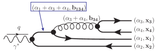
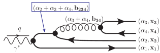
Figure 11: Graphical illustration of the transverse momentum dependence of the wave function $\psi_{\gamma\to\bar{Q}Q\bar{Q}Q}\left(\left\{\alpha_{i},\,\boldsymbol{r}_{i}\right\}\right)$. The letters $\boldsymbol{b}_{ij}$ and $\boldsymbol{b}_{ijk}$ stand for the center of mass position of the partons $ij$ or $ijk$. See the text for more details.

The wave function $\psi_{\bar{Q}Q\bar{Q}Q}^{(\gamma)}\left(\left\{\alpha_{i},\,\boldsymbol{r}_{i}\right\}\right)$ has a few singularities which require special attention in order to guarantee that the amplitudes of the physical processes remain finite. For the meson pair production, the choice of the quarkonia wave functions (28-31), which vanish rapidly near the endpoints is sufficient in order to guarantee finiteness of the amplitudes (22-23).

B.2.2 Instantaneous contributions

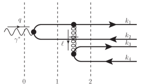
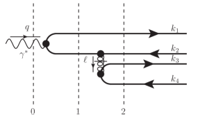
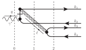
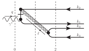
Figure 12: The instantaneous contributions to the wave function $\psi_{\bar{Q}Q\bar{Q}Q}^{(\gamma)}$ defined in the text. The upper and lower rows correspond to instantaneous gluons and quarks respectively. The vertical dashed lines denote light-cone denominators. The momenta $k_{i}$ shown in the right-hand side are Fourier conjugates of the coordinates $x_{i}$. In what follows we will refer to the diagrams in the first row as A1, B1, and the diagrams in the second row as A2, B2, respectively.

According to canonical rules of the standard light–cone perturbation theory Lepage:1980fj ; Brodsky:1997de , the evaluations from the previous section should be supplemented by the instantaneous contributions of virtual partons. The propagators of the instantaneous offshell quarks and gluons with momentum $k$ are given by

$$S_{({\rm inst)}}(k)=\frac{\gamma^{+}}{2k^{+}}\equiv\frac{\left(n\cdot\gamma\right)}{2\left(k\cdot n\right)},\quad\Pi_{({\rm inst})}^{\mu\nu}=\frac{n_{\mu}n_{\nu}}{\left(k^{+}\right)^{2}}$$ (82)

where $n^{\mu}$ is the light-cone vector in minus-direction. The results for the instantaneous contributions of gluons are quite straightforward to get, essentially repeating the evaluations from the previous subsection. Since $\gamma_{+}\gamma_{+}=0$, there is no diagrams with two instantaneous propagators (quark and gluon) connected to the same vertex. The numerators of amplitudes with instantaneous propagators have simple structure in view of identities Lepage:1980fj ; Brodsky:1997de ; Lappi:2016oup $\bar{u}_{h_{f}}\left(p_{1}\right)\gamma_{+}u_{h_{i}}\left(p_{2}\right)=2\sqrt{p_{1}^{+}p_{2}^{+}}\delta_{h_{f},h_{i}}$and $\bar{u}_{h}\left(p_{1}\right)\gamma_{+}v_{\bar{h}}\left(p_{2}\right)=2\sqrt{p_{1}^{+}p_{2}^{+}}\delta_{h,\,-\bar{h}}$. The final result of the evaluation is

$$\psi_{\bar{Q}Q\bar{Q}Q}^{(\gamma)}\left(\left\{\alpha_{i},\,\boldsymbol{r}_{i}\right\}\right) =A_{g}\left(\left\{\alpha_{i},\,\boldsymbol{r}_{i}\right\}\right)+B_{g}\left(\left\{\alpha_{i},\,\boldsymbol{r}_{i}\right\}\right)+$$ (83)

$$+A_{q}\left(\left\{\alpha_{i},\,\boldsymbol{r}_{i}\right\}\right)+B_{q}\left(\left\{\alpha_{i},\,\boldsymbol{r}_{i}\right\}\right),$$

where the subscript indices $q,g$ in the right-hand side denote the parton propagator, which should be taken instantaneous ($q$ for quark, $g$ for gluon), and

$$A_{g}\left(\left\{\alpha_{i},\,\boldsymbol{r}_{i}\right\}\right) =-\frac{e_{q}\alpha_{s}(m_{Q})\,\left(t_{a}\right)_{c_{1}c_{2}}\otimes\left(t_{a}\right)_{c_{3}c_{4}}}{\pi^{4}\left(1-\alpha_{1}-\alpha_{2}\right)^{3}\,}\int q_{1}dq_{1}\,k_{2}dk_{2}J_{0}\left(q_{1}\left|\boldsymbol{r}_{1}-\boldsymbol{b}_{34}\right|\right)\times$$ (84)

$$\times\frac{1}{\boldsymbol{k}_{2\perp}^{2}+m_{1}^{2}}\left[\left(\alpha_{2}\delta_{\gamma,a_{1}}-\bar{\alpha}_{2}\delta_{a_{1},-\gamma}\right)\delta_{a_{1},-a_{2}}i\boldsymbol{n}_{2,134}\cdot\boldsymbol{\varepsilon}_{\gamma}k_{2}J_{1}\left(k_{2}\left|\boldsymbol{r}_{2}-\boldsymbol{b}_{134}\right|\right)\right.$$

$$\left.+\frac{m_{q}}{\sqrt{2}}\,{\rm sign}\left(a_{1}\right)\delta_{\gamma,a_{1}}\delta_{a_{1},a_{2}}J_{0}\left(k_{2}\left|\boldsymbol{r}_{2}-\boldsymbol{b}_{134}\right|\right)\right]\alpha_{3}\alpha_{4}\delta_{a_{3},-a_{4}}K_{0}\left(a_{34}\,\boldsymbol{r}_{34}\right).$$

$$A_{q}\left(\left\{\alpha_{i},\,\boldsymbol{r}_{i}\right\}\right) =-\frac{e_{q}\alpha_{s}\left(m_{q}\right)\,\left(t_{a}\right)_{c_{1}c_{2}}\otimes\left(t_{a}\right)_{c_{3}c_{4}}}{2\pi^{4}\left(1-\alpha_{1}-\alpha_{2}\right)^{2}\bar{\alpha}_{2}}\delta_{a_{1},-a_{2}}\delta_{\gamma,-a_{1}}\int q_{1}dq_{1}\,k_{2}dk_{2}\frac{J_{0}\left(q_{1}\left|\boldsymbol{r}_{1}-\boldsymbol{b}_{34}\right|\right)J_{0}\left(k_{2}\left|\boldsymbol{r}_{2}-\boldsymbol{b}_{134}\right|\right)}{D_{2}\left(\alpha_{1},\boldsymbol{k}_{1};\alpha_{2},\,\boldsymbol{k}_{2}\right)}\times$$ (85)

$$\times\left[-\left(\alpha_{3}\delta_{-\gamma,a_{3}}-\alpha_{4}\delta_{\gamma,a_{3}}\right)\delta_{a_{3},-a_{4}}i\boldsymbol{\varepsilon}_{\gamma}\cdot\boldsymbol{n}_{34}a_{34}K_{1}\left(a_{34}\,\boldsymbol{r}_{34}\right)-\frac{m_{q}(\alpha_{3}+\alpha_{4})}{\sqrt{2}}\,{\rm sign}(a_{3})\delta_{\gamma,-a_{3}}\delta_{a_{3},a_{4}}K_{0}\left(a_{34}\,\boldsymbol{r}_{34}\right)\right]$$

$$a_{34}\left(q_{1},\,k_{2}\right)\equiv\sqrt{m_{2}^{2}+\frac{\alpha_{3}\alpha_{4}}{\alpha_{3}+\alpha_{4}}\left[\frac{\bar{\alpha}_{2}q_{1}^{2}}{\alpha_{1}\left(1-\alpha_{1}-\alpha_{2}\right)}+\frac{m_{1}^{2}\left(\alpha_{1}+\alpha_{2}\right)}{\alpha_{1}\alpha_{2}}+\frac{k_{2}^{2}}{\alpha_{2}\bar{\alpha}_{2}}\right]}$$ (86)

and the functions $B_{q},\,B_{g}$ can be obtained from $A_{q},A_{g}$ using

$$B_{i}\left(\alpha_{1},\,\boldsymbol{x}_{1},\,\alpha_{2},\,\boldsymbol{x}_{2},\,\alpha_{3},\,\boldsymbol{x}_{3},\,\alpha_{4},\,\boldsymbol{x}_{4}\right)=-A_{i}\left(\alpha_{2},\,\boldsymbol{x}_{2},\,\alpha_{1},\,\boldsymbol{x}_{1},\,\alpha_{4},\,\boldsymbol{x}_{4},\,\alpha_{3},\,\boldsymbol{x}_{3}\right),\quad i=q,g.$$ (87)

Appendix C Scattering amplitudes in the eikonal approximation

As was discussed in Section A, in configuration space the interaction of the target with heavy quarks reduces to a mere multiplication by the factor $\pm\gamma\left(\boldsymbol{x}_{\perp}\right)$. For evaluation of the scattering amplitude it is very instructive to use the light-cone evolution picture of the process, as shown in Figure 10, tacitly assuming that the cuts (vertical dashed lines) in that figure separate different successive stages of the scattering process.

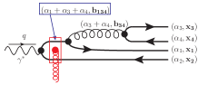
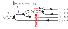
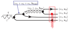
Figure 13: Schematic illustration of the diagrams which contribute to a $\gamma\to\bar{Q}Q\bar{Q}Q$ subprocess, via single-gluon exchange in $t$-channel. For the sake of simplicity we omitted a proton blob in the lower part. The square box with gluon connected in the middle stands for a coupling of a dipole (sum of the couplings to all partons which pass through the block, $\sim\sum(\pm)\gamma(\boldsymbol{x}_{i})t_{a}$). The center-of-mass $\boldsymbol{b}_{i_{1}...i_{n}}$ of a system of partons $i_{1}...i_{n}$ is defined in (24). In all plots it is implied the inclusion of diagrams which can be obtained by inversion of heavy quark lines (“charge conjugation”).

We will start assuming first a single-gluon interaction with high-energy partons. The colorless photon creates a pair of quark and antiquarks with transverse coordinates $(\boldsymbol{b}_{134}$,$\boldsymbol{x}_{2})$ or $(\boldsymbol{x}_{1},\,\boldsymbol{b}_{234}$$)$ respectively, as shown in Figure13. The eikonal interaction can occur at any of the three stages of the process, so the Born amplitude of such process includes a sum of contributions due to interactions at all stages,

$$\mathcal{A}=\mathcal{A}_{1}+\mathcal{A}_{2}+\mathcal{A}_{3},$$ (88)

where the corresponding contributions $\mathcal{A}_{1,2,3}$ are given by

$$\mathcal{A}_{1} =\psi_{\bar{Q}Q\bar{Q}Q}^{(\gamma)}\left(\alpha_{1},\boldsymbol{x}_{1};\,\alpha_{2},\,\boldsymbol{x}_{2};\,\alpha_{3},\,\boldsymbol{x}_{3};\,\alpha_{4},\,\boldsymbol{x}_{4};\,q\right)\times$$ (89)

$$\times\sum_{acd}\left[\gamma_{c}\left(\boldsymbol{b}_{134}\right)-\gamma_{c}\left(\boldsymbol{x}_{2}\right)\right]\left(\frac{if_{acd}+d_{acd}}{2}\right)\left(t_{d}\right)_{c_{1}c_{2}}\left(t_{a}\right)_{c_{3}c_{4}}$$

$$-\left(1\leftrightarrow 2,\,\,3\leftrightarrow 4\right),$$

$$\mathcal{A}_{2} =\psi_{\bar{Q}Q\bar{Q}Q}^{(\gamma)}\left(\alpha_{1},\boldsymbol{x}_{1};\,\alpha_{2},\,\boldsymbol{x}_{2};\,\alpha_{3},\,\boldsymbol{x}_{3};\,\alpha_{4},\,\boldsymbol{x}_{4};\,q\right)\times$$ (90)

$$\times\left\{\sum_{acd}\left[\gamma_{c}\left(\boldsymbol{x}_{1}\right)+\gamma_{c}\left(\boldsymbol{x}_{2}\right)-2\gamma_{c}\left(\boldsymbol{x}_{34}\right)\right]\left(\frac{if_{acd}}{2}\right)\left(t_{d}\right)_{c_{1}c_{2}}\left(t_{a}\right)_{c_{3}c_{4}}\right.+$$

$$+\sum_{acd}\left[\gamma_{c}\left(\boldsymbol{x}_{1}\right)-\gamma_{c}\left(\boldsymbol{x}_{2}\right)\right]\left(\frac{d_{acd}}{2}\right)\left(t_{d}\right)_{c_{1}c_{2}}\left(t_{a}\right)_{c_{3}c_{4}}+$$

$$+\left.\sum_{acd}\left[\gamma_{c}\left(\boldsymbol{x}_{1}\right)-\gamma_{c}\left(\boldsymbol{x}_{2}\right)\right]\delta_{c_{1}c_{2}}\left(t_{c}\right)_{c_{3}c_{4}}\right\}$$

$$-\left(1\leftrightarrow 2,\,\,3\leftrightarrow 4\right),$$

$$\mathcal{A}_{3} =\psi_{\bar{Q}Q\bar{Q}Q}^{(\gamma)}\left(\alpha_{1},\boldsymbol{x}_{1};\,\alpha_{2},\,\boldsymbol{x}_{2};\,\alpha_{3},\,\boldsymbol{x}_{3};\,\alpha_{4},\,\boldsymbol{x}_{4};\,q\right)\times$$ (91)

$$\times\left\{\sum_{acd}\left[\gamma_{c}\left(\boldsymbol{x}_{1}\right)+\gamma_{c}\left(\boldsymbol{x}_{2}\right)-\gamma_{c}\left(\boldsymbol{x}_{3}\right)-\gamma_{c}\left(\boldsymbol{x}_{4}\right)\right]\left(\frac{if_{cad}}{2}\right)\left(t_{d}\right)_{c_{1}c_{2}}\left(t_{a}\right)_{c_{3}c_{4}}\right.+$$

$$+\left.\sum_{acd}\left[\gamma_{c}\left(\boldsymbol{x}_{1}\right)-\gamma_{c}\left(\boldsymbol{x}_{2}\right)+\gamma_{c}\left(\boldsymbol{x}_{3}\right)-\gamma_{c}\left(\boldsymbol{x}_{4}\right)\right]\left(\frac{d_{acd}}{2}\right)\left(t_{d}\right)_{c_{1}c_{2}}\left(t_{a}\right)_{c_{3}c_{4}}\right\}$$

$$-\left(1\leftrightarrow 2,\,\,3\leftrightarrow 4\right),$$

We may observe that all factors $\gamma_{c}(\boldsymbol{x}_{i})$ always appear in combination $\gamma_{c}(\boldsymbol{x}_{i})-\gamma_{c}(\boldsymbol{x}_{j})$, which guarantees that in the heavy quark mass limit, when the distances between the quarks are small, the corresponding amplitude is suppressed at least as $\sim 1/m_{Q}$. The three-gluon coupling $\sim\gamma\left(\boldsymbol{x}_{34}\right)$ always appears in combination $\left[\gamma_{c}\left(\boldsymbol{x}_{1}\right)+\gamma_{c}\left(\boldsymbol{x}_{2}\right)-2\gamma_{c}\left(\boldsymbol{x}_{34}\right)\right],$ in agreement with the earlier findings of Kopeliovich:2002yv .

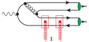
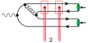
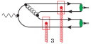
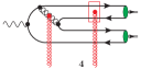
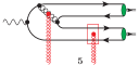
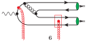
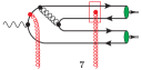
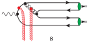
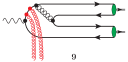
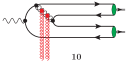
Figure 14: Schematic illustration of the diagrams which contribute to meson pair production. For the sake of simplicity we approximated a pomeron with a pair of $t$-channel gluons, and omitted all possible gluon exchanges between them (as well as a proton blob in the lower part). The square box with gluon connected in the middle stands for a dipole coupling (sum of the couplings of a quark and antiquark which pass through the block, $\sim\left(\gamma(\boldsymbol{x}_{Q})-\gamma(\boldsymbol{x}_{\bar{Q}})\right)t_{a}$). In all plots it is implied the inclusion of diagrams which can be obtained by inversion of the heavy quark lines (“charge conjugation”).

For the case of two gluon exchanges, we may repeat the same evaluations, taking into account the set of diagrams shown in Figure 14. The final result of this evaluation is

$$\mathcal{A} =\psi_{\bar{Q}Q\bar{Q}Q}^{(\gamma)}\left(\alpha_{1},\boldsymbol{x}_{1};\,\alpha_{2},\,\boldsymbol{x}_{2};\,\alpha_{3},\,\boldsymbol{x}_{3};\,\alpha_{4},\,\boldsymbol{x}_{4};\,q\right)\times$$ (92)

$$\times\left\{\mathcal{C}_{1}\left[\left(\gamma\left(\boldsymbol{x}_{1}\right)-\gamma\left(\boldsymbol{x}_{4}\right)\right)^{2}+\left(\gamma\left(\boldsymbol{x}_{3}\right)-\gamma\left(\boldsymbol{x}_{2}\right)\right)^{2}\right]+\right.$$ (93)

$$+2\mathcal{C}_{2}\left(\gamma\left(\boldsymbol{x}_{1}\right)-\gamma\left(\boldsymbol{x}_{4}\right)\right)\left(\gamma\left(\boldsymbol{x}_{3}\right)-\gamma\left(\boldsymbol{x}_{2}\right)\right)-$$

$$+\mathcal{C}_{3}\left(\gamma\left(\boldsymbol{x}_{1}\right)+\gamma\left(\boldsymbol{x}_{2}\right)-2\gamma\left(\boldsymbol{x}_{34}\right)\right)\left(\gamma\left(\boldsymbol{x}_{1}\right)+\gamma\left(\boldsymbol{x}_{2}\right)-\gamma\left(\boldsymbol{x}_{3}\right)-\gamma\left(\boldsymbol{x}_{4}\right)\right)$$

$$+\mathcal{C}_{1}\left(\gamma\left(\boldsymbol{b}_{134}\right)-\gamma\left(\boldsymbol{x}_{2}\right)\right)\left(\gamma\left(\boldsymbol{x}_{3}\right)-\gamma\left(\boldsymbol{x}_{2}\right)\right)+$$

$$+\mathcal{C}_{2}\left(\gamma\left(\boldsymbol{b}_{134}\right)-\gamma\left(\boldsymbol{x}_{2}\right)\right)\left(\gamma\left(\boldsymbol{x}_{1}\right)-\gamma\left(\boldsymbol{x}_{4}\right)\right)+$$

$$-\mathcal{C}_{3}\left(\gamma\left(\boldsymbol{b}_{134}\right)-\gamma\left(\boldsymbol{x}_{2}\right)\right)\left(\gamma\left(\boldsymbol{x}_{1}\right)+\gamma\left(\boldsymbol{x}_{2}\right)-2\gamma\left(\boldsymbol{x}_{34}\right)\right)+$$

$$+\left.\mathcal{C}_{1}\left(\gamma\left(\boldsymbol{b}_{134}\right)-\gamma\left(\boldsymbol{x}_{2}\right)\right)^{2}+\mathcal{C}_{4}\left(\gamma\left(\boldsymbol{x}_{1}\right)+\gamma\left(\boldsymbol{x}_{2}\right)-2\gamma\left(\boldsymbol{x}_{34}\right)\right)^{2}\right\}$$

where the color factors $\mathcal{C}_{1,2,3}$ were defined earlier in Section II.2, in the text under Eq. (23). With the help of (43, 45) it is possible to rewrite the amplitude (92) as

$$\mathcal{A} =\psi_{\bar{Q}Q\bar{Q}Q}^{(\gamma)}\left(\alpha_{1},\boldsymbol{x}_{1};\,\alpha_{2},\,\boldsymbol{x}_{2};\,\alpha_{3},\,\boldsymbol{x}_{3};\,\alpha_{4},\,\boldsymbol{x}_{4};\,q\right)\times$$ (94)

$$\left\{-2\mathcal{C}_{1}\left[N\left(x,\,\boldsymbol{r}_{14},\,\boldsymbol{b}_{14}\right)+N\left(x,\,\boldsymbol{r}_{23},\,\boldsymbol{b}_{23}\right)\right]+\right.$$

$$+2\mathcal{C}_{2}\left[N\left(x,\,\boldsymbol{r}_{34},\,\boldsymbol{b}_{34}\right)+N\left(x,\,\boldsymbol{r}_{12},\,\boldsymbol{b}_{12}\right)\right.\left.-N\left(x,\,\boldsymbol{r}_{13},\,\boldsymbol{b}_{13}\right)-N\left(x,\,\boldsymbol{r}_{24},\,\boldsymbol{b}_{24}\right)\right]$$

$$+\mathcal{C}_{3}\left[-2N\left(x,\boldsymbol{r}_{12},\boldsymbol{b}_{12}\right)+N\left(x,\boldsymbol{r}_{13},\boldsymbol{b}_{13}\right)+N\left(x,\boldsymbol{r}_{14},\boldsymbol{b}_{14}\right)+N\left(x,\boldsymbol{r}_{23},\boldsymbol{b}_{23}\right)+N\left(x,\boldsymbol{r}_{24},\boldsymbol{b}_{24}\right)\right.$$

$$\left.+2N\left(x,\boldsymbol{\boldsymbol{r}}_{1,34},\boldsymbol{b}_{134}\right)+2N\left(x,\boldsymbol{\boldsymbol{r}}_{2,34},\boldsymbol{b}_{234}\right)-2N\left(x,\boldsymbol{\boldsymbol{r}}_{3,34},\boldsymbol{b}_{334}\right)-2N\left(x,\boldsymbol{\boldsymbol{r}}_{4,34},\boldsymbol{b}_{344}\right)\right]$$

$$+\mathcal{C}_{1}\left[N\left(x,\,\boldsymbol{r}_{2,134},\boldsymbol{b}_{1234}\right)+N\left(x,\,\boldsymbol{r}_{23},\,\boldsymbol{b}_{23}\right)-N\left(x,\,\boldsymbol{r}_{3,134},\,\boldsymbol{b}_{1334}\right)\right]$$

$$+\mathcal{C}_{2}\left[N\left(x,\,\boldsymbol{r}_{4,134},\,\boldsymbol{b}_{1344}\right)+N\left(x,\,\boldsymbol{r}_{12},\,\boldsymbol{b}_{12}\right)-N\left(x,\,\boldsymbol{r}_{1,134},\,\boldsymbol{b}_{1,134}\right)-N\left(x,\,\boldsymbol{r}_{24},\,\boldsymbol{b}_{24}\right)\right]$$

$$-\mathcal{C}_{3}\left[-N\left(x,\boldsymbol{r}_{1,134},\boldsymbol{b}_{1134}\right)-N\left(x,\boldsymbol{r}_{2,134},\boldsymbol{b}_{1234}\right)+N\left(x,\boldsymbol{r}_{12},\boldsymbol{b}_{12}\right)\right.$$

$$\,\,\,\,\,\left.+2N\left(x,\boldsymbol{r}_{34,134},\boldsymbol{b}_{34,134}\right)-2N\left(x,\boldsymbol{r}_{2,34},\boldsymbol{b}_{234}\right)\right]+\mathcal{C}_{1}N\left(x,\,\boldsymbol{r}_{2,134},\boldsymbol{b}_{1234}\right)$$

$$+\left.\mathcal{C}_{4}\left[2N\left(x,\,\boldsymbol{r}_{1,34},\,\boldsymbol{b}_{134}\right)+2N\left(x,\,\boldsymbol{r}_{2,34},\,\boldsymbol{b}_{234}\right)-N\left(x,\,\boldsymbol{r}_{12},\,\boldsymbol{b}_{12}\right)\right]\right\}$$

where

$$\boldsymbol{r}_{1,34} =\boldsymbol{r}_{1}-\frac{\alpha_{3}\boldsymbol{r}_{3}+\alpha_{4}\boldsymbol{r}_{4}}{\alpha_{3}+\alpha_{4}}=\frac{\alpha_{3}\boldsymbol{r}_{13}+\alpha_{4}\boldsymbol{r}_{14}}{\alpha_{3}+\alpha_{4}},$$ (95)

$$\boldsymbol{r}_{2,34} =\frac{\alpha_{3}\boldsymbol{r}_{23}+\alpha_{4}\boldsymbol{r}_{24}}{\alpha_{3}+\alpha_{4}},$$ (96)

$$\boldsymbol{r}_{3,34} =\frac{\alpha_{4}\boldsymbol{r}_{34}}{\alpha_{3}+\alpha_{4}},$$ (97)

$$\boldsymbol{r}_{4,34} =-\frac{\alpha_{3}\boldsymbol{r}_{34}}{\alpha_{3}+\alpha_{4}}=-\frac{\alpha_{3}}{\alpha_{4}}\boldsymbol{r}_{3,34},$$ (98)

$$\boldsymbol{r}_{34,134} =\frac{\alpha_{3}\boldsymbol{r}_{3}+\alpha_{4}\boldsymbol{r}_{4}}{\alpha_{3}+\alpha_{4}}-\frac{\alpha_{1}\boldsymbol{r}_{1}+\alpha_{3}\boldsymbol{r}_{3}+\alpha_{4}\boldsymbol{r}_{4}}{\alpha_{1}+\alpha_{3}+\alpha_{4}}=$$ (99)

$$=-\frac{\alpha_{1}\left(\alpha_{3}\boldsymbol{r}_{13}+\alpha_{4}\boldsymbol{r}_{14}\right)}{\left(\alpha_{3}+\alpha_{4}\right)\left(\alpha_{1}+\alpha_{3}+\alpha_{4}\right)}$$

$$\boldsymbol{r}_{1,134} =\boldsymbol{r}_{1}-\frac{\alpha_{1}\boldsymbol{r}_{1}+\alpha_{3}\boldsymbol{r}_{3}+\alpha_{4}\boldsymbol{r}_{4}}{1-\alpha_{2}}=\frac{\left(1-\alpha_{2}-\alpha_{3}\right)\boldsymbol{r}_{1}-\alpha_{3}\boldsymbol{r}_{3}-\alpha_{4}\boldsymbol{r}_{4}}{1-\alpha_{2}}$$ (100)

$$=\frac{\alpha_{3}\boldsymbol{r}_{13}+\alpha_{4}\boldsymbol{r}_{14}}{1-\alpha_{2}},$$

$$\boldsymbol{r}_{2,134} =\boldsymbol{r}_{2}-\frac{\alpha_{1}\boldsymbol{r}_{1}+\alpha_{3}\boldsymbol{r}_{3}+\alpha_{4}\boldsymbol{r}_{4}}{1-\alpha_{2}}=\frac{\left(1-\alpha_{2}\right)\boldsymbol{r}_{2}-\alpha_{3}\boldsymbol{r}_{3}-\alpha_{1}\boldsymbol{r}_{1}-\alpha_{4}\boldsymbol{r}_{4}}{1-\alpha_{2}}$$ (101)

$$=\frac{\alpha_{1}\boldsymbol{r}_{21}+\alpha_{3}\boldsymbol{r}_{23}+\alpha_{4}\boldsymbol{r}_{24}}{1-\alpha_{2}}$$

$$\boldsymbol{r}_{3,134} =\boldsymbol{r}_{3}-\frac{\alpha_{1}\boldsymbol{r}_{1}+\alpha_{3}\boldsymbol{r}_{3}+\alpha_{4}\boldsymbol{r}_{4}}{1-\alpha_{2}}=\frac{\left(1-\alpha_{2}-\alpha_{3}\right)\boldsymbol{r}_{3}-\alpha_{1}\boldsymbol{r}_{1}-\alpha_{4}\boldsymbol{r}_{4}}{1-\alpha_{2}}$$ (102)

$$=\frac{\alpha_{1}\boldsymbol{r}_{31}+\alpha_{4}\boldsymbol{r}_{34}}{1-\alpha_{2}}$$

$$\boldsymbol{r}_{4,134} =\boldsymbol{r}_{4}-\frac{\alpha_{1}\boldsymbol{r}_{1}+\alpha_{3}\boldsymbol{r}_{3}+\alpha_{4}\boldsymbol{r}_{4}}{1-\alpha_{2}}=\frac{\left(1-\alpha_{2}-\alpha_{4}\right)\boldsymbol{r}_{4}-\alpha_{1}\boldsymbol{r}_{1}-\alpha_{3}\boldsymbol{r}_{3}}{1-\alpha_{2}}$$ (103)

$$=\frac{\alpha_{1}\boldsymbol{r}_{41}+\alpha_{3}\boldsymbol{r}_{43}}{1-\alpha_{2}}=-\frac{\alpha_{1}\boldsymbol{r}_{14}+\alpha_{3}\boldsymbol{r}_{34}}{1-\alpha_{2}},$$

If we introduce a variable $\boldsymbol{R}=\sum\alpha_{i}\boldsymbol{r}_{i}$ then we may rewrite the above-given expressions as

$$r_{1,134} =\boldsymbol{r}_{1}-\frac{\boldsymbol{R}-\alpha_{2}\boldsymbol{r}_{2}}{1-\alpha_{2}}=\frac{\bar{\alpha}_{2}\boldsymbol{r}_{1}+\alpha_{2}\boldsymbol{r}_{2}-\boldsymbol{R}}{1-\alpha_{2}},$$ (104)

$$r_{2,134} =\boldsymbol{r}_{2}-\frac{\boldsymbol{R}-\alpha_{2}\boldsymbol{r}_{2}}{1-\alpha_{2}}=\frac{\boldsymbol{r}_{2}-\boldsymbol{R}}{1-\alpha_{2}},$$ (105)

$$r_{3,134} =\boldsymbol{r}_{3}-\frac{\boldsymbol{R}-\alpha_{2}\boldsymbol{r}_{2}}{1-\alpha_{2}}=\frac{\bar{\alpha}_{2}\boldsymbol{r}_{3}+\alpha_{2}\boldsymbol{r}_{2}-\boldsymbol{R}}{1-\alpha_{2}},$$ (106)

$$r_{4,134} =\boldsymbol{r}_{4}-\frac{\boldsymbol{R}-\alpha_{2}\boldsymbol{r}_{2}}{1-\alpha_{2}}=\frac{\bar{\alpha}_{2}\boldsymbol{r}_{4}+\alpha_{2}\boldsymbol{r}_{2}-\boldsymbol{R}}{1-\alpha_{2}}.$$ (107)

Using the values of color factors $\mathcal{C}_{1}=\left(N_{c}^{2}-1\right)/4N_{c}=\mathcal{C}_{2}+\mathcal{C}_{3}$, $\mathcal{C}_{2}=-1/4N_{c}$, $\mathcal{C}_{3}=N_{c}/4$, $\mathcal{C}_{4}\equiv N_{c}/2=2\mathcal{C}_{3}$, and identifying the coefficient in front of $\psi_{\bar{Q}Q\bar{Q}Q}^{(\gamma)}$ in (94) with $\tilde{\sum}_{\ell n}\sigma_{\ell}\sigma_{n}\,c_{\ell n}\gamma\left(\boldsymbol{b}_{\ell}\right)\gamma\left(\boldsymbol{b}_{n}\right)$ in (22), we get the final result (25). The evaluation of the amplitude (23) follows the same algorithm; technically it is significantly simpler, because the production of two colorless $\bar{Q}Q$ requires in this topology that each of the $t$-channel gluons should be attached to different quark loops, thus significantly reducing the number of possible diagrams. After straightforward algebraic simplifications, we can get the final result for this case (26).

References

- (1) J. G. Korner and G. Thompson, Phys. Lett. B 264, 185 (1991).
- (2) M. Neubert, “Heavy quark symmetry,” Phys. Rept. 245 (1994), 259-396 [arXiv:hep-ph/9306320 [hep-ph]].
- (3) G. T. Bodwin, E. Braaten and G. P. Lepage, Phys. Rev. D 51, 1125 (1995) Erratum: [Phys. Rev. D 55, 5853 (1997)] [hep-ph/9407339].
- (4) F. Maltoni, M. L. Mangano and A. Petrelli, Nucl. Phys. B 519, 361 (1998) [hep-ph/9708349].
- (5) N. Brambilla, E. Mereghetti and A. Vairo, Phys. Rev. D 79, 074002 (2009) Erratum: [Phys. Rev. D 83, 079904 (2011)] [arXiv:0810.2259 [hep-ph]].
- (6) Y. Feng, J. P. Lansberg and J. X. Wang, Eur. Phys. J. C 75, no. 7, 313 (2015) [arXiv:1504.00317 [hep-ph]].
- (7) N. Brambilla et al.; Eur. Phys. J. C71, 1534 (2011).
- (8) P. L. Cho and A. K. Leibovich, Phys. Rev. D 53, 6203 (1996) [hep-ph/9511315].
- (9) P. L. Cho and A. K. Leibovich, Phys. Rev. D 53, 150 (1996) [hep-ph/9505329].
- (10) S. P. Baranov, Phys. Rev. D 66, 114003 (2002).
- (11) S. P. Baranov and A. Szczurek, Phys. Rev. D 77, 054016 (2008) [arXiv:0710.1792 [hep-ph]].
- (12) S. P. Baranov, A. V. Lipatov and N. P. Zotov, Phys. Rev. D 85, 014034 (2012) [arXiv:1108.2856 [hep-ph]].
- (13) S. P. Baranov and A. V. Lipatov, Phys. Rev. D 96, no. 3, 034019 (2017) [arXiv:1611.10141 [hep-ph]].
- (14) S.P. Baranov, A.V. Lipatov, N.P. Zotov; Eur. Phys. J. C75, 455 (2015).
- (15) S. J. Brodsky, G. Kopp and P. M. Zerwas, “Hadron Production Near Threshold in Photon-photon Collisions,” Phys. Rev. Lett. 58 (1987), 443.
- (16) G. P. Lepage and S. J. Brodsky, “Exclusive processes in perturbative quantum chromodynamics”, Phys. Rev. D22 (1980) 2157.
- (17) C. Berger and W. Wagner, “Photon-Photon Reactions,” Phys. Rept. 146 (1987), 1-134.
- (18) M. S. Baek, S. Y. Choi and H. S. Song, “Exclusive heavy meson pair production at large recoil,” Phys. Rev. D 50 (1994), 4363-4371.
- (19) Y. Bai, S. Lu and J. Osborne, arXiv:1612.00012 [hep-ph].
- (20) W. Heupel, G. Eichmann and C. S. Fischer, Phys. Lett. B 718, 545 (2012) [arXiv:1206.5129 [hep-ph]].
- (21) R. J. Lloyd and J. P. Vary, Phys. Rev. D 70, 014009 (2004) [hep-ph/0311179].
- (22) J. Vijande, N. Barnea and A. Valcarce, Int. J. Mod. Phys. A 22, 561 (2007) [hep-ph/0610124].
- (23) J. Vijande, A. Valcarce and J.-M. Richard, Few Body Syst. 54, 1015 (2013) [arXiv:1212.4273 [hep-ph]].
- (24) X. Chen, “Fully-heavy tetraquarks: and ,” Phys. Rev. D 100 (2019) no.9, 094009 [arXiv:1908.08811 [hep-ph]].
- (25) A. Esposito and A. D. Polosa, “A di-bottomonium at the LHC,” Eur. Phys. J. C 78 (2018) no.9, 782 [arXiv:1807.06040 [hep-ph]].
- (26) R. Cardinale [LHCb], “LHCb spectroscopy results,” PoS LHCP2018 (2018), 191
- (27) R. Aaij et al. [LHCb], “Search for beautiful tetraquarks in the invariant-mass spectrum,” JHEP 10 (2018), 086 [arXiv:1806.09707 [hep-ex]].
- (28) L. Capriotti [LHCb], “Spectroscopy of Heavy Hadrons at LHCb,” J. Phys. Conf. Ser. 1137 (2019) no.1, 012004
- (29) R. Aaij et al. [LHCb], “Observation of structure in the -pair mass spectrum,” Sci. Bull. 65 (2020) no.23, 1983-1993 [arXiv:2006.16957 [hep-ex]].
- (30) V. P. Goncalves, B. D. Moreira and F. S. Navarra, “Double vector meson production in interactions at hadronic colliders,” Eur. Phys. J. C 76 (2016) no.3, 103 [arXiv:1512.07482 [hep-ph]].
- (31) V. Gonçalves and R. Palota da Silva, “Exclusive and diffractive quarkonium - pair production at the LHC and FCC,” Phys. Rev. D 101 (2020) no.3, 034025 [arXiv:1912.02720 [hep-ph]].
- (32) V. P. Goncalves and M. V. T. Machado, “Dipole model for double meson production in two-photon interactions at high energies,” Eur. Phys. J. C 49 (2007), 675-684 [arXiv:hep-ph/0605304 [hep-ph]].
- (33) S. Baranov, A. Cisek, M. Klusek-Gawenda, W. Schafer and A. Szczurek, “The reaction and the pair production in exclusive ultraperipheral ultrarelativistic heavy ion collisions,” Eur. Phys. J. C 73 (2013) no.2, 2335 [arXiv:1208.5917 [hep-ph]].
- (34) H. Yang, Z. Q. Chen and C. F. Qiao, “NLO QCD corrections to exclusive quarkonium-pair production in photon-photon collision,” Eur. Phys. J. C 80 (2020) no.9, 806.
- (35) S. Bhattacharya, A. Metz, V. K. Ojha, J. Y. Tsai and J. Zhou, “Exclusive double quarkonium production and generalized TMDs of gluons,” arXiv:1802.10550 [hep-ph].
- (36) A. Accardi et al., Eur. Phys.doi:10.1016/j.physletb.2009.11.040 J. A 52, no. 9, 268 (2016) [arXiv:1212.1701 [nucl-ex]].
- (37) Press release at the website of the United States Department of Energy: https://www.energy.gov/articles/us-department-energy-selects-brookhaven-national-laboratory-host-major-new-nuclear-physics.
- (38) Press-release at the website of the Brookhaven National Laboratory (BNL): https://www.bnl.gov/newsroom/news.php?a=116998.
- (39) R. Abdul Khalek et al. “Science Requirements and Detector Concepts for the Electron-Ion Collider: EIC Yellow Report,” [arXiv:2103.05419 [physics.ins-det]].
- (40) J.L. Abelleira Fernandez et al. [LHeC Study Group]; J. Phys. G39, 075001 (2012).
- (41) M. Mangano, CERN Yellow Reports: Monographs, 3/2017; doi:10.23731/CYRM-2017-003 [arXiv:1710.06353 [hep-ph]], ISBN: 9789290834533 (Print), 9789290834540 (eBook).
- (42) P. Agostini et al. [LHeC and FCC-he Study Group], “The Large Hadron-Electron Collider at the HL-LHC,” [arXiv:2007.14491 [hep-ex]].
- (43) A. Abada et al. [FCC], Eur. Phys. J. C 79 (2019) no.6, 474.
- (44) [CEPC Study Group], “CEPC Conceptual Design Report: Volume 1 - Accelerator,” [arXiv:1809.00285 [physics.acc-ph]].
- (45) J. B. Guimarães da Costa et al. [CEPC Study Group], “CEPC Conceptual Design Report: Volume 2 - Physics & Detector,” [arXiv:1811.10545 [hep-ex]].
- (46) V. P. Goncalves, B. D. Moreira and F. S. Navarra, “Double vector meson production in photon-hadron interactions at hadronic colliders,” Eur. Phys. J. C 76 (2016) no.7, 388 [arXiv:1605.05840 [hep-ph]].
- (47) L. V. Gribov, E. M. Levin and M. G. Ryskin, “Semihard processes in QCD", Phys. Rep. 100 (1983) 1.
- (48) L. D. McLerran and R. Venugopalan, Phys. Rev. D 49, 2233 (1994) [hep-ph/9309289].
- (49) L. D. McLerran and R. Venugopalan, Phys. Rev. D 49, 3352 (1994) [hep-ph/9311205].
- (50) L. D. McLerran and R. Venugopalan, Phys. Rev. D 50, 2225 (1994) [hep-ph/9402335].
- (51) A. H. Mueller and J. Qiu, Nucl. “Gluon recombination and shadowing at small values of ",Phys. B268 (1986) 427
- (52) L. McLerran and R. Venugopalan,“Gluon distribution functions for very large nuclei at small transverse momentum", Phys. Rev. D49 (1994) 3352;‘Green’s function in the color field of a large nucleus" D50 (1994) 2225;“ Fock space distributions, structure functions, higher twists, and small " , D59 (1999) 09400.
- (53) K. J. Golec-Biernat and M. Wusthoff, Phys. Rev. D 60, 114023 (1999) [hep-ph/9903358].
- (54) B. Z. Kopeliovich and A. V. Tarasov, Nucl. Phys. A 710, 180 (2002) [hep-ph/0205151].
- (55) B. Kopeliovich, A. Tarasov and J. Hufner, Nucl. Phys. A 696, 669 (2001) [hep-ph/0104256].
- (56) N.N. Nikolaev, B.G. Zakharov; J. Exp. Theor. Phys. 78, 598 (1994).
- (57) Y. V. Kovchegov, “Small x F(2) structure function of a nucleus including multiple pomeron exchanges,” Phys. Rev. D 60 (1999), 034008 [arXiv:hep-ph/9901281 [hep-ph]].
- (58) Y. V. Kovchegov and H. Weigert, “Triumvirate of Running Couplings in Small-x Evolution,” Nucl. Phys. A 784 (2007), 188-226 [arXiv:hep-ph/0609090 [hep-ph]].
- (59) I. Balitsky and G. A. Chirilli, “Next-to-leading order evolution of color dipoles,” Phys. Rev. D 77 (2008), 014019 [arXiv:0710.4330 [hep-ph]].
- (60) Y. V. Kovchegov and E. Levin, “Quantum chromodynamics at high energy,” Camb. Monogr. Part. Phys. Nucl. Phys. Cosmol. 33 (2012), 1-350
- (61) I. Balitsky, “Effective field theory for the small x evolution,” Phys. Lett. B 518 (2001), 235-242 [arXiv:hep-ph/0105334 [hep-ph]].
- (62) F. Cougoulic and Y. V. Kovchegov, “Helicity-dependent generalization of the JIMWLK evolution,” Phys. Rev. D 100 (2019) no.11, 114020 [arXiv:1910.04268 [hep-ph]].
- (63) C. A. Aidala, et al, “Probing Nucleons and Nuclei in High Energy Collisions,” [arXiv:2002.12333 [hep-ph]].
- (64) Y. Q. Ma and R. Venugopalan, ‘‘Comprehensive Description of J/ Production in Proton-Proton Collisions at Collider Energies,” Phys. Rev. Lett. 113 (2014) no.19, 192301 [arXiv:1408.4075 [hep-ph]].
- (65) B. LehmannDronke, P. V. Pobylitsa, M. V. Polyakov, A. Schafer and K. Goeke, “Hard diffractive electroproduction of two pions,” Phys. Lett. B 475 (2000), 147-156 [arXiv:hep-ph/9910310 [hep-ph]].
- (66) B. LehmannDronke, A. Schaefer, M. V. Polyakov and K. Goeke, “Angular distributions in hard exclusive production of pion pairs,” Phys. Rev. D 63 (2001), 114001 [arXiv:hep-ph/0012108 [hep-ph]].
- (67) B. Clerbaux and M. V. Polyakov, “Partonic structure of pi and rho mesons from data on hard exclusive production of two pions off nucleon,” Nucl. Phys. A 679 (2000), 185-195 [arXiv:hep-ph/0001332 [hep-ph]].
- (68) M. Diehl, T. Gousset and B. Pire, “Polarization in deeply virtual meson production,” [arXiv:hep-ph/9909445 [hep-ph]].
- (69) J. Breitweg et al. [ZEUS], “Exclusive electroproduction of and mesons at HERA,” Eur. Phys. J. C 6 (1999), 603-627 [arXiv:hep-ex/9808020 [hep-ex]].
- (70) X. D. Ji and J. Osborne, Phys. Rev. D 58 (1998) 094018 [arXiv:hep-ph/9801260].
- (71) J. C. Collins and A. Freund, Phys. Rev. D 59, 074009 (1999).
- (72) D. Mueller, D. Robaschik, B. Geyer, F. M. Dittes and J. Horejsi, Fortsch. Phys. 42, 101 (1994) [arXiv:hep-ph/9812448].
- (73) X. D. Ji, Phys. Rev. D 55, 7114 (1997).
- (74) X. D. Ji, J. Phys. G 24, 1181 (1998) [arXiv:hep-ph/9807358].
- (75) A. V. Radyushkin, Phys. Lett. B 380, 417 (1996) [arXiv:hep-ph/9604317].
- (76) A. V. Radyushkin, Phys. Rev. D 56, 5524 (1997).
- (77) A. V. Radyushkin, arXiv:hep-ph/0101225.
- (78) J. C. Collins, L. Frankfurt and M. Strikman, Phys. Rev. D 56, 2982 (1997).
- (79) S. J. Brodsky, L. Frankfurt, J. F. Gunion, A. H. Mueller and M. Strikman, Phys. Rev. D 50, 3134 (1994).
- (80) K. Goeke, M. V. Polyakov and M. Vanderhaeghen, Prog. Part. Nucl. Phys. 47, 401 (2001) [arXiv:hep-ph/0106012].
- (81) M. Diehl, T. Feldmann, R. Jakob and P. Kroll, Nucl. Phys. B 596, 33 (2001) [Erratum-ibid. B 605, 647 (2001)] [arXiv:hep-ph/0009255].
- (82) A. V. Belitsky, D. Mueller and A. Kirchner, Nucl. Phys. B 629, 323 (2002) [arXiv:hep-ph/0112108].
- (83) M. Diehl, Phys. Rept. 388, 41 (2003) [arXiv:hep-ph/0307382].
- (84) A. V. Belitsky and A. V. Radyushkin, Phys. Rept. 418, 1 (2005) [arXiv:hep-ph/0504030].
- (85) V. Kubarovsky [CLAS Collaboration], Nucl. Phys. Proc. Suppl. 219-220, 118 (2011).
- (86) R. Dupré, M. Guidal, S. Niccolai and M. Vanderhaeghen, Eur.Phys.J.A 53 (2017) 8, 171 [arXiv:1704.07330 [hep-ph]].
- (87) Guichon P.A.M., and M. Vanderhaeghen, Prog. Part. Nucl. Phys. 41, 125 (1998).
- (88) W. K. Tung, S. Kretzer and C. Schmidt, J. Phys. G 28 (2002), 983-996 [arXiv:hep-ph/0110247 [hep-ph]].
- (89) H. Kowalski, L. Motyka and G. Watt, Phys. Rev. D 74, 074016 (2006) [hep-ph/0606272].
- (90) H. Kowalski and D. Teaney, Phys. Rev. D 68, 114005 (2003) [hep-ph/0304189].
- (91) A. H. Rezaeian, M. Siddikov, M. Van de Klundert and R. Venugopalan, Phys. Rev. D 87, no. 3, 034002 (2013) [arXiv:1212.2974 [hep-ph]].
- (92) S. Chekanov et al. [ZEUS], “Exclusive electroproduction of J/psi mesons at HERA,” Nucl. Phys. B 695 (2004), 3-37 [arXiv:hep-ex/0404008 [hep-ex]].
- (93) A. Aktas et al. [H1], “Elastic J/psi production at HERA,” Eur. Phys. J. C 46 (2006), 585-603 [arXiv:hep-ex/0510016 [hep-ex]].
- (94) V. M. Budnev, I. F. Ginzburg, G. V. Meledin and V. G. Serbo, “The Two photon particle production mechanism. Physical problems. Applications. Equivalent photon approximation,” Phys. Rept. 15 (1975), 181-281.
- (95) Y. Hatta, E. Iancu, K. Itakura and L. McLerran, “Odderon in the color glass condensate,” Nucl. Phys. A 760 (2005), 172-207 [arXiv:hep-ph/0501171 [hep-ph]].
- (96) H. G. Dosch, T. Gousset, G. Kulzinger and H. J. Pirner, “Vector meson leptoproduction and nonperturbative gluon fluctuations in QCD,” Phys. Rev. D 55 (1997), 2602-2615 [arXiv:hep-ph/9608203 [hep-ph]].
- (97) J. Nemchik, N. N. Nikolaev and B. G. Zakharov, Phys. Lett. B 341, 228 (1994); J. Nemchik, N. N. Nikolaev, E. Predazzi and B. G. Zakharov, Z. Phys. C 75, 71 (1997); J. R. Forshaw, R. Sandapen and G. Shaw, Phys. Rev. D 69, 094013 (2004).
- (98) S.J. Brodsky, T. Huang, G.P. Lepage, Proceedings of the Banff Summer Institute on Particles and Fields, held at the Banff Center in Banff, Alberta, Canada, August 16-27, 1981. Published as a standalone “Particles and Fields”, edited by A.Z. Capri and A.N. Kamal (Plenum Publishing Corporation, New York, 1983). DOI: 10.1007/978-1-4613-3593-1 , ISBN: 978-1-4613-3595-5
- (99) S. J. Brodsky, J. R. Hiller, D. S. Hwang and V. A. Karmanov, “The Covariant structure of light front wave functions and the behavior of hadronic form-factors,” Phys. Rev. D 69 (2004), 076001 [arXiv:hep-ph/0311218 [hep-ph]].
- (100) M. V. Terentev, “On the Structure of Wave Functions of Mesons as Bound States of Relativistic Quarks,” Sov. J. Nucl. Phys. 24 (1976), 106 ITEP-5-1976.
- (101) A. Stadler, S. Leitão, M. T. Peña and E. P. Biernat, “Heavy and heavy-light mesons in the Covariant Spectator Theory,” Few Body Syst. 59 (2018) no.3, 32 doi:10.1007/s00601-018-1355-1 [arXiv:1803.00519 [hep-ph]].
- (102) D. Daniel, R. Gupta and D. G. Richards, “A Calculation of the pion’s quark distribution amplitude in lattice QCD with dynamical fermions,” Phys. Rev. D 43 (1991), 3715-3724.
- (103) T. Kawanai and S. Sasaki, Phys. Rev. Lett. 107 (2011), 091601 [arXiv:1102.3246 [hep-lat]].
- (104) T. Kawanai and S. Sasaki, Phys. Rev. D 89 (2014) no.5, 054507 [arXiv:1311.1253 [hep-lat]].
- (105) A. H. Rezaeian and I. Schmidt, Phys. Rev. D 88 (2013) 074016, [arXiv:1307.0825 [hep-ph]].
- (106) E. Iancu and A. H. Mueller, “From color glass to color dipoles in high-energy onium onium scattering,” Nucl. Phys. A 730, 460-493 (2004) [arXiv:hep-ph/0308315 [hep-ph]].
- (107) S. J. Brodsky, H. C. Pauli and S. S. Pinsky, “Quantum chromodynamics and other field theories on the light cone,” Phys. Rept. 301 (1998), 299-486 [arXiv:hep-ph/9705477 [hep-ph]].
- (108) J. D. Bjorken, J. B. Kogut and D. E. Soper, “Quantum Electrodynamics at Infinite Momentum: Scattering from an External Field,” Phys. Rev. D 3 (1971), 1382.
- (109) T. Lappi and R. Paatelainen, “The one loop gluon emission light cone wave function,” Annals Phys. 379 (2017), 34-66 [arXiv:1611.00497 [hep-ph]].
- (110) J. Bartels, K. J. Golec-Biernat and K. Peters, “On the dipole picture in the nonforward direction,” Acta Phys. Polon. B 34 (2003), 3051-3068 [arXiv:hep-ph/0301192 [hep-ph]].
- (111) H. Hänninen, T. Lappi and R. Paatelainen, “One-loop corrections to light cone wave functions: the dipole picture DIS cross section,” Annals Phys. 393 (2018), 358-412 [arXiv:1711.08207 [hep-ph]].