Personalized Public Policy Analysis in Social Sciences
Using Causal-Graphical Normalizing Flows

Abstract

Structural Equation/Causal Models (SEMs/SCMs) are widely used in epidemiology and social sciences to identify and analyze the average causal effect (ACE) and conditional ACE (CACE). Traditional causal effect estimation methods such as Inverse Probability Weighting (IPW) and more recently Regression-With-Residuals (RWR) are widely used - as they avoid the challenging task of identifying the SCM parameters - to estimate ACE and CACE. However, much work remains before traditional estimation methods can be used for counterfactual inference, and for the benefit of Personalized Public Policy Analysis (P3A) in the social sciences. While doctors rely on personalized medicine to tailor treatments to patients in laboratory settings (relatively closed systems), P3A draws inspiration from such tailoring but adapts it for open social systems. In this article, we develop a method for counterfactual inference that we name causal-Graphical Normalizing Flow (c-GNF), facilitating P3A. A major advantage of c-GNF is that it suits the open system in which P3A is conducted. First, we show how c-GNF captures the underlying SCM without making any assumption about functional forms. This capturing capability is enabled by the deep neural networks that model the underlying SCM via observational data likelihood maximization using gradient descent. Second, we propose a novel dequantization trick to deal with discrete variables, which is a limitation of normalizing flows in general. Third, we demonstrate in experiments that c-GNF performs on-par with IPW and RWR in terms of bias and variance for estimating the ACE, when the true functional forms are known, and better when they are unknown. Fourth and most importantly, we conduct counterfactual inference with c-GNFs, demonstrating promising empirical performance. Because IPW and RWR, like other traditional methods, lack the capability of counterfactual inference, c-GNFs will likely play a major role in tailoring personalized treatment, facilitating P3A, optimizing social interventions - in contrast to the current ‘one-size-fits-all’ approach of existing methods.

Introduction

(a) Temporal mechanism.

(b) $2$-wave model.

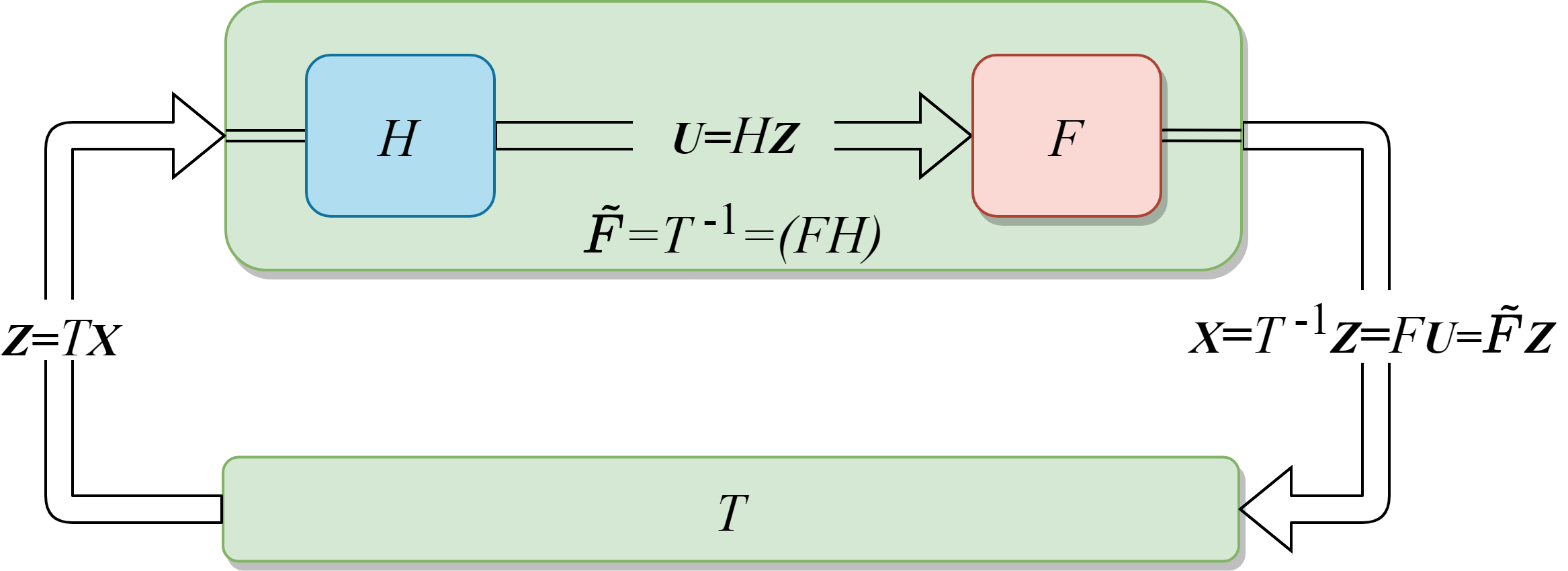
(c) c-GNF architecture for causal and counterfactual inference.

Figure 1: Fig. 1(a) shows temporal interactions between the treatments $A_{k}$ and the observed covariates/confounders $C_{k}$ at time-wave $k{=}1,\ldots,K$ and the outcome of interest $Y$. The solid edges indicate the cause and effect at the same time-wave and the dashed edges indicate the one time-wave delayed effect with respect to the respective causes. Fig. 1(b) represents the 2-wave model of Fig. 1(a). For any given observed endogenous variable $X$ in Fig. 1(b), $U_{X}$ and $Z_{X}$ respectively denote the unobserved exogenous noises of the true SCM $F{:}\mathbf{U}{\rightarrow}\mathbf{X}$ and the encapsulated-SCM $\tilde{F}{=}(FH){=}T^{-1}{:}\mathbf{Z}{\rightarrow}\mathbf{X}$ in Fig. 1(c), where $H{:}\mathbf{Z}{\rightarrow}\mathbf{U}$ denotes an auxiliary transformation. Since $\tilde{F}$ (green) encapsulates $F$ (red) and $H$ (blue) SCMs, i.e., $\tilde{F}{=}(FH){=}T^{-1}$, we refer to $\tilde{F}$ as the encapsulated-SCM. Our c-GNF models $T{:}\mathbf{X}{\rightarrow}\mathbf{Z}$ and readily provides the encapsulated-SCM $\tilde{F}{:}\mathbf{Z}{\rightarrow}\mathbf{X}$, as $T$ is invertible by construction, facilitating counterfactual inference using ‘The First Law of Causal Inference’ (pearl2009abductionactionprediction; pearl2009causality).

Since the realization that correlation does not imply causation (wright1921correlationcausation; fisher1936designofexperiments), statisticians, computer scientists, and social scientists have been developing ways to identify and estimate causal effects from observational data. By the 1970s, Structural Equation Models (SEMs), developed from Wright’s path analysis (wright1921correlationcausation) in genetics, have been widely used in economics (Haavelmo1943SEM; Goldberger1972SEMecon) and other social sciences (Duncan1974SEMsocio; Ploch1975SEM; Fienberg1975Introduction2SEM) to analyze cause and effect. Pearl’s Structural Causal Model (SCM) (pearl2009causality) provides an explicit causal definition to disambiguate the causes and effects by replacing the symmetric ‘=’ operator with asymmetric ‘:=’ assignment operator, thereby complementing the original SEM definition. Energized by this and similar developments in computer science, a causal revolution has occurred with large ramifications not only in academia but also for how governments, non-governmental organizations, and international organizations (such as the World Bank, United Nations Children’s Fund (UNICEF), or International Monetary Fund) articulate public policies to combat social ills. For example, to combat poverty, governments use mainly an individual’s income and similar characteristics to identify vulnerable population and then assess if they are eligible for social welfare eligibility. Then a simple rule is often applied: if they are eligible, they tend to receive a fixed one-size-fits-all public policy; if they are not eligible, no policy is ascribed. Although such public-policy making is highly transparent as it applies what is best on average for a population – that is the average causal effect (ACE) – it lacks an adaptability necessary to efficiently combat poverty, ill-health, and other social ills. For effective combating, government officials and others require methods that are able to personalize these policies (kino2021adelmlreview). That is, personalized public policy analysis (P³A) requires methods that can move beyond ACE estimation, and into counterfactual inference.

However, traditional statistical causal effect estimation methods, such as Inverse Probability Weighting (IPW) (Rosenbaum1983propensityscoreipw; hernan2009ipw) or recent ones such as Regression-With-Residuals (RWR) (wodtke2020rwr), focus on ACE estimation only. An advantage of IPW (stabilized) is that it provides a simple and effective way to estimate ACE without the need to model the entire causal system, under the assumption that the functional form of the propensity score is correctly specified. In contrast to IPW, RWR, which comes under the class of outcome regression models, estimate ACEs more effectively (less variance), under the assumption that the functional form of the outcome models are correctly specified. However due to the use of a single outcome model similar to S(Single)-Learner, RWR provides biased estimates when there is effect modification in data (also know as effect heterogeneity) (vanderweele2009distinctionheterogeneity).

To directly address effect modification, computer scientists have developed a class of outcome regression based machine-learning models called meta-learners (kunzel2019metalearners) (e.g., T(Two)-Learner, X-Learner) where each treatment group is modeled using a separate outcome regression models conditioned on proper adjustment sets to account for any confounding. Since meta-learners model separate conditional outcome regression models for each treatment groups, we alternatively refer them as Grouped Conditional Outcome Model (GCOM). The conditioning set or adjustment set or the predictors of outcome regression model are identified from the non-parametric expression of the interventional distribution obtained from $do$-calculus (pearl2009causality; pearl2012docalculus) or $G$-computation formula (ROBINS1986gcom; hernan2009ipw) to accurately model and estimate the causal effects of interest by adjusting for the confounding. While IPW requires the right propensity score model, RWR and GCOM methods require the correct outcome model. In contrast, Doubly Robust (DR) (bang2005doublyrobust) methods are a class of causal inference methods that incorporate the best of IPW and GCOM by jointly modeling the propensity score and the outcome. The key advantage of DR is that it requires only either one of the propensity or the outcome model to be correctly specified to produce unbiased ACE estimates. Notwithstanding the advantages of IPW, RWR, GCOM, and DR, none of them successfully supply a method to conduct counterfactual inference for P³A.

In this work, we aim to further P³A and causal inference in the social science by demonstrating a method for counterfactual inference that does not require a priori knowledge of the correct functional form in neither the propensity score or the outcome model. Our causal method consists of a flow-based deep learning approach known as Graphical Normalizing Flows (GNFs). As we re-purpose GNFs for causal inference by using causal-Directed Acyclic Graphs (causal-DAGs), we refer them as causal-GNFs (c-GNFs). Even though we focus on the social effect of neighborhood on children’s education outcomes (wodtke2020rwr) as an example of P³A in this article, our contributions are applicable to other settings in epidemiology, economics, sociology, and political science, where counterfactual policy-making is critical to promote social, material, and health outcomes. Our work supplies at least the following five contributions.

1. We show that c-GNF models the underlying SCM of interest in the form of an encapsulated-SCM using only the observational data and without making assumptions on the unobserved exogenous noises or the functional mechanisms of the true SCM. 2. Unlike IPW and RWR that require correct functional forms to provide unbiased ACEs, we show that c-GNF needs no functional form assumptions to achieve unbiasedness because the encapsulated-SCM, parameterized by a deep neural networks, has the ability to model any functional form from the observational data via likelihood maximization by gradient descent. 3. We demonstrate experimentally that c-GNF is on-par with IPW and RWR in terms of the bias and variance of the ACE estimates when the right functional forms are assumed and above-par when they are unknown under both small and large sample sizes. 4. Normalizing flows (NFs) are generally built for continuous variables. As this challenges the use of discrete variables, we propose a novel yet simple Gaussian dequantization trick to adapt discrete variables for NFs. 5. The most important, unique and key contribution of our c-GNF is that it has the capacity to perform counterfactual inference since c-GNF models the encapsulation of the true SCM. This enables scholars and policymakers to move beyond merely identifying the optimal treatment (public policy) at the population level and start tailoring individual-level optimal treatment (public policy). This capacity will advance P³A in social science and other domains (such as personalized medicine) (kino2021adelmlreview).

In the next section, we introduce the notations, define a typical social problem, and discuss the assumptions required to solve it. Then, we introduce c-GNFs, how they can be used to model SCMs, and how they estimate ACEs and counterfactual inference. Next, we present the simulated experimental setup, results and analysis. Lastly, we conclude our work with implications in social science and beyond.

Notation, Problem Definition and Assumptions

In this section, we discuss the formulation of the causal problem particularly in social science, notations, and critical assumptions for causal inference. Fig. 1(a) denotes the temporal model involving time-varying confounders used by wodtke2011ipw in their real-world study involving 16 waves or time-points, i.e., $k{=}1,\ldots,16$, where $A_{k}$ and $C_{k}$ denote the neighborhood context treatment and the observed neighborhood covariate at time $k$, and $Y$ denotes the high-school graduation as outcome of causal interest on the Panel Study of Income Dynamics (PSID) sensitive dataset (geolytics2003censuscdPSID). However, in this work, we consider the $2$-wave model in Fig. 1(b) used by wodtke2020rwr in his simulated experiments (non-sensitive data) such that the true causal effects are known for benchmarking of different causal effect estimation methods.

Specifically, our aim is same as that of wodtke2020rwr, i.e., to estimate the ACEs of the binary treatment variables $A_{1}$ and $A_{2}$ from the observational data. These ACEs ($\lambda_{a_{1},a_{2}}$) are formally defined as rCl λ_1,0 = E[Y_1,0]-E[Y_0,0]*
λ_0,1 = E[Y_0,1]-E[Y_0,0]
λ_1,1 = E[Y_1,1]-E[Y_1,0] where $Y_{a_{1},a_{2}}$ denotes the potential outcome of $Y$ under the interventions ${A_{1}}{:=}a_{1}$ and ${A_{2}}{:=}a_{2}$. Note that the previous expectations are with respect to the interventional distribution of $Y_{a_{1},a_{2}}$ under the interventions ${A_{1}}{:=}a_{1}$ and ${A_{2}}{:=}a_{2}$ rll P(Y_{a_k}^2_k=1) . Under the assumptions we discuss next, the interventional distribution in Eq. (Notation, Problem Definition and Assumptions) can be expressed in terms of the components from the observational joint distribution via $do$-calculus (pearl2012docalculus) or $G$-computation formula (ROBINS1986gcom; hernan2009ipw; pearl2009causality) as rll P(Y_{a_k}^2_k=1) &=∑_{C_k}^2_k=1P(Y—{C_k,a_k}^2_k=1) *
P(C_2—C_1,a_1) *
(Π_j=1^2 1_(A_j = a_j)) P(C_1) , where $1_{({A_{j}}{=}a_{j})}$ is the indicator function denoting the intervention ${A_{j}}{:=}a_{j}$. For the curious readers, the interventional distribution for the general $K$-wave model of wodtke2011ipw can be expressed analogously as rll P(Y_{a_k}^K_k=1)& =∑_{C_k}^K_k=1P(Y—{C_k,a_k}^K_k=1) *
(Π_j=2^K P(C_j—C_j-1,a_j-1)) *
(Π_j=1^K 1_(A_j = a_j)) P(C_1) .

Critical Assumptions in Causal Inference

Although generally ‘correlation does not imply causation’, causal inference is about defining under what assumptions and conditions correlation coincides with causation (pearl2009causality; neal2020Intro2CI). For our counterfactual-inference argument, we require six assumptions and conditions that are briefly stated below. The technical appendix shows detailing of the mathematical definitions and how causal quantities can be estimated from purely statistical quantities.

1. Unconfoundednessorno unobserved confounders: As shown in Fig. 1(a), we assume that there is no unobserved confounding between $A_{k}$ and $Y$. Otherwise, it is impossible to know if the observed correlation is due to causality or confounding. This assumption is strong and untestable (Rubin1990unconfoundedness). 2. Positivityoroverlaporcommon supportorextrapolation: We assume that every individual has non-zero probability of receiving any of the treatments, i.e., $P(A_{k}|A_{k-1},C_{k})$ is always positive. Otherwise, it is impossible to accurately estimate the causal effect as the model is inaccurate in the non-overlap region due to no data. 3. Conditional ignorability or exchangability: In economics and epidemiology, the assumptions of unconfoundedness and positivity are referred together as conditional ignorability or exchangability (Rosenbaum1983propensityscoreipw). Unconditional ignorability or exchangability can only be achieved in Randomized Controlled Trials (RCTs). 4. Consistency: This assumption states that the observed outcome is same as the potential outcome under the observed treatment (ROBINS1986gcom; cole2009consistency; vanderweele2009concerningconsistency). 5. No interferenceorStable Unit-Treatment Value Assumption (SUTVA): No interference means that a particular individual’s outcome is only a function of that particular individual’s treatment and is not affected by the treatment of any other individual (cox1958planning). 6. Modularityorindependent mechanismsorautonomyorinvariance: Any joint distribution can be factorized as the product of conditional distributions corresponding to independent causal mechanisms using the Markov assumption. Under the interventions, the modularity assumption states that all the mechanisms of the non-intervened variables remains the same while the mechanism of the intervened variables is set to the intervened value. The modularity assumption can be seen in Eqs. (Notation, Problem Definition and Assumptions) and (Notation, Problem Definition and Assumptions), where the probability terms corresponding to the mechanism of the intervened variable ${A_{j}}{:=}a_{j}$, i.e., $P(A_{j}|C_{j},A_{j-1})$ term in the observational joint distribution is replaced by the indicator function $1_{({A_{j}}{=}a_{j})}$ denoting the intervention ${A_{j}}{:=}a_{j}$. This modularity assumption is crucial for causal and counterfactual inference (pearl2009abductionactionprediction; pearl2009causality; pearl2018bookofwhy).

SCM, Encapsulated-SCM and c-GNF

In this section, we present our c-GNFs and describe their connection to SCMs. An SCM consists of a set of assignment equations describing the causal relations between the random variables of a causal system, such as rll X_i := f_i(PA_i, U_i) with i = 1,…,d where $\{X_{i}\}_{i{=}1}^{d}$ represents the set of observed endogenous random variables, $PA_{i}$ represents the set of variables that are connoting parents of $X_{i}$, $\{U_{i}\}_{i{=}1}^{d}$ denotes the set of exogenous noise random variables, and $\{f_{i}\}_{i{=}1}^{d}$ denotes the set of functions (independent mechanisms) that generate the endogenous variable $X_{i}$ from its observed causes $PA_{i}$ and noise $U_{i}$. SCM is also referred as Functional Causal Model (FCM) due to the functional mechanisms $\{f_{i}\}_{i{=}1}^{d}$.

Let $\mathbf{X}{=}[X_{1},\ldots,X_{d}]^{\text{T}}{\in}\mathbb{R}^{d}$ denote the $d$-dimensional vector of SCM endogenous variables. Similarly, let $\mathbf{U}{=}[U_{1},\ldots,U_{d}]^{\text{T}}{\in}\mathbb{R}^{d}$ denote the $d$-dimensional vector of SCM exogenous variables and $F{:}\mathbf{U}{\rightarrow}\mathbf{X}$ denote the transformation representing the true SCM such that $\mathbf{X}{=}F\mathbf{U}$. Let $\mathcal{G}$ represent a causal-DAG with $\{X_{1},\ldots,X_{d}\}$ as the set of nodes and adjacency matrix $\mathcal{A_{G}}{\in}\{0,1\}^{d{\times}d}$. Let $P_{\mathbf{X}}(\mathbf{X})$ represent the joint distribution over the endogenous variables $\mathbf{X}$, which factorizes according to the causal-DAG $\mathcal{G}$ as rll P_X(X) = Π_i=1^dP(X_i—PA_i) , where $PA_{i}{=}\{X_{j}{:}\mathcal{A_{G}}_{i,j}{=}1\}$ denotes the set of parents of the vertex/node $X_{i}$ in the causal-DAG $\mathcal{G}$. As we show in the next section, the factorized joint distribution in Eq. (SCM, Encapsulated-SCM and c-GNF) can be modeled using an autoregressive model parameterized by a deep-neural-network $\theta$, which we denote by $P_{\mathbf{X}}(\mathbf{X};\theta)$. Such a model is what we call c-GNF.

Causal-Graphical Normalizing Flows (c-GNFs)

Normalizing Flows (NFs) (tabak2010nf; tabak2013nf; rezende2015variationalNF; kobyzev2020NF; papamakarios2021NF_pmi) are a family of generative models with tractable distributions where both sampling and density evaluation can be efficient and exact. A NF is a flow-based model with transformation $T{:}\mathbf{X}{\rightarrow}\mathbf{Z}$, such that $\mathbf{Z}{=}T\mathbf{X}$, where $\mathbf{Z}{=}[Z_{1},\ldots,Z_{d}]^{\text{T}}{\in}\mathbb{R}^{d}$ represents the base random variable of the flow-model with the base distribution $P_{\mathbf{Z}}(\mathbf{Z})$ that is usually a $d$-dimensional standard normal distribution for computational convenience and ease of density estimation. Hence the name normalizing flow. The defining properties of $T$ are, (i) $T$ must be invertible with $T^{-1}$ as the inverse generative flow such that $T^{-1}{:}\mathbf{Z}{\rightarrow}\mathbf{X}$, and (ii) $T$ and $T^{-1}$ must be differentiable, i.e., $T$ must be a $d$-dimensional diffeomorphism (milnor1997diffeomorphism). Under these properties, from the change of variables formula, we can express the endogenous joint distribution $P_{\mathbf{X}}(\mathbf{X})$ in terms of the assumed base distribution $P_{\mathbf{Z}}(\mathbf{Z})$ as rll P_X(X) = P_Z(TX) —det J_T(X)— . Since calculating the joint density of $P_{\mathbf{X}}(\mathbf{X})$ requires the calculation of the determinant of the Jacobian of $T$ with respect to $\mathbf{X}$, i.e., $\mathrm{det}J_{T}(\mathbf{X})$, it is advantageous for computational reasons to choose $T$ to have an autoregressive structure such that $J_{T}(\mathbf{X})$ is a lower-triangular matrix and $\mathrm{det}J_{T}(\mathbf{X})$ is just the product of the diagonal elements. Autoregressive Flows (AFs) (kingma2016IAF; Papamakarios2017MAF; Huang2018NAF) are NFs that model autoregressive structure. AFs are composed of two components, the transformer and the conditioner (papamakarios2021NF_pmi). Under the assumption of a strictly monotonic transformer, AFs are universal density estimators (Huang2018NAF). Of all the current AFs, Graphical Normalizing Flows (GNFs) (wehenkel2020GNF) facilitate the use a desired DAG representation as opposed to an arbitrary autoregressive structure. For causal inference, it is crucial that the DAG has a causal interpretation. In this work, we assume the true causal-DAG $\mathcal{G}$ for the GNFs, hence the term causal-GNFs (c-GNFs). In c-GNFs, we use Unconstrained Monotonic Neural Network (UMNN) (wehenkel2019UMNN), a strictly monotonic integration based transformer with $\mathcal{G}$ for the graphical conditioner.

Since Markov equivalent DAGs induce equivalent factorizations of the observational joint distributions, GNFs that use Markov equivalent DAGs represent the same observational joint distribution. This is problematic for causal and counterfactual inference, as different GNFs may represent different interventional joint distributions. In other words, to perform causal inference as we do in this work, the GNF needs to use causal-DAG $\mathcal{G}$. Hence the name causal-GNF (c-GNF). To appreciate this, consider the Causal Autoregressive Flow (CAREFL) by khemakhem2021causalAF. While CAREFL uses AF, it is flawed as it considers all the predecessors in the topological ordering, i.e., a Markov equivalent DAG, when it should strictly be just the connoting parents/causes of the given node, i.e., the causal-DAG $\mathcal{G}$. We present an example of CAREFL’s flaw in our technical appendix, which shows the conditions under which CAREFL fails in counterfactual inference. Note that only a GNF with the true causal-DAG $\mathcal{G}$ encapsulates the true SCM, thus satisfying the modularity assumption, which is necessary for correct causal and counterfactual inference. This is formalized as rll X = FU = F(H(Z)) = (FH)Z = ~FZ = T^-1Z , where $H{:}\mathbf{Z}{\rightarrow}\mathbf{U}$ is an auxiliary transformation such that $U_{i}{=}h_{i}({Z_{i}})$ for $i{=}1,\ldots,d$ and $H{=}[h_{1},\ldots,h_{d}]^{\text{T}}$. It follows from Eq. (Causal-Graphical Normalizing Flows (c-GNFs)) that our c-GNF $T^{-1}{=}\tilde{F}{=}(FH)$ encapsulates the true SCM $F$ as $T$ and $T^{-1}$ both encode causal-DAG $\mathcal{G}$ in the graphical conditioner, thus providing a way to indirectly model $F$ without making assumptions on $\mathbf{U}$ or the functional causal mechanisms $F$ or the auxiliary transformation $H$. This sets apart our c-GNFs from most other models for causal inference. Fig. 1(c) shows the c-GNF architecture for causal and counterfactual inference using $T$ and $T^{-1}$.

Training a c-GNF amounts to training the deep neural networks that parameterize the transformers and conditioners. This is typically done by maximizing the $\log$-likelihood of the training dataset $\{\mathbf{X}^{\ell}\}^{N_{s}}_{\ell{=}1}$, which is expressed as shown below, by using Eq. (Causal-Graphical Normalizing Flows (c-GNFs)) for the summation term $P_{\mathbf{X}}(\mathbf{X}^{\ell};\theta)$ rll L(θ) = &∑_ℓ = 1^N_slogP_X(X^ℓ;θ) where $\theta$ denotes the parameters of the deep neural networks of the UMNN transformer and graphical conditioner, optimized using stochastic gradient descent.

Gaussian Dequantization Trick

Algorithm 1 Gaussian Dequantization and Quantization

1:procedure Gaussian Dequantization($\{{D^{\ell}}\}^{b}_{\ell{=}1}$)

2:     Generate $\tilde{D^{\ell}}\sim\mathcal{N}(\mu={D}^{\ell},\sigma^{2}=1/36)$

3:     return Dequantized / continuous variables $\{\tilde{D^{\ell}}\}^{b}_{\ell{=}1}$

4:end procedure

5:procedure Quantization($\{{\tilde{D}^{\ell}}\}^{b}_{\ell{=}1}$)

6:     ${D}^{\ell}=\mathrm{clamp}(\mathrm{round}(\tilde{D^{\ell}}),\mathrm{min}{=}0,\mathrm{max}{=}N{-}1)$

7:     return Quantized / discrete variables $\{{D^{\ell}}\}^{b}_{\ell{=}1}$

8:end procedure

NFs naturally model continuous variables, yet in practice, social scientists and others have to model both continuous and discrete variables, as treatments may be discrete categorical variables. Recently, discrete NFs have been an active field of research including techniques ranging from simple uniform dequantization, Gumbel-max dequantization to complex variational bound dequantization (Uria2013RNADETR_uniformdeq; Hoogeboom2019IDF; Tran2019IDF; ho2019flow++; ZieglerR2019VAE_dequant; Ma2019Macow; Nielsen2020DeqGap; Pawlowski2020DSCM_CI). Motivated by the Dirac-delta function from control theory, we propose and validate our novel Gaussian dequantization trick (see Algorithm 1 for a discrete variable $D$ with $N$ classes/categories) to model discrete variables into NFs using the fact that NFs are strongest in modeling Gaussian distributions seamlessly. We provide the exact motivation for the Gaussian dequantization and other details in the technical appendix.

Experiments, Results and Discussion

Figure 2: (a) $\{\theta_{11}{=}\theta_{21}{=}0,\gamma_{21}{=}\gamma_{12}{=}0\}$. (b) $\{\theta_{11}{=}\theta_{21}{=}0.2,\gamma_{21}{=}0.4,\gamma_{12}{=}0\}$. (c) $\{\theta_{11}{=}\theta_{21}{=}0.2,\gamma_{21}{=}\gamma_{12}{=}0.4\}$.

For our experiments and benchmarking, we simulate a virtual social system using the $2$-wave model shown in Fig. 1(b). We generated continuous covariates ($C_{1},C_{2}$), binary treatments ($A_{1},A_{2}$) and a continuous outcome $Y$. To provide a realistic sense to the virtual social system under our study, ($C_{1},C_{2}$) can denote the neighborhood contexts, e.g., the parental income of the individual in the given neighborhood, and ($A_{1},A_{2}$) can represents neighborhood exposures, e.g., rich/poor neighborhood, and $Y$ can represent the total score obtained in high-school graduation examination. Our aim is to analyse the neighborhood effects on the high-school graduation. We use the following governing equations from wodtke2020rwr to simulate the dataset. rCl C_1 & ∼ N(μ = 0, σ^2 = 1) , *
A_1 ∼ Bern(p = Φ(0.4C_1+2γ_12C^2_1)) ,
C_2 ∼ N(μ = 0.4C_1+0.2A_1, σ^2 = 1) ,
A_2 ∼ Bern(p = Φ(0.2A_1+0.4C_2+γ_12A^2_1
+2γ