Lorentz transformation in Maxwell equations for slowly moving media

Abstract

We use the method of field decomposition, a technique widely used in relativistic magnetohydrodynamics, to study the small velocity approximation (SVA) of the Lorentz transformation in Maxwell equations for slowly moving media. The “deformed” Maxwell equations derived under the SVA in the lab frame can be put into the conventional form of Maxwell equations in the medium’s comoving frame. Our results show that the Lorentz transformation in the SVA up to $O(v/c)$ ($v$ is the speed of the medium and $c$ is the speed of light in vacuum) is essential to derive these equations: the time and charge density must also change when transforming to a different frame even in the SVA, not just the position and current density as in the Galilean transformation. This marks the essential difference of the Lorentz transformation from the Galilean one. We show that the integral forms of Faraday and Ampere equations for slowly moving surfaces are consistent with Maxwell equations. We also present Faraday equation the covariant integral form in which the electromotive force can be defined as a Lorentz scalar independent of the observer’s frame. No evidences exist to support an extension or modification of Maxwell equations.

I Introduction

James Clerk Maxwell unified electricity and magnetism, the first unified theory of physics, by constructing a set of equations now known as Maxwell equations (maxwell:1861, ) (for the history of Maxwell equations, see, e.g., Ref. (Rautio:2014, )). Maxwell equations are the foundation of classical physics and many technologies that make the modern world. The Lorentz covariance is hidden in the structure of Maxwell equations, which was first disclosed by Albert Einstein in his well-known paper “On the electrodynamics of moving bodies” in 1905 that marked the discovery of special relativity (Einstein:1905ve, ; lorentz1904, ; poincare1906dynamique, ; poincare1906note, ).

Recently an extension of conventional Maxwell equations has been proposed to charged moving media (Wangzhonglin:2021, ) in order to describe the power output of piezoelectric and triboelectric nanogenerators (TENGs) (Wangzhonglin:20179, ; Wangzhonglin:201714, ; Wangzhonglin:2020104272, ), a new technology for fully utilizing the energy distributed in our living environment with low quality, low amplitude and even low frequency. The equations derived in Ref. (Wangzhonglin:2021, ) read (in cgs Gaussian unit and natural unit)

$$\boldsymbol{\nabla}\cdot\mathbf{B}(t,\mathbf{x}) = 0\,,$$

$$\boldsymbol{\nabla}\times\mathbf{E}(t,\mathbf{x}) = -\frac{1}{c}\left(\frac{\partial}{\partial t}+{\bf v}\cdot\boldsymbol{\nabla}\right)\mathbf{B}(t,\mathbf{x})\,,$$

$$\boldsymbol{\nabla}\cdot\mathbf{D}(t,\mathbf{x}) = \rho_{f}(t,\mathbf{x})\,,$$

$$\boldsymbol{\nabla}\times\mathbf{H}(t,\mathbf{x}) = \frac{1}{c}\mathbf{J}_{f}(t,\mathbf{x})+\frac{1}{c}\left(\frac{\partial}{\partial t}+{\bf v}\cdot\boldsymbol{\nabla}\right)\mathbf{D}(t,\mathbf{x})\,,$$ (1)

where $\mathbf{v}$ is the velocity of the medium and assumed to be much smaller than the speed of light $c$, and $\mathbf{D}=\mathbf{D}^{\prime}+\mathbf{P}_{s}$ with $\mathbf{D}^{\prime}$ being the conventional electric displacement field and $\mathbf{P}_{s}$ representing the polarization owing to the pre-existing electrostatic charges on the media induced by TENGs (Wangzhonglin:2021, ). The fields $\mathbf{E}$, $\mathbf{B}$, $\mathbf{D}^{\prime}$ and $\mathbf{H}$ are the electric, magnetic strength, electric displacement and magnetic fields in the observer’s frame (lab frame), respectively. Note that $\mathbf{P}_{s}$ is not linearly proportional to the electric field (Wangzhonglin:2021, ). The charge conservation law in Ref. (Wangzhonglin:2021, ) is modified to

$$\left(\frac{\partial}{\partial t}+{\bf v}\cdot\boldsymbol{\nabla}\right)\rho_{f}(t,\mathbf{x})+\boldsymbol{\nabla}\cdot\mathbf{J}_{f}(t,\mathbf{x})=0\,.$$ (2)

The differential equations in (1) were derived from an integral form of Maxwell equations (Wangzhonglin:2021, ). They are different from conventional Maxwell equations in two respects: (a) the appearance of the derivative operator $\partial/\partial t+{\bf v}\cdot\boldsymbol{\nabla}$ to replace $\partial/\partial t$; (b) the appearance of $\mathbf{P}_{s}$. The charge conservation law is different from the conventional one in (a).

It is obvious that the derivation of (1) and (2) is not based on the Lorentz transformation in special relativity. A natural question arises: can these equations in (1) except $\mathbf{P}_{s}$ be derived from the Lorentz transformation under the small velocity approximation (SVA)? The purpose of this paper is to answer this question.

In this paper, we use the (rationalized) cgs Gaussian unit (Landau:1984, ; Jackson:1998nia, ) in which electric and magnetic fields have the same unit: Gauss. In the rationalized cgs Gaussian unit, the irrational constant $4\pi$ is absent in Maxwell equations but appears in Coulomb and Ampere force laws among electric charges and currents respectively.

We work in the Minkowski space-time with the metric tensor $g^{\mu\nu}=g_{\mu\nu}=\mathrm{diag}(1,-1,-1,-1)$ where $\mu,\nu=0,1,2,3$, so that we can write space-time coordinates as $x=x^{\mu}=(x^{0},\mathbf{x})=(ct,\mathbf{x})$ and $x_{\mu}=(x_{0},-\mathbf{x})$ with $x_{0}=x^{0}=ct$. For a space position $\mathbf{x}=(\mathbf{x}_{1},\mathbf{x}_{2},\mathbf{x}_{3})$, we do not distinguish superscripts and subscripts of its components, $x^{i}=\mathbf{x}_{i}=\mathbf{x}^{i}$ for $i=1,2,3$. Normally we use Greek letters to denote four-dimensional indices of four-vectors and four-tensors, while their spatial components are denoted by space indices (Latin letters) $i,j,k,l,m,n=1,2,3$. The four-dimensional Levi-Civita symbols are denoted as $\epsilon^{\mu\nu\rho\sigma}$ and $\epsilon_{\mu\nu\rho\sigma}$ with the convention $\epsilon^{0123}=-\epsilon_{0123}=1$, while the three-dimensional Levi-Civita symbol is denoted as $\epsilon_{ijk}$ with the convention $\epsilon_{123}=1$.

II Field decomposition and Lorentz transformation

In the observer’s frame, the anti-symmetric strength tensor of the electromagnetic field is given by

$$F^{\mu\nu}=\partial^{\mu}A^{\nu}-\partial^{\nu}A^{\mu}\,,$$ (3)

where $x^{\mu}=(ct,\mathbf{x})$, $A^{\mu}=(A^{0},\mathbf{A})$, and $\partial^{\mu}=(c^{-1}\partial_{t},-\boldsymbol{\nabla})$ with $\partial^{0}\equiv c^{-1}\partial_{t}\equiv c^{-1}\partial/\partial t$ and $\partial^{i}=\partial/\partial x_{i}=-\partial/\partial\mathbf{x}_{i}\equiv-\boldsymbol{\nabla}_{i}$. The components of $F^{\mu\nu}$ are

$$F^{0i} = \partial^{0}A^{i}-\partial^{i}A^{0}=\frac{1}{c}\partial_{t}A^{i}+\nabla_{i}A^{0}=-\mathbf{E}_{i}\,,$$

$$F^{ij} = \partial^{i}A^{j}-\partial^{j}A^{i}=-\epsilon_{ijk}\mathbf{B}_{k}\,.$$ (4)

The components of $F_{\mu\nu}$ are then $F_{0i}=\mathbf{E}_{i}$ and $F_{ij}=-\epsilon_{ijk}\mathbf{B}_{k}$.

It is convenient to introduce a four-vector $u^{\mu}$ to decompose $F^{\mu\nu}(x)$ into the electric and magnetic field

$$F^{\mu\nu}(x)=\mathcal{E}^{\mu}(x)u^{\nu}-\mathcal{E}^{\nu}(x)u^{\mu}+\epsilon^{\mu\nu\rho\sigma}u_{\rho}\mathcal{B}_{\sigma}(x)\,,$$ (5)

where $\mathcal{E}^{\mu}$ and $\mathcal{B}^{\mu}$ are four-vectors constructed from the electric and magnetic field respectively. Note that $u^{\mu}$ corresponds to the four-velocity $cu^{\mu}$ and satisfies $u_{\mu}u^{\mu}=1$, we also assume that it is a space-time constant. They can be extracted from $F^{\mu\nu}$ by

$$\mathcal{E}^{\mu} = F^{\mu\nu}u_{\nu}\,,$$

$$\mathcal{B}^{\mu} = \frac{1}{2}\epsilon^{\mu\nu\rho\sigma}u_{\nu}F_{\rho\sigma}\equiv\widetilde{F}^{\mu\nu}u_{\nu}\,,$$ (6)

where $\widetilde{F}^{\mu\nu}=(1/2)\epsilon^{\mu\nu\alpha\beta}F_{\alpha\beta}$ is the dual of the field strength tensor. The field decomposition (5) is widely used in relativistic magnetohydrodynamics (Giacomazzo:2005jy, ; Huang:2011dc, ; Pu:2016ayh, ; Denicol:2018rbw, ). The Lorentz transformation of $F^{\mu\nu}$ can be realized by that of four-vectors $\mathcal{E}^{\mu}$, $\mathcal{B}^{\mu}$ and $u^{\mu}$,

$$F^{\prime\mu\nu}(x^{\prime}) = \Lambda_{\;\alpha}^{\mu}\Lambda_{\;\beta}^{\nu}F^{\alpha\beta}(x)$$ (7)

$$= \Lambda_{\;\alpha}^{\mu}\Lambda_{\;\beta}^{\nu}\left[\mathcal{E}^{\alpha}(x)u^{\beta}-\mathcal{E}^{\beta}(x)u^{\alpha}+\epsilon^{\alpha\beta\rho\sigma}u_{\rho}\mathcal{B}_{\sigma}(x)\right]$$

$$= \mathcal{E}^{\prime\mu}(x^{\prime})u^{\prime\nu}-\mathcal{E}^{\prime\nu}(x^{\prime})u^{\prime\mu}+\epsilon^{\mu\nu\rho\sigma}u_{\rho}^{\prime}\mathcal{B}_{\sigma}^{\prime}(x^{\prime})\,,$$

where $\Lambda_{\;\alpha}^{\mu}$ denotes the Lorentz transformation tensor and $\mathcal{E}^{\mu}(x)$ and $\mathcal{B}^{\mu}(x)$ are transformed as four-vectors $\mathcal{E}^{\prime\mu}(x^{\prime})=\Lambda_{\;\alpha}^{\mu}\mathcal{E}^{\alpha}(x)$ and $\mathcal{B}^{\prime\mu}(x^{\prime})=\Lambda_{\;\alpha}^{\mu}\mathcal{B}^{\alpha}(x)$. It seems that the degrees of freedom of $F^{\mu\nu}$ would be increased because $\mathcal{E}^{\mu}$ and $\mathcal{B}^{\mu}$ are four-vectors and would have 8 independent variables. However this is not true since $\mathcal{E}^{\mu}$ and $\mathcal{B}^{\mu}$ are orthogonal to $u^{\mu}$, i.e. $\mathcal{E}\cdot u=\mathcal{B}\cdot u=0$.

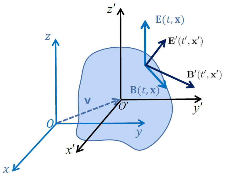
Figure 1: The lab or observer’s frame and the comoving frame of the medium. The comoving frame moves at a three-velocity $\mathbf{v}$ relative to the lab frame. All fields and space-time in the comoving frame are labeled with primes.

We have a freedom to choose any $u^{\mu}$ to make the decomposition (5) for $F^{\mu\nu}(x)$. As the simplest choice, we take $u^{\mu}=u_{L}^{\mu}\equiv(1,\mathbf{0})$, which corresponds to the lab or observer’s frame as shown in Fig. 1. Then Eq. (5) has the form

$$F^{\mu\nu}(x)=\mathcal{E}_{L}^{\mu}(x)u_{L}^{\nu}-\mathcal{E}_{L}^{\nu}(x)u_{L}^{\mu}+\epsilon^{\mu\nu\rho\sigma}u_{L\rho}\mathcal{B}_{L\sigma}(x)\,,$$ (8)

where $\mathcal{E}_{L}^{\mu}=(0,E^{1},E^{2},E^{3})=(0,\mathbf{E})$ and $\mathcal{B}_{L}^{\mu}=(0,B^{1},B^{2},B^{3})=(0,\mathbf{B})$. The matrix form of $F^{\mu\nu}$ corresponding to $u_{L}^{\mu}$ is then

$$F^{\mu\nu}=\left(\begin{array}[]{cccc}0&-E^{1}&-E^{2}&-E^{3}\\ E^{1}&0&-B^{3}&B^{2}\\ E^{2}&B^{3}&0&-B^{1}\\ E^{3}&-B^{2}&B^{1}&0\end{array}\right)\,,$$ (9)

which is just the matrix form of Eq. (4).

As a second choice, we take $u^{\mu}=\gamma(1,\mathbf{v}/c)$ with $\gamma=(1-v^{2}/c^{2})^{-1/2}$ being the Lorentz factor and $v\equiv|\mathbf{v}|$ being a three-velocity. In this case the electric and magnetic field four-vectors are given by

$$\mathcal{E}^{\mu}(x) = \gamma F^{\mu 0}(x)-\gamma\frac{v_{j}}{c}F^{\mu j}(x)$$

$$= \gamma\left(\frac{\mathbf{v}}{c}\cdot\mathbf{E},\mathbf{E}+\frac{\mathbf{v}}{c}\times\mathbf{B}\right)=\left(\frac{\mathbf{v}}{c}\cdot\boldsymbol{\mathcal{E}},\boldsymbol{\mathcal{E}}\right)\,,$$

$$\mathcal{B}^{\mu}(x) = \frac{1}{2}\gamma\epsilon^{\mu 0\rho\sigma}F_{\rho\sigma}(x)-\frac{1}{2}\gamma\frac{v_{i}}{c}\epsilon^{\mu i\rho\sigma}F_{\rho\sigma}(x)$$ (10)

$$= \gamma\left(\frac{\mathbf{v}}{c}\cdot\mathbf{B},\mathbf{B}-\frac{\mathbf{v}}{c}\times\mathbf{E}\right)=\left(\frac{\mathbf{v}}{c}\cdot\boldsymbol{\mathcal{B}},\boldsymbol{\mathcal{B}}\right)\,,$$

where $\mathbf{E}$, $\mathbf{B}$, $\boldsymbol{\mathcal{E}}$ and $\boldsymbol{\mathcal{B}}$ are all functions of $x=(ct,\mathbf{x})$. We note that $\mathcal{E}^{\mu}(x)$ and $\mathcal{B}^{\mu}(x)$ are space-time four-vectors. We now make the Lorentz transformation for $\mathcal{E}^{\mu}(x)$ and $\mathcal{B}^{\mu}(x)$ to the comoving frame of the medium which moves with $\mathbf{v}$ relative to the Lab frame (see in Fig. 1), so we have

$$\mathcal{E}^{\prime\mu}(x^{\prime}) = \Lambda_{\;\alpha}^{\mu}(\mathbf{v})\mathcal{E}^{\alpha}(x)\,,$$

$$\mathcal{B}^{\prime\mu}(x^{\prime}) = \Lambda_{\;\alpha}^{\mu}(\mathbf{v})\mathcal{B}^{\alpha}(x)\,,$$ (11)

where $x^{\prime\mu}=\Lambda_{\;\alpha}^{\mu}(\mathbf{v})x^{\alpha}$. With $u^{\prime\mu}=\Lambda_{\;\alpha}^{\mu}(\mathbf{v})u^{\alpha}=u_{L}^{\mu}$, the transformation of $F^{\mu\nu}$ following Eq. (7) reads

$$F^{\prime\mu\nu}(x^{\prime})=\mathcal{E}^{\prime\mu}(x^{\prime})u_{L}^{\nu}-\mathcal{E}^{\prime\nu}(x^{\prime})u_{L}^{\mu}+\epsilon^{\mu\nu\rho\sigma}u_{L\rho}\mathcal{B}_{\sigma}^{\prime}(x^{\prime})\,.$$ (12)

On the other hand, using $u_{L}^{\mu}$, $F^{\prime\mu\nu}(x^{\prime})$ can be rewritten as

$$F^{\prime\mu\nu}(x^{\prime})=\mathcal{E}_{L}^{\prime\mu}(x^{\prime})u_{L}^{\nu}-\mathcal{E}_{L}^{\prime\nu}(x^{\prime})u_{L}^{\mu}+\epsilon^{\mu\nu\rho\sigma}u_{L\rho}\mathcal{B}_{L\sigma}^{\prime}(x^{\prime})\,.$$ (13)

Comparing Eq. (12) with (13) we obtain

$$\mathcal{E}^{\prime\mu}(x^{\prime}) = \mathcal{E}_{L}^{\prime\mu}(x^{\prime})=(0,\mathbf{E}^{\prime}(x^{\prime}))\,,$$

$$\mathcal{B}^{\prime\mu}(x^{\prime}) = \mathcal{B}_{L}^{\prime\mu}(x^{\prime})=(0,\mathbf{B}^{\prime}(x^{\prime}))\,,$$ (14)

where $\mathbf{E}^{\prime}(x^{\prime})$ and $\mathbf{B}^{\prime}(x^{\prime})$ are the Lorentz-transformed electric and magnetic field in the moving frame

$$\mathbf{E}^{\prime}(x^{\prime}) = \gamma\left[\mathbf{E}(x)+\frac{\mathbf{v}}{c}\times\mathbf{B}(x)\right]+(1-\gamma)\mathbf{E}_{\parallel}(x)$$

$$= \gamma\left[\mathbf{E}_{\perp}(x)+\frac{\mathbf{v}}{c}\times\mathbf{B}(x)\right]+\mathbf{E}_{\parallel}(x)\,,$$

$$\mathbf{B}^{\prime}(x^{\prime}) = \gamma\left[\mathbf{B}(x)-\frac{\mathbf{v}}{c}\times\mathbf{E}(x)\right]+(1-\gamma)\mathbf{B}_{\parallel}(x)$$ (15)

$$= \gamma\left[\mathbf{B}_{\perp}(x)-\frac{\mathbf{v}}{c}\times\mathbf{E}(x)\right]+\mathbf{B}_{\parallel}(x)\,,$$

where $\mathbf{Y}_{\parallel}=\widehat{\mathbf{v}}(\widehat{\mathbf{v}}\cdot\mathbf{Y})$ and $\mathbf{Y}_{\perp}=(1-\widehat{\mathbf{v}}\widehat{\mathbf{v}})\cdot\mathbf{Y}$ are the parallel and perpendicular part of a three-vector $\mathbf{Y}=\mathbf{E},\mathbf{B}$ to the direction $\widehat{\mathbf{v}}$ of $\mathbf{v}$. Comparing the exact Lorentz transformation (15) with $\boldsymbol{\mathcal{E}}$ and $\boldsymbol{\mathcal{B}}$ in Eq. (10), we see the terms proportional to $1-\gamma=-[\gamma^{2}/(1+\gamma)](v^{2}/c^{2})\sim v^{2}/c^{2}$ are neglected in Eq. (10) because we only consider the SVA up to $O(v/c)$.

III Maxwell equations

The covariant form of Maxwell equations in vacuum reads

$$\partial_{\mu}\widetilde{F}^{\mu\nu}(x) = 0\,,$$ (16)

$$\partial_{\mu}F^{\mu\nu}(x) = \frac{1}{c}J^{\nu}(x)\,,$$ (17)

where $J^{\nu}=(cJ^{0},\mathbf{J})=(c\rho,\mathbf{J})$ is the four-current density. The homogeneous equation (16) gives Faraday’s law and divergence-free property of the magnetic field, while Eq. (17) gives Coulomb’s and Ampere’s laws. So from Eqs. (16) and (17), we obtain the conventional form of Maxwell equations in vacuum

$$\boldsymbol{\nabla}\cdot\mathbf{B}(x) = 0\,,$$

$$\boldsymbol{\nabla}\times\mathbf{E}(x) = -\frac{1}{c}\frac{\partial\mathbf{B}(x)}{\partial t}\,,$$

$$\boldsymbol{\nabla}\cdot\mathbf{E}(x) = \rho(x)\,,$$

$$\boldsymbol{\nabla}\times\mathbf{B}(x) = \frac{1}{c}\mathbf{J}(x)+\frac{1}{c}\frac{\partial\mathbf{E}(x)}{\partial t}\,,$$ (18)

where all fields are functions of $x=(ct,\mathbf{x})$. The derivation of Eq. (18) from Eqs. (16) and (17) is given in Appendix A.

In the presence of medium, one can introduce the tensor $M^{\mu\nu}$ describing the polarization and magnetization of the medium. Similar to $F^{\mu\nu}$ in Eq. (5), the decomposition of $M^{\mu\nu}$ is in the following form

$$M^{\mu\nu}=-(\mathcal{P}^{\mu}u^{\nu}-\mathcal{P}^{\nu}u^{\mu})+\epsilon^{\mu\nu\rho\sigma}u_{\rho}\mathcal{M}_{\sigma}(x)\,,$$ (19)

where $\mathcal{P}^{\mu}$ and $\mathcal{M}^{\mu}$ are the polarization and magnetization four-vector respectively. Note that there is a sign difference between $\mathcal{P}^{\mu}$ in the above formula and $\mathcal{E}^{\mu}$ in Eq. (5). Similar to Eq. (6), $\mathcal{P}^{\mu}$ and $\mathcal{M}^{\mu}$ can be extracted from $M^{\mu\nu}$ as

$$\mathcal{P}^{\mu} = -M^{\mu\nu}u_{\nu}\,,$$

$$\mathcal{M}^{\mu} = \frac{1}{2}\epsilon^{\mu\nu\rho\sigma}u_{\nu}M_{\rho\sigma}\,.$$ (20)

Then we can define the Faraday field tensor $H^{\mu\nu}$ as

$$H^{\mu\nu} = F^{\mu\nu}-M^{\mu\nu}$$ (21)

$$= \mathcal{D}^{\mu}(x)u^{\nu}-\mathcal{D}^{\nu}(x)u^{\mu}+\epsilon^{\mu\nu\rho\sigma}u_{\rho}\mathcal{H}_{\sigma}(x)\,,$$

where $\mathcal{D}^{\mu}$ and $\mathcal{H}^{\mu}$ are the electric displacement and magnetic field four-vector in the medium respectively and defined by

$$\mathcal{D}^{\mu} = \mathcal{E}^{\mu}+\mathcal{P}^{\mu}\,,$$

$$\mathcal{H}^{\mu} = \mathcal{B}^{\mu}-\mathcal{M}^{\mu}\,.$$ (22)

For homogeneous and isotropic dielectric and magnetic materials, we have following constitutive relations (minkowski1908, ; minkowski1910, ; einstein1908elektromagnetischen, ; pauli1981theory, )

$$\mathcal{D}^{\mu} = \epsilon\mathcal{E}^{\mu}\,,$$

$$\mathcal{H}^{\mu} = \frac{1}{\mu}\mathcal{B}^{\mu}\,,$$ (23)

where $\epsilon$ is the electric permittivity (it is $\epsilon_{0}=1$ in vacuum) and $\mu$ is the magnetic permeability (it is $\mu_{0}=1$ in vacuum) of the medium. Note that we use cgs Gaussian unit, $\epsilon$ and $\mu$ correspond to the relative permittivity and permeability in SI unit respectively. In terms of $F^{\mu\nu}$ and $H^{\mu\nu}$, we have Maxwell equations in the polarized and magnetized medium

$$\partial_{\mu}\widetilde{F}^{\mu\nu}(x) = 0\,,$$ (24)

$$\partial_{\mu}H^{\mu\nu}(x) = \frac{1}{c}J_{f}^{\nu}(x)\,,$$ (25)

where $J_{f}^{\mu}=(c\rho_{f},\mathbf{J}_{f})$ denotes the free four-current density with $\rho_{f}$ and $\mathbf{J}_{f}$ being the free charge and three-current densities. The only difference from Maxwell equations in vacuum is the appearance of $H^{\mu\nu}$ in the equation with the current instead of $F^{\mu\nu}$. In the presence of dielectric and magnetic media, we can also obtain the similar equations or relations for $\mathcal{D}^{\mu}$ and $\mathcal{H}^{\mu}$ as components of $H^{\mu\nu}$ to Eqs. (10)-(15) in Sect. II.

Corresponding to covariant Maxwell equations (24) and (25) in dielectric and magnetic media, we have Maxwell equations in the three-dimensional form

$$\boldsymbol{\nabla}\cdot\mathbf{B}(x) = 0\,,$$

$$\boldsymbol{\nabla}\times\mathbf{E}(x) = -\frac{1}{c}\frac{\partial\mathbf{B}(x)}{\partial t}\,,$$

$$\boldsymbol{\nabla}\cdot\mathbf{D}(x) = \rho_{f}(x)\,,$$

$$\boldsymbol{\nabla}\times\mathbf{H}(x) = \frac{1}{c}\mathbf{J}_{f}(x)+\frac{1}{c}\frac{\partial\mathbf{D}(x)}{\partial t}\,.$$ (26)

The derivation of (26) from Eqs. (24) and (25) is similar to that of Eq. (18) in Appendix A.

IV SVA of Maxwell equations in moving frame

We take the SVA in Eqs. (10) and (15) by neglecting all $O(v^{2})$ terms which is equivalent to setting $\gamma\approx 1$, and we obtain

$$\boldsymbol{\mathcal{E}}(x) \approx {\bf E}^{\prime}(x^{\prime})\approx{\bf E}(x)+\frac{{\bf v}}{c}\times{\bf B}(x)\,,$$

$$\boldsymbol{\mathcal{B}}(x) \approx {\bf B}^{\prime}(x^{\prime})\approx{\bf B}(x)-\frac{{\bf v}}{c}\times{\bf E}(x)\,,$$ (27)

where $\boldsymbol{\mathcal{E}}$ and $\boldsymbol{\mathcal{B}}$ are the spatial components of $\mathcal{E}^{\mu}$ and $\mathcal{B}^{\mu}$ in (10) respectively. This indicates that $\boldsymbol{\mathcal{E}}(x)$ and $\boldsymbol{\mathcal{B}}(x)$ are the same as those used in Eq. (2.9) in Ref. (wang2022relativistic, ). Similarly we also have

$$\boldsymbol{\mathcal{D}}(x) \approx\mathbf{D}^{\prime}(x^{\prime})\approx{\bf D}(x)+\frac{{\bf v}}{c}\times{\bf H}(x),$$

$$\boldsymbol{\mathcal{H}}(x) \approx\mathbf{H}^{\prime}(x^{\prime})\approx{\bf H}(x)-\frac{{\bf v}}{c}\times{\bf D}(x).$$ (28)

in the presence of dielectric and magnetic media.

In order to derive Maxwell equations in terms of $\boldsymbol{\mathcal{E}}(x)$ and $\boldsymbol{\mathcal{B}}(x)$ in the SVA we can insert $F^{\mu\nu}$ in (5) with $u^{\mu}=\gamma(1,\mathbf{v}/c)$ into Eqs. (16) and (17), the covariant Maxwell equations in vacuum. The resulting equations in three-dimensional form read

$$\left(\boldsymbol{\nabla}+\frac{{\bf v}}{c^{2}}\frac{\partial}{\partial t}\right)\cdot\boldsymbol{\mathcal{B}}(x) = 0\,,$$

$$\left(\boldsymbol{\nabla}+\frac{{\bf v}}{c^{2}}\frac{\partial}{\partial t}\right)\times\boldsymbol{\mathcal{E}}(x) = -\frac{1}{c}\left(\frac{\partial}{\partial t}+{\bf v}\cdot\boldsymbol{\nabla}\right)\boldsymbol{\mathcal{B}}(x)\,,$$

$$\left(\boldsymbol{\nabla}+\frac{{\bf v}}{c^{2}}\frac{\partial}{\partial t}\right)\cdot\boldsymbol{\mathcal{E}}(x) = \rho(x)-\frac{1}{c^{2}}{\bf v}\cdot{\bf J}(x)\,,$$

$$\left(\boldsymbol{\nabla}+\frac{{\bf v}}{c^{2}}\frac{\partial}{\partial t}\right)\times\boldsymbol{\mathcal{B}}(x) = \frac{1}{c}\left[{\bf J}(x)-\rho(x){\bf v}\right]+\frac{1}{c}\left(\frac{\partial}{\partial t}+{\bf v}\cdot\boldsymbol{\nabla}\right)\boldsymbol{\mathcal{E}}(x)\,.$$ (29)

The derivation of above equations from Eqs. (16) and (17) is given in Appendix B.

In the presence of homogeneous and isotropic dielectric and magnetic materials with the constitutive relations (23), we should start from Eq. (25) aided by the decomposition of $H^{\mu\nu}$ in (21) to obtain non-homogeneous Maxwell equations under the SVA. The homogeneous equation (24) remain the same as that in vacuum and gives the first two equations of (29) under the SVA. The resulting Maxwell equations for moving media now read

$$\left(\boldsymbol{\nabla}+\frac{{\bf v}}{c^{2}}\frac{\partial}{\partial t}\right)\cdot\boldsymbol{\mathcal{B}}(x) = 0\,,$$

$$\left(\boldsymbol{\nabla}+\frac{{\bf v}}{c^{2}}\frac{\partial}{\partial t}\right)\times\boldsymbol{\mathcal{E}}(x) = -\frac{1}{c}\left(\frac{\partial}{\partial t}+{\bf v}\cdot\boldsymbol{\nabla}\right)\boldsymbol{\mathcal{B}}(x)\,,$$

$$\left(\boldsymbol{\nabla}+\frac{{\bf v}}{c^{2}}\frac{\partial}{\partial t}\right)\cdot\boldsymbol{\mathcal{D}}(x) = \rho_{f}(x)-\frac{1}{c^{2}}{\bf v}\cdot{\bf J}_{f}(x)\,,$$

$$\left(\boldsymbol{\nabla}+\frac{{\bf v}}{c^{2}}\frac{\partial}{\partial t}\right)\times\boldsymbol{\mathcal{H}}(x) = \frac{1}{c}\left[{\bf J}_{f}(x)-\rho_{f}(x){\bf v}\right]+\frac{1}{c}\left(\frac{\partial}{\partial t}+{\bf v}\cdot\boldsymbol{\nabla}\right)\boldsymbol{\mathcal{D}}(x)\,.$$ (30)

The derivation of above equations is similar to that of Eq. (29) which is given in Appendix B. Equations in (30) are Maxwell equations in slowly moving media seen in the lab frame. We can check the charge conservation law by acting the operator $\boldsymbol{\nabla}+(1/c^{2}){\bf v}(\partial/\partial t)$ on the fourth equation and using the third equation of (30) as

$$\left(\boldsymbol{\nabla}+\frac{{\bf v}}{c^{2}}\frac{\partial}{\partial t}\right)\cdot\left[{\bf J}_{f}(x)-\rho_{f}(x){\bf v}\right]+\left(\frac{\partial}{\partial t}+{\bf v}\cdot\boldsymbol{\nabla}\right)\left[\rho_{f}(x)-\frac{1}{c^{2}}{\bf v}\cdot{\bf J}_{f}(x)\right]=0\,,$$ (31)

which is equivalent to the charge conservation law in the lab frame up to $O(v/c)$,

$$\frac{\partial}{\partial t}\rho_{f}(x)+\boldsymbol{\nabla}\cdot{\bf J}_{f}(x)=0\,.$$ (32)

Note that all terms of $O(v/c)$ cancel in Eq. (31). In deriving Eq. (31) we have used the commutability of two derivative operators

$$\left(\boldsymbol{\nabla}+\frac{{\bf v}}{c^{2}}\frac{\partial}{\partial t}\right)\left(\frac{\partial}{\partial t}+{\bf v}\cdot\boldsymbol{\nabla}\right) = \left(\frac{\partial}{\partial t}+{\bf v}\cdot\boldsymbol{\nabla}\right)\left(\boldsymbol{\nabla}+\frac{{\bf v}}{c^{2}}\frac{\partial}{\partial t}\right)\,,$$ (33)

for constant $\mathbf{v}$.

We can express ${\bf E}$ and ${\bf B}$ in terms of $\boldsymbol{\mathcal{E}}$ and $\boldsymbol{\mathcal{B}}$ using Eq. (10), and express ${\bf D}$ and ${\bf H}$ in terms of $\boldsymbol{\mathcal{D}}$ and $\boldsymbol{\mathcal{H}}$ in a similar way. In the SVA up to $O(v/c)$, we take $\gamma\approx 1$ and drop $O(v^{2}/c^{2})$ terms to obtain

$${\bf E}(x) \approx \boldsymbol{\mathcal{E}}(x)-\frac{{\bf v}}{c}\times\boldsymbol{\mathcal{B}}(x)\,,$$

$${\bf B}(x) \approx \boldsymbol{\mathcal{B}}(x)+\frac{{\bf v}}{c}\times\boldsymbol{\mathcal{E}}(x)\,,$$ (34)

$${\bf D}(x) \approx \boldsymbol{\mathcal{D}}(x)-\frac{{\bf v}}{c}\times\boldsymbol{\mathcal{H}}(x)\,,$$

$${\bf H}(x) \approx \boldsymbol{\mathcal{H}}(x)+\frac{{\bf v}}{c}\times\boldsymbol{\mathcal{D}}(x)\,.$$ (35)

By inserting Eqs. (34) and (35) into three-dimensional Maxwell equations (18) and (26) respectively and neglecting terms of $O(v^{2}/c^{2})$, one can also obtain Eqs. (29) and (30) similar to the method used in Refs. (wang2022relativistic, ; li2022comments, ).

Lorentz	Lorentz [SVA up to $O(v/c)$]	Galilean
$t^{\prime}=\gamma(t-\frac{{\bf v}}{c^{2}}\cdot{\bf x})$	$t^{\prime}\approx t-\frac{{\bf v}}{c^{2}}\cdot{\bf x}$	$t^{\prime}=t$$\;\;\;\;\;\;\;\;\;\;\;\;(*)$
$\boldsymbol{\nabla}^{\prime}=\gamma\left(\boldsymbol{\nabla}+\frac{{\bf v}}{c^{2}}\frac{\partial}{\partial t}\right)$	$\boldsymbol{\nabla}^{\prime}\approx\boldsymbol{\nabla}+\frac{{\bf v}}{c^{2}}\frac{\partial}{\partial t}$	$\boldsymbol{\nabla}^{\prime}=\boldsymbol{\nabla}$$\;\;\;\;\;\;\;\;\;\;\;\;(*)$
$\rho^{\prime}(x^{\prime})=\gamma\left[\rho(x)-\frac{{\bf v}}{c^{2}}\cdot{\bf J}(x)\right]$	$\rho^{\prime}(x^{\prime})\approx\rho(x)-\frac{{\bf v}}{c^{2}}\cdot{\bf J}(x)$	$\rho^{\prime}(x^{\prime})=\rho(x)$$\;\;\;\;\;\;\;\;\;\;\;\;(*)$
${\bf x}^{\prime}=\gamma({\bf x}-{\bf v}t)$	${\bf x}^{\prime}\approx{\bf x}-{\bf v}t$	${\bf x}^{\prime}={\bf x}-{\bf v}t$
$\frac{\partial}{\partial t^{\prime}}=\gamma\left(\frac{\partial}{\partial t}+{\bf v}\cdot\boldsymbol{\nabla}\right)$	$\frac{\partial}{\partial t^{\prime}}\approx\frac{\partial}{\partial t}+{\bf v}\cdot\boldsymbol{\nabla}$	$\frac{\partial}{\partial t^{\prime}}=\frac{\partial}{\partial t}+{\bf v}\cdot\boldsymbol{\nabla}$
${\bf J}^{\prime}(x^{\prime})=\gamma\left[{\bf J}(x)-{\bf v}\rho(x)\right]$	${\bf J}^{\prime}(x^{\prime})\approx{\bf J}(x)-{\bf v}\rho(x)$	${\bf J}^{\prime}(x^{\prime})={\bf J}(x)-{\bf v}\rho(x)$

Table 1: The Lorentz transformation, its SVA up to $O(v/c)$ and Galilean transformation for some quantities and derivative operators. The Galilean transformation differs from the SVA of the Lorentz transformation in the first three rows which are labeled by “$(*)$”. The Lorentz transformation reduces to the Galilean one for $x^{\mu}=(ct,\mathbf{x})$ in two conditions (doi:10.1121/1.1912121, ): (a) $v/c\rightarrow 0$; (b) $|\mathbf{x}|\sim vt$, so does for $J^{\mu}=(c\rho,\mathbf{J})$.

We can rewrite Eq. (30) in a compact form if we replace $\boldsymbol{\mathcal{E}}(x)$, $\boldsymbol{\mathcal{B}}(x)$, $\boldsymbol{\mathcal{D}}(x)$ and $\boldsymbol{\mathcal{H}}(x)$ by ${\bf E}^{\prime}(x^{\prime})$, ${\bf B}^{\prime}(x^{\prime})$, ${\bf D}^{\prime}(x^{\prime})$ and ${\bf H}^{\prime}(x^{\prime})$ following Eqs. (27) and (28). The resulting equations read

$$\boldsymbol{\nabla}^{\prime}\cdot{\bf B}^{\prime}(x^{\prime}) = 0\,,$$

$$\boldsymbol{\nabla}^{\prime}\times{\bf E}^{\prime}(x^{\prime}) = -\frac{1}{c}\frac{\partial}{\partial t^{\prime}}{\bf B}^{\prime}(x^{\prime})\,,$$

$$\boldsymbol{\nabla}^{\prime}\cdot{\bf D}^{\prime}(x^{\prime}) = \rho_{f}^{\prime}(x^{\prime})\,,$$

$$\boldsymbol{\nabla}^{\prime}\times{\bf H}^{\prime}(x^{\prime}) = \frac{1}{c}{\bf J}_{f}^{\prime}(x^{\prime})+\frac{1}{c}\frac{\partial}{\partial t^{\prime}}{\bf D}^{\prime}(x^{\prime})\,,$$ (36)

where we have used the Lorentz transformation in the SVA up to $O(v/c)$ for quantities and operators listed in the second column of Table 1. Also we can rewrite the charge conservation law (31) in terms of quantities in the comoving frame

$$\frac{\partial}{\partial t^{\prime}}\rho_{f}^{\prime}(x^{\prime})+\boldsymbol{\nabla}^{\prime}\cdot{\bf J}_{f}^{\prime}(x^{\prime})=0\,,$$ (37)

which can be proved by taking a divergence $\boldsymbol{\nabla}^{\prime}$ of the fourth equation and using the third equation of (36). We see in Table 1 that the Lorentz transformation in the SVA obviously differs from the Galilean transformation in the first three rows: the time, the charge density and the space-derivative operator $\boldsymbol{\nabla}$ are not invariant in the former, while they are invariant in the latter. However, different from the cases of the space-time and charge-current density, the Galilean transformation of electric and magnetic fields is not well-defined, see, e.g., Refs. (bellac:1973, ; daixi:2022, ; daixi:2022en, ) for discussions of this topic.

Equation (36) is nothing but Maxwell equations in the comoving frame of the medium. It is not surprising that Maxwell equations have the same form in the comoving frame as shown in (36). However, what makes Eq. (30) [another form of (36)] special is that all fields are in the comoving frame while the space-time coordinates are in the lab frame. The physical meaning of Eq. (30) needs to clarified especially when applied to real problems such as TENGs.

We see that Eqs. (30) and (31) look similar to Eqs. (1) and (2) derived in Ref. (Wangzhonglin:2021, ). But the main difference lies in that all fields (including charge and current densities) in Eqs. (30) and (31) are those in the comoving frame, while all fields in Eqs. (1) and (2) are those in the lab frame. Another difference is that $\boldsymbol{\nabla}^{\prime}=\boldsymbol{\nabla}+({\bf v}/c^{2})\partial_{t}$ appears in Eqs. (30) and (31) instead of $\boldsymbol{\nabla}$ in Eqs. (1) and (2). These differences seems to indicate that Eq. (1) might be related to the Galilean transformation instead of the SVA of the Lorentz one. Also, the electric and magnetic fields are thought to move with the medium from the arguments of Ref. (wangqing:2022, ), which behave like scalar fields.

The conditions that $\boldsymbol{\nabla}^{\prime}=\boldsymbol{\nabla}+({\bf v}/c^{2})\partial_{t}$ can be approximated as $\boldsymbol{\nabla}$ are

$$\frac{1}{c^{2}}\frac{\partial}{\partial t}({\bf v}\cdot\boldsymbol{\mathcal{F}}) \ll \boldsymbol{\nabla}\cdot\boldsymbol{\mathcal{F}},\;\;\mathrm{for}\;\boldsymbol{\mathcal{F}}=\boldsymbol{\mathcal{D}},\boldsymbol{\mathcal{B}},{\bf J}_{f}-\rho_{f}{\bf v}$$

$$\frac{1}{c^{2}}\frac{\partial}{\partial t}({\bf v}\times\boldsymbol{\mathcal{F}}) \ll \boldsymbol{\nabla}\times\boldsymbol{\mathcal{F}}.\;\;\mathrm{for}\;\boldsymbol{\mathcal{F}}=\boldsymbol{\mathcal{E}},\boldsymbol{\mathcal{H}}$$ (38)

In the space of the wave number $k$ and the frequency $\omega$ of above fields, the above conditions can be put into a general form

$$\frac{\omega}{k}\ll\frac{c^{2}}{v}.$$ (39)

Note that in the SVA of Lorentz transformation we have $v\ll c$ which leads to $c^{2}/v\gg c$.

The conditions for some four-vectors such as $x^{\mu}=(ct,\mathbf{x})$ and $J^{\mu}=(c\rho,\mathbf{J})$ [or $J_{f}^{\mu}=(c\rho_{f},\mathbf{J}_{f})$] that the Lorentz transformation reduces to the Galilean one are

$$|\mathbf{x}|\sim vt\ll ct,\;\;\;\left|\mathbf{J}\right|\sim\rho v\ll\rho c.$$ (40)

So that we have $t^{\prime}\approx t$ and $\rho^{\prime}(x^{\prime})\approx\rho(x)$ up to $O(v/c)$. However, the Galilean transformation for electric and magnetic fields are not well-defined (bellac:1973, ; daixi:2022en, ). There are two limits in applications: the electric quasi-static limit in which the system is dominated by $\rho$ and $\mathbf{E}$ relative to $\mathbf{J}$ and $\mathbf{B}$ respectively, and the magnetic quasi-static limit in which the system is dominated by $\mathbf{J}$ and $\mathbf{B}$ relative to $\rho$ and $\mathbf{E}$ respectively. It can be checked if the conditions (38)-(40) as well as above two limits are really satisfied in TENGs.

Let us comment on the main results, Eqs. (V.7) and (V.8), of Ref. (li2022comments, ). These equations mix fields of different frames and were previously derived by Pauli (pauli1981theory, ). The fields $\mathbf{E}^{*}(x)$ and $\mathbf{H}^{*}(x)$ defined by Pauli are actually $\boldsymbol{\mathcal{E}}(x)$ and $\boldsymbol{\mathcal{H}}(x)$ in the SVA,

$$\mathbf{E}^{*}(x) \equiv {\bf E}(x)+\frac{{\bf v}}{c}\times{\bf B}(x)\approx\boldsymbol{\mathcal{E}}(x)\approx{\bf E}^{\prime}(x^{\prime}),$$

$$\mathbf{H}^{*}(x) \equiv {\bf H}(x)-\frac{{\bf v}}{c}\times{\bf D}(x)\approx\boldsymbol{\mathcal{H}}(x)\approx{\bf H}^{\prime}(x^{\prime}),$$ (41)

Then one can verify Eq. (274) of Ref. (pauli1981theory, ),

$$\boldsymbol{\nabla}\times\boldsymbol{\mathcal{E}}(x) = \boldsymbol{\nabla}\times{\bf E}(x)+\frac{1}{c}\boldsymbol{\nabla}\times\left[{\bf v}\times{\bf B}(x)\right]$$ (42)

$$= -\frac{1}{c}\left(\frac{\partial}{\partial t}+{\bf v}\cdot\boldsymbol{\nabla}\right)\mathbf{B}(x),$$

$$\boldsymbol{\nabla}\times\boldsymbol{\mathcal{H}}(x) = \boldsymbol{\nabla}\times{\bf H}(x)-\frac{1}{c}\boldsymbol{\nabla}\times\left[{\bf v}\times{\bf D}(x)\right]$$ (43)

$$= \frac{1}{c}\mathbf{J}_{f}(x)+\frac{1}{c}\frac{\partial{\bf D}(x)}{\partial t}-\frac{{\bf v}}{c}\boldsymbol{\nabla}\cdot{\bf D}(x)+\frac{{\bf v}}{c}\cdot\boldsymbol{\nabla}{\bf D}(x)$$

$$= \frac{1}{c}\left[\mathbf{J}_{f}(x)-\rho_{f}(x){\bf v}\right]+\frac{1}{c}\left(\frac{\partial}{\partial t}+{\bf v}\cdot\boldsymbol{\nabla}\right)\mathbf{D}(x)$$

where we have used Maxwell equations in (26). Note that $\mathbf{J}_{f}(x)-\rho_{f}(x){\bf v}$ in Eq. (43) can be approximated as $\mathbf{J}_{f}^{\prime}(x^{\prime})$ in the SVA of Lorentz transformation or Galilean transformation, see Table 1. In the same spirit we can rewrite the charge conservation equation as

$$\left(\frac{\partial}{\partial t}+{\bf v}\cdot\boldsymbol{\nabla}\right)\rho_{f}(t,\mathbf{x})+\boldsymbol{\nabla}\cdot\left[\mathbf{J}_{f}(x)-\rho_{f}(x){\bf v}\right]=0.$$ (44)

One can verify that Eq. (42) is equivalent to the second equation of (30) and Eq. (43) is equivalent to the fourth equation of (30) after expressing $\mathbf{B}(x)$ in terms of $\boldsymbol{\mathcal{E}}(x)$ and $\boldsymbol{\mathcal{B}}(x)$ following Eq. (34) and $\mathbf{D}(x)$ in terms of $\boldsymbol{\mathcal{D}}(x)$ and $\boldsymbol{\mathcal{H}}(x)$ following Eq. (35). We classify Eqs. (42)-(44) to Maxwell equations in case (d) in Table 2, and we will show in Sect. VI that these equations are actually Faraday and Ampere equations for moving surfaces. Note that Eqs. (42)-(44) are also different from Eqs. (1) and (2).

In Table 2, we also list other three equivalent forms of Maxwell equations (of course there are many other equivalent forms besides those listed in the table).

Table 2: Maxwell and charge conservation equations in different forms which are all equivalent in the SVA of Lorentz transformation up to $O(v/c)$. These are fields in the lab frame: $\mathbf{E}(x)$, $\mathbf{B}(x)$, $\mathbf{D}(x)$, $\mathbf{H}(x)$, $\rho_{f}(x)$ and $\mathbf{J}_{f}(x)$. These are fields in the comoving frame: ${\bf E}^{\prime}(x^{\prime})$, ${\bf B}^{\prime}(x^{\prime})$, ${\bf D}^{\prime}(x^{\prime})$, ${\bf H}^{\prime}(x^{\prime})$, $\rho_{f}^{\prime}(x^{\prime})$ and ${\bf J}_{f}^{\prime}(x^{\prime})$. Note that $\boldsymbol{\mathcal{E}}(x)$ is approximately ${\bf E}^{\prime}(x^{\prime})$ but expressed in the lab-frame space-time since it is a linear combination of $\mathbf{E}(x)$ and $\mathbf{B}(x)$, so do other fields in calligraphic fonts. We use the (rationalized) cgs Gaussian unit in which electric and magnetic fields have the same unit: Gauss.

Transformation of fields
$\boldsymbol{\mathcal{E}}(x)\approx{\bf E}^{\prime}(x^{\prime})\approx{\bf E}(x)+\frac{{\bf v}}{c}\times{\bf B}(x)$	${\bf J}_{f}^{\prime}(x^{\prime})\approx{\bf J}_{f}(x)-\rho_{f}(x){\bf v}$
$\boldsymbol{\mathcal{B}}(x)\approx{\bf B}^{\prime}(x^{\prime})\approx{\bf B}(x)-\frac{{\bf v}}{c}\times{\bf E}(x)$	$\rho_{f}^{\prime}(x^{\prime})\approx\rho_{f}(x)-\frac{{\bf v}}{c^{2}}\cdot{\bf J}_{f}(x)$
$\boldsymbol{\mathcal{D}}(x)\approx{\bf D}^{\prime}(x^{\prime})\approx{\bf D}(x)+\frac{{\bf v}}{c}\times{\bf H}(x)$	$t^{\prime}\approx t-\frac{{\bf v}}{c^{2}}\cdot{\bf x}$, ${\bf x}^{\prime}\approx{\bf x}-{\bf v}t$
$\boldsymbol{\mathcal{H}}(x)\approx{\bf H}^{\prime}(x^{\prime})\approx{\bf H}(x)-\frac{{\bf v}}{c}\times{\bf D}(x)$	$\frac{\partial}{\partial t^{\prime}}\approx\frac{\partial}{\partial t}+{\bf v}\cdot\boldsymbol{\nabla}$, $\boldsymbol{\nabla}^{\prime}\approx\boldsymbol{\nabla}+\frac{{\bf v}}{c^{2}}\frac{\partial}{\partial t}$

(a) Lab frame	(b) Comoving frame
$\boldsymbol{\nabla}\cdot\mathbf{B}(x)=0$	$\boldsymbol{\nabla}^{\prime}\cdot{\bf B}^{\prime}(x^{\prime})=0$
$\boldsymbol{\nabla}\times\mathbf{E}(x)=-\frac{1}{c}\frac{\partial\mathbf{B}(x)}{\partial t}$	$\boldsymbol{\nabla}^{\prime}\times{\bf E}^{\prime}(x^{\prime})=-\frac{1}{c}\frac{\partial}{\partial t^{\prime}}{\bf B}^{\prime}(x^{\prime})$
$\boldsymbol{\nabla}\cdot\mathbf{D}(x)=\rho_{f}(x)$	$\boldsymbol{\nabla}^{\prime}\cdot{\bf D}^{\prime}(x^{\prime})=\rho_{f}^{\prime}(x^{\prime})$
$\boldsymbol{\nabla}\times\mathbf{H}(x)=\frac{1}{c}\mathbf{J}_{f}(x)+\frac{1}{c}\frac{\partial\mathbf{D}(x)}{\partial t}$	$\boldsymbol{\nabla}^{\prime}\times{\bf H}^{\prime}(x^{\prime})=\frac{1}{c}{\bf J}_{f}^{\prime}(x^{\prime})+\frac{1}{c}\frac{\partial}{\partial t^{\prime}}{\bf D}^{\prime}(x^{\prime})$
$\frac{\partial}{\partial t}\rho_{f}(x)+\boldsymbol{\nabla}\cdot{\bf J}_{f}(x)=0$	$\frac{\partial}{\partial t^{\prime}}\rho_{f}^{\prime}(x^{\prime})+\boldsymbol{\nabla}^{\prime}\cdot{\bf J}_{f}^{\prime}(x^{\prime})=0$

(c) Fields in the comoving frame and space-time in the lab frame
$\left(\boldsymbol{\nabla}+\frac{{\bf v}}{c^{2}}\frac{\partial}{\partial t}\right)\cdot\boldsymbol{\mathcal{B}}(x)=0$
$\left(\boldsymbol{\nabla}+\frac{{\bf v}}{c^{2}}\frac{\partial}{\partial t}\right)\times\boldsymbol{\mathcal{E}}(x)=-\frac{1}{c}\left(\frac{\partial}{\partial t}+{\bf v}\cdot\boldsymbol{\nabla}\right)\boldsymbol{\mathcal{B}}(x)$
$\left(\boldsymbol{\nabla}+\frac{{\bf v}}{c^{2}}\frac{\partial}{\partial t}\right)\cdot\boldsymbol{\mathcal{D}}(x)=\rho_{f}(x)-\frac{{\bf v}}{c^{2}}\cdot{\bf J}_{f}(x)$
$\left(\boldsymbol{\nabla}+\frac{{\bf v}}{c^{2}}\frac{\partial}{\partial t}\right)\times\boldsymbol{\mathcal{H}}(x)=\frac{1}{c}\left[{\bf J}_{f}(x)-\rho_{f}(x){\bf v}\right]+\frac{1}{c}\left(\frac{\partial}{\partial t}+{\bf v}\cdot\boldsymbol{\nabla}\right)\boldsymbol{\mathcal{D}}(x)$
$\left(\frac{\partial}{\partial t}+{\bf v}\cdot\boldsymbol{\nabla}\right)\left[\rho_{f}(x)-\frac{1}{c^{2}}{\bf v}\cdot{\bf J}_{f}(x)\right]+\left(\boldsymbol{\nabla}+\frac{{\bf v}}{c^{2}}\frac{\partial}{\partial t}\right)\cdot\left[{\bf J}_{f}(x)-\rho_{f}(x){\bf v}\right]=0$

(d) Fields in both frames and space-time in the lab frame
$\boldsymbol{\nabla}\cdot\mathbf{B}(x)=0$
$\boldsymbol{\nabla}\times\boldsymbol{\mathcal{E}}(x)=-\frac{1}{c}\left(\frac{\partial}{\partial t}+{\bf v}\cdot\boldsymbol{\nabla}\right)\mathbf{B}(x)$
$\boldsymbol{\nabla}\cdot\mathbf{D}(x)=\rho_{f}(x)$
$\boldsymbol{\nabla}\times\boldsymbol{\mathcal{H}}(x)=\frac{1}{c}\left[{\bf J}_{f}(x)-\rho_{f}(x){\bf v}\right]+\frac{1}{c}\left(\frac{\partial}{\partial t}+{\bf v}\cdot\boldsymbol{\nabla}\right)\mathbf{D}(x)$
$\left(\frac{\partial}{\partial t}+{\bf v}\cdot\boldsymbol{\nabla}\right)\rho_{f}(x)+\boldsymbol{\nabla}\cdot\left[\mathbf{J}_{f}(x)-\rho_{f}(x){\bf v}\right]=0$

V Discussions about extended Hertz equations and constitutive relations

In order to derive the extended Hertz equations for $\boldsymbol{\mathcal{E}}(x)$ and $\boldsymbol{\mathcal{B}}(x)$ in moving media with homogeneous and isotropic dielectric and magnetic properties, we need to express $\boldsymbol{\mathcal{D}}(x)$ and $\boldsymbol{\mathcal{H}}(x)$ in the fourth equation of (30) in terms of $\boldsymbol{\mathcal{E}}(x)$ and $\boldsymbol{\mathcal{B}}(x)$ using the covariant linear constitutive relations

$$\boldsymbol{\mathcal{D}}(x) = \epsilon\boldsymbol{\mathcal{E}}(x),$$

$$\boldsymbol{\mathcal{H}}(x) = \frac{1}{\mu}\boldsymbol{\mathcal{B}}(x),$$ (45)

following Eq. (23). The above constitutive relations lead to the ones in fields of the lab frame up to $O(v/c)$

$$\mathbf{D}(x) = \epsilon\mathbf{E}(x)+\frac{\alpha}{\widetilde{c}^{2}}\frac{\mathbf{v}}{c}\times\mathbf{H}(x),$$

$$\mathbf{B}(x) = \mu\mathbf{H}(x)-\frac{\alpha}{\widetilde{c}^{2}}\frac{\mathbf{v}}{c}\times\mathbf{E}(x),$$ (46)

where $\widetilde{c}\equiv 1/\sqrt{\epsilon\mu}$ is the speed of light in the medium and $\alpha\equiv 1-\widetilde{c}^{2}$ is a constant related to the medium and it is vanishing in vacuum. Using (45), the second and fourth equations of (30) give

$$\boldsymbol{\nabla}\times\boldsymbol{\mathcal{E}}(x) = -\frac{1}{c}\left(\frac{\partial}{\partial t}+\alpha{\bf v}\cdot\boldsymbol{\nabla}\right)\boldsymbol{\mathcal{B}}(x)+\frac{1}{\epsilon c^{2}}{\bf v}\times{\bf J}_{f}(x)-\frac{\widetilde{c}^{2}}{c}\boldsymbol{\nabla}\left[{\bf v}\cdot\boldsymbol{\mathcal{B}}(x)\right]$$

$$\approx -\frac{1}{c}\frac{\partial}{\partial t}\boldsymbol{\mathcal{B}}(x)+\frac{1}{c}\boldsymbol{\nabla}\times\left[\alpha\mathbf{v}\times\boldsymbol{\mathcal{B}}(x)\right]+\frac{1}{\epsilon c^{2}}{\bf v}\times{\bf J}_{f}(x)-\frac{\widetilde{c}^{2}}{c}\boldsymbol{\nabla}\left[{\bf v}\cdot\boldsymbol{\mathcal{B}}(x)\right]\,,$$

$$\boldsymbol{\nabla}\times\boldsymbol{\mathcal{B}}(x) = \frac{1}{\widetilde{c}^{2}c}\left(\frac{\partial}{\partial t}+\alpha{\bf v}\cdot\boldsymbol{\nabla}\right)\boldsymbol{\mathcal{E}}(x)+\frac{\mu}{c}\left[{\bf J}_{f}(x)-\rho_{f}(x)\mathbf{v}\right]+\frac{1}{c}\boldsymbol{\nabla}\left[{\bf v}\cdot\boldsymbol{\mathcal{E}}(x)\right]$$ (47)

$$\approx \frac{1}{\widetilde{c}^{2}c}\frac{\partial}{\partial t}\boldsymbol{\mathcal{E}}(x)-\frac{1}{\widetilde{c}^{2}c}\boldsymbol{\nabla}\times\left[\alpha\mathbf{v}\times\boldsymbol{\mathcal{E}}(x)\right]$$

$$+\mu\frac{1}{c}\left[{\bf J}_{f}(x)-\widetilde{c}^{2}\rho_{f}(x)\mathbf{v}\right]+\frac{1}{c}\boldsymbol{\nabla}\left[{\bf v}\cdot\boldsymbol{\mathcal{E}}(x)\right]\,,$$

where we have expressed $\partial\boldsymbol{\mathcal{E}}(x)/\partial t$ and $\partial\boldsymbol{\mathcal{B}}(x)/\partial t$ in the second and fourth equation of (30) in terms of $\boldsymbol{\mathcal{B}}$ and $\boldsymbol{\mathcal{E}}$ respectively by using the other equation. We see the modified derivative time operators in medium in two equations have the same form, $\widetilde{\partial}_{t^{\prime}}\equiv\partial_{t}+\alpha{\bf v}\cdot\boldsymbol{\nabla}$. Equation (47) can be rewritten in terms of $\mathbf{E}(x)$ and $\mathbf{B}(x)$ using Eqs. (27) [and the same relations for $\boldsymbol{\mathcal{D}}$ and $\boldsymbol{\mathcal{H}}$ to $\mathbf{D}$ and $\mathbf{H}$] and (45) as

$$\boldsymbol{\nabla}\times({\bf E}+\frac{\alpha}{c}{\bf v}\times{\bf B}) = -\frac{1}{c}\frac{\partial{\bf B}}{\partial t}+\frac{\alpha}{c}\boldsymbol{\nabla}\times({\bf v}\times{\bf B})\,,$$

$$\boldsymbol{\nabla}\times({\bf H}-\frac{\alpha}{c}\alpha{\bf v}\times{\bf D}) = \frac{1}{c}{\bf J}_{f}(x)+\frac{1}{c}\frac{\partial{\bf D}}{\partial t}-\frac{\alpha}{c}\boldsymbol{\nabla}\times(\mathbf{v}\times\mathbf{D})\,,$$ (48)

which is consistent with the corresponding equations in Refs. (Rozov+2015+1019+1024, ; li2022comments, ). If we neglect ${\bf v}\cdot\boldsymbol{\mathcal{B}}$ and ${\bf v}\cdot\boldsymbol{\mathcal{E}}$ terms in Eq. (47) and calculate the dispersion relation without free charges and currents, we obtain two modes: one mode has the group velocity less than $\widetilde{c}$, while the other mode has the group velocity larger than $\widetilde{c}$ and then is superluminal. These modes are observed in the lab frame so the dispersion relations depend on the velocity $\mathbf{v}$ of the medium. However, if we work in the comoving frame of the medium with Eq. (36), we will see that all modes propagate at the speed of light $\widetilde{c}$ without any dispersion.

We note that in deriving Eq. (47), we have used the covariant constitutive relations in (45) for the fields in the comoving frame. If one uses the constitutive relations for the fields in the lab frame

$${\bf D}(x) = \epsilon\mathbf{E}(x)\,,$$

$${\bf H}(x) = \frac{1}{\mu}{\bf B}(x)\,,$$ (49)

which are only valid for static media but not for moving media, one would obtain up to $O(v/c)$

$$\boldsymbol{\nabla}\times\boldsymbol{\mathcal{E}}(x) = -\frac{1}{c}\left(\frac{\partial}{\partial t}+\alpha{\bf v}\cdot\boldsymbol{\nabla}\right)\boldsymbol{\mathcal{B}}(x)-\frac{\widetilde{c}^{2}}{c}\boldsymbol{\nabla}\left[{\bf v}\cdot\boldsymbol{\mathcal{B}}(x)\right]$$

$$\approx -\frac{1}{c}\frac{\partial}{\partial t}\boldsymbol{\mathcal{B}}(x)+\frac{1}{c}\boldsymbol{\nabla}\times\left[\alpha\mathbf{v}\times\boldsymbol{\mathcal{B}}(x)\right]-\frac{\widetilde{c}^{2}}{c}\boldsymbol{\nabla}\left[{\bf v}\cdot\boldsymbol{\mathcal{B}}(x)\right]\,,$$

$$\boldsymbol{\nabla}\times\boldsymbol{\mathcal{B}}(x) = \frac{1}{\widetilde{c}^{2}c}\left(\frac{\partial}{\partial t}-\alpha{\bf v}\cdot\boldsymbol{\nabla}\right)\boldsymbol{\mathcal{E}}(x)+\frac{1}{\widetilde{c}^{2}c}\boldsymbol{\nabla}\left[{\bf v}\cdot\boldsymbol{\mathcal{E}}(x)\right]$$ (50)

$$\approx \frac{1}{\widetilde{c}^{2}c}\frac{\partial}{\partial t}\boldsymbol{\mathcal{E}}(x)+\frac{1}{\widetilde{c}^{2}c}\boldsymbol{\nabla}\times\left[\alpha\mathbf{v}\times\boldsymbol{\mathcal{E}}(x)\right]+\frac{1}{\widetilde{c}^{2}c}\boldsymbol{\nabla}\left[{\bf v}\cdot\boldsymbol{\mathcal{E}}(x)\right]\,,$$

where the charge and current densities have been neglected. Note about the opposite sign of $\alpha$ terms in modified derivative time operators $\widetilde{\partial}_{t^{\prime}}\equiv\partial_{t}\pm\alpha{\bf v}\cdot\boldsymbol{\nabla}$ in medium, which clearly indicates that the Lorentz covariance is lost in the moving medium. The similar equations are derived in Ref. (wang2022relativistic, ) except ${\bf v}\cdot\boldsymbol{\mathcal{B}}$ and ${\bf v}\cdot\boldsymbol{\mathcal{E}}$ terms. The opposite sign of $\alpha$ terms leads to the superluminal problem (without ${\bf v}\cdot\boldsymbol{\mathcal{B}}$ and ${\bf v}\cdot\boldsymbol{\mathcal{E}}$ terms) as shown in Ref. (wang2022relativistic, ).

So what is the reason for the sign problem in Eq. (50)? The answer lies in the linear constitutive relations (49) defined in the lab frame. This is valid for a static medium and not for a moving medium. The linear constitutive relations should be defined in the medium’s comoving frame as the relations for three-vector fields and get modified in the lab frame in a nontrivial way (Landau:1984, ; Rousseaux2013, ). The covariant form of the constitutive relations (23) meets this requirement and therefore leads to Eq. (30) having an implicit Lorentz covariance in the SVA.

VI Integral forms of Faraday and Ampere laws for moving surfaces

The integral form of Maxwell equations can be written in accordance with the differential form. However the integral form involves the definition of the integrals over volumes, closed or open surfaces and closed lines (loops). When these volumes, surfaces and loops are moving in one specific frame, the integral form of the equations in this frame becomes more subtle than expected. The subtlety lies in the fact that these equations are in three-dimensional forms instead of covariant forms. This is the case for Faraday and Ampere laws which involve time derivatives of surface integrals as well as loops integrals.

Let us first look at Faraday law in the following integral form in the lab frame

$$\mathcal{E}_{EMF}=-\frac{1}{c}\frac{d\Phi(t)}{dt}=-\frac{1}{c}\frac{d}{dt}\int_{S}d\mathbf{S}\cdot\mathbf{B}(x),$$ (51)

where $\mathcal{E}_{EMF}$ is the electromotive force and $\Phi(t)$ is the flux of magnetic field through a surface $S$.

When $S$ is static and fixed in the lab frame (not moving), there is no ambiguity for $\mathcal{E}_{EMF}$ which is given by

$$\mathcal{E}_{EMF}=\oint_{C}d\boldsymbol{l}\cdot\mathbf{E}(x),$$ (52)

where $C$ is the boundary of $S$. Because $S$ and $C$ are static and fixed in the lab frame, the time derivative can be moved inside the integral and work on $\mathbf{B}(x)=\mathbf{B}(t,\mathbf{x})$, which gives the differential form of Faraday equation with the help of Stokes theorem

$$\boldsymbol{\nabla}\times\mathbf{E}(x)=-\frac{1}{c}\frac{\partial\mathbf{B}(x)}{\partial t}.$$ (53)

Now we consider the case that $S$ and $C$ are moving in the lab frame with a low speed $v\ll c$. In this case we show the explicit time dependence of the surface and its boundary as $S(t)$ and $C(t)$. Then the time derivative of the flux in Eq. (51) becomes (Jackson:1998nia, )

$$\frac{d\Phi(t)}{dt} = \frac{1}{c}\int_{S(t)}d\mathbf{S}\cdot\frac{\partial\mathbf{B}(x)}{\partial t}+\frac{1}{c}\lim_{\Delta t\rightarrow 0}\frac{1}{\Delta t}\left(\int_{S(t+\Delta t)}-\int_{S(t)}\right)d\mathbf{S}\cdot\mathbf{B}(x)$$ (54)

$$= \frac{1}{c}\int_{S(t)}d\mathbf{S}\cdot\frac{\partial\mathbf{B}(x)}{\partial t}-\frac{1}{c}\oint_{C(t)}d\boldsymbol{l}\cdot[\mathbf{v}\times\mathbf{B}(x)],$$

where the second term is from the change of $S(t)$. Using Faraday equation in the lab frame, Eq. (53), and then Stokes theorem, we obtain

$$\frac{d\Phi(t)}{dt} = -\int_{S(t)}d\mathbf{S}\cdot\boldsymbol{\nabla}\times\mathbf{E}(x)-\frac{1}{c}\oint_{C(t)}d\boldsymbol{l}\cdot[\mathbf{v}\times\mathbf{B}(x)]$$ (55)

$$= -\oint_{C(t)}d\boldsymbol{l}\cdot\left[\mathbf{E}(x)+\frac{1}{c}\mathbf{v}\times\mathbf{B}(x)\right].$$

The above equation defines $\mathcal{E}_{EMF}$ for a moving $S(t)$ and $C(t)$ (Jackson:1998nia, ),

$$\mathcal{E}_{EMF}=\oint_{C(t)}d\boldsymbol{l}\cdot\left[\mathbf{E}(x)+\frac{1}{c}\mathbf{v}\times\mathbf{B}(x)\right].$$ (56)

Obviously this is not the form in Eq. (52) for the static case. So Faraday equation in the integral form for a slowly moving surface reads (Jackson:1998nia, )

$$\oint_{C(t)}d\boldsymbol{l}\cdot\left[\mathbf{E}(x)+\frac{1}{c}\mathbf{v}\times\mathbf{B}(x)\right]=-\frac{1}{c}\frac{d}{dt}\int_{S(t)}d\mathbf{S}\cdot\mathbf{B}(x).$$ (57)

Rewriting the term $\oint_{C(t)}d\boldsymbol{l}\cdot(\mathbf{v}\times\mathbf{B})$ in Eq. (54) into a surface integral using Stokes theorem, Eq. (57) gives Faraday equation in the differential form

$$\boldsymbol{\nabla}\times\left[\mathbf{E}(x)+\frac{1}{c}\mathbf{v}\times\mathbf{B}(x)\right]=-\frac{1}{c}\left(\frac{\partial}{\partial t}+{\bf v}\cdot\boldsymbol{\nabla}\right)\mathbf{B}(x),$$ (58)

which is just Eq. (42) given by Pauli and consistent with Eq. (53). This corresponds to case (d) in Table 2. Note that the field in the loop integral for the moving surface is the comoving field $\boldsymbol{\mathcal{E}}(x)=\mathbf{E}(x)+(1/c)\mathbf{v}\times\mathbf{B}$ instead of $\mathbf{E}(x)$. This is due to the fact that $\mathcal{E}_{EMF}$ measures the electromotive force in the moving loop $C(t)$, which should include the Lorentz force $(1/c)\mathbf{v}\times\mathbf{B}$.

The integral form of Ampere law (equation) for the slowing moving surface in the lab frame can be presented in a similar way. The resulting equation reads

$$\oint_{C(t)}d\boldsymbol{l}\cdot\left[{\bf H}(x)-\frac{{\bf v}}{c}\times{\bf D}(x)\right]$$ (59)

$$= \frac{1}{c}\int_{S(t)}d\mathbf{S}\cdot\left[\mathbf{J}_{f}(x)-\rho_{f}(x){\bf v}\right]+\frac{1}{c}\frac{d}{dt}\int_{S(t)}d\mathbf{S}\cdot\mathbf{D}(x),$$

which gives Ampere equation in the differential form

$$\boldsymbol{\nabla}\times\left[{\bf H}(x)-\frac{{\bf v}}{c}\times{\bf D}(x)\right]$$ (60)

$$= \frac{1}{c}\left[\mathbf{J}_{f}(x)-\rho_{f}(x){\bf v}\right]+\frac{1}{c}\left(\frac{\partial}{\partial t}+{\bf v}\cdot\boldsymbol{\nabla}\right)\mathbf{D}(x),$$

which is just Eq. (43) given by Pauli and consistent with the last line of Eq. (26). This corresponds to case (d) in Table 2.

The integral and differential forms of Faraday and Ampere laws for moving surfaces are summarized in Table 3.

Table 3: The integral and differential forms of Faraday and Ampere laws for the moving surface $S(t)$ with the boundary $C(t)$. They are all consistent with Maxwell equations in the lab frame (and in any frame of course).

Form	Faraday law
Integral	$\oint_{C(t)}d\boldsymbol{l}\cdot\left[\mathbf{E}(x)+\frac{1}{c}\mathbf{v}\times\mathbf{B}(x)\right]=-\frac{1}{c}\frac{d}{dt}\int_{S(t)}d\mathbf{S}\cdot\mathbf{B}(x)$
Differential	$\boldsymbol{\nabla}\times\left[\mathbf{E}(x)+\frac{1}{c}\mathbf{v}\times\mathbf{B}(x)\right]=-\frac{1}{c}\left(\frac{\partial}{\partial t}+{\bf v}\cdot\boldsymbol{\nabla}\right)\mathbf{B}(x)$
	Ampere law
Integral	$\oint_{C(t)}d\boldsymbol{l}\cdot\left[{\bf H}(x)-\frac{{\bf v}}{c}\times{\bf D}(x)\right]=\frac{1}{c}\int_{S(t)}d\mathbf{S}\cdot\left[\mathbf{J}_{f}(x)-\rho_{f}(x){\bf v}\right]+\frac{1}{c}\frac{d}{dt}\int_{S(t)}d\mathbf{S}\cdot\mathbf{D}(x)$
Differential	$\boldsymbol{\nabla}\times\left[{\bf H}(x)-\frac{{\bf v}}{c}\times{\bf D}(x)\right]=\frac{1}{c}\left[\mathbf{J}_{f}(x)-\rho_{f}(x){\bf v}\right]+\frac{1}{c}\left(\frac{\partial}{\partial t}+{\bf v}\cdot\boldsymbol{\nabla}\right)\mathbf{D}(x)$

To ultimately remove such a subtlety, we should derive Faraday equation in the covariant integral form (MARX1975353, ). Before we do so, we have to define an arbitrary open surface $S$ and its boundary (a closed curve) $C$ in Minkowski space. The world line of all points $x^{\mu}$ on the curve forms a two-dimensional tube in Minkowski space, which can be parameterized by two parameters. We choose a frame four-vector $n^{\mu}$ which satisfied $n_{\mu}n^{\mu}=1$ and define the proper time $\tau$ as

$$n\cdot x\equiv n^{\mu}x_{\mu}=c\tau,$$ (61)

The open surface $S$ can be parameterized by $x^{\mu}(\tau,w_{1},w_{2})$ at fixed $\tau$. Its boundary $C$ can be obtained by setting $w_{1}(\tau,\theta)$ and $w_{2}(\tau,\theta)$. We can define the total time derivative of the magnetic flux in the covariant form

$$\frac{1}{c}\frac{d\Phi}{d\tau} = \frac{1}{c}\left[\int_{S(\tau)}d\sigma_{\mu\nu}\frac{\partial\widetilde{F}^{\mu\nu}}{\partial\tau}\right.$$ (62)

$$\left.+\lim_{\Delta\tau\rightarrow 0}\frac{1}{\Delta\tau}\left(\int_{C(\tau+\Delta\tau)}-\int_{C(\tau)}\right)d\sigma_{\lambda\rho}\widetilde{F}^{\lambda\rho}\right],$$

where the area element $d\sigma^{\mu\nu}$ on $S(\tau)$ is defined as

$$d\sigma_{\mu\nu}=\frac{1}{2}\epsilon_{\mu\nu\alpha\beta}\frac{\partial x^{\alpha}}{\partial w_{1}}\frac{\partial x^{\beta}}{\partial w_{2}}dw_{1}dw_{2},$$ (63)

and the area element $d\sigma_{\lambda\rho}$ on the boundary $C(\tau)$ is defined as

$$d\sigma_{\lambda\rho}=\frac{1}{2}\epsilon_{\lambda\rho\alpha\beta}\left(\frac{\partial x^{\alpha}}{\partial\tau}-cn^{\alpha}\right)\frac{\partial x^{\beta}}{\partial\theta}d\tau d\theta.$$ (64)

Substituting (64) into the second term of (62) and using

$$\frac{1}{c}\frac{\partial\widetilde{F}^{\mu\nu}}{\partial\tau}=\frac{\partial\widetilde{F}^{\mu\nu}}{\partial x^{\lambda}}n^{\lambda},$$ (65)

we obtain

$$\frac{1}{c}\frac{d\Phi}{d\tau} = \int_{S(\tau)}d\sigma_{\mu\nu}\frac{\partial\widetilde{F}^{\mu\nu}}{\partial x^{\lambda}}n^{\lambda}$$ (66)

$$-\oint_{C(\tau)}d\theta F_{\alpha\beta}\left(\frac{1}{c}\frac{\partial x^{\alpha}}{\partial\tau}-n^{\alpha}\right)\frac{\partial x^{\beta}}{\partial\theta}.$$

One can prove with the first equation of (16)

$$\int_{S(\tau)}d\sigma_{\mu\nu}\frac{\partial\widetilde{F}^{\mu\nu}}{\partial x^{\lambda}}n^{\lambda}=-\oint_{C(\tau)}d\theta F_{\alpha\beta}n^{\alpha}\frac{\partial x^{\beta}}{\partial\theta}.$$ (67)

Using the above equation in Eq. (66), only the first term inside the parenthesis survives, so the electromotive force in the covariant form is given by

$$\mathcal{E}_{EMF}=-\frac{1}{c}\frac{d\Phi}{d\tau}=\frac{1}{c}\oint_{C(\tau)}dl^{\beta}F_{\alpha\beta}\frac{\partial x^{\alpha}}{\partial\tau},$$ (68)

where $dl^{\beta}=d\theta(\partial x^{\beta}/\partial\theta)$ is the line element of $C(\tau)$. If we let $\partial x^{\alpha}/\partial\tau=cu^{\alpha}$ and use Eq. (6), the above equation becomes

$$\mathcal{E}_{EMF}=-\oint_{C(\tau)}dl^{\mu}\mathcal{E}_{\mu}.$$ (69)

We see that $\mathcal{E}_{EMF}$ is a loop integral of the electric field $\mathcal{E}^{\mu}$. For example, one can choose

$$n^{\mu}=(1,\mathbf{0}),\;\;\frac{\partial x^{\alpha}}{\partial\tau}=cu^{\alpha}\approx c(1,\mathbf{v}/c),\;\;dl^{\beta}=(0,d\boldsymbol{l}),$$ (70)

then one can verify that $\mathcal{E}_{EMF}$ recovers the three-dimensional form in (56).

The most important message we would like to deliver in this section is: the integral forms of Faraday and Ampere equations (57) and (59) for slowly moving surfaces are consistent with Maxwell equations in (26). The fields in loop integrals must be those in the comoving frame, $\boldsymbol{\mathcal{E}}(x)$ and $\boldsymbol{\mathcal{H}}(x)$, not $\mathbf{E}(x)$ and $\mathbf{H}(x)$, otherwise the resulting equations would be inconsistent with Maxwell equations and lead to contradiction.

VII Summary

We derive a set of Maxwell equations for slowly moving media from the Lorentz transformation in the small velocity approximation (SVA). Our derivation is based on the method of field decomposition widely used in relativistic magnetohydrodynamics, in which the four-vectors of electric and magnetic fields with Lorentz covariance can be defined. We start from the covariant form of Maxwell equations to derive these equations by taking an expansion in the medium velocity $v/c$ and keeping terms up to $O(v/c)$. These “deformed” Maxwell equations are written in space-time of the lab frame, which can recover the conventional form of Maxwell equations if all fields and space-time coordinates are written in the comoving frame of the medium.

The Lorentz transformation plays the key role to maintain the conformality of Maxwell equations: the time and charge density must also change when transforming to a different frame even in the SVA, not just the position and current density as in the Galilean transformation. This marks the essential difference of the Lorentz transformation from the Galilean one.

The integral forms of Faraday and Ampere equations (57) and (59) for slowly moving surfaces are consistent with Maxwell equations in (26). The fields in loop integrals over moving surfaces must be those in the comoving frame instead of those in the lab frame, otherwise the resulting equations would be inconsistent with Maxwell equations and lead to contradiction. We also present Faraday equation in the covariant integral form in which the electromotive force can be defined as the four-dimensional loop integral of the comoving electric field, a Lorentz scalar independent of the observer’s frame.

From the results of this paper, no evidence is found to support an extension or modification of Maxwell equations.

Acknowledgments. We thank Hao Chen, Xi Dai, Tian-Jun Li, Chun Liu, Wan-Dong Liu, Wei Sha, Fei Wang, Qing Wang, and Jin-Min Yang for helpful discussions. Our special thanks go to Zhong-Lin Wang for insightful discussions which deepen our understanding of this topic and broaden our knowledge on the applicability of the study to many other fields than TENGs. S.P. and Q.W. are supported in part by National Natural Science Foundation of China (NSFC) under Grants 12135011, 11890713 (a subgrant of 11890710) and 12075235.

Appendix A Derivation of 3-dimensional Maxwell equations from covariant ones

In this appendix, we derive Maxwell equations in 3-dimensional form from the covariant ones in Eqs. (16) and (17). The $\nu=0$ component of Eq. (16) reads

$$0 = \frac{1}{2}\epsilon^{i0\alpha\beta}\partial_{i}F_{\alpha\beta}=-\frac{1}{2}\epsilon^{0ijk}\partial_{i}F_{jk}$$ (71)

$$= \boldsymbol{\nabla}\cdot\mathbf{B}\,,$$

where we have used $F^{ij}=F_{ij}=-\epsilon_{ijk}\mathbf{B}_{k}$. The $\nu=i$ component of Eq. (16) reads

$$0 = \frac{1}{2}\epsilon^{0i\alpha\beta}\partial_{0}F_{\alpha\beta}+\frac{1}{2}\epsilon^{ji\alpha\beta}\partial_{j}F_{\alpha\beta}$$ (72)

$$= -\left(\frac{1}{c}\frac{\partial\mathbf{B}}{\partial t}+\boldsymbol{\nabla}\times\mathbf{E}\right)_{i}\,,$$

where we have used $F^{0i}=-F_{0i}=-\mathbf{E}_{i}$. The above equation leads to Faraday’s law

$$\boldsymbol{\nabla}\times\mathbf{E}=-\frac{1}{c}\frac{\partial\mathbf{B}}{\partial t}\,.$$ (73)

The $\nu=0$ component of Eq. (17) reads

$$\partial_{i}F^{i0}=\boldsymbol{\nabla}\cdot\mathbf{E}=\rho\,.$$ (74)

The $\nu=i$ component of Eq. (17) reads

$$\frac{1}{c}J^{i} = \partial_{0}F^{0i}+\partial_{j}F^{ji}$$ (75)

$$= \left(-\frac{1}{c}\frac{\partial\mathbf{E}}{\partial t}+\boldsymbol{\nabla}\times\mathbf{B}\right)_{i}\,,$$

which leads to Ampere’s law

$$\boldsymbol{\nabla}\times\mathbf{B}=\frac{1}{c}\mathbf{J}+\frac{1}{c}\frac{\partial\mathbf{E}}{\partial t}\,.$$ (76)

Then the above equations are put together into Eq. (18).

Appendix B Equations for $\boldsymbol{\mathcal{E}}$ and $\boldsymbol{\mathcal{B}}$ in SVA

Substituting Eq. (5) into Eq. (17), we obtain

$$0 = \frac{1}{2}\epsilon^{\mu\nu\alpha\beta}\partial_{\mu}F_{\alpha\beta}$$ (77)

$$= \epsilon^{\mu\nu\alpha\beta}u_{\beta}\partial_{\mu}\mathcal{E}_{\alpha}-u\cdot\partial\mathcal{B}^{\nu}+u^{\nu}(\partial\cdot\mathcal{B})\,.$$

We can write $u\cdot\partial$ and $\partial\cdot\mathcal{B}$ explicitly

$$u\cdot\partial = \frac{1}{c}\gamma\left(\frac{\partial}{\partial t}+\mathbf{v}\cdot\boldsymbol{\nabla}\right),$$

$$\partial\cdot\mathcal{B} = \left(\boldsymbol{\nabla}+\frac{1}{c^{2}}\frac{\partial}{\partial t}\mathbf{v}\right)\cdot\boldsymbol{\mathcal{B}}.$$ (78)

In the SVA up to $O(v/c)$, the $\nu=0$ component of Eq. (77) gives

$$0 = \epsilon^{\mu 0\alpha\beta}u_{\beta}\partial_{\mu}\mathcal{E}_{\alpha}-u\cdot\partial\mathcal{B}^{0}+u^{0}(\partial\cdot\mathcal{B})$$ (79)

$$\approx \left(\boldsymbol{\nabla}+\frac{\mathbf{v}}{c^{2}}\frac{\partial}{\partial t}\right)\cdot\boldsymbol{\mathcal{B}}\,,$$

where we have neglected $O(v^{2}/c^{2})$ term.

In the SVA up to $O(v)$, the $\nu=i$ component of Eq. (77) gives

$$0 = \epsilon^{\mu i\alpha\beta}u_{\beta}\partial_{\mu}\mathcal{E}_{\alpha}-u\cdot\partial\mathcal{B}^{i}+u^{i}(\partial\cdot\mathcal{B})$$ (80)

$$\approx \gamma\left[-\frac{1}{c^{2}}\mathbf{v}\times\frac{\partial}{\partial t}\boldsymbol{\mathcal{E}}-\boldsymbol{\nabla}\times\boldsymbol{\mathcal{E}}-\frac{1}{c}\left(\frac{\partial}{\partial t}+\mathbf{v}\cdot\boldsymbol{\nabla}\right)\boldsymbol{\mathcal{B}}\right]_{i}\,,$$

which leads to

$$\left(\boldsymbol{\nabla}+\frac{\mathbf{v}}{c^{2}}\frac{\partial}{\partial t}\right)\times\boldsymbol{\mathcal{E}}=-\frac{1}{c}\left(\frac{\partial}{\partial t}+\mathbf{v}\cdot\boldsymbol{\nabla}\right)\boldsymbol{\mathcal{B}}\,,$$ (81)

where we have used Eq. (79).

From Eqs. (17) and (5) we obtain

$$\partial_{\mu}F^{\mu\nu}(x) = \partial_{\mu}\left[\mathcal{E}^{\mu}(x)u^{\nu}-\mathcal{E}^{\nu}(x)u^{\mu}+\epsilon^{\mu\nu\rho\sigma}u_{\rho}\mathcal{B}_{\sigma}(x)\right]$$ (82)

$$= u^{\nu}\partial\cdot\mathcal{E}-u\cdot\partial\mathcal{E}^{\nu}+\epsilon^{\mu\nu\rho\sigma}u_{\rho}\partial_{\mu}\mathcal{B}_{\sigma}$$

$$= \frac{1}{c}J^{\nu}\,.$$

In the SVA up to $O(v/c)$, we obtain the $\nu=0$ component of Eq. (82) as

$$\partial_{\mu}F^{\mu 0}(x) = u^{0}\partial\cdot\mathcal{E}-u\cdot\partial\mathcal{E}^{0}+\epsilon^{\mu 0\rho\sigma}u_{\rho}\partial_{\mu}\mathcal{B}_{\sigma}$$ (83)

$$\approx \gamma\left[\boldsymbol{\nabla}\cdot\boldsymbol{\mathcal{E}}+\frac{\mathbf{v}}{c}\cdot(\boldsymbol{\nabla}\times\boldsymbol{\mathcal{B}})\right]=\rho\,.$$

Using Eq. (86) and neglecting $O(v^{2})$ terms, we obtain

$$\left(\boldsymbol{\nabla}+\frac{\mathbf{v}}{c^{2}}\frac{\partial}{\partial t}\right)\cdot\boldsymbol{\mathcal{E}}=\rho-\frac{1}{c^{2}}\mathbf{v}\cdot\mathbf{J}\,.$$ (84)

In the SVA up to $O(v/c)$, the $\nu=i$ component of Eq. (82) is simplified as

$$\frac{1}{c}J^{i} = \partial_{\mu}F^{\mu i}(x)$$ (85)

$$= u^{i}\partial\cdot\mathcal{E}-u\cdot\partial\mathcal{E}^{i}+\epsilon^{\mu i\rho\sigma}u_{\rho}\partial_{\mu}\mathcal{B}_{\sigma}$$

$$\approx \gamma\left[\frac{1}{c}\rho\mathbf{v}-\frac{1}{c}\left(\frac{\partial}{\partial t}+\mathbf{v}\cdot\boldsymbol{\nabla}\right)\boldsymbol{\mathcal{E}}+\frac{1}{c^{2}}\frac{\partial}{\partial t}(\mathbf{v}\times\boldsymbol{\mathcal{B}})+\boldsymbol{\nabla}\times\boldsymbol{\mathcal{B}}\right]_{i}\,,$$

which leads to

$$\left(\boldsymbol{\nabla}+\frac{\mathbf{v}}{c^{2}}\frac{\partial}{\partial t}\right)\times\boldsymbol{\mathcal{B}} = \frac{1}{c}(\mathbf{J}-\rho\mathbf{v})+\frac{1}{c}\left(\frac{\partial}{\partial t}+\mathbf{v}\cdot\nabla\right)\boldsymbol{\mathcal{E}}\,,$$ (86)

where we have used Eq. (84).

Equations (79), (81), (84) and (86) are Maxwell equations in moving frame and put together into Eq. (29).

References

(1)
J. Maxwell,
The London, Edinburgh, and Dublin Philosophical Magazine and Journal
of Science 21, 338 (1861), https://doi.org/10.1080/14786446108643067.
(2)
J. C. Rautio,
IEEE Spectrum 51, 36 (2014).
(3)
A. Einstein,
Annalen Phys. 17, 891 (1905).
(4)
H. A. Lorentz,
Proceedings of the Academy of Sciences of Amsterdam 6 (1904).
(5)
H. Poincaré,
Sur la dynamique de l’électron (Circolo Matematico di
Palermo, 1906).
(6)
H. Poincaré,
Academie des Sciences Paris Comptes Rendus 150, 1504 (1906).
(7)
Z. L. Wang,
Materials Today (2021).
(8)
Z. L. Wang, T. Jiang, and L. Xu,
Nano Energy 39, 9 (2017).
(9)
Z. L. Wang,
Materials Today 20, 74 (2017).
(10)
Z. L. Wang,
Nano Energy 68, 104272 (2020).
(11)
L. Landau, E. Lifshitz, and L. Pitaevskii,
Electrodynamics of Continuous Media (Butterworth-Heinemann,
1984).
(12)
J. D. Jackson,
Classical Electrodynamics (Wiley, 1998).
(13)
B. Giacomazzo and L. Rezzolla,
J. Fluid Mech. 562, 223 (2006), gr-qc/0507102.
(14)
X.-G. Huang, A. Sedrakian, and D. H. Rischke,
Annals Phys. 326, 3075 (2011), 1108.0602.
(15)
S. Pu, V. Roy, L. Rezzolla, and D. H. Rischke,
Phys. Rev. D 93, 074022 (2016), 1602.04953.
(16)
G. S. Denicol et al.,
Phys. Rev. D 98, 076009 (2018), 1804.05210.
(17)
H. Minkowski,
Nachrichten von der Gesellschaft der Wissenschaften zu Göttingen,
Mathematisch-Physikalische Klasse 1908, 53 (1908).
(18)
H. Minkowski,
Mathematische Annalen 68, 472 (1910).
(19)
A. Einstein and J. Laub,
Annalen der Physik 331, 532 (1908).
(20)
W. Pauli,
Theory of Relativity (Dover Publications, 1981).
(21)
F. Wang and J. M. Yang,
Relativistic origin of hertz and extended hertz equations for maxwell
theory of electromagnetism, 2022, 2201.10856.
(22)
C. Li, J. Pei, and T. Li,
Comments on the expanded maxwell’s equations for moving charged media
system, 2022, 2201.11520.
(23)
J. A. Kong,
The Journal of the Acoustical Society of America 48, 236
(1970), https://doi.org/10.1121/1.1912121.
(24)
M. Le Bellac and J.-M. Levy-Lebrond,
IL Nuovo Cimento 14, 217 (1973).
(25)
X. Dai, W. Sha, and H. Chen,
Physics (Chinese) 3, xxx (2022).
(26)
H. Chen, W. E. I. Sha, X. Dai, and Y. Yu,
On the low speed limits of lorentz’s transformation, 2202.10242.
(27)
Q. Wang,
Physics and Engineering (Chinese) 32, xxx (2022).
(28)
A. Rozov,
Zeitschrift fuer Naturforschung A 70, 1019 (2015).
(29)
G. Rousseaux,
Eur. Phys. J. Plus 128, 81 (2013).
(30)
E. Marx,
Journal of the Franklin Institute 300, 353 (1975).