A mathematical model for inter-specific interactions in seagrasses

Abstract

Seagrasses are vital organisms in coastal waters, and the drastic demise of their population in the last decades has worrying implications for marine ecosystems. Spatial models for seagrass meadows provide a mathematical framework to study their dynamical processes and emergent collective behavior. These models are crucial to predict the response of seagrasses to different global warming scenarios, analyze the resilience of existing seagrass distributions, and optimize restoration strategies. In this article, we propose a model that includes interactions among different species based on the clonal growth of seagrasses. We present a theoretical analysis of the model considering the specific case of the seagrass-seaweed interaction between Cymodocea nodosa and Caulerpa prolifera. Our simulations successfully reproduce field observations of shoot densities in mixed meadows in the Ebro River Delta in the Mediterranean Sea. Besides, the proposed model allows us to investigate the possible underlying mechanisms that mediate the interaction among the two macrophytes.

Keywords: Clonal growth model, inter-specific seagrass interactions, seagrass-seaweed mixed meadows, Cymodocea nodosa, Caulerpa prolifera

INTRODUCTION

Seagrass meadows are one of the most valuable structural elements in marine coastal areas since they provide ecosystemic services in the form of nutrient supply, refuge, and nursery ground to many species of fishes and invertebrates [Costanza et al., 1997]. In addition to support marine biodiversity, they create architectural structure as benthic producers, contribute to the water quality and sediment stabilization [Orth et al., 2006], protect coasts lines from strong waves [Fonseca and Cahalan, 1992, Sánchez-González et al., 2011], and are responsible for globally significant carbon sequestration [Duarte et al., 2005]. Moreover, seagrass beds support fisheries and provide livelihoods for millions of people in coastal communities [Watson et al., 1993]. Seagrass ecosystems, like many others, are under global threat due to anthropogenic impact [Orth et al., 2006, Hughes et al., 2009]. Eutrophication, coastal development, water pollution, increased mooring activity, competition with invasive species, and global warming are some of the many causes that are leading seagrasses to experience an accelerating decline in the last decades [Waycott et al., 2009].

The critical demise of the worldwide population of seagrasses requires immediate and strategic actions for marine coastal protection. Mathematical models provide a theoretical framework to study the most relevant mechanisms that govern the dynamics of these ecosystems, and they can predict the possible future scenarios subjected to different environmental conditions. They can also evaluate the resilience of the existing population to stress factors and identify tipping points, where a slight change in conditions may cause irreversible loss. Thus, mathematical models constitute an essential tool to assess the health of ecosystems and generate more informed decisions for the sustainable management of marine coastal areas. An agent-based spatial model for seagrasses and other organisms that exhibit clonal growth was proposed in [Sintes et al., 2005]. This model collects detailed information of each shoot, and by iterating a set of empirically-based clonal growth rules, reproduces the non-linearities in the dynamics of a meadow [Sintes et al., 2006]. The applications of the numerical simulations produced by the model are diverse, and range from assessing the CO₂ capture potential by seagrasses [Duarte et al., 2013] to estimate the age of living meadows [Arnaud-Haond et al., 2012]. A macroscopic description of the agent-based model was recently proposed to predict the spontaneous formation of spatial patterns in seagrass meadows at seascape level [Ruiz-Reynés et al., 2017]. In this model the change in the seagrass density obeys a set of coupled first order partial differential equations that include non-linear local and non-local interaction terms. By losing the detailed information on the shoot and ramet development, this macroscopic model works efficiently at larger spatial scales and it can be used to study the underlying mechanisms behind self-organization [Ruiz-Reynés and Gomila, 2019, Ruiz-Reynés et al., 2020].

Current models in the literature have not considered interactions among different species. Several interacting species commonly constitute seagrass ecosystems and form spatial distributions that range from perfectly separated domains to mixed meadows. The study of interspecific interactions is key to identify the main processes that shape the distribution of the seascape. For instance, the introduction of invasive species that compete for resources with native ones can drastically affect the habitat conditions [Norton, 1976, de Villèle and Verlaque, 1995, Alós et al., 2016]. Also, the tropicalization of temperate latitudes due to global warming aggravates the spread of exotic species that are more resilient to higher water temperatures [Rius et al., 2014, Vergés et al., 2014, Wesselmann et al., 2021]. Since each species have different responses to the thermal stress [Savva et al., 2018, Collier et al., 2011], the addition of inter-specific interactions to the present numerical model is necessary to predict the dynamics of seagrasses under different global warming scenarios.

In this work, we introduce a generalization of the agent-based model [Sintes et al., 2005] that includes a cross-interaction term among clonal species either seagrasses or seaweeds. Such interaction is implemented in the local interaction term through coupling parameters that quantify the strength of the interaction between any pair of species. These parameters cannot be directly measured and need to be inferred indirectly by field observations. We will test the model and explore the role of the coupling for the specific case of the seagrass-seaweed interaction between Cymodocea nodosa and Caulerpa prolifera. These two species commonly form mixed meadows, and several studies showed that they negatively influence each other [Tuya et al., 2013, Pérez-Ruzafa et al., 2012]. In this article, we propose a systematic way to fix the interaction parameters of the model and reproduce field observations of mixed meadows of C. nodosa and C. prolifera in the Alfacs Bay (Ebro River Delta).

MATERIALS AND METHODS

Numerical Model

In this article we propose a numerical model to study the interactions among different species of seagrasses. Our model follows similar clonal growth rules as those formulated in [Sintes et al., 2005, Sintes et al., 2006] for non-interacting seagrasses that we briefly summarized here. In their model, the development of clonal networks was simulated using a set of ecologically relevant parameters that can be easily derived from empirical observations, such as: the rhizome elongation rate $[v]$, that sets the horizontal spread of the clone; the branching rate $[\nu_{0}]$, that controls the capacity of the clone to form dense networks; the branching angle $[\phi]$, that determines the efficiency of the space occupation; the spacer length $[\delta]$, that measures the length of the piece of rhizome between consecutive shoots; and the shoot mortality rate $[\mu]$ [Bell and Tomlinson, 1980, Marbà and Duarte, 1998]. The simulation starts placing a seed (a shoot carrying an apical meristem) and assigning to it a unitary vector $\hat{u}$, randomly oriented, setting the direction of growth of the rhizome. At each iteration, the following steps are repeated:

1. A rhizome, that originates in a randomly selected apex, is proposed to grow from its current position, $\vec{r}_{0}$, to $\vec{r}=\vec{r}_{0}+\delta\hat{u}$. The proposal is accepted if no other shoot is present within an exclusion area of radius $\sigma<\delta$ centered at $\vec{r}$. The value of $\sigma$ is set to avoid multiple shoots occupying the same position and to preserve the shoot density reported in natural stands of the species. Then, the apex is relocated at $\vec{r}$ where a new shoot will develop. In this process, the direction of growth, $\hat{u}$, does not change.

2. Time is increased as $\Delta t=\delta/(vN_{a}(t))$, where $N_{a}(t)$ is the number of apices at time $t$.

3. A new branch, holding a growing apex, may develop at $\vec{r}$ with a probability $p_{\nu}(t)=\nu_{0}\Delta tN_{a}(t)$. The new branch will extend a long a new unitary vector $\hat{u}^{\prime}$ forming an angle $\phi$ with $\hat{u}$ along the right or left side of $\hat{u}$, randomly chosen. Only one branch is possible at the position where the apex is located.

4. Within this time step, a number of shoots are removed from the meadow with a probability $p_{\mu}(t)=\mu\Delta t/N_{s}(t)$, where $N_{s}(t)$ is the number of shoots at time $t$. It is assumed the shoot mortality to be an age-independent event [Duarte et al., 1994].

In this work, an alternative and more efficient type of exclusion procedure is implemented. A characteristic value of the shoot density, according to the empirical observations, is set for each of the competing species, $\rho_{max}$. A square grid, representing the transects placed in the meadow, is superimposed on top of the continuum space. The grid spacing is set to $20\,cm$. When a rhizome is proposed to extend into a cell which density has reached its saturation value $\rho_{max}$, it will not advance in that iteration. This method generates the same results as the exclusion area principle and reduces substantially the computing time.

The application of the above mentioned growth rules lead to an homogeneous spatial development of the clones that strongly depend on the balance between the branching and the shoot mortality rates [Sintes et al., 2005], but is not able to reproduce the reported self-organized marine vegetation patterns, such as, stripes or fairy circles [Bonacorsi et al., 2013, Borum et al., 2013, Frederiksen et al., 2004, Pasqualini et al., 1999, Ruiz-Reynés et al., 2017, van der Heide et al., 2010]. This problem has been addressed assuming non-linear density-dependent growth rates that include facilitation and competitive interactions [Ruiz-Reynés et al., 2017]. Although the pattern formation in single specific meadows is directly related to the presence of non-local interactions, in the case of interacting species, and for the sake of simplicity, we will assume a local density dependent branching rate of the form:

$$\nu(\rho)=\nu_{0}+\alpha\hat{\rho}\left(1-\hat{\rho}\right),$$ (1)

where $\nu_{0}$ is the intrinsic branching rate that depends on external factors such as temperature or irradiance [Duarte, 1989]. The local density dependence includes two terms: a facilitative one that is assumed to be linear and results from the positive contribution of the neighboring plants that dissipates the wave energy and prevents the shoot removal; and a non-linear competitive term that determines the environmental carrying capacity. The reduction in the branching rate may be the result of different mechanisms, such as competition for natural resources or self-shading in dense meadows [Invers et al., 1997]. $\hat{\rho}=\rho/\rho_{max}$ is the normalized local density, and $\alpha$ is a coefficient that controls the strength of the interaction. Given the parabolic shape of the interaction, the growth of over- and under-populated areas is penalized, whereas regions around an optimal density $\rho=\rho_{max}/2$ is favoured. The shoot mortality rate, $\mu$, is kept fixed.

Equation (1) can be easily extended to consider the interaction among $N$ species as follows. We define a normalized local density for the species $i=1,\ldots,N$ as:

$$\hat{\rho}_{i}={1\over\rho_{max,i}}{\left(\rho_{i}+\sum\limits_{j\neq i}\gamma_{ij}\rho_{j}\right)}\,,$$ (2)

where $\rho_{max,i}$ is the saturation density for the $i-$species. $\gamma_{ij}$ is the coupling coefficient, which controls the strength of the competitive interaction between species $i$ and $j$. The higher their value is, the more one species is affected by the presence of the others, and vice-versa. The case $\gamma_{ij}=0$, reduces to the single-species case. This normalized density $\hat{\rho}_{i}$ is used in Equation (1) to evaluate the branching rate for the $i-$species, $\nu_{i}(\rho_{i})$. The form of the interaction term is chosen to be simple yet generic, and its biological interpretation will depend on the specific species we consider. Once the system is initialized with a random distribution of seeds of the competing species, the simulation proceeds as follows:

1. Since species have different characteristic growing times: $\tau_{i}={\delta_{i}/v_{i}}$, at each iteration, one of the species is selected with probability $p_{i}=\tau_{i}/\left(\sum\limits_{i}\tau_{i}\right)$.

2. The rhizome that originates in the $n^{th}$-apex of the $i$-species, randomly selected, is proposed to extend over a distance $\delta_{i}\hat{u}_{i}^{(n)}$.

3. The apex will be relocated to its new position and a new shoot will develop only if the normalized local density in the corresponding cell, given by the Equation (2), fullfils: $\hat{\rho}_{i}<1$.

4. Time is increased by $\Delta t=\delta_{i}/(v_{i}N_{a}^{T}(t))$, where $N_{a}^{T}(t)$ is the total number of apices from all species at time $t$

5. A new branch with a growing apex will develop according to the branching rate $\nu_{i}(\rho_{i})=\nu_{0i}+\alpha_{i}\hat{\rho}_{i}(1-\hat{\rho}_{i})$ with probability: $p_{\nu,i}(t)=\nu_{i}(\rho_{i})\Delta tN_{a,i}(t)$, with $N_{a,i}(t)$ the number apices of the $i-$species.

6. During this time step, a number of shoots of the $i-$species are removed with probability $p_{\mu,i}(t)=\mu_{i}\Delta t/N_{s,i}(t)$, with $N_{s,i}(t)$ the number shoots of the $i-$species.

The coupling coefficients $\gamma_{i,j}$ cannot be fixed by direct measurements and must be inferred indirectly by comparing the outcomes of the model to field observations. In this work, we will consider the seagrass-seaweed interaction between C. nodosa and C. prolifera and it will be used as a test case for the proposed model. The set of parameters used as model inputs for each of the selected species is presented the Supplementary Materials A, according to averaged experimental observations. The saturation density for both species is selected to be $\rho_{max}=1800$ shoots$/m^{2}$. In the Supplementary Materials C, we have studied the response of the interacting model proposed above for single species, taking into account local self-interaction term, (2) with $\gamma_{ij}=0$. We find that the system tends to bi-stable density states that strongly depend on initial conditions. In the rest of this work, we will consider mortalities $\mu_{i}<\nu_{0,i}$. This condition ensures that the species are out of the bi-stability region.

For two species ($N=2$), the number of coupling parameters reduces to $\gamma_{12}$ and $\gamma_{21}$. We will determine the values of these coefficients such that our simulations reproduce experimental observations. In our simulations we have used a system size of $L\times L$, with $L=20\,m$ and periodic boundary conditions. The results have been averaged over 15 independent realizations.

Experimental design

In order to evaluate the coupling parameters, the model outcome will be compared to the observed shoot densities in mixed meadows of C. nodosa and C. prolifera. The field observation was conducted in the Alfacs Bay (Ebro River Delta), a shallow embayment (up to 6 m deep) with an estimated surface area of $50\,km^{2}$, located in the Northwestern Mediterranean. The fieldwork was performed on the northern shore of the embayment, which is covered by an extensive seagrass meadow of Cymodocea nodosa. The northern part of the bay receives seasonal freshwater inputs as runoff from rice paddy fields, with high nutrient and organic matter concentrations, and with suspended materials as well that increases water turbidity and, therefore, light deprivation, as compared to the southern part of the bay [Pérez et al., 1994]. To avoid seasonal variability, plant sampling took place within a short period of time in two consecutive years (June 2018 and June 2019) when the seasonal peak in seagrass biomass and shoot density occurs [Mascaró et al., 2014]. Points were randomly selected for a depth range, and distributed along, approximately, 10 km of seagrass meadow (See Supplementary Materials B for a map of the study site). At each sampling point, we collected with a hand-held corer (15 cm internal diameter) all the plant and algae biomass to a depth in the sediment of about 30 cm [Pérez et al., 2001]. Each sample was rinsed in situ thoroughly with seawater to eliminate the sediment, and organic material sealed in plastic bags, immediately frozen and carried to the laboratory where it was conserved at $-25^{\circ}$C until processing. Samples from 2018 were transported to the laboratory. Laboratory procedures involved separating plant and algae material of each sample into the different fractions (shoots, roots and rhizomes for Cymodocea nodosa, and fronds, rhizoids and roots for Caulerpa prolifera) and counting the shoots and fronds, respectively. In 2019, in order to optimize sampling effort, the shoot/frond density was counted directly on board, and no samples were transported to the laboratory.

RESULTS

Symmetric interaction between two species

We consider a scenario in which two species, C. nodosa and C. prolifera, coexist in the same region. For simplicity, we start assuming symmetric couplings between them, i.e., $\gamma_{12}=\gamma_{21}=\gamma$. Our main result in this section is the identification of two distinct regions in the space of parameters: $\gamma>1$, and $\gamma<1$. From the definition of the coupling coefficients in (2), we observe that $\gamma>1$ implies that the interaction between species is higher than the self-interaction. In this case, we expect meadows to separate into different domains to minimize the competition. The opposite happens for $\gamma<1$, where the competition minimizes when the species mix. In the following, we study the outcomes of our mathematical model in these different regimes. All the simulations have been initialized with a random distribution of seeds that ensures a rather homogeneous spatial distribution. The initial shoot density for both species is $\rho_{0,_{Cn}}=\rho_{0,_{Cp}}=25\,m^{-2}$, where the subindexes $Cn$ and $Cp$ stand for C. nodosa and C. prolifera, respectively. The coefficient $\alpha$ has been set to $\alpha_{Cn}=\alpha_{Cp}=4$. The value of the shoot mortality rate for C. nodosa is fixed to its average field observation value $\mu_{Cn}=0.92\,yr^{-1}$ (Supplementary Materials A), whereas the one for C. prolifera has been varied in the region $\mu_{Cp}<\nu_{0,Cp}$ in order investigate the change in the population of shoots and their spatial distribution. Here, we summarize the most relevant results of our simulations:

• $\large\boldsymbol{\gamma>1}$: In this case, the competition between shoots of different species is strengthened, and it favors the spatial segregation of shoots in different domains. The results for $\gamma=2$ are shown in Figure 1. As expected, soon after the homogeneous initial condition has been set ($t<5$ yr), well-defined domains separated by clear fronts emerge. For a shoot mortality rate for the C. prolifera, $\mu_{Cp}>0.73\,yr^{-1}$, the area covered by C. prolifera shrinks, and the space left is occupied by C. nodosa that will become the dominant species. The situation reverts for $\mu_{Cp}<0.7\,yr^{-1}$ in which C. prolifera colonizes the whole meadow. The coexistence of different species is not possible and, after a transient period characterized by the spatial segregation of species, whose duration depends on $\mu_{Cp}$, the stable steady-state solution corresponds to a homogeneous mono-specific meadow.

• $\large\boldsymbol{\gamma<1}$: The competition between species weakens, which favors the formation of mixed meadows. The results for $\gamma=0.5$ are illustrated in Figure 2. The steady-state behaviour is quickly achieved ($t<2\,yr$) as seen in Figure 2(a). In this regime, the averaged shoot densities for the different species and different values of the shoot mortality rate of C. prolifera, $\mu_{Cp}$, are shown in Figure 2(b). Interestingly, the saturation densities for the C. nodosa vs. C. prolifera in these mixed meadows follow a linear relationship (see Fig. 2(c)). The best fit to the data gives a slope of $-0.48\pm 0.01$. This result indicates that the occupation of C. prolifera fronds increases by a factor of two as the shoots of C. nodosa decreases. A representative snapshot of a mixed meadow after $t=10\,yr$ of growth at $\mu_{Cp}=0.65\,yr^{-1}$ is shown in Figure 2(d).

• $\large\boldsymbol{\gamma=1}$: This is the limit case between the two previous regions (Figure 3). In this case, shoots of different species equally compete. The analysis of the saturation densities as a function of $\mu_{Cp}$ (Figure 3(b)) shows that the coexistence region is extremely narrow in comparison with the one found for $\gamma=0.5$ (Figure 2(b)). As a consequence, mixed meadows, that can last hundreds of years (see Figure 3(a) for $\mu_{Cp}=0.70\,yr^{-1}$), are a transient state towards a homogeneous mono-specific meadow.

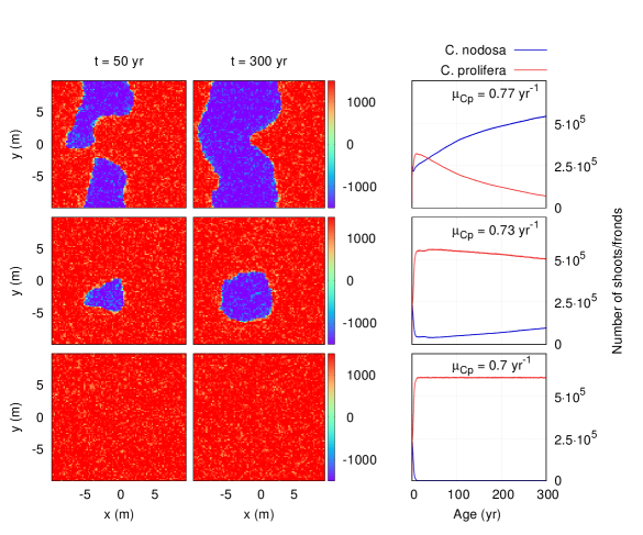
Figure 1: Change in the spatial organization of C. nodosa and C. prolifera in a mixed meadow. The coupling coefficients are $\normalsize\boldsymbol{\gamma_{12}=\gamma_{21}=2}$. The shoot mortality rate for C. nodosa is $\mu_{C_{n}}=0,92\,yr^{-1}$ , whereas the one for C. prolifera changes from $\mu_{C_{p}}=0.77$ to $0.70\,yr^{-1}$, from top to bottom. Different snapshots are taken at $t=50,\,300\,yr$. Regions colored in blue (red) are dominated by the presence of C. nodosa (C. prolifera ), and the color green represents regions of coexistence of both species. The color bar shows the difference between $\rho_{Cp}-\rho_{Cn}$, and it has units of shoots$/m^{2}$. In the right column, the change in the average population of shoots for both species is shown.

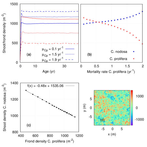
Figure 2: Mixed meadows of C. nodosa and C. prolifera with a coupling coefficient $\normalsize\boldsymbol{\gamma_{12}=\gamma_{21}=0.5}$. (a) Change in the density profile for selected values of $\mu_{C_{p}}$. Red lines: data for C. prolifera; Blue lines: results for C. nodosa. (b) The saturation shoot densities of both species vs $\mu_{C_{p}}$. (c) The shoot density of C. nodosa vs C. prolifera in mixed meadows for different values of $\mu_{C_{p}}$. (d) A snapshot of the meadow taken in the steady state regime at $t=10$ yr. for a C. prolifera mortality rate: $\mu_{C_{p}}=0.65\,yr^{-1}$. The predominance of green color represents a mixed meadow solution. The color bar shows the difference between $\rho_{Cp}-\rho_{Cn}$, and it has units of shoots$/m^{2}$.

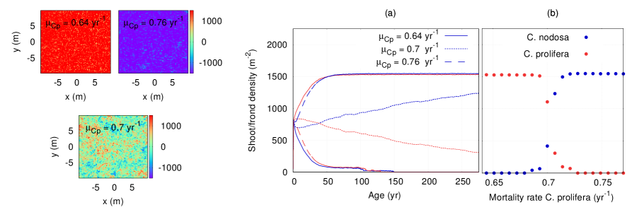
Figure 3: C. nodosa and C. prolifera meadows for coupling coefficients $\normalsize\boldsymbol{\gamma_{12}=\gamma_{21}=1}$. (Left) Snapshots of the three possible states: mono-specific meadows of C. prolifera in red ($\mu_{Cp}=0.64\,yr^{-1}$) or C. nodosa in blue ($\mu_{Cp}=0.76\,yr^{-1}$) (top row), and mixed meadows in green ($\mu_{Cp}=0.70\,yr^{-1}$) (bottom row). The color bar shows the difference between $\rho_{Cp}-\rho_{Cn}$, and it has units of shoot$/m^{2}$. (a) Change in the density profile of both species for selected values of $\mu_{Cp}$. Mixed meadows are found to be a transitory state. (b) Saturation shoot densities for both species vs. $\mu_{Cp}$.

Experimental analysis and model validation

In this section, we study the response of the model to non-symmetric coupling coefficients $\gamma_{12}\neq\gamma_{21}$. One of our main observations is that the results from the symmetric case generalize and the formation of mixed meadows is guaranteed when the coupling coefficients are in the range $0<\gamma_{ij}<1$. In Fig. 4, we plot the shoot densities of C. nodosa ($\rho_{Cn}$) vs. C. prolifera ($\rho_{Cp}$) for different combinations of interaction parameters in $0<\gamma_{ij}<1$. We find that their steady-states are mixed meadow solutions that follow linear relations of the type $\rho_{Cn}={\cal A}\rho_{Cp}+{\cal B}$, as in the symmetric case (Fig. 2(c)). In Fig. 4(a), we kept the mortality of C. nodosa ($\mu_{Cn}$) fixed, while varying the mortality of C. prolifera ($\mu_{Cp}$). Interestingly, we observe that the coupling coefficient $\gamma_{12}$ governs the magnitude of the slope $\cal A$, which follows the relation $\gamma_{12}\sim-\cal A$. We could expect this relation from the linear stability analysis of the model at equilibrium (See Supplementary Materials D). For small values of $\gamma_{12}$, the density $\rho_{Cn}$ is less affected by a change in the mortality $\mu_{Cp}$, resulting in a much smaller slope $\cal A$. Changing the other coefficient $\gamma_{21}$, translates the points along the same line since a decrease in $\gamma_{21}$ favors the growth of C. prolifera at the expense of C. nodosa, and vice-versa. An analogous analysis can be done for Fig. 4(b), where we kept the mortality $\mu_{Cp}$ fixed and varied $\mu_{Cn}$. Here, the coefficient $\gamma_{21}$ controls the slope of the linear regression. In this case, it follows the inverse relation $\gamma_{21}\sim-{\cal A}^{-1}$, and the coefficient $\gamma_{12}$ does not alter the slope.

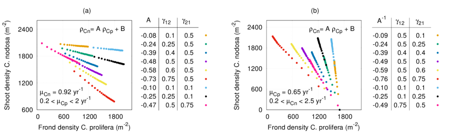
Figure 4: Sensitivity analysis of the model for the coupling parameters: $\gamma_{12},\,\gamma_{21}<1$. We plot the shoot density of C. nodosa vs. C. prolifera in stable mixed meadows. Each color represents a different combination of the coupling coefficients. Each data point corresponds to a different value the C. prolifera mortality rate, $\mu_{Cp}$, in (a), and the C. nodosa mortality rate, $\mu_{Cn}$, in (b). The different sets of points fit the linear regressions of slope $A$, with an error not higher than $2\%$ in any of the cases.

After the analysis of the model behavior, it is possible to determine the coupling coefficients $\gamma_{ij}$ in real meadows by comparing the results of our simulations with the experimental data. We measured the averaged shoot density in meadows of C. nodosa and C. prolifera in 106 sampling points in the Alfacs Bay (Ebro River Delta - Spain), shown with purple dots in Figure 5. The presence of mixed meadows of these two species indicates values of the couplings $\gamma_{12},\,\gamma_{21}<1$. Although data is highly scattered, it is possible to find linear relationships between the shoot densities of C. nodosa, vs. C. prolifera: $\rho_{Cn}={\cal A}\rho_{Cp}+{\cal B}$. We use the least-square method to fit the data [Watson, 1967]. This method minimizes the errors of one of the data sets and considers the other as a control variable with no error. If we choose to minimize the errors in the measurements of $\rho_{Cn}$, the best fit to the data gives a slope of ${\cal A}=-0.47\pm 0.11$ (solid blue line). This slope, within its error, is in a very good agreement with the model outcome for $\gamma_{12}\sim 0.5$ according to Fig. 4(a). The linear regression that minimizes the errors in $\rho_{Cp}$ has a slope of ${\cal A}=-3.3\pm 0.7$ (solid red line), which coincides with the simulations when $\gamma_{21}\sim 0.3$ (Fig. 4(b)). Therefore, the numerical model nicely reproduces field data for $\gamma_{12}=0.5$ and $\gamma_{21}=0.3$. For these coupling coefficients, the simulations with fixed $\mu_{Cn}$ and varying $\mu_{Cp}$ generate the dotted blue line, and similarly for the dotted red line, by keeping $\mu_{Cp}$ constant and mo $\mu_{Cn}$. The match between model and data is one of our main results, which establishes $\gamma_{ij}$ as the key parameter to allow the connection between the numerical model and the experimental data and provide information on the strength of the interaction between species.

Figure 5: Comparison between the model outcome and the experimental data. The purple dots correspond to experimental measurements of shoot densities of C. nodosa and C. prolifera in mixed meadows in the Alfacs Bay (Ebro River Delta, Spain). The solid lines correspond to two types of linear fits of the experimental data, minimizing both the errors in the measurements of density of C. nodosa (solid blue line), or minimizing the errors in C. prolifera (solid red line). The dotted lines are the results of our simulations assuming coupling parameters $\normalsize\boldsymbol{\gamma_{12}=0.5$,\,$\gamma_{21}=0.3}$. The dotted blue line is reproduced by keeping the mortality of C. nodosa fixed, while varying the mortality C. prolifera, and vice-versa for the dotted red line. For a better comparison with the field measurements, the maximum shoot density has been adjusted to the average values found in the Alfacs Bay location ($\rho_{max,Cn}=2300\,m^{-2}$ and $\rho_{max,Cp}=1900\,m^{-2}$).

In all previous studies we assumed an initial condition consisting of a mixed meadow with the same amount of seeds of both species homogeneously distributed all over the available space. We analyze the sensitivity of the results to the initial condition. We will assume the case in which patches of different species are initially placed apart from each other. In a square region of size $L^{2}=40\times 40\,m^{2}$, we locate a homogeneous density of seeds along two vertical stripes, $1\,m$ wide, one of C. nodosa, centered at $x=-10\,m$, and another of C. prolifera, centered at $x=10\,m$ (Figure 6 ($t=0\,yr$)). During a short period of time, two separated mono-specific meadows develop. Shortly after that, the two domains collide forming a clear front (Figure 6 ($t\sim 8\,yr$)). At this stage, the two species have reached their maximum shoot density values. This front quickly dilutes giving rise to a mixed meadow of C. prolifera and C. nodosa (Figure 6 ($t\sim 19\,yr$)). The final state of the system is comparable to that collected assuming a homogeneous initial distribution of seeds (see Figure 2(d)).

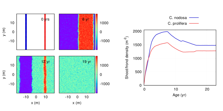
Figure 6: (Left) Spatial distribution, at different time steps, of two competing species: C. nodosa (blue) and C. prolifera (red), starting from two well defined striped patches separated from each other. As time evolves, both species cover all available space forming a mixed meadow (green). The color bar shows the difference between $\rho_{Cp}-\rho_{Cn}$, and it has units of shoots$/m^{2}$. (Right) Evolution of the averaged density of both species. The interaction coefficients are set to $\gamma_{12}=0.5$ and $\gamma_{21}=0.3$, and the mortality rates, $\mu_{Cp}=0.65\,yr^{-1}$, and $\mu_{Cn}=0.92\,yr^{-1}$.

DISCUSSION

In this paper we present the results of an agent-based model that investigates the dynamics of growth of clonal organisms (like seagrasses and seaweeds) in a scenario of species competition. The interaction among species has been implemented through a coupling parameter, $\gamma_{ij}$, placed in the local interaction term (eq. (2)) that quantifies the strength of the interaction between any pair of species. We found the value of this coupling parameter to determine the model outcome that ranges from separated and well defined mono-specific domains to mixed ones. A comparison between the model outcome and field measurements, conducted in the Alfacs Bay where large meadows of C. nodosa and C. prolifera are present, allowed us to determine the coupling coefficients between these two species ($\gamma_{12}=0.5$, $\gamma_{21}=0.3$) and it is one of the main findings of this paper (Fig. 5). In our simulations, the choice of coupling parameters $\gamma_{ij}$ is decisive since they reflect the type and magnitude of the interaction between species: $\gamma_{12}$ controls the influence of C. prolifera over C. nodosa, and vice-versa for $\gamma_{21}$. The asymmetry found in the results is a clear indication that the negative effect of the presence of C. prolifera over C. nodosa is higher than vice-versa. The fact that both coefficients are in the $\gamma_{ij}<1$ regime implies that the seagrass/seaweed competes less with the shoots of the other species than with their own. Therefore, in order to minimize the competition, species self-organize and form mixed meadows. This effect should typically be explained by several biologically relevant mechanisms related to the anatomy, metabolism, or other properties of the plants. Although C. prolifera and C. nodosa have comparable magnitudes in their clonal growth rates (Supplementary Materials A), they have very different root lengths: while C. nodosa extends into the sediment to a mean depth of $14.1cm$, the roots of C. prolifera just elongate an average of $3cm$ [Duarte et al., 1998, Bedinger et al., 2013]. This characteristic allows the shoots of the two species to absorb the nutrients from different soil regions, making self-competition higher than the interspecific competition, favoring the appearance of mixed meadows. Therefore, our numerical analysis leads us to conjecture that the difference in root lengths between species is one of the main mechanisms that mediate the formation of mixed meadows of C. nodosa and C. prolifera.

Our analysis is consistent with previous results found in the literature. In [Tuya et al., 2013], shoot densities in mixed meadows of C. nodosa and C. prolifera were collected in 16 sites across Gran Canaria island (Spain, Atlantic Ocean) in the summer season, when the meadows should be at their optimal growth. The best linear fit to their data ($\rho_{1}={\cal A}\rho_{2}+{\cal B}$), minimizing the errors in the measurements of C. nodosa, led to a slope ${\cal A}=-0.71\pm 0.35$ which is consistent with our findings (Fig. 5). Despite the similarities found, different slopes can be expected due to the very different conditions between the locations of both experiments: the sites in our experiment were located in the Ebro River Delta, that is characterized by very calm, shallow, and high-on-nutrient waters, while sites in [Tuya et al., 2013] were in Gran Canary island, whose coastline has a lack of pronounced geographical accidents and it is very exposed to winds and currents.

In [Tuya et al., 2013], they also performed an experiment to establish the direct effect of C. prolifera over C. nodosa. In mixed meadows, $100\%$ of the fronds of C. prolifera were removed. Eight months later, the density of shoots of C. nodosa increased $1.5$-times. This result is also consistent with our findings. When the two species are allowed to grow separately, setting appropiate initial conditions as those depicted in Fig. 6, C. nodosa patches reach a maximum density of $\rho_{Cn}=2000\,m^{-2}$ (maximum of the solid blue line at $t\sim 8\,yr$). Once the two species meet and interact a stable mixed meadow of C. prolifera and C. nodosa develop with densities $\rho_{Cn}=1480\,m^{-2}$ and $\rho_{Cp}=1270\,m^{-2}$. Thus, isolated meadows of C. nodosa have an average shoot density $1.35$-times higher that in mixed meadows. Therefore, our model supports the observations made in [Tuya et al., 2013], where they conclude that the appearance of C. prolifera partially contributes to the demise of the population of C. nodosa. Also in [Pérez-Ruzafa et al., 2012], the changes of seagrass beds in Mar Menor Coastal Lagoon (Spain, Mediterranean Sea) were analyzed. They observed a decrease and almost total loss of C. nodosa in deeper areas of the lagoon ($2-7m$) after a colonization event of C. prolifera in the early 1970’s. Our simulations sustain the hypothesis that the invasion of C. prolifera should negatively influence the abundance of C. nodosa. Still, this cannot solely explain the loss of C. nodosa, and we should consider other effects that deteriorate the seagrass. For example, light availability could be a key effect in the dynamics of C. nodosa and C. prolifera meadows, since it affects both species very differently. While C. prolifera suffers from photoinhibition in transparent shallow areas, the shoot density of C. nodosa could be limited by an increased content of silt, clay, organic matter, or phytoplankton[Pérez-Ruzafa et al., 2012, Pérez-Ruzafa et al., 2019, García-Sánchez et al., 2012]. In [Belando et al., 2021], the most recent study of the distribution of C. nodosa and C. prolifera in the Mar Menor, they study the presence of mixed meadows in the deeper areas of the lagoon (less than $-4m$). Their data does not show a negative correlation between the biomass of both macrophytes, which is in disagreement with our findings in Fig. 5. The discrepancy between both observations might be related to the different environmental conditions among study sites, and it should be further investigated.

In this work, we have presented the first numerical model that studies local interactions among different species of rhizomatous macrophytes. Although the present work has focused on mixed meadows of C. nodosa and C. prolifera, the proposed model can be applied to study the interactions between generic $N$-species. For example, by properly adjusting the clonal growth parameters and coupling coefficients, we could simulate the dynamics of tropical seagrass beds, with a large diversity of coexisting species [Short et al., 2007]. Also, this numerical model can be used to predict the re-distribution of seagrasses over the ocean floor due to global warming, paying special attention to the competition between species with different thermal thresholds, such as P. oceanica and C. nodosa, or the role of invasive species [Savva et al., 2018, Rius et al., 2014]. Finally, this work sets the necessary framework to study long-range interactions between seagrass species. These types of interactions are often mediated by chemical concentrations and are responsible for the appearance of optimal sea-scape patterns [Ruiz-Reynés et al., 2017]. In future work, we will extend the current model to consider such effects.

AUTHORSHIP

NM, EM, ELL, and TS conceived this study. ELL developed the models, produced the figures, and analyzed the data. EM carried out the field observations, and wrote the experimental methodology section. NM, EM, ELL, and TS analized the results. ELL wrote the initial draft and all coauthors contributed to editing the manuscript.

References

- [Alós et al., 2016] Alós, J., Tomas, F., Terrados, J., Verbruggen, H., and Ballesteros, E. (2016). Fast-spreading green beds of recently introduced halimeda incrassata invade mallorca island (NW mediterranean sea). Marine Ecology Progress Series, 558:153–158.
- [Arnaud-Haond et al., 2012] Arnaud-Haond, S., Duarte, C. M., Diaz-Almela, E., Marbà, N., Sintes, T., and Serrão, E. A. (2012). Implications of extreme life span in clonal organisms: Millenary clones in meadows of the threatened seagrass posidonia oceanica. PLoS ONE, 7(2):e30454.
- [Bedinger et al., 2013] Bedinger, L. A., Bell, S. S., and Dawes, C. J. (2013). Rhizophytic algal communities of shallow, coastal habitats in florida: Components above and below the sediment surface. Bulletin of Marine Science, 89(2):437–460.
- [Belando et al., 2021] Belando, M., Bernardeau-Esteller, J., Paradinas, I., Ramos-Segura, A., García-Muñoz, R., García-Moreno, P., Marín-Guirao, L., and Ruiz, J. M. (2021). Long-term coexistence between the macroalga caulerpa prolifera and the seagrass cymodocea nodosa in a mediterranean lagoon. Aquatic Botany, 173:103415.
- [Bell and Tomlinson, 1980] Bell, A. D. and Tomlinson, P. B. (1980). Adaptive architecture in rhizomatous plants. Botanical Journal of the Linnean Society, 80(2):125–160.
- [Bonacorsi et al., 2013] Bonacorsi, M., Pergent-Martini, C., Breand, N., and Pergent, G. (2013). Is posidonia oceanica regression a general feature in the mediterranean sea? Mediterranean Marine Science, 14(1):193–203.
- [Borum et al., 2013] Borum, J., Raun, A. L., Hasler-Sheetal, H., Pedersen, M. O., Pedersen, O., and Holmer, M. (2013). Eelgrass fairy rings: sulfide as inhibiting agent. Marine Biology, 161(2):351–358.
- [Collier et al., 2011] Collier, C. J., Uthicke, S., and Waycott, M. (2011). Thermal tolerance of two seagrass species at contrasting light levels: Implications for future distribution in the great barrier reef. Limnology and Oceanography, 56(6):2200–2210.
- [Costanza et al., 1997] Costanza, R., d’Arge, R., de Groot, R., Farber, S., Grasso, M., Hannon, B., Limburg, K., Naeem, S., O’Neill, R. V., Paruelo, J., Raskin, R. G., Sutton, P., and van den Belt, M. (1997). The value of the world’s ecosystem services and natural capital. Nature, 387(6630):253–260.
- [de Villèle and Verlaque, 1995] de Villèle, X. and Verlaque, M. (1995). Changes and degradation in a posidonia oceanica bed invaded by the introduced tropical alga caulerpa taxifolia in the north western mediterranean. Botanica Marina, 38(1-6).
- [Duarte, 1989] Duarte, C. (1989). Temporal biomass variability and production/biomass relationships of seagrass communities. Marine Ecology Progress Series, 51:269–276.
- [Duarte et al., 1994] Duarte, C., Marbá, N., Agawin, N., Cebrián, J., Enriquez, S., Fortes, M., Gallegos, M., Merino, M., Olesen, B., Sand-Jensen, K., Uri, J., and Vermaat, J. (1994). Reconstruction of seagrass dynamics: age determinations and associated tools for the seagrass ecologist. Marine Ecology Progress Series, 107:195–209.
- [Duarte et al., 1998] Duarte, C., Merino, M., Agawin, N., Uri, J., Fortes, M., Gallegos, M., Marbá, N., and Hemminga, M. (1998). Root production and belowground seagrass biomass. Marine Ecology Progress Series, 171:97–108.
- [Duarte et al., 2005] Duarte, C. M., Middelburg, J. J., and Caraco, N. (2005). Major role of marine vegetation on the oceanic carbon cycle. Biogeosciences, 2(1):1–8.
- [Duarte et al., 2013] Duarte, C. M., Sintes, T., and Marbà, N. (2013). Assessing the co2 capture potential of seagrass restoration projects. Journal of Applied Ecology, 50(6):1341–1349.
- [Fonseca and Cahalan, 1992] Fonseca, M. S. and Cahalan, J. A. (1992). A preliminary evaluation of wave attenuation by four species of seagrass. Estuarine, Coastal and Shelf Science, 35(6):565–576.
- [Frederiksen et al., 2004] Frederiksen, M., Krause-Jensen, D., Holmer, M., and Laursen, J. S. (2004). Spatial and temporal variation in eelgrass (zostera marina) landscapes: influence of physical setting. Aquatic Botany, 78(2):147–165.
- [García-Sánchez et al., 2012] García-Sánchez, M., Korbee, N., Pérez-Ruzafa, I. M., Marcos, C., Domínguez, B., Figueroa, F. L., and Pérez-Ruzafa, Á. (2012). Physiological response and photoacclimation capacity of caulerpa prolifera (forsskål) j.v. lamouroux and cymodocea nodosa (ucria) ascherson meadows in the mar menor lagoon (se spain). Marine Environmental Research, 79:37–47.
- [Hughes et al., 2009] Hughes, A. R., Williams, S. L., Duarte, C. M., Heck, K. L., and Waycott, M. (2009). Associations of concern: declining seagrasses and threatened dependent species. Frontiers in Ecology and the Environment, 7(5):242–246.
- [Invers et al., 1997] Invers, O., Romero, J., and Pérez, M. (1997). Effects of ph on seagrass photosynthesis: a laboratory and field assessment. Aquatic Botany, 59:185–194.
- [Marbà and Duarte, 1998] Marbà, N. and Duarte, C. M. (1998). Rhizome elongation and seagrass clonal growth. Marine Ecology Progress Series, 174:269–280.
- [Mascaró et al., 2014] Mascaró, O., Romero, J., and Pérez, M. (2014). Seasonal uncoupling of demographic processes in a marine clonal plant. Estuarine Coastal and Shelf Science, 142:23–31.
- [Norton, 1976] Norton, T. (1976). Why is sargassum muticum so invasive. British phycological journal, 11:197–198.
- [Orth et al., 2006] Orth, R., Carruthers, T., Dennison, W., Duarte, C., Fourqurean, J., Heck, K., Hughes, A., Kendrick, G., Kenworthy, W., Olyarnik, S., Short, F., Waycott, M., and Williams, S. (2006). A global crisis for seagrass ecosystems. BioScience, 56(12):987–996.
- [Pasqualini et al., 1999] Pasqualini, V., Pergent-Martini, C., and Pergent, G. (1999). Environmental impact identification along the corsican coast (mediterranean sea) using image processing. Aquatic Botany, 65:311–320.
- [Pérez et al., 1994] Pérez, M., Duarte, C. M., Romero, J., Sand-Jensen, K., and Alcoverro, T. (1994). Growth plasticity in cymodocea nodosa stands: the importance of nutrient supply. Aquatic Botany, 47(3):249–264.
- [Pérez et al., 2001] Pérez, M., Mateo, M. A., Alcoverro, T., and Romero, J. (2001). Variability in detritus stocks in beds of the seagrass cymodocea nodosa. Botanica Marina, 44(6):523–531.
- [Pérez-Ruzafa et al., 2019] Pérez-Ruzafa, A., Campillo, S., Fernández-Palacios, J. M., García-Lacunza, A., García-Oliva, M., Ibañez, H., Navarro-Martínez, P. C., Pérez-Marcos, M., Pérez-Ruzafa, I. M., Quispe-Becerra, J. I., Sala-Mirete, A., Sánchez, O., and Marcos, C. (2019). Long-term dynamic in nutrients, chlorophyll a, and water quality parameters in a coastal lagoon during a process of eutrophication for decades, a sudden break and a relatively rapid recovery. Frontiers in Marine Science, 6.
- [Pérez-Ruzafa et al., 2012] Pérez-Ruzafa, A., Marcos, C., Bernal, C. M., Quintino, V., Freitas, R., Rodrigues, A. M., García-Sánchez, M., and Pérez-Ruzafa, I. M. (2012). Cymodocea nodosa vs. caulerpa prolifera: Causes and consequences of a long term history of interaction in macrophyte meadows in the mar menor coastal lagoon (spain, southwestern mediterranean). Estuarine, Coastal and Shelf Science, 110:101–115. Coastal Lagoons in a changing environment: understanding, evaluating and responding.
- [Rius et al., 2014] Rius, M., Clusella-Trullas, S., McQuaid, C. D., Navarro, R. A., Griffiths, C. L., Matthee, C. A., von der Heyden, S., and Turon, X. (2014). Range expansions across ecoregions: interactions of climate change, physiology and genetic diversity. Global Ecology and Biogeography, 23(1):76–88.
- [Ruiz-Reynés and Gomila, 2019] Ruiz-Reynés, D. and Gomila, D. (2019). Distribution of growth directions in meadows of clonal plants. Physical Review E, 100(5).
- [Ruiz-Reynés et al., 2017] Ruiz-Reynés, D., Gomila, D., Sintes, T., Hernández-García, E., Marbà, N., and Duarte, C. (2017). Fairy circle landscapes under the sea. Science Advances, 3(8).
- [Ruiz-Reynés et al., 2020] Ruiz-Reynés, D., Martín, L., Hernández-García, E., Knobloch, E., and Gomila, D. (2020). Patterns, localized structures and fronts in a reduced model of clonal plant growth. Physica D: Nonlinear Phenomena, 414:132723.
- [Sánchez-González et al., 2011] Sánchez-González, J. F., Sánchez-Rojas, V., and Memos, C. D. (2011). Wave attenuation due toPosidonia oceanicameadows. Journal of Hydraulic Research, 49(4):503–514.
- [Savva et al., 2018] Savva, I., Bennett, S., Roca, G., Jordà, G., and Marbà, N. (2018). Thermal tolerance of mediterranean marine macrophytes: Vulnerability to global warming. Ecology and Evolution, 8(23):12032–12043.
- [Short et al., 2007] Short, F., Carruthers, T., Dennison, W., and Waycott, M. (2007). Global seagrass distribution and diversity: A bioregional model. Journal of Experimental Marine Biology and Ecology, 350(1):3–20. The Biology and Ecology of Seagrasses.
- [Sintes et al., 2006] Sintes, T., Marbà, N., and Duarte, C. M. (2006). Modeling nonlinear seagrass clonal growth: Assessing the efficiency of space occupation across the seagrass flora. Estuaries and Coasts, 29(1):72–80.
- [Sintes et al., 2005] Sintes, T., Marbà, N., Duarte, C. M., and Kendrick, G. A. (2005). Nonlinear processes in seagrass colonisation explained by simple clonal growth rules. Oikos, 108(1):165–175.
- [Tuya et al., 2013] Tuya, F., Hernandez-Zerpa, H., Espino, F., and Haroun, R. (2013). Drastic decadal decline of the seagrass cymodocea nodosa at gran canaria (eastern atlantic): Interactions with the green algae caulerpa prolifera. Aquatic Botany, 105:1–6.
- [van der Heide et al., 2010] van der Heide, T., Bouma, T. J., van Nes, E. H., van de Koppel, J., Scheffer, M., Roelofs, J. G. M., van Katwijk, M. M., and Smolders, A. J. P. (2010). Spatial self-organized patterning in seagrasses along a depth gradient of an intertidal ecosystem. Ecology, 91(2):362–369.
- [Vergés et al., 2014] Vergés, A., Steinberg, P. D., Hay, M. E., Poore, A. G. B., Campbell, A. H., Ballesteros, E., Heck, K. L., Booth, D. J., Coleman, M. A., Feary, D. A., Figueira, W., Langlois, T., Marzinelli, E. M., Mizerek, T., Mumby, P. J., Nakamura, Y., Roughan, M., van Sebille, E., Gupta, A. S., Smale, D. A., Tomas, F., Wernberg, T., and Wilson, S. K. (2014). The tropicalization of temperate marine ecosystems: climate-mediated changes in herbivory and community phase shifts. Proceedings of the Royal Society B: Biological Sciences, 281(1789):20140846.
- [Watson, 1967] Watson, G. S. (1967). Linear least squares regression. The Annals of Mathematical Statistics, 38(6):1679–1699.
- [Watson et al., 1993] Watson, R., Coles, R., and Long, W. L. (1993). Simulation estimates of annual yield and landed value for commercial penaeid prawns from a tropical seagrass habitat, northern queensland, australia. Marine and Freshwater Research, 44(1):211.
- [Waycott et al., 2009] Waycott, M., Duarte, C., Carruthers, T., Orth, R., Dennison, W., Olyarnik, S., Calladine, A., Fourqurean, J., Heck, K., Hughes, A., Kendrick, G., Kenworthy, W., Short, F., and Williams, S. (2009). Accelerating loss of seagrasses across the globe threatens coastal ecosystems. PNAS; Proceedings of the National Academy of Sciences, 106(30):12377–12381.
- [Wesselmann et al., 2021] Wesselmann, M., Chefaoui, R. M., Marbà, N., Serrao, E. A., and Duarte, C. M. (2021). Warming threatens to propel the expansion of the exotic seagrass halophila stipulacea. Frontiers in Marine Science, 8.