Adversarial Attack and Defense for Non-Parametric Two-Sample Tests

Abstract

Non-parametric two-sample tests (TSTs) that judge whether two sets of samples are drawn from the same distribution, have been widely used in the analysis of critical data. People tend to employ TSTs as trusted basic tools and rarely have any doubt about their reliability. This paper systematically uncovers the failure mode of non-parametric TSTs through adversarial attacks and then proposes corresponding defense strategies. First, we theoretically show that an adversary can upper-bound the distributional shift which guarantees the attack’s invisibility. Furthermore, we theoretically find that the adversary can also degrade the lower bound of a TST’s test power, which enables us to iteratively minimize the test criterion in order to search for adversarial pairs. To enable TST-agnostic attacks, we propose an ensemble attack (EA) framework that jointly minimizes the different types of test criteria. Second, to robustify TSTs, we propose a max-min optimization that iteratively generates adversarial pairs to train the deep kernels. Extensive experiments on both simulated and real-world datasets validate the adversarial vulnerabilities of non-parametric TSTs and the effectiveness of our proposed defense. Source code is available at https://github.com/GodXuxilie/Robust-TST.git.

1 Introduction

Non-parametric two-sample tests (TSTs) that judge whether two sets of samples drawn from the same distribution have been widely used to analyze critical data in physics (baldi2014searching), neurophysiology (rasch2008predicting), biology (borgwardt2006integrating), etc. Compared with traditional methods (such as the t-test), non-parametric TSTs can relax the strong parametric assumption about the distributions being studied and are effective in complex domains (gretton2009fast; gretton2012kernel; chwialkowski2015fast; jitkrittum2016interpretable; sutherland2016generative; lopez2016revisiting; cheng2019classification; liu2020learning; liu2021meta). Notably, the use of deep kernels (liu2020learning) flexibly empowers the non-parametric TSTs to learn even more complex distributions.

However, the adversarial robustness of non-parametric TSTs is rarely studied, despite its extensive studies for deep neural networks (DNNs). Studies of DNNs’ adversarial robustness (Madry_adversarial_training) have enabled significant advances in defending against adversarial attacks (szegedy), which can help enhance the security in various domains such as computer vision (xie2017adversarial; mahmood2021robustness), natural language processing (Zhu2020FreeLB:; yoo2021towards), recommendation system (peng2020robust), etc. We therefore undertake this pioneer study on adversarial robustness of non-parametric TSTs, which uncovers the failure mode of non-parametric TSTs through adversarial attacks and facilitate an effective strategy for making TSTs reliable in critical applications (baldi2014searching; rasch2008predicting; borgwardt2006integrating).

First, we theoretically show the adversary could upper-bound the distributional shift and degrade the lower bound of a TST’s test power (details in Section 3.1). Given a benign pair $(S_{\mathbb{P}},S_{\mathbb{Q}})$, in which $S_{\mathbb{P}}=\{{x}_{i}\}_{i=1}^{m}\sim\mathbb{P}^{m}$ and $S_{\mathbb{Q}}=\{{y}_{j}\}_{j=1}^{n}\sim\mathbb{Q}^{n}$ , an $\ell_{\infty}$-bounded adversary could generate the adversarial pair $(S_{\mathbb{P}},\tilde{S}_{\mathbb{Q}})$. We will show in Proposition 1 that the maximum mean discrepancy (MMD) (gretton2012kernel) between the benign and adversarial pairs is upper-bounded, which guarantees imperceptible adversarial perturbations (szegedy). Furthermore, we will show in Theorem LABEL:theory:tp_attack that the adversary can degrade the lower bound of a TST’s test power, which implies that a TST could wrongly determine $\mathbb{P}=\mathbb{Q}$ with a larger probability under adversarial attacks when $\mathbb{P}\neq\mathbb{Q}$ holds.

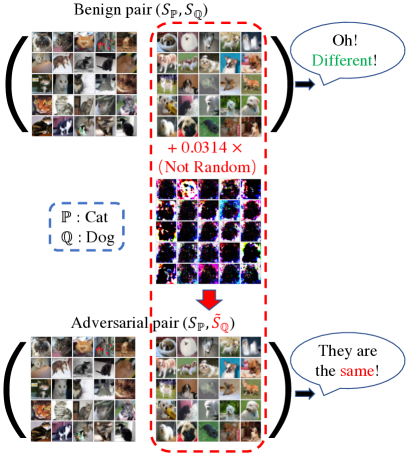
Figure 1: An example of adversarial pair $(S_{\mathbb{P}},\tilde{S}_{\mathbb{Q}})$ generated by embedding an adversarial perturbation in the benign set $S_{\mathbb{Q}}$ of the benign pair $(S_{\mathbb{P}},S_{\mathbb{Q}})$. Experimental details are in Section LABEL:sec:attack_power.

Then, we realize effective adversarial attacks against non-parametric TSTs (details in Section LABEL:sec:realization). We formulate an attack as a constraint optimization problem that minimizes a TST’s test criterion (liu2020learning) within the $\ell_{\infty}$-bound of size $\epsilon$ on $S_{\mathbb{Q}}$. We utilize projected gradient descent (PGD) (Madry_adversarial_training) to efficiently search the adversarial set $\tilde{S}_{\mathbb{Q}}$ and incorporate automatic schedule of the step size (croce2020reliable) to improve the optimization convergence. Moreover, we extend the attack beyond a specific TST to a generic TST-agnostic attack, namely, ensemble attack (EA). EA jointly minimizes a weighted sum of different test criteria, which can simultaneously fool various TSTs. For example, Figure 1 shows non-parametric TSTs can correctly differentiate the benign pair of “cats” and “dogs” (top) coming from the different distributions, but wrongly judge adversarial pairs (bottom) as belonging to the same distribution.

Second, to robustify the non-parametric TSTs, we study the corresponding defense approaches (details in Section LABEL:sec:defense). A straightforward defense seems to use an ensemble of TSTs. We find an ensemble of TSTs is sometimes effective against a specific attack targeting a certain type of TSTs but almost always fails under EA (see experiments in Section LABEL:sec:attack_power). Therefore, to effectively defend against adversarial attacks, we propose to adversarially learn the robust kernels. The defense is formulated as a max-min optimization that is similar in flavor to the adversarial training’s min-max formulation (Madry_adversarial_training). For its realization, we iteratively generate adversarial pairs by minimizing the test criterion in the inner minimization and update kernel parameters by maximizing the test criterion on the adversarial pairs in the outer maximization. We realize our defense using deep kernels that have achieved the state-of-the-art (SOTA) performance in non-parametric TSTs (liu2020learning).

Lastly, we empirically justify the proposed attacks and defenses (in Section LABEL:sec:exp). We evaluate the test power of many existing non-parametric TSTs (non-robust) and the robust-kernel TST (robust) under the EA on simulated and real-world datasets, including complex synthetic distributions, high-energy physics data, and challenging images. Comprehensive experimental results validate that the existing non-parametric TSTs lack adversarial robustness; we can significantly improve the adversarial robustness of non-parametric TSTs through adversarially learning the deep kernels.

2 Non-Parametric Two-Sample Tests

In this section, we provide the preliminaries of non-parametric TSTs and provide discussions with the related studies in Appendix LABEL:sec:related_work.

2.1 Problem Formulation

Let $\mathcal{X}\subset\mathbb{R}^{d}$ and $\mathbb{P}$, $\mathbb{Q}$ be Borel probability measures on $\mathcal{X}$. A non-parametric TST $\mathcal{J}(S_{\mathbb{P}},S_{\mathbb{Q}}):\mathcal{X}^{m}\times\mathcal{X}^{n}\mapsto\{0,1\}$ is used to distinguish between the null hypothesis $\mathcal{H}_{0}:\mathbb{P}=\mathbb{Q}$ and the alternative hypothesis $\mathcal{H}_{1}:\mathbb{P}\neq\mathbb{Q}$, where $S_{\mathbb{P}}$ and $S_{\mathbb{Q}}$ are independent identically distributed (IID) samples of size $m$ and $n$ drawn from $\mathbb{P}$ and $\mathbb{Q}$, respectively. A non-parametric TST constructs a mean embedding based on a kernel parameterized with $\theta$ for each distribution, and utilizes the differences in these embeddings as the test statistic for the hypothesis test. The judgement is made by comparing the test statistic $\mathcal{D}(S_{\mathbb{P}},S_{\mathbb{Q}})$ with a particular threshold $r$: if the threshold is exceeded, then the test rejects $\mathcal{H}_{0}$. The test power (TP) of a non-parametric TST $\mathcal{J}$ is measured by the probability of correctly rejecting $\mathcal{H}_{0}$ when the alternative hypothesis is true, i.e., $\mathrm{TP}(\mathcal{J})=\mathbb{E}_{S_{\mathbb{P}}\sim\mathbb{P}^{m},S_{\mathbb{Q}}\sim\mathbb{Q}^{n}}[\mathbbm{1}(\mathcal{J}(S_{\mathbb{P}},S_{\mathbb{Q}})=1)]$ for a paritular $\mathbb{P}\neq\mathbb{Q}$. A non-parametric TST optimizes its learnable parameters $\theta$ via maximizing its test criterion, thus approximately maximizing its test power.

2.2 Test Statistics

Here, we introduce a typical test statistic, maximum mean discrepancy (MMD) (gretton2012kernel), and leave other test statistics in Appendix LABEL:appendix:tst_intro, such as tests based on Gaussian kernel mean embeddings at specific positions (chwialkowski2015fast; jitkrittum2016interpretable) and classifier two-sample tests (C2ST) (lopez2016revisiting; cheng2019classification).

Definition 1 (gretton2012kernel).

Let $k:\mathcal{X}\times\mathcal{X}\to\mathbb{R}$ be a kernel of a reproducing kernel Hilbert space $\mathcal{H}_{k}$, with feature maps $k(\cdot,x)\in\mathcal{H}_{k}$. Let $X\sim\mathbb{P}$ and $Y\sim\mathbb{Q}$, and define the kernel mean embeddings $\mu_{\mathbb{P}}=\mathbb{E}[k(\cdot,X)]$ and $\mu_{\mathbb{Q}}=\mathbb{E}[k(\cdot,Y)]$. Under mild integrability conditions,

$$\mathrm{MMD}(\mathbb{P},\mathbb{Q};\mathcal{H}_{k}) =\sup_{f\in\mathcal{H},\|f\|_{\mathcal{H}_{k}}\leq 1}|\mathbb{E}[f(X)]-\mathbb{E}[f(Y)]|$$

$$=\|\mu_{\mathbb{P}}-\mu_{\mathbb{Q}}\|_{\mathcal{H}_{k}}.$$ (1)

For characteristic kernels, $\mathrm{MMD}(\mathbb{P},\mathbb{Q};\mathcal{H}_{k})=0$ if and only if $\mathbb{P}=\mathbb{Q}$. Assuming $n=m$, we can estimate $\mathrm{MMD}$ (Eq. (1)) using the $U$-statistic estimator, which is unbiased for ${\mathrm{MMD}}^{2}$ and has nearly minimal variance among all unbiased estimators (gretton2012kernel):

$${\widehat{\mathrm{MMD}}}^{2}(S_{\mathbb{P}},S_{\mathbb{Q}};k)=\frac{1}{n(n-1)}\sum_{i\neq j}H_{ij},$$ (2)

$$H_{ij} =k(x_{i},x_{j})+k(y_{i},y_{j})-k(x_{i},y_{j})-k(x_{j},y_{i}),$$

where $x_{i},x_{j}\in S_{\mathbb{P}}$ and $y_{i},y_{j}\in S_{\mathbb{Q}}$.

In this paper, we investigate six types of non-parametric TSTs as follows since liu2020learning; liu2021meta have shown they are powerful on complex data.

• $\mathcal{D}^{(\mathrm{G})}(\cdot,\cdot;k^{(\mathrm{G})})={\widehat{\mathrm{MMD}}}^{2}(\cdot,\cdot;k^{(\mathrm{G})})$ for tests based on MMD with Gaussian kernels (MMD-G) (sutherland2016generative) with the learnable lengthscale $\sigma_{\phi}$, in which $k^{(\mathrm{G})}(x,y)=\exp(-\frac{1}{2\sigma_{\phi}}\|x-y\|^{2})$.

• $\mathcal{D}^{(\mathrm{D})}(\cdot,\cdot;k^{(\mathrm{D})})={\widehat{\mathrm{MMD}}}^{2}(\cdot,\cdot;k^{(\mathrm{D})})$ for tests based on MMD with deep kernels (MMD-D) (liu2020learning). Note that $k^{(\mathrm{D})}(x,y)=[(1-\gamma)\exp(-\frac{1}{2\sigma_{\phi}}\|\phi(x)-\phi(y)\|^{2})+\gamma]\exp(-\frac{1}{2\sigma_{q}}\|x-y\|^{2})$ where $\gamma,\sigma_{\phi},\sigma_{q}$ are the learnable parameters and $\phi(\cdot)$ is a parameterized deep network to extract the features.

• $\mathcal{D}^{(\mathrm{S})}(\cdot,\cdot)$ (Eq. (LABEL:eq:ts_c2sts)) for C2ST based on Sign (C2ST-S) (lopez2016revisiting). A classifier $f:\mathcal{X}\rightarrow\mathbb{R}$ that outputs the classification probabilities is utilized by C2ST. liu2020learning pointed out that the test statistic of C2ST-S is equivalent to MMD with kernel $k^{(\mathrm{S})}$, i.e., $\mathcal{D}^{(\mathrm{S})}(\cdot,\cdot)={\widehat{\mathrm{MMD}}}^{2}(\cdot,\cdot;k^{(\mathrm{S})})$ where $k^{(\mathrm{S})}(x,y)=\frac{1}{4}\mathbbm{1}(f(x)>0)\mathbbm{1}(f(y)>0)$.

• $\mathcal{D}^{(\mathrm{L})}(\cdot,\cdot)$ (Eq. (LABEL:eq:ts_s2stl)) for C2ST-L (cheng2019classification) that utilizes the discriminator’s measure of confidence. Its test statistic is also equivalent to MMD with kernel $k^{(\mathrm{L})}$ (liu2020learning), i.e., $\mathcal{D}^{(\mathrm{L})}(\cdot,\cdot)={\widehat{\mathrm{MMD}}}^{2}(\cdot,\cdot;k^{(\mathrm{L})})$ where $k^{(\mathrm{L})}(x,y)=f(x)f(y)$.

• $D^{(\mathrm{ME})}(\cdot,\cdot)$ (Eq. (LABEL:eq:ts_ME)) for tests based on differences in Gaussian kernel mean embeddings at specific locations (chwialkowski2015fast; jitkrittum2016interpretable), namely Mean Embedding (ME).

• $D^{(\mathrm{SCF})}(\cdot,\cdot)$ (Eq. (LABEL:eq:ts_SCF)) for tests based on Gaussian kernel mean embeddings at a set of optimized frequency (chwialkowski2015fast; jitkrittum2016interpretable), namely Smooth Characteristic Functions (SCF).

2.3 Test Criterion

In this subsection, we introduce the test criteria for non-parametric TSTs based on MMD (sutherland2016generative; liu2020learning; lopez2016revisiting; cheng2019classification).

Theorem 1 (Asymptotics of MMD under $\mathcal{H}_{1}$ (serfling2009approximation)).

Under the alternative, $\mathcal{H}_{1}:\mathbb{P}\neq\mathbb{Q}$, the standard central limit theorem holds:

$$\sqrt{n}({\widehat{\mathrm{MMD}}}^{2}-{\mathrm{MMD}}^{2})\rightarrow\mathcal{N}(0,\sigma_{\mathcal{H}_{1}}^{2}),$$

$$\sigma_{\mathcal{H}_{1}}^{2}=4(\mathbb{E}[H_{12}H_{13}]-\mathbb{E}[H_{12}]^{2}),$$

where $H_{12},H_{13}$ refer to $H_{ij}$ in Eq. (2).

Guided by the asymptotics of MMD (Theorem 1), the test power is estimated as follows:

$$\Pr(n{\widehat{\mathrm{MMD}}}^{2}>r)\rightarrow\Phi(\frac{\sqrt{n}{\mathrm{MMD}}^{2}}{\sigma_{\mathcal{H}_{1}}}-\frac{r}{\sqrt{n}\sigma_{\mathcal{H}_{1}}}),$$ (3)

where $\Phi$ is the cumulative distribution function (CDF) of standard normal distribution and $r$ is the rejection threshold approximately found via permutation testing (dwass1957modified; fernandez2008test). This general method is usually considered best to estimate the null hypothesis: under $\mathcal{H}_{0}$, samples from $\mathbb{P}$ and $\mathbb{Q}$ are interchangeable, and repeatedly re-computing the test statistic with samples randomly shuffled between $S_{\mathbb{P}}$ and $S_{\mathbb{Q}}$ estimates its null distribution.

For reasonably large $n$, the test power is dominated by the first term of Eq. (3), and thus the TST yields the most powerful test by approximately maximizing the test criterion (liu2020learning)

$$\mathcal{F}(\mathbb{P},\mathbb{Q};k)={\mathrm{MMD}}^{2}(\mathbb{P},\mathbb{Q};k)/\sigma_{\mathcal{H}_{1}}(\mathbb{P},\mathbb{Q};k).$$ (4)

Further, $\mathcal{F}(\mathbb{P},\mathbb{Q};k)$ can be empirically estimated with

$$\hat{\mathcal{F}}(S_{\mathbb{P}},S_{\mathbb{Q}};k)=\frac{{\widehat{\mathrm{MMD}}}^{2}(S_{\mathbb{P}},S_{\mathbb{Q}};k)}{\hat{\sigma}_{\mathcal{H}_{1},\lambda}(S_{\mathbb{P}},S_{\mathbb{Q}};k)},$$ (5)

where $\hat{\sigma}_{\mathcal{H}_{1},\lambda}^{2}$ is a regularized estimator of $\sigma_{\mathcal{H}_{1}}^{2}$:

$$\hat{\sigma}_{\mathcal{H}_{1},\lambda}^{2}=\frac{4}{n^{3}}\sum_{i=1}^{n}\bigg{(}\sum_{j=1}^{n}H_{ij}\bigg{)}^{2}-\frac{4}{n^{4}}\bigg{(}\sum_{i=1}^{n}\sum_{j=1}^{n}H_{ij}\bigg{)}^{2}+\lambda,$$

where $\lambda$ is a positive constant. The test criterion of the MMD test (e.g., MMD-G, MMD-D, C2ST-S and C2ST-L) is calculated based on its corresponding kernel. We let $\sigma_{\theta}^{2}$ denote $\sigma^{2}_{\mathcal{H}_{1}}(\mathbb{P},\mathbb{Q};k_{\theta})$, and analogously $\hat{\sigma}_{\theta}^{2}$ denote $\hat{\sigma}^{2}_{\mathcal{H}_{1},\lambda}(\mathbb{P},\mathbb{Q};k_{\theta})$, for simplicity.

In addition,  chwialkowski2015fast and jitkrittum2016interpretable analyzed that the test power of ME tests, and SCF tests can be approximately maximized by maximizing the corresponding test criterion as well, i.e., $\hat{\mathcal{F}}^{(\mathrm{ME})}(S_{\mathbb{P}},S_{\mathbb{Q}})$ and $\hat{\mathcal{F}}^{(\mathrm{SCF})}(S_{\mathbb{P}},S_{\mathbb{Q}})$ (details in Appendix LABEL:appendix:tst_intro).

To avoid notation clutter, we simply let $\theta$ represent all of the learnable parameters in a non-parametric TST. The optimized parameters of a TST are obtained as follows.

$$\hat{\theta}\approx\operatorname*{\mathrm{arg\,max}}_{\theta}\hat{\mathcal{F}}(S_{\mathbb{P}}^{\mathrm{tr}},S_{\mathbb{Q}}^{\mathrm{tr}};k_{\theta}),$$ (6)

where $(S_{\mathbb{P}}^{\mathrm{tr}},S_{\mathbb{Q}}^{\mathrm{tr}})$ is the training pair. Then, we conduct a hypothesis test based on $\mathcal{D}(S_{\mathbb{P}}^{\mathrm{te}},S_{\mathbb{Q}}^{\mathrm{te}};k_{\hat{\theta}})$, where $(S_{\mathbb{P}}^{\mathrm{te}},S_{\mathbb{Q}}^{\mathrm{te}})$ is the test pair.

3 Adversarial Attacks Against Non-Parametric TSTs

In this section, we first show the possible existence of adversarial attacks against a non-parametric TST. Then, we propose a method to generate adversarial test pairs that can fool a TST. To enable TST-agnostic attacks, we propose a unified attack framework, i.e., ensemble attack.

3.1 Theoretical Analysis

This section theoretically shows that there could exist adversarial attacks that can invisibly undermine a TST. We first lay out the needed assumptions on kernel functions.

Assumption 1.

The possible kernel parameterized with $\theta\in\mathbb{R}^{\kappa}$ lies in Banach space. The set of possible kernel parameters $\Theta$ is bounded by $\mathrm{R}_{\Theta}$, i.e., $\Theta\subseteq\{\theta\mid\|\theta\|\leq\mathrm{R}_{\Theta}\}$. We let $\bar{\Theta}_{s}=\{\theta\in\Theta\mid\sigma_{\theta}^{2}\geq s^{2}>0\}$ in which $s$ is a positive constant.

Assumption 2.

The kernel function $k_{\theta}$ is uniformly bounded, i.e., $\sup_{\theta\in\Theta}\sup_{x\in\mathcal{X}}k_{\theta}(x,x)\leq\nu$. We treat $\nu$ as a constant.

Assumption 3.

The kernel function $k_{\theta}(x,y)$ satisfies the Lipschitz conditions as follows.

$$|k_{\theta}(x,y)-k_{\theta^{\prime}}(x,y)|\leq L_{1}\|\theta-\theta^{\prime}\|;$$

$$|k_{\theta}(x,y)-k_{\theta}(x^{\prime},y^{\prime})|\leq L_{2}(\|x-x^{\prime}\|+\|y-y^{\prime}\|),$$

where $L_{1}$ and $L_{2}$ are positive constants.

We consider a potential risk that causes a malfunction of a non-parametric TST: an adversarial attacker that aims to deteriorate the TST’s test power, can craft an adversarial pair $(S_{\mathbb{P}},\tilde{S}_{\mathbb{Q}})$ as the input to the TST during the testing procedure, in which the two sets $\tilde{S}_{\mathbb{Q}}$ and $S_{\mathbb{Q}}$ are nearly indistinguishable. We provide a detailed description of the attacker against non-parametric TSTs in Appendix LABEL:appendix:attacker.

We define the $\epsilon$-ball centered at $x\in\mathcal{X}$ as follows:

$$\mathcal{B}_{\epsilon}[x]=\{\tilde{x}\in\mathcal{X}\mid\|x-\tilde{x}\|_{\infty}\leq\epsilon\}.$$

Further, an $\ell_{\infty}$-bound of size $\epsilon$ on the set $S_{\mathbb{Q}}$ is defined as

$$\mathcal{B}_{\epsilon}[S_{\mathbb{Q}}]=\{ \tilde{S}_{\mathbb{Q}}=\{\tilde{x}_{i}\in\mathcal{X}\}_{i=1}^{n}\mid$$

$$\tilde{x}_{i}\in\mathcal{B}_{\epsilon}[x_{i}],\quad\forall x_{i}\in S_{\mathbb{Q}},\tilde{x}_{i}\in\tilde{S}_{\mathbb{Q}}\}.$$

Without loss of generality, we assume that the adversarial perturbation is $\ell_{\infty}$-bounded of size $\epsilon$, i.e., $\tilde{S}_{\mathbb{Q}}\in\mathcal{B}_{\epsilon}[S_{\mathbb{Q}}]$. We leave exploring the effects of other constraints that can bound the “human imperception” as the future work, such as Wasserstein-distance constraints (wong2019wasserstein).

Under $\ell_{\infty}$-bounded attacks, we conduct our theoretical analysis of distributional shift in the test pairs as follows.

Proposition 1.

Under Assumptions 1 to 3, we use $n_{\mathrm{tr}}$ samples to train a kernel $k_{\theta}$ parameterized with $\theta$ and $n_{\mathrm{te}}$ samples to run a test of significance level $\alpha$. Given the adversarial budget $\epsilon\geq 0$, the benign pair $(S_{\mathbb{P}},S_{\mathbb{Q}})$ and the corresponding adversarial pair $(S_{\mathbb{P}},\tilde{S}_{\mathbb{Q}})$ where $\tilde{S}_{\mathbb{Q}}\in\mathcal{B}_{\epsilon}[S_{\mathbb{Q}}]$, with the probability at least $1-\delta$, we have

$$\sup_{\theta}|{\widehat{\mathrm{MMD}}}^{2}(S_{\mathbb{P}},\tilde{S}_{\mathbb{Q}};k_{\theta})-{\widehat{\mathrm{MMD}}}^{2}(S_{\mathbb{P}},S_{\mathbb{Q}};k_{\theta})|$$

$$\leq\frac{8L_{2}\epsilon\sqrt{d}}{\sqrt{n_{\mathrm{te}}}}\sqrt{2\log\frac{2}{\delta}+2\kappa\log(4\mathrm{R}_{\Theta}\sqrt{n_{\mathrm{te}}})}+\frac{8L_{1}}{\sqrt{n_{\mathrm{te}}}}.$$

The proof is in Appendix LABEL:appendix:proof_mmd_shift.

Remark 1.

Proposition 1 shows that $\epsilon$ can control the upper bound of distributional shift measured by MMD between samples in the test pair. In other words, a small $\epsilon$ can ensure the difference between ${\widehat{\mathrm{MMD}}}^{2}(S_{\mathbb{P}},\tilde{S}_{\mathbb{Q}};k_{\theta})$ and ${\widehat{\mathrm{MMD}}}^{2}(S_{\mathbb{P}},S_{\mathbb{Q}};k_{\theta})$ is numerically small. Therefore, an $\ell_{\infty}$-bounded adversary can make the adversarial perturbation imperceptible, thus guaranteeing the attack’s invisibility.

Next, we provide a lemma that theoretically analyzes the adversary’s influence on the estimated test criterion.

Lemma 1.

In the setup of Proposition 1, with probability at least $1-\delta$, we have

$$\sup_{\theta\in\bar{\Theta}_{s}}|\hat{\mathcal{F}}(S_{\mathbb{P}},\tilde{S}_{\mathbb{Q}};k_{\theta})-\hat{\mathcal{F}}(S_{\mathbb{P}},S_{\mathbb{Q}};k_{\theta})|$$

$$=\mathcal{O}\bigg{(}\frac{\epsilon L_{2}\sqrt{d\big{(}\log\frac{1}{\delta}+\kappa\log(\mathrm{R}_{\Theta}\sqrt{n_{\mathrm{te}}})\big{)}}+L_{1}}{s\sqrt{n_{\mathrm{te}}}}\bigg{)}.$$

The proof is in Appendix LABEL:appendix:proof_adv_benign_tp.