Context Autoencoder for Self-Supervised Representation Learning

Abstract

We present a novel masked image modeling (MIM) approach, context autoencoder (CAE), for self-supervised representation pretraining. We pretrain an encoder by making predictions in the encoded representation space. The pretraining tasks include two tasks: masked representation prediction - predict the representations for the masked patches, and masked patch reconstruction - reconstruct the masked patches. The network is an encoder-regressor-decoder architecture: the encoder takes the visible patches as input; the regressor predicts the representations of the masked patches, which are expected to be aligned with the representations computed from the encoder, using the representations of visible patches and the positions of visible and masked patches; the decoder reconstructs the masked patches from the predicted encoded representations. The CAE design encourages the separation of learning the encoder (representation) from completing the pertaining tasks: masked representation prediction and masked patch reconstruction tasks, and making predictions in the encoded representation space empirically shows the benefit to representation learning. We demonstrate the effectiveness of our CAE through superior transfer performance in downstream tasks: semantic segmentation, object detection and instance segmentation, and classification. The code will be available at https://github.com/Atten4Vis/CAE.

1 Introduction

We study the masked image modeling (MIM) task for self-supervised representation learning. It aims to learn an encoder through masking some patches of the input image and making predictions for the masked patches from the visible patches. It is expected that the resulting encoder pretrained through solving the MIM task is able to extract the patch representations taking on semantics that are transferred to solving downstream tasks.

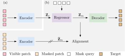
Figure 1: The pipeline of context autoencoder. Our approach (a) feeds visible patches into the encoder and extracts their representations $\mathbf{Z}_{v}$ and then (b) completes the pretext tasks: predict the representations $\mathbf{Z}_{m}$ of the masked patches from the visible patches in the encoded representation space through latent contextual regressor and prediction alignment, and reconstruct the masked patches from the predicted representations $\mathbf{Z}_{m}$ of masked patches. The pretrained encoder in (a) is applied to downstream tasks by simply replacing the pretext task part (b) with the downstream task part. $//$ means stop gradient.

The typical MIM methods, such as BEiT bao2021beit , the method studied in the ViT paper DosovitskiyB0WZ21 , and iBoT zhou2021ibot , use a single ViT architecture to solve the pretraining task i.e., reconstructing the patch tokens or the pixel colors. These methods mix the two tasks: learning the encoder (representation) and reconstructing the masked patch. The subsequent method, masked autoencoder (MAE) he2021masked adopts an encoder-decoder architecture, partially decoupling the two tasks. As a result, the representation quality is limited. Most previous methods, except iBoT zhou2021ibot , lack an explicit modeling between encoded representations of visible patches and masked patches.

We present a context autoencoder (CAE) approach, illustrated in Figure 1, for improving the encoding quality. We pretrain the encoder through making predictions for the masked patches in the encoded representation space. The pretraining task is a combination of masked representation prediction and masked patch reconstruction. the pretraining network is an encoder-regressor-decoder architecture. The encoder takes only the visible patches as input and learns the representations only for the visible patches. The regressor predicts the masked patch representations, which is expected to be aligned with the representations of the masked patches computed from the encoder, from the visible patch representations. The decoder reconstructs the masked patches from the predicted masked patch representations without receiving the representations of the visible patches.

The prediction in the encoded representation space from the visible patches to the masked patches generates a plausible semantic guess for the masked patches, which lies in the same semantic space for the visible patches. We assume that the prediction is easier if the encoded representations take higher semantics and that the accurate prediction encourages that the encoded representations take on a larger extent of semantics, empirically validated by the experiments.

The CAE design also encourages the separation of learning the encoder and completing the pretraining tasks: the responsibility of representation learning is mainly taken by the encoder and the encoder is only for representation learning. The reasons include: the encoder in the top stream in Figure 1 operates only on visible patches, only focusing on learning semantic representations; the regression is done on the encoded representation space, as a mapping between the representations of the visible patches and the masked patches; the decoder operates only on the predicted representations of the masked patches.

We present the empirical performance of our approach on downstream tasks, semantic segmentation, object detection and instance segmentation, and classification. The results show that our approach outperforms supervised pretraining, contrastive self-supervised pretraining, and other MIM methods.

2 Related Work

Self-supervised representation learning has been widely studied in computer vision , including: context prediction CarlDoersch2015UnsupervisedVR ; tian2021semantic , clustering-based methods xie2016unsupervised ; yang2016joint ; caron2018deep ; asano2019self ; zhuang2019local ; huang2019unsupervised ; caron2019unsupervised ; PriyaGoyal2021SelfsupervisedPO , contrastive self-supervised learning li2020prototypical ; AaronvandenOord2018RepresentationLW ; henaff2020data ; wang2022repre , instance discrimination dosovitskiy2014discriminative ; dosovitskiy2015discriminative , image discretization gidaris2020learning ; gidaris2020online , masked image modeling li2021mst ; fang2022corrupted ; tian2022beyond , and information maximization ermolov2021whitening ; zbontar2021barlow ; bardes2021vicreg . The following mainly reviews closely-related methods.

Autoencoding. Traditionally, autoencoders were used for dimensionality reduction or feature learning phdthesis_LeCun ; gallinari1987memoires ; hinton1994autoencoders ; hinton2006reducing ; ranzato2007efficient ; vincent2008extracting ; kingma2013auto . The denoising autoencoder (DAE) is an autoencoder that receives a corrupted data point as input and is trained to estimate the original, uncorrupted data point as its output. The variants or modifications of DAE were adopted for self-supervised representation learning, e.g., corruption by masking pixels VincentLLBM10 ; pathak2016context ; chen2020generative , removing color channels zhang2016colorful , shuffling image patches noroozi2016unsupervised , denoising pixel-level noise atito2021sit and so on.

Contrastive self-supervised learning. Contrastive self-supervised learning, referring in this paper to the self-supervised approaches comparing random views with contrastive loss or simply MSE loss that are related as shown in GarridoCBNL22 , has been popular for self-supervised representation learning ChenK0H20 ; He0WXG20 ; YonglongTian2020WhatMF ; ChenXH21 ; grill2020bootstrap ; CaronTMJMBJ21 ; chen2021exploring ; caron2020unsupervised_swav ; wu2018unsupervised ; XiangyuPeng2022CraftingBC . The basic idea is to maximize the similarity between the views augmented from the same image and optionally minimize the similarity between the views augmented from different images. Random cropping is an important augmentation scheme, and thus typical contrastive self-supervised learning methods (e.g., MoCo v3) tend to learn knowledge mainly from the central regions of the original images. Some dense variants wang2021dense ; xie2021propagate eliminate the tendency in a limited degree by considering an extra contrastive loss with dense patches.

Masked image modeling. Motivated by BERT for masked language modeling DevlinCLT19 , the method studied in DosovitskiyB0WZ21 and BEiT bao2021beit use the ViT structure to solve the masked image modeling task, e.g., estimate the pixels or the discrete tokens. The follow-up work, iBOT zhou2021ibot , combines the MIM method (BEiT) and a contrastive self-supervised approach (DINO CaronTMJMBJ21 ). But they do not have explicitly an encoder for representation learning or a decoder for pretraining task completion, and the ViT structure is essentially a mixture of encoder and decoder, limiting the representation learning quality.

Several subsequent MIM methods are developed to improve the encoder quality, such as designing pretraining architectures: Masked Autoencoder (MAE) he2021masked , SplitMask el2021large , and Simple MIM (SimMIM) xie2021simmim ; adopting new reconstruction targets: Masked Feature Prediction (MaskFeat) wei2021masked , Perceptual Codebook for BEiT (PeCo) dong2021peco , and data2vec BaevskiHXBGA22 . The technical report  of our approach was initially published as an arXiv paper CAE2022 , and was concurrent to data2vec BaevskiHXBGA22 , MAE he2021masked , and other methods, such as el2021large ; xie2021simmim . After that, MIM methods have developed rapidly, e.g., extended to frequency/semantic domain xie2022masked ; liu2022devil ; wei2022mvp ; li2022mc , combined with contrastive self-superivsed learning tao2022siamese ; jing2022masked ; yi2022masked ; huang2022contrastive , efficient pretraining zhang2022hivit ; huang2022green ; chen2022efficient , mask strategy design kakogeorgiou2022hide ; li2022semmae ; li2022uniform , scalability of MIM xie2022data , and interpretation of MIM xie2022revealing ; li2022architecture ; kong2022understanding .

The core idea of our approach is making predictions in the encoded representation space. We jointly solve two pretraining tasks: masked representation prediction - predict the representations for the masked patches, where the representations lie in the representation space output from the encoder, and masked patch reconstruction - reconstruct the masked patches.

Our approach is clearly different from MAE he2021masked (Figure 2 (top)). Our approach introduces an extra pretraining task, masked representation prediction, and encourages the separation of two roles: learning the encoder and completing pretraining tasks; in contrast, MAE partially mixes the two roles, and has no explicit prediction of masked patch representations.

On the other hand, our approach differs from data2vec BaevskiHXBGA22 and iBoT zhou2021ibot (Figure 2 (bottom)). Similar to BEiT, in data2vec and iBoT, there is no explicit module separation of learning the encoder and estimating the mask patch representations, and the target representations are formed from the full view (as the teacher) with the same network as the student network for processing the masked view and predicting the masked patch representations (except a centering process in iBoT for the teacher following DINO). In contrast, our approach is simple: form the target representations merely from the output of the encoder, and the encoder-regressor design is straightforward and explainable: the regressor predicts the representations of masked patches to match the representations computed directly from the encoder.

‘

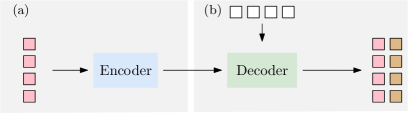
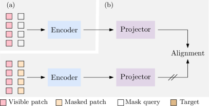
Figure 2: The pipeline of MAE (top), and the MIM part of iBoT (bottom). The centering module is not depicted in the bottom stream. The pretrained encoder in (a) is applied to downstream tasks by simply replacing the pretext task part (b) with the downstream task part. $//$ means stop gradient.

3 Approach

3.1 Architecture

Our context autoencoder (CAE) is a masked image modeling approach. The network shown in Figure 1 is an encoder-regressor-decoder architecture. The key is to make predictions from visible patches to masked patches in the encoded representation space. The pretraining tasks include: masked representation prediction and masked patch reconstruction.

We randomly split an image into two sets of patches: visible patches $\mathbf{X}_{v}$ and masked patches $\mathbf{X}_{m}$. The encoder takes the visible patches as input; the regressor predicts the representations of the masked patches, which are expected to be aligned with the representations computed from the encoder, from the representations of the visible patches conditioned on the positions of masked patches; the decoder reconstructs the masked patches from the predicted encoded representations.

Encoder. The encoder $\mathcal{F}$ maps the visible patches $\mathbf{X}_{v}$ to the latent representations $\mathbf{Z}_{v}$. It only handles the visible patches. We use the ViT to form our encoder. It first embeds the visible patches by linear projection as patch embeddings, and adds the positional embeddings $\mathbf{P}_{v}$. Then it sends the combined embeddings into a sequence of transformer blocks that are based on self-attention, generating $\mathbf{Z}_{v}$.

Regressor. The latent contextual regressor $\mathcal{H}$ predicts the latent representations $\mathbf{Z}_{m}$ for the masked patches from the latent representations $\mathbf{Z}_{v}$ of the visible patches output from the encoder conditioned on the positions of the masked patches. We form the latent contextual regressor $\mathcal{H}$ using a series of transformer blocks that are based on cross-attention.

The initial queries $\mathbf{Q}_{m}$, called mask queries, are mask tokens that are learned as model parameters and are the same for all the masked patches. The keys and the values are the same before linear projection and consist of the visible patch representations $\mathbf{Z}_{v}$ and the output of the previous cross-attention layer (mask queries for the first cross-attention layer). The corresponding positional embeddings of the masked patches are considered when computing the cross-attention weights between the queries and the keys. In this process, the latent representations $\mathbf{Z}_{v}$ of the visible patches are not updated.

Decoder. The decoder $\mathcal{G}$ maps the latent representations $\mathbf{Z}_{m}$ of the masked patches to some forms of masked patches, $\mathbf{Y}_{m}$. The decoder, similar to the encoder, is a stack of transformer blocks that are based on self-attention, followed by a linear layer predicting the targets. The decoder only receives the latent representations of the masked patches (the output of the latent contextual regressor), and the positional embeddings of the masked patches as input without directly using the information of the visible patches.

3.2 Objective Function

Masking. Following BEiT bao2021beit , we adopt the random block-wise masking strategy (illustrated in Figure 3) to split the input image into two sets of patches, visible and masked patches. For each image, $98$ of $196$ ($14\times 14$) patches are masked.

Targets. The targets $\bar{\mathbf{Z}}_{m}$ for the representations of the masked patches are formed as follows. We feed the masked patches $\mathbf{X}_{m}$ into the encoder, which is the same as the one for encoding visible patches, and generate the representations $\bar{\mathbf{Z}}_{m}$ of the masked patches as the representation targets.

The targets $\bar{\mathbf{Y}}_{m}$ for the patch reconstruction are formed by the discrete tokenizer, e.g., the tokenizer trained with d-VAE on ImageNet-$1$K without using the labels or the DALL-E tokenizer (trained with d-VAE on $400$M images) RameshPGGVRCS21 used in BEiT bao2021beit . The input image is fed into the tokenizer, assigning a discrete token to each patch for forming the reconstruction targets $\bar{\mathbf{Y}}_{m}$.

Loss function. The loss function consists of a reconstruction loss: $\ell_{y}(\mathbf{Y}_{m},\bar{\mathbf{Y}}_{m})$, and an alignment loss: $\ell_{z}(\mathbf{Z}_{m},\bar{\mathbf{Z}}_{m})$, corresponding to masked patch reconstruction and masked representation prediction, respectively. The whole loss is a weighted sum:

$$\quad\quad\quad\quad\quad\ell_{y}(\mathbf{Y}_{m},\bar{\mathbf{Y}}_{m})+\lambda~{}\ell_{z}(\mathbf{Z}_{m},\operatorname{sg}[\bar{\mathbf{Z}}_{m}]).$$ (1)

We use the MSE loss for $\ell_{z}(\mathbf{Z}_{m},\bar{\mathbf{Z}}_{m})$ and the cross-entropy loss for $\ell_{y}(\mathbf{Y}_{m},\bar{\mathbf{Y}}_{m})$. $\operatorname{sg}[\cdot]$ stands for stop gradient. $\lambda$ is $2$ in our experiments.

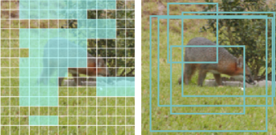
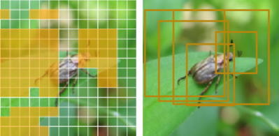
Figure 3: Illustration of random block-wise sampling ($1$st and $3$rd images) and random cropping ($2$nd and $4$th images). The colored regions are masked regions. The boxes correspond to cropped regions. Random block-wise sampling is used in our approach. Random cropping is a key data-augmentation scheme for contrastive self-supervised pretraining.

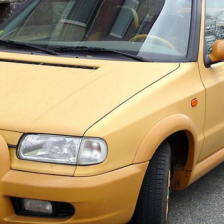
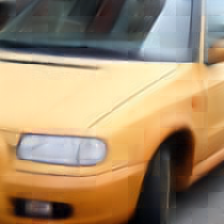
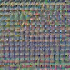
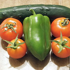
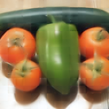
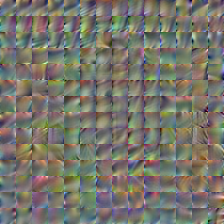
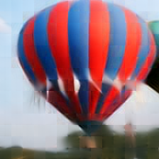
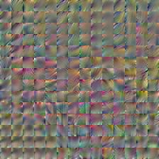
Figure 4: Illustrating that predictions are made in the representation space. We reconstruct the image by feeding the full image ($1$st, $4$th, and $7$th) into the pretrained CAE encoder and then the pretrained CAE decoder outputting the reconstructed image ($2$nd, $5$th, and $8$th). It can be seen that the image can be constructed with the semantics kept when skipping latent contextual regressor, verifying the input and the predicted representations lie in the same space. We also show the reconstructed images ($3$rd, $6$th, and $9$th) from the encoder and the decoder pretrained without the alignment constraint. We can see that those images are meaningless, indicating that the alignment constraint is critical for ensuring that predictions are made in the representation space.

4 Discussions

4.1 Analysis

Predictions are made in the encoded representation space. Our CAE attempts to make predictions in the encoded representation space: predict the representations for the masked patches from the encoded representations of the visible patches. In other words, it is expected that the output representations of the latent contextual regressor also lie in the encoded representation space, which is ensured by prediction alignment. This encourages the learned representation to take on a large extent of semantics for prediction from visible patches to masked patches, benefiting the representation learning of the encoder.

We empirically verify that the predicted representations lie in the encoded representation space through image reconstruction. We train the CAE using the pixel colors as the prediction targets, for two cases: with and without the alignment, i.e., masked representation prediction. For reconstruction, we feed all the patches (without masking, all the image patches are visible) of an image (from the ImageNet validation set) into the pretrained encoder, then skip the latent contextual regressor and directly send all the encoded patch representations to the pretrained decoder for reconstructing the whole image.

Figure 4 provides reconstruction results for several examples randomly sampled from the ImageNet-$1$K validation set. One can see that our approach can successfully reconstruct the images, implying that the input and output representations of latent contextual regressor are in the same space. In contrast, without the alignment, the reconstructed images are noisy, indicating the input and output representations of latent contextual regressor are in different spaces. The results suggest that the explicit prediction alignment is critical for ensuring that predictions are made in the encoded representation space.

Representation alignment in CAE and contrastive self-supervised learning. Representation alignment is also used in contrastive self-supervised learning methods, such as MoCo, BYOL, SimCLR, and methods mixing contrastive self-supervised learning and masked image modeling, such as iBOT, and MST. The alignment loss could be the MSE loss or the contrastive loss that CAE may also take advantage of.

In the CAE, the alignment is imposed over the representations $\mathbf{Z}_{m}=\mathcal{H}(\mathcal{F}(\mathbf{X}_{v}))$ - predicted from the representations $\mathcal{F}(\mathbf{X}_{v})$ of visible patches through the regressor $\mathcal{H}$, and the representations $\bar{\mathbf{Z}}_{m}=\mathcal{F}(\mathbf{X}_{m})$ - computed from the encoder $\mathcal{F}$. Both $\mathbf{Z}_{m}$ and $\bar{\mathbf{Z}}_{m}$ are about the masked patches, and lie in the representation space output from the encoder.

Differently, the alignment in the most contrastive self-supervised learning methods is imposed over the representations $\{\mathcal{P}(\mathcal{F}(\mathbf{V}_{1})),\mathcal{P}(\mathcal{F}(\mathbf{V}_{2})),\cdots,\mathcal{P}(\mathcal{F}((\mathbf{V}_{N}))\}$, where $\mathcal{P}$ is a projector, and some views may be processed with the EMA version of the encoder and the projector. The $N$ representations to be aligned are about different views $\{\mathbf{V}_{1},\mathbf{V}_{2},\cdots,\mathbf{V}_{N}\}$ (in iBoT and MST, the views are masked views and full views), and are not directly output from the encoder. It is not quite clear how the projector works, and it is reported in MIMPart2022 that the projector is a part-to-whole process mapping the object part representation to the whole object representation for contrastive self-supervised learning.

4.2 Connection

Relation to autoencoder. The original autoencoder phdthesis_LeCun ; gallinari1987memoires ; hinton1994autoencoders consists of an encoder and a decoder. The encoder maps the input into a latent representation, and the decoder reconstructs the input from the latent representation. The denoising autoencoder (DAE) VincentLLBM10 , a variant of autoencoder, corrupts the input by adding noises and still reconstructs the non-corrupted input.

Our CAE encoder is similar to the original autoencoder and also contains an encoder and a decoder. Different from the autoencoder where the encoder and the decoder process the whole image, our encoder takes a portion of patches as input and our decoder takes the estimated latent representations of the other portion of patches as input. Importantly, the CAE makes predictions in the latent space from the visible patches to the masked patches.

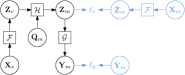
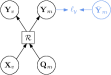
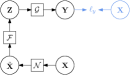
Figure 5: The computational graphs for (a) a context autoencoder (CAE), (b) BEiT bao2021beit , (c) a denoising autoencoder (DAE), and (d) MAE he2021masked and the one stream in SplitMask el2021large . The parts in cornflower blue are for loss function. (a) The encoder $\mathcal{F}$ receives visible patches $\mathbf{X}_{v}$ and outputs their latent representations $\mathbf{Z}_{v}$. The latent contextual regressor $\mathcal{H}$ predicts the latent representations $\mathbf{Z}_{m}$ for masked patches from $\mathbf{Z}_{v}$. The decoder predicts the targets $\mathbf{Y}_{m}$ for masked patches from $\mathbf{Z}_{m}$. $\ell_{z}$ and $\ell_{y}$ are the loss functions. During training, the gradient is stopped for $\bar{\mathbf{Z}}_{m}$. See the detail in Section 3. (b) The input includes both visible patches $\mathbf{X}_{v}$ and mask queries $\mathbf{Q}_{m}$ representing masked patches, and the representations for them are updated within the function $\mathcal{R}$. (c) The function $\mathcal{N}$ is a noising function generating the noisy version $\tilde{\mathbf{X}}$ from the input $\mathbf{X}$. $\mathcal{F}$ and $\mathcal{G}$ are the normal encoder and decoder, respectively. (d) The two functions, $\mathcal{F}^{\prime}$ and $\mathcal{R}$, are both based on self-attention. $\mathcal{F}^{\prime}$ (called encoder in MAE) only processes the visible patches $\mathbf{X}_{v}$, and $\mathcal{R}$ (called decoder in MAE) processes both the latent representations $\mathbf{Z}_{v}$ of the visible patches and the mask queries ($\mathbf{Q}_{m}$) and updates them simultaneously. For simplicity, the positional embeddings are not included in computational graphs. (a) CAE and (c) DAE perform the encoding and MIM task completion roles explicitly and separately, (b) BEiT and (d) MAE perform the encoding and MIM task completion roles implicitly and simultaneously.

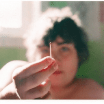
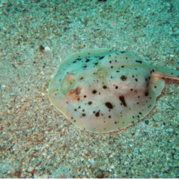
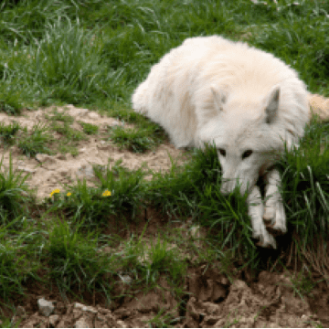
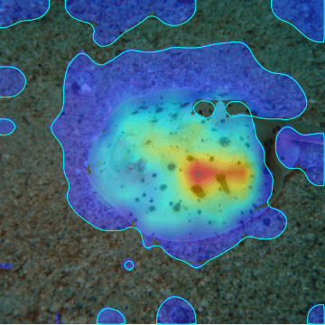
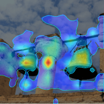
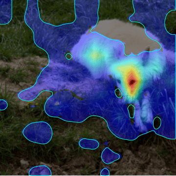
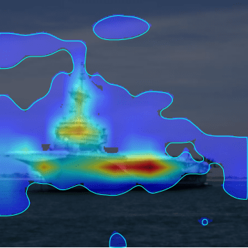
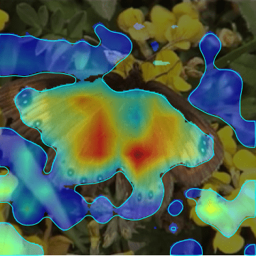
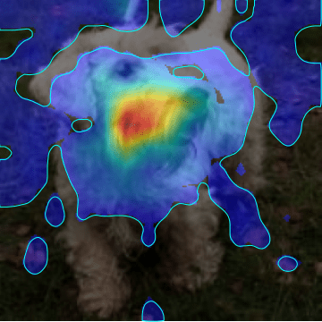
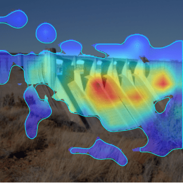
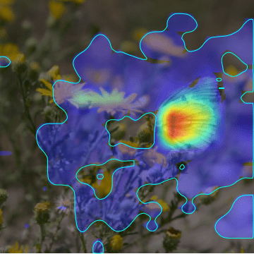
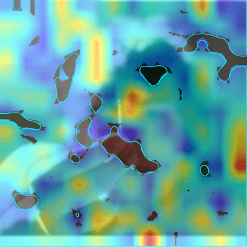
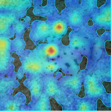
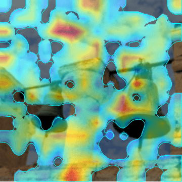
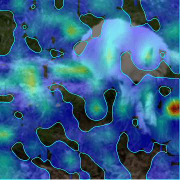
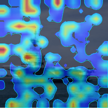
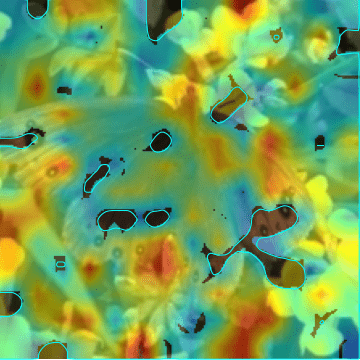
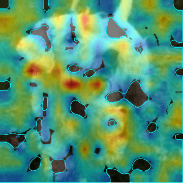
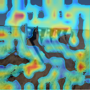
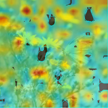
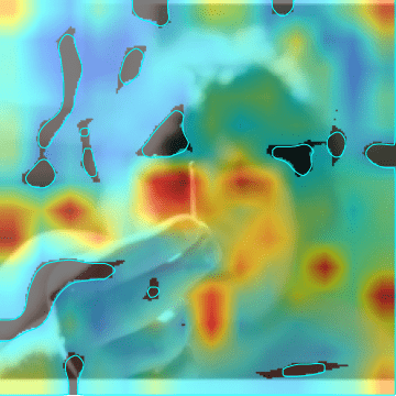
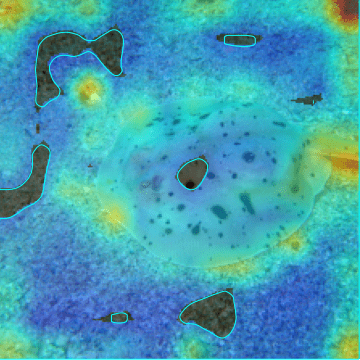
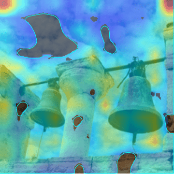
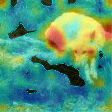
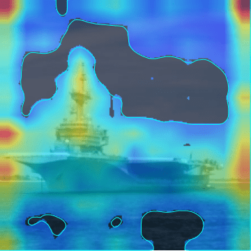
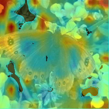
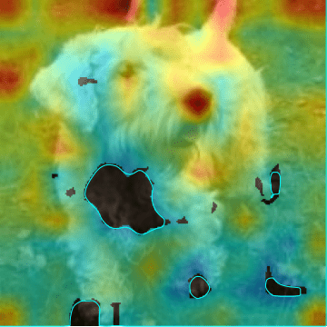
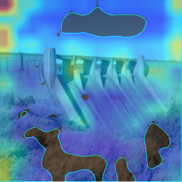
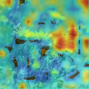
Figure 6: Illustrating the attention map averaged over $12$ attention heads between the class token and the patch tokens in the last layer of the ViT encoder pretrained on ImageNet-$1$K. The region inside the blue contour is obtained by thresholding the attention weights to keep $50\%$ of the mass. The four rows are: (1) input image, (2) MoCo v3, a typical contrastive self-supervised learning method, (3) MAE, and (4) our CAE. One can see that MoCo v3 tends to focus mainly on the centering regions and little on other patches, and our CAE tends to consider almost all the patches.

Relation to BEiT, iBoT and MAE. The CAE encoder processes the visible patches, to extract their representations, without making predictions for masked patches. Masked representation prediction is made through the regressor and the prediction alignment, ensuring that the output of the regressor lies in the representation space same with the encoder output. The decoder only processes the predicted representations of masked patches. Our approach encourages that the encoder takes the responsibility of and is only for representation learning.

In contrast, BEiT bao2021beit and the MIM part of iBOT do not separate the representation extraction role and the task completion role and uses a single network, with both the visible and masked patches as the input, simultaneously for the two roles. In MAE he2021masked , the so-called decoder may play a partial role for representation learning as the representations of the visible patches are also updated in the MAE decoder. Unlike CAE, MAE, iBoT, BEiT do not explicitly predict the representations of masked patches from the representations of visible patches (that lie in the encoded representation space) for masked patches.

When the pretrained encoder is applied to downstream tasks, one often replaces the pretext task completion part using the downstream task layer, e.g., segmentation layer or detection layer. The separation of representation learning (encoding) and pretext task completion helps that downstream task applications take good advantage of representation pretraining.

We provide the computational graph for CAE, BEiT bao2021beit , denoising autoencoder, Masked Autoencoder he2021masked and SplitMask el2021large (one stream) in Figure 5. Compared to our CAE, the main issue of MAE is that the so-called decoder $\mathcal{R}$ might have also the encoding role, i.e., learning semantic representations of the visible patches.

Comparison to contrastive self-supervised learning. Typical contrastive self-supervised learning methods, e.g., SimCLR ChenK0H20 and MoCo He0WXG20 ; ChenXH21 , pretrain the networks by solving the pretext task, maximizing the similarities between augmented views (e.g., random crops) from the same image and minimizing the similarities between augmented views from different images.

It is shown in ChenK0H20 that random cropping plays an important role in view augmentation for contrastive self-supervised learning. Through analyzing random crops (illustrated in Figure 3), we observe that the center pixels in the original image space have large chances to belong to random crops. We suspect that the global representation, learned by contrastive self-supervised learning for a random crop possibly with other augmentation schemes, tends to focus mainly on the center pixels in the original image, so that the representations of different crops from the same image can be possibly similar. Figure 6 (the second row) shows that the center region of the original image for the typical contrastive self-supervised learning approach, MoCo v3, is highly attended. The part in random crops corresponding to the center of the original image is still attended as shown in Figure 8.

In contrast, our CAE method (and other MIM methods) randomly samples the patches from the augmented views to form the visible and masked patches. All the patches are possible to be randomly masked for the augmented views and accordingly the original image. Thus, the CAE encoder needs to learn good representations for all the patches, to make good predictions for the masked patches from the visible patches. Figure 6 (the third row) illustrates that almost all the patches in the original images are considered in our CAE encoder.

Considering that the instances of the $1000$ categories in ImageNet-$1$K locate mainly around the center of the original images russakovsky2015imagenet , typical contrastive self-supervised learning methods, e.g., MoCo v3, learn the knowledge mainly about the $1000$ categories, which is similar to supervised pretraining. But our CAE and other MIM methods are able to learn more knowledge beyond the $1000$ categories from the non-center image regions. This indicates that the CAE has the potential to perform better for downstream tasks.

    

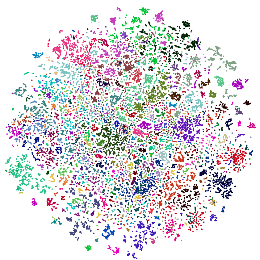
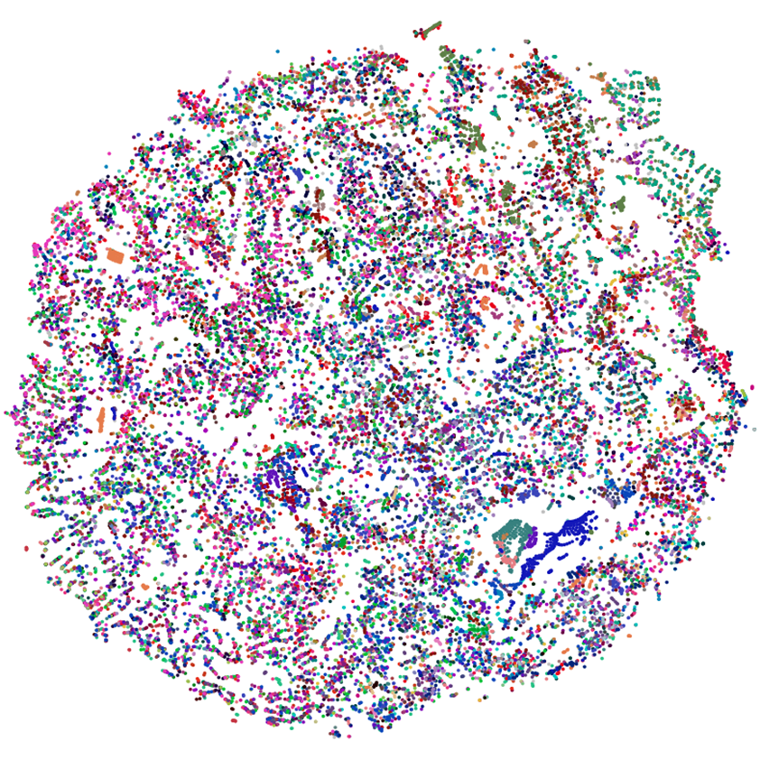
Figure 7: t-SNE visualization (one color for one category) of representations extracted from the images in ADE$20$K. Left: ViT pretrained with our CAE; Right: ViT with random weights.

4.3 Interpretation

Intuitive Interpretation for CAE. Humans are able to hallucinate what appears in the masked regions and how they appear according to the visible regions. We speculate that humans do this possibly in a way similar as the following example: given that only the region of the dog’s head is visible and the remaining parts are missing, one can (a) recognize the visible region to be about a dog, (b) predict the regions where the other parts of the dog appear, and (c) guess what the other parts look like.

Our CAE encoder is in some sense like the human recognition step (a). It understands the content by mapping the visual patches into latent representations that lie in the subspace that corresponds to the category dog. The latent contextual regressor is like step (b). It produces a plausible hypothesis for the masked patches, and describes the regions corresponding to the other parts of the dog using latent representations. The CAE decoder is like step (c), mapping the latent representations to the targets. It should be noted that the latent representations might contain other information besides the semantic information, e.g., the part information and the information for making predictions.

We adopt t-SNE van2008visualizing to visualize the high-dimensional patch representations output from our CAE encoder on ADE$20$K zhou2017scene in Figure 7. ADE$20$K has a total of $150$ categories. For each patch in the image, we set its label to be the category that more than half of the pixels belong to. We collect up to $1000$ patches for each category from sampled $500$ images. As shown in the figure, the latent representations of CAE are clustered to some degree for different categories (though not perfect as our CAE is pretrained on ImageNet-1K). Similar observations could be found for other MIM methods.

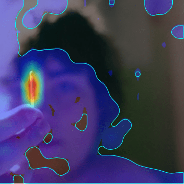
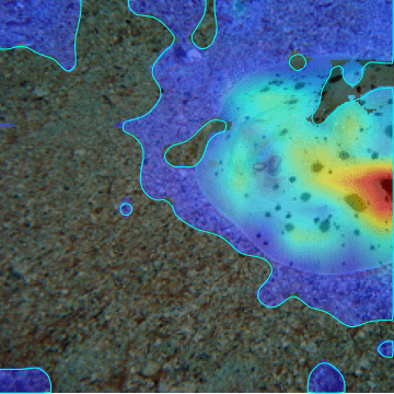
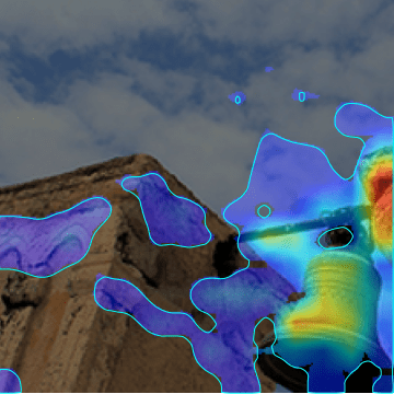
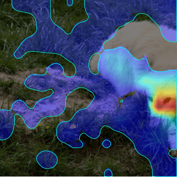
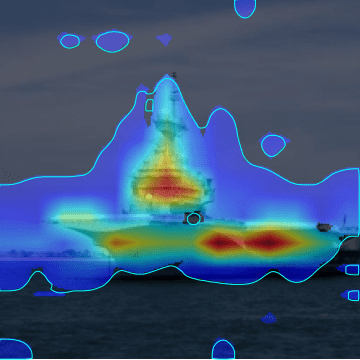
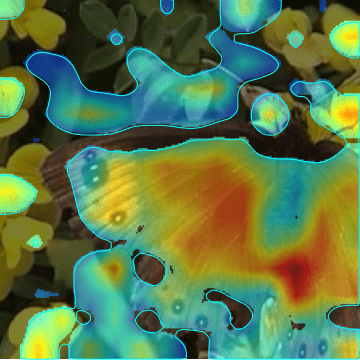
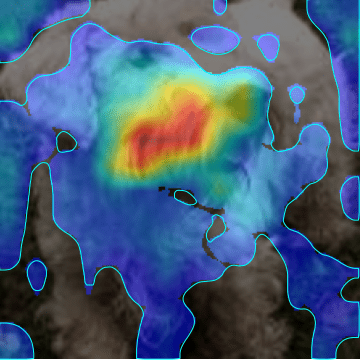
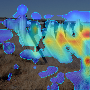
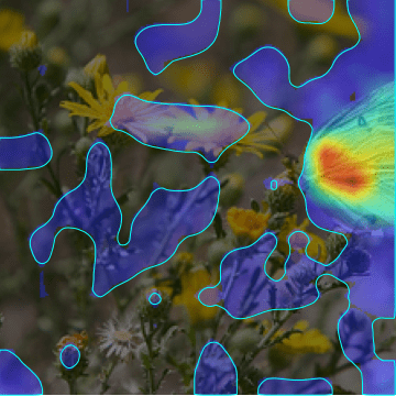
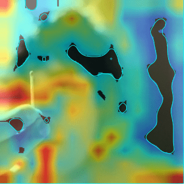
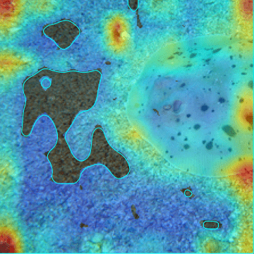
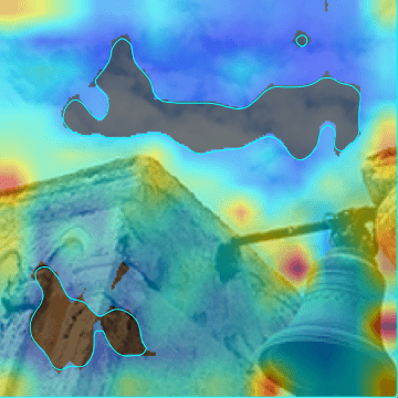
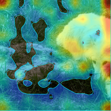
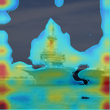
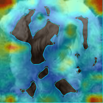
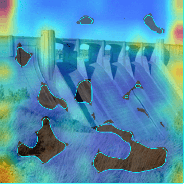
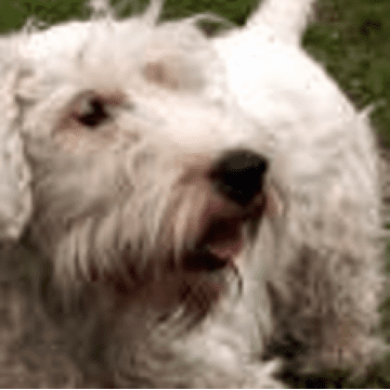
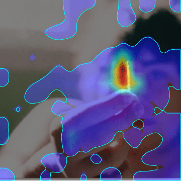
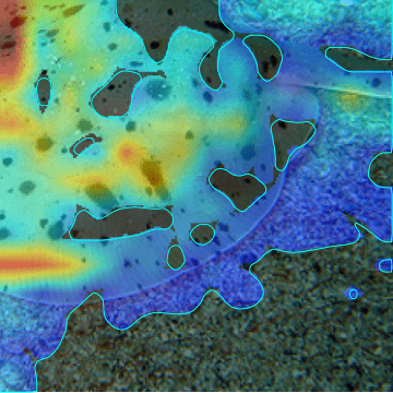
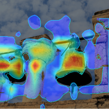
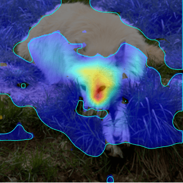
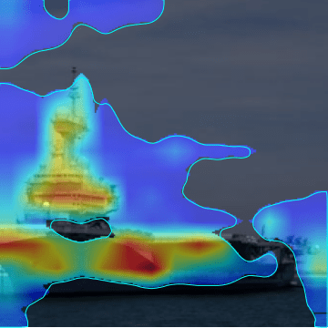
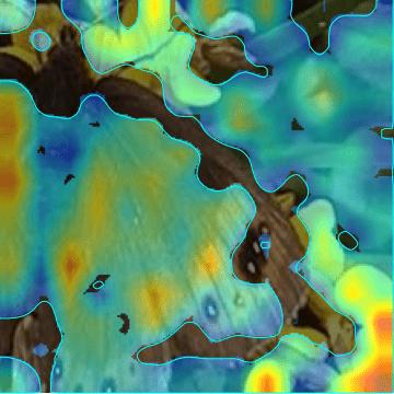
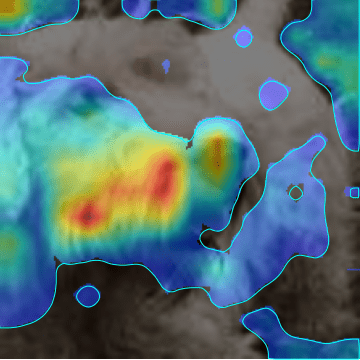
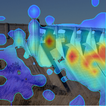
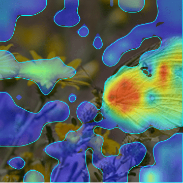
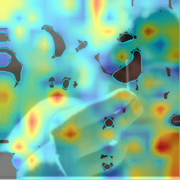
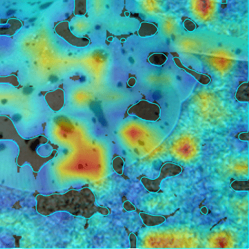
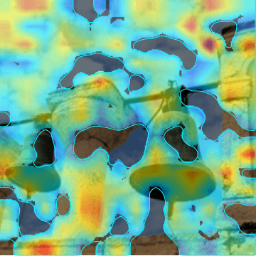
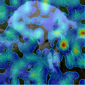
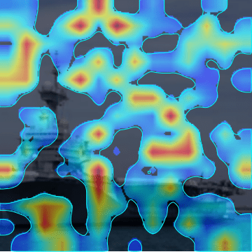
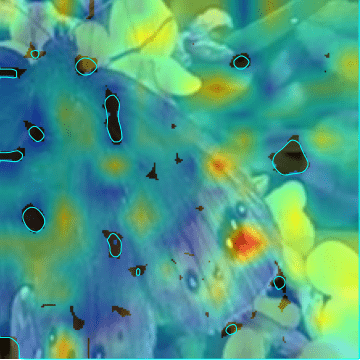
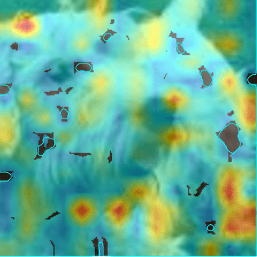
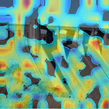
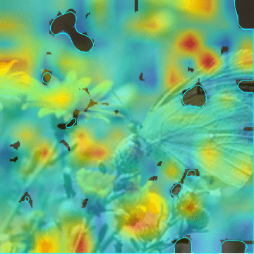
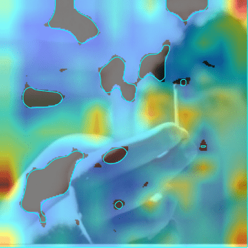
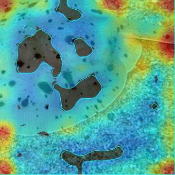
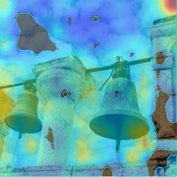
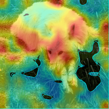
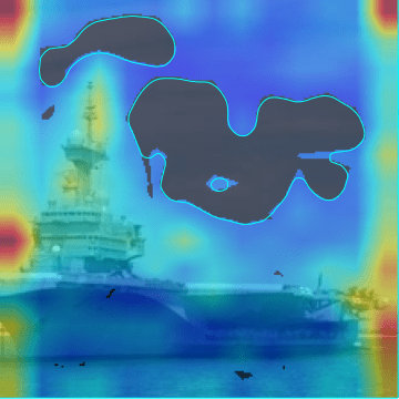
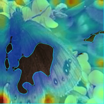
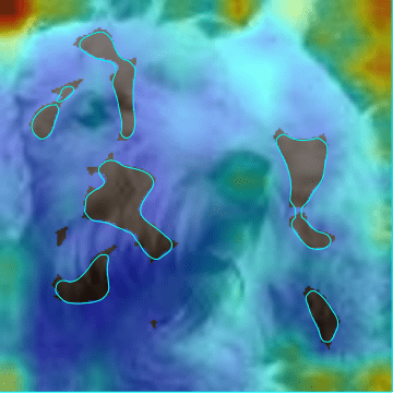
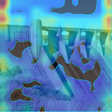
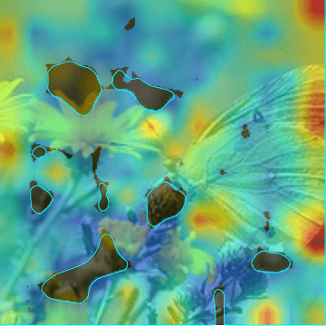
Figure 8: The attention maps over two sets of randomly cropped images (the $1$st the $5$th rows) for MoCo v3 (the $2$nd the $6$th rows), MAE (the $3$rd the $7$th rows), and our CAE (the $4$th the $8$th rows) pretrained on ImageNet-$1$K. The contrastive self-supervised learning method, MoCo v3, tends to focus mainly on the object region and little on other regions. In contrast, MIM-based models, CAE and MAE, tend to consider almost all the patches. The attention maps over the original images are shown in Figure 6.

Probabilistic interpretation for CAE. The MIM problem can be formulated in the probabilistic form, maximizing the probability of the predictions $\mathbf{Y}_{m}$ of the masked patches given the conditions, the visible patches $\mathbf{X}_{v}$, the positions $\mathbf{P}_{v}$ of the visible patches, and the positions $\mathbf{P}_{m}$ of the masked patches: $P(\mathbf{Y}_{m}\mid\mathbf{X}_{v},\mathbf{P}_{v},\mathbf{P}_{m})$. It can be solved by introducing latent representations $\mathbf{Z}_{m}$ and $\mathbf{Z}_{v}$, with the assumption that $\mathbf{Z}_{v}$ and $\mathbf{P}_{m}$ ($\mathbf{Y}_{m}$ and $\mathbf{P}_{v}$) are conditionally independent (the probabilistic graphical model is given in Figure 9):

$$p(\mathbf{Y}_{m}\mid\mathbf{X}_{v},\mathbf{P}_{v},\mathbf{P}_{m})$$ (2)

$$= p(\mathbf{Z}_{v}\mid\mathbf{X}_{v},\mathbf{P}_{v},\mathbf{P}_{m})p(\mathbf{Z}_{m}\mid\mathbf{Z}_{v},\mathbf{P}_{v},\mathbf{P}_{m})$$

$$p(\mathbf{Y}_{m}\mid\mathbf{Z}_{m},\mathbf{P}_{v},\mathbf{P}_{m})$$ (3)

$$= p(\mathbf{Z}_{v}\mid\mathbf{X}_{v},\mathbf{P}_{v})p(\mathbf{Z}_{m}\mid\mathbf{Z}_{v},\mathbf{P}_{v},\mathbf{P}_{m})p(\mathbf{Y}_{m}\mid\mathbf{Z}_{m},\mathbf{P}_{m}).$$ (4)

Here, the equation from (2) to (3) is obtained from the probabilistic graphical model of CAE shown in Figure 9, and the removal of the condition $\mathbf{P}_{m}$ (from $p(\mathbf{Z}_{v}\mid\mathbf{X}_{v},\mathbf{P}_{v},\mathbf{P}_{m})$ to $p(\mathbf{Z}_{v}\mid\mathbf{X}_{v},\mathbf{P}_{v})$), and the condition $\mathbf{P}_{v}$ (from $p(\mathbf{Y}_{m}\mid\mathbf{Z}_{m},\mathbf{P}_{v},\mathbf{P}_{m})$ to $p(\mathbf{Y}_{m}\mid\mathbf{Z}_{m},\mathbf{P}_{m})$) from (3) to (4) is based on the conditional independence assumption. The three terms in (4) correspond to three parts of our CAE: the encoder, the latent contextual regressor, and the decoder, respectively.

Figure 9: The probabilistic graphical model of CAE. The other conditions of $\mathbf{Z}_{v}$, $\mathbf{Z}_{m}$, and $\mathbf{Y}_{m}$, the positions $\mathbf{P}_{v}$ and $\mathbf{P}_{m}$ of the visible and masked patches, are not plotted for simplicity.

Similarly, the latent representation alignment constraint can be written as a conditional probability, $P(\mathbf{Z}_{m}\mid\bar{\mathbf{Z}}_{m})$, where $\bar{\mathbf{Z}}_{m}$ is the masked patch representations computed from the encoder.

Intuitive interpretation for the contrastive self-supervised learning. We consider the case in ImageNet-$1$K that the object mainly lies in the center of an image. There are $N$ randomly sampled crops from an image, and each crop $\mathbf{I}_{n}$ contains a part of the center object, $\mathbf{O}_{n}$. To maximize the similarity between two crops $\mathbf{I}_{m}$ and $\mathbf{I}_{n}$, the pretraining might contain the processes: select the regions $\mathbf{O}_{m}$ and $\mathbf{O}_{n}$ from the two crops $\mathbf{I}_{m}$ and $\mathbf{I}_{n}$, extract their features $\mathbf{f}_{om}$ and $\mathbf{f}_{on}$, and predict the feature of the object, $\mathbf{f}_{o}$, from the part features $\mathbf{f}_{om}$ and $\mathbf{f}_{on}$. In this way, the features of the crops from the same image could be similar. Among the $N$ random crops, most crops contain a part of the object in the center, and a few crops that do not contain a part of the center object could be viewed as noises when optimizing the contrastive loss.

After pretrained on ImageNet-$1$K (where the object mainly lies in the center) the encoder is able to learn the knowledge of the $1000$ classes and localize the region containing the object belonging to the $1000$ classes. It is not necessary that the object lies in the center for the testing image, which is verified in Figure 8. This further verifies that MoCo v3 (contrastive self-supervised pretraining) pretrained on ImageNet-$1$K tends to attend to the object region, corresponding to the center region of the original image as shown in Figure 6.

5 Experiments

5.1 Implementation

We study the standard ViT small, base and large architectures, ViT-S ($12$ transformer blocks with dimension $384$), ViT-B ($12$ transformer blocks with dimension $768$) and ViT-L ($24$ transformer blocks with dimension $1024$). The latent contextual regressor consists of $4$ transformer blocks based on cross-attention in which self-attention over masked tokens and encoded visible patch representations is a choice but with slightly higher computation cost and a little lower performance, and the decoder consists of $4$ transformer blocks based on self-attention, and an extra linear projection for making predictions.

5.2 Training Details

Pretraining. The pretraining settings are almost the same as BEiT bao2021beit . We train the CAE on ImageNet-$1$K. We partition the image of $224\times 224$ into $14\times 14$ patches with the patch size being $16\times 16$. We use standard random cropping and horizontal flipping for data augmentation. We use AdamW loshchilov2017adamw for optimization and train the CAE for $300$/$800$/$1600$ epochs with the batch size being $2048$. We set the learning rate as $1.5$e-$3$ with cosine learning rate decay. The weight decay is set as $0.05$. The warmup epochs for $300$/$800$/$1600$ epochs pre-training are $10$/$20$/$40$, respectively. We employ drop path huang2016stochastic_depth rate $0.1$ and dropout rate $0$.

Linear probing. We use the LARS you2017large optimizer with momentum $0.9$. The model is trained for $90$ epochs. The batch size is $16384$, the warmup epoch is $10$ and the learning rate is $6.4$. Following  he2021masked , we adopt an extra BatchNorm layer SergeyIoffe2015BatchNA without affine transformation (affine=False) before the linear classifier. We do not use mixup HongyiZhang2017mixupBE , cutmix SangdooYun2019CutMixRS , drop path huang2016stochastic_depth , or color jittering, and we set weight decay as zero.

Attentive probing. The parameters of the encoder are fixed during attentive probing. A cross-attention module, a BatchNorm layer (affine=False), and a linear classifier are appended after the encoder. The extra class token representation in cross-attention is learned as model parameters. The keys and the values are the patch representations output from the encoder. There is no MLP or skip connection operation in the extra cross-attention module. We use the SGD optimizer with momentum $0.9$ and train the model for $90$ epochs. The batch size is $8192$, the warmup epoch is $10$ and the learning rate is $0.4$. Same as linear probing, we do not use mixup HongyiZhang2017mixupBE , cutmix SangdooYun2019CutMixRS , drop path, or color jittering, and we set weight decay as zero.

Fine-tuning on ImageNet. We follow the fine-tuning protocol in BEiT to use layer-wise learning rate decay, weight decay and AdamW. The batch size is $4096$, the warmup epoch is $5$ and the weight decay is $0.05$. For ViT-S, we train $200$ epochs with learning rate $1.6$e-$2$ and layer-wise decay rate $0.75$. For ViT-B, we train $100$ epochs with learning rate $8$e-$3$ and layer-wise decay rate $0.65$. For ViT-L, we train $50$ epochs with learning rate $2$e-$3$ and layer-wise decay rate $0.75$.

Semantic segmentation on ADE$20$K. We use AdamW as the optimizer. The input resolution is $512\times 512$. The batch size is $16$. For the ViT-B, the layer-wise decay rate is $0.65$ and the drop path rate is $0.1$. We search from four learning rates, $1$e-$4$, $2$e-$4$, $3$e-$4$ and $4$e-$4$, for all the results in Table 2. For the ViT-L, the layer-wise decay rate is $0.95$ and the drop path rate is $0.15$. We search from three learning rates for all the methods, $3$e-$5$, $4$e-$5$, and $5$e-$5$, We conduct fine-tuning for $160$K steps. We do not use multi-scale testing.

Object detection and instance segmentation on COCO. We utilize multi-scale training and resize the image with the size of the short side between $480$ and $800$ and the long side no larger than $1333$. The batch size is $32$. For the ViT-S, the learning rate is $3$e-$4$, the layer-wise decay rate is $0.75$, and the drop path rate is $0.1$. For the ViT-B, the learning rate is $3$e-$4$, the layer-wise decay rate is $0.75$, and the drop path rate is $0.2$. For the ViT-L, the learning rate is $2$e-$4$, the layer-wise decay rate is $0.8$, and the drop path rate is $0.2$. We train the network with the $1\times$ schedule: $12$ epochs with the learning rate decayed by $10\times$ at epochs $9$ and $11$. We do not use multi-scale testing. The Mask R-CNN implementation follows MMDetection mmdetection .

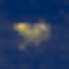
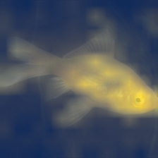
Figure 10: Illustrating the cross-attention unit in attentive probing. The attention map (bottom) is the average of cross-attention maps over $12$ heads between the extra class token and the patches. One can see that the attended region lies mainly in the object, which helps image classification.

5.3 Pretraining Evaluation

Linear probing. Linear probing is widely used as a proxy of pretraining quality evaluation for self-supervised representation learning. It learns a linear classifier over the image-level representation output from the pretrained encoder by using the labels of the images, and then tests the performance on the validation set.

Attentive probing. The output of the encoder pretrained with MIM methods are representations for all the patches. It is not suitable to linearly probe the representation, averagely-pooled from patch representations, because the image label in ImageNet-$1$K only corresponds to a portion of patches. It is also not suitable to use the default class token within the encoder because the default class token serves as a role of aggregating the patch representations for better patch representation extraction and is not merely for the portion of patches corresponding to the image label.

To use the image-level label as a proxy of evaluating the pretraining quality for the encoder pretrained with MIM methods, we need to attend the patches that are related to the label. We introduce a simple modification by using a cross-attention unit with an extra class token (that is different from the class token in the encoder) as the query and the output patch representations of the encoder as the keys and the values, followed by a linear classifier. The introduced cross-attention unit is able to care mainly about the patches belonging to the $1000$ classes in ImageNet-$1$K and remove the interference of other patches. Figure 10 illustrates the effect of the cross-attention unit, showing that the extra cross-attention unit can to some degree attend the regions that are related to the $1000$ ImageNet-$1$K classes.

Table 1: Pretraining quality evaluation in terms of fine-tuning (FT), linear probing (LIN), and attentive probing (ATT). ^‡ means the number of effective epochs in zhou2021ibot as they adopt multi-crop augmentation (equivalently take a larger number of epochs compared to one-crop augmentation). We report the top-$1$ accuracy (in the column ATT) of the supervised training approach DeiT touvron2020deit to show how far the ATT score is from supervised training. The scores for other models and our models are based on our implementations if not specified. Except that * denotes using the DALL-E tokenizer, CAE adopts the d-VAE tokenizer trained on ImageNet-1K only.

Method	#Epochs	#Crops	FT	LIN	ATT
Methods using ViT-S:
DeiT	$300$	-	-	-	$79.9$
MoCo v3	$\ \,600^{\ddagger}$	$2$	$81.7$	$73.1$	$73.8$
BEiT	$300$	$1$	$81.7$	$15.7$	$23.6$
CAE*	$300$	$1$	$\mathbf{82.0}$	$51.8$	$65.0$
Methods using ViT-B:
DeiT	$300$	-	-	-	$81.8$
MoCo v3	$\ \,600^{\ddagger}$	$2$	$83.0$	$76.2$	$77.0$
DINO	$\ \,1600^{\ddagger}$	$12$	$83.3$	$77.3$	$77.8$
BEiT	$300$	$1$	$83.0$	$37.6$	$49.4$
MAE	$300$	$1$	$82.9$	$61.5$	$71.1$
MAE	$1600$	$1$	$83.6$	$67.8$	$74.2$
SimMIM	$800$	$1$	$83.8$	$56.7$	-
iBOT	$\ \,1600^{\ddagger}$	$12$	$83.8$	$79.5$	$79.8$
CAE*	$300$	$1$	$83.6$	$64.1$	$73.8$
CAE*	$800$	$1$	$83.8$	$68.6$	$75.9$
CAE*	$1600$	$1$	$\mathbf{83.9}$	$70.4$	$77.1$
CAE	$1600$	$1$	$\mathbf{83.9}$	$71.4$	$77.4$
Methods using ViT-L:
MoCo v3†	$\ \,600^{\ddagger}$	$2$	$84.1$	-	-
BEiT†	$1600$	$1$	$85.2$	-	-
MAE	$1600$	$1$	$86.0$	$76.0$	$78.8$
CAE*	$1600$	$1$	$\mathbf{86.3}$	$78.1$	$81.2$
CAE	$1600$	$1$	$\mathbf{86.3}$	$77.9$	$81.2$

Results. Table 1 shows the results with three schemes, linear probing (LIN), attentive probing (ATT), and fine-tuning (FT) for representative contrastive self-supervised pretraining (MoCo v3 and DINO) and MIM (BEiT and MAE) methods, as well as our approach with the targets formed with the DALL-E tokenizer (trained on $400$M images) and the d-VAE tokenizer (trained on ImageNet-$1$K without using the labels), denoted as CAE* and CAE, respectively. The models of MAE with $300$ epochs and BEiT are pretrained by us using the official implementations, and other models are officially released models.

We highlight a few observations. The fine-tuning performance for these methods are very similar and there is only a minor difference similar to the observation zhou2021ibot . We think that the reason is that self-supervised pretraining and fine-tuning are conducted on the same dataset and no extra knowledge is introduced for image classification. The minor difference might come from the optimization aspect: different initialization (provided by pretrained models) for fine-tuning.

In terms of linear probing, the scores of the contrastive self-supervised learning methods, MoCo v3 and DINO, are higher than the MIM methods. This is as expected because contrastive self-supervised learning focuses mainly on learning the representations for $1000$ classes (See discussion in Section 4). The pretraining is relatively easier than existing MIM methods as contrastive self-supervised learning mainly cares about the $1000$ classes and MIM methods may care about the classes beyond the $1000$ classes.

For the MIM methods, the scores of attentive probing are much larger than linear probing. This validates our analysis: the MIM methods extract the representations for all the patches, and the classification task needs to attend the corresponding portion of patches.

The LIN and ATT scores are similar for contrastive self-supervised pretraining on ViT-B, e.g., $(76.2~{}\text{vs}~{}77.0)$ for MoCo v3 and $(77.3~{}\text{vs}~{}77.8)$ for DINO. This means that the extra cross-attention in attentive probing does not make a big difference, which is one more evidence for our analysis in Section 4 that they already focus mainly on the region where the instance in the $1000$ categories lies.

5.4 Downstream Tasks

Table 2: Semantic segmentation on ADE$20$K. All the results are based on the same implementation for semantic segmentation. #Epochs refers to the number of pretraining epochs. ^‡ means the number of effective epochs in zhou2021ibot as the method uses multi-crop pretraining augmentation (See Table 1). SplitMask el2021large is pretrained on ADE20K for 21000 epochs. ^†: these results are from he2021masked .

Method	#Epochs	mIoU
Methods using ViT-B:
SplitMask	–	$45.7$
BEiT	$300$	$45.5$
BEiT	$800$	$46.5$
mc-BEiT	800	$47.0$
DeiT	$300$	$47.0$
MoCo v3	$\ \,600^{\ddagger}$	$47.2$
DINO	$\ \,1600^{\ddagger}$	$47.2$
MAE	$300$	$45.8$
MAE	$1600$	$48.1$
Ge2-AE	$800$	$48.9$
A2MIM	$800$	$49.0$
iBOT	$\ \,1600^{\ddagger}$	$50.0$
CAE*	$300$	${48.3}$
CAE*	$800$	$49.7$
CAE*	$1600$	$\mathbf{50.2}$
CAE	$1600$	$50.1$
Methods using ViT-L:
MoCo v3†	$\ \,600^{\ddagger}$	$49.1$
BEiT†	$1600$	$53.3$
MAE	$1600$	$53.6$
CAE*	$1600$	$\mathbf{54.7}$
CAE	$1600$	$54.6$

Table 3: Object detection and instance segmentation on COCO. Mask R-CNN is adopted and trained with the $1\times$ schedule. All the results are based on the same implementation for object detection and instance segmentation. #Epochs refers to the number of pretraining epochs on ImageNet-$1$K. ^‡ means the number of effective epochs in zhou2021ibot (See Table 1).

Method	#Epochs	Supervised	Self-supervised	Object detection			Instance segmentation
				$\text{AP}^{b}$	$\text{AP}^{b}_{50}$	$\text{AP}^{b}_{75}$	$\text{AP}^{m}$	$\text{AP}^{m}_{50}$	$\text{AP}^{m}_{75}$
Methods using ViT-S:
DeiT	$300$	$\surd$	$\times$	$43.1$	$65.2$	$46.6$	$38.4$	$61.8$	$40.6$
MoCo v3	$\ \,600^{\ddagger}$	$\times$	$\surd$	$43.3$	$64.9$	$46.8$	$38.8$	$61.6$	$41.1$
BEiT	$300$	$\times$	$\surd$	$35.6$	$56.7$	$38.3$	$32.6$	$53.3$	$34.2$
CAE*	$300$	$\times$	$\surd$	$\mathbf{44.1}$	$64.6$	$48.2$	$\mathbf{39.2}$	$61.4$	$42.2$
Methods using ViT-B:
DeiT	$300$	$\surd$	$\times$	$46.9$	$68.9$	$51.0$	$41.5$	$65.5$	$44.4$
MoCo v3	$\ \,600^{\ddagger}$	$\times$	$\surd$	$45.5$	$67.1$	$49.4$	$40.5$	$63.7$	$43.4$
DINO	$\ \,1600^{\ddagger}$	$\times$	$\surd$	$46.8$	$68.6$	$50.9$	$41.5$	$65.3$	$44.5$
BEiT	$300$	$\times$	$\surd$	$39.5$	$60.6$	$43.0$	$35.9$	$57.7$	$38.5$
BEiT	$800$	$\times$	$\surd$	$42.1$	$63.3$	$46.0$	$37.8$	$60.1$	$40.6$
MAE	$300$	$\times$	$\surd$	$45.4$	$66.4$	$49.6$	$40.6$	$63.4$	$43.7$
MAE	$1600$	$\times$	$\surd$	$48.4$	$69.4$	$53.1$	$42.6$	$66.1$	$45.9$
iBOT	$\ \,1600^{\ddagger}$	$\times$	$\surd$	$48.2$	$69.7$	$52.8$	$42.7$	$66.5$	$46.0$
CAE*	$300$	$\times$	$\surd$	$48.4$	$69.2$	$52.9$	$42.6$	$66.1$	$45.8$
CAE*	$800$	$\times$	$\surd$	$49.8$	$70.7$	$54.6$	$43.9$	$67.8$	$47.4$
CAE*	$1600$	$\times$	$\surd$	$50.0$	$70.9$	$54.8$	$44.0$	$67.9$	$47.6$
CAE	$1600$	$\times$	$\surd$	$\mathbf{50.2}$	$71.0$	$54.9$	$\mathbf{44.2}$	$68.3$	$47.9$
Methods using ViT-L:
MAE	$1600$	$\times$	$\surd$	$54.0$	$74.3$	$59.5$	$47.1$	$71.5$	$51.0$
CAE*	$1600$	$\times$	$\surd$	$54.5$	$75.2$	$60.1$	$47.6$	$72.2$	$51.9$
CAE	$1600$	$\times$	$\surd$	$\mathbf{54.6}$	$75.2$	$59.9$	$\mathbf{47.6}$	$72.0$	$51.9$

Semantic segmentation on ADE$\mathbf{20}$K zhou2017scene . We follow the implementation bao2021beit to use UperNet xiao2018unified . The CAE with the tokenizers learned over ImageNet-$1$K performs almost the same as the tokenizers learned over $400$M images provided by DALL-E (CAE*), implying that the tokenizer trained on ImageNet-$1$K (without using the labels) or a larger dataset does not affect the pretraining quality and accordingly the downstream task performance.

Table 2 shows that using the ViT-B, our CAE* with $300$ training epochs performs better than DeiT, MoCo v3, DINO, MAE ($1600$ epochs) and BEiT. Our CAE* ($1600$ epochs) further improves the segmentation scores and outperforms MAE ($1600$ epochs), MoCo v3 and DeiT by $2.1$, $3.0$ and $3.2$, respectively. Using ViT-L, our CAE* ($1600$ epochs) outperforms BEiT ($1600$ epochs) and MAE ($1600$ epochs) by $1.4$ and $1.1$, respectively.

The superior results over supervised and contrastive self-supervised pretraining methods, DeiT, MoCo v3 and DINO, stem from that our approach captures the knowledge beyond the $1000$ classes in ImageNet-$1$K. The superior results over BEiT and MAE stems from that our CAE makes predictions in the encoded representation space and that representation learning and pretext task completion are separated.

Table 4: Top-1 classification accuracy on the Food-$101$, Clipart and Sketch datasets. The backbone is ViT-B.

Method	Supervised	Self-supervised	Food-$101$	Clipart	Sketch
Random Init.	$\times$	$\times$	82.77	$52.90$	$46.42$
DeiT	$\surd$	$\times$	$91.81$	$81.18$	$73.45$
DINO	$\times$	$\surd$	$91.67$	$80.72$	$73.13$
MAE	$\times$	$\surd$	$93.19$	$80.63$	$73.87$
CAE*	$\times$	$\surd$	$\mathbf{93.32}$	$\mathbf{81.84}$	$\mathbf{74.65}$

Table 5: Ablation studies for the decoder and the alignment constraint in our CAE. All the models are pretrained on ImageNet-$1$K with $300$ epochs.

Decoder	Alignment	LIN	ATT	FT	ADE Seg.	COCO Det.	#Params	Training Time
$\times$	$\times$	$60.3$	$71.2$	$82.9$	$47.0$	$46.9$	$120.32$ M	$1\times$
$\surd$	$\times$	$63.1$	$72.7$	$83.4$	$47.1$	$47.2$	$148.68$ M	$1.14\times$
$\times$	$\surd$	$62.0$	$71.5$	$83.4$	$47.1$	$47.2$	$120.32$ M	$1.12\times$
$\surd$	$\surd$	$64.1$	$73.8$	$83.6$	$48.3$	$48.4$	$148.68$ M	$1.24\times$

Table 6: The results of object detection and instance segmentation on COCO with the Cascaded Mask-RCNN framework ($1\times$ schedule). ViT-B is used for all experiments. All the detection results are from our implementation.

Method	#Epochs	$\text{AP}^{b}$	$\text{AP}^{m}$
MAE he2021masked	$1600$	$51.3$	$44.3$
mc-BEiT zhou2021ibot	$800$	$50.1$	$43.1$
iBOT zhou2021ibot	$1600$	$51.2$	$44.2$
CAE*	$300$	$51.6$	$44.6$
CAE*	$800$	$52.8$	$45.5$
CAE*	$1600$	$\mathbf{52.9}$	$\mathbf{45.5}$

Object detection and instance segmentation on COCO lin2014microsoft . We adopt the Mask R-CNN approach he2017mask that produces bounding boxes and instance masks simultaneously, with the ViT as the backbone. The results are given in Table 3. We report the box AP for object detection and the mask AP for instance segmentation. The observations are consistent with those for semantic segmentation in Table 2. Our CAE* ($300$ epochs, ViT-B) is superior to all the other models except that a little lower than MAE ($1600$ epochs). Our approach ($1600$ epochs) outperforms MAE ($1600$ epochs), MoCo v3 and DeiT by $1.6$, $4.5$ and $3.1$, respectively. Using ViT-L, our CAE achieves $54.6$ box AP and outperforms MAE by $0.6$.

We also report the results of object detection and instance segmentation on COCO with the Cascaded Mask R-CNN framework ZhaoweiCai2021CascadeRH in Table 6. Results show that our CAE performs better than other methods.

In addition, we conduct experiments on the scaling ability of CAE on the detection task. The detection model is built upon ViT-Huge DosovitskiyB0WZ21 , DINO HaoZhang2023DINODW , and Group DETR QiangChen2022GroupDF (see groupdetrv2 for more details). The ViT-Huge is pretrained on ImageNet-$22$K deng2009imagenet using CAE. We are the first to obtain $64.6$ mAP on COCO test-dev, which outperforms previous methods with larger models and more training data (e.g., BEIT-3 WenhuiWang2023ImageAA ($63.7$ mAP) and SwinV2-G ZeLiu2021SwinTV ($63.1$ mAP)).

Table 7: The effect of mask ratios. The backbone is ViT-B. Models are trained for $300$ epochs.

Mask Ratio	LIN	ATT	ADE Seg
$40\%$	$63.1$	$73.0$	$47.2$
$50\%$	$64.1$	$73.8$	$48.3$
$60\%$	$64.8$	$74.2$	$48.1$

Classification. We conduct fine-tuning experiments on three datasets: Food-$101$ bossard14 , Clipart castrejon2016learning , and Sketch castrejon2016learning . Results in Table 4 show that the proposed method outperforms the previous supervised method (DeiT) and self-supervised methods (DINO, MAE).

5.5 Ablation Studies

Decoder and alignment. The CAE architecture contains several components for pretraining the encoder: regressor and alignment for masked representation prediction, decoder with a linear layer for masked patch reconstruction. We observe that if the pretraining task, masked patch reconstruction, is not included, the training collapses, leading to a trivial solution. We thus study the effect of the decoder (when the decoder is removed, we use a linear layer to predict the targets), which is helpful for target reconstruction, and the alignment, which is helpful for representation prediction.

Table 5 shows the ablation results. We report the scores for linear probing, attentive probing, fine-tuning and downstream tasks: semantic segmentation on the ADE$20$K dataset and object detection on COCO with the DALL-E tokenizer as the target. One can see that the downstream task performance is almost the same when only the decoder is added and that the performance increases when the decoder and the alignment are both added. This also verifies that the alignment is important for ensuring that the predicted representations of masked patches lie in the encoded representation space and thus the predictions are made in the encoded representation space, and accordingly improving the representation quality. Without the decoder, the performance drops. This is because the reconstruction from the semantic representation to the low-level targets cannot be done through a single linear layer, and no decoder will deteriorate the semantic quality of the encoder. The additional computational cost, i.e. the number of parameters and training time, brought by the decoder and alignment is relatively small, e.g., increasing the number of parameters to $1.23\times$ and training time to $1.24\times$.

Mask ratio. We also conduct experiments with different mask ratios including $40\%$, $50\%$, and $60\%$. Results are listed in Table 7. We find that ratio $50\%$ gets better results than ratio $40\%$. Adopting a higher mask ratio ($60\%$) could further improve the performance of linear probing and attentive probing, while the semantic segmentation performance is reduced by $0.2$%. We choose $50\%$ in our work unless specified.

Table 8: The effect of reconstruction targets on the performance of CAE. The backbone is ViT-B. Models are trained for $1600$ epochs.

Targets	LIN	ATT	ADE Seg
DALL-E tokenizer	$70.4$	$77.1$	$50.2$
d-VAE tokenizer	$71.4$	$77.4$	$50.1$
RGB pixel value	$72.4$	$77.0$	$50.4$

#layers in the regressor and decoder. For the number of layers in the latent contextual regressor and decoder, we tried four choices: $1$-layer, $2$-layers, $4$-layer, and $5$-layer. The results for linear probing are $58.7$, $62.1$, $64.1$, and $64.2$. The results for attentive probing are $67.5$, $71.1$, $73.8$, and $73.7$. We empirically observed that $4$-layer outperforms other choices overall.

Loss tradeoff parameter. There is a tradeoff variable $\lambda$ in the loss function given in Equation 1. We did not do an extensive study and only tried three choices, $\lambda=1$, $\lambda=1.5$ and $\lambda=2$. The linear probing results are $63.4$, $63.7$ and $64.1$, respectively. The choice $\lambda=1$ works also well, slightly worse than $\lambda=2$ that is adopted in our experiment.

Reconstruction targets. To study the impact of different pretraining targets on model performance, we conduct additional experiments on the RGB pixel value target. Comparing the results with DALL-E tokenizer and d-VAE tokenizer trained on ImageNet-1K, the model shows better linear probe and segmentation results but inferior in attentive probe, as shown in Table 8. Pretraining with these three targets obtains similar performance, illustrating that CAE does not rely on specific pretraining targets.

6 Conclusion

The core design of our CAE architecture for masked image modeling is that predictions are made from visible patches to masked patches in the encoded representation space. We adopt two pretraining tasks: masked representation prediction and masked patch reconstruction. Experiments demonstrate the effectiveness of the CAE design. In addition, we also point out that the advantage of MIM methods over typical contrastive self-supervised pretraining and supervised pretraining on ImageNet-$1$K is that MIM learns the representations for all the patches, while typical contrastive self-supervised pretraining (e.g., MoCo and SimCLR) and supervised pretraining tend to learn semantics mainly from center patches of the original images and little from non-center patches.

Possible extensions, as mentioned in the arXiv version CAE2022 , include: investigating the possibility only considering the pretraining task, masked representation prediction, without masked patch reconstruction, pretraining a depth-wise convolution network with masked convolution, and pretraining with the CLIP targets CAEv22022 .

Potential limitations. The proposed method may face challenges when dealing with large and contiguous masked regions in an image, e.g., the whole object region is almost masked. Obtaining plausible and high-quality reconstruction for large areas can be particularly difficult, as the model has to infer the missing information based on limited available context. This is a common limitation of Masked Image Modeling methods, and our proposed method is not exempt from it.

Declarations

• Funding

  This work is partially supported by the National Key Research and Development Program of China (2020YFB1708002), National Natural Science Foundation of China (61632003, 61375022, 61403005), Grant SCITLAB-20017 of Intelligent Terminal Key Laboratory of SiChuan Province, Beijing Advanced Innovation Center for Intelligent Robots and Systems (2018IRS11), and PEK-SenseTime Joint Laboratory of Machine Vision. Ping Luo is supported by the General Research Fund of HK No.27208720, No.17212120, and No.17200622.

• Code availability

  Our code will be available at https://github.com/Atten4Vis/CAE.

• Availability of data and materials

  The datasets used in this paper are publicly available. ImageNet: https://www.image-net.org/,
  ADE$20$K: https://groups.csail.mit.edu/vision/datasets/ADE20K/,
  COCO: https://cocodataset.org/,
  Food-101: https://data.vision.ee.ethz.ch/cvl/datasets_extra/food-101/,
  Clipart: http://projects.csail.mit.edu/cmplaces/download.html,
  Sketch: http://projects.csail.mit.edu/cmplaces/download.html.

References

- [1] Yuki Markus Asano, Christian Rupprecht, and Andrea Vedaldi. Self-labelling via simultaneous clustering and representation learning. arXiv preprint arXiv:1911.05371, 2019.
- [2] Sara Atito, Muhammad Awais, and Josef Kittler. Sit: Self-supervised vision transformer. arXiv preprint arXiv:2104.03602, 2021.
- [3] Alexei Baevski, Wei-Ning Hsu, Qiantong Xu, Arun Babu, Jiatao Gu, and Michael Auli. data2vec: A general framework for self-supervised learning in speech, visionand languags. Technical report, 2022.
- [4] Hangbo Bao, Li Dong, and Furu Wei. BEiT: BERT pre-training of image transformers. arXiv:2106.08254, 2021.
- [5] Adrien Bardes, Jean Ponce, and Yann LeCun. Vicreg: Variance-invariance-covariance regularization for self-supervised learning. arXiv preprint arXiv:2105.04906, 2021.
- [6] Lukas Bossard, Matthieu Guillaumin, and Luc Van Gool. Food-101 – mining discriminative components with random forests. In ECCV, 2014.
- [7] Zhaowei Cai and Nuno Vasconcelos. Cascade r-cnn: High quality object detection and instance segmentation. TPAMI, 43:1483–1498, 2021.
- [8] Mathilde Caron, Piotr Bojanowski, Armand Joulin, and Matthijs Douze. Deep clustering for unsupervised learning of visual features. In ECCV, pages 132–149, 2018.
- [9] Mathilde Caron, Piotr Bojanowski, Julien Mairal, and Armand Joulin. Unsupervised pre-training of image features on non-curated data. In ICCV, pages 2959–2968, 2019.
- [10] Mathilde Caron, Ishan Misra, Julien Mairal, Priya Goyal, Piotr Bojanowski, and Armand Joulin. Unsupervised learning of visual features by contrasting cluster assignments. arXiv preprint arXiv:2006.09882, 2020.
- [11] Mathilde Caron, Hugo Touvron, Ishan Misra, Hervé Jégou, Julien Mairal, Piotr Bojanowski, and Armand Joulin. Emerging properties in self-supervised vision transformers. CoRR, abs/2104.14294, 2021.
- [12] Lluis Castrejon, Yusuf Aytar, Carl Vondrick, Hamed Pirsiavash, and Antonio Torralba. Learning aligned cross-modal representations from weakly aligned data. In CVPR, pages 2940–2949, 2016.
- [13] Jun Chen, Ming Hu, Boyang Li, and Mohamed Elhoseiny. Efficient self-supervised vision pretraining with local masked reconstruction. arXiv preprint arXiv:2206.00790, 2022.
- [14] Kai Chen, Jiaqi Wang, Jiangmiao Pang, Yuhang Cao, Yu Xiong, Xiaoxiao Li, Shuyang Sun, Wansen Feng, Ziwei Liu, Jiarui Xu, Zheng Zhang, Dazhi Cheng, Chenchen Zhu, Tianheng Cheng, Qijie Zhao, Buyu Li, Xin Lu, Rui Zhu, Yue Wu, Jifeng Dai, Jingdong Wang, Jianping Shi, Wanli Ouyang, Chen Change Loy, and Dahua Lin. MMDetection: Open mmlab detection toolbox and benchmark. arXiv preprint arXiv:1906.07155, 2019.
- [15] Mark Chen, Alec Radford, Rewon Child, Jeffrey Wu, Heewoo Jun, David Luan, and Ilya Sutskever. Generative pretraining from pixels. In ICML, pages 1691–1703. PMLR, 2020.
- [16] Qiang Chen, Xiaokang Chen, Jian Wang, Haocheng Feng, Junyu Han, Errui Ding, Gang Zeng, and Jingdong Wang. Group detr: Fast detr training with group-wise one-to-many assignment. 2022.
- [17] Qiang Chen, Jian Wang, Chuchu Han, Shan Zhang, Zexian Li, Xiaokang Chen, Jiahui Chen, Xiaodi Wang, Shuming Han, Gang Zhang, Haocheng Feng, Kun Yao, Junyu Han, Errui Ding, and Jingdong Wang. Group DETR v2: Strong object detector with encoder-decoder pretraining. CoRR, abs/2211.03594, 2022.
- [18] Ting Chen, Simon Kornblith, Mohammad Norouzi, and Geoffrey E. Hinton. A simple framework for contrastive learning of visual representations. In ICML, volume 119 of Proceedings of Machine Learning Research, pages 1597–1607. PMLR, 2020.
- [19] Xiaokang Chen, Mingyu Ding, Xiaodi Wang, Ying Xin, Shentong Mo, Yunhao Wang, Shumin Han, Ping Luo, Gang Zeng, and Jingdong Wang. Context autoencoder for self-supervised representation learning. CoRR, abs/2202.03026, 2022.
- [20] Xinlei Chen and Kaiming He. Exploring simple siamese representation learning. In CVPR, pages 15750–15758, 2021.
- [21] Xinlei Chen, Saining Xie, and Kaiming He. An empirical study of training self-supervised vision transformers. CoRR, abs/2104.02057, 2021.
- [22] Jia Deng, Wei Dong, Richard Socher, Li-Jia Li, Kai Li, and Li Fei-Fei. Imagenet: A large-scale hierarchical image database. In CVPR, pages 248–255. Ieee, 2009.
- [23] Jacob Devlin, Ming-Wei Chang, Kenton Lee, and Kristina Toutanova. BERT: pre-training of deep bidirectional transformers for language understanding. In Jill Burstein, Christy Doran, and Thamar Solorio, editors, NAACL-HLT, pages 4171–4186. Association for Computational Linguistics, 2019.
- [24] Carl Doersch, Abhinav Gupta, and Alexei A. Efros. Unsupervised visual representation learning by context prediction. In ICCV, 2015.
- [25] Xiaoyi Dong, Jianmin Bao, Ting Zhang, Dongdong Chen, Weiming Zhang, Lu Yuan, Dong Chen, Fang Wen, and Nenghai Yu. Peco: Perceptual codebook for bert pre-training of vision transformers. arXiv preprint arXiv:2111.12710, 2021.
- [26] Alexey Dosovitskiy, Lucas Beyer, Alexander Kolesnikov, Dirk Weissenborn, Xiaohua Zhai, Thomas Unterthiner, Mostafa Dehghani, Matthias Minderer, Georg Heigold, Sylvain Gelly, Jakob Uszkoreit, and Neil Houlsby. An image is worth 16x16 words: Transformers for image recognition at scale. In ICLR. OpenReview.net, 2021.
- [27] Alexey Dosovitskiy, Philipp Fischer, Jost Tobias Springenberg, Martin Riedmiller, and Thomas Brox. Discriminative unsupervised feature learning with exemplar convolutional neural networks. TPAMI, 38(9):1734–1747, 2015.
- [28] Alexey Dosovitskiy, Jost Tobias Springenberg, Martin Riedmiller, and Thomas Brox. Discriminative unsupervised feature learning with convolutional neural networks. NeurIPS, 27:766–774, 2014.
- [29] Alaaeldin El-Nouby, Gautier Izacard, Hugo Touvron, Ivan Laptev, Hervé Jegou, and Edouard Grave. Are large-scale datasets necessary for self-supervised pre-training? arXiv preprint arXiv:2112.10740, 2021.
- [30] Aleksandr Ermolov, Aliaksandr Siarohin, Enver Sangineto, and Nicu Sebe. Whitening for self-supervised representation learning. In ICML, pages 3015–3024. PMLR, 2021.
- [31] Yuxin Fang, Li Dong, Hangbo Bao, Xinggang Wang, and Furu Wei. Corrupted image modeling for self-supervised visual pre-training. arXiv preprint arXiv:2202.03382, 2022.
- [32] Patrick Gallinari, Yann Lecun, Sylvie Thiria, and F Fogelman Soulie. Mémoires associatives distribuées: une comparaison (distributed associative memories: a comparison). In Proceedings of COGNITIVA 87, Paris, La Villette, May 1987. Cesta-Afcet, 1987.
- [33] Quentin Garrido, Yubei Chen, Adrien Bardes, Laurent Najman, and Yann LeCun. On the duality between contrastive and non-contrastive self-supervised learning. CoRR, abs/2206.02574, 2022.
- [34] Spyros Gidaris, Andrei Bursuc, Nikos Komodakis, Patrick Pérez, and Matthieu Cord. Learning representations by predicting bags of visual words. In CVPR, pages 6928–6938, 2020.
- [35] Spyros Gidaris, Andrei Bursuc, Gilles Puy, Nikos Komodakis, Matthieu Cord, and Patrick Pérez. Online bag-of-visual-words generation for unsupervised representation learning. arXiv preprint arXiv:2012.11552, 2020.
- [36] Priya Goyal, Mathilde Caron, Benjamin Lefaudeux, Min Xu, Pengchao Wang, Vivek Pai, Mannat Singh, Vitaliy Liptchinsky, Ishan Misra, Armand Joulin, et al. Self-supervised pretraining of visual features in the wild. arXiv preprint arXiv:2103.01988, 2021.
- [37] Jean-Bastien Grill, Florian Strub, Florent Altché, Corentin Tallec, Pierre H Richemond, Elena Buchatskaya, Carl Doersch, Bernardo Avila Pires, Zhaohan Daniel Guo, Mohammad Gheshlaghi Azar, et al. Bootstrap your own latent: A new approach to self-supervised learning. arXiv preprint arXiv:2006.07733, 2020.
- [38] Kaiming He, Xinlei Chen, Saining Xie, Yanghao Li, Piotr Dollár, and Ross Girshick. Masked autoencoders are scalable vision learners. In CVPR, 2022.
- [39] Kaiming He, Haoqi Fan, Yuxin Wu, Saining Xie, and Ross B. Girshick. Momentum contrast for unsupervised visual representation learning. In CVPR, pages 9726–9735. Computer Vision Foundation / IEEE, 2020.
- [40] Kaiming He, Georgia Gkioxari, Piotr Dollár, and Ross Girshick. Mask r-cnn. In ICCV, pages 2961–2969, 2017.
- [41] Olivier Henaff. Data-efficient image recognition with contrastive predictive coding. In ICML, pages 4182–4192. PMLR, 2020.
- [42] Geoffrey E Hinton and Ruslan R Salakhutdinov. Reducing the dimensionality of data with neural networks. science, 313(5786):504–507, 2006.
- [43] Geoffrey E Hinton and Richard S Zemel. Autoencoders, minimum description length, and helmholtz free energy. NeurIPS, 6:3–10, 1994.
- [44] Gao Huang, Yu Sun, Zhuang Liu, Daniel Sedra, and Kilian Q Weinberger. Deep networks with stochastic depth. In ECCV, pages 646–661. Springer, 2016.
- [45] Jiabo Huang, Qi Dong, Shaogang Gong, and Xiatian Zhu. Unsupervised deep learning by neighbourhood discovery. In ICML, pages 2849–2858. PMLR, 2019.
- [46] Lang Huang, Shan You, Mingkai Zheng, Fei Wang, Chen Qian, and Toshihiko Yamasaki. Green hierarchical vision transformer for masked image modeling. arXiv preprint arXiv:2205.13515, 2022.
- [47] Zhicheng Huang, Xiaojie Jin, Chengze Lu, Qibin Hou, Ming-Ming Cheng, Dongmei Fu, Xiaohui Shen, and Jiashi Feng. Contrastive masked autoencoders are stronger vision learners. arXiv preprint arXiv:2207.13532, 2022.
- [48] Sergey Ioffe and Christian Szegedy. Batch normalization: Accelerating deep network training by reducing internal covariate shift. In ICML, 2015.
- [49] Li Jing, Jiachen Zhu, and Yann LeCun. Masked siamese convnets. arXiv preprint arXiv:2206.07700, 2022.
- [50] Ioannis Kakogeorgiou, Spyros Gidaris, Bill Psomas, Yannis Avrithis, Andrei Bursuc, Konstantinos Karantzalos, and Nikos Komodakis. What to hide from your students: Attention-guided masked image modeling. In ECCV, 2022.
- [51] Diederik P Kingma and Max Welling. Auto-encoding variational bayes. arXiv preprint arXiv:1312.6114, 2013.
- [52] Xiangwen Kong and Xiangyu Zhang. Understanding masked image modeling via learning occlusion invariant feature. arXiv preprint arXiv:2208.04164, 2022.
- [53] Y. LeCun. Mod‘eles connexionistes de l’apprentissage. PhD thesis, Universit´e de Paris VI, 1987.
- [54] Gang Li, Heliang Zheng, Daqing Liu, Bing Su, and Changwen Zheng. Semmae: Semantic-guided masking for learning masked autoencoders. arXiv preprint arXiv:2206.10207, 2022.
- [55] Junnan Li, Pan Zhou, Caiming Xiong, and Steven CH Hoi. Prototypical contrastive learning of unsupervised representations. arXiv preprint arXiv:2005.04966, 2020.
- [56] Siyuan Li, Di Wu, Fang Wu, Zelin Zang, Kai Wang, Lei Shang, Baigui Sun, Hao Li, Stan Li, et al. Architecture-agnostic masked image modeling–from vit back to cnn. arXiv preprint arXiv:2205.13943, 2022.
- [57] Xiang Li, Wenhai Wang, Lingfeng Yang, and Jian Yang. Uniform masking: Enabling mae pre-training for pyramid-based vision transformers with locality. arXiv preprint arXiv:2205.10063, 2022.
- [58] Xiaotong Li, Yixiao Ge, Kun Yi, Zixuan Hu, Ying Shan, and Ling-Yu Duan. mc-beit: Multi-choice discretization for image bert pre-training. In ECCV, 2022.
- [59] Zhaowen Li, Zhiyang Chen, Fan Yang, Wei Li, Yousong Zhu, Chaoyang Zhao, Rui Deng, Liwei Wu, Rui Zhao, Ming Tang, et al. Mst: Masked self-supervised transformer for visual representation. NeurIPS, 34:13165–13176, 2021.
- [60] Tsung-Yi Lin, Michael Maire, Serge Belongie, James Hays, Pietro Perona, Deva Ramanan, Piotr Dollár, and C Lawrence Zitnick. Microsoft coco: Common objects in context. In ECCV, pages 740–755. Springer, 2014.
- [61] Hao Liu, Xinghua Jiang, Xin Li, Antai Guo, Deqiang Jiang, and Bo Ren. The devil is in the frequency: Geminated gestalt autoencoder for self-supervised visual pre-training. arXiv preprint arXiv:2204.08227, 2022.
- [62] Ze Liu, Han Hu, Yutong Lin, Zhuliang Yao, Zhenda Xie, Yixuan Wei, Jia Ning, Yue Cao, Zheng Zhang, Li Dong, Furu Wei, and Baining Guo. Swin transformer v2: Scaling up capacity and resolution. Cornell University - arXiv, 2021.
- [63] Ilya Loshchilov and Frank Hutter. Decoupled weight decay regularization. arXiv preprint arXiv:1711.05101, 2017.
- [64] Mehdi Noroozi and Paolo Favaro. Unsupervised learning of visual representations by solving jigsaw puzzles. In ECCV, pages 69–84. Springer, 2016.
- [65] Aaron van den Oord, Yazhe Li, and Oriol Vinyals. Representation learning with contrastive predictive coding. arXiv preprint arXiv:1807.03748, 2018.
- [66] Deepak Pathak, Philipp Krahenbuhl, Jeff Donahue, Trevor Darrell, and Alexei A Efros. Context encoders: Feature learning by inpainting. In CVPR, pages 2536–2544, 2016.
- [67] Xiangyu Peng, Kai Wang, Zheng Zhu, and Yang You. Crafting better contrastive views for siamese representation learning. In CVPR, 2022.
- [68] Jiyang Qi, Jie Zhu, Mingyu Ding, Xiaokang Chen, Ping Luo, Leye Wang, Xinggang Wang, Wenyu Liu, and Jingdong Wang. Understanding self-supervised pretraining with part-aware representation learning. Tech. Report, 2023.
- [69] Aditya Ramesh, Mikhail Pavlov, Gabriel Goh, Scott Gray, Chelsea Voss, Alec Radford, Mark Chen, and Ilya Sutskever. Zero-shot text-to-image generation. In Marina Meila and Tong Zhang, editors, ICML, volume 139, pages 8821–8831. PMLR, 2021.
- [70] Marc Ranzato, Christopher Poultney, Sumit Chopra, Yann LeCun, et al. Efficient learning of sparse representations with an energy-based model. NeurIPS, 19:1137, 2007.
- [71] Olga Russakovsky, Jia Deng, Hao Su, Jonathan Krause, Sanjeev Satheesh, Sean Ma, Zhiheng Huang, Andrej Karpathy, Aditya Khosla, Michael Bernstein, et al. Imagenet large scale visual recognition challenge. IJCV, 115(3):211–252, 2015.
- [72] Chenxin Tao, Xizhou Zhu, Gao Huang, Yu Qiao, Xiaogang Wang, and Jifeng Dai. Siamese image modeling for self-supervised vision representation learning. arXiv preprint arXiv:2206.01204, 2022.
- [73] Yonglong Tian, Chen Sun, Ben Poole, Dilip Krishnan, Cordelia Schmid, and Phillip Isola. What makes for good views for contrastive learning? NeurIPS, 33:6827–6839, 2020.
- [74] Yunjie Tian, Lingxi Xie, Jiemin Fang, Mengnan Shi, Junran Peng, Xiaopeng Zhang, Jianbin Jiao, Qi Tian, and Qixiang Ye. Beyond masking: Demystifying token-based pre-training for vision transformers. arXiv preprint arXiv:2203.14313, 2022.
- [75] Yunjie Tian, Lingxi Xie, Xiaopeng Zhang, Jiemin Fang, Haohang Xu, Wei Huang, Jianbin Jiao, Qi Tian, and Qixiang Ye. Semantic-aware generation for self-supervised visual representation learning. arXiv preprint arXiv:2111.13163, 2021.
- [76] Hugo Touvron, Matthieu Cord, Matthijs Douze, Francisco Massa, Alexandre Sablayrolles, and Hervé Jégou. Training data-efficient image transformers & distillation through attention. arXiv preprint arXiv:2012.12877, 2020.
- [77] Laurens Van der Maaten and Geoffrey Hinton. Visualizing data using t-sne. Journal of machine learning research, 9(11), 2008.
- [78] Pascal Vincent, Hugo Larochelle, Yoshua Bengio, and Pierre-Antoine Manzagol. Extracting and composing robust features with denoising autoencoders. In ICML, pages 1096–1103, 2008.
- [79] Pascal Vincent, Hugo Larochelle, Isabelle Lajoie, Yoshua Bengio, and Pierre-Antoine Manzagol. Stacked denoising autoencoders: Learning useful representations in a deep network with a local denoising criterion. J. Mach. Learn. Res., 11:3371–3408, 2010.
- [80] Luya Wang, Feng Liang, Yangguang Li, Wanli Ouyang, Honggang Zhang, and Jing Shao. Repre: Improving self-supervised vision transformer with reconstructive pre-training. arXiv preprint arXiv:2201.06857, 2022.
- [81] Wenhui Wang, Hangbo Bao, Li Dong, Johan Bjorck, Zhiliang Peng, Qiang Liu, Kriti Aggarwal, Owais Khan, Saksham Singhal, Subhojit Som, and Furu Wei. Image as a foreign language: Beit pretraining for all vision and vision-language tasks. 2023.
- [82] Xinlong Wang, Rufeng Zhang, Chunhua Shen, Tao Kong, and Lei Li. Dense contrastive learning for self-supervised visual pre-training. In CVPR, pages 3024–3033, 2021.
- [83] Chen Wei, Haoqi Fan, Saining Xie, Chao-Yuan Wu, Alan Yuille, and Christoph Feichtenhofer. Masked feature prediction for self-supervised visual pre-training. arXiv preprint arXiv:2112.09133, 2021.
- [84] Longhui Wei, Lingxi Xie, Wengang Zhou, Houqiang Li, and Qi Tian. Mvp: Multimodality-guided visual pre-training. In ECCV, 2022.
- [85] Zhirong Wu, Yuanjun Xiong, Stella X Yu, and Dahua Lin. Unsupervised feature learning via non-parametric instance discrimination. In CVPR, pages 3733–3742, 2018.
- [86] Tete Xiao, Yingcheng Liu, Bolei Zhou, Yuning Jiang, and Jian Sun. Unified perceptual parsing for scene understanding. In ECCV, pages 418–434, 2018.
- [87] Jiahao Xie, Wei Li, Xiaohang Zhan, Ziwei Liu, Yew Soon Ong, and Chen Change Loy. Masked frequency modeling for self-supervised visual pre-training. arXiv preprint arXiv:2206.07706, 2022.
- [88] Junyuan Xie, Ross Girshick, and Ali Farhadi. Unsupervised deep embedding for clustering analysis. In ICML, pages 478–487. PMLR, 2016.
- [89] Zhenda Xie, Zigang Geng, Jingcheng Hu, Zheng Zhang, Han Hu, and Yue Cao. Revealing the dark secrets of masked image modeling. arXiv preprint arXiv:2205.13543, 2022.
- [90] Zhenda Xie, Yutong Lin, Zheng Zhang, Yue Cao, Stephen Lin, and Han Hu. Propagate yourself: Exploring pixel-level consistency for unsupervised visual representation learning. In CVPR, pages 16684–16693, 2021.
- [91] Zhenda Xie, Zheng Zhang, Yue Cao, Yutong Lin, Jianmin Bao, Zhuliang Yao, Qi Dai, and Han Hu. Simmim: A simple framework for masked image modeling. arXiv preprint arXiv:2111.09886, 2021.
- [92] Zhenda Xie, Zheng Zhang, Yue Cao, Yutong Lin, Yixuan Wei, Qi Dai, and Han Hu. On data scaling in masked image modeling. arXiv preprint arXiv:2206.04664, 2022.
- [93] Jianwei Yang, Devi Parikh, and Dhruv Batra. Joint unsupervised learning of deep representations and image clusters. In CVPR, pages 5147–5156, 2016.
- [94] Kun Yi, Yixiao Ge, Xiaotong Li, Shusheng Yang, Dian Li, Jianping Wu, Ying Shan, and Xiaohu Qie. Masked image modeling with denoising contrast. arXiv preprint arXiv:2205.09616, 2022.
- [95] Yang You, Igor Gitman, and Boris Ginsburg. Large batch training of convolutional networks. arXiv preprint arXiv:1708.03888, 2017.
- [96] Sangdoo Yun, Dongyoon Han, Seong Joon Oh, Sanghyuk Chun, Junsuk Choe, and Youngjoon Yoo. Cutmix: Regularization strategy to train strong classifiers with localizable features. In ICCV, pages 6023–6032, 2019.
- [97] Jure Zbontar, Li Jing, Ishan Misra, Yann LeCun, and Stéphane Deny. Barlow twins: Self-supervised learning via redundancy reduction. arXiv preprint arXiv:2103.03230, 2021.
- [98] Hao Zhang, Feng Li, Shilong Liu, Lei Zhang, Hang Su, Jun Zhu, Lionel M. Ni, and Heung-Yeung Shum. Dino: Detr with improved denoising anchor boxes for end-to-end object detection. 2023.
- [99] Hongyi Zhang, Moustapha Cisse, Yann N. Dauphin, and David Lopez-Paz. mixup: Beyond empirical risk minimization. In ICLR, 2017.
- [100] Richard Zhang, Phillip Isola, and Alexei A Efros. Colorful image colorization. In ECCV, pages 649–666. Springer, 2016.
- [101] Xiaosong Zhang, Yunjie Tian, Wei Huang, Qixiang Ye, Qi Dai, Lingxi Xie, and Qi Tian. Hivit: Hierarchical vision transformer meets masked image modeling. arXiv preprint arXiv:2205.14949, 2022.
- [102] Xinyu Zhang, Jiahui Chen, Junkun Yuan, Qiang Chen, Jian Wang, Xiaodi Wang, Shumin Han, Xiaokang Chen, Jimin Pi, Kun Yao, Junyu Han, Errui Ding, and Jingdong Wang. CAE v2: Context autoencoder with CLIP target. CoRR, abs/2211.09799, 2022.
- [103] Bolei Zhou, Hang Zhao, Xavier Puig, Sanja Fidler, Adela Barriuso, and Antonio Torralba. Scene parsing through ade20k dataset. In CVPR, pages 633–641, 2017.
- [104] Jinghao Zhou, Chen Wei, Huiyu Wang, Wei Shen, Cihang Xie, Alan Yuille, and Tao Kong. Ibot: Image bert pre-training with online tokenizer. arXiv preprint arXiv:2111.07832, 2021.
- [105] Chengxu Zhuang, Alex Lin Zhai, and Daniel Yamins. Local aggregation for unsupervised learning of visual embeddings. In ICCV, pages 6002–6012, 2019.