Mass Production of 2021 KMTNet Microlensing Planets I

Abstract

We inaugurate a program of “mass production” of microlensing planets discovered in 2021 KMTNet data, with the aim of laying the basis for future statistical studies. While we ultimately plan to quickly publish all 2021 planets meeting some minimal criteria, the current sample of four was chosen simply on the basis of having low initial estimates of the planet-host mass ratio, $q$. It is therefore notable that 2 members of this sample suffer from a degeneracy in the normalized source radius $\rho$ that arises from different morphologies of closely spaced caustics. All four planets [KMT-2021-BLG-(1391,1253,1372,0748)] have well-characterized mass ratios, $q$, and therefore are suitable for mass-ratio frequency studies. Both of the $\rho$ degeneracies can be resolved by future adaptive optics (AO) observations on 30m class telescopes. We provide general guidance for such AO observations for all events in anticipation of the prospect that they will revolutionize the field of microlensing planets.

1 Introduction

The rate of microlensing planet detection has increased rapidly in recent years. For 2021, we estimate that of order 40 planets may be discovered that have the Korea Microlensing Telescope Network (KMTNet, Kim et al. 2016) contributing a major part, or all, of the data underlying these detections. A substantial minority of these detections can lead to individual-event publications, either because of the complexity of the analysis, or the scientific importance of the planet (or planetary system). In other cases, individual-event papers can be an important point of entry of students and postdocs into the field.

However, for the great majority of planetary events currently being discovered, the main scientific interest is that they contribute to the statistical sample of microlensing planets, which can then be exploited to learn about the population as a whole. At first sight, it may appear that it is not strictly necessary to publish the analysis of all of these events. As an alternative, one might simply list the planets in a publication devoted to the first statistical analysis that referenced them. However, at least at the present stage, it is actually necessary to analyze these planetary events at a similar level to that required for publication, and also to document these analyses in publicly accessible form. First, without such analysis and documentation, it would be difficult for other researchers to conduct their own statistical investigations, possibly using alternative selection criteria. Second, it is very likely that a decade from now, with the inauguration of adaptive optics (AO) observations on 30m class (“extremely large”, ELT) telescopes, essentially all hosts of microlensing planets that have been discovered (or will be discovered in the next few years) will be directly imaged. When this imaging is combined with the original analyses, the masses, distances, and planet-host projected separations will be determined with good precision. In combination with a sound understanding of the selection function from statistical studies, this additional information will revolutionize the field. However, without direct access to the original analyses and data, the difficulty of incorporating late-time imaging would be greatly increased.

The most straightforward and secure way to provide these analyses and data is to publish all of these planetary events. The experience of Hwang et al. (2021) suggests that of order five planetary events can suitably be grouped in one paper. On the one hand, this allows various “routine” information, such as field position, cadence, source color, etc., to be grouped into tables, rather than expressed as repeated narrative. Moreover, various procedures and formulae only need to be presented once per paper. On the other hand, grouping planetary events into papers does not change the amount of work required for the analysis, nor does it change the amount of space required for exposition of the particular details for each event. Therefore, we begin, the “mass production” of 2021 planetary events with this four-event paper.

At present, KMTNet planets are discovered in three channels. The main traditional channel has been to identify potentially planetary events by eye using publicly available data from the KMTNet website, determine whether there are corroborating (or contradicting) data from other surveys (i.e., the Optical Gravitational Lensing Experiment (OGLE) and the Microlensing Observations in Astrophysics (MOA) surveys), and then proceed with a more detailed analysis. This leads to re-reduction of the data when events prove to be of sufficient interest.

The second channel is to densely monitor known KMTNet events (typically with narrow-field telescopes, usually ranging from 25cm to 1m), and search for planets in the combined survey(s) plus followup data. The search methods are similar to the first channel, but the data sets are by nature idiosyncratic. While the survey+followup approach was the most common channel for planet discovery in early years (e.g., the second microlensing planet, OGLE-2005-BLG-071Lb, Udalski et al. 2005), it was generally not applied by KMTNet prior to 2020. The major exception is that microlensing events that were targeted for Spitzer observations (Yee et al., 2015) were usually subjected to follow-up campaigns. For example, the mass-ratio $q\sim 10^{-5}$ planet in the Spitzer target OGLE-2019-BLG-0960 shows up most dramatically in follow-up data from an amateur class telescope (Yee et al., 2021). However, in 2020, KMTNet began to actively collaborate with the Microlensing Follow Up Network ($\mu$FUN) and Tsinghua Microlensing Group to densely monitor high-magnification events, which immediately led to the discovery of another $q\sim 10^{-5}$ planet, KMT-2020-BLG-0414Lb (Zang et al., 2021a).

The third channel is comprised of planets discovered using the KMT AnomalyFinder (Zang et al., 2021b), which has so far been applied only to the $13\,{\rm deg}^{2}$ of KMT fields with cadence $\Gamma\geq 2\,{\rm hr}^{-1}$ and only to 2018-2019 data. In fact, only eight of the newly discovered planets from this search have been reported, including seven with mass ratios $q\leq 2\times 10^{-4}$ (Zang et al., 2021b; Hwang et al., 2021), and one wide-orbit planet (Wang et al., 2022). However, there are expected to be many additional new planets when the AnomalyFinder is applied to additional seasons, to lower-cadence fields, and when the $q>2\times 10^{-4}$ planets are thoroughly investigated.

It is important to systematically analyze the planets from all three channels. The third channel (AnomalyFinder) can be directly compared to a planet-detection efficiency analysis (Y.K. Jung et al., in prep) to yield the planet-host mass-ratio function, and potentially the distribution of projected separations. The second channel (survey+followup) can also be subjected to statistical analysis despite its seemingly chaotic selection process (Gould et al., 2010). While the first channel (by-eye selection) cannot itself be subjected to rigorous statistical analysis, it serves as an important external check on the AnomalyFinder selection process. For example, Hwang et al. (2021) used by-eye detections to identify three planets that were missed by the AnomalyFinder selection. All three “failures” were explained by known effects, i.e., one was below the $\chi^{2}$ threshold, one was in a binary-star system, and one was “buried” in a high-magnification event with strong finite-source effects at peak. The latter two “failures” imply that the AnomalyFinder program requires additional steps to find all planets. It is important to continue this vetting of the AnomalyFinder.

Of course, there is substantial overlap between these three channels. For example, Hwang et al. (2021) showed that 23 of the 30 planets that they reported were already known, most being already published but with some in preparation. And some planets that are discovered in real time by survey+followup will have sufficient survey data that they will later be rediscovered by the AnomalyFinder search. OGLE-2019-BLG-0960Lb (Yee et al., 2021), which was mentioned above, is a good example. For planets that are discovered through two channels, it does not matter which channel is reported first, except that for survey+followup planets that are recovered by AnomalyFinder, the generally larger error bars (and possible increase in discrete degeneracies) for the latter must be reported.

Here we begin the systematic publication of all 2021 planets that were discovered by eye, as a component of this “mass production” approach. As of this writing, there are (based on preliminary analysis) 36 planet-candidate signatures that were discovered by eye from survey data in a total 33 events from 2021, plus an additional 8 planet signatures from 7 events that were discovered from events with followup observations. We restrict consideration to the former. Some of these, for example, the three two-planet events, will be subjected to individual analysis. Some others will be grouped together according to scientific themes. We organize the remainder into groups by convenience. The first group, analyzed here, consists of the four events with planets of the lowest $q$ among those identified by YHR, according to the preliminary analysis (KMT-2021-BLG-1391, KMT-2021-BLG-1253, KMT-2021-BLG-1372, KMT-2021-BLG-0748).

2 Observations

All four planets described in this paper were identified in by-eye searches of KMT events that were announced by the KMT AlertFinder (Kim et al., 2018b) as the 2021 season progressed. KMTNet observes from three identical 1.6m telescopes, each equipped with a $(2^{\circ}\times 2^{\circ})$ camera at CTIO in Chile (KMTC), SAAO in South Africa (KMTS), and SSO in Australia (KMTA). KMTNet observes primarily in the $I$ band, with 60 second exposures. After every tenth $I$-band observation, there is a 90 second $V$-band exposure (except for a small subset of observations taken as the western fields are rising or the eastern fields are setting). The data were reduced using pySIS (Albrow et al., 2009), which is a form of difference image analysis (DIA,Tomaney & Crotts 1996; Alard & Lupton 1998). Although all the planets were identified during the season using online photometry, all of the light curves were re-reduced using the tender-loving care (TLC) version of pySIS. In particular, the algorithms and procedures of this TLC pySIS are the same as has been applied in the AnomalyFinder papers that were discussed in Section 1. For each event, we manually examined the images during the anomaly to rule out image artifacts as a potential explanation for the light-curve deviations. None of these four events were alerted by any other survey. To the best of our knowledge, there were no follow-up observations.

We follow the example of Hwang et al. (2021) by presenting a summary of observational information for the four events in tabular form. Table 1 gives the event names, observational cadences $\Gamma$, as well as the discovery dates and the sky locations.

3 Light Curve Analysis

We follow Hwang et al. (2021) by first presenting some procedures and methods of analysis that are common to all events as a “preamble”. We refer the reader to that paper for some details that we do not recapitulate here.

3.1 Preamble

Most planetary microlensing events present themselves as basically 1L1S, i.e., Paczyński (1986) light curves with short-term anomalies. Here, $n$L$m$S means $n$ lenses and $m$ sources. These are characterized by three parameters (in addition to two flux parameters for each observatory): $(t_{0},u_{0},t_{\rm E})$, i.e., the time of lens-source closest approach, the impact parameter (in units of the Einstein radius, $\theta_{\rm E}$), and the Einstein timescale,

$$t_{\rm E}={\theta_{\rm E}\over\mu_{\rm rel}};\qquad\theta_{\rm E}\equiv\sqrt{\kappa M\pi_{\rm rel}};\qquad\qquad\kappa\equiv{4G\over c^{2}{\rm au}}\simeq 8.14\,{{\rm mas}\over M_{\odot}}.$$ (1)

Here, $M$ is the lens mass, $(\pi_{\rm rel},{\mbox{\boldmath$\mu$}}_{\rm rel})$ are the lens-source relative (parallax, proper motion), and $\mu_{\rm rel}=|{\mbox{\boldmath$\mu$}}_{\rm rel}|$. Four additional parameters are generally required to describe the planetary perturbation: $(s,q,\alpha,\rho)$, i.e., the planet-host separation (in units of $\theta_{\rm E}$), the planet-host mass ratio, the angle between the source trajectory and planet-host axis, and the angular source size $\theta_{*}$ normalized to $\theta_{\rm E}$.

Often the anomaly can be localized as taking place at $t_{\rm anom}$, with duration $\Delta t_{\rm anom}$. The anomaly is then offset from the peak by an amount (scaled to $\theta_{\rm E}$), $\tau_{\rm anom}=\Delta t_{\rm anom}/t_{\rm E}=(t_{\rm anom}-t_{0})/t_{\rm E}$. At this point, the source is separated from the host by $\Delta u_{\rm anom}=\sqrt{\tau_{\rm anom}^{2}+u_{0}^{2}}$.

If the anomaly is due to the source crossing a planetary caustic, then $s=s_{\pm}^{\dagger}$ and

$$s^{\dagger}_{\pm}\equiv{\sqrt{u_{\rm anom}^{2}+4}\pm u_{\rm anom}\over 2};\qquad\tan\alpha=+{u_{0}\over\tau_{\rm anom}},$$ (2)

where the “$\pm$” refers to major-image and minor-image crossings, respectively (Gould & Loeb, 1992). Note that $s^{\dagger}_{-}=1/s^{\dagger}_{+}$ and $u_{\rm anom}=s^{\dagger}_{+}-s^{\dagger}_{-}$. Also note the sign difference for $\tan\alpha$ relative to Hwang et al. (2021) due to different sign conventions of the underlying fitting programs. Hwang et al. (2021) argued that if the source does not cross the planetary caustic but comes close enough to generate an anomaly, then there can be an “inner/outer degeneracy” (Gaudi & Gould, 1997), for which $s^{\dagger}$ is the arithmetic mean of the two solutions. They showed that this was an excellent approximation for the four cases that they presented. Note that for non-caustic-crossing anomalies, major-image perturbations usually appear as a “bump”, while minor-image perturbations appear as a “dip”. In the course of applying this framework to a larger sample of planets, Gould et al. (2022, in prep), found that $s^{\dagger}$ was a better approximation to the geometric than the arithmetic mean of the two solutions, $s^{\dagger}\rightarrow\sqrt{s_{\rm inner}s_{\rm outer}}$, which immediately led to a unification of the inner/outer degeneracy for planetary caustics (Gaudi & Gould, 1997) with the close/wide degeneracy for central and resonant caustics (Griest & Safizadeh, 1998), as conjectured by Yee et al. (2021). This conjecture was motivated by the gradual accumulation of events for which the “outer” degenerate solution is characterized by the source passing outside the planetary wing of a resonant caustic rather than an isolated planetary caustic (Herrera-Martin et al., 2020). We refer the reader to Gould et al. (2022, in prep) for the genesis of this discovery. Here we focus on providing homogeneous notation for the unified $s^{\dagger}$ formalism.

First, we write the theoretical (“heuristic”) prediction for $s_{\pm}^{\dagger}$ as given by Equation (2), and including the “$\pm$” subscript according to whether the anomaly appears to be a major-image or minor-image perturbation. Then we define $s^{\dagger}$ (without subscript) to be the result of combining two empirically derived related solutions, $s_{+}>s_{-}$, i.e.,

$$s^{\dagger}=\sqrt{s_{+}s_{-}}.$$ (3)

The prediction ($s^{\dagger}_{\pm}$) can then be directly compared to the empirical result ($s^{\dagger}$). The relation between $s_{\pm}$ and $s^{\dagger}$ can also be expressed as

$$s_{\pm}=s^{\dagger}\exp(\pm\Delta\ln s)$$ (4)

where $\Delta\ln s\equiv(1/2)\ln{s_{+}/s_{-}}$. This replaces and generalizes the formalism of Hwang et al. (2021), for whom, effectively $s_{\pm}=s^{\dagger}\pm\Delta s$. Using this formalism, we can unify the three regimes of major-image planetary caustic, central/resonant caustic, and minor-image planetary caustic, by identifying

$$s_{\rm inner} \rightarrow s_{+},\quad s_{\rm outer}\rightarrow s_{-},\quad({\rm major\ image},\ s^{\dagger}>1)$$ (5)

$$s_{\rm wide} \rightarrow s_{+},\quad s_{\rm close}\rightarrow s_{-},\quad({\rm central/resonant},s^{\dagger}\simeq 1)$$ (6)

$$s_{\rm outer} \rightarrow s_{+},\quad s_{\rm inner}\rightarrow s_{-},\quad({\rm minor\ image},s^{\dagger}<1).$$ (7)

Note that, as discussed by Yee et al. (2021), the $s_{\pm}$ degeneracy is actually a continuum spanning from $s_{+}^{\dagger}>1$ (major image caustic) through $s_{\pm}^{\dagger}\simeq 1$ (central/resonant caustic) to $s_{-}^{\dagger}<1$ (minor image caustic), and it may be difficult to distinguish between “close/wide” and “inner/outer” designations in any particular case because these designations are simply nodal points on the continuum. We will consistently employ this framework and notation in the current work. See Zhang et al. (2021) for another approach to unification.

Hwang et al. (2021) also showed that for minor-image perturbations, the mass ratio could be estimated

$$q=\biggl{(}{\Delta t_{\rm dip}\over 4\,t_{\rm E}}\biggr{)}^{2}{s\sin^{2}\alpha\over u_{\rm anom}}=\biggl{(}{\Delta t_{\rm dip}\over 4\,t_{\rm E}}\biggr{)}^{2}{s\over|u_{0}|}|\sin^{3}\alpha|.$$ (8)

We note here that this expression can be rewritten in terms of “direct observables” as,

$$t_{q}\equiv qt_{\rm E}={1\over 16}{(\Delta t_{\rm dip})^{2}\over t_{\rm eff}}\biggl{(}1+{(\delta t_{\rm anom})^{2}\over t_{\rm eff}^{2}}\biggr{)}^{-3/2}s_{\pm}^{\dagger},$$ (9)

where we have substituted $s\rightarrow s_{\pm}^{\dagger}$ because it is this quantity that can be estimated by eye. That is, $\Delta t_{\rm dip}$ and $\delta t_{\rm anom}$ can be read directly off the light curve, while $t_{\rm eff}\simeq{\rm FWHM}/\sqrt{12}$ for even moderately high magnification events, $A_{\rm max}\gtrsim 5$. Typically for such events, $u_{\rm anom}\ll 1$, implying $s^{\dagger}\rightarrow 1$. Hence, the right hand side is an invariant, i.e., independent of $t_{\rm E}$, which can be difficult to measure accurately in some cases. Thus, $t_{q}=qt_{\rm E}$ is also an invariant (Yee et al., 2012).

In the six cases that Hwang et al. (2021) presented, Equation (8) proved accurate to within a factor 2, with the main problem being the difficulty of estimating $\Delta t_{\rm dip}$, which enters quadratically, from the light curve. Based on the work of Chung & Lee (2011), they expected this approximation to deteriorate for $q\gtrsim 2\times 10^{-4}$. However, for the events examined here (as in Hwang et al. 2021), $q$ is close to or below this approximate boundary.

However, even when the anomaly appears to be isolated, it is not necessarily due to a small planetary caustic. It can, for example, be due to a cusp crossing or cusp approach of a much larger caustic. In such cases, the $(s,\alpha)$ predictions of Equation (3) will be completely wrong. Therefore, it is essential to systematically search for all solutions, even in cases for which the event appears to be interpretable by eye. We do this by means of a grid search, in which magnification maps (Dong et al., 2009) are constructed at a grid of $(s,q)$ values, and the remaining parameters $(t_{0},u_{0},t_{\rm E},\alpha,\rho)$ are seeded and then allowed to vary in a Monte Carlo Markov chain (MCMC). The Paczyński (1986) parameters $(t_{0},u_{0},t_{\rm E})$ are seeded at the 1L1S values, $\rho$ is seeded according to the prescription of Gaudi et al. (2002), and $\alpha$ is seeded at a grid of 10 values around the unit circle.

We then refine each of the local minima identified in this grid search by seeding a new MCMC with its parameters and allowing all seven parameters to vary.

For cases in which fitting for microlens parallax is warranted, we initially add four parameters: ${\mbox{\boldmath$\pi$}}_{\rm E}=(\pi_{{\rm E},N},\pi_{{\rm E},E})$ and ${\mbox{\boldmath$\gamma$}}=((ds/dt)/s,d\alpha/dt)$, where (Gould, 1992, 2000, 2004),

$${\mbox{\boldmath$\pi$}}_{\rm E}={\pi_{\rm rel}\over\theta_{\rm E}}\,{{\mbox{\boldmath$\mu$}}_{\rm rel}\over\mu_{\rm rel}};\qquad$$ (10)

and $(ds/dt,d\alpha/dt)$ are the first derivatives on lens orbital motion. These vectors parameterize the orbital effects of, respectively, Earth and the lens system, and they can be degenerate (Batista et al., 2011; Skowron et al., 2011). To eliminate unphysical or extremely rare orbits, we impose a constraint $\beta<0.8$ where $\beta$ is the absolute value of the ratio of transverse kinetic to potential energy (An et al., 2002; Dong et al., 2009),

$$\beta=\bigg{|}{\rm KE\over PE}\bigg{|}_{\perp}={\kappa M_{\odot}{\rm yr}^{2}\over 8\pi^{2}}{\pi_{\rm E}\over\theta_{\rm E}}\gamma^{2}\biggl{(}{s\over\pi_{\rm E}+\pi_{S}/\theta_{\rm E}}\biggr{)}^{3},$$ (11)

and where $\pi_{S}$ is the source parallax.

For each event, we present the fit parameters of all the solutions in table format. In addition, each table contains the parameter combination $t_{*}\equiv\rho t_{\rm E}$, which is not fit independently.

3.2 KMT-2021-BLG-1391

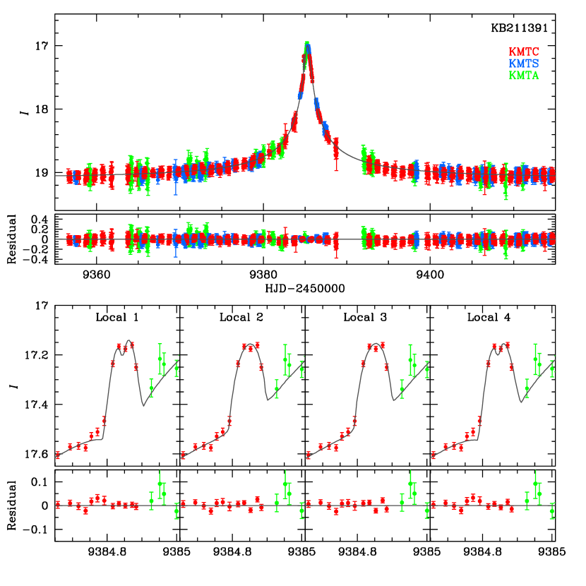
Figure 1: Top panel: Light curve and model for KMT-2021-BLG-1391, color-coded by observatory. Bottom Panels: Zooms of 0.35 days centered on the “bump” anomaly traced by 6 KMTC points. The small-$\rho$ “double-peaked” Local 1 is preferred over either of the large-$\rho$ models (Locals 2 and 3) by $\Delta\chi^{2}=5$, mainly because it better accounts for the “flat top” or possible “dimple” in the bump. See Figure 2.

The overwhelming majority of the light curve (Figure 1) follows a standard 1L1S profile, with $(t_{0},u_{0},t_{\rm E})\simeq(9385.29,0.012,32\,{\rm day})$. However, within hours of the posting of the pipeline reductions, following the alert, a short bump was noted, with center $\Delta t_{\rm anom}=-0.45\,$day prior to $t_{0}$, full width $\Delta t_{\rm bump}=0.11\,$day, and height $\Delta I=0.33\,$mag.

3.2.1 Heuristic Analysis

The anomaly is at $\tau_{\rm anom}=\Delta t_{\rm anom}/t_{\rm E}=-0.014$ and hence $u_{\rm anom}=\sqrt{\tau_{\rm anom}^{2}+u_{0}^{2}}=0.018$, i.e., at very high magnification where planet sensitivity via central and resonant caustics is high (Griest & Safizadeh, 1998). Therefore, an important class of models that may explain this bump anomaly is that the source has passed over a linear structure that extends from a cusp of a central or resonant caustic (on the major image side), or over two very close caustics lying inside such a cusp. In both of these cases, application of the heuristic formalism of Section 3.1 yields,

$$\qquad s_{+}^{\dagger}=1.009.$$ (12)

If the bump were formed by the source passing over a single-peak ridge, it would rise and then fall, both monotonically. In this case, $\rho=\Delta t_{\rm bump}(\sin\alpha)/2t_{\rm E}=1.3\times 10^{-3}$. In fact, the bump is flat-topped, or perhaps has a slight dimple near its peak, which would favor the source crossing two nearly aligned caustics just inside a cusp that are separated by of order the source diameter. In this case, $\rho$ would be approximately half as big, i.e., $\rho\sim 0.65\times 10^{-3}$.

3.2.2 Static Analysis

We ultimately identified 4 solutions via a process that we describe at the end of this subsection. We label these as Locals 1–4. They are illustrated in Figure 1, and their parameters are given in Table 2.

In this and all tables in this paper, we generally present the median and 68% confidence intervals for all quantities except where otherwise specified. We present asymmetric intervals (in $A_{-B}^{+C}$ format) only when the upper and lower excursions differ by more than 20%. Otherwise, we symmetrize the interval (in $A\pm B$ format) to avoid clutter. We always present the mean and standard deviation of $\log q$ in order to aid in understanding whether this quantity is sufficiently well constrained to be included in mass-ratio studies. In this case, the range of means spans 0.12 dex (i.e., about 30%) and their standard deviations are substantially less, indicating that $q$ is well determined.

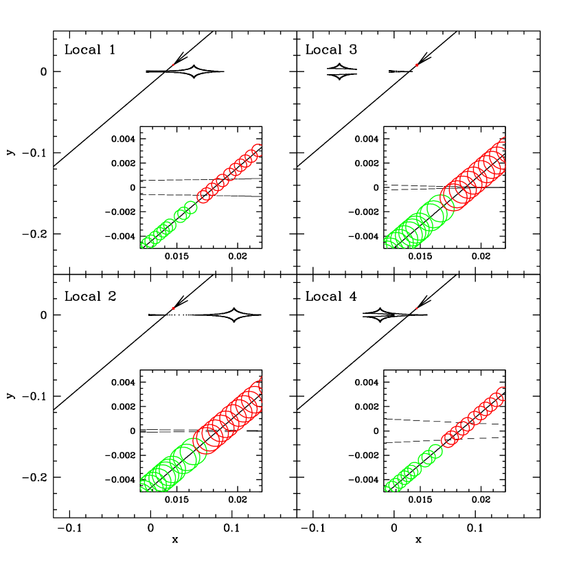
Figure 2: Caustic structures for KMT-2021-BLG-1391 for the two “inner/outer” pairs of degenerate solutions, i.e., Locals 1 & 4 and Locals 2 & 3, respectively. The source size is to scale and the epochs of the observations are shown, with red points from KMTC and green points from KMTA. In the first pair of solutions, the source diameter is slightly smaller than the caustic separation, giving rise to a “dimple” over the peak of the anomaly. See Figure 1. In the second, the source is much larger than the caustic separation. The two pairs of solutions predict very different proper motions and so can ultimately be distinguished by late-time AO imaging.

We can compare these four solutions to those predicted by the heuristic analysis in Section 3.2.1. Regarding $\alpha$, all four models are nearly identical to the prediction. From Table 2, we see that there are two pairs of solutions: Locals 1 and 4, have $(s^{\dagger},\Delta\ln s)_{1,4}=(1.009,0.018)$, while the other pair, Locals 2 and 3, have $(s^{\dagger},\Delta\ln s)_{2,3}=(1.010,0.045)$. That is, each pair has nearly identical $s^{\dagger}$ to the heuristic prediction, but $\Delta\ln s$ is nearly 3 times larger for the second pair. The biggest difference between the two pairs is that $\rho$ is close to twice larger for the second pair. That is, the first pair corresponds to the scenario in which the source crosses two caustics separated by roughly the source diameter, while the second corresponds to the caustic spacing being small compared to the source. See Figure 2.

The first pair is preferred in the sense that it better matches the “dimple” at the midpoint of the anomaly. However, Local 1 predicts a slight pre-caustic depression that is not seen the data, whereas Locals 2 and 3 do not. Moreover, the $\Delta\chi^{2}=5$ difference between Local 1 and either Local 2 or Local 3 reminds us that the advantage of Local 1 is marginal. In any case, both pairs have similar values of $q\sim 4\times 10^{-5}$, and all 4 solutions have even more similar values of $s$. The main difference between the two pairs is in the value of $\rho$, which will propagate to factor $\sim 2$ differences in $\theta_{\rm E}=\theta_{*}/\rho$ and $\mu_{\rm rel}=\theta_{\rm E}/t_{\rm E}$, which we estimate in Section 4.1.

We find that 1L2S solutions are excluded at $\Delta\chi^{2}=94.8$.

The fact that there are two pairs of degenerate solution, rather than one, dawned on us very slowly in the course of preparing this paper. We briefly summarize this process as it may help in the recognition of multiple degeneracies in other events.

Originally, the grid search yielded Locals 1 and 3, as well as a third solution that was discarded after refinement because it had $\Delta\chi^{2}\sim 50$ and was a poor fit by eye. We identified the remaining two solutions (Locals 1 and 3, respectively) as an “inner/outer” degeneracy based partly on the morphology shown in Figure 2 and partly on the fact that the two Locals have $s_{1}>1$ and $s_{3}<1$, respectively. Nevertheless, in the version just prior to submission, we explicitly noted that it was puzzling that the geometric mean $s$ for these two solutions, $\sqrt{s_{1}s_{3}}=0.996$, was less than unity, even though the anomaly was clearly a major-image perturbation. Our concern about this tiny discrepancy, $|\sqrt{s_{1}s_{3}}-s^{\dagger}_{+}|\sim 0.01$, was motivated by accumulating experience that such “large” discrepancies were actually quite rare. (It was a similarly “large” discrepancy that led Gould et al. (2022, in prep) to realize that $s^{\dagger}$ should be regarded as the geometric mean, not the arithmetic mean.)

Then, in the course of final review before submission, JCY argued that the fact that Locals 1 and 3 had substantially different $\rho$ meant that they could not be an inner/outer (or close/wide) degeneracy. In particular, by this time, we already had the example of KMT-2021-BLG-1253, which has a similar 4-fold degeneracy, comprised of two pairs with different $\rho$, which was discovered by a completely different route. See Section 3.3. We then seeded Local 4 with the Local 1 solution (but $s_{4}=(s^{\dagger}_{+})^{2}/s_{1}$) and Local 2 with the Local 3 solution (but $s_{2}=(s^{\dagger}_{+})^{2}/s_{3}$) to find the solutions shown in Table 2. We discuss some further possible implications in Section 6.

3.2.3 Parallax Analysis

Formally, we find a $\Delta\chi^{2}=13.5$ improvement when we add the four parameters ${\mbox{\boldmath$\pi$}}_{\rm E}$ and $\gamma$. However, there is very strong evidence that this “measurement” is due to low-level systematics rather than real physical effects. First, even if the errors were truly Gaussian, the probability of such a $\Delta\chi^{2}$ for four degrees of freedom (dof) would be $p=(1+\Delta\chi^{2}/2)\exp(-\Delta\chi^{2}/2)=1\%$. In itself, this would be regarded as strong, but not overwhelming evidence for the measurement. Second, however, the plots of cumulative $\Delta\chi^{2}$ with time for the three observatories (not shown) are not consistent with each other, demonstrating that the assumption of Gaussian statistics is too strong. Third, the derived parallax values are very high, $\pi_{\rm E}\sim 4$. In Section 4.1, we will show that either $\theta_{\rm E}\sim 0.5\,{\rm mas}$ or $\theta_{\rm E}\sim 0.25\,{\rm mas}$. This parallax determination would then imply $(M,D_{L})\sim(16\,M_{\rm jupiter},0.5\,{\rm kpc})$ or $(M,D_{L})\sim(8\,M_{\rm jupiter},1\,{\rm kpc})$. The prior probability of such nearby lenses is extremely small and would by itself counterbalance the above $p=1\%$, even if Gaussian statistics applied. Further, the prior probability for such low-mass free-floating-planet-like objects (with Earth-mass moons!) is also very low. Finally, the parallax signal comes from the wings of the event, where (because of the faint source, $I\sim 22$) the statistical errors are much larger than the difference fluxes. This is a regime where low-level red noise can easily give rise to spurious signals. We therefore adopt the static solutions.

3.3 KMT-2021-BLG-1253

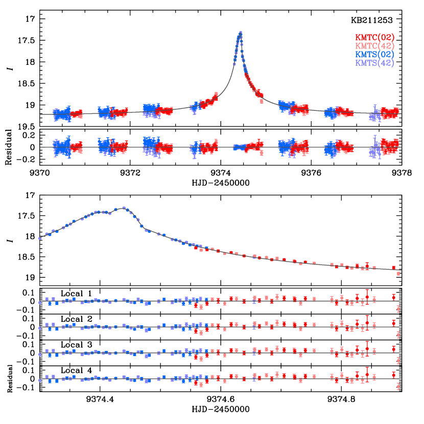
Figure 3: Light curve and models for KMT-2021-BLG-1253. Despite good coverage of the “bump” anomaly, there are four models that fit the data almost equally well (residuals in lower panels). However, all four solutions have similar planet-host mass ratios $q\sim 2.4\times 10^{-4}$ and normalized planet-host separations $s\sim 1$. Nevertheless, they have very different normalized source sizes. See Table 3 and Figure 4.

The majority of the light curve (Figure 3) follows a standard 1L1S profile, with $(t_{0},u_{0},t_{\rm E})\simeq(9374.41,0.006,9\,{\rm day})$. However, just after peak, there is a short bump, with center $\Delta t_{\rm anom}=+0.035\,$day after $t_{0}$, full width $\Delta t_{\rm bump}=0.057\,$day, and height $\Delta I=0.26\,$mag.

3.3.1 Heuristic Analysis

The anomaly is at $\tau_{\rm anom}=\Delta t_{\rm anom}/t_{\rm E}=0.0039$ and hence $u_{\rm anom}=\sqrt{\tau_{\rm anom}^{2}+u_{0}^{2}}=0.0071$, i.e., at very high magnification. Thus, similarly to KMT-2021-BLG-1391, we expect that this bump anomaly may be explained by the source passing over a linear structure that extends from a cusp of a central or resonant caustic on the major image side, or over two very close caustics lying inside such a cusp. Applying the heuristic formalism of Section 3.1, we obtain,

$$\alpha=57^{\circ};\qquad s_{+}^{\dagger}=1.004.$$ (13)

As with KMT-2021-BLG-1391, if the source crosses a cusp, then we expect $\rho\sim\Delta t_{\rm bump}\sin\alpha/2t_{\rm E}=2.6\times 10^{-3}$, while it should be half this value, $\rho\sim 1.3\times 10^{-3}$, if the source crosses a pair of closely spaced caustics.

3.3.2 Static Analysis

The initial grid search yields four solutions. After refining these, we find that one of these solutions is disfavored by $\Delta\chi^{2}=63$ and also appears by eye to be a poor fit to the data. We therefore do not further consider it. We notice that one pair of solutions (called “Local 1” and “Local 2”) are very nearby in $(s,q)$, which raises the concern that they might not be truly distinct. To address this, we run a “hot chain” (i.e., artificially increase the error bars) so that the chain will move easily between minima. We then find that these two solutions have a strong ($\Delta\chi^{2}\sim 15$) barrier between them, so they are indeed distinct. Note, however, that if this event had been in a $\Gamma=1\,{\rm hr}^{-1}$ cadence field, the barrier would have been four times smaller, which would have implied semi-merged minima. After applying a similar hot chain to Local 3, we find a fourth solution, which is a very localized and fairly weak minimum. This emphasizes the importance of running such hot chains, particularly on solutions that have resonant and near-resonant topologies, for which there can be multiple caustic/trajectory geometries that produce similar light curves. Note that if the original grid search had not identified Local 1, then only hot chains that were carried out as a matter of “due diligence” would have uncovered the extra solutions.

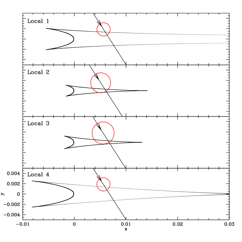
Figure 4: Caustics for KMT-2021-BLG-1253. There are two pairs of solutions: in Locals 1 and 4, the flat-topped bump is explained by a source whose diameter is about equal to the separation between two caustic walls, whereas in Locals 1 and 3, it is explained by a source that is much larger than this separation (and the caustic is substantially smaller). Each pair constitutes a classic wide/close degeneracy. The different normalized source sizes ($\rho\sim 1.3\times 10^{-3}$ vs. $\rho\sim 2\times 10^{-3}$) lead to different Bayesian mass and distance estimates, but these will ultimately be resolved by AO followup observations. See Section 5.2.

From Table 3, we see that the pair, Locals 1 and 4, have $(s^{\dagger},\Delta\ln s)_{1,4}=(1.004,0.068)$, while the pair, Locals 2 and 3, have $(s^{\dagger},\Delta\ln s)_{2,3}=(1.002,0.138)$. That is, both have the $s^{\dagger}\simeq s^{\dagger}_{+}$ that was predicted by the heuristic analysis, but with $\Delta\ln s$ values that differ by a factor 2 from each other. The former set of solutions have $\rho\sim 1.3\times 10^{-3}$, in good agreement with the prediction for the source crossing a close pair of caustics, while the latter have much larger $\rho\sim 2.0\times 10^{-3}$, in qualitative agreement with the prediction for a cusp-crossing geometry. See Figure 4. All four solutions have trajectory angles $\alpha$ in good agreement with the heuristic analysis.

All four solutions have $q\simeq 2.3\times 10^{-4}$ (within errors), and they also have qualitatively similar $s$. As was the case for KMT-2021-BLG-1391, the main difference is in the values of $\rho$, which vary by about a factor 1.5 among the solutions and will propagate into similar differences in $\theta_{\rm E}$ and $\mu_{\rm rel}$.

We find that 1L2S solutions are excluded at $\Delta\chi^{2}=69.9$.

3.3.3 Parallax Analysis

Given the event’s very short timescale ($t_{\rm E}\sim 9\,$days) and very faint source $I_{s}\sim 23.2$, the difference fluxes are below the statistical errors even three days from the peak. The annual parallax signal is negligible on such short timescales, so we do not attempt a parallax measurement, and we therefore adopt the static solutions.

3.4 KMT-2021-BLG-1372

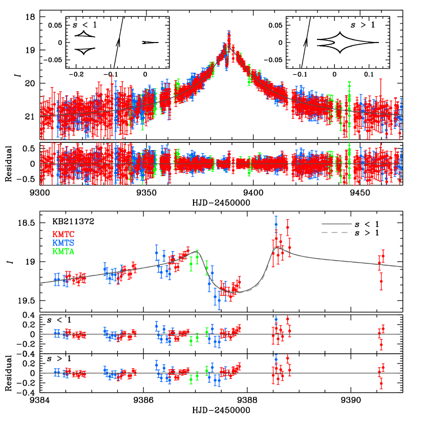
Figure 5: Light curve and model for KMT-2021-BLG-1372. The light curve shows a rounded dip, which is the classic signature of a minor-image perturbation for which the source misses the two planetary caustics. The anomaly is near peak, implying that the trajectory is roughly perpendicular to the planet-host axis and that there should be a classic “inner/outer” degeneracy (Gaudi & Gould, 1997). These expectations are confirmed by the caustic structures shown in the insets.

The light curve (Figure 5) mostly follows a 1L1S profile $(t_{0},u_{0},t_{\rm E})\simeq(9388.8,0.075,71\,{\rm days})$, with the dip of about 0.5 mag, lasting about $\Delta t_{\rm dip}=1.5\,$days, centered at $t_{\rm dip}=9387.70$.

3.4.1 Heuristic Analysis

Noting that $\tau_{\rm anom}=(t_{\rm anom}-t_{0})/t_{\rm E}=-0.015$, the heuristic formalism of Section 3.1 implies,

$$\alpha=282^{\circ};\qquad s_{-}^{\dagger}=0.962;\qquad q\sim 3.4\times 10^{-4}.$$ (14)

3.4.2 Static Analysis

The grid search returns two solutions, which after refinement, yield $(s^{\dagger},\Delta\ln s)=(0.963,0.048)$ and $\alpha=281^{\circ}$, in excellent agreement with the heuristic prediction, while the values of $q\simeq 4.3\times 10^{-4}$ are in good agreement. See Table 4.

We note that there is an extraordinarily bright ($G=9.0$, $J=6.1$) star about $23^{\prime\prime}$ from the event whose diffraction spikes create some difficulties for the photometry. We find that, for KMTC, pyDIA handles these difficulties better than pySIS. Hence, we use pyDIA, and this is the system that we quote in Table 4.

3.4.3 Parallax Analysis

Motivated by the long timescale ($t_{\rm E}\sim 70\,$days), we attempt to measure the microlens parallax and, as usual begin by including orbital motion in the fit. However, we find that neither is usefully constrained in the joint fit and even when we suppress the orbital degrees of freedom, the parallax is still not usefully constrained. As parallax is mostly constrained from the wings of the light curve where the source is only slightly magnified relative to its baseline value $I_{S}\sim 22$, the faintness of the source is likely the origin of the difficulty of making the parallax measurement, possibly compounded by the diffraction spikes. In any case, we adopt the static analysis of Section 3.4.2.

3.5 KMT-2021-BLG-0748

The light curve follows a low-magnification 1L1S profile, $(t_{0},u_{0},t_{\rm E})=(9344.6,0.39,41\,{\rm days})$, except for a short bump represented by three points centered at $t_{\rm bump}\simeq 9346.65$. The three points span only 3.6 hours, but the bump is confined to a total of $\Delta t_{\rm bump}<8.6\,$hours by two flanking points. Thus it is reasonably well characterized despite the relatively low nominal cadence of the the field, $\Gamma=0.4\,{\rm hr}^{-1}$.

3.5.1 Heuristic Analysis

The heuristic formalism yields

$$\alpha=83^{\circ};\qquad s_{+}^{\dagger}=1.216.$$ (15)

We also obtain $\rho\simeq t_{\rm bump}\sin\alpha/2t_{\rm E}\lesssim 4.3\times 10^{-3}$.

3.5.2 Static Analysis

The grid search appears (see below) to return two solutions, whose parameters, after refinement, are shown as Locals 1 and 2 in Table 5. These have $(s^{\dagger},\Delta\ln s)=(1.228,0.031)$ and $\alpha\simeq 83^{\circ}$, in good agreement with Equation (15).

However, as a matter of due diligence, we run a hot chain at these minima and identify two “satellite solutions”, whose parameters are given in Table 5 as Locals 3 and 4. In retrospect, we noted that these solutions actually do appear in the grid search (not shown), but because they have substantially worse fits ($\Delta\chi^{2}\sim 10$), they tended to appear as extended halos of the two best solutions in the grid display rather than as distinct minima. This again emphasizes the importance of investigating hot chains around identified solutions.

These two additional solutions have similar $\alpha\simeq 84^{\circ}$, but quite different $s^{\dagger}$, i.e., $(s^{\dagger},\Delta\ln s)=(1.446,0.0006)$. More significantly, their mass ratios, $q$ are different by factors of several and their self crossing times $t_{*}\simeq 3.4\,$hr are more than twice those of the best solutions, $t_{*}\simeq 1.5\,$hr.

The latter difference is the key to understanding the relation between the two sets of solutions. In the pair of best solutions, the bump is due to the source crossing two nearly parallel caustics, just inside the inner (or outer) on-axis cusp of the planetary caustic. Hence, $t_{*}$ is about 1/4 of the full duration of the bump. In the satellite solutions, the source crosses the cusp, so $t_{*}$ is about 1/2 the full duration of the bump. To accommodate these different morphologies, both $q$ and $t_{\rm E}$ (and so $u_{0}$ and $I_{S}$) are also affected.

Our basic orientation toward these satellite solutions is that they should be considered as $3\,\sigma$ variations on the best solutions. That is, even though they are topologically isolated in the 7-dimensional space of solutions, they represent normal variations on the best solutions. Therefore, we adopt the parameters of the best solutions for this planet.

Nevertheless, we will show in Section 5.4 how future AO observations can definitively resolve the issue (presumably by rejecting the satellite solutions).

We find that 1L2S solutions are excluded at $\Delta\chi^{2}=273$.

3.5.3 Parallax Analysis

In view of the low amplitude and faint source of this event, we do not attempt a parallax analysis. We therefore adopt the static-model results presented in Section 3.5.2.

4 Source Properties

Our primary aim in analyzing the color-magnitude diagram (CMD) of each event is to measure $\theta_{*}$ and so determine

$$\theta_{\rm E}={\theta_{*}\over\rho};\ \qquad\mu_{\rm rel}={\theta_{\rm E}\over t_{\rm E}}.$$ (16)

We follow the method of Yoo et al. (2004) by first finding the offset of the source from the red clump

$$\Delta[(V-I),I]=[(V-I),I]_{S}-[(V-I),I]_{\rm cl},$$ (17)

where we adopt $(V-I)_{\rm cl,0}=1.06$ from Bensby et al. (2013), and we evaluate $I_{\rm cl,0}$ from Table 1 of Nataf et al. (2013), based on the Galactic longitude of the event. This yields the dereddened color and magnitude of the source

$$[(V-I),I]_{S,0}=[(V-I),I]_{\rm cl,0}+\Delta[(V-I),I].$$ (18)

We transform from $V/I$ to $V/K$ using the $VIK$ color-color relations of Bessell & Brett (1988), and then apply the color/surface-brightness relations of Kervella et al. (2004) to obtain $\theta_{*}$. After propagating the measurement errors, we add 5% to the error in quadrature to take account of systematic errors due to the method as a whole.

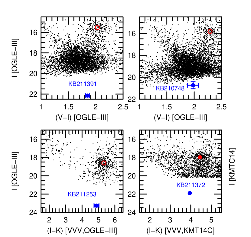
Figure 8: CMDs for each of the four planets reported here. The source positions (blue) and clump-giant centroids (red) are shown for all events.

To obtain $[(V-I),I]_{S}$, we generally begin with pyDIA reductions (Albrow, 2017), which put the light curve and field-star photometry on the same system. We determine $(V-I)_{S}$ by regression of the $V$-band data on the $I$-band data, and we determine $I_{S}$ by regression of the $I$-band data on the best-fit model. When there is calibrated OGLE-III field-star photometry (Szymański et al., 2011), we transform $[(V-I),I]_{s}$ to this system. Otherwise we work in the instrumental KMT pyDIA system, which typically has offsets of $\lesssim 0.2\,$mag from the standard system. The CMDs are shown in Figure 8. When OGLE-III photometry is available, we choose a radius that balances the competing demands of reducing differential extinction and having sufficient density in the clump to measure its centroid.

In only one case (KMT-21-BLG-1391) are we able to make a good measurement of the source color from regression. In the remaining three cases, we estimate this color from the offset of the $I$-band source magnitude relative to the clump. This offset is usually determined (as indicated above) from the clump position found in the $[(V-I),I]$ color-magnitude diagram. However, in two cases (KMT-2021-BLG-1253 and KMT-2021-BLG-1372), we cannot confidently measure the clump position in these optical bands. Therefore, for these cases, we determine $I_{\rm cl}$ from a $[(I-K),I]$ CMD.

The logical chains leading to the $\theta_{*}$ measurements are encapsulated in Table 6. In all cases, the source flux is that of the best solution. Under the assumption of fixed source color, $\theta_{*}$ scales as $10^{-\Delta I_{S}/5}$ for the other solutions, where $\Delta I_{S}$ is the difference in source magnitudes, as given in the Tables of Section 3. The inferred values (or limits upon) $\theta_{\rm E}$, and $\mu_{\rm rel}$ are given in the individual events subsections below, where we also discuss other issues related to the CMDs of each event.

4.1 KMT-2021-BLG-1391

The values of the source flux and resulting $\theta_{*}$ that are given in Table 6 are for Local 1, which is preferred by $\Delta\chi^{2}=5$. We note that for Local 4, $I_{S}$ is fainter by 0.005 mag, implying that $\theta_{*}$ is smaller by 0.2%. This change is far too small to make any difference in the present case. In general, however, the CMD analysis in Table 6 will always give values for the best-fit solution, and $\theta_{*}$ for other solutions can be inferred by $\theta_{*}\propto 10^{-\Delta I/5}$. Then, using the values in Table 2, we find that $\theta_{\rm E}=\theta_{*}/\rho$ and $\mu_{\rm rel}=\theta_{\rm E}/t_{\rm E}$ are given by,

$$\theta_{\rm E}=0.456\pm 0.054\,{\rm mas},\qquad\mu_{\rm rel}=5.26\pm 0.62\,{\rm mas}\,{\rm yr}^{-1},\qquad({\rm Local\ 1}),$$ (19)

$$\theta_{\rm E}=0.226\pm 0.025\,{\rm mas},\qquad\mu_{\rm rel}=2.61\pm 0.29\,{\rm mas}\,{\rm yr}^{-1},\qquad({\rm Local\ 2}).$$ (20)

$$\theta_{\rm E}=0.227\pm 0.025\,{\rm mas},\qquad\mu_{\rm rel}=2.61\pm 0.29\,{\rm mas}\,{\rm yr}^{-1},\qquad({\rm Local\ 3}),$$ (21)

$$\theta_{\rm E}=0.426\pm 0.051\,{\rm mas},\qquad\mu_{\rm rel}=4.90\pm 0.58\,{\rm mas}\,{\rm yr}^{-1},\qquad({\rm Local\ 4}).$$ (22)

We align the position of the source when it was well magnified (so, easily measured) to baseline images taken at the 3.6m Canada-France-Hawaii Telescope (CFHT), in which the $I_{\rm catalog}\sim 19.2$ catalog object appears isolated in $0.5^{\prime\prime}$ seeing. The source position is offset from this object by $0.7^{\prime\prime}$, so it clearly is not associated with the event. There is no obvious object at the position of the source, and there is clearly less flux at this position than from a neighboring star with measured magnitude $I_{\rm neighbor}=21.04\pm 0.14$, while the faintest star detected in the image is $I_{\rm faintest}=21.91$. Hence we can place a firm lower limit on the magnitude of the baseline object, $I_{\rm base}>21$, and therefore on the blend $I_{b}>21.6$. This is a significant constraint: for a lens at the distance of the Galactic bar, this would imply $M_{I}>6.1$, which effectively rules out lenses with $M>0.7\,M_{\odot}$. We will incorporate this flux constraint directly into the Bayesian analysis in Section 5.1.

While we cannot distinguish between the two solutions because $\Delta\chi^{2}$ is only 5, they can ultimately be distinguished based on AO follow-up observations on, e.g., 30m class telescopes, because the two solutions predict very different proper motions. See Section 5.1.

4.2 KMT-2021-BLG-1253

As discussed above, heavy extinction prevents us from measuring $(V-I)_{S}$ from the light curve. Moreover, while the clump can be discerned on the pyDIA CMD (not shown), it is truncated by the $V$-band detection limit, so its centroid cannot be reliably measured. We therefore derive $I_{\rm cl}$ by combining $I$-band data from OGLE-III and $K$-band data from the VVV survey (Minniti et al., 2017) to construct an $[(I-K),K]$ CMD. See Figure 8. After transforming the pyDIA $I_{S}$ measurement to the OGLE-III system, we find that the source lies $\Delta I=4.67$ magnitudes below the clump (see Table 6). Making use of the Hubble Space Telescope (HST) CMD of Baade’s window (Holtzman et al., 1998), we estimate $(V-I)_{0}=0.80\pm 0.10$. In Figure 8, we display the corresponding $(I-K)_{s}$, which we derive from Bessell & Brett (1988) and the observed $(I-K)_{\rm cl}=5.33$ color of the clump. We then proceed as usual.

The values of the source flux and resulting $\theta_{*}$ that are given in Table 6 are for Local 1, which is preferred by just $\Delta\chi^{2}<1.6$ over Local 3 but has a $t_{*}\equiv\rho t_{\rm E}$ that is a factor 0.6 smaller. As in the case of KMT-2021-BLG-1391, the evaluations for the four solutions below reflect the differences in $I_{S}$ as well as in $\rho$:

$$\theta_{\rm E}=0.399\pm 0.062\,{\rm mas},\qquad\mu_{\rm rel}=15.2\pm 2.4\,{\rm mas}\,{\rm yr}^{-1}\qquad{\rm(Local\ 1)},$$ (23)

$$\theta_{\rm E}=0.250\pm 0.036\,{\rm mas},\qquad\mu_{\rm rel}=9.0\pm 1.3\,{\rm mas}\,{\rm yr}^{-1}\qquad{\rm(Local\ 2)},$$ (24)

$$\theta_{\rm E}=0.244\pm 0.034\,{\rm mas},\qquad\mu_{\rm rel}=9.4\pm 1.3\,{\rm mas}\,{\rm yr}^{-1}\qquad{\rm(Local\ 3)},$$ (25)

$$\theta_{\rm E}=0.405\pm 0.063\,{\rm mas},\qquad\mu_{\rm rel}=15.5\pm 2.4\,{\rm mas}\,{\rm yr}^{-1},\qquad{\rm(Local\ 4)}.$$ (26)

The two pairs of solutions predict very different lens-source relative proper motions, $\mu_{\rm rel}$, and they can therefore be distinguished by future AO follow-up observations after elapsed time $\Delta t$, when the lens and source have separated by $\Delta\theta=\mu_{\rm rel}\Delta t$. However, as we discuss in Section 5.2, this will be of less direct interest than in the case of KMT-2021-BLG-1391 because all four solutions have essentially the same mass ratio $q\simeq 2.3\times 10^{-4}$ and normalized projected separation $s\simeq 1$.

As with KMT-2021-BLG-1391, we align the position of the source when it was well magnified to archival images taken at the CFHT. Similarly to that case, the $I_{\rm catalog}\sim 19.4$ catalog object appears relatively isolated in $0.5^{\prime\prime}$ seeing. However, in this case, the source position is offset from the catalog star by $0.49^{\prime\prime}$, meaning that the catalog star somewhat overlaps the source position. The catalog star is just 0.8 mag fainter than the clump, i.e., $>3$ mag brighter than a solar mass main-sequence star in the bulge. Hence, contamination by the catalog star prevents us from placing any useful limits on light from the lens, even in these excellent CFHT images.

4.3 KMT-2021-BLG-1372

Due to high extinction $A_{I}\sim 3.3$ and the relatively faint peak of the event, $I_{\rm peak}\sim 18.4$, we expect roughly $(V-I)_{s}\sim 4.1$ and thus $V_{\rm peak}\sim 22.5$. Therefore, we do not expect to be able to measure $(V-I)_{S}$ and, unfortunately, this proves to be the case. Moreover, the expected position of the clump at $V_{\rm cl}\sim 22$ is too faint to be reliably defined on the $[(V-I),I]$ CMD. Hence, as for KMT-2021-BLG-1253, we carry out the color-magnitude analysis on an $I$ vs. $(I-K)$ CMD. As in that case, we extract $K$-band field star photometry from VVV (Minniti et al., 2017), and we infer the source color from its $I$-band offset relative to the clump. In contrast to the case of KMT-2021-BLG-1253, however, there is no OGLE-III photometry for this field, and we therefore cannot calibrate our KMTC pyDIA photometry. Hence, we report it directly. Nevertheless, this does not pose any great difficulties because, first, our estimates of $\theta_{*}$ depend only on relative photometry, and, second, for the cases that we can perform such calibrations, the typical offset is about $-0.2$ magnitudes. In particular, for the four other events for which we carried out detailed CMD analyses in the preparation of this paper, we find that the mean and standard deviation of this offset are $I_{\rm OGLE-III}-I_{\rm pyDIA,KMTC}=-0.18\pm 0.05$.

Because the source color is not directly measured, we use the offset from the clump, $\Delta I=3.93$, and the Holtzman et al. (1998) HST CMD to estimate $(V-I)_{S,0}=0.75\pm 0.10$.

We obtain only an upper limit on $\rho$, which is better expressed as $t_{*}<0.3\,$day at $2.5\,\sigma$. This arises from the fact that for larger $t_{*}$, the pre-dip “bump” at about HJD${}^{\prime}={\rm HJD}-2450000=9387$ would be washed out. This leads to a limit on the proper motion, $\mu_{\rm rel}>\mu_{\rm lim}=0.84\,{\rm mas}\,{\rm yr}^{-1}$, which is relatively unconstraining. That is, a fraction $p<(\mu_{\rm lim}/\sigma_{\mu})^{3}/6\sqrt{\pi}\rightarrow 2\times 10^{-3}$ of all microlensing events have such low proper motions (Gould et al. 2022, in prep), where we have approximated the bulge proper motion distribution as having a dispersion of $\sigma_{\mu}=2.9\,{\rm mas}\,{\rm yr}^{-1}$ in each direction.

We align 5 archival CFHT images, taken in $0.45^{\prime\prime}$ to $0.5^{\prime\prime}$ seeing to the KMT field, in which the source position is very well determined from high-magnification difference images. We find that the source lies $0.71^{\prime\prime}\pm 0.03^{\prime\prime}$ due west of the $I=21.3$ (KMT system) catalog star, whose monitoring permitted detection of the event. The source position shows no detectable flux, either from the wings of the catalog star or from the source or lens, from which we put a lower limit on the baseline magnitude $I_{\rm base,kmt}>21.8$, i.e., similar to $I_{S}$ (see Table 6). We adopt a conservative limit $I_{L,\rm kmt}\gtrsim 22.5$, which as indicated above (based on the calibrations of other fields), corresponds to $I_{L,\rm calib}\gtrsim 22.3$.

4.4 KMT-2021-BLG-0748

As in the case of KMT-2021-BLG-0748, the $[(V-I),I]$ CMD is well characterized, but the source color $(V-I)_{S}$ cannot be directly measured from regression of the $V$- and $I$-band light curves. The reason for this is similar: The $I$-band flux variation at peak corresponds to a difference magnitude only $\delta I_{\rm peak}=20.3$. Taking account of the extinction and typical source colors, we expect $(V-I)_{S}\sim 2.0$, implying $\delta V_{\rm peak}\sim 22.3$, which is too faint for a reliable measurement. Because the source lies $\Delta I=4.9$ below the clump, we estimate its color using the Holtzman et al. (1998) HST CMD to be $(V-I)_{S,0}=0.83\pm 0.10$.

The two principal solutions have very similar inferred $\theta_{\rm E}$ and $\mu_{\rm rel}$ (differences that are an order of magnitude smaller than their errors), for which we therefore present the average:

$$\theta_{\rm E}=0.32\pm 0.06\,{\rm mas},\qquad\mu_{\rm rel}=2.9\pm 0.6\,{\rm mas}\,{\rm yr}^{-1}\qquad{\rm(Principal\ Solutions\ [L1+L2])}.$$ (27)

Although we do not consider the satellite solutions to be truly independent and believe that their $\chi^{2}$ values should be interpreted at face value, we nonetheless present their corresponding implications in order to guide the interpretation of future AO observations, as discussed in Section 5.4:

$$\theta_{\rm E}=0.16\pm 0.03\,{\rm mas},\qquad\mu_{\rm rel}=2.1\pm 0.3\,{\rm mas}\,{\rm yr}^{-1}\qquad{\rm(Satellite\ Solutions\ [L3+L4])}.$$ (28)

5 Physical Parameters

None of the four planets have sufficient information to precisely specify the host mass and distance. Moreover, several have multiple solutions with significantly different mass ratios $q$ and/or different Einstein radii $\theta_{\rm E}$. For any given solution, we can incorporate Galactic-model priors into standard Bayesian techniques to obtain estimates of the host mass $M_{\rm host}$ and distance $D_{L}$, as well as the planet mass $M_{\rm planet}$ and planet-host projected separation $a_{\perp}$. See Jung et al. (2021) for a description of the Galactic model and Bayesian techniques. However, in most cases we still have to decide how to combine these separate estimates into a single “quotable result”. Moreover, in several cases, we also discuss how the nature of the planetary systems can ultimately be resolved by future AO observations. Hence, we discuss each event separately below.

5.1 KMT-2021-BLG-1391

There are two pairs of solutions whose only major differences are $\rho_{2,3}/\rho_{1,4}=2.0\pm 0.2$ and $q_{2,3}/q_{1,4}=1.28\pm 0.17$. In order to be relevant to both present and future (post AO follow-up) studies, we report five Bayesian results in Table 7, one for each Local and one weighted average. The weighting has two factors. One factor comes from the difference of the $\chi^{2}$ minima of the different Locals. For example, it disfavors Local 2 relative to Local 1 by $\exp(-\Delta\chi^{2}/2)=0.08$. The other comes from the fraction of Bayesian trials that are consistent with the measured parameters $t_{\rm E}$ and $\theta_{\rm E}$, and with the flux constraint. These are (by chance, see below) nearly identical.

As discussed in Section 4.1, there is a strict upper limit on lens flux, $I_{L}>21.6$. We incorporate this limit by assuming that the $A_{I}=1.19$ magnitudes of extinction along the line of sight (see Table 6), are generated by a dust profile with an $h=120\,$pc scale height. The flux constraint eliminates more statistical weight from Locals 1 and 4 simulations because they have higher $\theta_{\rm E}$ and are therefore more populated with the $M\gtrsim 0.7\,M_{\odot}$ lenses that are eliminated by this constraint. This roughly cancels the effect of the higher $\theta_{\rm E}$ (and $\mu_{\rm rel}$), which would otherwise favor these Locals by increasing the available phase space and the cross section.

For present-day studies, we recommend the combined solution for estimates of the physical parameters. The four individual solutions may be useful for comparison with future AO observations that separately resolve the source and lens. As mentioned above, the two pairs of solutions predict very different values of $\mu_{\rm rel}$, which will be decisively measured by future AO observations. In addition, the corresponding $\theta_{\rm E}$ (also very different between the two pairs) and lens flux (and possibly color) must yield a self-consistent lens mass and distance.

We note that if the favored small-$\rho$ solutions are correct, then in 2030 (plausible first AO light for MICADO), the lens and source will be separated by $\Delta\theta\sim 47\pm 6\,{\rm mas}$, while for the disfavored large-$\rho$ solutions, $\Delta\theta\sim 23\pm 3\,{\rm mas}$. In both cases, this is well above the $H$-band FWHM$\sim 11\,{\rm mas}$ and more so for the $J$ band. Such imaging will be required to accurately determine the host mass. The combination of this mass measurement, together with distinguishing between the two pairs of solutions, will yield either an 8% or 13% error in the planet mass, depending on which solution proves to be correct.

5.2 KMT-2021-BLG-1253

The situation for KMT-2021-BLG-1253 is broadly similar to that of KMT-2021-BLG-1391: there are four solutions whose parameters are similar, with the exception of $\rho$. Also note that the $\chi^{2}$ values differ only modestly among the four solutions. However, in this case, there is no useful limit on lens flux.

We proceed in essentially the same way. Table 7 shows the results for the four separate solutions individually, as well as the combined solution. We note that Locals 1 and 4 are significantly disfavored by their relatively high proper motions combined with relatively small Einstein radii. The former are easily generated for nearby lenses, $D_{L}\lesssim 2\,{\rm kpc}$, but in this case the corresponding $\theta_{\rm E}$ would imply $M\lesssim 0.05\,M_{\odot}$ hosts, which are relatively rare. On the other hand, for bulge-bulge lensing (which often generates such $\theta_{\rm E}$), such high $\mu_{\rm rel}$ are relatively rare.

As in the case of KMT-2021-BLG-1391, future AO observations will decisively distinguish between the high- and low-$\mu_{\rm rel}$ solutions. However, this is of less direct interest in the current case because these two classes of solutions do not differ significantly in $q$. Hence, the principal interest will be (as usual) to measure the lens mass from a combination of the lens flux and the more precisely determined $\theta_{\rm E}$ (from the more precisely measured $\mu_{\rm rel}$, together with $t_{\rm E}$).

Note that while the catalog star is relatively bright ($I\sim 19.4$, likely $K\sim 14$), it is displaced from the lens-source system by $0.5^{\prime\prime}$. Thus, it is unlikely to pose any challenges to detecting the lens with 30m class telescopes, even if the lens proves to be a faint bulge dwarf, $M_{K}\sim 9$ ($K\sim 24$), and so has a contrast ratio of 10,000. However, this issue would need to be carefully considered for current 10m class telescopes.

5.3 KMT-2021-BLG-1372

In this case, the two degenerate solutions are essentially identical, except that they differ in $s$ by about 12%. Hence, the physical parameter estimates in Table 7 are also nearly identical. As mentioned in Section 4.3, we impose two limits (in addition to the $t_{\rm E}$ measurement). First, we impose $t_{*}<0.3\,$day, which we argued is hardly constraining. Second, we impose $I_{L}>22.3$. This also has very little practical effect because of the high extinction, $A_{I}=3.93$ (see Table 6). As a sanity check, we explore the effect of imposing a stronger limit $I_{L}>23$, which might plausibly be inferred from the upper limit on the baseline flux. However, this results in a reduction in the Bayesian mass estimates of only 10%, i.e., 5 times smaller than the uncertainty, which again illustrates that the lens flux constraint is weak. We refrain from imposing this stronger constraint because it is less secure and would have very little effect.

The long timescale of this event ($t_{\rm E}\sim 70\,$days) most likely implies a low proper motion. In the Bayesian analysis, we find $\mu_{\rm rel}=2.75\pm 1.25\,{\rm mas}\,{\rm yr}^{-1}$. Because the lens is likely to be fainter than the source in $I$ and also redder than the source, and because of high-extinction, the AO followup observations should probably be done in $H$ or $K$, for which the FWHM, even on the 39m European ELT (EELT), are respectively, 10 mas and 14 mas. Thus, it is possible, but far from guaranteed that the lens can be separately resolved in, e.g., 2030.

5.4 KMT-2021-BLG-0748

In Table 7, we show the Bayesian estimates of the two principal solutions and also their weighted average. As discussed in Section 4.4, we do not consider the satellite solutions to be independent, and we therefore do not separately display their physical-parameter estimates. We note, however, that if they were included in the weighted average, their contribution would be negligible, being downgraded by $\exp(-\Delta\chi^{2}/2)\sim 0.004$, and by a further factor from the Galactic model, due to their lower proper motions.

Given the relatively low proper motion, $\mu_{\rm rel}\sim 2.9\,{\rm mas}\,{\rm yr}^{-1}$, of even the principal solutions, it will not be possible to separately resolve the lens and source until first AO light on 30m class telescopes. At that point, the principal interest will, as usual, be to measure the lens flux, which when combined with the already measured $\theta_{\rm E}$, will yield the lens mass and distance. However, the AO-based $\mu_{\rm rel}$ measurement will also improve the determination of $\theta_{\rm E}=\mu_{\rm rel}t_{\rm E}$ because $t_{\rm E}$ is much better measured than $\theta_{*}$ (due in part to our inability to directly measure the source color).

In addition, the AO measurement can also more decisively exclude the satellite solutions. While the AO measurement of $\mu_{\rm rel}$ can only marginally distinguish between the predictions of Equations (27) and (28), the source-flux predictions of the two sets of solutions differ by more than a factor 2. While this comparison will be somewhat blurred by the fact that the AO flux measurement will be in an infrared band (whereas the microlensing model estimates are in the $I$ band), the uncertainty induced by the lack of a color measurement will be $<0.2$ mag, i.e., much smaller than the factor 2 difference in flux predictions.

6 Discussion

We have presented solutions and analysis for 4 microlensing planets that were discovered from KMTNet data during the 2021 season, as the events were evolving. In contrast to most previous papers about microlensing planets, our goal is not to highlight the features of the individual discoveries but rather to expedite the publication of all 2021 KMTNet planets in order to enable future statistical studies. There will be several dozen such planets. Hence, this paper constitutes, in the first place, a “down payment” on that effort. In addition to the dozens of planets that have been identified by eye from AlertFinder (Kim et al., 2018b) events, there may be additional planets discovered after the EventFinder (Kim et al., 2018a) search has been completed, and more yet after AnomalyFinder (Zang et al., 2021b) has been run on all events. Hence, we consider it prudent to begin “mass production” of planets quickly.

Although the choice of events was simply to rank order those identified by YHR according to their initial mass-ratio estimates, there are some interesting features of the sample as a whole. First, two of the events (KMT-2021-BLG-1391 and KMT-2021-BLG-1253) suffer from a discrete degeneracy in $\rho$ in which a short bump is explained either by a larger-$\rho$ source that straddles two closely spaced caustics or by a smaller-$\rho$ source that successively passes two caustics that are separated by roughly one source diameter. The case of KMT-2021-BLG-1253 is particularly striking because (in contrast to KMT-2021-BLG-1391) there are no identifiable features that could have qualitatively distinguished between the two models if there had been more data. To our knowledge this is the first report of this degeneracy. In any case, it is certainly not so common that we would have expected 2 examples in a random sample of 4 events. This “high rate” may be just due to chance, but it could also indicate that alternate solutions have been missed in past events. In both cases, the different values of $\rho$ lead to very different proper motions. Hence the degeneracy can be broken by future AO observations that separately resolve the lens and source.

This paper is the first to adopt the orientation that essentially all of the planets being reported now can yield mass (rather than mass ratio) measurements in less than a decade and therefore to provide systematic support and guidance for such observations. The first case of source-lens resolution was made more than 20 years ago (Alcock et al., 2001), and there has been a steady stream of such measurements for microlensing planets over the past 7 years (Bennett et al., 2015, 2020; Batista et al., 2015; Bhattacharya et al., 2019; Vandorou et al., 2020) However, these measurements have so far been guided by a strategy focused on the relatively rare events with sufficiently high proper motion to be resolved by 10m class telescopes, which require at least $\sim 50\,{\rm mas}$ separation. Indeed, Henderson et al. (2014) specifically advocated such a strategy. However, with the prospect of 30m class telescopes, the situation is now radically altered. First, the delay time for typical events to be sufficiently separated is reduced from 10–20 years to 3–5 years. Second, this implies that almost all planets that have been discovered or are currently being discovered can be resolved at first 30m AO light, whether they have typical or fairly slow proper motions, and therefore, third, are very likely to be resolvable even if there is no proper motion measurement from the light curve. Fourth, complete samples of planets are likely to include many planets without proper-motion (so, without $\theta_{\rm E}$) measurements (Zhu et al., 2014), which have been regarded as less interesting (so, less frequently published). With AO observations, these planets would gain host mass and planet mass measurements of similar quality to those of planets with $\theta_{\rm E}$ measurements that are derived from the light curve. Thus, the entire field of microlensing planets is likely to be completely transformed by the advent of 30m AO. For this reason, we have given considerable attention to providing information and guidance to such observations.

Table 1: Event Names, Cadences, Alerts, and Locations

Name	$\Gamma\,({\rm hr}^{-1})$	Alert Date	RAJ2000	DecJ2000	$l$	$b$
KMT-2021-BLG-1391	3.0	21 Jun 2021	18:02:44.06	$-28$:03:37.80	$+2.66$	$-2.80$
KMT-2021-BLG-1253	4.0	10 Jun 2021	17:50:28.13	$-29$:16:45.41	$+0.26$	$-1.08$
KMT-2021-BLG-1372	1.0	17 Jun 2021	17:37:57.25	$-28$:08:54.20	$-0.21$	$+1.85$
KMT-2021-BLG-0748	0.4	10 May 2021	18:09:41.12	$-25$:44:47.69	$+5.44$	$-3.03$

Table 2: Microlens Parameters for KMT-2021-BLG-1391

Parameters	Local 1	Local 2	Local 3	Local 4
$\chi^{2}/\rm{dof}$	4255.157/4249	4260.261/4249	4260.229/4249	4258.723/4249
$t_{0}-2459380$	5.291 $\pm$ 0.002	5.291 $\pm$ 0.002	5.291 $\pm$ 0.002	5.290 $\pm$ 0.002
$u_{0}$	0.012 $\pm$ 0.001	0.012 $\pm$ 0.001	0.012 $\pm$ 0.001	0.012 $\pm$ 0.001
$t_{\rm E}$ $(\rm{days})$	31.685 $\pm$ 1.457	31.612 $\pm$ 1.513	31.791 $\pm$ 1.574	31.818 $\pm$ 1.448
$s$	1.027 $\pm$ 0.001	1.056 $\pm$ 0.009	0.966 $\pm$ 0.008	0.991 $\pm$ 0.001
$q$ $(10^{-5})$	3.619 $\pm$ 0.279	4.736 $\pm$ 0.629	$4.635_{-0.549}^{+0.676}$	3.700 $\pm$ 0.302
$\log q$ (mean)	-4.441 $\pm$ 0.034	-4.323 $\pm$ 0.056	-4.332 $\pm$ 0.056	-4.432 $\pm$ 0.036
$\alpha$ $(\rm{rad})$	2.437 $\pm$ 0.004	2.438 $\pm$ 0.004	2.438 $\pm$ 0.004	2.438 $\pm$ 0.004
$\rho$ $(10^{-3})$	0.535 $\pm$ 0.041	1.081 $\pm$ 0.068	1.077 $\pm$ 0.069	0.573 $\pm$ 0.049
$I_{S}$ [KMTC,pySIS]	21.963 $\pm$ 0.052	21.961 $\pm$ 0.054	21.967 $\pm$ 0.056	21.968 $\pm$ 0.052
$I_{B}$ [KMTC,pySIS]	19.159 $\pm$ 0.003	19.159 $\pm$ 0.003	19.159 $\pm$ 0.003	19.159 $\pm$ 0.003
$t_{*}$ $(\rm{hours})$	0.407 $\pm$ 0.025	0.821 $\pm$ 0.031	0.822 $\pm$ 0.031	0.437 $\pm$ 0.030

Table 3: Microlens Parameters for KMT-2021-BLG-1253

Parameters	Local 1	Local 2	Local 3	Local 4
$\chi^{2}/\rm{dof}$	6496.047/6498	6499.627/6498	6497.683/6498	6498.520/6498
$t_{0}-2459370$	4.410 $\pm$ 0.001	4.410 $\pm$ 0.001	4.409 $\pm$ 0.001	4.410 $\pm$ 0.001
$u_{0}$ $(10^{-3})$	5.641 $\pm$ 0.501	$5.373_{-0.489}^{+0.600}$	5.743 $\pm$ 0.510	5.683 $\pm$ 0.553
$t_{\rm E}$ $(\rm{days})$	9.594 $\pm$ 0.841	10.051 $\pm$ 0.989	9.479 $\pm$ 0.814	$9.547_{-0.801}^{+1.025}$
$s$	1.074 $\pm$ 0.004	$1.150_{-0.019}^{+0.027}$	$0.873_{-0.020}^{+0.016}$	0.938 $\pm$ 0.004
$q$ $(10^{-4})$	2.311 $\pm$ 0.261	$2.367_{-0.269}^{+0.334}$	2.523 $\pm$ 0.302	2.282 $\pm$ 0.273
$\log q$ (mean)	-3.637 $\pm$ 0.049	-3.624 $\pm$ 0.055	-3.598 $\pm$ 0.052	-3.643 $\pm$ 0.052
$\alpha$ $(\rm{rad})$	1.002 $\pm$ 0.010	1.003 $\pm$ 0.011	1.002 $\pm$ 0.010	0.999 $\pm$ 0.011
$\rho$ $(10^{-3})$	1.297 $\pm$ 0.145	2.022 $\pm$ 0.211	2.141 $\pm$ 0.197	1.306 $\pm$ 0.166
$I_{S}$ [KMTC,pySIS]	23.185 $\pm$ 0.099	23.240 $\pm$ 0.111	23.171 $\pm$ 0.097	23.179 $\pm$ 0.108
$I_{B}$ [KMTC,pySIS]	19.287 $\pm$ 0.002	$19.286_{-0.002}^{+0.003}$	19.288 $\pm$ 0.002	19.288 $\pm$ 0.003
$t_{*}$ (hours)	$0.297_{-0.017}^{+0.022}$	0.488 $\pm$ 0.014	0.487 $\pm$ 0.015	$0.298_{-0.019}^{+0.027}$

Table 4: Microlens Parameters for KMT-2021-BLG-1372

Parameters	$s<1$	$s>1$
$\chi^{2}/\rm{dof}$	1541.940/1541	1540.605/1541
$t_{0}-2459380$	8.758 $\pm$ 0.055	8.757 $\pm$ 0.057
$u_{0}$	0.074 $\pm$ 0.011	0.075 $\pm$ 0.011
$t_{\rm E}$ $(\rm{days})$	71.937 $\pm$ 9.161	70.665 $\pm$ 8.737
$s$	0.917 $\pm$ 0.006	1.011 $\pm$ 0.008
$q$ $(10^{-4})$	4.175 $\pm$ 0.724	4.419 $\pm$ 0.715
$\log q$ (mean)	-3.386 $\pm$ 0.080	-3.361 $\pm$ 0.075
$\alpha$ $(\rm{rad})$	4.896 $\pm$ 0.015	4.896 $\pm$ 0.015
$\rho$ $(10^{-4})$	$<42$	$<42$
$I_{S}$ [KMTC,pyDIA]	21.919 $\pm$ 0.158	21.897 $\pm$ 0.156
$I_{B}$ [KMTC,pyDIA]	$21.750_{-0.083}^{+0.105}$	$21.762_{-0.087}^{+0.107}$
$t_{*}$ $(\rm{hours})$	$0.184_{-0.165}^{+1.322}$	$0.148_{-0.129}^{+1.180}$
$t_{*}$ $(\rm{days})$	$<0.3$	$<0.3$

Note. — Limits on $\rho$ and $t_{*}=\rho t_{\rm E}$ are at $2.5\,\sigma$.

Table 5: Microlens Parameters for KMT-2021-BLG-0748

Parameters	Local 1	Local 2	Local 3	Local 4
$\chi^{2}/\rm{dof}$	654.966/655	655.837/655	665.440/655	664.390/655
$t_{0}-2459340$	4.684 $\pm$ 0.408	4.647 $\pm$ 0.398	4.685 $\pm$ 0.395	4.620 $\pm$ 0.384
$u_{0}$	$0.411_{-0.063}^{+0.120}$	0.402 $\pm$ 0.060	0.737 $\pm$ 0.082	0.760 $\pm$ 0.078
$t_{\rm E}$ $(\rm{days})$	39.756 $\pm$ 5.871	41.116 $\pm$ 4.581	27.880 $\pm$ 2.193	27.459 $\pm$ 2.018
$s$	$1.267_{-0.033}^{+0.060}$	1.190 $\pm$ 0.042	1.455 $\pm$ 0.051	1.438 $\pm$ 0.057
$q$ $(10^{-3})$	1.261 $\pm$ 0.429	$1.078_{-0.233}^{+0.304}$	0.597 $\pm$ 0.179	0.491 $\pm$ 0.148
$\log q$ (mean)	-2.913 $\pm$ 0.155	-2.968 $\pm$ 0.107	-3.232 $\pm$ 0.135	-3.316 $\pm$ 0.134
$\alpha$ $(\rm{rad})$	1.451 $\pm$ 0.029	1.449 $\pm$ 0.025	1.474 $\pm$ 0.019	1.473 $\pm$ 0.018
$\rho$ $(10^{-3})$	1.523 $\pm$ 0.525	$1.506_{-0.482}^{+0.356}$	5.037 $\pm$ 0.535	5.067 $\pm$ 0.469
$I_{S}$ [KMTC,pySIS]	$20.796_{-0.394}^{+0.244}$	20.843 $\pm$ 0.226	19.867 $\pm$ 0.208	19.814 $\pm$ 0.198
$I_{B}$ [KMTC,pySIS]	$17.862_{-0.014}^{+0.032}$	17.859 $\pm$ 0.014	$17.964_{-0.032}^{+0.040}$	17.973 $\pm$ 0.036
$t_{*}$ (hours)	$1.534_{-0.623}^{+0.305}$	$1.522_{-0.500}^{+0.278}$	3.373 $\pm$ 0.197	3.339 $\pm$ 0.174

Table 6: CMD Parameters for Five 2021 Planets

Parameter	KB211391	KB211253	KB211372	KB210748
$(V-I)_{\rm s}$	1.85$\pm$0.04	N.A.	N.A.	N.A.
$(V-I)_{\rm cl}$	2.03$\pm$0.02	N.A.	N.A.	2.29$\pm$0.02
$(V-I)_{\rm cl,0}$	1.06	1.06	1.06	1.06
$(V-I)_{\rm s,0}$	0.88$\pm 0.05$	0.80$\pm$0.10	0.75$\pm$0.10	0.83$\pm$0.10
$I_{\rm s}$	22.15$\pm$0.05	23.27$\pm$0.10	21.90$\pm$ 0.16	20.73$\pm$0.32
$I_{\rm cl}$	15.55$\pm$0.03	18.60$\pm$0.03	17.97$\pm$0.05	15.83$\pm$0.05
$I_{\rm cl,0}$	14.36	14.43	14.46	14.29
$I_{\rm s,0}$	20.96$\pm$0.06	19.10$\pm$0.10	18.39$\pm$0.16	19.19$\pm$0.32
$\theta_{*}$ ($\mu{\rm as}$)	0.244$\pm 0.023$	0.517$\pm$0.072	0.692$\pm$0.097	0.514$\pm$0.089

Note. — Event names are abbreviations for, e.g., KMT-2021-BLG-1391.

Table 7: Physical properties

Event						Relative Weights
Models	Physical Properties					Gal.Mod.	$\chi^{2}$
KB211391	$M_{\rm host}$ $[M_{\sun}]$	$M_{\rm planet}$ $[M_{\earth}]$	$D_{\rm L}$ [kpc]	$a_{\bot}$ [au]
Local 1	0.39 $\pm$ 0.19	4.67 $\pm$ 2.25	$5.55_{-1.65}^{+1.08}$	$2.41_{-0.65}^{+0.50}$		0.919	1.000
Local 2	$0.23_{-0.12}^{+0.20}$	$3.57_{-1.83}^{+3.17}$	$6.72_{-1.15}^{+0.94}$	1.63 $\pm$ 0.34		0.938	0.078
Local 3	$0.23_{-0.12}^{+0.20}$	$3.52_{-1.80}^{+3.11}$	$6.72_{-1.15}^{+0.94}$	1.49 $\pm$ 0.31		0.928	0.079
Local 4	0.38 $\pm$ 0.19	4.67 $\pm$ 2.31	$5.76_{-1.63}^{+1.03}$	$2.26_{-0.59}^{+0.48}$		1.000	0.168
Total	0.37 $\pm$ 0.19	4.55 $\pm$ 2.31	$5.72_{-1.67}^{+1.10}$	$2.29_{-0.71}^{+0.56}$
KB211253	$M_{\rm host}$ $[M_{\sun}]$	$M_{\rm planet}$ $[M_{\earth}]$	$D_{\rm L}$ [kpc]	$a_{\bot}$ [au]
Local 1	$0.290_{-0.15}^{+0.28}$	$22.23_{-11.79}^{+21.19}$	$6.33_{-1.35}^{+1.06}$	1.96 $\pm$ 0.52		0.224	1.000
Local 2	$0.22_{-0.12}^{+0.24}$	$17.42_{-9.18}^{+19.08}$	$6.78_{-1.24}^{+1.00}$	1.76 $\pm$ 0.42		0.937	0.167
Local 3	$0.21_{-0.11}^{+0.23}$	$17.74_{-9.29}^{+19.65}$	$6.78_{-1.23}^{+0.99}$	1.30 $\pm$ 0.30		1.000	0.441
Local 4	$0.29_{-0.15}^{+0.28}$	$22.05_{-11.71}^{+21.07}$	$6.32_{-1.36}^{+1.06}$	1.72 $\pm$ 0.46		0.208	0.290
Adopted	$0.24_{-0.13}^{+0.26}$	$19.05_{-10.14}^{+20.42}$	$6.64_{-1.30}^{+1.03}$	$1.52_{-0.41}^{+0.57}$
KB211372	$M_{\rm host}$ $[M_{\sun}]$	$M_{\rm planet}$ $[M_{\earth}]$	$D_{\rm L}$ [kpc]	$a_{\bot}$ [au]
$s<1$	0.42 $\pm$ 0.25	58.95 $\pm$ 34.51	$5.97_{-2.41}^{+1.49}$	2.22 $\pm$ 0.72		0.959	0.513
$s>1$	0.42 $\pm$ 0.25	62.41 $\pm$ 36.55	$5.97_{-2.41}^{+1.49}$	2.45 $\pm$ 0.79		1.000	1.000
Adopted	0.42 $\pm$ 0.25	61.27 $\pm$ 35.88	$5.97_{-2.41}^{+1.49}$	2.37 $\pm$ 0.77
KB210748	$M_{\rm host}$ $[M_{\sun}]$	$M_{\rm planet}$ $[M_{J}]$	$D_{\rm L}$ [kpc]	$a_{\bot}$ [au]
Local 1	$0.36_{-0.20}^{+0.31}$	$0.47_{-0.26}^{+0.42}$	$6.09_{-1.31}^{+0.91}$	2.46 $\pm$ 0.67		1.000	1.000
Local 2	$0.36_{-0.20}^{+0.32}$	$0.41_{-0.23}^{+0.36}$	$6.10_{-1.32}^{+0.91}$	2.35 $\pm$ 0.64		0.772	0.647
Adopted	$0.36_{-0.20}^{+0.32}$	$0.45_{-0.25}^{+0.40}$	$6.09_{-1.31}^{+0.92}$	2.43 $\pm$ 0.67

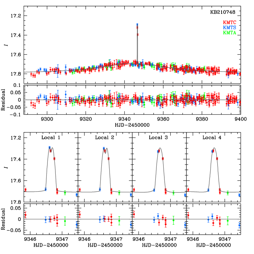
Figure 6: Top panel: Light curve and model for KMT-2021-BLG-0748 color-coded by observatory. Bottom Panel: Four zooms of 1.7 days centered on the “bump” anomaly, which is traced by 3 points. Locals 1 and 2 are preferred by $\Delta\chi^{2}\sim 10$ over Locals 3 and 4 mainly because the overall light-curve normalization favors the first point on the bump (from KMTS) being brighter than the second (from KMTC). Hence, the $\chi^{2}$ difference is not fully reflected in the residuals of the bump region. See Figure 7 for the origin of this difference.

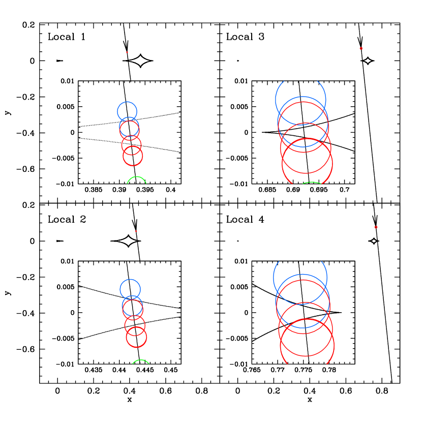
Figure 7: Caustic geometries for the four Locals of KMT-2021-BLG-0748. Locals 1 and 2 are a classic example of the inner/outer degeneracy (Gaudi & Gould, 1997), i.e. the source passes just inside the inner cusp of the planetary caustic in Local 1 and just inside the outer cusp in Local 2. The source is smaller than the caustic separation, which induces “dimples” in the first two zoom panels of Figure 6. Morphologically, Locals 3 and 4 are “satellite” solutions of Locals 1 and 2, in which the source passes closer to the cusp. However, the source is about 3 times larger, which induces smooth bumps (i.e., no dimples) in the last two zoom panels of Figure 6. And this change induces large changes in $s$ and $q$.

References

- Alard & Lupton (1998) Alard, C. & Lupton, R.H.,1998, ApJ, 503, 325
- Albrow (2017) Albrow, M.D. Michaeldalbrow/Pydia: InitialRelease On Github., vv1.0.0, Zenodo
- Albrow et al. (2009) Albrow, M. D., Horne, K., Bramich, D. M., et al. 2009, MNRAS, 397, 2099
- Alcock et al. (2001) Alcock, C., Alssman, R.A., Alves, D.R., et al. 2001, Nature, 414, 617
- An et al. (2002) An, J.H., Albrow, M.D., Beaulieu, J.-P. et al. 2002, ApJ, 572, 521
- Batista et al. (2011) Batista, V., Gould, A., Dieters, S. et al. A&A, 529, 102
- Batista et al. (2015) Batista, V., Beaulieu, J.-P., Bennett, D.P., et al. 2015, ApJ, 808, 170
- Bennett et al. (2015) Bennett, D.P., Bhattacharya, A., Anderson, J., et al. 2015, ApJ, 808, 169
- Bennett et al. (2020) Bennett, D.P., Bhattacharya, A., Beaulieu, J.-P., et al. 2020, AJ, 159, 68
- Bensby et al. (2013) Bensby, T. Yee, J.C., Feltzing, S. et al. 2013, A&A, 549, A147
- Bessell & Brett (1988) Bessell, M.S., & Brett, J.M. 1988, PASP, 100, 1134
- Bhattacharya et al. (2019) Bhattacharya, A., Beaulieu, J.-P., Bennett, D.P., et al. 2019, AJ, 156, 289
- Chung & Lee (2011) Chung, S.-J. & Lee, C.-U. 2011, MNRAS, 411, 151
- Dong et al. (2009) Dong, S., Gould, A., Udalski, A., et al. 2009, ApJ, 695, 970
- Gaudi & Gould (1997) Gaudi, B.S. & Gould, A. 1997, ApJ, 486, 85
- Gaudi et al. (2002) Gaudi, B.S., Albrow, M.D., An, J. 2002, ApJ, 566, 463
- Gould (1992) Gould, A. 1992, ApJ, 392, 442
- Gould (2000) Gould, A. 2000, ApJ, 542, 785
- Gould (2004) Gould, A. 2004, ApJ, 606, 319
- Gould & Loeb (1992) Gould, A. & Loeb, A. 1992, ApJ, 396, 104
- Gould et al. (2010) Gould, A., Dong, S., Bennett, D.P. et al. 2010, ApJ, 710, 1800
- Griest & Safizadeh (1998) Griest, K. & Safizadeh, N. 1998, ApJ, 500, 37
- Henderson et al. (2014) Henderson, C.B., Park, H., Sumi, T., et al. 2014, ApJ, 794, 71
- Herrera-Martin et al. (2020) Herrera-Martin, A., Albrow, A., Udalski, A., et al. 2020, AJ, 159, 134
- Holtzman et al. (1998) Holtzman, J.A., Watson, A.M., Baum, W.A., et al. 1998, AJ, 115, 1946
- Hwang et al. (2018) Hwang, K.-H., Udalski, A., Shvartzvald, Y. et al. 2018, AJ, 155, 20
- Hwang et al. (2021) Hwang, K.-H., Zang, W., Gould, A., et al.., 2021, AJ, in press, arXiv:2106.06686
- Jung et al. (2021) Jung, Y. K., Han, C., Udalski, A.,. et al. 2021, AJ, 161, 293
- Kervella et al. (2004) Kervella, P., Thévenin, F., Di Folco, E., & Ségransan, D. 2004, A&A, 426, 297
- Kim et al. (2016) Kim, S.-L., Lee, C.-U., Park, B.-G., et al. 2016, JKAS, 49, 37
- Kim et al. (2018a) Kim, D.-J., Kim, H.-W., Hwang, K.-H., et al., 2018a, AJ, 155, 76
- Kim et al. (2018b) Kim, D.-J., Hwang, K.-H., Shvartzvald, et al. 2018b, arXiv:1806.07545
- Minniti et al. (2017) Minniti, D., Lucas, P., VVV Team, 2017, yCAT 2348, 0
- Nataf et al. (2013) Nataf, D.M., Gould, A., Fouqué, P. et al. 2013, ApJ, 769, 88
- Paczyński (1986) Paczyński, B. 1986, ApJ, 304, 1
- Skowron et al. (2011) Skowron, J., Udalski, A., Gould, A et al. 2011, ApJ, 738, 87
- Szymański et al. (2011) Szymański, M.K., Udalski, A., Soszyński, I., et al. 2011, Acta Astron., 61, 83
- Tomaney & Crotts (1996) Tomaney, A.B. & Crotts, A.P.S. 1996, au, 112, 2872
- Udalski et al. (2005) Udalski, A., Jaroszyński, M., Paczyński, B, et al. 2005, ApJ, 628, L109.
- Vandorou et al. (2020) Vandorou, A., Bennett, D.P., Beaulieu, J.-P., et al. 2020, AJ, 160, 121
- Wang et al. (2022) Wang, H., Zang, W., Zhu, W, et al. 2022, MNRAS, 510, 1778
- Yee et al. (2012) Yee, J.C., Shvartzvald, Y., Gal-Yam, A. et al. 2012, ApJ, 755, 102
- Yee et al. (2015) Yee, J.C., Gould, A., Beichman, C., 2015, ApJ, 810, 155
- Yee et al. (2021) Yee, J.C., Zang, W., Udalski, A. et al. 2021, AJ, 162, 180
- Yoo et al. (2004) Yoo, J., DePoy, D.L., Gal-Yam, A. et al. 2004, ApJ, 603, 139
- Zang et al. (2021a) Zang, W., Han, C., Kondo, I., et al. 2021a, 2021, RAA, 21, 239
- Zang et al. (2021b) Zang, W., Hwang, K.-H., Udalski, A., et al. 2021b, AJ, 162, 163
- Zhang et al. (2021) Zhang, K., Gaudi, B.S., Bloom, J.S, 2021, arXiv:2111.13696
- Zhu et al. (2014) Zhu, W., Penny, M., Mao, S., Gould, A., & Gendron, R. 2014, ApJ, 788, 73