Network Calculus with Flow Prolongation –
A Feedforward FIFO Analysis enabled by ML

Abstract

The derivation of upper bounds on data flows’ worst-case traversal times is an important task in many application areas. For accurate bounds, model simplifications should be avoided even in large networks. NC provides a modeling framework and different analyses for delay bounding. We investigate the analysis of feedforward networks where all queues implement FIFO service. Correctly considering the effect of data flows onto each other under FIFO is already a challenging task. Yet, the fastest available NC FIFO analysis suffers from limitations resulting in unnecessarily loose bounds. A feature called FP has been shown to improve delay bound accuracy significantly. Unfortunately, FP needs to be executed within the NC FIFO analysis very often and each time it creates an exponentially growing set of alternative networks with prolongations. FP therefore does not scale and has been out of reach for the exhaustive analysis of large networks. We introduce DeepFP, an approach to make FP scale by predicting prolongations using machine learning. In our evaluation, we show that DeepFP can improve results in FIFO networks considerably. Compared to the standard NC FIFO analysis, DeepFP reduces delay bounds by $12.1\text{\,}\mathrm{\char 37\relax}$ on average at negligible additional computational cost.

I Introduction

Modern, newly developed networked systems are often required to provide some kind of minimum performance level. Applications in domains such as the automotive and avionics sector [Geyer2016] as well as factory automation often crucially rely on this minimum performance. Their main focus is then on one important network property: the worst-case traversal time, i.e., the end-to-end delay, of data communication. To that end, safety-critical applications that are crucial for the entire system’s certification need to formally prove guaranteed upper bounds on the end-to-end delay of data flows. A second characteristic of modern networks in these domains is that they are not designed from scratch anymore but derived from IEEE Ethernet. For example, network standards based on Ethernet such as AFDX or IEEE TSN are becoming prevalent. These standards usually follow a simple queueing design, “FIFO per priority queue”. In the NC analysis’ point of view, this is essentially a FIFO system model – a model already hard to analyze without introducing simplifying worst-case assumptions. We even aim at improving the analysis in both dimensions, result accuracy and execution time, by adding the FP feature as well as ML-predictions steering our proposed NC FIFO analysis. Our contribution can be applied to any system designed around FIFO multiplexing and forwarding of data that can be modeled with NC. For example, existing works on NC modeling of the specific schedulers used in AFDX or TSN networks.

NC is a framework with modeling and analysis capabilities. For best results, i.e., tight delay bounds, both parts should be developed in lockstep to prevent mismatches in their respective capabilities. Unfortunately, this has not always been the case. Adding assumptions like FIFO to a system model is naturally easy, yet tracking the property across an entire feedforward network to consider mutual impact of flows is not. Other prominent network properties such as PBOO [LeBoudec2001] and PMOO [Schmitt2008b] stating that data flows do not exhibit stop-and-go behavior nor overtake each other multiple times when crossing a tandem of servers, have found their way into some NC analyses eventually. However, the important PMOO property is not available in the non-FIFO [Rizzo2005, Schmitt2011] analysis and not necessarily considered by the fastest available FIFO analysis [Bisti2008, Bisti2012, Scheffler2021].

If a network property cannot be considered by NC tandem analysis, it is replaced by a worst-case assumption in the analysis’ internal view. Therefore, improvements to NC tandem analyses tried to remove such overly pessimistic assumptions by adding analysis features that improve the computed delay bound. A somewhat different feature was recently presented with FP [Bondorf2017c]. It actively converts the network model given to the NC analysis to a more pessimistic one. This new view is explicitly derived such that a shortcoming of the NC FIFO analysis is circumvented while delay bounds remain valid. It has been shown that this model transformation can simultaneously help implementing the PMOO property to a larger extent [GeyerSchefflerBondorf_RTAS2021].

FP is conceptually straight-forward: assume flows take more hops than they actually do. Nonetheless FP is a powerful feature to add to NC analysis that was adopted in SNC [Nikolaus2020b], too. Finding the best prolongation of flows is prone to a combinatorial explosion. On a tandem with $n$ hops and $m$ flows, there are $O(n^{m})$ alternatives for path prolongation (including the alternative not to prolong any cross-flow). Even with a deep understanding of the NC analysis, the amount could not be reduced significantly to make FP analysis scale [Bondorf2017c].

Additionally, the fast FIFO analysis derives multiple algebraic NC terms, each bounding a single flow’s delay. The amount of terms grows exponentially with the network size and none of them computes the tightest bound independent of flow parameters. I.e., all need to be derived and solved [Bondorf2017a], Thus, the analysis must compute a multitude of delay bounds to find the minimum among them [Bisti2008, Bisti2012]. Adding the FP feature to a FIFO analysis for feedforward networks results in a hardly scalable analysis.

In this article, we present ML approach to overcome exhaustive searches in the algebraic NC FIFO analysis with the FP feature. Put simple, we have trained a GNN to predict the best choices for the analysis’ term creation. This allows the analysis to scale, and can also be extended to multiple predictions per choice. We base our contribution on some previous work [Geyer2019a, Geyer2020, Geyer2020b, GeyerSchefflerBondorf_RTAS2021], presenting here the DeepFP analysis illustrated in Figure 1.

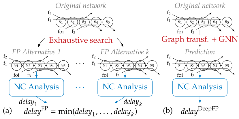
Figure 1: Comparison between the (a) exhaustive FP with $O(n^{m})$ NC analyses and (b) DeepFP with one prediction.

Via numerical evaluations, we show that DeepFP is an efficient and scalable method that reduces NC FIFO delay bound by an average of $12.1\text{\,}\mathrm{\char 37\relax}$ on our test networks. We show that DeepFP scales to networks with up to 500 flows without compromising on tightness, whereas other methods fail to finish within a deadline of $1\text{\,}\mathrm{h}$ and / or a memory limitation of $5\text{\,}\mathrm{G}\mathrm{B}$. Compared to previous work [Geyer2019a, Geyer2020, Geyer2020b, GeyerSchefflerBondorf_RTAS2021], we train DeepFP using a RL approach and show that it even outperforms an expert heuristic for FP on small networks.

This article is organized as follows: Section II presents related work and Section III gives an overview on NC. Section IV shows how FP improves the NC FIFO analysis and the challenges it imposes. Section V contributes our DeepFP, making FP applicable in the network analysis. Section VI evaluates DeepFP and LABEL:sec:conclusion concludes the article.

II Related Work

NC and RTC

NC creates a purely descriptive model of a network of queueing locations and data flows (see Section III-A). The NC analysis then computes a bound on the worst-case delay for a certain flow, the so-called foi (see Section III-B). A variant of NC that focuses on (embedded) real-time systems was established by the RTC [Thiele2000]. Equivalence between the slightly differing resource descriptions has been proven in [Bouillard2009]. What remains is the difference in modeling of the “network” and the analysis thereof. RTC models networks of components such as the Greedy Processing Component (GPC) [Guan2013, Tang2017]. Each component represents a macro, i.e., a fixed sequence of algebraic NC operations to apply to its input. Thus, the model already encodes the analysis. Moreover, this component-based modeling approach mostly restricts the analysis to strict priority multiplexing, yet, efforts to incorporate the PBOO property and the PMOO property can be found in the literature [Lampka2016, Lampka2017, Tang2019]. We, in contrast, aim for a model-independent improvement of the automatic derivation of a valid order of NC operations – the process called NC analysis – for feedforward networks of FIFO queues. First results on this topic in NC [LeBoudec2001, Fidler2004] were refined to the LUDB analysis [Bisti2008, Bisti2012] that we use as the (algebraic) NC FIFO analysis in our work. Later, an entirely different analysis approach was proposed in [Bouillard2012, Bouillard2015]. It converts the NC entire feedforward network model to a single optimization problem, optimizing for the foi’s delay bound. The tight MILP formulation introduces forbiddingly large computational effort such that it was augmented with a less tight LP formulation – we call these analyses FFMILPA and FFLPA. Current efforts in this stream of research further tune the FFLPA’s tradeoff between delay bound tightness and computational effort by adding constraints derived with algebraic NC [Bouillard2022]. We numerically compare DeepFP with FFLPA and FFMILPA in Section VI.

FP in NC

FP was mentioned in [Schmitt2007] to be used for the purpose of complexity reduction of NC analysis. This is achieved if a flow can be prolonged to share the same path as another flow, allowing both to be aggregated within the analysis. In contrast, we pair FP with the (LUDB) NC FIFO analysis for feedforward networks [Scheffler2021] to counteract its main tightness-compromising problem, thus considerably improving delay bounds. There has been one previous mention of FP in FIFO networks: [Bisti2008] briefly shares the observation that, if prolonged, a cross-flow can be aggregated with the foi – which is independent of the problem we tackle in this article. The observation of [Bisti2008] can thus be combined with our contribution. Yet, as it only applies to at most one single point in the analysis, we will focus our article on investigating the FP-improvement throughout the entire feedforward NC FIFO analysis and will leave this smaller feature’s investigation to future work. Prolonging at the front may also be possible in the arbitrary multiplexing PMOO analysis [Bondorf2020].

GNN

GNN were first introduced in [Gori2005] and [Battaglia2018] presents a framework that formalizes many concepts applied in GNN in a unified way. GNN were already proposed as an efficient method for replacing exhaustive searches or similar NP-hard problems such as the traveling salesman problem [Prates2019]. A recent survey [Wang2020] about existing applications of ML to formal verification shows that this combination can accelerate, for instance, theorem proving, model-checking, Boolean satisfiability (SAT) and satisfiability modulo theories (SMT) problems. As we show, NC has been combined with other methods, too.

GNN were first introduced in [Gori2005, Scarselli2009]. a concept subsequently refined in recent works. Gated Graph Neural Networks (GGNN) [Li2016a] extended this architecture with modern practices by using Gated Recurrent Unit (GRU) memory units [Cho2014b]. Message-passing neural network were introduced in [Gilmer2017], with the goal of unifying various GNN and graph convolutional concepts. Finally, [Battaglia2018] introduced the GN framework, a unified formalization of many concepts applied in GNN.

Concrete examples are: [Li2018] that tackles the challenge of solving combinatorial optimization problems using Graph Convolutional Networks. [Selsam2019] addresses constraint satisfaction problems (CSP) and particularly SAT problems using GNN, showing that GNN can be used for such problems, hence, an application to NC is also feasible. [Palm2018] used Recurrent Relational Networks to solve Sudoku problems, and [Prates2019] used GNN to solve the traveling salesman problem. Finally, recent work in [Davies2021] applies GNN to mathematical theorem proving.

For computer networks, GNN have lately been applied to different non-NC performance evaluations of networks [Geyer2018e, Rusek2020, Suzuki2020]. E.g., [Mai2021] used GNN for predicting the feasibility of scheduling configurations in Ethernet networks. Surveys on GNN applications to communication networks and network optimization can be found in [Vesselinova2020, Jiang2022].

NC and GNN

DeepTMA was proposed in [Geyer2019a] as a framework where GNN are used for predicting the best contention model whenever the analysis is faced with alternatives. DeepFP and DeepTMA are closely related in spirit: both methods use a graph transformation and a GNN to replace a computationally expensive exhaustive search. DeepTMA, as it name suggests, does so within the TMA [Bondorf2017a]. TMA does not consider – and for that matter nor trace – the FIFO property but instead replaces it with a worst-case assumption whenever flows multiplex in a queue. That results in a considerably less complex approach that was shown to scale to large feedforward networks with up to $14\,000$ flows [Geyer2020b]. But as shown in [Scheffler2021], TMA-derived delay bounds are overly pessimistic in FIFO networks. In contrast, DeepFP pairs the NC FIFO analysis, including the FP feature, with a GNN. This requires us, among other challenges, to design a new graph transformation and to connect all the parts efficiently.

Various other works using GNN for achieving better delay bounds or optimizing network configurations have been proposed. [Geyer2018d] proposed to predict the delay bound computed by different NC analyses by using GNN. This information can be used to select the analysis that will most likely deliver the best delay bound, i.e., unlike our DeepFP or DeepTMA, the GNN predictions do not impacted the proceeding of the analysis itself. Finally, [Mai2021] recently used GNN for predicting the feasibility of scheduling configurations in Ethernet networks.

III Network Calculus Analyses

III-A NC System Model

NC models [LeBoudec2001, Bouillard2018, Chang2000] a network as a directed graph of connected queueing locations, the so called server graph. A server offers a buffer to queue incoming demand (the data) and a service resource (forwarding of data). Data is injected into the network by flows. We assume unicast flows with a single source server and a single sink server as well as a fixed route between them. Flows’ forwarding demand is characterized by functions cumulatively counting their data,

$$\mathcal{F}^{+}_{0}\!=\!\left\{g:\mathbb{R}^{+}\rightarrow\mathbb{R}^{+}\,|\,g(0)\!=\!0,\;\forall s\leq t\,:\,g(t)\!\geq\!g(s)\right\}.$$ (1)

Let functions $A(t)\in\mathcal{F}^{+}_{0}$ denote a flow’s data put into a server and let $A^{\prime}(t)\in\mathcal{F}^{+}_{0}$ be the flow’s data put out of, both in the time interval $[0,t)$. We require the input/output relation to preserve causality by $\forall t\in\mathbb{R}^{+}:\;A(t)\geq A^{\prime}(t)$.

NC refines this model by using bounding functions (called curves). They are defined independent of the start of observation and instead by the duration of the observation. By convention, let curves be in set $\mathcal{F}_{0}$ that simply extends the definition of $\mathcal{F}^{+}_{0}$ by $\forall t\leq 0:g(t)\!=\!0$.

Definition 1 (Arrival Curve)

Given a flow with input $A$, a function $\alpha\in\mathcal{F}_{0}$ is an arrival curve for $A$ iff

$$\forall\,0\leq d\leq t\,:\,A(t)-A(t-d)\leq\alpha(d).$$ (2)

Complementing data arrivals, the service offered by a server $s$ is modeled with a lower bounding curve:

Definition 2 (Service Curve)

If the service by server $s$ for a given input $A$ results in an output $A^{\prime}$, then $s$ offers a service curve $\beta\in\mathcal{F}_{0}$ iff

$$\forall t:A^{\prime}(t)\geq\inf_{0\leq d\leq t}\{A(t-d)+\beta(d)\}.$$ (3)

In this article, we restrict the set of curves to affine curves (the only type that can be used with the FIFO analysis). These curves are suitable to model token-bucket constrained data flows $\gamma_{r,b}\!:\mathbb{R}^{+}\rightarrow\mathbb{R}^{+}\,|\,\gamma_{r,b}\left(0\right)\!=0,\underset{d>0}{\forall}\gamma_{r,b}(d)\!=b+r\cdot d$, $r,b\geq 0,$ where $b$ upper bounds the worst-case burstiness and $r$ the arrival rate. Secondly, rate-latency service can be modeled by affine curves $\beta_{R,T}:\mathbb{R}^{+}\rightarrow\mathbb{R}^{+}\,|\,\beta_{R,T}\left(d\right)=\max\{0,R\cdot(d-T)\}$, $T\geq 0,\,R>0$ where $T$ upper bounds the service latency and $R$ lower bounds the forwarding rate.

III-B Algebraic NC Analysis

An NC analysis aims to compute a bound on the worst-case delay that a specific foi experiences on its path. The algebraic analysis [LeBoudec2001, Bouillard2018, Chang2000] does so by deriving a (min,plus)-algebraic term that bounds the delay. Service curves on a path are shared by all flows crossing the respective server yet an arrival curve is only known at the respective flow’s source server. To derive the foi’s end-to-end delay bound from such a model, the NC analysis relies on (min,plus)-algebraic curve manipulations.

Definition 3 (NC Operations)

The (min,plus)-algebraic aggregation, convolution and deconvolution of two functions $g,h\in\mathcal{F}_{0}$ are defined as

aggregation: $$\left(g+h\right)\left(d\right)=g\left(d\right)+h\left(d\right)\!,$$ (4)

convolution: $$\left(g\otimes h\right)(d)={\displaystyle\inf_{0\leq u\leq d}}\left\{g(d-u)+h(u)\right\},$$ (5)

deconvolution: $$\left(g\oslash h\right)(d)=\sup_{u\geq 0}\left\{g(d+u)-h(u)\right\}\!.$$ (6)

Aggregation of arrival curves creates a single arrival curve for their multiplex. With convolution, a tandem of servers can be treated as a single server providing a single service curve. Deconvolution allows to compute an arrival curve bounding a flow’s (or flow aggregate’s) $A^{\prime}(t)$ after a server. Backlog and delay can be bounded as follows:

Theorem 1 (Performance Bounds)

Consider a server $s$ that offers a service curve $\beta$. Assume a flow $f$ with arrival curve $\alpha$ traverses the server. Then we obtain the following performance bounds for $f,\forall t\in\mathbb{R}^{+}$:

output: $$\alpha^{\prime}(t)=\left(\alpha\oslash\beta\right)(t)$$ (7)

backlog: $$B\left(t\right)\leq\left(\alpha\oslash\beta\right)(0)=vDev(\alpha,\beta)$$ (8)

delay: $$D\left(t\right)\leq\inf\left\{d\geq 0\;|\;\left(\alpha\oslash\beta\right)(-d)\leq 0\right\}$$ (9)

$$=hDev(\alpha,\beta)$$

Given curves $\beta$ lower bounding available forwarding service and $\alpha$ upper bounding arriving data, NC can compute lower bounds on foi’s residual service.

Theorem 2 (Residual Service Curves for FIFO Multiplexing)

Let flow $f$ have arrival curve $\alpha$. The guaranteed residual service at a FIFO server $s$ serving $f$ is bounded by the infinite set of service curves [Cruz1998, Theorem 4]

$$\hskip 5.69054pt\beta_{\theta,\alpha}(t) = [\beta(t)-\alpha(t-\theta)]^{\uparrow}\cdot\mathbf{1}_{\{t>\theta\}}$$ (10)

$$\;=: \beta\ominus_{\theta}\alpha,\;\forall\theta\geq 0$$

where $\mathbf{1}_{\{\text{condition}\}}$ denotes the test function (1 if the condition is true, 0 otherwise) and $[g(x)]^{\uparrow}=\sup_{0\leq z\leq x}g(z)$ is the non-decreasing closure of $g(x)$, defined on positive real values $\in\mathbb{R}^{+}_{0}$.

The free parameter $\theta$ captures the potential impact of FIFO multiplexing without the need to already know other flows at $s$. It defines an infinite set of (valid) residual service curves given $f$’s presence. The best $\theta$ setting depends on the foi arrival curve served by $\beta_{\theta,\alpha}$ as well as the performance characteristic to be bounded – foi delay, backlog or output. Finding the best $\theta$ requires the foi’s arrival curve and was extensively investigated in [Lenzini2005, Bisti2010].

III-C The NC FIFO Analysis: LUDB

The (algebraic) NC FIFO analysis makes heavy use of Theorem 2, imposing the challenge to set all interdependent $\theta$ parameters for a best possible bound. The LUDB analysis presented in the seminal work of [Bisti2008, Bisti2012] converts the algebraic NC term with its $\theta$ parameters to LP formulation. The transformation is restricted to token-bucket service and rate-latency arrivals. Initially, LUDB focused on bounding the foi’s delay, i.e., providing a tandem analysis, while latest work [Scheffler2021] embedded it into the NC feedforward analysis resulting in the analysis LUDB-FF, thus increasing the need to optimize for output bounding. For simplicity and independence of the actual implementation, we will use LUDB-FF and FIFO analysis interchangeably.

The more important challenge for our article is, however, the implementation of the PMOO principle that is essential for achieving tight bounds. LUDB does not necessarily achieve a full implementation of the PMOO principle. Success in doing so depends on the nesting of flows on the analyzed tandem. A tandem is called nested if any two flows have disjunct paths or one flow is completely included in the path of the other flow. For example, in Figure 2(a), $f_{2}$ is nested into $f_{1}$ but neither is nested into the foi. LUDB must cut a non-nested tandem into a sequence of nested sub-tandems. These cuts deprive it of its end-to-end view on the tandem and compromise the PMOO property. Moreover, sequences of nested tandems can be created by alternative cut sets, each of which needs to be analyzed to find the best, i.e., least upper, delay bound. As we will show in Section IV, we can employ FP to reduce the number of cut sets.

III-D FP Fundamentals

FP was designed as an add-on feature to mitigate a problem in the feedforward analysis when bounding the arrivals of cross-flows that interfere with the foi [Bondorf2017c]. FP is nonetheless independent of any purpose, as its properties show:

Corollary 1 (Delay Increase due to FP)

Assume a tandem of servers $\mathcal{T}$ defined by foi’s path. A prolongation of cross-flows cannot decrease the end-to-end delay experienced by the foi.

Proof 1

Let the foi be called with $f_{1}$ and wlog assume a single cross-flow $f_{2}$. Prolong $f_{2}$ over one additional server $s$ on $\mathcal{T}$ to create the tandem $\mathcal{T}_{\text{FP}}$. Compared to $\mathcal{T}$, $s$ in $\mathcal{T}_{\text{FP}}$ multiplexes incoming data of $f_{2}$ with data of $f_{1}$ in its queue. $s$ either forwards the data of $f_{2}$ after $f_{1}$, causing no increase of $f_{1}$’s delay on $\mathcal{T}_{\text{FP}}$, or it forwards at least parts of the data of $f_{2}$ before $f_{1}$, e.g., due to FIFO queueing, causing an additional queuing delay to $f_{1}$.

Corollary 1 shows that FP is a conservative transformation adding pessimism to the network model that increases the foi’s delay. For delay bounds, it holds that:

Corollary 2 (FP Delay Bound Validity)

Assume a tandem of servers $\mathcal{T}$ defined by foi’s path. Let $\mathcal{T}_{\text{FP}}$ be derived from $\mathcal{T}$ by FP. Then, the bound on the foi’s worst-case delay in $\mathcal{T}_{\text{FP}}$ is a bound on the foi’s delay on $\mathcal{T}$.

Proof 2

Per Corollary 1, we know that the foi’s end-to-end delay will not decrease by FP. Thus, the tight delay bound in $\mathcal{T}_{\text{FP}}$ will exceed the tight delay bound on $\mathcal{T}$ and any potentially untight bound derived for $\mathcal{T}_{\text{FP}}$ is also a bound on the foi’s delay on $\mathcal{T}$.

IV A Feedforward NC FIFO Analysis with FP

In this Section, we address the question of how FP, despite being a network transformation that increases the actual delay of flows, can improve the NC-derived worst-case delay bound for a foi in the FIFO analysis.

IV-A FP in the Feedforward NC FIFO Analysis

The algebraic NC feedforward analysis that we aim to improve with FP is compositional. It decomposes a feedforward network into a sequence of tandems to analyze – starting with the foi’s path where its delay is bounded, followed by backtracking cross-flows whose output is bounded. An alternative way to view the problem is to match tandems onto the feedforward network – giving name to the TMA [Bondorf2017a] and DeepTMA [Geyer2019a]. The network analysis procedure itself is independent of any queueing assumption, allowing to bring FP of [Bondorf2017c] to the FIFO analysis.

During the feedforward analysis, FP can improve the derived bounds in two distinct ways:

1. on each tandem, it can reduce the amount of cuts required in the FIFO analysis,

2. when backtracking cross-flows, it can allow for aggregate computation of output bounds.

While these two improvements are distinct, they are not necessarily isolated from each other as we will illustrate on the small sample network shown in Figure 2.

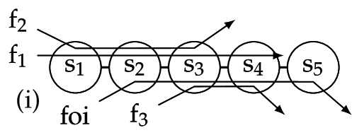
(a) Example tandem network shown in Figure 1

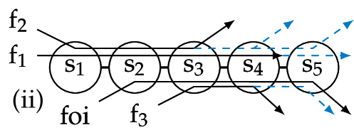
(b) Indication of all its potential flow prolongation alternatives

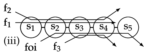
(c) A beneficial prolongation

Figure 2: Sample network with prolongations and a specific FP alternative we will evalaute as an example

Take the sample tandem in Figure 2(a), where bounding the arrivals of data flows $f_{1}$ and $f_{2}$ is required at their first location of interference with the foi, server $s_{2}$. Independent of the FIFO multiplexing assumption, the NC feedforward analysis may suffer from the so-called segregation effect [Bondorf2017a]: both flows assume to only receive service after the respective other flow was forwarded by server $s_{1}$ – an unattainable pessimistic forwarding scenario in the analysis’ internal view on the network. With FP, it is possible to steer the analysis such that it does not have to apply this pessimism. By prolonging flow $f_{2}$ to also cross $s_{4}$, we match its path with $f_{1}$ (see Figure 2(b)) and allow both flows’ output from $s_{1}$ to be bounded in aggregate. Note, that this adds interference to the foi at $s_{4}$ and may therefore not be beneficial for its delay bound after all. Thus, usually all alternative prolongations of flows as shown by the dashed lines in Figure 2(b) must be tested. Although only aiming at improvement (I2), the approach was shown to not scale [Bondorf2017c].

The dominant problem that causes a loss of tightness in the NC FIFO analysis is the lack of the PMOO property, caused by the cuts mentioned in improvement (I1) above. In general, the property is achieved by analyses that first create an end-to-end view on the tandem under analysis. Algebraic FIFO analysis cannot achieve this for non-nested interference patterns (see Section III-C and Figure 2(a), servers $s_{2}$ to $s_{4}$ where cross-flow paths overlap). It can only analyze nested tandems in an end-to-end fashion allowing for full implementation of the PMOO property. FP allows for transforming a non-nested tandem into a nested one. See Figure 2(c) where the path of $f_{2}$ was prolonged over $s_{4}$, causing $f_{3}$ to become nested into $f_{2}$ instead of creating a non-nested interference pattern with it.

Impact Evaluation on Sample Network in Figure 2

As mentioned above and illustrated by Figure 2, the two improvements that can be attained with FP do not necessarily occur in isolation. We provide a detailed evaluation of the impact of the proposed prolongation in our example.

(a) Cutting left of server $s_{3}$

(b) Cutting right of server $s_{3}$

Figure 3: Sample network in Figure 2(a) analyzed with FIFO requires find the best among two possible cut locations

To apply the FIFO analysis to non-nested tandems, such a tandem is cut into a sequence of sub-tandems that all have nested interference patterns only. In Figure 2(a), the tandem can be cut before or after server $s_{3}$ as shown in Figure 3. Either alternative has the very same drawback: a cross-flow is cut, too, depriving the analysis of its end-to-end view on said flow. PMOO is not achieved and bounds become untight.

Let server $s_{i}$ provide service $\beta_{i}$ and let flow $f_{j}$ put $\alpha_{j}$ data into the network. Further denote with $\alpha^{s}$ some arrival curve at server $s$. The respective (min,plus)-algebraic terms bounding the foi’s end-to-end residual service curve are:

$$\beta_{\Theta_{\text{I}},\text{i},\text{left}}\;=\;(((\beta_{3}\ominus_{\theta_{5}}\alpha^{s_{3}}_{2})\otimes\beta_{4})\ominus_{\theta_{6}}(\alpha_{3}+\alpha^{s_{3}}_{1}))$$ (11)

$$\hskip 14.22636pt\otimes(\beta_{2}\ominus_{\theta_{7}}((\alpha_{1}+\alpha_{2})\oslash\beta_{1}))\otimes\beta_{5}$$

$$\text{with}\hskip 14.22636pt\alpha^{s_{3}}_{1} = \alpha_{1}\oslash(((\beta_{2}\ominus_{\theta_{1}}\alpha_{\text{foi}})\otimes\beta_{1})\ominus_{\theta_{2}}\alpha_{2})$$

$$\alpha^{s_{3}}_{2} = \alpha_{2}\oslash(((\beta_{2}\ominus_{\theta_{3}}\alpha_{\text{foi}})\otimes\beta_{1})\ominus_{\theta_{4}}\alpha_{1})$$

for the cut left of $s_{3}$ and $\Theta_{\text{I}}=\{\theta_{1},\ldots,\theta_{7}\}$ and for the cut right to it with $\Theta_{\text{II}}=\{\theta_{8},\ldots,\theta_{16}\}$ to later optimize:

$$\beta_{\Theta_{\text{II}},\text{i},\text{right}}\;=\;(((\beta_{3}\ominus_{\theta_{14}}\alpha_{3})\otimes\beta_{2})\ominus_{\theta_{15}}((\alpha_{1}+\alpha_{2})\oslash\beta_{1}))$$ (12)

$$\hskip 78.24507pt\otimes(\beta_{4}\ominus_{\theta_{16}}\alpha^{s_{4}})\otimes\beta_{5}$$

$$\text{with}\hskip 5.69054pt\alpha^{s_{4}} = (\alpha_{3}+(\alpha_{1}\oslash(((\beta_{2}\ominus_{\theta_{8}}\alpha_{\text{foi}})\otimes\beta_{1})\ominus_{\theta_{9}}\alpha_{2})))$$

$$\hskip 110.96574pt\oslash(\beta_{3}\ominus_{\theta_{10}}\alpha^{s_{3}})$$

$$\alpha^{s_{3}} = ((\alpha_{2}\oslash(\beta_{1}\ominus_{\theta_{11}}\alpha_{1}))+\alpha_{\text{foi}})$$

$$\hskip 51.21495pt\oslash(\beta_{2}\ominus_{\theta_{12}}(\alpha_{1}\oslash(\beta_{1}\ominus_{\theta_{13}}\alpha_{2})))$$

Note, e.g., in $\alpha^{s_{3}}$ the segregation of flows at $s_{1}$ by the simultaneous occurrence of $\alpha_{1}\oslash(\beta_{1}\ominus_{\theta}\alpha_{2})$ and $\alpha_{2}\oslash(\beta_{1}\ominus_{\theta}\alpha_{1})$ in the term that will be used for the right sub-tandem. Moreover note, that the sub-tandem to the left of $s_{3}$ can, in contrast, apply aggregate bounding thanks to flows’ common last server on it. The analysis thus computes $(\alpha_{1}+\alpha_{2})\oslash\beta_{1}$.

With the FP alternative shown in Figure 2(c), neither segregation nor cutting is required and the residual service curve is significantly less complex with $\Theta_{\text{III}}=\{\theta_{a},\theta_{b}\}$:

$$\beta_{\Theta_{\text{III}},\text{iii}}=((((\beta_{3}\otimes\beta_{4})\ominus_{\theta_{a}}\alpha_{3})\otimes\beta_{2})\ominus_{\theta_{b}}((\alpha_{1}+\alpha_{2})\oslash\beta_{1}))\otimes\beta_{5}$$ (13)

We have tested this instantiation of FP for different curve settings and w.r.t. its impact on either bounding the foi delay or output. Service curves were set to $\beta_{R=40,T}$ and arrival curves to $\gamma_{r=u\cdot 10,b}$ where $u$ denotes the utilization $\frac{4r}{R}$ at the server that always sees four flows, $s_{3}$. Latencies $T$ as well as bursts $b$ were set to 0, 0.1 or 10. Note, that our setting guarantees for finite bounds.

For quantification of the improvement, we compute the reduction of the respective bound’s variable part relative to the FIFO bound in the original network. That is, the end-to-end delay bound cannot be decreased below the sum of latencies on the analyzed foi’s path. We incur a fixed latency of $\sum_{i=2}^{5}T_{i}=4T$ in our sample network that we subtract from the bounds computed for the original and the FP network. We call the remaining variable part of the delay bound latency increase $hDevInc$. Its improvement is defined as follows:

$$\frac{\mathit{delay}^{\text{FIFO}}-\mathit{delay}^{\text{FIFO-FP\textsubscript{III}}}}{\mathit{delay}^{\text{FIFO}}}$$

$$=\frac{hDev(\alpha_{\text{foi}},\beta_{\Theta_{\text{I}\wedge\text{II}},\text{i}})-hDev(\alpha_{\text{foi}},\beta_{\Theta_{\text{III}},\text{iii}})}{\mathit{delay}^{\text{FIFO}}}$$

$$=\frac{(hDev(\alpha_{\text{foi}},\beta_{\Theta_{\text{I}\wedge\text{II}},\text{i}})-4T)-(hDev(\alpha_{\text{foi}},\beta_{\Theta_{\text{III}},\text{iii}})-4T)}{\mathit{delay}^{\text{FIFO}}}$$

$$=\frac{hDevInc(\alpha_{\text{foi}},\beta_{\Theta_{\text{I}\wedge\text{II}},\text{i}})-hDevInc(\alpha_{\text{foi}},\beta_{\Theta_{\text{III}},\text{iii}})}{\mathit{delay}^{\text{FIFO}}}$$ (14)

where $hDev(\alpha_{\text{foi}},\beta_{\Theta_{\text{I}\wedge\text{II}},\text{i}})=hDev(\alpha_{\text{foi}},\beta_{\Theta_{\text{I}},\text{i},\text{left}})\wedge hDev(\alpha_{\text{foi}},\beta_{\Theta_{\text{II}},\text{i},\text{right}}).$

We proceed in a similar fashion for quantifying the reduction of the output bound. In our setting with token-bucket arrival curves $\alpha$ and rate-latency service curves $\beta$, the output bound will be a token-bucket arrival curves with its rate equal to the bounded foi’s rate. Thus, we shift our attention to the output bound burstiness $(\alpha\oslash\beta)(0)$ that equals the foi’s end-to-end backlog bound $vDev$ (see Theorem 1). After subtraction of the foi’s inherent burstiness $b_{\text{foi}}=b$, we get the output (bound) burstiness increase $vDevInc$. Its improvement is defined analog to Equation 14 as:

$$\frac{\mathit{output\,burstiness}^{\text{FIFO}}-\mathit{output\,burstiness}^{\text{FIFO-FP\textsubscript{III}}}}{\mathit{output\,burstiness}^{\text{FIFO}}}$$

$$=\frac{(\alpha_{\text{foi}}\oslash\beta_{\Theta_{\text{I}},\text{i},\text{left}})(0)\wedge(\alpha_{\text{foi}}\oslash\beta_{\Theta_{\text{II}},\text{i},\text{left}})(0)}{\mathit{output\,burstiness}^{\text{FIFO}}}$$

$$\hskip 113.81102pt-\hskip 5.69054pt\frac{(\alpha_{\text{foi}}\oslash\beta_{\Theta_{\text{III}},\text{iii}})(0)}{\mathit{output\,burstiness}^{\text{FIFO}}}$$

$$=\frac{(vDev(\alpha_{\text{foi}},\beta_{\Theta_{\text{I}\wedge\text{II}},\text{i}})-b)-(vDev(\alpha_{\text{foi}},\beta_{\Theta_{\text{III}},\text{iii}})-b)}{\mathit{output\,burstiness}^{\text{FIFO}}}$$

$$=\frac{vDevInc(\alpha_{\text{foi}},\beta_{\Theta_{\text{I}\wedge\text{II}},\text{i}})-vDevInc(\alpha_{\text{foi}},\beta_{\Theta_{\text{III}},\text{iii}})}{\mathit{output\,burstiness}^{\text{FIFO}}}$$ (15)

where $vDev(\alpha_{\text{foi}},\beta_{\Theta_{\text{I}\wedge\text{II}},\text{i}})=vDev(\alpha_{\text{foi}},\beta_{\Theta_{\text{I}},\text{i},\text{left}})\wedge vDev(\alpha_{\text{foi}},\beta_{\Theta_{\text{II}},\text{i},\text{right}})$.

Figure 4 shows the results of evaluating these two improvements by FP, subject to increasing peak utilization on the foi’s path. For both metrics, we achieve a considerable improvement already for lowest utilizations as well as $T=0$ and $b=0$, respectively. These results motivate our work on integrating FP into the feedforward analysis.

Notably, the delay bound improvement is influenced by the peak utilization by a far larger extent as shown in Figure 4(a). For $T=10$, we even observe a decrease of improvement. An important impact factor is again the lack of the PMOO property. In both residual service curves, $\beta_{\Theta_{\text{I}},\text{i},\text{left}}$ and $\beta_{\Theta_{\text{II}},\text{i},\text{right}}$, cutting causes the need to compute the output bound of the first subtandem, see occurrences of the deconvolution $\oslash$ in both terms. If the operation takes a residual service curve, not only the latency $T$ is considered but also yet another latency increase. This increase is grows with the peak utilization, not leading to a linear increase of the improvement. We leave a thorough investigation for future work.

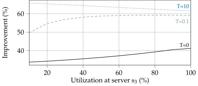
(a) Delay bound improvements

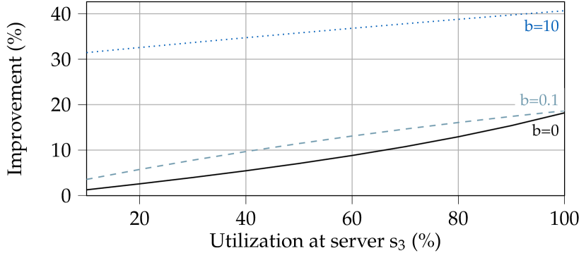
(b) Output bound burstiness improvement

Figure 4: Improvements of the foi’s delay bound and output bound burstiness by applying FP alternative Figure 2(c) in the NC FIFO analysis of the network in Figure 2(a)

IV-B The Challenge to Apply FP

The study of NC analysis scalability demands appropriate tool support. For the analysis of feedforward networks, we extended the implementation provided by the NCorgDNC v2.7 [Bondorf2014, Scheffler2021]. Previous work [GeyerSchefflerBondorf_RTAS2021] used the tool provided by Bisti et al. [Bisti2008, Bisti2012] that is limited to the study of tandem networks. Additionally, we benchmark against the FFMILPA and FFLPA [Bouillard2015] by using another tool. A recent overview on further NC tools can be found in [Zhou2020].

Analysis Scalability

As mentioned in Section I and illustrated in Figures 1(a) and 2, on each tandem with $n$ hops and $m$ cross-flows, FP may explore $O(n^{m})$ prolongation alternatives. This raises doubts about its general scalability, confirmed in [Bondorf2017c]. Moreover, FFMILPA is known to not scale well either. Its heuristic FFLPA is assumed to neither do so [Bouillard2022]. Therefore, we ran all analyses on a sample dataset of networks with up to 500 flows (see Section V-C), setting a time limit of $1\text{\,}\mathrm{h}$ and a memory limit of $5\text{\,}\mathrm{G}\mathrm{B}$ for each flow analysis.

Results are presented in Figure 5. FIFO-FP, the exhaustive search for the best FP alternative on all tandems, was able to terminate for only $28\text{\,}\mathrm{\char 37\relax}$ of flows. The successful termination ratio is roughly equal for FFMILPA. However, as both analyses are fundamentally different, their sets of analyzed flows are only equal for about $57.5\text{\,}\mathrm{\char 37\relax}$.

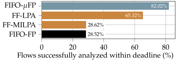
Figure 5: Flows successfully analyzed with a $1\text{\,}\mathrm{h}$ deadline and at most $5\text{\,}\mathrm{G}\mathrm{B}$ memory usage

FP’s Explored Alternatives

The sheer amount of possible prolongation alternatives is the very cause of FIFO-FP’s limited scalability. In an attempt to scale FIFO-FP to analyze a larger set of flows, we created a heuristic that ignores certain alternatives. We base this heuristic, called FIFO-$\mu$FP, on [Bondorf2017c] where the analysis paired with FP does not suffer from cutting and thus improvement (I2) from above was evaluated in isolation. It did not show significant potential. In FIFO-$\mu$FP, we therefore restrict the search for a beneficial FP alternative to check for improvement (I1). We do so by checking for non-nested interference patterns and prolonging all involved flows to match the path of the longest flow. FIFO-$\mu$FP may create new non-nested patterns by a prolongation, yet, we do not check any further. Figure 5 already shows the amount of analyzed flows at $82\text{\,}\mathrm{\char 37\relax}$ highest among all analyses.

Still, the amount of prolongation alternatives for the dataset evaluated in this article is forbiddingly large, see Figure 6. Note for a large number of cross-flows, networks may have been excluded from this preliminary evaluation due to the limits set for computing data. As expected, we get an exponential scaling between the number of cross-flows and the number of explored alternatives.

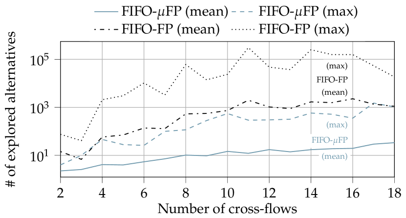
Figure 6: Relation between the number of cross-flows and the explored FP alternatives by FIFO-$\mu$FP and FIFO-FP

Last, to allow further fine-tuning of the tradeoff between delay bound tightness and computational effort, we may set the number of explored FP alternatives to a fixed $k$ in our analyses. E.g., we will evaluate the performance of DeepFP_k for some values $k\geq 1$ in Section VI.

V Effective FP Predictions with GNN

We develop our universal DeepFP heuristic in this section, based in part on the work proposed in DeepTMA [Geyer2019a, Geyer2020]. As illustrated in Figure 1, the main intuition behind DeepFP is to avoid the exhaustive search for the best prolongation by limiting it to a few alternatives. The heuristic’s task is then only to predict the best flow prolongations, which are then fed to the NC analysis. This ensures that the bounds provided are formally valid.

For DeepFP, we used a GNN as heuristic, since it was shown in DeepTMA to be a fast and efficient method [Geyer2019a, Geyer2020b]. We define networks to be in the NC modeling domain and to consist of servers, crossed by flows. We refer to the model used in GNN as graphs. During the different steps of the NC FIFO analysis, the sub-networks of interest are passed to the GNN by transforming the networks into graphs (see Section V-B) and processing them with the GNN. The outputs of the GNN are then fed back to the NC analysis, which finally performs its (min,plus) computations using the prolongations suggested by the GNN.

V-A GNN Fundamentals

We use the framework of GNN introduced in [Gori2005, Scarselli2009]. They are a special class of NN for processing graphs and predict values for nodes or edges depending on the connections between nodes and their properties. The idea behind GNN is called message passing, where so-called messages, i.e., vectors of numbers $\mathbf{h}_{v}\in\mathbb{R}^{k}$, are iteratively updated and passed between neighboring nodes. Those messages are propagated throughout the graph using multiple iterations until a fixed point is found or until a fixed number of iterations. We refer to [Gilmer2017] for a formalization of many concepts recently developed around GNN.

Each node in the graph $v$ has input features, e.g., server rate, flow burstiness, labeled $\mathbf{i}_{v}$, and output features, e.g., prolongation choices, labeled $\mathbf{o}_{v}$. Specific input and output features used for DeepFP will be explained in Section V-B.

The final messages are then used for predicting properties about nodes, namely the flow prolongations in our case. This concept can be formalized as:

$$\mathbf{h}_{v}^{(t)} =\mathit{aggr}\left(\left\{\mathbf{h}_{u}^{(t-1)}\;\middle|\;u\in\textsc{Nbr}(v)\right\}\right)$$ (16)

$$\mathbf{o}_{v} =\mathit{out}\left(\mathbf{h}_{v}^{(t\to\infty)}\right)$$ (17)

$$\mathbf{h}_{v}^{(t=0)} =\mathit{init}\left(\mathbf{i}_{v}\right)$$ (18)

with $\mathbf{h}_{v}^{(t)}$ representing the message from node $v$ at iteration $t$, $\mathit{aggr}$ a function which aggregates the set of messages of the neighboring nodes $\textsc{Nbr}(v)$ of $v$, $\mathit{out}$ a function transforming the final messages to the target values, and $\mathit{init}$ a function for initializing the messages based on the nodes’ input features.

Various approaches to GNNs have been recently proposed in the literature, mainly reusing the message passing framework from Equations 16 to 19 with different implementations for the $\mathit{aggr}$ and $\mathit{out}$ functions. We selected GGNN [Li2016a] for our GNN model, with the addition of edge attention. For each node $v$ in the graph, its message $\mathbf{h}_{v}^{(t)}$ at iteration $t$ is updated at each iteration as:

$$\mathbf{h}_{v}^{(t=0)} =\mathit{FFNN}_{\mathit{init}}\left(\mathbf{\mathit{inputs}}_{v}\right)$$ (19)

$$\mathbf{h}_{v}^{(t)} =\mathit{GRU}\left(\mathbf{h}_{v}^{(t-1)},\sum_{u\in\textsc{Nbr}(v)}\lambda_{(u,v)}^{(t-1)}\mathbf{h}_{u}^{(t-1)}\right)$$ (20)

$$\lambda_{(u,v)}^{(t)} =\sigma\left(\mathit{FFNN}_{\mathit{edge}}\left(\left\{\mathbf{h}_{u}^{(t)},\mathbf{h}_{v}^{(t)}\right\}\right)\right)$$ (21)

$$\mathit{outputs} =\mathit{FFNN}_{\mathit{out}}(\mathbf{h}_{v}^{(d)})$$ (22)

with $\sigma(x)=1/(1+e^{-x})$ the sigmoid function, $\textsc{Nbr}(v)$ the set of neighbors of node $v$, $\{\cdot,\cdot\}$ the concatenation operator, $\mathit{GRU}$ a GRU cell, $\mathit{FFNN}_{\mathit{init}}$, $\mathit{FFNN}_{\mathit{edge}}$, $\mathit{FFNN}_{\mathit{out}}$ three FFNN, and $\lambda_{(u,v)}\in(0,1)$ the weight for $(u,v)$. The final prediction for each node is performed using FFNN (see Equation 22) after applying Equation 20 for $d$ iterations, with $d$ corresponding to the diameter of the analyzed graph.

V-B Model Transformation

Since we work with ML method, we need an efficient data structure for describing NC network which can be processed by NN. We chose undirected graphs, as they are a natural structure for describing networks and flows. Due to their varying sizes, networks of any sizes may be analyzed using our method.

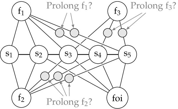
Figure 7: Graph encoding of the network from Figure 2(a)

We only use the servers and flows relevant to the current foi for the graph transformation by recursively backtracking through the server graph based on the foi’s path. We name this sub-network as sub-network of interest $\mathcal{N}_{\text{foi}}$. We follow Algorithm 1 for this graph transformation, also illustrated and applied in Figure 7 on the network from Figure 2(a). Each server is represented as a node in the graph, with edges corresponding to the network’s links. The features of a server node are its service curve parameters, namely its rate and latency, and its order w.r.t the foi’s path. Each flow is represented as a node in the graph, too. The features of a flow node are its arrival curve parameters, namely its rate and burst in case of a token-bucket arrival curve. Additionally, the foi receives an extra feature representing the fact that it is the analyzed flow.

Algorithm 1 Graph transformation of network $\mathcal{N}_{\text{foi}}$

$\mathcal{G}:=$ empty undirected graph

for all server $s_{i}$ in network $\mathcal{N}_{\text{foi}}$ do $\mathcal{G}$.addNode($s_{i}$)

for all link $(s_{i},s_{j})$ in network $\mathcal{N}_{\text{foi}}$ do $\mathcal{G}$.addEdge($s_{i}$, $s_{j}$)

for all flow $f_{i}$ in network $\mathcal{N}_{\text{foi}}$ do

     $\mathcal{G}$.addNode($f_{i}$)

     for all server $s_{j}$ in $f_{i}$.path() do $\mathcal{G}$.addEdge($f_{i}$, $s_{j}$)

for all flow $f_{i}$ in network $\mathcal{N}_{\text{foi}}$ excluding foi do

     for all server $s_{j}$ in foi’s path do

         if prolongation $P_{f_{i}}^{s_{j}}$ of flow $f_{i}$ to $s_{j}$ is valid then

              $\mathcal{G}$.addNode($P_{f_{i}}^{s_{j}}$)

              $\mathcal{G}$.addEdges((${f_{i}}$, $P_{f_{i}}^{s_{j}}$), ($P_{f_{i}}^{s_{j}}$, $s_{j}$))               return $\mathcal{G}$

To encode the path taken by a flow in this graph, we use edges to connect the flow to the servers it traverses. Compared to the original DeepTMA graph model from [Geyer2019a], we simplify one aspect: we do not include path ordering nodes that tell us the order of servers on a crossed tandem. The ordering is represented by the server order feature, which is the distance relative to the foi’s sink.

To represent the flow prolongations, prolongation nodes ($P_{f_{i}}^{s_{j}}$) connecting the cross-flows to their potential prolongation sinks are added to the graph. Those nodes contain the hop count according to the foi’s path as main feature – this is sufficient to later feed the prolongation into the NC analysis, path ordering nodes are not required for this step either. A prolongation node is also used for the last server of a cross-flow’s unprolonged path (e.g. $s_{4}$ for $f_{1}$ in Figure 7). Those nodes represent the choice to not prolong a given flow.

Based on this graph representation, the task of the GNN is to predict prolongation for each cross-flow by choosing the last server to prolong to. Namely for each cross-flow $f$ and each potential sink $s$, the NN assigns a probability value $\Pr_{f,s}$ between 0 and 1 to the corresponding prolongation node. For each flow, the prolongation node with the highest probability decides which sink to use for prolonging the flow. As illustrated in Figure 1(b), those predictions are then fed to FIFO-FP, which finally performs the NC analysis.

V-C Implementation

We implemented the GNN used in DeepFP using PyTorch [Paszke2019b] and PyG [Fey2019]. Optimal parameters for the NN size and the training were found using hyper-parameter optimization. Table I illustrates the size of the GNN used for the evaluation in Section VI.

Table I: Size of the GNN used in Section VI. Indexes represent respectively the weights ($w$) and biases ($b$) matrices

Layer	Size of the weights and bias matrices
$\mathit{FFNN}_{\mathit{init}}$	$(13,128)_{w}+(128)_{b}$
Message passing	$(128,128)_{w}+2\times\left\{(384,128)_{w}+(128)_{b}\right\}$
$\mathit{FFNN}_{\mathit{edge}}$	$\left\{(256,128)_{w}+(128)_{b}\right\}+\left\{(128,1)_{w}+(1)_{b}\right\}$
$\mathit{FFNN}_{\mathit{out}}$	$\left\{(128,128)_{w}+(128)_{b}\right\}+\left\{(128,1)_{w}+(1)_{b}\right\}$
Total:	$166\,402$ parameters

The GNN and the NC analysis are split into two processes during training, as shown in Figure 8. During evaluation, we integrated the graph transformation and the GNN in NCorgDNC using PyTorch’s Java bindings, thus avoiding any inter-process communications.

V-D Dataset Generation

To train and evaluate our NN architecture, we generated a set of random topologies (as to check the FP preconditions of Section IV) according to three different random topology generators: a) tandems, b) trees and c) random server graphs following the $G(n,p)$ Erdős-Rényi model [Erdos1959]. For each created server, a rate-latency service curve was generated with uniformly random rate and latency parameters. A random number of flows was generated with random source and sink servers. Note that in our topologies, there cannot be cyclic dependency between the flows. For each flow, a token-bucket arrival curve was generated with uniformly random burst and rate parameters. All curve parameters were normalized to the $(0,1]$ interval.

For each generated network, the NCorgDNC v2.7 [Bondorf2014] is then used for analyzing each flow. We extended the feedforward LUDB analysis of [Scheffler2021] by the FP feature to implement FIFO-FP, FIFO-$\mu$FP as well as DeepFP. Each analysis is run with a maximum deadline of $1\text{\,}\mathrm{h}\mathrm{o}\mathrm{u}\mathrm{r}$ and maximum RAM usage of $5\text{\,}\mathrm{G}\mathrm{B}$.

Since FIFO-FP may not bring any benefits compared to FIFO, either due to no alternatives for prolonging flows or no end-to-end delay improvement by any alternative, we restrict the dataset to networks and flows where FP is applicable, i.e., flows with prolongation options. Table II contains statistics about the generated dataset. In total approximately $50\,000$ flows were generated and evaluated for the training dataset, and $20\,000$ for the numerical evaluation presented in Section VI. The evaluation dataset is split into two parts: small networks with up to 40 flows as in the training set, and larger networks with 100 to 493 flows. The dataset will be available online to reproduce our results.

Table II: Statistics about the generated dataset

Dataset	Train			Evaluation
Parameter	Min	Mean	Max	Min	Mean	Max
# of servers	5	10.0	15	5	11.2	30
# of flows	12	32.0	40	5	192.1	493
Flow path len	3	4.0	6	3	4.6	14
# of cross-flows	6	20.7	31	2	132.4	492

V-E NN Training

We use RL approach [Sutton2018] for training the GNN, where the optimal solution, i.e., the optimal flow prolongations, is not required to be known for training the GNN. This is different from previous works applying GNN to NC [Geyer2019a, Geyer2020b, GeyerSchefflerBondorf_RTAS2021] where SL was used, i.e., where the best solution was known by running the exhaustive FP analysis.

V-E1 RL

Our RL approach is illustrated in Figure 8. The GNN interacts with the NC FIFO analysis by providing it with flow prolongations. As a feedback, the GNN receives the end-to-end delay or output bound corresponding to the provided flow prolongations. This bound is used for computing the reward, defined as the relative bound improvement over the standard FIFO analysis without prolongations:

$$\mathit{reward}=\frac{\mathit{bound}_{\text{FIFO}}-\mathit{bound}_{\text{FP}}}{\mathit{bound}_{\text{FIFO}}}$$ (23)

The GNN is trained to maximize the reward, i.e., produce prolongations leading to the best improvements over the standard FIFO analysis. Prolongations leading to a worse bound will result in a negative reward.

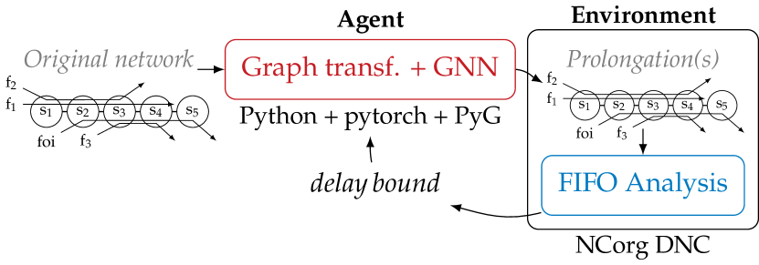
Figure 8: GNN training using the RL approach

As opposed to more advanced applications of RL where a series of actions are required, the agent produces here only a single action, i.e., the GNN produces a single set of flow prolongations to apply to a given network and its flow(s) of interest. Hence, we use here the REINFORCE algorithm [Williams1992], a policy gradient RL approach. The agent’s decision making procedure is characterized by a policy $\pi(a,s,\omega)=\Pr(a|s,\omega)$, with $a$ the actions, i.e., flow prolongations, $s$ the state, i.e., the server graph, and $\omega$ the parameters of the policy, i.e., the weights of the GNN. The policy $\pi$ is defined as a categorical distribution for each flow, where the categories correspond to the different servers with the potential for prolongation.

At each training iteration, the actions $a$ are randomly sampled from the policy $\pi$ and passed to the NC FIFO analysis. As feedback, the resulting delay bound from the NC analysis is received and the reward is calculated according to Equation 23. The parameters of the policy $\pi$ are then updated as:

$$\omega\leftarrow\omega-\nabla_{\omega}\log\pi(a,s,\omega)\cdot\mathit{reward}$$ (24)

To improve the training of the RL policy, we used three well-known approaches. First, we use an $\epsilon$-greedy exploration strategy where the action is either randomly sampled from the current policy with probability $1-\epsilon$, or randomly sampled from a uniform distribution with probability $\epsilon$. Secondly, we use UREX [Nachum2017] to encourage undirected exploration of the reward landscape. This adds a factor in Equation 24 which promotes actions with low probability from the current policy but high reward. Our numerical evaluations showed that UREX performed better than standard entropy regularization commonly used with REINFORCE. Thus, we only use UREX in the following. Finally, we also use curriculum learning, where we gradually increase the difficulty of the prolongation task, numerically defined here as the product between the foi’s path length and the number of cross-flows which can be prolonged.

V-E2 SL

Our main motivation for using RL is that SL would require to extensively run the NC FIFO analysis on the training dataset for getting the optimal prolongations. The computational cost of this task was already illustrated by the small percentage of analyses that finish within the execution time and memory restrictions (Figure 5). To evaluate the impact of a limited dataset in SL as compared to RL, we also trained the GNN using SL approach. We follow the method explained in Section V-E1, with action $a$ being inferred from the result of FIFO-FP or FIFO-$\mu$FP instead of sampling the policy $\pi$ for a random action. We illustrate the impact of SL on the bounds quality in Section VI-A1.

V-E3 Training for Output Bounding

Setting the free $\theta$ parameters in the NC FIFO analysis’ residual service curve term can vastly differ between bounding delay and output. Since FP is used when bounding the output of flows, too, we also query the GNN for predicting prolongations under this objective. We specifically trained a version of DeepFP where the NC FIFO analysis computes the output bound as the $\mathit{reward}$. A numerical evaluation showed no significant gains using this additional effort compared to training solely on the prolongations for delay bounding. I.e., the cuts removed by FP for best improvement of the delay bound are with very few exceptions also those to be removed for improving the output bound. Hence, we restrict to training GNN with the delay bound as $\mathit{reward}$.

V-E4 From Add-on Feature to Full Analysis

As noted in Section III-D, FP was originally designed as an add-on feature for NC analyses. Our preliminary investigation using SL [GeyerSchefflerBondorf_RTAS2021] showed promising results such that we diverge from this previous view in our FIFO analysis. We promote DeepFP to a full analysis, meaning we only evaluate the $k$-predicted FP alternatives. Note, that the original paths might be predicted, too, and that any predicted prolongation will give a valid delay bound (see Section III-D).

VI Numerical Evaluation

Our numerical evaluation aims to answer two questions:

1. How much delay bound improvement can FP achieve?

2. How do the analyses scale?

In order to illustrate the benefits of DeepFP, we also provide comparisons against two analyses that select prolongation alternatives at random:

1. RND_$k$ selects from all possible FP alternatives

2. $\mu$RND_$k$ adds some expert knowledge to select only from the FP alternatives that are explored by FIFO-$\mu$FP

As before, $k$ denotes the number evaluated alternatives such that $k\geq 1$. We may omit $k$ if $k=1$.

In the following, we show details about DeepFP performance in terms of tightness as well as execution time. Improvements in both will directly be applicable to and have an impact on any real-world application of the NC methodology. All evaluations presented here were done with the evaluation dataset described in Section V-D. Each analysis was limited to $1\text{\,}\mathrm{h}$ execution time and $5\text{\,}\mathrm{G}\mathrm{B}$ memory.

VI-A Delay Bound Improvements

We compare in this section the gain in tightness for the delay bound compared against FIFO. To evaluate this gain, we use the delay bound gap metric for showing its increase:

$$\mathit{delay\,bound\,gap}_{\text{foi}}=\frac{delay_{\text{foi}}^{\text{FIFO}}-delay_{\text{foi}}^{\text{method}}}{delay_{\text{foi}}^{\text{FIFO}}}$$ (25)

VI-A1 RL vs. SL

Previous works applying GNN to NC [Geyer2019a, Geyer2020b, GeyerSchefflerBondorf_RTAS2021] used SL-based approach. For a comparison to SL, we ran FIFO-FP and FIFO-$\mu$FP on the fraction of our training dataset that finished analyzing under the time and memory restrictions (see Section IV-B). While FIFO-$\mu$FP yields inferior prolongations, it creates a larger dataset to learn from than FIFO-FP does. Prolongations from both analyses were then used as target for training two separate GNN. The RL-approach for training the GNN was implemented as described in Section V-E.

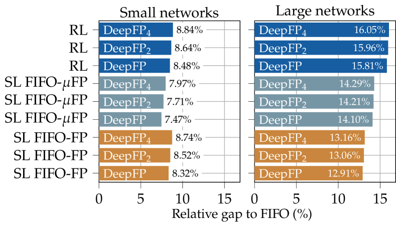
Figure 9: Impact of RL vs. SL on the average bound gap

On smaller networks, we notice that the predictions of the GNN produce similar relative gaps when trained with RL or SL with FIFO-FP, with a small advantage for RL. On larger networks, RL has a clear edge over SL, stemming from two facts: a) the training data for SL could only be generated on a subset of the smaller networks and b) RL can explore the aggregation potential of FP (see Section IV-A). This is further illustrated on the GNN trained with SL on FIFO-$\mu$FP, which achieves better delay bounds, yet still fails due to prolongations of lower quality than FIFO-FP.

Overall this illustrates that knowing the best prolongations is not necessarily required for training the GNN. Using a pure RL approach without manually created training data can actually yield better results.

VI-A2 RL performance

In the following, we restrict our depiction on DeepFP using the RL-trained GNN. As shown in Section IV-B, competing analyses were not necessarily able to analyze the entire evaluation dataset due to their poor scalability. We restrict the following comparisons to those flows, across all considered networks, where the computation of the delay bound finished within $1\text{\,}\mathrm{h}$ with maximally $5\text{\,}\mathrm{G}\mathrm{B}$ memory usage. We present our results on increasing evaluation datasets.

First, we compare DeepFP against the tight FFMILPA and its heuristic FFLPA on the flows that all analyses were able to analyze. Figure 10 shows that FFMILPA tightens delay bounds more than FIFO-FP and thus DeepFP. However, this comes at a much greater computational cost as we show in LABEL:sec:execution_time. Overall, DeepFP and FIFO-FP perform well and exploring multiple prolongation alternatives yields larger improvements yet these are only marginally better.

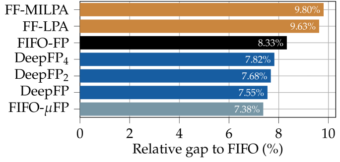
Figure 10: Average delay bound gap on the subset of flows successfully analyzed with FFMILPA, FFLPA and FIFO-FP

An evaluation of the similarly large dataset that FIFO-FP was able to analyze with its naïve bruteforce approach is shown in Figure 11. It illustrates how well DeepFP performs compared to the best prolongations. DeepFP computes on average similarly improved delay bounds as before, close to FIFO-FP. Notably, on this dataset it beats the FIFO-$\mu$FP heuristic based on previous insights (see Section IV-B). Thus, it also beats $\mu$RND_$k$, even with fewer explored prolongation alternatives. RND_$k$ is less competitive than $\mu$RND_$k$, as expected due to it selecting FP alternatives from a larger pool that covers more potentially bad ones.

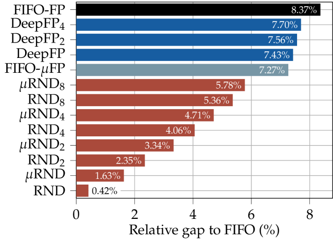
Figure 11: Average delay bound gap on the subset of flows successfully analyzed with FIFO-FP and FIFO-$\mu$FP

Further increasing the dataset, we next compare DeepFP against FIFO-$\mu$FP in LABEL:fig:reldelay_nofp_subset_heuristicffp. We partition networks into small and large to better visualize trends. On the small networks, DeepFP’s average delay bound gap is comparable with the one of FIFO-$\mu$FP but does not exceed it anymore. The gap to FIFO-$\mu$FP increases on the large networks, indicating that DeepFP has some difficulties to generalize.

Moreover, the larger the networks become, the better $\mu$RND_$k$ seems to perform against RND_$k$. In the small networks in LABEL:fig:reldelay_nofp_subset_heuristicffp, we see a simple ranking by increasing $k$: RND_$k$ is outperformed by $\mu$RND_$k$ that, in turn, is outperformed by RND_$k+1$. In the larger networks, however, $\mu$RND alreadyperformsaswellasRND_$4$andμRND_$2$alreadyoutperformsRN