Dark Matter in Galaxy Clusters:
a Parametric Strong Lensing Approach

We present a parametric strong lensing analysis of three massive galaxy clusters for which Hubble Space Telescope imaging is available, as well as spectroscopy of multiply imaged systems and galaxy cluster members.

Our aim is to probe the inner shape of dark matter haloes, in particular the existence of a core.

We adopt the following working hypothesis: any group/cluster scale dark matter clump introduced in the modelling should be associated with a luminous counterpart. We also adopt some additional well motivated priors in the analysis, even if this degrades the quality of the fit, quantified using the RMS between the observed and model generated images.

In particular, in order to alleviate the degeneracy between the smooth underlying component and the galaxy scale perturbers, we use the results from spectroscopic campaigns by Bergamini et al. (2019) allowing to fix the mass of the galaxy scale component.

In the unimodal galaxy cluster AS 1063, a cored mass model is favored with respect to a non cored mass model, and this is also the case in the multimodal cluster MACS J0416. In the unimodal cluster MACS J1206, we fail to reproduce the strong lensing constraints using a parametric approach within the adopted working hypothesis. We then successfully add a mild perturbation in the form of a superposition of B-spline potentials which allows to get a decent fit (RMS = 0.5$\arcsec$), finally finding that a cored mass model is favored. Overall, our analysis suggest evidence for cored cluster scale dark matter haloes in these three clusters. These findings may be useful to interpret within alternative dark matter scenario, as self interacting dark matter.

We propose a working hypothesis for parametric strong lensing modelling where the quest for the best fit model will be balanced by the quest for presenting a physically motivated mass model, in particular by imposing priors.

1 Introduction

Dark Matter (DM) is an elusive component which is supposed to largely dominate the mass budget in astrophysical objects over a wide range of scales, in particular in galaxy clusters. However, more than 80 years after the first indirect evidence for DM in galaxy clusters (Zwicky 1937), we have no definitive clues about its existence even though it is sometimes taken for granted. Indeed, evidence for DM are indirect only and no well understood and characterized particle detector has detected it yet, despite intense works amongst the community (see, e.g., Irastorza & Redondo, 2018; Schumann, 2019). As long as such a direct detection has not been reliably achieved, DM remains an hypothesis.

In this paper, we assume the DM hypothesis and we focus on its distribution on cluster scales, using parametric strong lensing techniques. Indeed, strong lensing (SL) is an essential probe of the DM distribution in the centre of galaxy clusters, where the mass density is so high that space time is locally deformed such that multiple images of background sources can form, providing valuable constraints on the mass distribution.

Parametric SL mass modelling relies on the following working hypothesis, supported by N-body simulations: a galaxy cluster is an object composed of different mass clumps, each component being associated with a luminous counterpart and which can (to some extent) be described parametrically. One advantage of parametric SL modelling is that the description of these mass clumps can be directly compared with theoretical expectations. However, a parametric description is sometimes not accurate nor adapted, emphasizing the limit of parametric mass modelling and the need for more flexible approaches.

We usually have two types of mass clumps: cluster scale DM clumps (whose typical projected mass within a 50$\arcsec$ aperture is of order 10¹⁴M_☉ at $z\sim$ 0.2) and galaxy scale DM clumps associated with individual galaxies. Added to that description of the dominant DM component, one can also consider in the modelling mass components associated with the X-ray gas (Paraficz et al., 2016; Bonamigo et al., 2018).

Parametric SL modelling displays interesting and puzzling features.

Let us mention two of them that will be addressed in this paper. First, it sometimes requires DM clumps whose position do not coincide with any luminous counterpart. This is the case in complicated merging clusters, for example MACS J0717 (Limousin et al., 2016) or Abell 370 (Lagattuta et al., 2019), where parametric mass modelling might not be the best modelling method. This also happens in apparently unimodal clusters (e.g. MACS J1206 studied in this work). These ”dark” clumps are usually added in order to improve significantly the fit but the physical interpretation of these clumps is not straightforward and, taken for granted, their inclusion in the mass budget might be misleading: ”are we really witnessing a dark clump?”. These ”dark” clumps are more likely to express the limitations of parametric mass modelling in some clusters. In this case, the advantage of parametric mass modelling mentioned above might lose their relevance.

Second, large core radii (sometimes larger than 100 kpc) are sometimes reported in parametric SL studies (e.g. Sand et al., 2004; Richard et al., 2010; Newman et al., 2013; Lagattuta et al., 2019; Richard et al., 2021), which have some implications for cosmological models (see discussion by Limousin et al., 2016, L16 hereafter.).

Finally, some mass models do require non negligible external shear component ($\gamma_{\rm ext}$) in order to significantly improve the goodness of the reconstruction, but the physical origin of this external shear is not always clear, for example in Abell 370 ($\gamma_{\rm ext}$=0.13, Lagattuta et al., 2019), in MACS J0329 and RX J1347 ($\gamma_{\rm ext}$=0.07 and 0.10 respectively, Caminha et al., 2019), in MACS J1206 ($\gamma_{\rm ext}$=0.12, Bergamini et al., 2019), in Abell 2744 ($\gamma_{\rm ext}$=0.17, Mahler et al., 2017) and in SDSS 1029 ($\gamma_{\rm ext}$=0.09, Acebron et al., 2022). This component can have either a physical origin or might be compensating for the limitations of the parametric modelling. In practice, the origin of this external shear can be missed since it can be due to substructures located far from the cluster core (Acebron et al., 2017) in regions not covered in narrowly targeted observations as the one carried out with the HST.

Interestingly enough, some alternatives to the current cosmological $\Lambda$ Cold Dark Matter ($\Lambda$CDM) scenario allow for the formation of cores and offsets between luminous and dark components at galaxy cluster scale, as self interacting dark matter (SIDM) models. For a recent review on the SIDM alternative, see Tulin & Yu (2018).

A thorough SIDM investigation of the size of the core radii in the galaxy cluster mass regime is still lacking, but we have some hints about its order of magnitude. With low statistics (50 haloes resolved), Rocha et al. (2013) do quantify haloes core sizes in SIDM simulations with a cross section equal to 1 cm²/g to be in the range 55-90 kpc. Their simulations with a cross section equal to 0.1 cm²/g are not resolved enough to measure a core radius, but they predict core radii to be in the range 10-12 kpc. Robertson et al. (2017) report core radii smaller than 40 kpc. Such an upper bound is also found when self interaction is ”frequent” instead of ”rare” (Fischer et al., 2021).

Regarding offsets between stellar and DM components in the SIDM scenario, studies have shown that such offsets should be small. In the case of the merging Bullet Cluster where DM clumps positions are well constrained by SL, no such offsets has been detected, providing an upper limit on the self interacting cross section of DM equal to 1.25 cm²/g (Randall 2008).

According to simulations by Kim et al. (2017), in merging clusters, a maximal galaxy DM offset of 20 kpc forms for a self interaction equal to 1 cm²/g. They also find that the maximal one before completely disrupting the haloes is $\sim$100 kpc in an ideal case. Robertson et al. (2017), presenting SIDM simulations with anisotropic scattering, report DM-galaxy offsets smaller than 10 kpc. Fischer et al. (2021), in simulations of SIDM equal mass mergers with frequent self interactions, claim that frequent self interactions can cause much larger offsets than rare self interactions. These offsets do vary with time and are non zero after the first pericentre passage. For a self interaction of 1.0 cm²/g they are found to be smaller than $\sim$ 100 kpc (versus 50 kpc for rare self interactions of the same strength). Harvey et al. (2019) investigated the median BCG offset for different dark matter cross sections using the BAryons and HAloes of MAssive Systems simulations (BAHAMAS, McCarthy et al., 2016) and found the median offset to be below 10 kpc.

To conclude, within an SIDM scenario, core radii should be smaller than $\sim$ 100 kpc. Besides, any offset between stellar and DM components should be smaller than $\sim$ 100 kpc.

The main aim of this paper is to investigate the shape of DM at the galaxy cluster scale, in particular its central shape and the eventual presence of a core, following the work presented by L16.

Constraints on DM properties, in particular its central shape, derived from SL have been hampered by the degeneracies inherent to this technique. Strong lensing being sensitive to the total projected mass, it can sometimes be difficult to get insights into the underlying central DM distribution, suggesting the need for robust and well motivated priors in order to break these degeneracies.

One of the main degeneracy is the one between the smooth and the galaxy scale DM components. L16 have shown that, even in the Hubble Frontier Fields era where up to hundreds of multiple images can be detected, this degeneracy still exists and prevents us from getting insights on the DM distribution, in particular on its central shape and the presence of a core.

A promising avenue is to use priors on the galaxy scale perturbers. Recent work by Bergamini et al. (2019, B19 hereafter) propose to use kinematics of cluster members in order to alleviate this degeneracy by providing well motivated priors on the mass of galaxy scale perturbers that are used in the SL mass modelling.

In this paper, we revisit the mass models of three clusters for which B19 have derived reliable constraints on the galaxy scale perturbers to be used as priors in the SL modelling. Our main aim is to investigate whether including these priors can effectively break the above mentioned degeneracy and help in providing constraints on the inner shape of the underlying DM distribution. More precisely, following L16, we aim to see if we can disentangle between a cored and a non cored mass model.

Other priors will also be considered, which are aimed at presenting physically motivated mass models. In particular we impose light and mass to coincide within a few arcseconds. At the redshift of the clusters considered in this work, this translates into a few dozen of kpc, i.e. of the order of what is allowed by SIDM scenarios.

We will see that imposing priors sometimes leads to decreasing the quality of the SL fit. This leads to the following relevant (open) question: ”What is the balance between improving the fit and presenting a mass model which is physically relevant and reliable?” This work also aims at providing some hints about this question.

2 Methodology

2.1 dPIE profile

Dark matter mass clumps are described using a dual Pseudo Isothermal Elliptical Mass Distribution (dPIE profile). We refer the reader to Limousin et al. (2005) and Elíasdóttir et al. (2007) for a description of this mass profile. Here we give a brief overview. It is parametrised by a fiducial velocity dispersion $\sigma$, a core radius $r_{\rm{core}}$ and a scale radius $r_{s}$, sometimes referred to as cut radius in other publications using this profile. We prefer using $r_{s}$ instead of $r_{\rm cut}$. Indeed, it can be shown that this scale radius corresponds to the radius containing half the 3D mass (Elíasdóttir et al., 2007), hence $r_{\rm cut}$ can be misleading. Between $r=0$ and $r=r_{\rm{core}}$, the mass density is constant. Then between $r=r_{\rm{core}}$ and $r=r_{s}$, the mass density is isothermal, then it falls as $r^{-4}$. For the large scale DM clumps, we fix the scale radius to an arbitrary large value.

2.2 Strong Lensing

The mass models presented in this paper comprise large-scale DM haloes, as well as perturbations associated with individual cluster galaxies, all being characterized using a dPIE profile. For the modelling of individual cluster galaxies, we use the results of B19 and refer the reader to that paper for a full description.

The optimisation is performed in the image plane using the Lenstool software (Jullo et al. 2007). The goodness of the fit is quantified using the RMS between the predicted and the observed multiple images.

The positional uncertainty of the images is an important ingredient for the $\chi^{2}$ computation. It affects the derivation of errors, in the sense that smaller positional uncertainties can result in smaller statistical uncertainties, which may be underestimated. Depending on the mass model explored, we set the positional uncertainty to a value of the order of the image plane RMS, in order to attain a reduced $\chi^{2}$ of order 1. In practice, a positional uncertainty equal to 1$\arcsec$ is set for all clusters.

When investigating a mass model, the rate parameter that controls the speed of convergence in the MCMC sampler (Jullo et al., 2007) is decreased until the results are stable in the sense that they do not depend on the rate value, suggesting that the parameter space is well enough sampled.

2.3 Priors

Priors in parametric SL mass modelling are important and worth including when they are well motivated. The choice of priors can definitely lead the best mass model one will infer from a SL analysis and therefore have to be taken with care and with criticism. We consider the following priors that apply to all models presented in this work. Some additional priors are mentioned where relevant.

Large scale DM clumps.

In this work, we force the positions of the large scale DM clumps to coincide with a luminous counterpart. When a clear central dominant galaxy is present (e.g. in the centre of AS 1063), the position of the main DM clump is allowed to vary within the central light distribution (typically a few arcseconds from the centre of the light distribution). For mass clumps associated with a galaxy group (e.g. the north-east galaxy group in AS 1063), the position is allowed to vary within the light distribution of the galaxy group or of the dominant galaxy (drawn by a square on each figure). This also corresponds to a few arcseconds ($\sim$ 20 kpc at $z=0.4$). Note that this is the order of magnitude of the offsets allowed by SIDM models.

The ellipticity is forced to be smaller than 0.7, motivated by the results from numerical simulations (Despali et al., 2016), whereas it was allowed to reach 0.9 in the models by B19.

External shear.

Any external shear taken into account in this work is forced to be smaller than 0.1, since there is not any obvious massive neighbouring mass component that could account for such an external shear.

Galaxy Scale perturbers.

We refer the reader to B19 for the discussion of the photometric and spectroscopic data, in particular the observations used to measure the line-of-sight velocity dispersion of cluster members which allow B19 to propose a prior on the mass of galaxy scale perturbers, which we use here. For MACS 0416, we refer the reader to Bergamini et al. (2021) which presents more data than B19.

In short, B19 use VLT/MUSE integral-field spectroscopy in the cluster cores to measure the stellar velocity dispersion of 40-60 member galaxies per cluster. With these data, they determine the normalization and slope of the galaxy Faber-Jackson relation between the luminosity and the velocity dispersion in each cluster. Then they use these parameters as a prior for the scaling relations of the sub-halo population in the SL modelling.

Moreover, the scale radius of an L^∗ galaxy scale perturber is forced to be in the range [5, 150 kpc] (instead of [0, 250 kpc] in B19), which is more in line with galaxy-galaxy lensing results (Monna et al., 2016; Limousin et al., 2007a; Natarajan et al., 2009).

X-ray gas.

We take explicitly into account the gas component, using the results by Bonamigo et al. (2018). In these three clusters, Bonamigo et al. (2018) analyse the X-ray gas and describe its contribution to the mass budget by a superposition of dPIE profiles.

2.4 What is a ”good” SL fit?

SL studies usually quantify the goodness of their fit using the RMS between the observed and predicted positions of the multiple images. The lower this value, the better the SL fit. The border between a ”good” and a ”bad” fit is somehow subjective. Within the SL modelling community, we use to consider that an RMS lower than 0.5$\arcsec$ constitutes a good fit, and that an RMS lower than 1$\arcsec$ is still acceptable. Indeed, considering recent parametric SL studies of massive clusters using space based data and spectroscopic confirmation of multiply imaged systems, RMS between 0.15$\arcsec$ and 1.0$\arcsec$ are reported (see, e.g., Cerny et al., 2018; Cibirka et al., 2018; Caminha et al., 2019; Mahler et al., 2019; Lagattuta et al., 2019; Rescigno et al., 2020; Acebron et al., 2020; Richard et al., 2021; Zitrin, 2021).

This consideration might also depend on the complexity of the cluster: a multimodal complex cluster is usually more difficult to model parametrically compared to a unimodal relaxed cluster.

Another related issue we face in this work aiming at comparing mass models is the following: what is the minimum RMS between two models required in order to disentangle between them? Once again the answer to this question is subjective. In MACS J0717 (L16), the RMS difference between a cored and a non cored mass model was equal to 0.5$\arcsec$ (in favor of the cored model) and we argued that this difference was not large enough to disentangle between both models. Indeed it is comparable to or smaller than that due to an image mis-identification (see, e.g. the case of image 3.3 in Abell 2744 discussed in Jauzac et al., 2015), or to the difference caused by an unaccounted for structure along the line of sight (Host, 2012).

In this paper, we assume that a good fit is attained when the RMS is lower than 1$\arcsec$, and that a difference of RMS of 2$\arcsec$ is large enough in order to disentangle between two mass models with a good confidence.

3 AS 1063

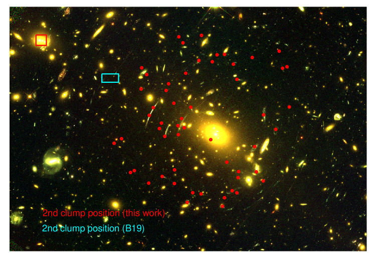
Figure 1: Core of AS 1063. Red circles represent the multiple images used in this work (see B19 for details). The boxes represent the location of the second mass clump associated with the north-east group. Size of the field equals 150$\arcsec$ $\times$ 96$\arcsec$. North is up, east is left.

Abell AS 1063 (a.k.a. RXJ 2248.7-4431), at redshift 0.348, has been observed deeply as part of the CLASH (Postman et al., 2012) and Hubble Frontier Fields (HFF, Lotz et al., 2017) programs. It is the only HFF cluster which looks unimodal and which is clearly dominated by a bright central galaxy.

If the dynamical state of the cluster has been debated, recent work combining X-ray and radio observations points out to a disturbed state, AS 1063 being in an early stage of merging (see Rahaman et al., 2021, and references therein).

3.1 Revisiting Bergamini et al. (2019) model

Following B19, we consider 55 multiple images coming from 20 sources (all spectroscopically confirmed).

We start by reproducing the B19 mass model, which includes an elliptical dPIE profile associated with the BCG, and a circular dPIE whose position is left free to vary in an area of 150$\arcsec$ $\times$ 120$\arcsec$ centred in the north-east region of the cluster where we can observe a galaxy group which generates additional strong lensing features for which no spectroscopic information is available, hence not considered. This mass clump has a vanishing core radius and a scale radius fixed to an arbitrary large value.

We do find the same parameters within the error bars and the same RMS, equal to 0.55$\arcsec$.

This mass model is able to reproduce accurately the observational constraints. However the location of the second clump does not coincide at all with the galaxy group in the North East (separation of 40$\arcsec$), although it was introduced to be associated with it (see cyan box on Fig. 1).

We revisit the B19 mass model. As mentioned above, we consider that having a mass clump whose position is not associated with a light concentration is not satisfactory. We force the position of this second mass clump to coincide with the light distribution of the most luminous galaxy of this group (red square on Fig. 1). We get an RMS of 0.67$\arcsec$. If the RMS gets larger by 0.12$\arcsec$, we prefer this mass model since each mass clump is associated with a luminous counterpart.

We then add an external shear component. This decreases the RMS to 0.53$\arcsec$. The strength of this external shear equals 0.03 and its position angle 40 degrees, pointing out to the north west direction. If it lowers the RMS by 0.14$\arcsec$, we prefer not including it in the mass model used to probe the underlying DM distribution. The main reason is that we do not observe any clear interpretation to this component (e.g. a mass concentration in the north west), therefore including this external shear might compensate for the limitations of the parametric modelling and eventually dilute the conclusions of our study, i.e. to disentangle between a cored and a non cored mass model. We will test and discuss that further.

Finally, we try a model for which the underlying mass distribution is described by a single mass clump, and find an RMS of 0.80$\arcsec$. We prefer a two clumps mass model (without external shear) since it has a physical interpretation. It constitutes the reference model from which we continue our investigations. Its parameters are given in Table 1. We note that the core radius is equal to 89.5$\pm$5.5 kpc, in agreement with previous studies.

3.2 Non cored mass model: a peaky DM distribution?

Following L16, we do investigate here if a non cored mass model for the main DM clump is also able to reproduce the observational constraints. We redo the modelling imposing the core radius to be smaller than 10 kpc, and obtain an RMS equal to 3.83$\arcsec$. Parameters are given in Table 1. The difference of RMS between the reference cored mass model and the non cored model equal 3.16$\arcsec$, which we consider large enough to favor a cored mass model. For this modeling, we have put a prior on the velocity dispersion of the second north east mass clump. Indeed, in the first attempts of testing a non cored mass model, we found that the velocity dispersion of the second mass clump was reaching values as high as 765 km s^-1 (instead of 350 km s^-1 for a cored mass model), which is somehow unrealistic given the optical richness and the absence of an X-ray associated emission (Bonamigo et al. 2018). Therefore, we decided to limit the velocity dispersion of the second mass clump to 450 km s^-1. As shown in Table 1, the value of this parameter is always stuck to this upper bound of the prior in non cored models. The RMS obtained without using this prior is 2.56$\arcsec$; this would lead to a difference of RMS equal to 1.89$\arcsec$. This highlights the importance of physically motivated priors.

Model	$\Delta$ ra	$\Delta$ dec	$e$	$\theta$	$\sigma$	$r_{\rm core}$	L∗ galaxy $\sigma$	L∗ galaxy $r_{s}$	RMS	$\sigma$ (2nd clump)
	$\arcsec$	$\arcsec$			km s-1	kpc	km s-1	kpc	$\arcsec$	km s-1
Cored	1.4$\pm$0.5	-0.9$\pm$0.4	0.64$\pm$0.01	141.1$\pm$0.5	1151$\pm$14	89.5$\pm$5.5	302$\pm$14	43$\pm$15.5	0.67$\arcsec$	350$\pm$50
Non Cored	1.2$\pm$0.5	1.5$\pm$0.6	0.7∗	138.9$\pm$0.7	963$\pm$5	10∗	303$\pm 15$	5∗	3.83$\arcsec$	450∗

Table 1: dPIE parameters inferred for the cored and the non cored models for the main clump describing AS 1063 (except the last column which corresponds to the velocity dispersion of the isothermal second clump), which has an arbitrary large scale radius $r_{s}$. Galaxy scale perturbers are described by dPIE profiles with vanishing core radii. Coordinates are given in arcseconds relative to $\alpha$ = 342.18321, $\delta$ = -44.530878; $e$ and $\theta$ are the ellipticity and position angle of the mass distribution. Error bars correspond to the 1$\sigma$ confidence level. Parameters with $*$ are stuck to a bound of the allowed prior.

3.3 Cosmology

In this work, we assume that the Universe is described by a flat Universe with $w_{\rm X}$ = -1 and $\Omega_{\rm M}$ = 0.3.

We run a cored and a non cored mass model, letting $w_{\rm X}$ and $\Omega_{\rm M}$ free. For each model, we compare the values of the optimized output cosmology with the values of the reference cosmology mentioned above. Our goal is to see if this test can help to discriminate between a cored and a non cored mass model. For the cored model, we get an RMS of 0.62$\arcsec$ (instead of 0.67$\arcsec$ for the reference model) and the reference cosmology is retrieved. For the non cored model, we get an RMS of 3.35$\arcsec$, and we do not retrieve the reference cosmology. In particular, $\Omega_{\rm M}$ is stuck to the lower bound allowed, i.e. 0. This test gives further credit to the non cored mass model. Note that we do not aim to constrain cosmology here but to provide an additional test in order to disentangle between a cored and a non cored mass model.

3.4 External shear

As mentioned above, an external shear component can compensate for the limitations of the parametric modelling and dilute the discrimination between a cored and a non cored mass model. The cored mass model with an external shear gives an RMS of 0.53$\arcsec$. For the non cored mass model, allowing an external shear component lowers the RMS to 3.07$\arcsec$ (versus 3.75$\arcsec$ when no external shear is allowed).

With the inclusion of an external shear component, the RMS difference equals to 2.54$\arcsec$. This is 0.5$\arcsec$ less discriminating compared to the case without any external shear.

3.5 Degeneracies with the BCG

We remove the BCG from the galaxy catalog and optimise it explicitly, in order to investigate any degeneracies between the main DM clump core radius and the BCG parameters. Its position is allowed to vary within $\pm$ 4$\arcsec$ from its centre and its core radius between 1 and 50 kpc. We use the values of B19 to put constraints on its velocity dispersion. B19 provide a gaussian prior with a mean and a standard deviation. We consider the same mean and the double of their standard deviation in order to allow for more freedom. We get an RMS equal to 0.64$\arcsec$. The optimized position is consistent with the centre of the light distribution. The ellipticity is unconstrained. Constraints on the core radius are very loose, the output PDF basically reproducing the prior, with a preference for the lower values. Therefore we see no degeneracies between the core radius of the BCG and the core radius of the main DM clump.

The value of the main DM clump core radius is consistent with the reference model.

4 MACS 0416

MACS 0416, at redshift 0.396, has been observed deeply as part of the HFF program.

4.1 Revisiting Bergamini et al. (2019) model

Recently, B19 and Bergamini et al. (2021) (B21 hereafter) presented two mass models for this cluster.

B19 reproduces 107 multiple images using a 3 DM mass clumps model with 193 galaxy members in the modelling, reaching an RMS of 0.61$\arcsec$. Each mass clump is associated with one of the three light concentrations of the cluster core (Fig. 2): one in the centre, associated with the BCG; one in the south west where a bright galaxy dominates; and one in the north east where three cluster members are located. They also optimize individually some parameters of two galaxies which are found to have an influence on some multiple images. We keep them in the models explored here and refer the reader to B19 for details.

B21 reproduces 182 multiple images using a 4 DM mass clumps model with 212 galaxy members in the modelling, reaching an RMS of 0.40$\arcsec$. This fourth mass component is located in the south west of the cluster core (Fig. 2). This makes two mass clumps in this area, none of them being clearly associated with the brightest galaxy located in this area. As discussed above, we consider that having DM clumps not associated with any luminous counterpart is not satisfactory, especially in this case where it improves the fit by only $\sim$0.1$\arcsec$.

Indeed, B21 also present three mass models which reproduce the 182 multiple images fairly well (RMS between 0.45$\arcsec$ and 0.48$\arcsec$ instead of 0.40$\arcsec$) where the DM is described using three mass clumps only. Using three other figures of merit (matching of the internal kinematics of the cluster members galaxies as well as BIC and AIC criteria), they choose the four mass clumps model as their reference model.

We also reproduce such a mass model where the 182 images are reproduced by a three mass clumps model with an RMS equal to 0.49$\arcsec$. The location of each mass clump is allowed to vary by $\pm$ 15$\arcsec$ from its luminous counterpart. We find each mass clump to coincide with its luminous counterpart even if not imposed. However, we note that the ellipticity of the two main DM clumps (the north east one being circular) is above 0.7 (0.84 and 0.73 respectively).

We then impose the ellipticity of each mass clump to be smaller than 0.7, and their positions to coincide with the light distribution (boxes on Fig. 2). For the central and south west mass clumps, positions are allowed to vary within $\pm$ 4$\arcsec$ from the centre of the associated bright galaxy. The north east mass clump position is allowed to vary within $\pm$ 3$\arcsec$ along the $x$ axis and within $\pm$ 4$\arcsec$ along the $y$ axis from the centre of the associated luminous counterpart.

The RMS equals to 0.63$\arcsec$. The core radii of each mass clump is equal to 41.5$\pm$2.7; 51.2$\pm$3.7 and 60.4$\pm$8.6 kpc respectively. The ellipticity of the main and north-east mass distributions are stuck to 0.7. This model constitutes the reference model from which we continue our investigations. Its parameters are given in Table 2.

Similar three clumps mass models have also been proposed by Jauzac et al. (2014) and Richard et al. (2021). We show on Fig. 2 the positions of the mass clumps inferred in their analysis.

Cored Model	$\Delta$ ra	$\Delta$ dec	$e$	$\theta$	$\sigma$	$r_{\rm core}$
	$\arcsec$	$\arcsec$			km s-1	kpc
Clump 1	-1.8$\pm$0.5	0.4$\pm$0.3	0.69$\pm$0.01	143.3$\pm$1.0	629$\pm$16	41.5$\pm$2.7
Clump 2	22.3$\pm$0.4	-39.4$\pm$0.4	0.69$\pm$0.01	127.3$\pm$0.8	769$\pm$20	51.2$\pm$3.7
Clump 3	-32.2$\pm$0.5	12∗	0.40$\pm$0.09	72$\pm$9	369$\pm$22	60.4$\pm$8.6

Table 2: dPIE parameters inferred for the reference cored model of MACS 0416, with an RMS equal to 0.63$\arcsec$. Coordinates are given in arcseconds relative to $\alpha$ = 64.0381417, $\delta$ = -24.0674722; $e$ and $\theta$ are the ellipticity and position angle of the mass distribution. Error bars correspond to the 1$\sigma$ confidence level. Parameters with $*$ are stuck to a bound of the allowed prior. For an L* galaxy, we have $\sigma$ = 237$\pm$10 km s^-1 and $r_{s}$ = 10$\pm$2 kpc.

4.2 Non cored mass model

We redo the modelling imposing the core radius of each mass clump to be smaller than 10 kpc.

We get an RMS equal to 2.07$\arcsec$. This is 1.44$\arcsec$ worse than the cored mass model, which is substantial. A cored mass model is therefore clearly preferred but this difference of RMS is not enough to disentangle between a cored and a non cored model according to the (somehow arbitrary) criteria proposed in Section 2.4. The ellipticity of the main and north-east mass distributions are also stuck to 0.7. The core radii of the three mass clumps are stuck to 10 kpc. All parameters are given in Table 3.

Non Cored Model	$\Delta$ ra	$\Delta$ dec	$e$	$\theta$	$\sigma$	$r_{\rm core}$
	$\arcsec$	$\arcsec$			km s-1	kpc
Clump 1	-1.1$\pm$0.3	-0.1$\pm$0.2	0.7∗	135.4$\pm$0.6	522$\pm$4	10∗
Clump 2	21.6$\pm$0.2	-37.4$\pm$0.4	0.7∗	129.6$\pm$0.8	651$\pm$5	10∗
Clump 3	-32.1$\pm$0.1	12.9$\pm$0.1	0.27$\pm$0.08	126.5$\pm$9.0	357$\pm$8	10∗

Table 3: Same as Table 2 for the non cored model of MACS 0416, with an RMS equal to 1.88$\arcsec$. For an L* galaxy, we have $\sigma$ = 240$\pm$5 km s^-1 and $r_{s}$=108 kpc (stuck to the upper bound of the allowed prior).

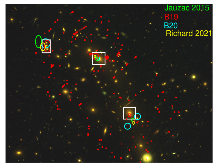
Figure 2: Core of MACS 0416. Red circles represent the multiple images used in this work (see B19 for details). Location of the mass clumps from different studies are shown by ellipses, whose size represent the 1$\sigma$ error bar on the position. White boxes represent the priors on the position of each DM clump. North is up, east is left. Size of the field equals to 137$\arcsec$ $\times$ 105$\arcsec$.

4.3 Cosmology

We run a cored and a non cored mass model, letting $w_{\rm X}$ and $\Omega_{\rm M}$ free. For each model, we compare the values of the optimized output cosmology with the values of the reference cosmology mentioned above.

For the cored model, we get RMS = 0.51$\arcsec$ (instead of 0.63$\arcsec$ for the reference model) and the cosmology is off ($\Omega_{\rm M}$ = 0.16$\pm$1.0, $w_{\rm X}\,<$1.3). For the non cored model, we get RMS = 1.74$\arcsec$, and the cosmology is totally off, basically unconstrained.

This test does not gives further insights to disentangle between a cored and a non cored mass model.

5 MACS J1206

MACS J1206 is a unimodal cD dominated galaxy cluster located at redshift 0.439. Although considered as dynamically relaxed (Sereno 2017), the smooth component (DM + hot gas) shows a significant asymmetry.

5.1 Revisiting Bergamini et al. (2019) model

B19 reproduce 82 multiple images using a mass distribution composed of three dark matter haloes, three dPIE clumps to model the X-ray surface brightness (Bonamigo et al., 2018), a strong external shear ($\gamma_{\rm ext}=0.12$) of unknown origin and 258 haloes describing the cluster members. This set of multiple images is well reproduced (RMS = 0.46$\arcsec$).

The positions of the three DM clumps are illustrated in Fig. 3 (cyan ellipses). If one of these mass clumps is coincident with the cD galaxy, the others are not associated with any luminous counterpart. Their core radii equal to 37, 82 and 69 kpc (central, eastern and western clumps respectively). B19 state that these DM clumps are necessary to reproduce the apparent elongated asymmetry of the cluster. A similar mass model, in terms of number and position of DM clumps, has been presented by Richard et al. (2021), reaching an equivalent RMS.

Such a three clumps mass model was already proposed in the study by Caminha et al. (2017), who noted that these ”multi mass components should not be associated with extra DM haloes, but rather to extra asymmetries or high order multipoles that a single parametric profile cannot account for”.

If we assume that the mass distribution is described by a single dPIE mass clump associated with the cD galaxy plus the galaxy component and the X-ray gas and perform the mass modelling, we end up with an RMS of 2.24$\arcsec$. Looking at the mass clump parameters, we find that the ellipticity is stuck to the higher bound allowed (0.7) and that the core radius is constrained to 74$\pm$3 kpc.

The RMS difference between the former two models, equal to 1.8$\arcsec$, favors a three mass clumps model. We consider that such a three clumps model is not satisfactory and we conclude that the SL constraints in MACS J1206 are not well reproduced by a single halo described parametrically.

With the goal to present a physically motivated parametric mass model for MACS J1206, we pursue our investigations.

5.2 A two clumps mass model

We notice that there is a bright galaxy east of the BCG (yellow box on Fig. 3) with which we associate a DM clump. We impose the centre of this mass component to be within $\pm$ 2$\arcsec$ from the centre of the associated luminous component, i.e. within the yellow box on Fig. 3. We also allow for an external shear component.

We end up with an RMS equal to 1.45$\arcsec$. The main DM clump has a core radius equal to $\sim$ 35 kpc and has a high but reasonable ellipticity ($\sim$ 0.6). On the other hand, the second DM clump is extremely flat, with a core radius reaching the higher bound of the prior equal to 230 kpc.

5.3 A three clumps mass model

North west of the BCG is another bright galaxy (yellow box on Fig. 3) with which we associate a DM clump, investigating a three clumps mass model. We impose the centre of this mass component to be within $\pm$ 2$\arcsec$ from the centre of the associated luminous component, and allow for an external shear component.

The resulting RMS equals to 1.38$\arcsec$. Parameters of the main DM clump are compatible with the one obtained in the case of the two clumps mass model, but the two other DM clumps display very flat mass profiles, with core radii equal to 190 and 230 kpc for the east and north west clumps respectively.

5.4 A four clumps mass model

South west of the BCG is another bright galaxy (yellow box on Fig. 3) with which we associate a DM clump, investigating a four clumps mass model. We impose the centre of this mass component to be within $\pm$ 2$\arcsec$ from the centre of the associated luminous component, and allow for an external shear component.

The resulting RMS equals to 1.19$\arcsec$. Parameters of the main DM clump are compatible with the one obtained in the case of the two clumps mass model. The other three DM clumps display very flat mass profiles, with core radii equal to 172, 200 and 145 kpc respectively.

In all cases, we find that the inclusion of an external shear allows to lower the RMS by $\sim$ 0.6$\arcsec$. Its value is $\sim$ 0.06.

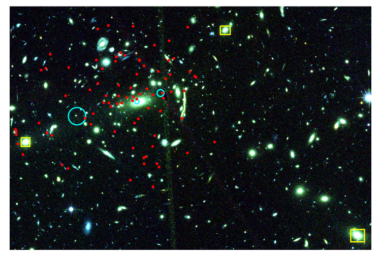
Figure 3: Core of MACS J1206. Red circles represent the multiple images used in this work (see B19 for details). Location of the three mass clumps proposed by B19 are shown by cyan ellipses, whose size represent the 1$\sigma$ error bar on the position. Yellow boxes represent the prior on the position of the mass clumps included in the different mass model investigated. North is up, east is left. Size of the field equals to 166$\arcsec$ $\times$ 110$\arcsec$.

We see that we are able to lower the RMS by adding extra clumps which we associate with some light concentrations. The more associations, the lower the RMS. However, we are not able to get an RMS lower than 1$\arcsec$. We also find that these extra mass clumps do require very large core radii, between 145 and 230 kpc.

We conclude from this serie of tests that MACS J1206 cannot be reliably described by a pure parametric model where each mass component would be associated with a luminous counterpart.

6 Improving Parametric Mass Modelling with mild Perturbations

We see that in the case of MACS J1206, the parametric approach reaches its limit and does not allow to provide a physically motivated parametric description of the mass distribution.

We aim to see if adding a (mild) perturbation to the parametric modelling could help to provide a decent fit. Our main concern is whether adding this perturbation might make us lose the advantages of the parametric mass modelling, i.e. if we end up with clumps parameters that are biased by the perturbation, preventing us from doing cluster physics.

Recently, something along this line has been implemented in Lenstool (Beauchesne et al., 2021). This functionality consists in a surface of 2D B-spline functions added on top of the lensing potential. While it has been shown to provide enhancement to the reconstruction of a simulated cluster, this is the first time that it is applied on observational data. In comparison to the free-form approach developed in Jullo & Kneib (2009), this perturbative patch cannot reproduce a full mass distribution and has to be combined with other analytical potentials. Indeed, its total mass is always null, and it rather redistributes the one from the other model components. If complex grids of B-spline functions are possible, the current implementation is limited to a squared regular mesh. But as the perturbation should be small in comparison to the total mass model, the induced biases can be neglected. Besides, the grid does not need more knowledge than the size of the constrained area to be built such as an existing mass model or the light distribution.

We first test the inclusion of such perturbations on AS 1063 which is already well described by a parametric mass model, then we use them on MACS J1206.

6.1 Test on AS 1063

We choose AS 1063 in order to test this approach and see how the reference mass model presented in Section 3.1 responds to the inclusion of the perturbation.

We perform a mass model for AS 1063 as in Section 3, including the B-spline perturbation. We use the same scheme of priors as in Beauchesne et al. (2021) with a minimal lattice size of  $105\arcsec$ and a grid of $5\times 5$ basis functions. However, we kept the previous uniform priors for the dPIE parameters. The resulting RMS equals to 0.36$\arcsec$, an improvement by almost a factor of two when compared with the pure parametric mass model (0.67$\arcsec$).

We compare the parameters of the reference model (Table 1) with the parameters obtained when adding the perturbation. They do agree within the 3$\sigma$ error bars. This test suggests that the B-spline perturbation is able to improve the pure parametric fit (as shown in Beauchesne et al., 2021). Besides, this test also suggests that it is mild enough so that the parameters of the associated parametric mass model are not significantly modified.

We also run a non cored mass model, including the B-spline perturbation. The goal is to see if the perturbation is able to provide a decent non cored mass model. In other words, is the perturbation able to compensate for the apparent need of a core in the centre?

We find an RMS of 1.50$\arcsec$, instead of 3.83$\arcsec$ when not using the perturbation. Comparing the outputs of these two models, we find that the main DM clump parameters do agree with each other within the 3$\sigma$ error bars, once again suggesting that the perturbation is mild enough not to significantly modify the parameters of the parametric model. Besides, given the value of the RMS, we find that the perturbation is not able to compensate for the need of a core in the centre. In addition, the associated 2D mass map (Fig. 4, upper left panel) has an irregular shape. If the parameters of the associated parametric model are not significantly modified by the inclusion of the perturbation, we note that the resulting total mass map appears unphysical. Given the resulting shape of the mass map, we do not consider this mass model as ”physically relevant” and do not use it for further investigations.

We show the 2D mass maps associated with each model on Fig. 4. Considering the mass maps corresponding to the models including the perturbation, we see that when the fit is good (RMS=0.36$\arcsec$), the shape of the mass contours are physically relevant, whereas they look unphysical when the fit is bad (RMS=1.50$\arcsec$).

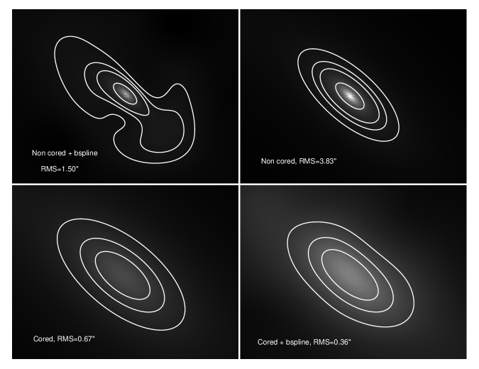
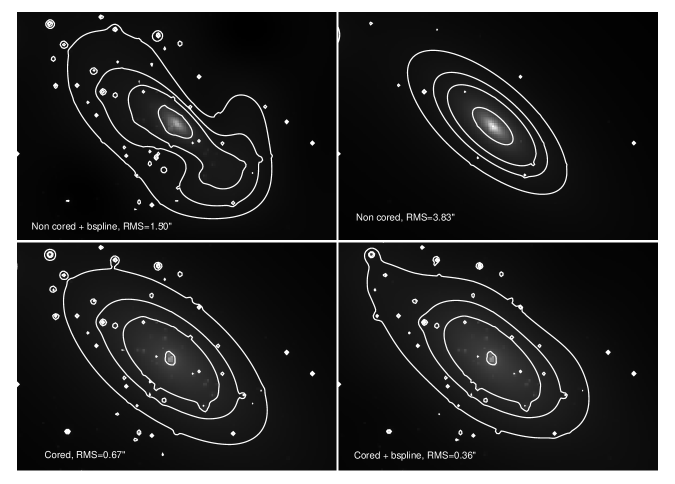
Figure 4: 2D mass maps (contours equal to 0.03, 0.04, 0.05 and 0.1 10¹² M_☉ arcsec^-2) for the different models explored here for AS 1063. The size of each panel equals to 140$\arcsec$$\times$107$\arcsec$, centred on the cD galaxy. Top: we show the 2D mass distribution corresponding to the main DM halo + the B-spline perturbation when included. Bottom: on top of the main DM halo and the perturbation, we add the individual galaxies.

We also test this approach on MACS 0416, investigating how the reference mass model presented in Section 4.1 responds to the inclusion of the perturbation. The resulting RMS equals to 0.46$\arcsec$ (versus 0.63$\arcsec$ for the reference model). Besides, as for AS 1063, the parameters obtained agree within the 3$\sigma$ error bars with the one obtained without the B-spline perturbation.

The results from these tests are encouraging enough to apply the perturbation on MACS J1206.

6.2 Application on MACS J1206

6.2.1 A cored mass model allowing for the perturbation

On top of the single central DM clump, we consider a B-spline perturbation. No external shear is added. We end up with an RMS equal to 0.53$\arcsec$ (instead of 2.24$\arcsec$ without the perturbation nor external shear, see Section 5.1).

Allowing for an external shear component does not improve the fit. B-spline coefficients differ, suggesting that an external shear component can be described by the B-spline perturbation instead. Comparing the parameters of the main DM clump obtained with and without the perturbation, we find that they do agree. Indeed, comparing the output PDFs for each parameters, we find that all parameters but one do agree within the 3$\sigma$ error bars. Only the position of the main clump along the X axis disagree between the two models. This disagreement is small, equal to 5 kpc. We find that the perturbation is able to provide a decent fit without modifying the parametric part, allowing to keep the advantages of the pure parametric mass modelling.

Parameters of the main DM clump (when the perturbation is included) are given in Table 4. In particular, we do find a core radius equal to 57.4$\pm$1.7 kpc.

6.2.2 Non cored mass model

Keeping the perturbation in the modelling, we then impose the core radius to be smaller than 10 kpc. The resulting RMS equals 7.39$\arcsec$. Parameters are given in Table 4. The difference in RMS is substantial, equal to 6.83$\arcsec$, which is large enough to favor a cored mass model for MACS J1206. The associated mass map displays an unphysical shape (Fig. 5).

Model	$\Delta$ ra	$\Delta$ dec	$e$	$\theta$	$\sigma$	$r_{\rm core}$	L∗ galaxy $\sigma$	L∗ galaxy $r_{s}$	RMS
	$\arcsec$	$\arcsec$			km s-1	kpc	km s-1	kpc	$\arcsec$
Cored	1.7$\pm$0.4	0.5$\pm$0.2	0.62$\pm$0.01	12.3$\pm$0.3	1071$\pm$7	57.4$\pm$1.7	266$\pm$6	41$\pm$4.6	0.53$\arcsec$
Non Cored	1.7$\pm$0.2	1.3$\pm$0.2	0.7∗	18.2$\pm$1.0	909$\pm$8	10∗	253$\pm 2$	92$\pm$12.0	7.39$\arcsec$

Table 4: dPIE parameters inferred for the cored and the non cored models for MACS J1206, when the bspline perturbation is included. Coordinates are given in arcseconds relative to $\alpha$ = 181.55062, $\delta$ = -8.8009361; $e$ and $\theta$ are the ellipticity and position angle of the mass distribution. Error bars correspond to the 1$\sigma$ confidence level. Parameters with $*$ are stuck to a bound of the allowed prior.

6.2.3 Additional Tests

Keeping the core radius smaller than 10 kpc, we test what happens if we do not include the B-spline perturbation. We end up with an RMS equal to 11$\arcsec$.

Adding an external shear component lowers the RMS to 9.4$\arcsec$. The value of this external shear is stuck to 0.1, the upper bound allowed by the prior (Section 2.3). Interestingly, if we allow this external shear to reach higher values, it ends up to be constrained to 0.26, a very unrealistic value since it is comparable to what would be experienced at 100$\arcsec$ from the centre of galaxy cluster Abell 1689 (Limousin et al., 2007b). In this case the RMS lowers to 2.4$\arcsec$. This highlights once again the importance of providing well motivated priors in SL mass modelling.

In Fig. 5, we show the 2D mass maps corresponding to the different models of MACS J1206 explored. As for AS 1063, considering the mass maps corresponding to the models including the perturbation, we see that when the fit is good (RMS=0.53$\arcsec$), the shape of the mass contours are physically relevant, whereas they look unphysical when the fit is bad (RMS=7.39$\arcsec$).

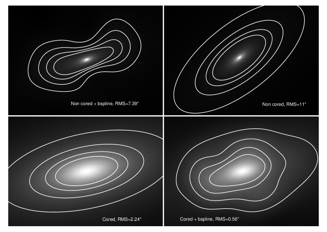
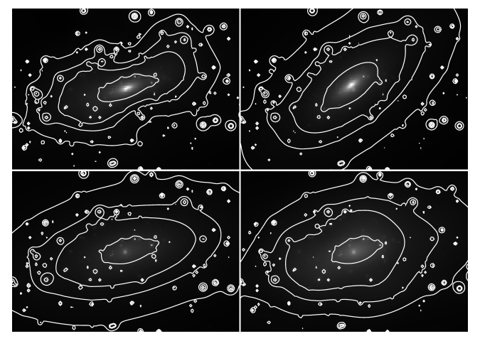
Figure 5: 2D mass maps for the different models explored here for MACS J1206. For clarity, we label these models on the four top mass maps only. Same labels apply for the four bottom maps. The size of each panel equals to 150$\arcsec$$\times$105$\arcsec$, centred on the cD galaxy. Top: we show the 2D mass distribution corresponding to the main DM halo + the B-spline perturbation when included. Contours equal to 0.02, 0.03, 0.04, and 0.05 10¹² M_☉ arcsec^-2. Bottom: on top of the main DM halo and the perturbation, we add the individual galaxies. Contours equal to 0.02, 0.03, 0.04, and 0.08 10¹² M_☉ arcsec^-2.

6.3 Degeneracies with the BCG

We remove the BCG from the galaxy catalog and optimise it explicitly, in order to investigate any degeneracies between the main DM clump core radius and the BCG parameters. The B-spline perturbation is considered in the modelling. The position of the BCG is allowed to vary within $\pm$ 4$\arcsec$ from its centre and its core radius between 1 and 50 kpc. We use the values of B19 to put constraints on its velocity dispersion. B19 provide a gaussian prior with a mean and a standard deviation. We consider the same mean and the double of their standard deviation in order to allow for more freedom.

We get an RMS equal to 0.50$\arcsec$. The optimized position of the BCG is consistent with the light distribution. Its ellipticity reaches the upper bound of the prior, and its core radius is constrained to be smaller than 5 kpc. The parameters of the main DM halo are consistent with the one obtained without optimising the BCG individually. Its core radius is found a bit larger in this case (14” instead of 13”). We see no degeneracies between the core radius of the BCG and the core radius of the main DM clump.

6.4 Cosmology

We consider the cored mass model presented in Table 4 and let the cosmology free. The RMS equals to 0.53$\arcsec$ and the reference cosmology is retrieved (Fig. 8, Left panel). Doing the same exercise with the non cored mass model, the RMS equals to 2.3$\arcsec$ (versus 7.39$\arcsec$). The resulting cosmology is off, with $\Omega_{\rm M}$ $\sim$ 0.

This test gives additional support to the non cored mass model.

6.5 Comparison with B19

In Fig. 7, we compare the 2D total mass map we obtain for MACS J1206 with the one proposed by B19. We see that they have similar shapes: the model presented here is very close to the one proposed by B19 in term of 2D total mass map. This shows that the perturbation is able to reproduce the asymmetry given by the B19 three clumps mass model using only one single mass clump.

We integrate the mass maps starting at the BCG centre in order to derive the 1D mass profile. The error bars are computed from the MCMC realizations. We present the mass profile in the radial range where multiple images can be found, i.e. up to $\sim$ 320 kpc from the centre. As expected, we find they both agree with each other (Fig. 6).

Both mass model fully agree in term of total mass (both 2D maps and 1D integrated profile), which is expected since the lensing constraints are sensitive to the total mass. However, we have two very different ways of constructing this total mass, in term of the underlying smooth DM component (the galaxy scale perturbers being fixed to the same values thanks to the B19 results). When B19 propose a three clumps mass model plus an external shear component, we propose a one clump mass model with a perturbation.

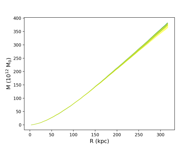
Figure 6: Comparison between the integrated mass profile: B19 in green and the one presented in this work in yellow. The 3$\sigma$ error bars are computed from the MCMC realizations.

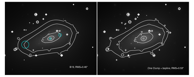
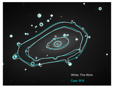
Figure 7: Comparison between the 2D mass map presented in this work (Upper Right) and the one obtained by B19 (Upper Left) for MACS J1206. Lower Pannel: We overplot the mass contours corresponding to both studies. The size of each panel equals to 101$\arcsec$$\times$77$\arcsec$, centred on the cD galaxy. Contours equal to 0.05, 0.06, 0.1, and 0.13 10¹² M_☉ arcsec^-2. Cyan ellipses represent the location of the three mass clumps proposed by B19, as in Fig. 3.

To further compare both models, we let the cosmological parameters free during the optimisation. For the one clump cored mass model presented in this work, we consider the results obtained in Section 6.5 where it is shown that the reference cosmology is retrieved. We consider the mass model published by B19 and let the cosmology free during the optimisation. To obtain stable results, we need to lower the rate value to 0.005. We obtain an RMS equal to 0.43$\arcsec$, and the reference cosmology is not retrieved. Constraints in the ($\Omega_{\rm M},w_{\rm X}$) plane are compared in Fig. 8.

These two mass models are likely to provide different estimates of the magnification. Indeed, different mass distributions lead to different estimates of the magnification experienced by background sources. In MACS J0717, we found that the cored and the non cored mass models lead to different magnification estimates, adding a systematic error that is in general larger than the statistical error derived from a given mass model. A thorough investigation of the difference of magnification computed using the model presented here and the one by B19 is beyond the scope of this paper, but it should be taken into account if using MACS J1206 as a gravitational telescope, as it might decrease the area of the image plane where magnification are well determined enough for reliable studies of the high-redshift Universe.

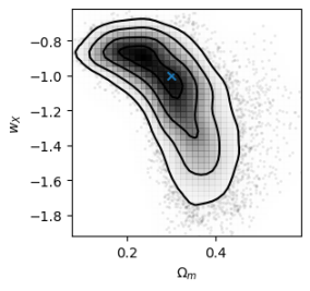
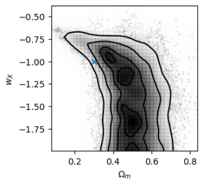
Figure 8: Comparison between the constraints obtained on the cosmological parameters using the reference model presented in Table 4 (Left) and the one obtained when using the B19 model (Right). The cyan cross represents the reference cosmology.

7 Discussion

We summarize the results presented in this paper in Table 5.

Model	RMS	$\Delta(\rm RMS)$	$r_{\rm core}$
	$\arcsec$	$\arcsec$	kpc
AS 1063, cored	0.67	3.16	89.5$\pm$5.5
AS 1063, non cored	3.83	–	–
MACS 0416, cored	0.63	1.44	41.5$\pm$2.7; 51.2$\pm$3.7; 60.4$\pm$8.6
MACS 0416, non cored	1.88	–	–
MACS J1206, cored	0.53	6.86	57.4$\pm$1.7
MACS J1206, non cored	7.39	–	–

Table 5: Summary of the results presented in this paper. For each cluster, we report the RMS obtained for both the cored and the non cored model, as well as the difference of RMS between the non cored and the cored mass model. B-spline perturbations are used in the case of MACS J1206 only.

7.1 Physically Motivated Parametric Mass Modelling

In this work, we choose to present mass models which are physically motivated. In particular, we want to avoid the inclusion of large scale DM clumps having no luminous counterpart, even if this might degrade the SL fit. Therefore we impose a strong prior on the position of the large scale DM clumps. We prefer conclude that a parametric mass modelling is not adapted to describe a cluster instead of using ”adhoc dark clumps” whose physical interpretation is misleading. In these cases, a non parametric approach might be considered instead. In between, we have shown that using a mild perturbation in the form of B-splines is useful to get a good fit while at the same time keeping the advantages of the pure parametric mass modelling.

Along this line, we have also considered other well motivated priors, even though they do sometimes degrade the quality of the fit. This is the case when including the X-ray component explicitly in AS 1063. This is also the case when limiting the strength of the external shear component in MACS J1206.

7.2 On the inner shape and nature of DM

We have investigated the inner shape of the DM distribution in a sample of three massive galaxy clusters. In all cases, a cored mass distribution is preferred over a non cored mass distribution. This is a potentially very exciting result, since it might be a signature of SIDM. Prudently enough, we do not make any strong claims of evidence for SIDM. This would require performing this kind of analyses on more galaxy clusters; doing rigorous tests with simulated data and exploring other ways to improve the models within the standard Cold Dark Matter paradigm. In particular, not fully understood interactions between baryons and dark matter can lead to core formation.

In two cases, the RMS difference is larger than 2$\arcsec$, which we consider large enough in order to disentangle between a cored and a non cored mass distribution. Actually it is even larger than 3$\arcsec$. In AS 1063, the RMS difference equals to 3.16$\arcsec$ and the core radius equals to 89.5$\pm$5.5 kpc. In MACS J1206, the RMS difference equals to 6.83$\arcsec$ and the core radius equals to 57.4$\pm$1.7 kpc. In MACS 0416, the RMS difference equals to 1.44$\arcsec$ and the core radius of each clump equals to 41.5$\pm$2.7 kpc, 51.2$\pm$3.7 kpc and 60.4$\pm$8.6 kpc.

Note that we do not try to model AS 1063 & MACS J1206, the two unimodal clusters studied here, using an NFW mass profile which is non cored by definition. This is because we do not observe multiple images at radius large enough to constrain the typical size of the scale radius for a cluster scale NFW halo. Ongoing BUFFALO observations (Steinhardt et al., 2020), in particular the weak lensing data, might help to test if a NFW mass profile is able to reproduce the weak+strong lensing data for AS 1063.

These values are summarized in Table 5. We note that some of them are at the higher bound (AS 1063) of what seems to be allowed in an SIDM scenario. As discussed in the introduction, a thorough investigation of core radii within an SIDM scenario is still lacking.

Regarding SIDM, an observable consequence would be oscillations of the BCG around the centre of the halo after mergers, which could persist for several Gyr (Kim et al., 2017). For the unimodal clusters studied here (AS 1063 and MACS J1206), we find an offset between the BCG and the DM smaller than $\sim$3 kpc, which is compatible with a CDM scenario with no self interactions (Harvey et al., 2019).

Recent study by Andrade et al. (2021) presented a SL analysis of AS 1063 using a cored NFW mass profile. It is not straightforward to compare the values of the core radius for such an NFW profile and the core radius of a dPIE profile. However, Andrade et al. (2021) do find evidence for a core radius equal to 19.83${}^{+13.03}_{-9.41}$ kpc. These authors do study a sample of 8 regular galaxy clusters, out of which three do have a core strictly larger than 0.

However, another recent study by Sartoris et al. (2020) performing a joint fit to the velocity dispersion profile of the BCG and to the velocity distribution of cluster member galaxies over a radial range from 1 kpc to the virial radius determine the inner slope of AS 1063 to be fully consistent with the NFW predictions.

7.3 Relaxing the B19 priors

In MACS 0717, it was found that the degeneracies between the smooth and the galaxy scale components prevented to disentangle between a cored and a non cored mass model. In this work we have been using priors on the galaxy scale component coming from spectroscopic observations. For each cluster studied here, we have relaxed the priors by B19, using flat priors for the velocity dispersion and scale radius instead of the B19 results, as it is usually done in SL modelling. The velocity dispersion is allowed to vary between 110 and 350 km s^-1 and the scale radius between 5 and 150 kpc.

We present in Table 6 the results for each cluster, for both the cored and the non cored mass models, in terms of RMS and parameters of the galaxy scale perturbers.

Model	$r_{s}$	$\sigma$	RMS	$\Delta(\rm RMS)$
	kpc	km s-1	$\arcsec$	$\arcsec$
AS 1063, cored	150 (43)	230 (302)	0.64 (0.67)	3.07 (3.16)
AS 1063, non cored	5 (5)	100 (303)	3.71 (3.83)	-
MACS 0416, cored	42 (10)	264 (237)	0.62 (0.63)	1.18 (1.44)
MACS 0416, non cored	42 (10)	201 (237)	1.80 (2.07)	-
MACS J1206, cored	29 (41)	295 (266)	0.52 (0.53)	1.81 (6.83)
MACS J1206, non cored	150∗ (92)	297 (253)	2.33 (7.49)	-

Table 6: Results obtained on the galaxy scale perturbers when relaxing the B19 priors, for the different models explored. We also report the RMS obtained and the difference of RMS between the non cored and the cored mass model. Values into brackets correponds to the results obtained when considering the B19 priors.

In MACS J1206, we found that the B19 priors are important and actually allow to discriminate between a cored and a non cored mass model. We do not understand why these priors do help in MACS J1206 but not in AS 1063 and MACS 0416. In the former two clusters, it is important to note that including these priors is essential since it provides more realistic parameters for the galaxy scale perturbers and therefore gives more reliability to the results obtained on the inner shape of the DM distribution in these clusters as we are confident that they are not driven by the degeneracies between the smooth and the galaxy scale components.

We stress that this study by B19 is a major step forward and is paving the road towards more realistic SL mass modelling. With the development of spectrographs like MUSE, we will have more and more clusters with spectroscopic data for galaxy scale perturbers to be included in SL modelling.

7.4 Inclusion of the X-ray gas component

For each cluster studied here, we do investigate a model where the X-ray gas component is not explicitly included in the modelling. For AS 1063, the RMS equals 0.60$\arcsec$ instead of 0.67$\arcsec$ for the reference model. The parameters of both models agree within 1$\sigma$, except for the velocity dispersion of the main clump, which is about 100 km s^-1 larger when the X-ray component is not included.

For MACS 0416, the RMS equals 0.57$\arcsec$ instead of 0.63$\arcsec$. The parameters of both models for the different clumps agree within the 3$\sigma$ error bars. The velocity dispersion of the north-east clump is found slightly higher when the X-ray component is not included (437$\pm$34 vs 369$\pm$22 km/s).

For MACS 1206, the RMS equals 0.67$\arcsec$ instead of 0.53$\arcsec$. The parameters of both models for the main clump agree within the 3$\sigma$ error bars, except for the velocity dispersion, which is a bit larger to compensate (1158 km s^-1 versus 1071 km s^-1).

For AS 1063 and MACS 0416, the RMS is slightly better when not including the X-ray gas component. Therefore, if looking at the best possible RMS, one might be tempted to favor a mass model where the X-ray component is not included. However we observe this component in X-ray, therefore it is worth including it even if the description is not the best possible. This illustrates the question raised in the introduction of this paper about the balance between having the best fit possible and presenting a physically motivated mass model.

Ultimately, we might want to fit simultaneously the lensing constraints and the X-ray data so that the RMS becomes more representative of the inclusion of the X-ray component.

7.5 On the choice of priors

During an optimisation process, Lenstool always provides an answer, i.e. some best fit parameters describing a mass distribution. But Lenstool, as any other modelling algorithm, does not care about the physical relevance of the outputs. This is where expertise from the modeller comes into play. Actually, we have seen that different modellers using the same set of data and the same modelling algorithm can end up with different answers (Meneghetti et al., 2017).

The parameter space being sometimes very large, it can be relevant to limit it by imposing well motivated priors. Actually we always provide priors on each parameters, i.e. a range within which they are allowed to vary. The tightness of this range depends on the availability of constraints coming from other probes or from theory. For example, in this work we have used the constraints obtained by B19 in order to put a prior on the galaxy scale perturbers.

We have seen at different occasions how the choice of priors does change the best model inferred from the analysis.

Related to the choice of priors is the quest for the best fit. Of course we want the RMS to be as low as possible, and definitely below a given threshold (assumed here to be 1$\arcsec$). However, we have seen in this paper that sometimes a mass model can provide a better fit but at the same time be unrealistic.

With this work, we aim to provide the following working hypothesis worth considering in parametric mass modelling:
First, any large scale mass clump should be associated with a light counterpart. Second, any well motivated prior should be included.

References

- Acebron et al. (2022) Acebron, A., Grillo, C., Bergamini, P., et al. 2022, ApJ, 926, 86
- Acebron et al. (2017) Acebron, A., Jullo, E., Limousin, M., et al. 2017, Monthly Notices of the Royal Astronomical Society, 470, 1809–1825
- Acebron et al. (2020) Acebron, A., Zitrin, A., Coe, D., et al. 2020, The Astrophysical Journal, 898, 6
- Andrade et al. (2021) Andrade, K. E., Fuson, J., Gad-Nasr, S., et al. 2021, Monthly Notices of the Royal Astronomical Society, 510, 54–81
- Beauchesne et al. (2021) Beauchesne, B., Clément, B., Richard, J., & Kneib, J.-P. 2021, Monthly Notices of the Royal Astronomical Society, 506, 2002–2019
- Bergamini et al. (2019) Bergamini, P., Rosati, P., Mercurio, A., et al. 2019, Astronomy & Astrophysics, 631, A130
- Bergamini et al. (2021) Bergamini, P., Rosati, P., Vanzella, E., et al. 2021, Astronomy & Astrophysics, 645, A140
- Bonamigo et al. (2018) Bonamigo, M., Grillo, C., Ettori, S., et al. 2018, The Astrophysical Journal, 864, 98
- Caminha et al. (2017) Caminha, G. B., Grillo, C., Rosati, P., et al. 2017, Astronomy & Astrophysics, 607, A93
- Caminha et al. (2019) Caminha, G. B., Rosati, P., Grillo, C., et al. 2019, Astronomy & Astrophysics, 632, A36
- Cerny et al. (2018) Cerny, C., Sharon, K., Andrade-Santos, F., et al. 2018, The Astrophysical Journal, 859, 159
- Cibirka et al. (2018) Cibirka, N., Acebron, A., Zitrin, A., et al. 2018, The Astrophysical Journal, 863, 145
- Despali et al. (2016) Despali, G., Giocoli, C., Bonamigo, M., Limousin, M., & Tormen, G. 2016, Monthly Notices of the Royal Astronomical Society, 466, 181–193
- Elíasdóttir et al. (2007) Elíasdóttir, Á., Limousin, M., Richard, J., et al. 2007, ArXiv e-prints, 710
- Fischer et al. (2021) Fischer, M. S., Brüggen, M., Schmidt-Hoberg, K., et al. 2021, Monthly Notices of the Royal Astronomical Society, 505, 851–868
- Harvey et al. (2019) Harvey, D., Robertson, A., Massey, R., & McCarthy, I. G. 2019, Monthly Notices of the Royal Astronomical Society, 488, 1572–1579
- Host (2012) Host, O. 2012, MNRAS, 420, L18
- Irastorza & Redondo (2018) Irastorza, I. G. & Redondo, J. 2018, Progress in Particle and Nuclear Physics, 102, 89–159
- Jauzac et al. (2014) Jauzac, M., Clément, B., Limousin, M., et al. 2014, MNRAS, 443, 1549
- Jauzac et al. (2015) Jauzac, M., Richard, J., Jullo, E., et al. 2015, MNRAS, 452, 1437
- Jullo & Kneib (2009) Jullo, E. & Kneib, J. 2009, MNRAS, 395, 1319
- Jullo et al. (2007) Jullo, E., Kneib, J.-P., Limousin, M., et al. 2007, New Journal of Physics, 9, 447
- Kim et al. (2017) Kim, S. Y., Peter, A. H. G., & Wittman, D. 2017, Monthly Notices of the Royal Astronomical Society, 469, 1414–1444
- Lagattuta et al. (2019) Lagattuta, D. J., Richard, J., Bauer, F. E., et al. 2019, Monthly Notices of the Royal Astronomical Society
- Limousin et al. (2007a) Limousin, M., Kneib, J. P., Bardeau, S., et al. 2007a, A&A, 461, 881
- Limousin et al. (2005) Limousin, M., Kneib, J.-P., & Natarajan, P. 2005, MNRAS, 356, 309
- Limousin et al. (2016) Limousin, M., Richard, J., Jullo, E., et al. 2016, Astronomy & Astrophysics, 588, A99
- Limousin et al. (2007b) Limousin, M., Richard, J., Jullo, E., et al. 2007b, ApJ, 668, 643
- Lotz et al. (2017) Lotz, J. M., Koekemoer, A., Coe, D., et al. 2017, The Astrophysical Journal, 837, 97
- Mahler et al. (2017) Mahler, G., Richard, J., Clément, B., et al. 2017, Monthly Notices of the Royal Astronomical Society, 473, 663–692
- Mahler et al. (2019) Mahler, G., Sharon, K., Fox, C., et al. 2019, The Astrophysical Journal, 873, 96
- McCarthy et al. (2016) McCarthy, I. G., Schaye, J., Bird, S., & Le Brun, A. M. C. 2016, Monthly Notices of the Royal Astronomical Society, 465, 2936–2965
- Meneghetti et al. (2017) Meneghetti, M., Natarajan, P., Coe, D., et al. 2017, Monthly Notices of the Royal Astronomical Society, 472, 3177–3216
- Monna et al. (2016) Monna, A., Seitz, S., Geller, M. J., et al. 2016, Monthly Notices of the Royal Astronomical Society, 465, 4589–4601
- Natarajan et al. (2009) Natarajan, P., Kneib, J.-P., Smail, I., et al. 2009, ApJ, 693, 970
- Newman et al. (2013) Newman, A. B., Treu, T., Ellis, R. S., & Sand, D. J. 2013, The Astrophysical Journal, 765, 25
- Paraficz et al. (2016) Paraficz, D., Kneib, J.-P., Richard, J., et al. 2016, Astronomy & Astrophysics, 594, A121
- Postman et al. (2012) Postman, M., Coe, D., Benítez, N., et al. 2012, ApJS, 199, 25
- Rahaman et al. (2021) Rahaman, M., Raja, R., Datta, A., et al. 2021, Monthly Notices of the Royal Astronomical Society, 505, 480–491
- Rescigno et al. (2020) Rescigno, U., Grillo, C., Lombardi, M., et al. 2020, Astronomy & Astrophysics, 635, A98
- Richard et al. (2021) Richard, J., Claeyssens, A., Lagattuta, D., et al. 2021, Astronomy & Astrophysics, 646, A83
- Richard et al. (2010) Richard, J., Smith, G. P., Kneib, J., et al. 2010, MNRAS, 404, 325
- Robertson et al. (2017) Robertson, A., Massey, R., & Eke, V. 2017, Monthly Notices of the Royal Astronomical Society, 467, 4719–4730
- Rocha et al. (2013) Rocha, M., Peter, A. H. G., Bullock, J. S., et al. 2013, Monthly Notices of the Royal Astronomical Society, 430, 81–104
- Sand et al. (2004) Sand, D. J., Treu, T., Smith, G. P., & Ellis, R. S. 2004, ApJ, 604, 88
- Sartoris et al. (2020) Sartoris, B., Biviano, A., Rosati, P., et al. 2020, Astronomy & Astrophysics, 637, A34
- Schumann (2019) Schumann, M. 2019, Journal of Physics G: Nuclear and Particle Physics, 46, 103003
- Steinhardt et al. (2020) Steinhardt, C. L., Jauzac, M., Acebron, A., et al. 2020, The Astrophysical Journal Supplement Series, 247, 64
- Tulin & Yu (2018) Tulin, S. & Yu, H.-B. 2018, Physics Reports, 730, 1–57
- Zitrin (2021) Zitrin, A. 2021, The Astrophysical Journal, 919, 54