We uncover a connection between two seemingly separate subjects in integrable models: the representation theory of the affine Temperley-Lieb algebra, and the algebraic structure of solutions to the Bethe equations of the XXZ spin chain. We study the solution of Bethe equations analytically by computational algebraic geometry, and find that the solution space encodes rich information about the representation theory of Temperley-Lieb algebra. Using these connections, we compute the partition function of the completely-packed loop model and of the closely related random-cluster Potts model, on medium-size lattices with toroidal boundary conditions, by two quite different methods. We consider the partial thermodynamic limit of infinitely long tori and analyze the corresponding condensation curves of the zeros of the partition functions. Two components of these curves are obtained analytically in the full thermodynamic limit.

1 Introduction

Integrable lattice model and computational algebraic geometry seem to be two distant subjects a priori. However, a bit of thought shows that this should not be the case. Computational algebraic geometry stems from studying solutions of algebraic equations. At the same time, such algebraic equations are ubiquitous in integrable lattice models, where they arise as the famous Bethe ansatz equations. Therefore, it is natural to expect that computational algebraic geometry should play a useful role in the study of integrable models.

Surprisingly, this possibility has not been pursued until very recently [1]. It has been shown, as expected, that standard methods in computational algebraic geometry, such as Gröbner bases and companion matrices, provide powerful tools to study lattice integrable models. Important applications involve testing the completeness of the Bethe ansatz, and computing exact partition functions of the six-vertex model at its isotropic point, both for torus [4] and cylinder [5] geometries. In this paper, we emphasize the relevance of these exact results for intermediate sizes of the lattice, which are not small enough to be tackled by hand or by brute force computational approaches, and yet not large enough to be approximated by the thermodynamic limit. More recently, these techniques have also been applied to a much wider class of observables, such as quantities arising in quench dynamics [6].

So far the development of the algebro-geometric method has focussed on the Bethe equations of XXX type, which can be written as polynomial equations of the Bethe roots. The current work is devoted to the generalization to Bethe equations of XXZ type. Written in terms of Bethe roots, the Bethe equations involve hyperbolic functions. By a change of variable, we can work with the exponential of Bethe roots, in terms of which the Bethe equations still take a polynomial form.

The XXZ-type Bethe equations show up in many integrable models. In this work, we are interested in two such models that have connections with the affine Temperley-Lieb (aTL) algebra [7, 8, 9], an extension of the well-known Temperley-Lieb algebra [10] to periodic boundary conditions. These models are the completely-packed O($\mathfrak{m}$) loop model [11] and the $Q$-state Potts model in the random-cluster formulation due to Fortuin and Kasteley (FK) [12], henceforth referred to simply as the loop model and the Potts model. Both of these models are fundamental models of statistical mechanics, and many specific values of $\mathfrak{m}$ and $Q$ harbor cases of particular physical interest. We shall consider both models on a square lattice with toroidal boundary conditions. A configuration in the loop model is a set of loops living on the lattice edges, subject to the constraints that each edge is covered by exactly one loop, and that loops do not cross at the vertices. The loop model partition function is then defined by attributing a weight $\mathfrak{m}$ to each loop and summing over the configurations. The configurations in the Potts model are exactly the same, but the weights are slightly different. Color each face of the graph defined by the loops in black or white, subject to the constraints that a fixed reference point (the origin) lives on a black face, and that adjacent faces have different colors. In this formulation, each black face coincides with an FK cluster. The Potts model partition function is then defined by attributing a weight $Q$ to each black face and summing over the configurations. Setting $Q=\mathfrak{m}^{2}$, the two models would be strictly equivalent if they were defined on a planar lattice (use the Euler identity), but on the torus there are subtle differences (see below).

The loop model and the Potts model can be studied by means of representation theory of the affine Temperley-Lieb algebra [7, 8, 9], and more precisely a quotient thereof, known as the Jones-Temperley-Lieb algebra [13, 14], that we shall define precisely below. Our goal is to study the torus partition function for these models. It is computed by taking the Markov traces [15] of the transfer matrix in the so-called standard modules of the aTL algebra, denoted $\mathcal{W}_{j,\rho^{2}}$, which can be constructed in the basis of link patterns. The parameters $j$ and $\rho^{2}$ are defined by choosing a quantization scheme, in which one principal direction of the torus is taken as ‘space’ and the other as (imaginary) ‘time’. Then $2j$ is the number of non-contractible loop strands, henceforth called through-lines, running along the time direction, while $\rho^{2}$ is the pseudo-momentum corresponding to the movement of through-lines across the periodic space direction. The transfer matrices in the aTL standard modules are related to the transfer matrices of the XXZ spin chain with a diagonal twist, which can be solved by Bethe ansatz. The correct twist is related to $\rho^{2}$, so this parameter enters the Bethe equations. In the framework of the Bethe ansatz, the eigenvalues of the transfer matrix are functions of Bethe roots which are physical solutions of the Bethe equations. Therefore one can expect physical solutions of the Bethe equations to contain information about the representation theory of the aTL algebra.

Confirming such a connection and offering a method to see it explicitly are part of the main results of the current work. To this end, we shall rely on analytical tools from computational algebraic geometry (CAG). It is customary to parametrize $\mathfrak{m}=-q-q^{-1}$, with $q=-e^{i\gamma}$. We focus in this paper on the so-called generic situation where $q$ is not a root of unity (i.e., $\gamma\in\mathbb{R}\setminus\pi\mathbb{Q}$); the root of unity case will be discussed elsewhere. In this context we have identified the following links between aTL algebra, AG and the Bethe ansatz:

1. The dimension of a standard module equals the number of physical solutions of the corresponding XXZ Bethe equations.

2. When the twist variable $\rho^{2}$ takes specific values that satisfy a certain resonance condition [9, 7], the standard module $\mathcal{W}_{j,\rho^{2}}$ becomes reducible. This resonance condition also shows up in the Bethe equation in an interesting way. When $\rho^{2}$ satisfies the resonance condition, the corresponding Gröbner basis of the Bethe equations has vanishing leading coefficients.

3. The transfer matrices constructed in the standard module can be identified with the companion matrix of the transfer matrix of the twisted XXZ spin chain. In general they take different forms, but have the same eigenvalues.

Based on these identifications, the torus partition function, or more precisely the transfer matrices that generate it, can be computed in two rather different ways. One way is based on the link-pattern basis construction of the standard module. Since it gives nice diagrammatical representations of the aTL algebra, we call this approach the geometric algebra approach; the other approach is by a combination of Bethe ansatz and computational algebraic geometry, which we call the algebraic geometry approach. We consider the torus partition function for both models on an $L\times N$ lattice with periodic boundary conditions in both directions (space and time). We give closed-form analytical results for $L=4,6$ and generic $N$. For $L=8,10$ we compute the partition function analytically for large $N\sim 1000$.

The partition functions that we obtain are polynomials with integer coefficients. All information about such polynomials are contained in their zeros over $\mathbb{C}$. We therefore investigate the distribution of the zeros of the partition functions. We find that for fixed $L$ and in the limit $N\to\infty$, the zeros condense on certain curves. We analyze these condensation curves for $L=6,8,10,12,14$ and compare them with the finite-$N$ results for the zeros for $L=6,8,10$.

The rest of the paper is structured as follows. We introduce the aTL algebra in section 2. Its connection with the algebraic Bethe Ansatz for the twisted XXZ chain is discussed in section 3. The loop model and the Potts model will be introduced and discussed in sections 4 and 5, respectively. We provide their connection with the XXZ chain, and also show how to produce their torus partition functions from aTL representation theory. To study the physical solutions of the Bethe equations, by which we mean solutions that also solve the original eigenvalue problem of the transfer matrix, it is more convenient to apply the rational $Q$-system approach. The generalization of this approach to the twisted case is a byproduct of our analysis and is given in section 6. We then apply algebraic geometry to analyze the rational $Q$-system and give the resonance condition from a different perspective in section 7. The closed form results for $L=4,6$ and generic $N$ are presented in section 9. The distribution of zeros and the partition functions for $L=6,8,10$ are studied in section 10. For large $N$ they are in accord with the condensation curves, which we provide as well for the larger sizes $L=12,14$. Furthermore we obtain two components of these curves analytically in the full thermodynamic limit. We conclude and discuss future directions in section 11. The appendices contain more background and technical details for the main text.

2 The affine Temperley-Lieb algebra

In this section, we introduce the affine Temperley-Lieb algebra. We first give the definition and then study its finite-dimensional representations called standard modules.

Definitions.

We first define the usual Temperley-Lieb (TL) algebra, which is generated by $L-1$ generators $e_{j}$ $(j=1,\ldots,L-1)$, together with the identity $\mathbf{1}$, subject to the following relations [10]

$$e_{j}^{2} = \mathfrak{m}\,e_{j}\,,$$ (2.1)

$$e_{j}e_{j\pm 1}e_{j} = e_{j}\,,$$

$$e_{j}e_{k} = e_{k}e_{j}\qquad(\mbox{for }j\neq k,~{}k\pm 1)\,.$$

We shall here consider the case of periodic boundary conditions, for which the indices $j$ are interpreted modulo $L$ (so in particular we also have an element $e_{0}$), and moreover there exist additional elements $U$ and $U^{-1}$ which generate cyclic translations by one site to the right and to the left, respectively. They satisfy the following relations

$$Ue_{j}U^{-1} = e_{j+1}\,,$$ (2.2)

$$U^{2}e_{L-1} = e_{1}\cdots e_{L-1}\,.$$

It is clear that $U^{\pm L}$ is a central element. The algebra generated by $e_{1}$ and $U^{\pm 1}$ together with the relations (2.1) and (2.2) is called the affine Temperley–Lieb algebra [7, 8, 9] and will be denoted by $\mathsf{T}^{\rm a}_{L}$. In the usual quantization scheme of two-dimensional Euclidean models, the site index $j$ is a discretization of the space direction, while the algebra action is a discretization of the imaginary time evolution.

The remainder of this section reviews some well-known facts about the aTL algebra, along the lines of [16]. We focus on the material that is essential for our purposes, in order to keep the presentation self-contained.

2.1 Diagrammatic representation

The aTL algebra can be represented by particular diagrams on an annulus. This is called the loop representation. In the geometry where time propagates upwards (and which is natural from the point of view of the algebra) the identity operator $\mathbf{1}$ and the TL generator $e_{j}$ are represented as

$$\mathbf{1}=\raisebox{-14.22636pt}{ \leavevmode\hbox to17.87pt{\vbox to34.94pt{\text{[drawing]}}}}\,,\qquad\qquad e_{j}=\raisebox{-14.22636pt}{ \leavevmode\hbox to17.87pt{\vbox to34.94pt{\text{[drawing]}}}}\,,$$ (2.3)

where we have only depicted the sites of index $j$ and $j+1$. The remaining sites evolve trivially as in $\mathbf{1}$. One of the advantages of the loop representation is that we can attribute a non-local weight

$$\mathfrak{m}=2\cos\gamma$$ (2.4)

to each loop in the diagrammatic formulation. This is very useful for describing geometrical problems, such as percolation hulls or dense polymers. It is also closely related to the cluster representation of the $Q$-state Potts model with $Q=\mathfrak{m}^{2}$ [17], as we will discuss below.

A general basis element in the algebra of diagrams corresponds to a diagram of $L$ sites on the inner and $L$ on the outer boundary of the annulus. We will always restrict to even $L$ for simplicity. The sites are connected in pairs, and only configurations that can be represented using simple curves inside the annulus that do not cross are allowed. Such diagrams are called affine. Examples of affine diagrams are shown in Fig. 2.1, where we draw them in a slightly different geometry: we cut the annulus and transform it to a rectangle, which we call framing, with the sites labeled from left to right.

An important parameter is the number of through-lines, which we denote by $2j$; each through-line is a simple curve connecting a site on the inner and a site on the outer boundary of the annulus; the $2j$ sites on the inner boundary attached to a through-line we call free or non-contractible. The inner (resp. outer) boundary of the annulus corresponds to the bottom (resp. top) side of the framing rectangle.

Multiplication of two affine diagrams, $a$ and $b$, is defined in a natural way, by joining the inner boundary of the annulus containing $a$ to the outer boundary of the annulus containing $b$, and removing the interior sites. Accordingly, $ab$ is obtained by joining the bottom side of $a$’s framing rectangle to the top side of $b$’s framing rectangle, and removing the corresponding joined sites. Whenever a closed contractible loop is produced in the process of multiplying diagrams, this loop must be replaced by a numerical factor $\mathfrak{m}$.

,        ,     

Figure 2.1: Examples of affine diagrams for $L=4$, with the left and right sides of the framing rectangle identified, so as to form an annulus. The first diagram represents the generator $e_{4}$, the second is $e_{2}e_{4}$, and the third is $e_{4}e_{3}e_{1}$.

2.2 Standard modules

With the defining relations (2.1)–(2.2), the algebra $\mathsf{T}^{\rm a}_{L}$ is infinite-dimensional. There are two mechanisms at play [13, 14] that prevent the algebra from being finite-dimensional:

1. any loop which is non-homotopic to a point (with respect to the periodic space direction) cannot be reduced to a number (such as $\mathfrak{m}$) by the mere application of the relations (2.1)–(2.2) and such loops may hence accumulate in arbitrary numbers, and

2. through-lines may wind around the periodic space direction, in one direction or the other, an arbitrary number of times.

To describe lattice models with a finite number of degrees of freedom per site we shall need some finite-dimensional representations of $\mathsf{T}^{\rm a}_{L}$. These are the so-called standard modules $\mathcal{W}_{j,e^{i\phi}}$, which depend on two parameters. In terms of diagrams, the first parameter defines the number of through-lines $2j$, with $j=0,1,\ldots,\frac{L}{2}$. We also stipulate that if an action contracts two or more free sites, a situation which reduces the number of through-lines, the result is zero. This implies that the action of $\mathsf{T}^{\rm a}_{L}$ does not connect standard modules with different $j$. Notice that for a given non-zero value of $j$, it is possible, using the action of the algebra, to cyclically permute the free sites. This motivates the introduction of a pseudomomentum, which we parametrize by the second parameter $\phi$: whenever a through-line winds around the annulus once, we attribute to it a phase $e^{\pm i\phi/2}$, where the sign plus (resp. minus) is for a clockwise (resp. counterclockwise) winding.

A more convenient formulation of $\mathcal{W}_{j,e^{i\phi}}$ can be obtained as follows. As the free sites are not allowed to be contracted, the pairwise connections among non-free sites on the inner boundary cannot be changed by the action of the algebra. This part of the diagrammatic information is thus inessential and can be omitted. Even so, the representation remains infinite-dimensional, in particular because the $2j$ through-lines connecting the inner and outer boundaries may still spiral around the periodic boundary condition. As a first step to obtain the desired finite-dimensional representation we therefore decree that a full turn of the inner boundary with respect to the outer one is irrelevant. Such a turn is equivalent to a full turn of all the through-lines, so by definition of the pseudomomentum we should set

$$(e^{\pm i\phi/2})^{2j}=1\,.$$ (2.5)

Having made this choice, it is now enough to concentrate on the upper halves of the affine diagrams, obtained by cutting the affine diagrams across its $2j$ through-lines. Each upper half is then called a link state, and for simplicity the “half” through-lines attached to the free sites on the outer boundary of the annulus (or top side of the framing rectangle) are still called through-lines. The phase

$$\rho\equiv e^{i\phi/2}$$ (2.6)

(resp. $\rho^{-1}=e^{-i\phi/2}$) is now attributed each time one of these through-lines moves through the periodic boundary condition of the framing rectangle in the rightward (resp. leftward) direction. The quantisation condition on the pseudomomentum then reads

$$(\rho^{2})^{j}=1\,.$$ (2.7)

With these conventions, it is readily seen that the Temperley-Lieb algebra action obtained by stacking the affine diagrams on top of the link states gives rise to exactly the same representations $\mathcal{W}_{j,\rho^{2}}$ as defined above.

The representations $\mathcal{W}_{j,e^{i\phi}}$ over $\mathsf{T}^{\rm a}_{L}(\mathfrak{m})$ having through-lines (i.e., with $j>0$) are now finite-dimensional. Their dimensions are easily found by counting the link states, giving

$$\hat{d}_{j}=\binom{L}{\frac{L}{2}+j}\,,\qquad\mbox{for }j>0\,.$$ (2.8)

Note that these dimensions do not depend on $\phi$ (but representations with different $e^{i\phi}$ are not isomorphic). These standard modules $\mathcal{W}_{j,e^{i\phi}}$ are also called cell modules in the seminal work [7].

The situation without through-lines (i.e., when $j=0$) is a bit different. There is no pseudomomentum, but representations are still characterized by a parameter other than $j$, which now specifies the weight given to loops which are non-contractible, i.e., which wrap the periodic space direction of the lattice. Notice that since the curves cannot cross, non-contractible loops cannot coexist with through-lines, and hence are not possible for $j>0$. Parametrizing the weight of a non-contractible loop as $\mathfrak{n}=z+z^{-1}$, the corresponding standard module of $\mathsf{T}^{\rm a}_{N}(\mathfrak{m})$ is denoted $\mathcal{W}_{0,z^{2}}$. This module is isomorphic to $\mathcal{W}_{0,z^{-2}}$.

It is natural to require that $\mathfrak{n}=\mathfrak{m}$, i.e., to set $z=q$, so that contractible and non-contractible loops get the same weight. Imposing this is however not without consequences for the nature of the corresponding aTL representation, as is most easily seen by focussing on the dimension. If we do not distinguish between contractible and non-contractible loops, the corresponding link state needs not distinguish whether two sites are connected strictly inside the framing rectangle, or by going through the periodic boundary condition. Taking therefore all connections strictly inside the framing rectangle, we arrive at the same dimension as in the usual (non-periodic) TL algebra, which is

$$\bar{d}_{0}=\binom{L}{\frac{L}{2}}-\binom{L}{\frac{L}{2}+1}\,,\qquad\mbox{for }j=0\,.$$ (2.9)

We denote the corresponding representation by $\overline{\mathcal{W}}_{\!0,q^{2}}$, and below we shall make clear how it is related to $\mathcal{W}_{0,z^{2}}$ from an algebraic point of view.

To avoid too much drawing, it is convenient to adopt a no-frill notation for specifying the link states. We denote the (half) through-lines by a bar and an arc connecting two sites by a pair of matching parentheses. An arc represented by a matching $)($ pair then straddles the periodic boundary condition, whereas a $()$ pair does not. For instance, the link states describing the upper halves of the diagrams in Figure 2.1 are written as $)||($, $)()($ and $))(($ respectively.

2.3 Resonances and quotient modules

We now parametrize

$$\mathfrak{m}=-q-q^{-1}=2\cos\gamma\,.$$ (2.10)

The standard modules $\mathcal{W}_{j,e^{i\phi}}$ are irreducible for generic values of $q$ and $\phi$. However, degeneracies appear whenever the following resonance criterion is satisfied [9, 7]:

$$\rho^{2}\equiv e^{i\phi} = q^{2j+2k},\qquad\mbox{for }k\in\mathbb{Z}_{+}\,.$$ (2.11)

The representation $\mathcal{W}_{j,q^{2j+2k}}$ then becomes reducible, and contains a submodule isomorphic to $\mathcal{W}_{j+k,q^{2j}}$. The quotient $\mathcal{W}_{j,q^{2j+2k}}/\mathcal{W}_{j+k,q^{2j}}$ is generically irreducible, with dimension

$$\bar{d}_{j}:=\hat{d}_{j}-\hat{d}_{j+k}\,,\qquad\mbox{for }j>0\,.$$ (2.12)

When $q$ is a root of unity, there are infinitely many solutions to (2.11), leading to a complex pattern of degeneracies.

We now return to the case $j=0$ without through-lines and with non-contractible loops having the weight $\mathfrak{n}=z+z^{-1}$. If we make the identification

$$z=e^{i\phi/2}$$ (2.13)

the resonance criterion (2.11) still applies. Imposing this therefore leads to the module $\mathcal{W}_{0,q^{2}}$, which is reducible even for generic $q$. Indeed, (2.11) is satisfied with $j=0$, $k=1$, and hence $\mathcal{W}_{0,q^{2}}$ contains a submodule isomorphic to $\mathcal{W}_{1,1}$ (and more precisely $\rho=-1$, so that $e^{i\phi}=\rho^{2}=1$). Taking the quotient $\mathcal{W}_{0,q^{2}}/\mathcal{W}_{1,1}$ leads to a simple module for generic $q$ which we denote by

$$\overline{\mathcal{W}}_{\!0,q^{2}}=\mathcal{W}_{0,q^{2}}/\mathcal{W}_{1,1}\,.$$ (2.14)

This module is isomorphic to $\overline{\mathcal{W}}_{\!0,q^{-2}}$. As already anticipated in (2.9), it has the dimension

$$\bar{d}_{0}=\binom{L}{\frac{L}{2}}-\binom{L}{\frac{L}{2}+1}\,,$$ (2.15)

in agreement with the general formula (2.12) for $k=1$.

We now discuss in some more detail the geometrical meaning of the difference between $\mathcal{W}_{0,q^{2}}$ and $\overline{\mathcal{W}}_{0,q^{2}}$, which was already sketched above. In the latter case, one only keeps track of which sites are connected to which in the diagrams, while in the former, one also keeps information of how the connectivities wind around the periodic direction of the annulus (the ambiguity does not arise when there are through-lines propagating). Formally, this corresponds to the existence of a surjection $\psi$ between different quotients of the $\mathsf{T}^{\rm a}_{L}$ algebra:

(2.16)

The definition of link states as the upper halves of the affine diagrams also makes sense for $j=0$. The representation $\mathcal{W}_{0,q^{2}}$ requires keeping track of whether each pairwise connection between the sites on the outer boundary goes through the periodic boundary condition, whereas in the quotient module $\overline{\mathcal{W}}_{0,q^{2}}$ this information is omitted. In both cases, it is easy to see that the number of link states coincides with the dimension $d_{0}$ or $\bar{d}_{0}$, respectively.

The quotient $\overline{\mathcal{W}}_{0,q^{2}}$ is just one example of representations that appear more generally in $\mathsf{T}^{\rm a}_{L}$ when $q$ is still generic, but $z$ takes particular values [7, 18]. Indeed, the standard module $\mathcal{W}_{j^{\prime},z^{\prime}}$ has a non-zero homomorphism to $\mathcal{W}_{j,z}$,

$$\mathcal{W}_{j^{\prime},z^{\prime}}\hookrightarrow\mathcal{W}_{j,z}\,,$$ (2.17)

if and only if $j^{\prime}-j\in\mathbb{N}_{0}$ and the pairs $(j^{\prime},z^{\prime})$ and $(j,z)$ satisfy

$$(z^{\prime})^{2}=(-q)^{2\epsilon j}\qquad\text{and}\qquad z^{2}=(-q)^{2\epsilon j^{\prime}},\qquad\text{for}\quad\epsilon=\pm 1.$$ (2.18)

When $q$ is not a root of unity, there is at most one solution to (2.17). When there is one, the module $\mathcal{W}_{j,z}$ is not irreducible, but has a unique proper irreducible submodule isomorphic to $\mathcal{W}_{j^{\prime},z^{\prime}}$. One can then obtain a simple module by taking the quotient

$$\overline{\mathcal{W}}_{\!j,z}\equiv\mathcal{W}_{j,z}/\mathcal{W}_{j^{\prime},z^{\prime}}$$ (2.19)

of dimension

$$\overline{d}_{j}=\dim\overline{\mathcal{W}}_{\!j,z}=\binom{L}{\frac{L}{2}+j}-\binom{L}{\frac{L}{2}+j^{\prime}}\,.$$ (2.20)

The quotient $\overline{\mathcal{W}}_{\!0,q^{2}}$ appearing above is the simplest example (with $j=0$, $z=q^{2}$ and $j^{\prime}=1$, $z^{\prime}=1$) of this situation, and it is the only such quotient that will turn out to be relevant for the Potts model at generic $q$.

3 The XXZ spin chain

There exists another representation of the aTL algebra which is called the XXZ representation. It makes manifest a connection to an integrable model, the twisted XXZ spin chain. This connection is of paramount importance to us, since the application of the AG approach goes via the Bethe equations of an integrable model.

To make the link, we first recall the definition of the XXZ spin chain in the framework of algebraic Bethe ansatz. The transfer matrix of the XXZ spin chain can be defined by

$$t(u)={\rm tr}_{a}\,R_{{a},1}(u)R_{{a},2}(u)\cdots R_{{a},L}(u)\,.$$ (3.1)

where $R_{a,n}(u)$ is the $R$-matrix acting between the auxiliary space and the $n$-th site of the chain. The corresponding $\check{R}$-matrix, defined by $\check{R}_{a,n}(u)=P_{a,n}R_{a,n}(u)$ where $P$ denotes the permutation operator, can be written in terms of the Temperley-Lieb generators as

$$\check{R}_{{a},j}(u)=\sin(\gamma-u)\mathbf{1}+\sin(u)e_{j}\,,$$ (3.2)

where $u$ denotes the spectral parameter, and the crossing parameter is $\gamma\in[0,\pi]$. The auxiliary space represents a horizontal row of lattice edges, and $t(u)$ is the transfer matrix going from one row of vertical edges to the next.

This presence of the auxiliary space implies a change of geometry with respect to the algebraic consideration made in section 2, namely that imaginary time does no longer flow upwards but rather towards the North-East. For instance, in the present setup the diagrammatic rendering of the aTL generators, formerly drawn as (2.3), now looks like

$$\mathbf{1}=\raisebox{-14.22636pt}{ \leavevmode\hbox to34.94pt{\vbox to34.94pt{\text{[drawing]}}}}\,,\qquad\qquad e_{j}=\raisebox{-14.22636pt}{ \leavevmode\hbox to34.94pt{\vbox to34.94pt{\text{[drawing]}}}}\,.$$ (3.3)

If we take the isotropic value $u=\gamma/2$ of the spectral parameter in (3.2), we have $\check{R}_{{a},j}(u)\propto\mathbf{1}+e_{j}$ and the transfer matrix covers the lattice by the locally equal-weighted linear combination of those two operators. This isotropic value is particularly important for the applications to the loop and Potts model, to be presented in the following sections. Recall that in the loop representation of section 2, the commutation relations satisfied by the $e_{j}$ gave rise to a non-local weight $\mathfrak{m}$ per loop. The amount of non-locality is controlled by $\gamma$ and goes away at the special value $\gamma=\frac{\pi}{3}$, since then $\mathfrak{m}=1$ and the non-local loops are simply not counted.

The corresponding XXZ spin chain ensues by expanding $t(u)$ around another special value, the fully anisotropic value $u=0$. To first order in this expansion, the logarithmic derivative of $t(u)$ becomes the XXZ Hamiltonian

$$\mathcal{H}=-\frac{\gamma}{\pi\sin\gamma}\sum^{N}_{j=1}(e_{j}-e_{\infty})\,.$$ (3.4)

Here the prefactor is chosen to ensure relativistic invariance at low energy, and $e_{\infty}$ is a constant energy density that cancels out extensive contributions to the ground state. Its value is

$$e_{\infty}=\sin\gamma\>I_{0}\,,$$ (3.5)

with $I_{0}$ given by the integral [19]

$$I_{0}=\int^{\infty}_{-\infty}\frac{\sinh(\pi-\gamma)t}{\sinh(\pi t)\cosh(\gamma t)}\,\mathrm{d}t\,.$$ (3.6)

In (3.1) and (3.4), the generators $e_{j}$ can be taken to act in different representations of the aTL algebra $\mathsf{T}^{\rm a}_{L}(\mathfrak{m})$. The loop representation has already been shown in (3.3). But from the usual formulation of the XXZ chain in terms of spins $|\!\uparrow\rangle$ and $|\!\downarrow\rangle$, it is more natural to consider the XXZ representation in which the $e_{j}$ act on $(\mathbb{C}^{2})^{\otimes L}$ with

$$e_{j}=-\sigma_{j}^{-}\sigma_{j+1}^{+}-\sigma_{j}^{+}\sigma_{j+1}^{-}-\frac{\cos\gamma}{2}\sigma_{j}^{z}\sigma_{j+1}^{z}-\frac{i\sin\gamma}{2}(\sigma_{j}^{z}-\sigma_{j+1}^{z})+\frac{\cos\gamma}{2}\,,$$ (3.7)

where the $\sigma_{j}$ are the Pauli matrices, so the Hamiltonian is the familiar XXZ spin chain

$$\mathcal{H}=\frac{\gamma}{2\pi\sin\gamma}\sum^{N}_{j=1}\left[\sigma^{x}_{j}\sigma^{x}_{j+1}+\sigma^{y}_{j}\sigma^{y}_{j+1}+\Delta(\sigma^{z}_{j}\sigma^{z}_{j+1}-1)+2e_{\infty}\right]$$ (3.8)

with anisotropy parameter

$$\Delta=\cos(\gamma)\,.$$ (3.9)

In the spin basis, the generator $e_{j}$ then acts on sites $j,j+1$ (with periodic boundary conditions) as

$$e_{j}=\cdots\otimes\mathbf{1}\otimes\left(\begin{array}[]{cccc}0&0&0&0\\ 0&-q^{-1}&-1&0\\ 0&-1&-q&0\\ 0&0&0&0\end{array}\right)\otimes\mathbf{1}\otimes\cdots\,,$$ (3.10)

where the quantum-group related parameter $q$ is defined as

$$q=-e^{i\gamma}\,.$$ (3.11)

One may introduce a twist in the spin chain without changing the expression (3.4), by modifying the expression of the Temperley-Lieb generator acting between the first and last spin with a twist parametrized by $\phi$. In terms of the Pauli matrices, this twist imposes the boundary conditions $\sigma^{z}_{L+1}=\sigma^{z}_{1}$ and $\sigma^{\pm}_{L+1}=e^{\mp i\phi}\sigma^{\pm}_{1}$. The value of the energy density $e_{\infty}$ is independent of $\phi$ and is still given by (3.5).

4 The loop model

We are now ready to define the loop model precisely and place it in the context of lattice algebras (see section 2) and integrable models (see section 3).

Consider a square lattice of width $L$ and height $N$, with the usual (‘axial’) orientation, corresponding to auxiliary spaces along the periodic horizontal (or ‘space’) direction. On this lattice, draw a set of loops by splitting each vertex in one of the two ways shown in (3.3). We wish to give the same weight (viz., one) to each splitting, and up to an unimportant proportionality constant this is accomplished by the $\check{R}$-matrix (3.2) at the isotropic point $u=\frac{\gamma}{2}$. The corresponding row-to-row transfer matrix (3.1) then adds one row to the lattice and, at the same time, generates all possible configurations of splittings.

We recall from the introduction that the loop model is defined by giving a weight $\mathfrak{m}^{\ell}$ to each configuration, where $\ell$ is the number of loops. We further wish to impose toroidal boundary conditions on the $L\times N$ lattice. The periodic boundary conditions in the horizontal direction is accounted for by the trace in (3.1). The aTL algebra can handle this boundary condition, and at the same time it ensures that each closed loop gets the correct weight $\mathfrak{m}$.

It follows that $t\left(\gamma/2\right)^{N}$ generates the partition function of the loop model, up to one last subtlety. Namely, we need also to impose periodic boundary conditions in the vertical (or ‘time’) direction, giving still a weight $\mathfrak{m}$ per loop. In fact, $t\left(\gamma/2\right)^{N}$ is a weighted sum of words in the algebra, such as those shown in figure 2.1, so what remains is to “glue” the top and the bottom of the framing rectangle of each diagram generated by the algebra, and replace each loop in the glued diagram by the weight $\mathfrak{m}$. For instance, the gluing of the three diagrams shown in Figure 2.1 will result in the respective weights $\mathfrak{m}^{3}$, $\mathfrak{m}^{2}$ and $\mathfrak{m}$. This may sound like a difficult task, but fortunately there is an algebraic construction that does just what we need.

4.1 Markov trace

The algebraic construction enabling this gluing is called the Markov trace [15], denoted ${\rm Tr}$ to distinguish it from the usual matrix trace ${\rm tr}$. For the partition function $Z(L,N)$ on the $L\times N$ torus we then have

$$Z(L,N)={\rm Tr}\,\left[t\left(\frac{\gamma}{2}\right)^{N}\right]\,.$$ (4.1)

Below we shall always assume that both $L$ and $N$ are even.

We shall need the following fundamental result, which is well-known for the case of open transverse boundary conditions (cylinder geometry), but which carries over to periodic boundary conditions (toroidal geometry) as well: The Markov trace ${\rm Tr}$ can be decomposed as a linear combination of usual matrix traces ${\rm tr}$ over the standard modules. The coefficients in this decomposition, which we shall call eigenvalue multiplicities, are denoted $\Lambda_{j,m}$.

For $j\in\mathbb{N}$ and $m$ a positive divisor of $j$, the multiplicity $\Lambda_{j,m}$ turns out to be

$$\Lambda_{j,m}=2\sum_{d>0\,:\,d|j}\frac{\mu\left(\frac{m}{m\wedge d}\right)\varphi\left(\frac{j}{d}\right)}{j\,\varphi\left(\frac{m}{m\wedge d}\right)}\>T_{2d}\left(\frac{\mathfrak{m}}{2}\right)\,.$$ (4.2)

Here, the sum is over all positive divisors of $j$. Also, $m\wedge d$ denotes the greatest common divisor of $m$ and $d$, and $\mu$ and $\varphi$ are respectively the Möbius function and Euler’s totient function [20]. The Möbius function $\mu$ is defined by $\mu(n)=(-1)^{r}$, if $n$ is an integer that is a product $n=\prod_{i=1}^{r}p_{i}$ of $r$ distinct primes, $\mu(1)=1$, and $\mu(x)=0$ otherwise or if $x$ is not an integer. Euler’s totient function $\varphi$ is defined for positive integers $n$ as the number of integers $n^{\prime}$ such that $1\leq n^{\prime}\leq n$ and $n\wedge n^{\prime}=1$. Finally, $T_{n}(x)$ is the $n$’th order Chebyshev polynomial of the first kind. If we parameterise the loop weight $\mathfrak{m}$ as in (2.10) then

$$T_{2d}\left(\frac{\mathfrak{m}}{2}\right)=\cos(2d\gamma)\,.$$ (4.3)

The crucial formula (4.2) originated in sketchy form in [21], was first written as above in the appendix of [22] and justified by a field-theoretic reasoning, and finally a rigorous combinatorial derivation was given in [23].

4.2 Torus partition function

We can now state the general result for the decomposition of the torus partition function over the standard modules. Recall first that the twist variable $\rho^{2}$ has to be a $j$’th root of unity by the quantisation condition (2.7). We can write the possible solutions as

$$\rho^{2}=\omega_{k}\equiv\exp\left(\frac{2\pi ik}{j}\right)\,,\quad\mbox{for }k=1,2,\ldots,j\,.$$ (4.4)

Let $m$ be a positive divisor of $j$. Define $\kappa(m)$ to be the subset of $k\in\{1,2,\ldots,j\}$, such that $k\in\kappa(m)$ if and only if $m$ is the smallest integer satisfying $km\in\mathbb{N}j$. For example, with $j=12$ we have

$$\kappa(1) = \{12\}\,,$$

$$\kappa(2) = \{6\}\,,$$

$$\kappa(3) = \{4,8\}\,,$$

$$\kappa(4) = \{3,9\}\,,$$

$$\kappa(6) = \{2,10\}\,,$$

$$\kappa(12) = \{1,5,7,11\}\,.$$

Note that $\{1,2,\ldots,j\}$ is the disjoint union $\cup_{m|j}\kappa(m)$.

We then claim that within $\mathsf{T}^{\rm a}_{L}$ we can express the torus partition function as follows:

$$Z(L,N)={\rm tr}_{\mathcal{W}_{0,q^{2}}}\left[t\left(\frac{\gamma}{2}\right)^{N}\right]+\sum_{j=1}^{L/2}\sum_{m|j\atop m\geq 1}\Lambda_{j,m}\sum_{k\in\kappa(m)}{\rm tr}_{\mathcal{W}_{j,\rho^{2}=\omega_{k}}}\left[t\left(\frac{\gamma}{2}\right)^{N}\right]\,.$$ (4.5)

Note that the first term has multiplicity one, while the multiplicities of the remaining terms are the $\Lambda_{j,m}$ defined in (4.2). We also notice that the total multiplicity for a fixed $j$ is simply

$$\Lambda_{j}\equiv\sum_{m|j\atop m\geq 1}|\kappa(m)|\;\Lambda_{j,m}=2\;T_{2j}\left(\frac{\mathfrak{m}}{2}\right)\,,$$ (4.6)

with the Chebyshev polynomial being defined in (4.3). Thus, in the classical (i.e., not ${q}$-deformed) limit $\mathfrak{m}=-2$ we have $\Lambda_{j}=2$ for any $j\geq 1$. Since $T_{2j}\left(\frac{\mathfrak{m}}{2}\right)$ is a polynomial in $\mathfrak{m}^{2}$, the same is true for $\mathfrak{m}=2$.

4.3 Explicit results

To illustrate our general discussions on the torus partition function of the loop model, we give some explicit examples in this subsection. These include the closed-form expressions of the torus partition functions $Z_{\text{loop}}(2,N)$ and $Z_{\text{loop}}(4,N)$.

When assembling the ingredients corresponding to (4.5), it is convenient to let $t_{0}$ denote the matrix representation of the transfer matrix $t$ acting in the representation $\mathcal{W}_{0,q^{2}}$, while $t_{j,\rho}$ denotes $t$ acting in $\mathcal{W}_{j,\rho^{2}}$.

4.3.1 Results for $L=2$

For $L=2$, we have $j=0,1$. Therefore, we can define the standard modules $\mathcal{W}_{0,q^{2}}$ and $\mathcal{W}_{1,\rho^{2}}$.

Within $\mathcal{W}_{0,q^{2}}$ we pick the link-state basis $\{(),)(\}$. The (isotropic) transfer matrix reads

$$t_{0}=\left(\begin{array}[]{cc}\mathfrak{m}&2+\mathfrak{m}\\ 2+\mathfrak{m}&\mathfrak{m}\end{array}\right)$$ (4.7)

with eigenvalues

$$\left\{2+2\mathfrak{m},-2\right\}\,.$$ (4.8)

To obtain this result (and those given below) it is important to realise that the construction (3.1) with an auxiliary space is compatible with the aTL formalism. The crucial part is to perform the trace over the auxiliary space in the loop representation. This is done by decomposing $t$ as a product of $\check{R}$-matrices. Before acting with the first $\check{R}$-matrix of a row, we need to insert a pair of mutually connected extra sites, i.e., to append $()$ to the left of each link state. The second of those sites plays the role of the auxiliary space $a$ on which the first factor $\check{R}_{a,1}$ acts. The space corresponding to $a$ then moves to the right after each $\check{R}$ multiplication, and after acting with the product of all $\check{R}$-matrices, the ‘open’ (non-traced) auxiliary space is represented by the first and last sites. Identifying those two sites by acting with the corresponding aTL operator $e_{0}$ attributes the correct weight, corresponding to the trace operation ${\rm tr}_{a}$ in (3.1). We may then finally delete the two extra sites, and relabel the remaining $L$ sites, so as to obtain a completed row.

Within $\mathcal{W}_{1,\rho^{2}}$ the only link state is $||$, and the transfer matrix is

$$t_{1,\rho}=\rho+\rho^{-1}\,.$$ (4.9)

The partition function (4.5) is then

$$Z_{\text{loop}}(2,N) = {\rm tr}\,\big{(}t_{0}\big{)}^{N}+\Lambda_{1,1}\,{\rm tr}\,\big{(}t_{1,1}\big{)}^{N}$$ (4.10)

$$= (2+2\mathfrak{m})^{N}+(-2)^{N}+(\mathfrak{m}^{2}-2)\times 2^{N}\,,$$

where we have set $\rho=1$ in $t_{1,\rho}$.

4.3.2 Results for $L=4$

For $L=4$, we $j=0,1,2$. The corresponding standard modules are $\mathcal{W}_{0,q^{2}}$, $\mathcal{W}_{1,\rho^{2}}$ and $\mathcal{W}_{2,\rho^{2}}$.

Within $\mathcal{W}_{0,q^{2}}$ we pick the link-state basis

$$\{()(),(()),())(,)((),)()(,))((\}$$ (4.11)

and the transfer matrix reads

$$t_{0}=\left(\begin{array}[]{cccccc}\mathfrak{m}&2\mathfrak{m}+\mathfrak{m}^{2}&4+2\mathfrak{m}&4+2\mathfrak{m}&4+4\mathfrak{m}+\mathfrak{m}^{2}&2\mathfrak{m}+\mathfrak{m}^{2}\\ 0&\mathfrak{m}&2+\mathfrak{m}&2+\mathfrak{m}&2+\mathfrak{m}&0\\ 2+\mathfrak{m}&2+\mathfrak{m}&\mathfrak{m}&0&0&2+\mathfrak{m}\\ 2+\mathfrak{m}&2+\mathfrak{m}&0&\mathfrak{m}&0&2+\mathfrak{m}\\ 4+4\mathfrak{m}+\mathfrak{m}^{2}&4+2\mathfrak{m}&2\mathfrak{m}+\mathfrak{m}^{2}&2\mathfrak{m}+\mathfrak{m}^{2}&\mathfrak{m}&4+2\mathfrak{m}\\ 0&0&2+\mathfrak{m}&2+\mathfrak{m}&2+\mathfrak{m}&\mathfrak{m}\end{array}\right).$$ (4.12)

The eigenvalues can be found analytically, and they read

$$\{8+7\mathfrak{m}+\mathfrak{m}^{2},-\mathfrak{m}-\mathfrak{m}^{2}\}\cup\{-8-3\mathfrak{m},\mathfrak{m},\mathfrak{m},\mathfrak{m}\}\,.$$ (4.13)

Within $\mathcal{W}_{1,\rho^{2}}$ we pick the link-state basis

$$\{()||,|()|,||(),)||(\}$$ (4.14)

and the transfer matrix reads

$$t_{1,\rho}=\left(\begin{array}[]{cccc}\rho+\rho^{-1}&2\rho^{-1}+\mathfrak{m}\rho^{-1}&2\rho^{-1}+\mathfrak{m}\rho^{-1}&2+\mathfrak{m}\\ 2\rho+\mathfrak{m}\rho&\rho+\rho^{-1}&2\rho^{-1}+\mathfrak{m}\rho^{-1}&2+\mathfrak{m}\\ 2\rho+\mathfrak{m}\rho&2\rho+\mathfrak{m}\rho&\rho+\rho^{-1}&2+\mathfrak{m}\\ 2+\mathfrak{m}&2+\mathfrak{m}&2+\mathfrak{m}&\rho+\rho^{-1}\end{array}\right)\,.$$ (4.15)

The eigenvalues for $\rho=1$ read

$$\{8+3\mathfrak{m},-\mathfrak{m},-\mathfrak{m},-\mathfrak{m}\}\,,$$ (4.16)

while those for $\rho=-1$ all have the opposite sign. Note that the latter eigenvalues correspond to the second of the sets in (4.13). This is consistent with the general result (2.17) that $\mathcal{W}_{0,q^{2}}$ contains a submodule isomorphic to $\mathcal{W}_{1,\rho^{2}}$ with $\rho=-1$ [set $j=0$, $j^{\prime}=1$, $z=q^{2}$ and $z^{\prime}=\rho^{2}$ in (2.18)]. Although this permits us to define a quotient module $\overline{\mathcal{W}}_{0,q^{2}}$, of dimension $6-4=2$ in this case, it is the full module $\mathcal{W}_{0,q^{2}}$ that we need to construct the partition function.

Finally, within $\mathcal{W}_{2,\rho^{2}}$ the only link state is $||||$, and the transfer matrix is

$$t_{2,\rho}=\rho+\rho^{-1}\,.$$ (4.17)

The partition function (4.5) is then

$$Z_{\text{loop}}(4,N) = {\rm tr}\,\big{(}t_{0}\big{)}^{N}+\Lambda_{1,1}\,{\rm tr}\,\big{(}t_{1,1}\big{)}^{N}+\Lambda_{2,1}\,{\rm tr}\,\big{(}t_{2,1}\big{)}^{N}+\Lambda_{2,2}\,{\rm tr}\,\big{(}t_{2,i}\big{)}^{N}$$ (4.18)

$$= (8+7\mathfrak{m}+\mathfrak{m}^{2})^{N}+3\mathfrak{m}^{N}+(-\mathfrak{m}-\mathfrak{m}^{2})^{N}+(-8-3\mathfrak{m})^{N}$$

$$+ (\mathfrak{m}^{2}-2)\times\left[(8+3\mathfrak{m})^{N}+3(-\mathfrak{m})^{N}\right]+\frac{1}{2}(\mathfrak{m}^{4}-3\mathfrak{m}^{2})\times 2^{N}\,.$$

Note that $t_{2,i}$ is zero in this case; this will obviously not be so for higher values of $L$.

From (4.10) and (4.18) we can make the crucial check of modular invariance

$$Z_{\text{loop}}(2,4)=Z_{\text{loop}}(4,2)=16\mathfrak{m}^{4}+64\mathfrak{m}^{3}+112\mathfrak{m}^{2}+64\mathfrak{m}\,.$$ (4.19)

4.3.3 Results for $L\geq 6$

For $L=6$, the analysis is similar, which leads to the following partition function

$$Z_{\text{loop}}(6,N) = {\rm tr}\,\big{(}t_{0}\big{)}^{N}+\Lambda_{1,1}\,{\rm tr}\,\big{(}t_{1,1}\big{)}^{N}+\Lambda_{2,1}\,{\rm tr}\,\big{(}t_{2,1}\big{)}^{N}+\Lambda_{2,2}\,{\rm tr}\,\big{(}t_{2,i}\big{)}^{N}$$ (4.20)

$$+\Lambda_{3,1}\big{(}t_{3,1}\big{)}^{N}+\Lambda_{3,3}\left[\big{(}t_{3,e^{i\pi/3}}\big{)}^{N}+\big{(}t_{3,e^{2i\pi/3}}\big{)}^{N}\right]\,.$$

We see here the first manifestation of the regrouping of several traces with a common multiplicity, mirroring the fact that $\kappa(3)=\{1,2\}$.

Using the computer algebra system Mathematica and Singular [24], we have generated the matrix representations of the transfer matrix within each standard module for sizes $L=6,8,10$. From this we have constructed the corresponding $Z(L,N)$ for $L\leq 10$. To give one example, we find that

$$Z_{\text{loop}}(6,4) = 786432\mathfrak{m}+2916256\mathfrak{m}^{2}+4685824\mathfrak{m}^{3}+4346912\mathfrak{m}^{4}+2603712\mathfrak{m}^{5}+1063398\mathfrak{m}^{6}$$ (4.21)

$$+304032\mathfrak{m}^{7}+61242\mathfrak{m}^{8}+8560\mathfrak{m}^{9}+798\mathfrak{m}^{10}+48\mathfrak{m}^{11}+2\mathfrak{m}^{12}\,,$$

and we can check that $Z_{\text{loop}}(6,4)=Z_{\text{loop}}(4,6)$. More generally, we have checked the modular invariance, $Z_{\text{loop}}(L,N)=Z_{\text{loop}}(N,L)$, for all values $L,N\leq 10$. Some of the results for $Z_{\text{loop}}(L,L)$ are given in Appendix B.1.

4.4 Further comments

Before ending the section, let us make several comments.

Special values of $\mathfrak{m}$.

Although a closed-form expression for $Z(L,N)$ as a function of $\mathfrak{m}$ for arbitrary $L$ and $N$ is beyond reach, at special values of $\mathfrak{m}$ the partition function can be written down. Two important cases are $\mathfrak{m}=0,1$.

For $\mathfrak{m}=0$, we have obviously $Z_{\text{loop}}(L,N)=0$ for any values of $L,M$, because each configuration consists of at least one loop. A non-trivial quantity is however provided by

$$E(L,N)=\left.\frac{{\rm d}}{{\rm d}\mathfrak{m}}Z(L,N)\right|_{\mathfrak{m}=0}\,,$$ (4.22)

which gives the number of configurations with precisely one loop. These are known in physics as dense polymers and in graph theory as Eulerian circuits, here on the $L\times N$ torus. Unlike in the planar case, we do not have the bijection between dense polymers and spanning trees—note that the latter can be counted by the matrix-tree theorem and exploiting properties of the discrete Laplacian [25] (see also [26] and references therein). We shall however have more to say about the numbers $E(L,N)$ in section 5.3 below. For $L=N$ they can be read off from the first coefficient of the results in Appendix B.1.

For $\mathfrak{m}=1$, we have the trivial result $Z(L,N)=2^{LN}$, since in this case the number of loops is not counted and we have independently one of the two configurations (3.3) at each vertex.

Apart from this we have made two non-trivial observations, based on all $Z(L,N)$ with $L,N\leq 10$. They read

$$Z(L,N) = 0\,,\quad\quad\quad\mbox{for }\mathfrak{m}=-1\,,$$ (4.23a)

$$Z(L,N) = 2^{L+N}\,,\quad\ \mbox{for }\mathfrak{m}=-2\,.$$ (4.23b)

We shall be able to prove (4.23a) in section 5 by a reasoning that involves the Potts model. However (4.23b) remains elusive, and it is particularly intriguing that the power of two is reminiscent of a surface effect, despite the torus having of course no boundary.

Momentum sectors.

We have further block-diagonalized the three $L=4$ transfer matrices with respect to lattice momentum. This leads to the same results, but using at most matrices of dimension 2. Note that there are two momenta in this problem: the pseudomomentum of the through-lines (controlled by the parameter $\rho$) and the lattice momentum. In the corresponding XXZ spin chain the pseudomomentum is controlled by the twist of the chain, while the lattice momentum has its usual significance.

Quotients and further resonances.

We wish to illustrate as well the more general construction of quotient modules in (2.19). The reason is that the corresponding singular values of $z$ in $\mathcal{W}_{j,z^{2}}$ also appear from the point of view of the $QQ$-relations, to be discussed in section 6. As we will see, such special values lead to vanishing leading coefficients in the Gröbner basis.

To provide this illustration, we first generalize the construction of the module $\mathcal{W}_{0,q^{2}}$ so that contractible loops still have a weight $\mathfrak{m}=q+q^{-1}$, while non-contractible loops now have a different weight $\mathfrak{n}=z+z^{-1}$. In this way (4.12) is replaced by

$$t_{0}=\left(\begin{array}[]{cccccc}\mathfrak{n}&2\mathfrak{n}+\mathfrak{m}\mathfrak{n}&4+2\mathfrak{m}&4+2\mathfrak{m}&4+4\mathfrak{m}+\mathfrak{m}^{2}&2\mathfrak{n}+\mathfrak{m}\mathfrak{n}\\ 0&\mathfrak{n}&2+\mathfrak{m}&2+\mathfrak{m}&2+\mathfrak{m}&0\\ 2+\mathfrak{m}&2+\mathfrak{m}&\mathfrak{n}&0&0&2+\mathfrak{m}\\ 2+\mathfrak{m}&2+\mathfrak{m}&0&\mathfrak{n}&0&2+\mathfrak{m}\\ 4+4\mathfrak{m}+\mathfrak{m}^{2}&4+2\mathfrak{m}&2\mathfrak{n}+\mathfrak{m}\mathfrak{n}&2\mathfrak{n}+\mathfrak{m}\mathfrak{n}&\mathfrak{n}&4+2\mathfrak{m}\\ 0&0&2+\mathfrak{m}&2+\mathfrak{m}&2+\mathfrak{m}&\mathfrak{n}\end{array}\right).$$ (4.24)

We have already seen the resonance criterion (2.18) at work in the case $(j,j^{\prime})=(0,1)$, corresponding to $z^{\prime}=1$ and $z=-q$. We saw then that 4 of the eigenvalues in $t_{0}$ coincided with those of $t_{1}$, so that the corresponding quotient module $\overline{\mathcal{W}}_{\!\!j,(-q)^{2}}$ of dimension 2 could be defined.

Another case allowed by (2.18) is $(j,j^{\prime})=(0,2)$, corresponding to $z^{\prime}=1$ and $z=q^{2}$. We have then

$$\mathfrak{n}=q^{2}+q^{-2}=\mathfrak{m}^{2}-2\,.$$ (4.25)

Inserting this into (4.24) we find the eigenvalues

$$\left\{2,\mathfrak{m}^{2}-2,\mathfrak{m}^{2}-2,2+6\mathfrak{m}+3\mathfrak{m}^{2},\frac{1}{2}\left(-12-6\mathfrak{m}+\mathfrak{m}^{2}\pm(\mathfrak{m}+2)\sqrt{32-7\mathfrak{m}^{2}}\right)\right\}$$ (4.26)

The first of these eigenvalues (namely $2$) is also the (unique) eigenvalue of $t_{2,\rho=1}$, and another quotient module (2.19) of dimension 5 can be defined.

Finally, we consider (2.18) with $(j,j^{\prime})=(1,2)$, corresponding to $z^{\prime}=-q$ and $z=q^{2}$. The eigenvalues of $t_{1,q^{2}}$ can be found from (4.15) as

$$\left\{-\mathfrak{m},\mathfrak{m}(2\mathfrak{m}+3),q^{-2}\pm iq^{-2}(q-1)(q+1)^{3}+q^{-1}(-1+q^{3}-q^{2}-2q)\right\}\,.$$ (4.27)

The first of these eigenvalues (namely $-\mathfrak{m}$) coincides with the (unique) eigenvalue of $t_{2,\rho=-q}$, and so we can define a quotient module (2.19) of dimension 3.

5 The Potts model

Having discussed the torus partition function of the loop model, we turn to the Potts model in this section. It will turn out possible to construct the torus partition function of the Potts model from the same ingredients that have been employed to study the loop model [21].

5.1 Potts model as a loop model

The $Q$-state Potts model on the graph $G=(V,E)$ with vertex set $V$ and edge set $E$ is originally defined for $Q\in\mathbb{N}^{*}$ by [27]

$$Z_{\rm Potts}=\sum_{\{\sigma\}}\exp\left(\sum_{(ij)\in E}K\delta_{\sigma_{i},\sigma_{j}}\right)\,,$$ (5.1)

where the $Q$-component spins $\sigma_{i}=1,\ldots,Q$ interact along edges with coupling constant $K$ through the Kronecker symbol ($\delta_{x,y}=1$ if $x=y$, and $\delta_{x,y}=0$ otherwise). Using the identity ${\rm e}^{K\delta_{\sigma_{i},\sigma_{j}}}=1+v\delta_{\sigma_{i},\sigma_{j}}$ with $v={\rm e}^{K}-1$ (valid because $\delta_{\sigma_{i},\sigma_{j}}=0$ or $1$), expanding the product over edges of this two-term expression, and performing the sum over spins $\{\sigma\}$, this can be rewritten in the random-cluster form due to Fortuin and Kasteleyn (FK) [12]

$$Z_{\rm Potts}=\sum_{A\subseteq E}v^{|A|}Q^{k(A)}\,,$$ (5.2)

where $|A|$ and $k(A)$ denote respectively the number of elements in the edge subset $A$ and the corresponding number of connected components (often called FK clusters) in the induced graph $G_{A}=(V,A)$. It is important to notice that the FK form makes sense for any $Q\in\mathbb{R}$ (or even $Q\in\mathbb{C}$).

This can be further transformed into a loop model on the medial lattice $G_{\rm m}=(V_{\rm m},E_{\rm m})$ with vertices $V_{\rm m}$ located on the edges of $G$, and edges $E_{\rm m}$ between vertex pairs in $V_{\rm m}$ whose corresponding edges in $E$ are indicident on a common vertex in $V$ [11]. Take now $G_{\rm m}$ to be the same $L\times N$ square lattice on which we defined the loop model in section 4, which, as the reader will recall, was axially oriented (i.e., with horizontal and vertical edges). Supposing again $L$ and $N$ to be even, it is easy to see that there exists a graph $G$ of which $G_{\rm m}$ is the medial: indeed, $G$ is another square lattice, but diagonally oriented (i.e., rotated through $\frac{\pi}{4}$ with respect to $G_{\rm m}$ and scaled up by a factor $\sqrt{2}$). There is a bijection between FK clusters on $G$ and loops on $G_{\rm m}$. Indeed, split the vertices $V_{\rm m}$ in one of two ways, as in (3.3), so that the loops intersect none of the edges in $A$ and all of the edges in $E\setminus A$. Stated less precisely, but more intuitively, the loops wrap tightly around the FK clusters.

Now, if $G$ were a planar graph, application of the Euler relation would give [11]

$$Z_{\rm Potts}=\mathfrak{m}^{|V|}\sum_{A\subseteq E}\left(\frac{v}{\mathfrak{m}}\right)^{|A|}\mathfrak{m}^{\ell(A)}\,,$$ (5.3)

where $\ell(A)$ is the number of loops, and $Q=\mathfrak{m}^{2}$. Remarkably, at the critical point on the square lattice, which is $v_{\rm c}=\mathfrak{m}$ [28], the weight conjugate to $|A|$ becomes one, so, up to the unimportant overall factor, $Z_{\rm Potts}$ is just the partition function of a loop model with weight $\mathfrak{m}$ per loop. This reasoning however breaks down (as does the Euler relation) on the torus, so although the Potts model can still be formulated in terms of loops the precise weighting is slightly different.

5.2 Torus partition function

On the torus, the decomposition of the Potts-model partition function with respect to the aTL algebra is subject to a number of subtleties, which have their root in the non-planarity. This can however be solved by a subtle reweighting of the FK configurations in which there exists a cluster (necessarily unique) that wraps around both periodic directions. In the original paper [21] such a doubly-wrapping FK cluster was called a ‘cluster with cross topology’.

The end result is very similar to (4.5) and reads [21]

$$Z_{\rm Potts}(L,N) = \mathfrak{m}^{LN/2}\left\{{\rm tr}_{\mathcal{W}_{0,q^{2}}}\left[t\left(\frac{\gamma}{2}\right)^{N}\right]+\frac{Q-1}{2}{\rm tr}_{\mathcal{W}_{0,-1}}\left[t\left(\frac{\gamma}{2}\right)^{N}\right]\right.$$ (5.4)

$$+ \left.\sum_{j=1}^{L/2}\sum_{m|j\atop m\geq 1}\widetilde{\Lambda}_{j,m}\sum_{k\in\kappa(m)}{\rm tr}_{\mathcal{W}_{j,\rho^{2}=\omega_{k}}}\left[t\left(\frac{\gamma}{2}\right)^{N}\right]\right\}\,.$$

The overall factor $\mathfrak{m}^{LN/2}$ obviously has the same origin as the overall factor in (5.3). Much more interestingly, the second term in the bracket is new with respect to (4.5) and is related to the doubly-wrapping FK clusters. Let us sketch the derivation of the form (5.4), giving an argument a bit different from that presented in the original paper [21]. The Euler relation used to derive (5.3) on a planar graph almost holds on the torus, the only difference being that two loops are ‘lost’ in configurations with a doubly-wrapping FK cluster, as is readily seen by a bit of drawing. These wrapping clusters correspond to a situation in which non-contractible loops are disallowed, whence the particular role of $\mathcal{W}_{0,-1}$ (in which $z^{2}=-1$ corresponds to a vanishing weight $\mathfrak{n}=z+z^{-1}=0$ of the non-contractible loops). This sector must acquire an extra weight of $Q=\mathfrak{m}^{2}$ to make up for the two ‘lost’ loops in the Euler-type argument, explaining the factor $Q-1$. The further factor of $\frac{1}{2}$ is explaining by the fact (well known from aTL representation theory, but which can also be derived by a duality argument [29]) that exactly when $\mathfrak{n}=0$ the representation $\mathcal{W}_{0,z^{2}}$ breaks up as the direct sum of two isomorphic representations, of which we need only one copy. The same kind of argument shows that the eigenvalue multiplicities are affected by the reweighting and become [21, 22, 23]

$$\widetilde{\Lambda}_{j,m}=\Lambda_{j,m}(\mathfrak{m})+\frac{Q-1}{2}\Lambda_{j,m}(0)\,,$$ (5.5)

where $\Lambda_{j,m}(\mathfrak{m})$ now denotes the same quantity as (4.2).

It is interesting to notice that $\widetilde{\Lambda}_{1,1}=-1$. This implies that in the expression (5.4) the $j=1$ term in the sum (for which $m=1$ is the only divisor) can be subtracted from the first, $\mathcal{W}_{0,q^{2}}$ term [16]. This subtraction is precisely what defines the quotient module (2.14). An expression equivalent to (5.4) is then obtained by replacing $\mathcal{W}_{0,q^{2}}$ by the quotient $\overline{\mathcal{W}}_{0,q^{2}}$ and starting the sum at $j=2$. This implies, somewhat surprisingly, that $\mathcal{W}_{1,1}$ does not contribute to the partition function of the Potts model, although it contributes to the loop model. Conversely, as we have seen, $\mathcal{W}_{0,-1}$ contributes to the Potts model but not to the loop model.

5.3 Explicit results

As for the loop model, we have used the computer-generated matrix representations of the transfer matrix within each standard module to compute the corresponding $Z_{\rm Potts}(L,N)$ for $L\leq 10$. As an example, we have

$$Z_{\rm Potts}(6,4) = 393216\mathfrak{m}^{13}+1810336\mathfrak{m}^{14}+3679232\mathfrak{m}^{15}+4388576\mathfrak{m}^{16}$$ (5.6)

$$+ 3453776\mathfrak{m}^{17}+1920258\mathfrak{m}^{18}+794064\mathfrak{m}^{19}+255294\mathfrak{m}^{20}+65984\mathfrak{m}^{21}$$

$$+ 13854\mathfrak{m}^{22}+2312\mathfrak{m}^{23}+289\mathfrak{m}^{24}+24\mathfrak{m}^{25}+\mathfrak{m}^{26}\,,$$

and we can check that $Z_{\rm Potts}(6,4)=Z_{\rm Potts}(4,6)$. More generally, we have checked the modular invariance, $Z_{\rm Potts}(L,N)=Z_{\rm Potts}(N,L)$, for all values $L,N\leq 10$. Some of the results for $Z(L,L)$ are given in Appendix B.2.

Recall that the graph $G$ on which the original Potts model (5.2) is defined is a tilted square lattice with $|V|=\frac{LN}{2}$ spins and $|E|=LN$ edges. Since we have $v=\mathfrak{m}$ and $Q=\mathfrak{m}^{2}$, the lowest power of $\mathfrak{m}$ is obtained from configurations with a single cluster and the least possible number of edges, of weight $v^{|V|-1}Q=\mathfrak{m}^{\frac{LN}{2}+1}$, corresponding to spanning trees. It is not hard to see that no other types of configurations can produce such a small power of $\mathfrak{m}$, so the coefficient of $\mathfrak{m}^{\frac{LN}{2}+1}$ counts the number of spanning trees on $G$. The highest power of $\mathfrak{m}$ is meanwhile obtained from configurations with the largest possible number of edges, of weight $v^{|E|}Q=\mathfrak{m}^{LN+2}$. Since there is only one such configuration, the coefficient of $\mathfrak{m}^{LN+2}$ is one. All configurations with strictly more than one cluster correspond to terms with non-extremal powers of $\mathfrak{m}$.

Special values of $\mathfrak{m}$.

For $\mathfrak{m}=0$ the number of spanning trees can hence be found from the derivative

$$S(L,N)=s!\left.\frac{{\rm d}^{s}}{{\rm d}\mathfrak{m}^{s}}Z(L,N)\right|_{\mathfrak{m}=0}\,,\qquad\mbox{with }s=\frac{LN}{2}+1\,.$$ (5.7)

Let ${\cal L}_{G}$ denote the discrete Laplacian of the corresponding graph $G$, and let ${\cal L}^{\prime}_{G}$ be any one of its minors, obtained by deleting some row (e.g., the last one) and its corresponding column. We have verified that $S(L,N)=\det{\cal L}^{\prime}_{G}$, in agreement with the matrix-tree theorem [25, 26]. By comparing (4.21) with (5.6)—or the results of Appendix B.1 with those of Appendix B.2—we see that, in fact, the number of Eulerian circuits is precisely twice the number of spanning trees:

$$E(L,N)=2S(L,N)\,.$$ (5.8)

This is of course no coincidence. Indeed, an Eulerian circuit either wraps tightly around a spanning tree on the graph $G$, or around a spanning tree of the dual $G^{*}$. On a planar graph the dual of a spanning tree is another spanning tree, so the same Eulerian circuit sees one tree on its inside and another on its outside. However, on a torus a spanning tree is homotopic to a point, so its dual contains a double-wrapping FK cluster, hence cannot be a spanning tree (and vice versa). So we have just proven that, in general, $E(L,N)$ is the number of spanning trees on $G$ plus the number of spanning trees on the dual $G^{*}$. For the case of a selfdual lattice ($G=G^{*}$), such as the square lattice considered here, we infer (5.8).

For $\mathfrak{m}=1$ we again have the trivial result $Z(L,N)=2^{LN}$ for the same reason as in the loop model case.

Furthermore, based on all $Z_{\rm Potts}(L,N)$ with $L,N\leq 10$ we have made the observations

$$Z_{\rm Potts}(L,N) = 0\,,\quad\quad\quad\quad\quad\quad\ \ \mbox{for }\mathfrak{m}=-1\,,$$ (5.9a)

$$Z_{\rm Potts}(L,N) = 2^{LN/2+L+N-2}\,,\quad\ \ \mbox{for }\mathfrak{m}=-2\,.$$ (5.9b)

We can in fact derive (5.9a) by using results of section 5.1. Since we have

$$v={\rm e}^{K}-1=\mathfrak{m}=-1\,,$$ (5.10)

and $Q=\mathfrak{m}^{2}=1$, it follows that we have a one-state Potts model in which a pair of equal neighbouring spins have the Boltzmann weight ${\rm e}^{K}=0$. Therefore, $Z_{\rm Potts}(L,N)=0$ at $\mathfrak{m}=-1$. Moreover, since the difference with the loop-model partition function $Z(L,N)$ is always proportional to $Q-1$, as we have seen, this argument also proves (4.23a).

On the other hand, the result (5.9b) remais elusive.

6 Rational $Q$-system of twisted spin chains

In section 3, we have shown that the XXZ spin chain (3.8) can be written in terms of aTL generators. Since both the loop model and the Potts model have been related to the aTL algebra, this implies that both models are intimately related to the XXZ spin chain. The XXZ spin chain is integrable and can be solved by the Bethe ansatz. This opens the interesting possibility of studying the standard modules, relevant for producing the torus partition function of the loop and Potts models, from the Bethe ansatz perspective.

In this section, we first review the twisted XXZ spin chain. Then we turn to the discussion of the physical solutions of the Bethe equations. It is known that the Bethe equations contain unphysical solutions that do not solve the eigenvalue problem of the transfer matrix. A better formulation that eschews unphysical solutions is the rational $Q$-system. This approach was first introduced as an efficient method of solving the Bethe equations of the XXX spin chain in [30]. The properties of the $Q$-system and its relation to the physicality of solutions were further clarified in [31], and subsequently generalized to the XXZ case [32]. We here go one step further and generalize the rational $Q$-system to both the XXX and XXZ spin chains with diagonal twists.

6.1 Twisted XXZ spin chain and Bethe ansatz

Up to an irrelevant global factor and a constant shift, we can define the XXZ spin chain (3.8) by the following Hamiltonian

$$\mathcal{H}_{\text{XXZ}}=\sum_{m=1}^{L}\left(\sigma_{m}^{+}\sigma_{m+1}^{-}+\sigma_{m}^{-}\sigma_{m+1}^{y}+\Delta\,\sigma_{m}^{z}\sigma_{m+1}^{z}\right)\,,$$ (6.1)

where $L$ is the length of the spin chain, which is identified with the number of non-trivial generators of $\mathsf{T}^{\rm a}_{L}(\mathfrak{m})$. We consider the algebraic Bethe ansatz. The $R$-matrix is given by

$$R_{an}(u)\propto\left(\begin{array}[]{cccc}\sinh(u+\tfrac{i\gamma}{2})&0&0&0\\ 0&\sinh(u-\tfrac{\eta}{2})&\sinh(i\gamma)&0\\ 0&\sinh(i\gamma)&\sinh(u-\tfrac{i\gamma}{2})&0\\ 0&0&0&\sinh(u+\tfrac{i\gamma}{2})\\ \end{array}\right).$$ (6.6)

The precise normalization will be fixed by comparing results with the loop model given in section 4.3. We consider diagonal twisted boundary condition, which can be implemented in the algebraic Bethe ansatz by a constant matrix

$$K_{a}=\left(\begin{array}[]{cc}\kappa^{+}&0\\ 0&\kappa^{-}\\ \end{array}\right)$$ (6.9)

in the auxiliary space. The monodromy matrix and the transfer matrix are then defined as

$$\widetilde{\mathbb{M}}_{a}(u)=K_{a}\,R_{a1}(u)R_{a2}(u)\ldots R_{aL}(u)\,,\qquad\widetilde{\mathbb{T}}(u)=\text{tr}_{a}\widetilde{\mathbb{M}}_{a}(u)\,,$$ (6.10)

and seeing the former as a $2\times 2$ matrix in auxiliary space of operators acting on the $L$ quantum spaces, we may write as usual

$$\widetilde{\mathbb{M}}_{a}(u)=\left[\begin{array}[]{cc}\tilde{A}(u)&\tilde{B}(u)\\ \tilde{C}(u)&\tilde{D}(u)\end{array}\right]\,,\qquad\widetilde{\mathbb{T}}(u)=\tilde{A}(u)+\tilde{D}(u)\,.$$ (6.13)

The transfer matrix can be diagonalized by the Bethe ansatz. We start with the pseudovacuum $|\Omega\rangle=|\!\uparrow^{L}\rangle$, which is an eigenvector of $\tilde{A}$ and $\tilde{D}$, and is annihilated by $\tilde{C}$. We have

$$\tilde{A}(u)|\Omega\rangle=a(u)|\Omega\rangle\,,\qquad\tilde{D}(u)|\Omega\rangle=d(u)|\Omega\rangle\,,$$ (6.14)

where

$$a(u)=\kappa^{+}\,\left(\sinh(u+\tfrac{i\gamma}{2})\right)^{L},\qquad d(u)=\kappa^{-}\,\left(\sinh(u-\tfrac{i\gamma}{2})\right)^{L}.$$ (6.15)

Bethe states $|\mathbf{u}\rangle$ are constructed by acting on $|\Omega\rangle$ by the $\tilde{B}(u)$ operators,

$$|\mathbf{u}\rangle=\tilde{B}(u_{1})\ldots\tilde{B}(u_{M})|\Omega\rangle\,.$$ (6.16)

If the Bethe roots $\mathbf{u}=\{u_{1},\ldots,u_{M}\}$ satisfy the Bethe ansatz equations

$$\left(\frac{\sinh(u_{j}+\tfrac{i\gamma}{2})}{\sinh(u_{j}-\tfrac{i\gamma}{2})}\right)^{L}=-\frac{\kappa^{-}}{\kappa^{+}}\prod_{k=1}^{M}\frac{\sinh(u_{j}-u_{k}+i\gamma)}{\sinh(u_{j}-u_{k}-i\gamma)}\,,$$ (6.17)

the state $|\mathbf{u}\rangle$ diagonalizes the transfer matrix

$$\widetilde{\mathbb{T}}(u)|\mathbf{u}\rangle=\tilde{\tau}(u)|\mathbf{u}\rangle\,.$$ (6.18)

The corresponding eigenvalue,

$$\tilde{\tau}(u)\propto a(u)\frac{\tilde{Q}(u-i\gamma)}{\tilde{Q}(u)}+d(u)\frac{\tilde{Q}(u+i\gamma)}{\tilde{Q}(u)}\,,$$ (6.19)

can be expressed in terms of the $Q$-function defined by

$$\tilde{Q}(u)=\prod_{j=1}^{M}\sinh(u-u_{j})\,.$$ (6.20)

To precisely relate the results to the loop model, we fix the normalization and take the eigenvalue of the transfer matrix to be

$$\tilde{\tau}(u)=\kappa^{+}\left(\frac{\sinh(u+\tfrac{i\gamma}{2})}{\sinh(u-\tfrac{i\gamma}{2})}\right)^{L}\frac{\tilde{Q}(u-i\gamma)}{\tilde{Q}(u)}+\kappa^{-}\frac{\tilde{Q}(u+i\gamma)}{\tilde{Q}(u)}\,.$$ (6.21)

To apply the computational algebraic-geometry method, it is more convenient to work with the multiplicative variables

$$q=e^{i\gamma}\,,\qquad t=e^{u}\,,\qquad t_{k}=e^{u_{k}}\,,$$ (6.22)

in terms of which the Bethe equations (6.17) become

$$\left(\frac{t_{j}^{2}\,q-1}{t_{j}^{2}-q}\right)^{L}=-\frac{\kappa^{-}}{\kappa^{+}}\prod_{k=1}^{M}\frac{t_{j}^{2}\,q^{2}-t_{k}^{2}}{t_{j}^{2}-t_{k}^{2}\,q^{2}}\,.$$ (6.23)

The eigenvalue of the transfer matrix then takes the form

$$\tau(t)=\kappa^{+}\left(\frac{t^{2}q-1}{t^{2}-q}\right)^{L}\frac{Q(t\,q^{-1})}{Q(t)}+\kappa^{-}\,\frac{Q(t\,q)}{Q(t)}\,,$$ (6.24)

where we have defined

$$Q(t)=\prod_{k=1}^{M}(t-t^{-1}t_{k}^{2})\,.$$ (6.25)

$Q(t)$ is a Laurent polynomial of degree $M$ which can be expanded as

$$Q(t)=t^{M}+\sum_{k=1}^{M-1}c_{k}\,t^{2k-M}+\frac{1}{t^{M}c_{0}}\,.$$ (6.26)

To reproduce the result in the loop model, we take the twist parameters $\kappa^{\pm}=\rho^{\pm 1}$, with $\rho=e^{i\phi/2}$.

6.2 Twisted $Q$-system of the XXX spin chain

As mentioned before, to find the physical solutions of the Bethe quation, we apply the rational $Q$-system. To this end, we need to generalize the method of [31, 32] to include twisted boundary conditions. We first consider the XXX model in this subsection. The XXZ case will be discussed in the next subsection.

Let us recall briefly the twist-less rational $Q$-system of the XXX spin chain. Each $Q$-system is related to a Young tableaux as is shown in figure 6.2.

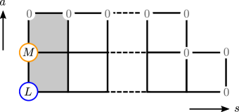
Figure 6.2: The Young tableaux associated to the rational $Q$-system. At each node of the Young diagram we have one $Q$-function denoted by $Q_{a,s}$. The number in each circle denotes the power of the polynomial.

For the $\mathfrak{su}(2)$ spin chain with length $L$ and magnon number $M$, the Young tableaux has two rows with the number of boxes given by $(M,L-M)$, where $L-M\geq M$. At each node of the Young tableaux, we define a $Q$-function. The $Q$-functions satisfy the following $QQ$-relation

$$Q_{a+1,s}(u)Q_{a,s+1}(u)=Q_{a+1,s+1}^{-}(u)Q_{a,s}^{+}(u)-Q_{a+1,s+1}^{+}(u)Q_{a,s}^{-}(u)\,,$$ (6.27)

where we have introduced the notation $f^{\pm}(u)\equiv f(u\pm\frac{i}{2})$. We impose the boundary conditions $Q_{a,s}=1$ at the upper-right boundary, together with $Q_{0,0}(u)=u^{L}$. One can then parameterize the $Q_{1,0}$ by

$$Q_{1,0}(u)=\prod_{j=1}^{M}(u-u_{j})=u^{M}+\sum_{k=0}^{M-1}c_{k}u^{k}.$$ (6.28)

Requiring all the $Q_{a,s}$ functions on the Young tableaux to be polynomials, we obtain a set of equations for the coefficients $\{c_{k}\}$ in (6.28), which can be solved analytically or numerically. The zeros of $Q_{1,0}(u)$ then give the corresponding Bethe roots.

A comment is in order here. The $QQ$-relations (6.27) are in fact defined by proportionality. This means the $QQ$-relation

$$Q_{a+1,s}(u)Q_{a,s+1}(u)={\kappa_{a}}\left(Q_{a+1,s+1}^{+}(u)Q_{a,s}^{-}(u)-Q_{a+1,s+1}^{-}(u)Q_{a,s}^{+}(u)\right)\,,$$ (6.29)

is equivalent to (6.27) in the sense that they lead to the same Bethe roots.

Now we turn to the twisted spin chain. To incorporate the twist in the rational $Q$-system, we modify the $QQ$-relation [33] as follows

$$Q_{a+1,s}(u)Q_{a,s+1}(u)={\kappa_{a}}\,Q_{a+1,s+1}^{-}(u)Q_{a,s}^{+}(u)-Q_{a+1,s+1}^{+}(u)Q_{a,s}^{-}(u)\,,$$ (6.30)

where $\kappa_{a}$ are $u$ independent constants. Notice that we multiply different factors onto the two terms on the right-hand side. We will call this deformed $QQ$-relation (6.30) the $\kappa QQ$-relation.

The $\kappa QQ$-relation can be defined for the $\mathfrak{su}(N)$ spin chain and provides a method to solve the corresponding twisted Bethe equations. For our purpose, we consider only the $\mathfrak{su}(2)$ case where the Young tableaux have two rows. We impose the same boundary conditions $Q_{2,s}=1$ at the upper-right boundary, and $Q_{0,0}(u)=u^{L}$ in the lower-left corner. For this simple situation, the $\kappa QQ$ relations can be solved explicitly as follows.

First, consider the $\kappa QQ$ relation for $a=1$. By taking into account the boundary condition we find

$$Q_{1,s+1}(u)=\kappa_{1}\,Q_{1,s}^{+}(u)-Q_{1,s}^{-}(u)\,.$$ (6.31)

This is a finite-difference equation whose solution is given by [31, 32]

$$Q_{1,n}(u)=Q^{(n)}_{\kappa_{1}}(u)\equiv\widetilde{D}^{n}_{\kappa_{1}}Q(u)\,,$$ (6.32)

where the twisted discrete derivative is defined by

$$\widetilde{D}_{\kappa}f(u)={\kappa}f(u+\tfrac{i}{2})-f(u-\tfrac{i}{2})\,.$$ (6.33)

Taking then $a=0$ in the $\kappa QQ$-relation, we obtain

$$Q_{0,n}=\frac{{\kappa_{0}}\,Q^{(n)-}_{\kappa_{1}}Q_{0,s}^{+}-Q^{(n)+}_{\kappa_{1}}Q_{0,s}^{-}}{Q^{(n-1)}_{\kappa_{1}}}\,.$$ (6.34)

Bethe equations.

Let us derive the Bethe equations from the $\kappa QQ$-relations. Consider the following $\kappa QQ$-relations

$$Q_{1,1}(u)= \,\kappa_{1}\,Q_{1,0}^{+}(u)-Q_{1,0}^{-}(u)\,,$$ (6.35a)

$$Q_{1,0}(u)Q_{0,1}(u)= \,\kappa_{0}\,Q_{1,1}^{-}(u)Q_{0,0}^{+}(u)-Q_{1,1}^{+}(u)Q_{0,0}^{-}(u)\,.$$ (6.35b)

The Bethe equations can be derived by requiring that all the $Q_{a,s}$ be polynomials in $u$. As for the non-twisted case, the zeros of $Q_{1,0}(u)$ are the Bethe roots, which we will denote by $\{u_{k}\}$. We evaluate the equations (6.35) at one of the Bethe roots $u_{k}$. From (6.35a) we obtain

$$Q_{1,1}^{+}(u_{k})=\kappa_{1}\,Q_{1,0}^{++}(u_{k})\,,\qquad Q_{1,1}^{-}(u_{k})=-Q_{1,0}^{--}(u_{k})\,,$$ (6.36)

where the double signs mean double shifts, $f^{\pm\pm}(u)\equiv f(u\pm i)$. From (6.35b) we have

$$\kappa_{0}\,Q_{1,1}^{-}(u_{k})Q_{0,0}^{+}(u_{k})-Q_{1,1}^{+}(u_{k})Q_{0,0}^{-}(u_{k})=0\,.$$ (6.37)

Combining these two equations, we find that

$$\kappa_{0}Q_{1,0}^{--}(u_{k})Q_{0,0}^{+}(u_{k})+\kappa_{1}Q_{1,0}^{++}(u_{k})Q_{0,0}^{-}(u_{k})=0\,.$$ (6.38)

Using the fact that

$$Q_{0,0}(u)=u^{L},\qquad Q_{1,0}(u)=\prod_{j=1}^{M}(u-u_{j})\,,$$ (6.39)

we see that (6.38) is precisely the twisted Bethe equation

$$-\frac{\kappa_{1}}{\kappa_{0}}=\left(\frac{u_{k}+\tfrac{i}{2}}{u_{k}-\tfrac{i}{2}}\right)^{L}\prod_{j=1}^{M}\frac{u_{k}-u_{j}-i}{u_{k}-u_{j}+i}\,.$$ (6.40)

Similar to the untwisted case, the requirement that all $Q_{a,s}$ be polynomials in $u$ leads to a set of algebraic equations—the zero-remainder conditions (ZRC)—for the coefficients of the $Q$-functions. In our case, the ZRC now depend on the twists. The ZRC for fixed values of $\kappa_{0}$ and $\kappa_{1}$ can be solved numerically. We find that for the system with length $L$ and magnon number $M$, the number of solutions for non-trivial twist is $L\choose M$. We have checked numerically that the solutions of the $\kappa QQ$-relation indeed solve the twisted Bethe equation.

6.3 Twisted $Q$-system of the XXZ spin chain

We are now ready to generalize the $\kappa QQ$-relation to the $q$-deformed case, for which the XXX chain just considered is the special case $q=1$. We consider the multiplicative variable $t=e^{u}$ as in (6.22). The $\kappa QQ$-relation takes the same form

$$Q_{a+1,s}(t)Q_{a,s+1}(t)={\kappa_{a}}\,Q_{a+1,s+1}^{-}(t)Q_{a,s}^{+}(t)-Q_{a+1,s+1}^{+}(u)Q_{a,s}^{-}(t)\,,$$ (6.41)

where now $f^{\pm}(t)\equiv f(tq^{\pm 1/2})$, and we have introduced twist parameters $\kappa_{0}$ and $\kappa_{1}$. We focus on the $U_{q}(sl(2))$ case where the corresponding Young tableaux has two rows. The boundary conditions are

$$Q_{0,0}(t)=(t-t^{-1})^{L}\,,\qquad Q_{1,0}(t)=Q(t)=\prod_{j=1}^{M}(tt_{j}^{-1}-t^{-1}t_{j})\,.$$ (6.42)

Both $Q$-functions are Laurent polynomials in $t$. The twisted discrete derivative in the $q$-deformed case is defined by

$$\widetilde{D}_{q,\kappa}f(t)={\kappa}\,f(tq^{+1/2})-f(tq^{-1/2})\,.$$ (6.43)

Again we can solve the $\kappa QQ$-relation explicitly, and find that $Q_{1,n}(t)=Q^{(n)}(t)=\widetilde{D}^{n}_{q,\kappa_{1}}Q(t)$. Similarly, $Q_{0,n}(t)$ is given by

$$Q_{0,n}(t)=\frac{{\kappa_{0}}\,Q^{(n)+}Q_{0,n-1}^{-}-Q^{(n)-}Q_{0,n-1}^{+}}{Q^{(n-1)}}\,.$$ (6.44)

By requiring all $Q_{0,n}(t)$ to be polynomials in $t$ and $t^{-1}$, we obtain a set of zero-remainder conditions. Going through the same steps as the XXX case, we find

$$\left(\frac{t_{j}^{2}\,q-1}{t_{j}^{2}-q}\right)^{L}=-\frac{\kappa_{1}}{\kappa_{0}}\prod_{k=1}^{M}\frac{t_{j}^{2}\,q^{2}-t_{k}^{2}}{t_{j}^{2}-t_{k}^{2}\,q^{2}}\,.$$ (6.45)

By identifying $\kappa_{1}=\kappa^{-}$ and $\kappa_{0}=\kappa^{+}$, we reproduce the Bethe equation of the twisted XXZ spin chain (6.23). For generic $q$ and $\kappa^{\pm}$, the ZRCs can be solved numerically. We have checked that for length $L$ and magnon number $M$, the number of solutions of the ZRC is ${L\choose M}$ and they give the correct Bethe roots. The situation where $q$ is a root of unity is also interesting, but more subtle, and it will be analyzed elsewhere.

6.4 An explicit example

In order to illustrate that we can reproduce the result for the loop model from the twisted XXZ spin chain, we consider the example with $L=2$ in this subsection. In aTL language, there are two standard modules with $j=0,1$, which correspond to the two sectors of the XXZ spin chain with magnon numbers $M=1,0$ respectively. From now on, we take the twists to be $\kappa^{\pm}=\rho^{\pm 1}$.

• $j=1$. This corresponds to the sector $M=0$. We have $Q(t)=1$ and the transfer matrix (6.24) reads

  $$t_{1,\rho}(t)=\rho\,\left(\frac{t^{2}q-1}{t^{2}-q}\right)^{2}+\rho^{-1}\,.$$ (6.46)

  The transfer matrix of the loop model is given by fixing the spectral parameter to a special value $t^{2}=-1$. Plugging this into (6.46), we obtain

  $$t_{1,\rho}\equiv t_{1,\rho}(i)=\rho+\rho^{-1}\,,$$ (6.47)

  in agreement with (4.9).

• $j=0$. This corresponds to the sector $M=1$. We evaluate the transfer matrix at $t=i$,

  $$t_{0}(i)=\rho\frac{Q(iq^{-1})}{Q(i)}+\rho^{-1}\frac{Q(iq)}{Q(i)}\,.$$ (6.48)

  The $Q$-function is given by

  $$Q(t)=t+\frac{1}{c_{0}t}\,,$$ (6.49)

  where $c_{0}$ satisfies the ZRC

  $$(q^{2}-\rho^{2})c_{0}^{2}+2q(1-\rho^{2})c_{0}+(1-q^{2}\rho^{2})=0\,.$$ (6.50)

  Assuming for the moment $q^{2}-\rho^{2}\neq 0$, we have two solutions for $c_{0}$:

  $$c_{0}^{(1)}=-\frac{q\rho+1}{\rho+q}\,,\qquad c_{0}^{(2)}=-\frac{q\rho-1}{\rho-q}\,.$$ (6.51)

  Plugging into the transfer matrix (6.48), the corresponding two eigenvalues are

  $$t_{0}^{(1)}=-2+(q+q^{-1})+(\rho+\rho^{-1})\,,\qquad t_{0}^{(2)}=2-(q+q^{-1})+(\rho+\rho^{-1})\,.$$ (6.52)

  Now taking $\rho=-q$, we obtain

  $$t_{0}^{(1)}=-2\,,\qquad t_{0}^{(2)}=2+2\mathfrak{m}\,,$$ (6.53)

  in accord with (4.8), where $\mathfrak{m}$ is defined in (2.10). We see that (6.53) gives precisely the two eigenvalues of the transfer matrix of the aTL loop model.

Before ending the section, let us make a comment here. We find that in the ZRCs (6.50), the case $\rho=\pm q$ is special. In this case, the quadratic equation becomes a linear equation and the number of solutions is reduced from 2 to 1. As we will explain in more detail in the next section, this is a general phenomenon. When $\rho$ and $q$ satisfy certain relations, the number of solutions of the ZRC changes. These relations, as we shall see, are precisely the resonance conditions of the standard module.

7 Resonance condition from algebraic geometry

As we have seen in section 2, for generic values of $q$ and $\rho$, the standard module $\mathcal{W}_{j,\rho^{2}}$ is irreducible with dimension $\hat{d}_{j}$. However, when $\rho$ satisfies the resonance condition, the representation becomes reducible and we can define the quotient module. From the Bethe ansatz perspective, the dimension of the standard module corresponds to the number of physical solutions of the Bethe equations. We therefore expect the structure of solutions to change at these special values of $\rho$. One simple example has been given in the previous section.

How can we see such a change in the number of solutions? One approach is by using the Gröbner basis. For a given set of algebraic equations, which are the ZRCs in our context, we can compute the Gröbner basis by following the standard algorithm. The number of solutions is given by the dimension of the quotient ring, whose basis is characterized by the leading terms of the Gröbner basis. Therefore, we expect that at special values, some coefficients of the leading terms of the Gröbner basis vanish.

To test this expectation, we consider three explicit examples, $(L,M)=(4,1),(4,2)$ and $(L,M)=(6,3)$, in what follows. We will take a careful look at the leading terms of the Gröbner basis. At special value of the twists, some leading terms of the Gröbner basis vanish and the dimension of the quotient ring changes.

7.1 Example 1: $L=4$, $M=1$

For $L=4$, $M=1$, the $Q_{1,0}(t)$ is given by

$$Q_{1,0}(t)=t+\frac{1}{c_{0}t}\,.$$ (7.1)

The rational $Q$-system leads to the following ZRC

$$0= \,(\rho^{2}-q^{4})(q^{2}-1){\color[rgb]{0,0,1}c_{0}^{4}}+4q(\rho^{2}-q^{2})(q^{2}-1){\color[rgb]{0,0,1}c_{0}^{3}}+6q^{2}(q^{2}-1)(\rho^{2}-1){\color[rgb]{0,0,1}c_{0}^{2}}$$ (7.2)

$$\,+4q(\rho^{2}q^{2}-1)(q^{2}-1){\color[rgb]{0,0,1}c_{0}}+(\rho^{2}q^{4}-1)(q^{2}-1)\,.$$

This is a single-variable polynomial equation. Note that for $q=\pm 1$, the right-hand side is zero identically, which implies that there are infinitely many solutions to the ZRC in this case. This is nothing but a manifestation of the subtleties at $q$ being a root of unity. Here we focus on generic $q$, therefore we can strip off the global factor $q^{2}-1$. The Gröbner basis can be computed straightforwardly and is given by

$$g_{1}=(q^{4}-\rho^{2}){\color[rgb]{0,0,1}c_{0}^{4}}+4q(q^{2}-\rho^{2}){\color[rgb]{0,0,1}c_{0}^{3}}-6q^{2}(\rho^{2}-1){\color[rgb]{0,0,1}c_{0}^{2}}+4q(1-q^{2}\rho^{2}){\color[rgb]{0,0,1}c_{0}}+(1-q^{4}\rho^{2})\,.$$ (7.3)

The leading term of the Gröbner basis is

$$\text{LT}[g_{1}]=(q^{4}-\rho^{2}){\color[rgb]{0,0,1}c_{0}^{4}}\,,$$ (7.4)

from which we can read off the quotient-ring basis

$$\{c_{0}^{3},c_{0}^{2},c_{0},1\}.$$ (7.5)

This implies that there are 4 physical solutions to the twisted Bethe equation with $L=4$, $M=1$.

Special twist.

It is easy to see that the leading term’s coefficient (7.4) vanishes at the specific values of the twist $\rho^{2}=q^{4}$. This hints that if we set $\rho=\pm q^{2}$, the number of solutions may be different from the generic case. Indeed, taking $\rho=q^{2}$, we find the following ZRC

$$0= \,4q^{3}(q^{2}-1)^{2}\,{\color[rgb]{0,0,1}c_{0}^{3}}+6q^{2}(q^{2}+1)(q^{2}-1)^{2}\,{\color[rgb]{0,0,1}c_{0}^{2}}$$ (7.6)

$$\,+4q(1-q^{2}-q^{6}+q^{8})\,{\color[rgb]{0,0,1}c_{0}}+(1-q^{2}-q^{8}+q^{10})\,.$$

The corresponding Gröbner basis is given by

$$g_{1}=4q^{3}\,{\color[rgb]{0,0,1}c_{0}^{3}}+6q^{2}(1+q^{2})\,{\color[rgb]{0,0,1}c_{0}^{2}}+4q(1+q^{2}+q^{4})\,{\color[rgb]{0,0,1}c_{0}}+(1+q^{2})(1+q^{4})\,.$$ (7.7)

The leading term is

$$\text{LT}[g_{1}]=4q^{3}\,{\color[rgb]{0,0,1}c_{0}^{3}}\,,$$ (7.8)

which leads to the quotient ring basis

$$\{c_{0}^{2},c_{0},1\}\,.$$ (7.9)

Therefore, we see that at $\rho=q^{2}$, the number of solution is 3.

Resonance condition.

Let us now compare what we have found with the resonance condition of the aTL representation discussed in section 7. At the special value $\rho=q^{2}$, the corresponding standard module $\mathcal{W}_{1,q^{2}}$ satisfies the resonance condition (2.18) with $(j,z)=(1,q^{2})$ and $(j^{\prime},z^{\prime})=(2,q)$. The quotient module is

$$\overline{\mathcal{W}}_{1,q^{2}}=\mathcal{W}_{1,q^{2}}/\mathcal{W}_{2,q}\,,$$ (7.10)

with the corresponding dimension

$$\bar{d}_{1}=\text{dim}\,\overline{\mathcal{W}}_{1,q^{2}}={4\choose 2+1}-{4\choose 2+2}=3\,.$$ (7.11)

This matches nicely with the dimension of the quotient ring (7.9).

7.2 Example 2: $L=4$, $M=2$

Now we consider a more complicated case with $L=4$, $M=2$. In this case, the $Q_{1,0}$ function is given by

$$Q_{1,0}(t)=t^{2}+c_{1}+\frac{1}{c_{0}\,t^{2}}\,.$$ (7.12)

The ZRC gives a set of algebraic equations for $\{c_{0},c_{1}\}$. These equations are too long to be presented here. The Gröbner basis of the ZRC in this case, with respect to degree-reverse lexicographic ordering, consists of four polynomials $\{g_{1},g_{2},g_{3},g_{4}\}$. The leading terms are given by

$$\text{LT}[g_{1}]=q^{2}(q^{2}\rho^{2}-1)^{3}\,{\color[rgb]{0,0,1}c_{1}^{3}}\,,$$ (7.13)

$$\text{LT}[g_{2}]=q^{2}(\rho^{2}-1)(q^{2}\rho^{2}-1)\,{\color[rgb]{0,0,1}c_{0}c_{1}^{2}}\,,$$

$$\text{LT}[g_{3}]=(q^{2}-\rho^{2})^{2}\,{\color[rgb]{0,0,1}c_{0}^{2}c_{1}}\,,$$

$$\text{LT}[g_{4}]=(q^{4}-\rho^{2})(q^{2}-\rho^{2})^{3}\,{\color[rgb]{0,0,1}c_{0}^{3}}\,,$$

where the blue-colored parts are the monomials in $c_{0}$ and $c_{1}$, and the rest are coefficients. At generic values of $\rho$ and $q$, the basis of the quotient ring is given by

$$\{c_{0}^{2},\,c_{1}^{2},\,c_{0}c_{1},\,c_{0},\,c_{1},\,1\}\,,$$ (7.14)

which implies that the corresponding twisted Bethe equations have 6 physical solutions.

Special twists and resonance conditions.

From (7.13), we see that one or more of the leading terms’ coefficients vanish when

$$\rho^{2}=1\,,\qquad\rho^{2}=q^{\pm 2}\,,\qquad\rho^{2}=q^{4}\,.$$ (7.15)

The case $\rho^{2}=1$ corresponds to the twist-less case. The other two cases, $\rho=q^{\pm 1},q^{\pm 2}$, correspond exactly to the two resonance conditions $(j,j^{\prime})=(0,1),(0,2)$ given in (2.18).

Since the coefficient vanish at the special points, they need to be treated separately. We can set $\rho$ to these special values in the $\kappa QQ$-relation, and then calculate the Gröbner basis. For $\rho=q$, the leading terms for the Gröbner basis now become

$$\text{LT}[g_{1}]=(q^{2}+1){\color[rgb]{0,0,1}c_{1}}\,,$$ (7.16)

$$\text{LT}[g_{2}]=q^{2}(q^{2}+4q+1)(q^{2}-4q+1){\color[rgb]{0,0,1}c_{0}^{2}}\,,$$

from which it is easy to see that the dimension of the quotient ring is 2. This matches the dimension of the quotient module given in (2.20) with $L=4$ and $(j,j^{\prime})=(0,1)$.

Taking instead $\rho=q^{2}$, the leading terms of the Gröbner basis become

$$\text{LT}[g_{1}]=6q^{6}\,{\color[rgb]{0,0,1}c_{0}^{2}}\,,$$ (7.17)

$$\text{LT}[g_{2}]=(q^{2}-q+1)^{3}(q^{2}+q+1)^{3}\,{\color[rgb]{0,0,1}c_{1}^{3}}\,,$$

$$\text{LT}[g_{3}]=(q^{2}-q+1)(q^{2}+q+1)\,{\color[rgb]{0,0,1}c_{0}c_{1}^{2}}\,,$$

from which we find that the dimension of the quotient ring is now 5. This matches the dimension of the quotient module given in (2.20) with $L=4$ and $(j,j^{\prime})=(0,2)$.

7.3 Example 3: $L=6$, $M=3$

In this case, the $Q_{1,0}$ function reads

$$Q_{1,0}(t)=t^{3}+c_{2}\,t+\frac{c_{1}}{t}+\frac{1}{c_{0}t^{3}}\,.$$ (7.18)

The ZRC leads to a set of algebraic equations in $\{c_{0},c_{1},c_{2}\}$. The corresponding Gröbner basis consists of 12 polynomials $\{g_{1},\ldots,g_{12}\}$. The leading terms are given by

$$\text{LT}[g_{1}]=(q^{2}-\rho^{2})(q^{4}-\rho^{2})\,{\color[rgb]{0,0,1}c_{0}^{2}c_{1}}\,,$$ (7.19)

$$\text{LT}[g_{2}]=q^{4}(q^{2}-\rho^{2})(q^{2}\rho^{2}-1)^{2}(q^{4}\rho^{2}-1)\,{\color[rgb]{0,0,1}c_{2}^{4}}\,,$$

$$\text{LT}[g_{3}]=q^{4}(q^{2}\rho^{2}-1)^{3}G_{1}(q,\rho)\,{\color[rgb]{0,0,1}c_{1}c_{2}^{3}}\,,$$

$$\text{LT}[g_{4}]=q^{4}(q^{2}-\rho^{2})(\rho^{2}-1)(q^{2}\rho^{2}-1)\,{\color[rgb]{0,0,1}c_{0}c_{2}^{3}}\,,$$

$$\text{LT}[g_{5}]=q^{6}(\rho^{2}-1)^{2}(q^{2}\rho^{2}-1)^{3}G_{2}(q,\rho)\,{\color[rgb]{0,0,1}c_{1}^{2}c_{2}^{2}}\,,$$

$$\text{LT}[g_{6}]=q^{4}(\rho^{2}-1)^{2}(q^{2}\rho^{2}-1)\,{\color[rgb]{0,0,1}c_{0}c_{1}c_{2}^{2}}\,,$$

$$\text{LT}[g_{7}]=q^{6}(\rho^{2}-1)^{2}(q^{4}-\rho^{2})(q^{2}\rho^{2}-1)^{4}(q^{4}\rho^{2}-1)^{2}G_{1}(q,\rho)G_{2}(q,\rho)\,{\color[rgb]{0,0,1}c_{1}^{3}c_{2}}\,,$$

$$\text{LT}[g_{8}]=q^{2}(\rho^{2}-1)(q^{2}-\rho^{2})(q^{4}-\rho^{2})(q^{2}\rho^{2}-1)^{2}\,{\color[rgb]{0,0,1}c_{0}c_{1}^{2}c_{2}}\,,$$

$$\text{LT}[g_{9}]=(q^{2}-\rho^{2})^{4}(q^{4}-\rho^{2})^{3}(q^{4}\rho^{2}-1)\,{\color[rgb]{0,0,1}c_{0}^{3}c_{2}}\,,$$

$$\text{LT}[g_{10}]=q^{4}(\rho^{2}-1)(q^{2}-\rho^{2})(q^{4}-\rho^{2})(q^{2}\rho^{2}-1)^{4}(q^{4}\rho^{2}-1)^{4}G_{1}(q,\rho)G_{2}(q,\rho)\,{\color[rgb]{0,0,1}c_{1}^{4}}\,,$$

$$\text{LT}[g_{11}]=q^{4}(\rho^{2}-1)(q^{2}-\rho^{2})^{2}(q^{4}-\rho^{2})(q^{2}\rho^{2}-1)^{2}(q^{4}\rho^{2}-1)\,{\color[rgb]{0,0,1}c_{0}c_{1}^{3}}\,,$$

$$\text{LT}[g_{12}]=(q^{2}-\rho^{2})^{4}(q^{4}-\rho^{2})^{4}(q^{6}-\rho^{2})(q^{4}\rho^{2}-1)G_{1}(q,\rho)G_{2}(q,\rho)\,{\color[rgb]{0,0,1}c_{0}^{4}}\,,$$

where the polynomials $G_{1}(q,\rho)$ and $G_{2}(q,\rho)$ are given by

$$G_{1}(q,\rho)= \,-2q^{6}\,\rho^{4}+(q^{8}+2q^{6}-2q^{4}+2q^{2}+1)\rho^{2}-2q^{2}\,,$$ (7.20)

$$G_{2}(q,\rho)= \,q^{6}\rho^{6}+(q^{10}-3q^{8}-2q^{6}+3q^{4}-q^{2}-1)\rho^{4}$$

$$+(q^{10}+q^{8}-3q^{6}+2q^{4}+3q^{2}-1)-q^{4}\,.$$

Special twists and resonance conditions.

We observe that there are several cases where the leading terms’ coefficient vanish. Firstly, $\rho^{2}=1$ corresponds to the twist-less case. Secondly we have the following conditions

$$\rho^{2}=q^{\pm 2}\,,\qquad\rho^{2}=q^{\pm 4}\,,\qquad\rho^{2}=q^{\pm 6}\,,$$ (7.21)

which correspond to the resonance conditions $(j,j^{\prime})=(0,1),(0,2),(0,3)$ in (2.18).

In this more complicated example, we also have the possibility that at certain values of $\rho$, the rather complicated polynomials $G_{1}(q,\rho)$ and $G_{2}(q,\rho)$ vanish. It is important to notice that the nature of these two types of special values of $\rho$ are different. By tuning $\rho$ to the special values $q^{\pm 1},q^{\pm 2},q^{\pm 3}$ which satisfy the resonance conditions (7.21) in the $\kappa QQ$-relation, we can verify that the dimensions of the resulting quotient rings are $5,14,19$ respectively. These are indeed the dimensions of the quotient modules.

On the other hand, we find numerically that if we take $\rho$ to be one of the values where $G_{1}(q,\rho)$ or $G_{2}(q,\rho)$ vanish, the dimension of the quotient ring does not change, and remains equal to 20. Let us take a more careful look at this point.

For generic value of $\rho$ and $q$, the corresponding quotient-ring basis is given by

$$\left\{c_{0}^{2}c_{2}^{2},c_{0}^{3},c_{0}c_{1}^{2},c_{1}^{3},c_{0}^{2}c_{2},c_{0}c_{1}c_{2},{\color[rgb]{1,0,0}c_{1}^{2}c_{2}},c_{0}c_{2}^{2},c_{1}c_{2}^{2},c_{2}^{3},c_{0}^{2},c_{0}c_{1},c_{1}^{2},c_{0}c_{2},c_{1}c_{2},c_{2}^{2},c_{0},c_{1},c_{2},1\right\}\,.$$ (7.22)

Now we consider the special value of $\rho$ such that $G_{1}(q,\rho)$ is vanishing. The leading-term monomials are then given by

$$\left\{c_{1}^{2}c_{2},c_{0}^{2}c_{1},c_{2}^{4},c_{0}c_{2}^{3},c_{0}c_{1}c_{2}^{2},c_{0}^{3}c_{2},c_{1}^{4},c_{0}c_{1}^{3},c_{0}^{4}\right\}\,.$$ (7.23)

We see that there are now only 9 polynomials in the Gröbner basis. Nevertheless, the quotient ring is still of dimension 20, with the following basis

$$\left\{c_{0}^{2}c_{2}^{2},{\color[rgb]{1,0,0}c_{1}c_{2}^{3}},c_{0}^{3},c_{0}c_{1}^{2},c_{1}^{3},c_{0}^{2}c_{2},c_{0}c_{1}c_{2},c_{0}c_{2}^{2},{c_{1}c_{2}^{2}},c_{2}^{3},c_{0}^{2},c_{0}c_{1},c_{1}^{2},c_{0}c_{2},c_{1}c_{2},c_{2}^{2},c_{0},c_{1},c_{2},1\right\}\,.$$ (7.24)

We find that the two quotient-ring bases are not exactly the same in (7.22) and (7.24). The difference stems from the red-colored monomials.

An alternative way to see the difference between the two types of special values of $\rho$ is by considering different orderings. For a different ordering, the Gröbner basis in general takes a different form. Nevertheless, at the special values which satisfy resonance conditions, the coefficients of the leading terms still vanish, such that the dimension of the quotient ring basis is different. On the other hand, for a differential ordering, the zeros of $G_{1}(q,\rho)$ and $G_{2}(q,\rho)$ in (7.20) in general no longer lead to vanishing leading terms of the new Gröbner basis. Therefore, these values are simply artifacts of the specific ordering that we choose.

7.4 General comments

From the above three examples, and by exploring more examples, we can make the following observations:

1. The resonance conditions of the aTL algebra can be obtained by requiring the coefficients of the leading terms of the Gröbner basis to vanish.

2. There are additional values of $\rho$ at which some of the leading terms’ coefficients vanish. Such additional values are artifacts of the specific basis we are working with. By choosing a different monominal ordering, they do not lead to vanishing coefficients anymore. Thus these values do not reflect the intrinsic properties of the equations themselves.

3. We can set the values of $\rho$ to satisfy the resonance condition in the $\kappa QQ$-relation. The number of solutions for such $\kappa QQ$-relation is precisely the dimension of the quotient module. We can compute the transfer matrices of the quotient module using these $\kappa QQ$-relations. There is then agreement between the dimension of the quotient ring and the dimension of the quotient module (2.19).

We emphasize that these are observations based on explicit examples and guided by physical intuitions. It would be very interesting to provide a more rigorous and general proof for these observations.

8 Algebraic-geometry approach to the torus partition function

In this section, we present the algebraic-geometry approach to computing the torus partition function of the loop model and the Potts model. Using this approach, we obtain closed-form expressions for the partition function $Z(L,N)$ for $L=4,6$ and arbitrary integer $N$, which will be presented in section 9. For larger $L$, we can compute the partition function for fixed $L$ up to 10 and for large $N$. The latter results are too long to be presented in the paper. Instead, for such cases we give the zeros of the partition functions. The zeros condense on certain curves in the $N\to\infty$ limit. Such condensation curves can be generated by numerical methods and perfectly match our results. This will be discussed in section 10.

8.1 General strategy

The main quantities to be computed are the companion matrices of the eigenvalues of the transfer matrices. For the chain on $L$ sites, the possible values of $j$ are $j=0,1,\ldots,\tfrac{L}{2}$. For the loop model, the value $j$ is the number of through-lines. It is related to the XXZ spin chain magnon numbers by $j=\tfrac{L}{2}-M$.

For each fixed $L$ and $j\neq 0$, the values of the twists are given by $\rho^{2}=\omega_{k}$ (4.4). We denote the companion matrix of the sector $j$ with the twist $\rho^{2}=\omega_{k}$ by $\mathbf{T}_{j,\omega_{k}}$.

The case $j=0$ is special. For $j=0$, the twist is given by $\rho^{2}=q^{2}$, which satisfies the resonance condition. This implies that the corresponding standard module $\mathcal{W}_{0,q^{2}}$ is reducible and we have $\overline{\mathcal{W}}_{0,q^{2}}=\mathcal{W}_{0,q^{2}}/\mathcal{W}_{1,1}$. Therefore, to compute the companion matrices of the transfer matrix, we can perform the computation over $\overline{\mathcal{W}}_{0,q^{2}}$ and $\mathcal{W}_{1,1}$ separately and then take the direct sum. More precisely, we denote the companion matrix of the transfer matrix over $\overline{\mathcal{W}}_{0,q^{2}}$ by $\overline{\mathbf{T}}_{0,q^{2}}$. We then have

$$\mathbf{T}_{0,q^{2}}=\overline{\mathbf{T}}_{0,q^{2}}\oplus\mathbf{T}_{1,1}.$$ (8.1)

As discussed in the previous section, the quotient ring of the ZRC which corresponds to $\overline{\mathcal{W}}_{0,q^{2}}$ is constructed by taking $\rho^{2}=q^{2}$ in the ZRC and then performing the standard algebraic-geometry computation.

Momentum decomposition.

The computation of the companion matrix can be simplified further by decomposing the quotient ring. In the current context, one natural way proceeds by performing a decomposition by the total lattice momentum of the spin chain. This method has been applied previously to the XXX spin chain [4]. The momentum decomposition for the twisted spin chain can be obtained as follows. The Bethe equations (6.17) can be written as

$$e^{ip(u_{l})L}=-\rho^{-2}\prod_{k=1}^{M}\frac{\sinh(u_{l}-u_{k}+\eta)}{\sinh(u_{l}-u_{k}-\eta)}\,,\qquad l=1,2,\ldots,M\,,$$ (8.2)

where $p(u_{l})$ is the momentum of each magnon. Taking the product of (8.2) for all $l$, we obtain

$$e^{iP_{M}L}=\rho^{-2M}\,,$$ (8.3)

where $P_{M}$ is the total momentum

$$P_{M}=p(u_{1})+p(u_{2})+\cdots+p(u_{M})\,.$$ (8.4)

Therefore we find that

$$e^{iP_{M}}=e^{\frac{2\pi in}{L}}\rho^{-\frac{2M}{L}}\,,\qquad n=1,2,\ldots,L\,.$$ (8.5)

On the other hand, we have

$$e^{iP_{M}}=\prod_{j=1}^{M}\frac{\sinh(u_{l}+\tfrac{\eta}{2})}{\sinh(u_{l}-\tfrac{\eta}{2})}=\prod_{j=1}^{M}\frac{t_{l}^{2}q-1}{t_{l}^{2}-q}=\frac{Q(q^{-1/2})}{Q(q^{+1/2})}\,.$$ (8.6)

Therefore, the momentum-decomposition condition is given by

$$\frac{Q(q^{-1/2})}{Q(q^{+1/2})}=e^{\frac{2\pi in}{L}}\rho^{-\frac{2M}{L}}\,,\qquad n=1,2,\ldots\,.$$ (8.7)

Thus, for a given through-line number $j\neq 0$, we have two independent decompositions. Each sector in the double decomposition is labeled by two integers $(n,k)$ where $n=1,\ldots,L$ and $k=1,\ldots,j$.

8.2 $TQ$-relation of the twisted spin chain

If we apply (6.24) to compute the companion matrix of the transfer matrix, we need to take the inverse of the companion matrix of $Q(i)$; see for example (6.48). There are two drawbacks for this strategy: (1) It is time consuming to take the inverse of the companion matrix analytically, especially when the dimension of the matrix is large; (2) Sometimes the determinant of the companion matrix of $Q(i)$ vanishes, so the matrix does not have an inverse, even though the eigenvalues of the transfer matrix are perfectly well-defined.

To avoid these problems, we can use the $TQ$-relation to express the eigenvalues of the transfer matrix directly in terms $\{c_{k}\}$, which are the coefficients of $Q(t)$. The procedure is as follows. Consider the transfer matrix (with a different normalization) for generic spectral parameter $t$. We have the following $TQ$-relation

$$\tilde{\tau}(t)Q(t)=\rho(t^{2}q-1)^{L}\,Q(tq^{-1})+\rho^{-1}(t^{2}-q)^{L}Q(tq)\,.$$ (8.8)

The eigenvalue of the transfer matrix $\tilde{\tau}(t)$ is a polynomial in $t$,

$$\tilde{\tau}(t)=\sum_{k=0}^{L}a_{k}\,t^{2k}\,.$$ (8.9)

Plugging this and (6.25) into the $TQ$-relation (8.8), and comparing the coefficients of different powers in $t$, we obtain a set of algebraic equations in $\{a_{k}\}$ and $\{c_{k}\}$. This set of equations are linear both in $\{a_{k}\}$ and $\{c_{k}\}$ and can be solved straightforwardly for $\{a_{k}\}$ in terms of $\{c_{k}\}$. Plugging back into (8.9), we can write $\tilde{\tau}(t)$ in terms of $\{c_{k}\}$. Once this is done, the transfer matrices that we need for the computation of the torus partition functions are given by

$$\tau_{M}=\frac{\tilde{\tau}(i)}{(-q-1)^{L}}\,.$$ (8.10)

The algebraic-geometry computation gives the companion matrix of $\{c_{k}\}$. Using the $TQ$-relation as described above, we obtain the companion matrix of $\tau_{M}$, which is the $\mathbf{T}_{j,\omega_{k}}$ we are after.

Compared to the transfer matrices appearing in (4.5), which are constructed using the link-pattern basis for the standard module, our companion matrix $\mathbf{T}_{j,\omega_{k}}$ takes a different form, but it share the same eigenvalues, viz., the matrices are related by a similarity transformation. Therefore we have

$$\text{tr}_{\mathcal{W}_{j,\rho^{2}=\omega_{k}}}\left[t\left(\frac{\gamma}{2}\right)^{N}\right]=\text{tr}\,\mathbf{T}_{j,\omega_{k}}^{N}$$ (8.11)

for any $N$.

8.3 The full partition function

In order to compute the torus partition function, we need to take the Markov trace of the transfer matrices. This is done just as before. Therefore the torus partition function can be computed as in (4.5),

$$Z_{\text{loop}}(L,N)=\text{tr}\,\mathbf{T}_{0,q^{2}}^{N}+\sum_{j=1}^{L/2}\sum_{m|j}\Lambda_{j,m}\sum_{k\in\kappa_{j}(m)}\text{tr}\,\mathbf{T}_{j,\omega_{k}}^{N}\,.$$ (8.12)

The same ingredients can be used to compute the torus partition function of Potts model,

$$Z_{\text{Potts}}(L,N)=\mathfrak{m}^{LN/2}\left\{\text{tr}\,\mathbf{T}_{0,q^{2}}^{N}+\frac{Q-1}{2}\text{tr}\,{\mathbf{T}_{0,-1}^{N}}+\sum_{j=1}^{L/2}\sum_{m|j}\widetilde{\Lambda}_{j,m}\sum_{k\in\kappa_{j}(m)}\text{tr}\,\mathbf{T}_{j,\omega_{k}}^{N}\right\}\,,$$ (8.13)

where $\widetilde{\Lambda}_{j,m}$ has been defined in (5.5).

Before presenting the explicit results, let us make a comment on the computational procedure. In principle, we can follow the standard algorithm and compute the Gröbner basis and companion matrices with generic parameters $\rho$ and $q$. In practice, however, keeping $\rho$ and $q$ generic slows down the computation considerably because bulky analytic expressions are generated in the intermediate steps. Therefore, we employ a slightly different strategy in the actual computation. The basic idea is to compute the results for different sets of values of $(\rho,q)$ and then interpolate the final result using this data. We refer to Appendix A for details.

9 Analytical results in closed form

In this section, we present the exact closed-form results for $L=4,6$ and general $N$.

9.1 Analytic result for the loop model

The analytic result for $L=4$ has been given in (4.18). This case is rather simple and we do not need to perform the decomposition to find the eigenvalues of the transfer matrix, although it makes the computation slightly more efficient. Using the algebraic-geometry approach, we reproduced the closed-form partition function (4.18), which we will not repeat here.

Let us now consider the $L=6$ case. The partition function is given by

$$Z_{\text{Loop}}(6,N)= \,\text{tr}\,\mathbf{T}_{0,q^{2}}^{N}+\Lambda_{1,1}\,\text{tr}\,\mathbf{T}_{1,1}^{N}+\Lambda_{2,1}\,\text{tr}\,\mathbf{T}_{2,1}^{N}+\Lambda_{2,2}\,\text{tr}\,\mathbf{T}_{2,-1}^{N}$$ (9.1)

$$\,+\Lambda_{3,1}\,\text{tr}\,\mathbf{T}_{3,1}^{N}+\Lambda_{3,3}\left[\mathbf{T}_{3,e^{2i\pi/3}}^{N}+\mathbf{T}_{3,e^{4i\pi/3}}^{N}\right]\,.$$

The multiplicities $\Lambda_{i,j}$ are given by

$$\Lambda_{1,1}= \,\mathfrak{m}^{2}-2,$$ (9.2)

$$\Lambda_{2,1}= \,\frac{1}{2}\mathfrak{m}^{2}(\mathfrak{m}^{2}-3)\,,$$

$$\Lambda_{2,2}= \,\frac{1}{2}(\mathfrak{m}^{4}-5\mathfrak{m}^{2}+4)\,,$$

$$\Lambda_{3,1}= \,\frac{1}{3}(\mathfrak{m}^{6}-6\mathfrak{m}^{4}+11\mathfrak{m}^{2}-6)\,,$$

$$\Lambda_{3,3}= \,\frac{1}{3}\mathfrak{m}^{2}(\mathfrak{m}^{4}-6\mathfrak{m}^{2}+8)\,.$$

To obtain an analytic result, we need to find the eigenvalues of the companion matrices in the four sectors with $j=0,1,2,3$. The dimension of these companion matrices are $20,15,6,1$ respectively.

The $j=0$ case.

For $j=0$, there are no through-lines. We take the value of the twist to be $\rho=-q$. Such choice of the twist satisfies the resonance condition and we can compute the eigenvalues for the quotient module $\overline{\mathcal{W}}_{0,q^{2}}$ and the standard module $\mathcal{W}_{1,1}$.

The dimension of the quotient module $\overline{\mathcal{W}}_{0,q^{2}}$ is 5. The 5 eigenvalues of $\mathbf{T}_{0,q^{2}}$ are given by

$$\lambda_{0,-q}^{\text{quo}}(1)= \,-\mathfrak{m}^{2}+2\,,$$ (9.3)

$$\lambda_{0,-q}^{\text{quo}}(2)= \,-\mathfrak{m}^{2}+2\,,$$

$$\lambda_{0,-q}^{\text{quo}}(3)= \,-\mathfrak{m}^{3}-6\mathfrak{m}^{2}-8\mathfrak{m}-2\,,$$

$$\lambda_{0,-q}^{\text{quo}}(4)= \,\frac{1}{2}(\mathfrak{m}^{3}+8\mathfrak{m}^{2}+28\mathfrak{m}+28)-\frac{1}{2}(\mathfrak{m}+2)^{2}\sqrt{\mathfrak{m}^{2}+48}\,,$$

$$\lambda_{0,-q}^{\text{quo}}(5)= \,\frac{1}{2}(\mathfrak{m}^{3}+8\mathfrak{m}^{2}+28\mathfrak{m}+28)+\frac{1}{2}(\mathfrak{m}+2)^{2}\sqrt{\mathfrak{m}^{2}+48}\,.$$

The dimension of the standard module $\mathcal{W}_{1,1}$ is 15. To find the eigenvalues $\mathbf{T}_{1,1}$ analytically, we perform the momentum decomposition. The value of the twist is taken to be $\rho=-1$. We can take the momentum quantum number to be $p=1,2,\ldots,6$ for non-singular solutions $\mathrm{Q}_{M}(q^{1/2})\neq 0$, together with the singular case $\mathrm{Q}_{M}(q^{1/2})=\mathrm{Q}_{M}(q^{-1/2})=0$. We denote the eigenvalues in each sector by $\lambda_{0,-q}^{\text{std},p}(j)$ and $\lambda_{0,-q}^{\text{std},\text{s}}(j)$. We list the eigenvalues in each sector in what follows.

• $p=1$. There are 2 eigenvalues:

  $$\lambda_{0,-q}^{\text{std},1}(1)= \,-\frac{1}{2}(\mathfrak{m}^{2}+4\mathfrak{m}+8)+\frac{1}{2}(\mathfrak{m}+2)\sqrt{\mathfrak{m}^{2}+12}\,,$$ (9.4)

  $$\lambda_{0,-q}^{\text{std},1}(2)= \,-\frac{1}{2}(\mathfrak{m}^{2}+4\mathfrak{m}+8)-\frac{1}{2}(\mathfrak{m}+2)\sqrt{\mathfrak{m}^{2}+12}\,.$$

• $p=2$. There are 3 eigenvalues. The explicit forms of the eigenvalues are somewhat bulky and we first give the characteristic equation

  $$x^{3}+(4\mathfrak{m}^{2}+20\mathfrak{m}+30)x^{2}$$ (9.5)

  $$+2(\mathfrak{m}^{4}+10\mathfrak{m}^{3}+30\mathfrak{m}^{2}+40\mathfrak{m}+30)x+4(\mathfrak{m}^{5}+5\mathfrak{m}^{4}+10\mathfrak{m}^{3}+10\mathfrak{m}^{2}+4\mathfrak{m}+2)=0\,.$$

  We can use the standard formula to find the solution of the cubic equation. The solutions are given by

  $$\lambda_{0,-q}^{\text{std},2}(k)=-\frac{1}{3}\left(b+\xi^{k}C^{\tfrac{1}{3}}+\frac{\Delta}{\xi^{k}C^{\tfrac{1}{3}}}\right),\qquad k=1,2,3$$ (9.6)

  where $\xi=(-1+i\sqrt{3})/2$, and

  $$b= \,4\mathfrak{m}^{2}+20\mathfrak{m}+30\,,$$ (9.7)

  $$\Delta= \,10(\mathfrak{m}+2)^{2}(\mathfrak{m}^{2}+6\mathfrak{m}+18)\,,$$

  $$C= \,2(\mathfrak{m}+2)^{3}(14\mathfrak{m}^{3}+153\mathfrak{m}^{2}+594\mathfrak{m}+1188)$$

  $$+6i\sqrt{3}(\mathfrak{m}+2)^{4}\sqrt{2\mathfrak{m}^{4}+9\mathfrak{m}^{2}+432}\,.$$

• $p=3$. There are 2 eigenvalues, which are the same as in the $p=1$ case.

• $p=4$. There are 3 eigenvalues. The characteristic equation is

  $$x^{3}-2(\mathfrak{m}^{2}+5\mathfrak{m}+3)x^{2}$$ (9.8)

  $$+(-\mathfrak{m}^{4}-\mathfrak{m}^{3}+6\mathfrak{m}^{2}-4\mathfrak{m}-12)x+\mathfrak{m}^{5}+2\mathfrak{m}^{4}-2\mathfrak{m}^{3}+4\mathfrak{m}^{2}+16\mathfrak{m}+8=0\,.$$

  The solutions are again given by

  $$\lambda_{0,-q}^{\text{std},4}(k)=-\frac{1}{3}\left(b+\xi^{k}C^{\tfrac{1}{3}}+\frac{\Delta}{\xi^{k}C^{\tfrac{1}{3}}}\right),\qquad k=1,2,3$$ (9.9)

  where now

  $$b= \,-2(\mathfrak{m}^{2}+5\mathfrak{m}+3)\,,$$ (9.10)

  $$\Delta= \,(\mathfrak{m}+2)^{2}(7\mathfrak{m}^{2}+15\mathfrak{m}+18)\,,$$

  $$C= \,-\frac{1}{2}(\mathfrak{m}+2)^{3}(34\mathfrak{m}^{3}+117\mathfrak{m}^{2}+216\mathfrak{m}+108)$$

  $$+\frac{3i\sqrt{3}}{2}(\mathfrak{m}+2)^{4}\sqrt{8\mathfrak{m}^{4}+9\mathfrak{m}^{2}+108}\,.$$

• $p=5$. There is 1 eigenvalue,

  $$\lambda_{0,-q}^{\text{std},5}(1)=2\mathfrak{m}^{2}+6\mathfrak{m}+2\,.$$ (9.11)

• $p=6$. There are 3 eigenvalues, which are the same as in the $p=4$ case.

• Singular solution. There is 1 eigenvalue which is given by

  $$\lambda_{0,-q}^{\text{std},\text{s}}=2\mathfrak{m}+2\,.$$ (9.12)

The $j=1$ case.

For $j=1$, we have 2 through-lines and we take the value of the twist to be $\rho=-1$. This gives precisely the module $\mathcal{W}_{1,1}$. The eigenvalues of $\mathbf{T}_{1,1}$ has already been discussed in the $j=0$ case.

The $j=2$ case.

For $j=2$, we have 4 through-lines and we need to consider two values of the twist: $\rho=1$ and $\rho=i$. The companion matrices $\mathbf{T}_{2,1}$ and $\mathbf{T}_{2,-1}$ are 6-dimensional. The corresponding eigenvalues are given by:

• Eigenvalues of $\mathbf{T}_{2,1}$:

  $$\{-\mathfrak{m},-\mathfrak{m},-\mathfrak{m},-\mathfrak{m},-\mathfrak{m},12+5\mathfrak{m}\}\,.$$ (9.13)

• Eigenvalues of $\mathbf{T}_{2,-1}$:

  $$\{\pm(\mathfrak{m}+2),\pm(2+\sqrt{3})(\mathfrak{m}+2),\pm(2-\sqrt{3})(\mathfrak{m}+2)\}\,.$$ (9.14)

The $j=3$ case.

For $j=3$, we have 6 through-lines. This case is trivial and for generic value of twist $\rho$, we have

$$\mathbf{T}_{3,\rho^{2}}=\rho+\rho^{-1}\,.$$ (9.15)

We need to take $\rho=e^{i\pi/3},e^{2i\pi/3},1$ and thus

$$\mathbf{T}_{3,1}=2\,,\qquad\mathbf{T}_{3,e^{2i\pi/3}}=1\,,\qquad\mathbf{T}_{3,e^{4i\pi/3}}=-1\,.$$ (9.16)

Plugging all the eigenvalues of the transfer matrices into (9.1) gives the analytic expression of the partition function $Z_{\text{loop}}(6,N)$ of the loop model for any $N$.

9.2 Analytic result for the Potts model

To construct the partition function for the Potts model we need an additional piece, which is $\mathbf{T}_{0,-1}$ in the $j=0$ sector. For $L=4,6$, the companion matrix $\mathbf{T}_{0,-1}$ has dimension 6 and 20, respectively. We can find the analytic eigenvalues of the transfer matrix for $L=4$, but not for $L=6$. Therefore, we will write down the analytic expression for $L=4$

$$\frac{Z_{\text{Potts}}(4,N)}{\mathfrak{m}^{2N}}=\text{tr}\,\mathbf{T}_{0,q^{2}}^{N}+\frac{\mathfrak{m}^{2}-1}{2}\text{tr}\,\mathbf{T}_{0,-1}^{N}+\tilde{\Lambda}_{1,1}\,\text{tr}\,\mathbf{T}_{1,1}^{N}+\tilde{\Lambda}_{2,1}\,\text{tr}\,\mathbf{T}_{2,1}^{N}+\tilde{\Lambda}_{2,2}\,\text{tr}\,\mathbf{T}_{2,-1}^{N}\,,$$ (9.17)

where we have

$$\tilde{\Lambda}_{1,1}=-1\,,\qquad\tilde{\Lambda}_{2,1}=\frac{1}{2}\mathfrak{m}^{2}(\mathfrak{m}^{2}-3)\,,\qquad\tilde{\Lambda}_{2,2}=\frac{1}{2}(\mathfrak{m}^{2}-2)(\mathfrak{m}^{2}-1)\,.$$ (9.18)

There are 6 eigenvalues of $\mathbf{T}_{0,-1}$, given by

$$\left\{0,0,\frac{1}{2}(\mathfrak{m}+2)\big{(}\mathfrak{m}+4\pm\sqrt{\mathfrak{m}^{2}+16}\big{)},-\frac{1}{2}(\mathfrak{m}+2)\big{(}\mathfrak{m}+4\pm\sqrt{\mathfrak{m}^{2}+16}\big{)}\right\}.$$ (9.19)

Assuming $N$ is even, we find that the contribution of $\mathbf{T}_{1,1}^{N}$ cancels the same contribution in $\mathbf{T}_{0,q^{2}}^{N}$ and we find finally

$$Z_{\text{Potts}}(4,N)= \,\mathfrak{m}^{2N}\left\{(\mathfrak{m}^{2}+7\mathfrak{m}+8)^{N}+(\mathfrak{m}^{2}+\mathfrak{m})^{N}+2^{N-1}\mathfrak{m}^{2}(\mathfrak{m}^{2}-3)\right.$$ (9.20)

$$\,\left.+(\mathfrak{m}^{2}-1)(\mathfrak{m}+2)^{N}\left[(\mathfrak{m}+4+\sqrt{\mathfrak{m}^{2}+16})^{N}+(\mathfrak{m}+4-\sqrt{\mathfrak{m}^{2}+16})^{N}\right]\right\}.$$

10 Zeros of partition functions

In this section we investigate the zeros of the partition function $Z(L,N)$ in the plane of complex $\mathfrak{m}$. For simplicity, we shall focus on the loop model, where we recall that $\mathfrak{m}$ is the weight given to each loop; we leave the Potts model aside for future work. We are particularly interested in the partial thermodynamic limit, where $L$ is fixed and finite, but $N\gg L$.

10.1 Condensation curves

A convenient tool for describing the partial thermodynamic limit is provided by the Beraha-Kahane-Weiss (BKW) theorem [34]. It states that in the limit $N/L\to\infty$ the partition function zeros condense on certain curves in the complex $\mathfrak{m}$-plane, henceforth called condensation curves.

Let $\{\Lambda_{i}(\mathfrak{m})\}$ with $i=1,2,\ldots$ denote the union of eigenvalues of all the transfer matrices that build up the torus partition function (4.5). As we have seen, they can be obtained by diagonalizing $t(\gamma/2)$ in any one of the standard modules entering (4.5). For a given $\mathfrak{m}$, we order these eigenvalues by norm, $|\Lambda_{1}(\mathfrak{m})|\geq|\Lambda_{2}(\mathfrak{m})|\geq\cdots$, and we say that $\Lambda_{i}(\mathfrak{m})$ is dominant at $\mathfrak{m}$ if no other eigenvalue has a strictly greater norm. The BKW theorem [34] then states that the condensation curves are given by the loci where there are (at least) two dominant eigenvalues, $|\Lambda_{1}(u)|=|\Lambda_{2}(u)|$.

We shall use a numerical technique for tracing out the condensation curves that has already been detailed in our previous paper [4]. It combines an efficient method for the numerically exact diagonalization of the sparse transfer matrices with a direct-search method that allows us to trace out the condensation curves. The sparse matrix decomposition follows directly from the writing (3.1) of $t(u)$ as a product of $R$-matrices. The geometrical action can then be inferred from (3.3), where we take a link-pattern basis for each standard module. To take into account the possibility that the dominant eigenvalues may come from sectors with different through-line numbers we actually diagonalize the direct sum of $t(u)$ over all standard modules entering (4.5).

10.2 Results

The results for the condensation curves with $L=6,8,10,12,14$ are shown in Figure 10.3. Notice that the curves are invariant under changing the sign of ${\rm Im}\,\mathfrak{m}$. The first three cases, $L=6,8,10$, are compared to the partition function zeros for a system of large aspect ratio ($N=1024$), obtained from the algebraic-geometry computations. The agreement is seen to be perfect, but it should be noticed that the density of zeros on the curves exhibits considerable variation.

Apart from this, the condensation curves display several noteworthy features. For any $L$ they go through the points $\mathfrak{m}=0$ and $\mathfrak{m}=-2$ exactly. There is a central bubble ${\cal B}_{1}$ containing those two points, a number of branches extending out towards infinity, and a “necklace” region with many bifurcations and small enclosed regions that appears to produce, as $L$ increases, a larger bubble ${\cal B}_{2}$ that surrounds ${\cal B}_{1}$.

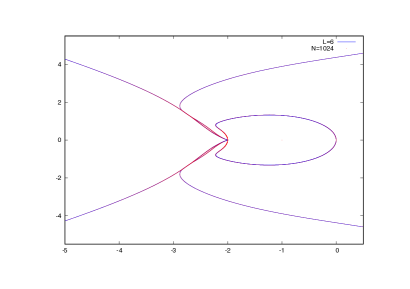
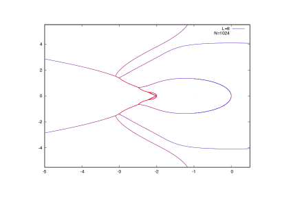
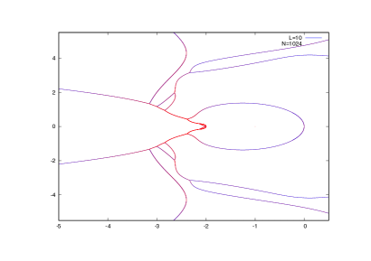
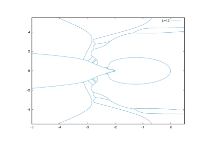
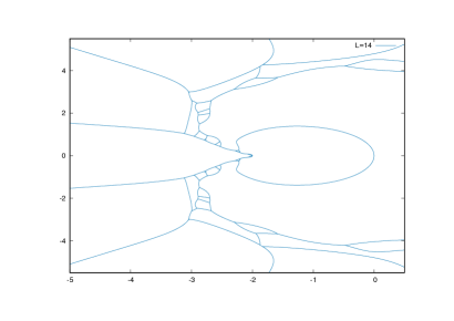
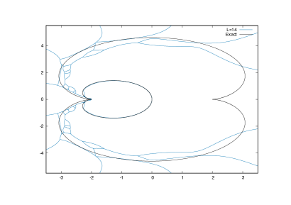
Figure 10.3: Condensation curves in the complex $\mathfrak{m}$-plane for partition-function zeros of the loop model on $L\times N$ tori, in the limit $N\to\infty$. The panels show, in reading direction, the cases $L=6,8,10,12,14$. The first three panels also superpose the partition-function zeros for a finite system with $N=1024$ (in red color). The last panel compares the $L=14$ curves with an exact prediction for the thermodynamic limit ($L\to\infty$).

We can provide the exact expressions of ${\cal B}_{1}$ and ${\cal B}_{2}$ in the thermodynamic limit ($L\to\infty$) by the following argument. The loop model is known to be critical along a segment of the real line, ${\cal S}=\{\mathfrak{m}|-2<\mathfrak{m}\leq 2\}$, and its continuum limit is described by the Coulomb Gas (CG) approach to conformal field theory [35]. It is natural to assume [36] that the model remains critical in a larger region ${\cal R}$ of the complex plane, with ${\cal S}\subset{\cal R}$, and that within ${\cal R}$ all the CG results remain valid by analytic continuation.

It is customary to parametrize the loop weight as

$$\mathfrak{m}=-2\cos(\pi g)\,,$$ (10.1)

where $g$ is called the CG coupling constant. Inside ${\cal S}$ we have $0<g\leq 1$. The critical exponents of the loop model are conveniently written in the Kac-table parametrization of conformal weights

$$h_{r,s}=\frac{(rg-s)^{2}-(g-1)^{2}}{4g}\,.$$ (10.2)

The model contains [35] in particular the identity operator $I$ of weight $h_{1,1}=0$, the energy operator $\varepsilon$ of weight $h_{3,1}$, and for any $j\in\mathbb{N}^{*}$ the $2j$-leg operators ${\cal O}_{j}$ of weight $h_{j,0}$. Notice that ${\cal O}_{j}$ is the dominant operator inside the standard module with $2j$ through-lines.

For $-2<\mathfrak{m}<0$, or $0<g<\frac{1}{2}$, we have that $h_{1,0}<0$, so the 2-leg operator is more relevant than the identity. Moreover, it is the operator of most negative conformal weight among the ${\cal O}_{j}$. The power-law behavior of correlation functions is governed by the real part of the conformal weights, so we can expect a phase transition to take place when ${\rm Re}\,h_{1,0}=0$. We hypothesize that the locus of this transition is precisely ${\cal B}_{1}$, in the thermodynamic limit. Since $h_{1,0}=\frac{1}{2}-\frac{1}{4g}$ by (10.2), we arrive at the prediction

$${\cal B}_{1}=-2\cos\left(\frac{\pi}{2+i\mathbb{R}}\right)\,.$$ (10.3)

This is in excellent agreement with the condensation curves, as witnessed by the comparison with the $L=14$ curve in the last panel of Figure 10.3.

The termination of critical behavior in the CG is related [35] to the fact that the energy operator $\varepsilon$, of weight $h_{3,1}=2g-1$, becomes marginal when $g\uparrow 1$ (i.e., $\mathfrak{m}\uparrow 2$). We therefore expect termination of critical behavior when ${\rm Re}\,h_{3,1}=1$. Hypothesizing that the locus of this transition is precisely ${\cal B}_{2}$ we arrive at our second prediction,

$${\cal B}_{2}=-2\cos\left(\frac{\pi}{1+i\mathbb{R}}\right)\,.$$ (10.4)

As seen from the last panel of Figure 10.3, this cuts right through the “necklace” region, and although finite-$L$ effects are definitely larger than in the case of ${\cal B}_{1}$, we expect this part of the condensation curves to converge to (10.4) when $L\to\infty$. We finally identify the region of criticality ${\cal R}$ with the interior of ${\cal B}_{2}$.

11 Conclusions and discussion

In this paper, we discovered a precise relation between representation theory of the aTL algebra and the algebraic structure of the solutions to the Bethe equations of the XXZ spin chain with a diagonal twist. While such a connection might seem surprising at the first glance, it turns out to be quite natural. One of the reasons that this connection appears to have been left unnoticed hitherto is presumably that it would be rather difficult to see it by solving the Bethe equation numerically. This demonstrates the power and usefulness of computational algebraic geometry in the study of integrable models.

Using this relation, we were able to compute the torus partition function of the O($\mathfrak{m}$) loop model and the $Q$-state Potts model in two very different ways, which we called the geometric algebra and algebraic geometry approaches, respectively. The final results of these two methods match nicely. We studied the distribution of partition-function zeros for $L=6,8,10$ in the partial thermodynamic limit and found that the zeros condense on certain curves. The condensation curves can be constructed directly in the partial thermodynamic limit and match beautifully with our numerical results of partition function zeros. We would like to highlight the fact that part of the condensation curves can be understood from conformal field theory in the full thermodynamic limit, $L\to\infty$. This is quite remarkable because usually condensation curves can only be determined numerically, while here we can write down the analytic formulae (10.3)–(10.4) for these curves.

As a byproduct of the algebraic-geometry approach, we constructed the rational $Q$-system for the twisted Bethe equations, both for the XXX and the XXZ spin chains. The main advantage of the rational $Q$-system, compared to the original Bethe equations, is that it leads to physical solutions only, and hence we do not need to impose further conditions to exclude unphysical ones. We expect that our construction generalizes naturally to higher-rank cases, some of which have recently been shown to harbor random-geometry applications generalizing those of the loop model [37, 38].

From the perspective of the CAG (Computational Algebraic Geometry)-BAE (Bethe Ansatz Equations) program, this work is the first step in applying CGA techniques to XXZ-type BAE, which are not polynomial equations in their original form, but which can nevertheless be rationalized by a proper change of variables. These equations contain free parameters, which are the anisotropic parameter $q$ and the twist $\rho^{2}$ in our case. On the one hand, these parameters bring richer structures to the equations because the solutions depend on the parameters. There can be special loci in the parameter space where the structure of the solutions change drastically and exhibit noteworthy features. The resonance condition which we analyzed in this paper is an example. On the other hand, it brings new challenges in the CAG computations. To start with, the zero-remainder conditions associated with the rational $Q$-system are more involved. At the same time, although the computation of Gröbner bases and companion matrices are purely algebraic and straightforward, the standard algorithm leads to rather bulky analytic expressions in intermediate steps. This fact slows down the computation considerably. This prohibits us from obtaining explicit analytic expression for $L>10$ by the algebraic-geometry approach.

A number of natural future directions can be pursued following the current work. One important immediate question is to investigate the case where $q$ is a root of unity. It has been known for a while that the representation theory of Temperley-Lieb algebra has an intricate structure [39] in this case. Already in the non-periodic case, this leads to indecomposable structures in the lattice model [40, 41] which entail strong connections to the corresponding structures in the logarithmic CFT that govern the continuum limit [42]. The case of periodic boundary conditions is even richer and, as yet, the resulting incomposable structures are only partially understood (see the review [43] and references therein). Given the relation established in the current paper for generic $q$, we expect that these structures should also be encoded in the solutions of the corresponding Bethe equations. Indeed, we can already see that all the Gröbner bases that we constructed in this paper exhibit vanishing leading coefficients when $q$ is an appropriate root of unity. Can we see more fine structures by using proper algebro-geometric tools? We leave this fascinating question for future studies.

Another natural generalization is to consider the XYZ spin chain. This case is even less investigated, as it is significantly more complicated. Following the strategy of the current paper, we need to seek for a proper change of variables to rationalize the Bethe equations which involve elliptic function. This seems to be possible following the treatment in [44], but with new features.

Apart from developing algebro-geometric methods for more general types of Bethe equations, one can also find applications of our method in broader contexts. So far we have mainly applied our methods to compute partition functions of important statistical-mechanical models, such as the six-vertex model [4] and the Potts model. In recent years, it has been discovered that integrable spin chains have deep connections with supersymmetric gauge theories in various setups. We give one potential application as an example. By the Bethe/gauge duality [45, 46, 47], Bethe-ansatz techniques can be applied to compute twisted superconformal indices [48]. The Bethe equations arising in this context are precisely those of the twisted XXZ spin chain which we studied in this paper. The algebraic-geometry approach developed here can be applied straightforwardly to compute twisted superconformal indices analytically.

Appendix A More on computational algebraic geometry

In this appendix, we provide an overview of the methods of computational algebraic geometry used in the main text. Our discussion contains two parts. In the first part, we introduce the basic notions of computational algebraic geometry with examples. Most of the contents in this part is standard. For more details we refer to the textbooks [49, 50]. When the algebraic equations under consideration contain extra free parameters, like the ZRC of the twisted XXZ spin chain, direct computations lead to rather complicated analytic expressions in the intermediate steps. This slows down the computations considerably. To improve the efficiency, we need to employ a slightly different strategy, which will be discussed in the second part.

A.1 Basic notions of computational algebraic geometry

Definition A.1

An affine algebraic set is the common zero set

$$V(f_{1},\ldots,f_{r})=\left\{p\in K^{n}\mid f_{1}(p)=0,\ldots,f_{r}(p)=0\right\}$$

of polynomials $f_{1},\ldots,f_{r}\in R=K[x_{1},\ldots,x_{n}]$.

Is there a structure in algebra which corresponds to the geometry? If $f_{1}\left(p\right)=0,\ldots,f_{s}\left(p\right)=0$ for $p\in K^{n}$, then also every $R$-linear combination of the $f_{i}$ vanishes on $p$, that is

$$\left(\sum_{i=1}^{s}r_{i}\cdot f_{i}\right)\left(p\right)=\sum_{i=1}^{s}r_{i}\left(p\right)f_{i}\left(p\right)=0$$

for all $r_{i}\in R$. This leads to a key concept in algebra, the notion of an ideal:

Definition A.2

Let $R$ be a commutative ring with $1$. An ideal is a non-empty subset $I\subset R$ with $a+b\in I$ and $ra\in I$ for all $a,b\in I$ and $r\in R$.

For $S\subset R$ we write $\left\langle S\right\rangle$ for the ideal generated by $S$, which consists of all finite $R$-linear combinations of elements of $S$.

So it makes sense to generalize our definition of a vanishing loci to arbitrary subsets $S\subset R$, and, as seen above, we have $V(f_{1},\ldots,f_{s})=V(\left\langle f_{1},\ldots,f_{s}\right\rangle)$. On the other hand, if $I\subset R$ is an ideal, then $V(I)$ is an algebraic set: Every ideal $I\subset R$ is finitely generated, that is, of the form $I=\left\langle f_{1},\ldots,f_{s}\right\rangle$ with $f_{i}\in R$. Rings with this property are called Noetherian.

Definition A.3

A commutative ring $S$ with $1$ is called Noetherian if every ideal $I\subset S$ is finitely generated, equivalently, if every ascending chain of ideals $I_{1}\subset I_{2}\subset\ldots$ becomes stationary.

Theorem A.4 (Hilbert Basis Theorem)

If $S$ is a Noetherian ring, then also $S\left[x\right]$ is Noetherian. In particular, if $K$ is a field then, by induction, $K\left[x_{1},\ldots,x_{n}\right]$ is Noetherian.

Definition A.5

Let $K$ be a field. An element

$$x^{\alpha}:=x_{1}^{\alpha_{1}}\cdot\ldots\cdot x_{n}^{\alpha_{n}}\in R$$

is called a monomial, and an element $c\cdot x^{\alpha}$ with $c\in K$ is called a term. Every polynomial $f\in R$ is a finite sum $f={\textstyle\sum\nolimits_{\alpha}}c_{\alpha}x^{\alpha}$ of terms. The degree $\deg(f)$ of $f$ is the maximal $\left|\alpha\right|:=\alpha_{1}+\ldots+\alpha_{n}$ with $c_{\alpha}\neq 0$.

If $>$ is a total ordering on the set of monomials of $R$ and $0\neq f\in R$, then the largest term $\operatorname{LT}(f)=c\cdot x^{\alpha}$ is called the lead term of $f$, $\operatorname{LC}(f)=c$ the lead coefficient of $f$, and $L(f)=x^{\alpha}$ the lead monomial of $f$. For $f=0$ we set $L(0)=LT(0)=LC(0)=0$.

Definition A.6

A monomial ordering on the semigroup of monomials $x^{\alpha}$ is a total ordering $>$ which respects multiplication, that is, $x^{\alpha}>x^{\beta}\Rightarrow x^{\alpha}x^{\gamma}>x^{\beta}x^{\gamma}$ for all $\alpha,\beta,\gamma$. A monomial ordering is global if it is a well ordering, equivalently if $x_{i}>1$ for all $i$.

Definition A.7

The most important global monomial orderings are the lexicographical ordering (lp), where $x^{\alpha}>x^{\beta}$ if the leftmost nonzero entry of $\alpha-\beta$ is positive, and the degree reverse ordering (dp), where we prefer the monomial of larger degree, and break a tie via $x^{\alpha}>x^{\beta}$ if there is an $1\leq i\leq n$ such that $\alpha_{n}=\beta_{n},\ldots,\alpha_{i+1}=\beta_{i+1},\alpha_{i}<\beta_{i}$. While the former is the key to solve multivariate polynomial systems, the latter usually leads to the best performance in computations.

Example A.8

Using $lp$ we divide $x^{2}y+x$ by $y-1$ and $x^{2}-1$:

$$\boldsymbol{x}^{2}\boldsymbol{y}+x=x^{2}\left(\boldsymbol{y}-1\right)+1\cdot\left(\boldsymbol{x}^{2}-1\right)+\underline{x+1}\text{.}$$

Here the lead terms are shown in bold and the remainder is underlined.

Definition A.9

Given a monomial ordering $>$ and a subset $G\subset R$, we define the leading ideal of $G$ as

$$L(G)=\left\langle L(f)\mid f\in G\backslash\{0\}\right\rangle\subset R\text{.}$$

Definition A.10 (Gröbner bases)

Given an ideal $I$ and a global monomial ordering $>$, then for a finite subset $G\subset I$ with $0\notin G$ obviously $L(G)\subset L(I)$, and we call $G$ a Gröbner basis of $I$ with respect to $>$, if $L(G)=L(I)$.

Theorem A.11

Every ideal $I\subset K[x_{1},\ldots,x_{n}]$ has a Gröbner basis.

Definition A.12

Given a set $G=\{g_{1},\ldots,g_{s}\}\subset R$, a normal form is a map $\operatorname*{NF}(-,G):R\rightarrow R$ with

1. $\operatorname*{NF}(0,G)=0$.

2. If $\operatorname*{NF}(f,G)\neq 0$ then $L(\operatorname*{NF}(f,G))\notin L(G)$.

3. For every $0\neq f\in R$ there are $a_{i}\in R$ with

   $$f-\operatorname*{NF}(f,G)={\textstyle\sum\nolimits_{i=1}^{s}}a_{i}g_{i}$$

   and $L(f)\geq L(a_{i}g_{i})$ for all $i$ with $a_{i}g_{i}\neq 0$. Such an expression we call a standard represenation of $f$.

Lemma A.13

Given a set $G=\{g_{1},\ldots,g_{s}\}\subset R$ and any order of preference of the $g_{i}$ in the division, the Buchberger division yields a normal form $\operatorname*{NF}(-,G)$, the Buchberger normal form.

Example A.14

If in Example A.8, we prefer the divisor $x^{2}-1$ over $y-1$, we obtain:

$$\boldsymbol{x^{2}y}+x=y\cdot\left(\boldsymbol{x^{2}}-1\right)+\underline{x+y}\ \$$

So depending on the choice made, the remainder will be $x+1$ or $x+y$.

Theorem A.15 (Ideal membership)

Let $I\subset R$ be an ideal and $f\in R$. If $G=\left\{g_{1},\ldots,g_{s}\right\}$ is a Gröbner basis of $I$ and $\operatorname*{NF}$ is a normal form, then

$$f\in I\Longleftrightarrow\operatorname*{NF}(f,G)=0\text{.}$$

Corollary A.16

If $G\$is a Gröbner basis of $I$, then $I=\left\langle G\right\rangle$.

Definition A.17

An element $f\in R$ is called reduced with respect to a set $G\subset R$, if no term of $f$ is contained in $L(G)$. A normal form $\operatorname*{NF}(-,G)$ is called a reduced normal form if $\operatorname*{NF}(f,G)$ is reduced with respect to $G$ for all $f$.

Example A.18

If we in the Buchberger normal form put non-divisible terms into the remainder also in intermediate steps, we obtain a reduced normal form, the reduced Buchberger normal form.

Example A.19

We can continue the Example A.14:

$$\boldsymbol{x}^{2}\boldsymbol{y}+x=y\cdot\left(\boldsymbol{x}^{2}-1\right)+\underline{x}+1\cdot(\boldsymbol{y}-1)+\underline{1}$$

Indeed, the remainder is now unique provided we divide by a Gröbner basis:

Theorem A.20

Let $>$ be a global ordering, $I\subset R$ an ideal, $f\in R$ and $G$ a Gröbner basis of $I$. If $\operatorname*{NF}(-,G)$ is a reduced normal form, then the map $\operatorname*{NF}(-,G)$ is uniquely determined by $>$ and $I$. We then also write $\operatorname*{NF}(-,I)$.

Remark A.21

Even when using a reduced normal form and a Gröbner basis, although the remainder is unique, the generated expression in the generators may not be. In the Examples A.8 and A.19 we obtain

$$\boldsymbol{x}^{2}\boldsymbol{y}+x=y\cdot\left(\boldsymbol{x}^{2}-1\right)+1\cdot(\boldsymbol{y}-1)+\underline{x+1}\vspace{-0.1cm}$$

and

$$\boldsymbol{x}^{2}\boldsymbol{y}+x=x^{2}\left(\boldsymbol{y}-1\right)+1\cdot\left(\boldsymbol{x}^{2}-1\right)+\underline{x+1}$$

respectively.

Gröbner bases can be computed via Buchberger’s algorithm, which is derived from

Theorem A.22 (Buchberger’s criterion)

If $I\subset R$ is an ideal, $\operatorname*{NF}$ a normal form and $0\notin G=\{g_{1},\ldots,g_{s}\}\subset I$, then $G$ is a Gröbner basis of $I$, if and only if $I=\left\langle G\right\rangle$ and $\operatorname*{NF}(\operatorname*{spoly}(g_{i},g_{j}),G)=0$ for all $i\neq j$, where

$$\operatorname*{spoly}(f,g)=\frac{\operatorname{lcm}(L(f),L(g))}{LT(f)}f-\frac{\operatorname{lcm}(L(f),L(g))}{LT(g)}g$$

is constructed to cancel the lead terms.

Corollary A.23

By computing $r=\operatorname*{NF}(\operatorname*{spoly}(g_{i},g_{j}),G)$ for all $i,j$, if $r\neq 0$ adding $r$ to the generating set and iterating until all $r$ vanish, one obtains a Gröbner basis of $\left\langle G\right\rangle$. This process terminates in finitely many steps since $R\$is Noetherian, and is called Buchberger’s algorithm.

Buchberger’s algorithm generalizes both Gaussian elimination (for reducing linear systems of equations) and the Euclidean algorithm (for computing greatest common divisors of univariate polynomials) to higher-degree multivariate polynomial equations. Alternative algorithms to obtain Gröbner bases include Faugère’s F4/F5 algorithms [51]. For our computations, we make use of the implemenation of Buchberger’s algorithm in the open-source computer algebra system Singular [24].

Example A.24

Buchberger’s algorithm using the ordering $lp$ transforms the following given system

$$\begin{tabular}[c]{r}$2x^{2}-xy+2y^{2}-2=0$\\ $2x^{2}-3xy+3y^{2}-2=0$\end{tabular}\ \ \ \ \longmapsto\ \ \ \ \begin{tabular}[c]{r}$3y+8x^{3}-8x=0$\\ $4x^{4}-5x^{2}+1=0$\end{tabular}\ \ \ \$$

such that the resulting system allows us to read off the four solutions $(x,y)=\left(\pm 1,0\right),(\pm\frac{1}{2},\pm 1)$, see Figure A.4. This behaviour is typical for systems with zero-dimensional solution sets when using $lp$.

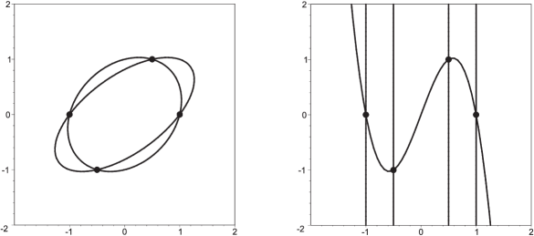
Figure A.4: Buchberger’s algorithm for the intersection of two ellipses.

Definition A.25

Let $S$ be a commutative ring with $1$ and $I\subset S$ an ideal. The set $S/I=\{\overline{f}=f+I\mid f\in S\}$ is a commutative ring with one with representative-wise addition $\overline{f}+\overline{g}:=\overline{f+g}$ and multiplication $\overline{f}\cdot\overline{g}:=\overline{f\cdot g}$.

Definition A.26

For our usual notation, and $I\subset R$ an ideal, the quotient ring $R/I$ is called the coordinate ring of $V(I)$.

In particular, if, as in Example A.24, the vanishing locus of a given ideal $I$ is finite, the coordinate ring $R/I$ allows us to directly analyize $V(I)$. The coordinate ring becomes computationally accessible via Gröbner bases.

Lemma A.27

If $I\subset R$ is an ideal and $\operatorname*{NF}(-,I)$ a reduced normal form, then

$$\phi:R/I\longrightarrow V=_{K}\left\langle x^{\alpha}\mid x^{\alpha}\notin L(I)\right\rangle\text{, \quad}\overline{f}\longmapsto\operatorname*{NF}(f,I)$$

is an isomorphism of $K$-vector spaces. With the multiplication on $V$ induced by applying $\operatorname*{NF}(-,I)$ after the respective operation in $R$, it becomes an isomorphism of $K$-algebras.

Theorem A.28

Let $K=\overline{K}$, $I\subset R$. Then the following are equivalent:

1. $\left|V\left(I\right)\right|<\infty$

2. If $G$ is a Gröbner basis of $I$, then for every $i$ there is a $g\in G$ with $L(g)=x_{i}^{\alpha_{i}}$ and $\alpha_{i}\geq 0$.

3. $\dim_{K}(R/I)<\infty$.

Theorem A.29

In the setting of the previous theorem,

$$\left|V\left(I\right)\right|\leq\dim_{K}\left(R/I\right)$$

and equality holds if $I$ is a radical ideal.

Definition A.30

With respect to the basis $\mathcal{B}=\left\{x^{\alpha}\mid x^{\alpha}\notin L(I)\right\}=:\{m_{1},\ldots,m_{r}\}$ of $V$, multiplication $\overline{f}\cdot$ by $\overline{f}$ in $R/I$ is given by matrix multiplication with the representing matrix

$$M_{f}:=M_{\mathcal{B}}^{\mathcal{B}}(\overline{f}\cdot)=(a_{ij})_{i,j=1,\ldots,r}$$

defined by

$$\overline{f}\cdot\bar{m}_{j}=\sum_{i=1}^{r}a_{ij}\bar{m}_{i}$$ (A.1)

The matrix $M_{f}$ is called the companion matrix of $f$.

Remark A.31

Passing from $\overline{f}\cdot$ to $M_{f}$ is a well-defined isomorphism of $K$-algebras from $R/I$ to a subalgebra of $\operatorname*{Mat}_{n\times n}(K)$: We have $M_{f}=M_{g}$ if an only if $\overline{f}=\overline{g}$, and $M_{f+g}=M_{f}+M_{g}$ and $M_{f\cdot g}=M_{f}\cdot M_{g}=M_{g}\cdot M_{f}$.

Definition A.32

If $M_{g}$ is invertible, then the companion matrix of the rational function $f/g$ $\in\operatorname{quot}(R)$ is $M_{f/g}=M_{f}\cdot M_{g}^{-1}$.

Remark A.33

Assume that $K=\overline{K}$ and $I$ is radical, and write $V(I)=\left\{p_{1},\ldots,p_{r}\right\}$. Then the sum of the values of $f\in R$ over the $p_{i}$ can be computed as the trace

$$\sum_{i=1}^{r}f(p_{i})=\operatorname{Tr}M_{f}\text{.}$$ (A.2)

A.2 Implementation notes

From the general introduction above, we see that if a physical quantity is expressed as a rational function summed over all Bethe roots, it can be calculated as the trace of the companion matrix (A.2). In practice, the efficient implementation of this method is a non-trivial task, especially for our case with two parameters (anisotropy parameter $q$ and the twist $\rho^{2}$). This is mainly due to two reasons. To start with, the ZRC from the rational $Q$-system, which are obtained by taking polynomial remainders, involve complicated coefficients which are rational functions of $q$ and $\rho$. Second, the algebro-geometric computation makes such complications proliferate and lead to bulky expressions in the intermediate steps. On the other hand, we know the final results that we are after have some simple structures, e.g. they are a polynomial in $\mathfrak{m}$ with integer coefficients. Therefore our strategy is to perform the computation for different sets of fixed numbers $(q,\rho)$ and then use proper interpolation formulae to find the final result.

In more details, when computing the Gröbner basis, we consider $\mathbb{Q}$-valued $\mathfrak{m}$ and a constant $\rho$, and perform the Gröbner-basis computation. Here $\mathfrak{m}=-q-q^{-1}$ in the usual parametrization. Note that the choice of $\mathfrak{m}$ should avoid the singular values of $q$. The Gröbner-basis computation with differnt $\mathbb{Q}$-valued $\mathfrak{m}$ and a constant $\rho$ can be parallelized on different cores or computer nodes. We observe that the computation time for different values is roughly the same, so the parallelization is very efficient. The Gröbner-basis computation is powered by the computer algebra system Singular [24].

Secondly, for each value of $\mathfrak{m}$ and $\rho$, once the Gröbner basis is obtained, we use (A.1) to get the companion matrix. Then the formula (A.2) is used to compute the corresponding value of the partition function. In this step, the linear-algebra related computations were done using Singular. Here we emphasize one subtlety in this step: the companion matrix of a polynomial’s power, $M_{f^{n}}$, is needed for our computation. In practice, $f^{n}$ may be a huge polynomial with a high degree and to handle such an object requires a lot of RAM. One might seek the help from the property of a companion matrix,

$$M_{f^{n}}=(M_{f})^{n},$$ (A.3)

and carry out the power computation on matrices instead of on polynomials. However, in practice, we find that $M_{f}$ may be a dense matrix and such a matrix-power computation is not particularly efficient. Therefore, we consider the remainder $\bar{f}$ of $f$ divided by the Gröbner basis and the following relation,

$$M_{f^{n}}=M_{\bar{f}^{n}}\,.$$ (A.4)

For the computation of $\bar{f}$’s power, after each multiplication, we divide the intermediate result towards the Gröbner basis and take the remainder. In the way, the power computation is both efficient and RAM economical.

Finally, from the previous two steps, we get the partition function’s values for a list of $\mathbb{Q}$-values of $\mathfrak{m}$ and the constant $\rho$. Note that the partion function is not a polynomial in $q$ but a polynomial in $\mathfrak{m}$. Then we do a standard Newton-polynomial interpolation in $\mathfrak{m}$ to get the fully analytic partition function. This step is also powered by Singular.

We observe that these computations over finite fields are much faster than over rational numbers. The results over finite fields can be further lifted to rational numbers. Although in this paper, our computation is done with rational numbers, the finite-field method is promising for future computations.

Appendix B Partition function results

In the appendix, we give some results for the partition functions on $L\times L$ tori.

B.1 Loop model

$$Z(2,2) = 8\mathfrak{m}+8\mathfrak{m}^{2}\,,$$ (B.1a)

$$Z(4,4) = 8192\mathfrak{m}+21480\mathfrak{m}^{2}+21632\mathfrak{m}^{3}+10870\mathfrak{m}^{4}+2912\mathfrak{m}^{5}+416\mathfrak{m}^{6}+32\mathfrak{m}^{7}+2\mathfrak{m}^{8}\,,$$ (B.1b)

$$Z(6,6) = 933120000\mathfrak{m}+4805838000\mathfrak{m}^{2}+11273241408\mathfrak{m}^{3}+16045483644\mathfrak{m}^{4}+15559888944\mathfrak{m}^{5}+10937711238\mathfrak{m}^{6}+$$ (B.1c)

$$5789102208\mathfrak{m}^{7}+2366852316\mathfrak{m}^{8}+761946512\mathfrak{m}^{9}+196445178\mathfrak{m}^{10}+41330040\mathfrak{m}^{11}+7264344\mathfrak{m}^{12}+$$

$$1093680\mathfrak{m}^{13}+142350\mathfrak{m}^{14}+15504\mathfrak{m}^{15}+1296\mathfrak{m}^{16}+72\mathfrak{m}^{17}+2\mathfrak{m}^{18}\,,$$

$$Z(8,8) = 11399736556781568\mathfrak{m}+98753367284702880\mathfrak{m}^{2}+408215404199487488\mathfrak{m}^{3}+1073458486777028536\mathfrak{m}^{4}+$$ (B.1d)

$$2019645508709576192\mathfrak{m}^{5}+2898901544581297904\mathfrak{m}^{6}+3305315996372032512\mathfrak{m}^{7}+3077975536301413966\mathfrak{m}^{8}+$$

$$2388746188868407168\mathfrak{m}^{9}+1568981821963717920\mathfrak{m}^{10}+882883392305392000\mathfrak{m}^{11}+429902632210623280\mathfrak{m}^{12}+$$

$$182694107341546624\mathfrak{m}^{13}+68277701699851360\mathfrak{m}^{14}+22602553762014464\mathfrak{m}^{15}+6675367972759608\mathfrak{m}^{16}+$$

$$1772015524475520\mathfrak{m}^{17}+426101046596224\mathfrak{m}^{18}+93529351075584\mathfrak{m}^{19}+18862409602432\mathfrak{m}^{20}+$$

$$3507873891968\mathfrak{m}^{21}+601033262944\mathfrak{m}^{22}+94278773888\mathfrak{m}^{23}+13385143248\mathfrak{m}^{24}+1693508480\mathfrak{m}^{25}+$$

$$187378704\mathfrak{m}^{26}+17724928\mathfrak{m}^{27}+1392704\mathfrak{m}^{28}+87296\mathfrak{m}^{29}+4096\mathfrak{m}^{30}+128\mathfrak{m}^{31}+2\mathfrak{m}^{32}\,,$$

B.2 Potts model

$$Z(2,2) = 4\mathfrak{m}^{3}+7\mathfrak{m}^{4}+4\mathfrak{m}^{5}+\mathfrak{m}^{6}\,,$$ (B.2a)

$$Z(4,4) = 4096\mathfrak{m}^{9}+14056\mathfrak{m}^{10}+20064\mathfrak{m}^{11}+15866\mathfrak{m}^{12}+7904\mathfrak{m}^{13}+2716\mathfrak{m}^{14}+688\mathfrak{m}^{15}+129\mathfrak{m}^{16}+16\mathfrak{m}^{17}+\mathfrak{m}^{18}\,,$$ (B.2b)

$$Z(6,6) = 466560000\mathfrak{m}^{19}+2787706800\mathfrak{m}^{20}+7672413504\mathfrak{m}^{21}+2973997052\mathfrak{m}^{22}+15177608016\mathfrak{m}^{23}+13124121918\mathfrak{m}^{24}+$$ (B.2c)

$$8762270208\mathfrak{m}^{25}+4665716646\mathfrak{m}^{26}+2034402892\mathfrak{m}^{27}+742926501\mathfrak{m}^{28}+231451420\mathfrak{m}^{29}+62280555\mathfrak{m}^{30}+$$

$$14527800\mathfrak{m}^{31}+2918460\mathfrak{m}^{32}+496704\mathfrak{m}^{33}+69786\mathfrak{m}^{34}+7788\mathfrak{m}^{35}+649\mathfrak{m}^{36}+36\mathfrak{m}^{37}+\mathfrak{m}^{38}\,,$$

$$Z(8,8) = 5699868278390784\mathfrak{m}^{33}+54114294708625056\mathfrak{m}^{34}+245768814667966464\mathfrak{m}^{35}+712035958563348408\mathfrak{m}^{36}+$$

$$1480662138337422848\mathfrak{m}^{37}+2357818409374775024\mathfrak{m}^{38}+2995910569524062208\mathfrak{m}^{39}+3125648118282379662\mathfrak{m}^{40}+$$

$$2735085239079547520\mathfrak{m}^{41}+2040940779811857696\mathfrak{m}^{42}+1316441555189606912\mathfrak{m}^{43}+742458511348946736\mathfrak{m}^{44}+$$

$$369838333858415104\mathfrak{m}^{45}+164188589066409952\mathfrak{m}^{46}+65497210088055296\mathfrak{m}^{47}+23650757646619036\mathfrak{m}^{48}+$$

$$7779745847048704\mathfrak{m}^{49}+2343002229704412\mathfrak{m}^{50}+648253398180864\mathfrak{m}^{51}+165020839221248\mathfrak{m}^{52}+$$

$$38632494033536\mathfrak{m}^{53}+8297778619424\mathfrak{m}^{54}+1628522160640\mathfrak{m}^{55}+290394241736\mathfrak{m}^{56}+46707916288\mathfrak{m}^{57}+$$

$$6714987800\mathfrak{m}^{58}+853018752\mathfrak{m}^{59}+94339168\mathfrak{m}^{60}+8906112\mathfrak{m}^{61}+698400\mathfrak{m}^{62}+43712\mathfrak{m}^{63}+2049\mathfrak{m}^{64}+64\mathfrak{m}^{65}+\mathfrak{m}^{66}\,.$$

References

- [1] Y. Jiang and Y. Zhang, “Algebraic geometry and Bethe ansatz. Part I. The quotient ring for BAE,” JHEP 03 (2018) 087, arXiv:1710.04693 [hep-th].
- [2] R. P. Langlands and Y. Saint-Aubin, “Algebro-geometric aspects of the Bethe equations,” in Strings and Symmetries, pp. 40–53. Springer, 1995.
- [3] R. P. Langlands and Y. Saint-Aubin, “Aspects combinatoires des équations de Bethe”, Advances in mathematical sciences 25 (1997) 231-302
- [4] J. L. Jacobsen, Y. Jiang, and Y. Zhang, “Torus partition function of the six-vertex model from algebraic geometry,” JHEP 03 (2019) 152, arXiv:1812.00447 [hep-th].
- [5] Z. Bajnok, J. L. Jacobsen, Y. Jiang, R. I. Nepomechie, and Y. Zhang, “Cylinder partition function of the 6-vertex model from algebraic geometry,” JHEP 06 (2020) 169, arXiv:2002.09019 [hep-th].
- [6] Y. Jiang, R. Wen, and Y. Zhang, “Exact quench dynamics from algebraic geometry,” arXiv:2109.10568 [hep-th].
- [7] J. J. Graham and G. I. Lehrer, “The representation theory of affine Temperley-Lieb algebras,” L’Ens. Math. 44 (1998) 173–218.
- [8] P. Martin and H. Saleur, “The blob algebra and the periodic Temperley-Lieb algebra,” Lett. Math. Phys. 30 no. 3, (1994) 189–206.
- [9] P. Martin and H. Saleur, “On an algebraic approach to higher dimensional statistical mechanics,” Comm. Math. Phys. 158 no. 1, (1993) 155–190.
- [10] H. N. Temperley and E. H. Lieb, “Relations between the ‘percolation’ and ‘colouring’ problem and other graph-theoretical problems associated with regular planar lattices: some exact results for the ‘percolation’ problem,” Proc. Roy. Soc. Lon. A 322 no. 1549, (1971) 251–280.
- [11] R. Baxter, S. Kelland, and F. Wu, “Equivalence of the Potts model or Whitney polynomial with an ice-type model,” J. Phys. A: Math. Gen. 9 (1976) 397.
- [12] C. Fortuin and P. Kasteleyn, “On the random-cluster model: I. Introduction and relation to other models,” Physica 57 (1972) 536–564.
- [13] V. F. Jones, “A quotient of the affine Hecke algebra in the Brauer algebra,” L’Ens. Math. 40 (1994) 313–313.
- [14] N. Read and H. Saleur, “Enlarged symmetry algebras of spin chains, loop models, and S-matrices,” Nucl. Phys. B 777 (2007) 263–315, arXiv:cond-mat/0701259.
- [15] V. F. R. Jones, “Index for subfactors,” Invent. Math. 72 (1983) 1–25.
- [16] L. Grans-Samuelsson, L. Liu, Y. He, J. L. Jacobsen, and H. Saleur, “The action of the Virasoro algebra in the two-dimensional Potts and loop models at generic ,” JHEP 10 (2020) 109, arXiv:2007.11539 [hep-th].
- [17] J. L. Jacobsen and H. Saleur, “Bootstrap approach to geometrical four-point functions in the two-dimensional critical -state Potts model: A study of the -channel spectra,” JHEP 01 (2019) 084, arXiv:1809.02191 [math-ph].
- [18] A. M. Gainutdinov, J. L. Jacobsen, and H. Saleur, “A fusion for the periodic Temperley-Lieb algebra and its continuum limit,” JHEP 11 (2018) 117, arXiv:1712.07076 [hep-th].
- [19] W. M. Koo and H. Saleur, “Representations of the Virasoro algebra from lattice models,” Nucl. Phys. B 426 (1994) 459–504, arXiv:hep-th/9312156.
- [20] G. H. Hardy, E. M. Wright, et al., An introduction to the theory of numbers. Oxford University Press, 1979.
- [21] P. Di Francesco, H. Saleur, and J.-B. Zuber, “Relations between the Coulomb gas picture and conformal invariance of two-dimensional critical models,” J. Stat. Phys. 49 no. 1, (1987) 57–79.
- [22] N. Read and H. Saleur, “Exact spectra of conformal supersymmetric nonlinear sigma models in two dimensions,” Nucl. Phys. B 613 (2001) 409, arXiv:hep-th/0106124.
- [23] J.-F. Richard and J. L. Jacobsen, “Eigenvalue amplitudes of the Potts model on a torus,” Nucl. Phys. B 769 (2007) 256–274, arXiv:math-ph/0608055.
- [24] W. Decker, G.-M. Greuel, G. Pfister, and H. Schönemann, “Singular 4-1-3 — A computer algebra system for polynomial computations.” http://www.singular.uni-kl.de, 2020.
- [25] G. Kirchhoff, “Ueber die Auflösung der Gleichungen, auf welche man bei der Untersuchung der linearen Vertheilung galvanischer Ströme geführt wird,” Ann. Phys. Chem. 72 (1847) 497–508.
- [26] S. Caracciolo, J. L. Jacobsen, H. Saleur, A. D. Sokal, and A. Sportiello, “Fermionic field theory for trees and forests,” Phys. Rev. Lett. 93 (2004) 080601, arXiv:0403271 [cond-mat].
- [27] R. B. Potts, “Some generalized order-disorder transformations,” Math. Proc. Cambridge Phil. Soc. 48 (1952) 106–109.
- [28] R. J. Baxter, “Potts model at the critical temperature,” J. Phys. C: Solid State Phys. 6 (1973) L445.
- [29] J. L. Jacobsen, “High-precision percolation thresholds and Potts-model critical manifolds from graph polynomials,” J. Phys. A: Math. Theor. 47 (2014) 135001, arXiv:1401.7847.
- [30] C. Marboe and D. Volin, “Fast analytic solver of rational Bethe equations,” J. Phys. A 50 no. 20, (2017) 204002, arXiv:1608.06504 [math-ph].
- [31] E. Granet and J. L. Jacobsen, “On zero-remainder conditions in the Bethe ansatz,” arXiv:1910.07797 [hep-th].
- [32] Z. Bajnok, E. Granet, J. L. Jacobsen, and R. I. Nepomechie, “On generalized -systems,” arXiv:1910.07805 [hep-th].
- [33] V. Kazakov, S. Leurent, and D. Volin, “T-system on T-hook: Grassmannian Solution and Twisted Quantum Spectral Curve,” JHEP 12 (2016) 044, arXiv:1510.02100 [hep-th].
- [34] J. Beraha, S. an Kahane and N. J. Weiss, “Limits of zeroes of recursively defined polynomials,” Proc. Nat. Acad. Sci. 72 (1975) 4209.
- [35] J. L. Jacobsen, “Conformal field theory applied to loop models,” in Polygons, polyominoes and polycubes, pp. 347–424. Springer, 2009.
- [36] J. L. Jacobsen, S. Ribault, and H. Saleur, “Phase diagram of the Potts model in the complex plane,” in preparation (2022) .
- [37] A. Lafay, A. M. Gainutdinov, and J. L. Jacobsen, “ web models and spin interfaces,” J. Stat. Mech.: Theor. Exp. (2021) 053104, arXiv:2101.00282 [cond-mat].
- [38] A. Lafay, A. M. Gainutdinov, and J. L. Jacobsen, “ web models: Locality, phase diagram and geometrical defects,” Nucl. Phys. B in press (2021) , arXiv:2107.10106 [cond-mat].
- [39] V. Pasquier and H. Saleur, “Common structures between finite systems and conformal field theories through quantum groups,” Nucl. Phys. B 330 (1990) 523–556.
- [40] D. Ridout and Y. Saint-Aubin, “Standard modules, induction and the structure of the Temperley-Lieb algebra,” Adv. Theor. Math. Phys. 18 (2014) 957–1041.
- [41] J. Dubail, J. L. Jacobsen, and H. Saleur, “Conformal field theory at central charge : a measure of the indecomposability (b) parameters,” Nucl. Phys. B 834 (2010) 399–422, arXiv:1001.1151 [math-ph].
- [42] R. Vasseur, J. L. Jacobsen, and H. Saleur, “Indecomposability parameters in chiral logarithmic conformal field theory,” Nucl. Phys. B 851 (2011) 314–345, arXiv:1103.3134 [math-ph].
- [43] A. Gainutdinov, J. L. Jacobsen, N. Read, H. Saleur, and R. Vasseur, “Logarithmic conformal field theory: a lattice approach,” J. Phys. A: Math. Theor. (2013) 494012, arXiv:1303.2082 [hep-th].
- [44] R. J. Baxter, “Completeness of the Bethe ansatz for the six and eight-vertex models,” J. Stat. Phys. 108 no. 1, (2002) 1–48.
- [45] N. A. Nekrasov and S. L. Shatashvili, “Supersymmetric vacua and Bethe ansatz,” Nucl. Phys. B Proc. Suppl. 192-193 (2009) 91–112, arXiv:0901.4744 [hep-th].
- [46] N. A. Nekrasov and S. L. Shatashvili, “Quantization of integrable systems and four dimensional gauge theories,” in 16th International Congress on Mathematical Physics, pp. 265–289. 8, 2009. arXiv:0908.4052 [hep-th].
- [47] N. A. Nekrasov and S. L. Shatashvili, “Bethe/Gauge correspondence on curved spaces,” JHEP 01 (2015) 100, arXiv:1405.6046 [hep-th].
- [48] C. Closset and H. Kim, “Comments on twisted indices in 3d supersymmetric gauge theories,” JHEP 08 (2016) 059, arXiv:1605.06531 [hep-th].
- [49] G. Greuel and G. Pfister, A singular introduction to commutative algebra. Springer, 2002. https://books.google.de/books?id=2fkHjk9stskC.
- [50] J. Böhm, “Computer algebra.” https://www.mathematik.uni-kl.de/~boehm/lehre/20_CA/ca.pdf, 2020.
- [51] J.-C. Faugère, “A new efficient algorithm for computing Gröbner bases (F4),” Journal of Pure and Applied Algebra 139 no. 1, (1999) 61–88. https://www.sciencedirect.com/science/article/pii/S0022404999000055.