Neural Tangent Kernel Analysis of Deep Narrow Neural Networks

Abstract

The tremendous recent progress in analyzing the training dynamics of overparameterized neural networks has primarily focused on wide networks and therefore does not sufficiently address the role of depth in deep learning. In this work, we present the first trainability guarantee of infinitely deep but narrow neural networks. We study the infinite-depth limit of a multilayer perceptron (MLP) with a specific initialization and establish a trainability guarantee using the NTK theory. We then extend the analysis to an infinitely deep convolutional neural network (CNN) and perform brief experiments.

1 Introduction

Despite the remarkable experimental advancements of deep learning in many domains, a theoretical understanding behind this success remains elusive. Recently, significant progress has been made by analyzing limits of infinitely large neural networks to obtain provable guarantees. The neural tangent kernel (NTK) and the mean-field (MF) theory are the most prominent results.

However, these prior analyses primarily focus on the infinite width limit and therefore do not sufficiently address the role of depth in deep learning. After all, substantial experimental evidence indicates that depth is indeed an essential component to the success of modern deep neural networks. Analyses directly addressing the limit of infinite depth may lead to an understanding of the role of depth.

In this work, we present the first trainability guarantee of infinitely deep but narrow neural networks. We study the infinite-depth limit of a multilayer perceptron (MLP) with a very specific initialization and establish a trainability guarantee using the NTK theory. The MLP uses ReLU activation functions and has width on the order of input dimension + output dimension. Furthermore, we extend the analysis to an infinitely deep convolutional neural network (CNN) and perform brief experiments.

1.1 Prior works

The classical universal approximation theorem establishes that wide 2-layer neural networks can approximate any continuous function (Cybenko, 1989; Funahashi, 1989). Extensions and generalizations (Hornik, 1991; Leshno et al., 1993; Jones, 1992; Barron, 1993; Pinkus, 1999) and random feature learning (Rahimi & Recht, 2007, 2008a, 2008b), a constructive version of the universal approximation theorem, use large width in their analyses. As overparameterization got recognized as a key component in understanding the performance of deep learning (Zhang et al., 2017), analyses of large neural networks started to appear in the literature (Soltanolkotabi et al., 2019; Allen-Zhu et al., 2019; Du et al., 2019a, b; Zou et al., 2020; Li & Liang, 2018), and their infinite-width limits such as neural network as Gaussian process (NNGP) (Neal, 1994, 1996; Williams, 1997; Lee et al., 2018; Matthews et al., 2018; Novak et al., 2019), neural tangent kernel (NTK) (Jacot et al., 2018), and mean-field (MF) (Mei et al., 2018; Chizat & Bach, 2018; Rotskoff & Vanden-Eijnden, 2018; Rotskoff et al., 2019; Sirignano & Spiliopoulos, 2020a, b; Nguyen & Pham, 2021; Pham & Nguyen, 2021) were formulated. NNGP characterizes the neural network at initialization, while NTK and MF analyses provide guarantees of trainability with SGD. This line of research naturally raises the question of whether very deep neural networks also enjoy similar properties as wide neural networks, especially given the importance of depth in modern deep learning.

The analogous line of research for very deep neural networks has a shorter history. Universality of deep narrow neural networks (Lu et al., 2017; Hanin & Sellke, 2017; Lin & Jegelka, 2018; Hanin, 2019; Kidger & Lyons, 2020; Park et al., 2021; Tabuada & Gharesifard, 2021), lower bounds on the minimum width necessary for universality (Lu et al., 2017; Hanin & Sellke, 2017; Johnson, 2019; Park et al., 2021), and quantitative analyses showing the benefit of depth over width in approximating certain functions (Telgarsky, 2016) are all very recent developments. On the other hand, the neural ODE (Chen et al., 2018) is a continuous-depth model that can be considered an infinite-depth limit of a neural network with residual connections. Also stochastic extensions of neural ODE, viewing infinitely deep ResNets as diffusion processes, have been considered in (Peluchetti & Favaro, 2020, 2021). However, these continuous-depth limits do not come with any trainability or generalization guarantees. In the infinite width and depth limit, a quantitative universal approximation result has been established (Lu et al., 2021) and a trainability guarantee was obtained in setups combining the MF limit with the continuous-depth limit inspired by the neural ODE (Lu et al., 2020; Ding et al., 2021, 2022).

Efforts to understand the trainability of deep non-wide neural networks have been made. Arora et al. (2019a); Shamir (2019) establishes trainability guarantees for linear deep networks (no activation functions). Pennington et al. (2017) studied the so-called dynamic isometry property, Hanin (2018) studied the exploding and vanishing gradient problem for ReLU MLPs, and Huang et al. (2020) studied the NTK of deep MLPs and ResNets at initialization, but these results are limited to the state of the neural network at initialization and therefore do not directly establish guarantees on the training dynamics. To the best of our knowledge, no prior work has yet established a trainability guarantee on (non-linear) deep narrow neural networks.

Many extensions and variations of the NTK have been studied: NTK analysis with convolutional layers (Arora et al., 2019b; Yang, 2019), further refined analyses and experiments (Lee et al., 2019), NTK analysis with regularizers and noisy gradients (Chen et al., 2020), finite-width NTK analysis (Hanin & Nica, 2020), quantitative universality result of the NTK (Ji et al., 2020), generalization properties of overparameterized neural networks (Bietti & Mairal, 2019; Woodworth et al., 2020), unified analysis of NTK and MF (Geiger et al., 2020), notion of lazy training generalizing linearization effect of the NTK regime (Chizat et al., 2019), closed-form evaluations of NTK kernel values (Cho & Saul, 2009; Arora et al., 2019b), analyses of distribution shift and meta learning in the infinite-width regime (Adlam et al., 2021; Nguyen et al., 2021), library implementations of infinitely wide neural networks as kernel methods with NTK (Novak et al., 2020), empirical evaluation of finite vs. infinite neural networks (Lee et al., 2020), and constructing better-performing kernels with improved extrapolation of the standard initialization (Sohl-Dickstein et al., 2020). Such results have mostly focused on the analysis and application of wide, rather than deep, neural networks.

1.2 Contribution

In this work, we analyze the training dynamics of a deep narrow MLP and CNN without residual connections and establish trainability guarantees. To the best of our knowledge, this is the first trainability guarantee of deep narrow neural networks, with or without residual connections; prior trainability guarantees consider the infinite width or the infinite depth and width limits. Essential to our analysis is the particular choice of initialization, as very deep networks with the usual initialization schemes are known to not be trainable (He & Sun, 2015, Section 4.4), (Srivastava et al., 2015, Section 3.1), (Huang et al., 2020, Section 4.1). By considering the limit in which only the depth is infinite, we demonstrate that infinite depth is sufficient to obtain a neural network with trainability guarantees.

The key technical challenge of our work arises from bounding the variation of the scaled NTK in the infinite-depth limit via a delicate Lyapunov analysis. Our infinite-depth analysis requires that we control an infinite composition of layers and an infinite product of matrices, which is significantly more technical than the prior infinite-width analyses that can more directly apply the central limit theorem and law of large numbers.

The MLP we analyze is narrow in the sense that it is within a factor of 2 of the width lower bound for universal approximation (Park et al., 2021). In particular, the width does not depend on the number of data points.

2 Preliminaries and notation

In this section, we review the necessary background and set up the notation. We largely follow the notions of Jacot et al. (2018), although our notation has some minor differences.

Given a function $f_{\theta}(x)\in\mathbb{R}^{n}$ with $\theta\in\mathbb{R}^{p}$ and $x\in\mathbb{R}^{d}_{+}$, write $\partial_{\theta}f_{\theta}(x)\in\mathbb{R}^{n\times p}$ to denote the Jacobian matrix with respect to $\theta$. If $f_{\theta}(x)\in\mathbb{R}$ is scalar-valued, write $\nabla_{\theta}f_{\theta}(x)\in\mathbb{R}^{p\times 1}$ for the gradient. The gradient and Jacobian matrices are, by convention, transposes of each other, i.e., $\nabla_{\theta}f_{\theta}(x)=(\partial_{\theta}f_{\theta}(x))^{\intercal}$. Write $\|\cdot\|$ to denote the standard Euclidean norm for vectors and the standard operator norm for matrices. Write $\left\langle\cdot,\cdot\right\rangle$ for the vector and Frobenius inner products. Write $\mathbb{R}^{d}_{+}\subset\mathbb{R}^{d}$ for the strict positive orthant, i.e., $\mathbb{R}^{d}_{+}$ is the set of vectors with element-wise positive entries. Write $\stackrel{{\scriptstyle p}}{{\rightarrow}}$ to denote convergence in probability. Write $g\sim\mathcal{GP}(\mu,\Sigma)$ to denote that $g$ is a Gaussian process with mean $\mu(x)$ and covariance kernel $\Sigma(x,x^{\prime})$ (Rasmussen, 2004; Rasmussen & Williams, 2005).

Let $p^{in}$ be the empirical distribution on a training dataset $x_{1},x_{2},\dots,x_{N}\in\mathbb{R}^{d_{in}}_{+}$, which we assume are element-wise positive. Let ${\cal F}=\{f\colon\mathbb{R}^{d_{in}}_{+}\rightarrow\mathbb{R}^{d_{out}}\}$ be the function space with a seminorm $\left\|{\cdot}\right\|_{p^{in}}$ induced by the bilinear map

$$\langle f,g\rangle_{p^{in}} =\mathbb{E}_{x\sim p^{in}}[f(x)^{\intercal}g(x)].$$

If $W$ is a matrix-valued function, write

$$\left\|{W}\right\|_{p^{in}}^{2}=\mathbb{E}_{x\sim p^{in}}\|W(x)\|^{2},$$

where $\|\cdot\|$ here is the operator norm.

Kernel gradient flow.

Let $\mathcal{L}\colon{\cal F}\rightarrow\mathbb{R}$ be a functional loss. We primarily consider $\mathcal{L}(f)=\frac{1}{2}\left\|{f-f^{\star}}\right\|_{p^{in}}^{2}$ with a given target function $f^{\star}$. We train a neural network $f_{\theta}$ by solving

$$\begin{array}[]{ll}\underset{\theta}{\mbox{minimize}}&\mathcal{L}(f_{\theta}).\end{array}$$

Let ${\cal F}^{*}$ denote the dual of ${\cal F}$ with respect to $p^{in}$. So ${\cal F}^{*}$ consists of linear maps $\langle\delta,\cdot\rangle_{p^{in}}$ for some $\delta\in{\cal F}$. Let $\partial_{f}\mathcal{L}|_{f_{0}}$ denote the functional derivative of the loss at $f_{0}$. Since $\partial_{f}\mathcal{L}|_{f_{0}}\in{\cal F}^{*}$, there exists a corresponding dual element $\delta|_{f_{0}}\in{\cal F}$, where $\partial_{f}\mathcal{L}|_{f_{0}}=\langle\delta|_{f_{0}},\cdot\rangle_{p^{in}}$. To clarify, $\delta|_{f_{0}}(x)$ is defined to be a length $d_{out}$ column vector.

A multi-dimensional kernel $K\colon\mathbb{R}^{d_{\mathrm{in}}}_{+}\times\mathbb{R}^{d_{\mathrm{in}}}_{+}\to\mathbb{R}^{d_{\mathrm{out}}\times d_{\mathrm{out}}}$ is a function such that $K(x,x^{\prime})=K(x^{\prime},x)^{\intercal}$ for all $x,x^{\prime}\in\mathbb{R}^{d_{\mathrm{in}}}_{+}$. A multi-dimensional kernel is positive semidefinite if

$$\mathbb{E}_{x,x^{\prime}\sim p^{in}}\left[f(x)^{\intercal}K(x,x^{\prime})f(x^{\prime})\right]\geq 0$$

for all $f\in{\cal F}$ and (strictly) positive definite if the inequality holds strictly when $\left\|{f}\right\|_{p^{in}}\neq 0$. To clarify, $\mathbb{E}_{x,x^{\prime}\sim p^{in}}$ denotes the expectation with respect to $x$ and $x^{\prime}$ sampled independently from $p^{in}$. The kernel gradient of $\mathcal{L}$ at $f_{0}$ with respect to the kernel $K$ is defined as

$$\nabla_{K}\mathcal{L}|_{f_{0}}(x)=\mathbb{E}_{x^{\prime}\sim p^{in}}\left[{K(x,x^{\prime})\delta|_{f_{0}}(x^{\prime})}\right]$$

for all $x\in\mathbb{R}_{+}^{d_{\mathrm{in}}}$. We say a time-dependent function $f_{t}$ follows the kernel gradient flow with respect to $K$ if

$$\partial_{t}f_{t}(x)=-\nabla_{K}\mathcal{L}|_{f_{t}}(x)$$

for all $t>0$ and $x\in\mathbb{R}^{d_{\mathrm{in}}}_{+}$. During the kernel gradient flow, the loss $\mathcal{L}(f_{t})$ evolves as

$$\partial_{t}\mathcal{L}|_{f_{t}}= -\mathbb{E}_{x,x^{\prime}\sim p^{in}}\left[\delta|_{f_{t}}(x)^{\intercal}K(x,x^{\prime})\delta|_{f_{t}}(x^{\prime})\right].$$

If $K$ is positive definite and if certain regularity conditions hold, then kernel gradient flow converges a critical point and it converges to a global minimum if $\mathcal{L}$ is convex and bounded from below.

Neural tangent kernel.

Given a neural network $f_{\theta(t)}$, Jacot et al. (2018) defines the neural tangent kernel (NTK) at time $t$ as

$$\Theta_{t}(x,x^{\prime})=\partial_{\theta}f_{\theta(t)}(x)\left({\partial_{\theta}f_{\theta(t)}(x^{\prime})}\right)^{\intercal},$$

which, by definition, is a positive semidefinite kernel. Jacot et al. (2018) pointed out that a neural network trained with gradient flow, which we define and discuss in Section 3.2, can be viewed as kernel gradient flow with respect to $\Theta_{t}$, i.e.,

$$\partial_{t}f_{\theta(t)}(x)=-\nabla_{\Theta_{t}}\mathcal{L}|_{f_{t}}(x).$$

However, even though $\Theta_{t}$ is always positive semidefinite, the time-dependence of $\Theta_{t}$ makes the training dynamics non-convex and prevents one from establishing trainability guarantees in general. The contribution of Jacot et al. (2018) is showing that $\Theta_{t}\stackrel{{\scriptstyle p}}{{\rightarrow}}\Theta$ in an appropriate infinite-width limit, where $\Theta$ is a fixed limit that does not depend on time. Then, since $\Theta$ is fixed, kernel gradient flow generically converges provided that the loss $\mathcal{L}$ is convex.

3 NTK analysis of infinitely deep MLP

Consider an $L$-layer multilayer perceptron (MLP) $f^{L}_{\theta}\colon\mathbb{R}^{d_{\mathrm{in}}}_{+}\rightarrow\mathbb{R}^{d_{\mathrm{out}}}$ parameterized by $\theta$, where the input $x\in\mathbb{R}^{d_{\mathrm{in}}}_{+}$ is a $d_{\mathrm{in}}$-dimensional vector with positive entries and the output is a $d_{\mathrm{out}}$-dimensional vector. The network consists of $L-1$ fully connected hidden layers with uniform width $d_{\mathrm{in}}+d_{\mathrm{out}}+1$, each followed by the ReLU activation function. The final output layer has width $d_{\mathrm{out}}$ and is not followed by an activation function.

Let us set up specific notation. Define the pre-activation values as

$$f^{1}_{\theta^{(1)}}(x) =W^{1}x+b^{1}$$

$$f^{l}_{\theta^{(l)}}(x) =W^{l}\sigma(f^{l-1}_{\theta^{(l-1)}}(x))+b^{l},\qquad 2\leq l\leq L.$$

We use ReLU for the activation $\sigma$. The weight matrices have dimension $W^{1}\in\mathbb{R}^{(d_{\mathrm{in}}+d_{\mathrm{out}}+1)\times{d_{\mathrm{in}}}}$, $W^{2},\dots,W^{L-1}\in\mathbb{R}^{(d_{\mathrm{in}}+d_{\mathrm{out}}+1)\times(d_{\mathrm{in}}+d_{\mathrm{out}}+1)}$, and $W^{L}\in\mathbb{R}^{d_{\mathrm{out}}\times(d_{\mathrm{in}}+d_{\mathrm{out}}+1)}$. The bias vectors have dimension $b^{1},\dots,b^{L-1}\in\mathbb{R}^{(d_{\mathrm{in}}+d_{\mathrm{out}}+1)\times 1}$ and $b^{L}\in\mathbb{R}^{d_{\mathrm{out}}\times 1}$. For $1\leq l\leq L$, write $\theta^{(l)}=\{W^{i},b^{i}:i\leq l\}$ to denote the collection of parameters up to $l$-th layer. Let $f^{L}_{\theta}=f^{L}_{\theta^{(L)}}$.

3.1 Initialization

Motivated by Kidger & Lyons (2020), initialize the weights of our $L$-layer MLP $f^{L}_{\theta}$ as follows:

$$W^{1} =\begin{bmatrix}C_{L}I_{d_{\mathrm{in}}}\\ u^{1}\\ 0_{d_{\mathrm{out}}\times d_{\mathrm{in}}}\end{bmatrix}$$

$$W^{l} =\begin{bmatrix}I_{d_{\mathrm{in}}}&0_{d_{\mathrm{in}}\times 1}&0_{d_{\mathrm{in}}\times d_{\mathrm{out}}}\\ u^{l}&0_{1\times 1}&0_{1\times d_{\mathrm{out}}}\\ 0_{d_{\mathrm{out}}\times d_{\mathrm{in}}}&0_{d_{\mathrm{out}}\times 1}&I_{d_{\mathrm{out}}}\end{bmatrix}$$

$$W^{L} =\begin{bmatrix}0_{d_{\mathrm{out}}\times d_{\mathrm{in}}}&0_{d_{\mathrm{out}}\times 1}&I_{d_{\mathrm{out}}}\end{bmatrix}$$

for $2\leq l\leq L-1$, where $u^{l}\in\mathbb{R}^{1\times d_{\mathrm{in}}}$ is randomly sampled $u^{l}_{i}\stackrel{{\scriptstyle iid}}{{\sim}}\mathcal{N}(0,\frac{1}{d_{\mathrm{in}}}\rho^{2})$ for $1\leq l\leq L-1$. Here, $I_{d}$ is the $d\times d$ identity matrix and $0_{m\times n}$ is the $m$ by $n$ matrix with all zero entries, $C_{L}>0$ is a scalar growing as a function of $L$ at a rate satisfying $L^{2}/C_{L}\rightarrow 0$, and $\rho>0$ is a fixed variance parameter. Initializes the biases as follows:

$$b^{1} =\begin{bmatrix}0_{d_{\mathrm{in}}\times 1}\\ v^{1}\\ C_{L}\mathbbm{1}_{d_{\mathrm{out}}}\end{bmatrix}$$

$$b^{l} =\begin{bmatrix}0_{d_{\mathrm{in}}\times 1}\\ v^{l}\\ 0_{d_{\mathrm{out}}\times 1}\end{bmatrix}$$

$$b^{L} =\begin{bmatrix}-C_{L}\mathbbm{1}_{d_{\mathrm{out}}}\end{bmatrix}$$

for $2\leq l\leq L-1$, where $v^{l}\in\mathbb{R}$ is randomly sampled $v^{l}\stackrel{{\scriptstyle iid}}{{\sim}}\mathcal{N}(0,C_{L}^{2}\beta^{2})$ for $1\leq l\leq L-1$. Here, $\beta>0$ is a fixed variance parameter. Note that $\mathbbm{1}_{k}\in\mathbb{R}^{{k\times 1}}$ is the vector whose entries are all $1$. Figure 1 illustrates this initialization scheme.

We clarify that while we use many specific non-random initializations, those parameters are not fixed throughout training. In other words, all parameters are trainable, just as one would expect from a standard MLP.

Kidger & Lyons (2020) used a similar construction to establish a universal approximation result for deep MLPs by showing that their deep MLP mimics a 2-layer wide MLP. However, their main concern is the existence of a weight configuration that approximates a given function, which does not guarantee that such a configuration can be found through training. On the other hand, we propose an explicit initialization and establish a trainability guarantee; our network outputs 0 at initialization and converges to the desired configuration through training.

Figure 1: Initialization of deep MLP with $d_{in}=3$ and $d_{out}=2$. Intermediate layers have width $d_{in}+1+d_{out}$. Line styles indicate types of weight initializations (solid:1, double:$C_{L}$, dash:Gaussian, none:0). Box styles indicate types of bias initializations (solid:0, dash:Gaussian, double:$C_{L}$, double-dash:$-C_{L}$).

3.2 Gradient flow and neural tangent kernel

We are now ready to describe the training of our neural network $f^{L}_{\theta}$ via gradient flow, a continuous-time model of gradient descent. Since our initialization scales the input by $C_{L}$ at the first layer, we scale the learning rate accordingly, both in the continuous-time analysis of Section 4 and in the discrete-time experiments of Section 5, so that we get meaningful limits as $L\rightarrow\infty$.

Train $f^{L}_{\theta}$ with

$$\partial_{t}\theta(t) \stackrel{{\scriptstyle\text{(a)}}}{{=}}-\frac{1}{LC_{L}^{2}}\nabla_{\theta}\text{Loss}(\theta)\Big{|}_{\theta=\theta(t)}$$

$$\stackrel{{\scriptstyle\text{(b)}}}{{=}}-\frac{1}{LC_{L}^{2}}\left(\partial_{\theta}\mathcal{L}(f^{L}_{\theta})\right)^{\intercal}\Big{|}_{\theta=\theta(t)}$$

$$\stackrel{{\scriptstyle\text{(c)}}}{{=}}-\frac{1}{LC_{L}^{2}}\mathbb{E}_{x\sim p^{in}}\left[{(\partial_{\theta}f_{\theta}^{L}(x))^{\intercal}\delta|_{f_{\theta}^{L}}(x)}\right]\Big{|}_{\theta=\theta(t)},$$

where (a) defines the $\theta$-update to be gradient flow with learning rate $1/(LC_{L}^{2})$, (b) plugs in our notation, and (c) follows from the chain rule.

This gradient flow defines $\theta(t)$ to be a function of time, but we will often write $\theta$ rather than $\theta(t)$ for notational conciseness. This gradient flow and the chain rule induces the functional dynamics of the neural network:

$$\partial_{t}f_{\theta}^{L}(x) =\partial_{\theta}f_{\theta}^{L}(x)\partial_{t}\theta$$

$$\!\!\!\!\!=-\frac{1}{LC_{L}^{2}}\mathbb{E}_{x^{\prime}\sim p^{in}}\left[{\partial_{\theta}f_{\theta}^{L}(x)\left({\partial_{\theta}f_{\theta}^{L}(x^{\prime})}\right)^{\intercal}\delta|_{f_{\theta}^{L}}(x^{\prime})}\right].\vspace{-0.1in}$$

Since we use a scaling factor in our gradient flow, we define the scaled NTK at time $t$ as

$$\tilde{\Theta}^{L}_{t}(x,x^{\prime})=\frac{1}{LC_{L}^{2}}\partial_{\theta}f_{\theta}^{L}(x)\left({\partial_{\theta}f_{\theta}^{L}(x^{\prime})}\right)^{\intercal}.$$

Then,

$$\partial_{t}f^{L}_{\theta}(x) =-\mathbb{E}_{x^{\prime}\sim p^{in}}\left[{\tilde{\Theta}^{L}_{t}(x,x^{\prime})\delta|_{f_{\theta}^{L}}(x^{\prime})}\right]$$

$$=-\nabla_{\tilde{\Theta}^{L}_{t}}\mathcal{L}|_{f_{\theta}^{L}}(x).$$

3.3 Convergence in infinite-depth limit

We now analyze the convergence of the infinitely deep MLP.

Theorem 1 establishes that the scaled NTK at initialization (before training) of the randomly initialized MLP converges to a deterministic limit with a closed-form expression as the depth $L$ becomes infinite.

Theorem 1 (Scaled NTK at initialization).

Suppose $f^{L}_{\theta}$ is initialized as in Section 3.1. For any $x,x^{\prime}\in\mathbb{R}_{+}^{d_{in}}$,

$$\tilde{\Theta}^{L}_{0}(x,x^{\prime})\stackrel{{\scriptstyle p}}{{\rightarrow}}\tilde{\Theta}^{\infty}(x,x^{\prime})$$

as $L\rightarrow\infty$, where

$$\tilde{\Theta}^{\infty}(x,x^{\prime})=\left({x^{\intercal}x^{\prime}+1+\mathbb{E}_{g}[\sigma(g(x))\sigma(g(x^{\prime}))]}\right)I_{d_{\mathrm{out}}},$$

and $g\sim\mathcal{GP}(0,\frac{\rho^{2}}{d_{\mathrm{in}}}x^{\intercal}x^{\prime}+\beta^{2})$.

When $L<\infty$, the scaled NTK $\tilde{\Theta}^{L}_{t}(x,x^{\prime})$ depends on time through its dependence on $\theta(t)$. Theorem 2 establishes that $\tilde{\Theta}^{L}_{t}(x,x^{\prime})$ becomes independent of $t$ as $L\rightarrow\infty$.

Theorem 2 (Invariance of scaled NTK).

Let $T>0$. Suppose $\int_{0}^{T}\left\|{\delta|_{f_{\theta}^{L}}}\right\|_{p^{in}}\!\!\!\!dt$ is stochastically bounded as $L\rightarrow\infty$. Then, for any $x,x^{\prime}\in\mathbb{R}_{+}^{d_{in}}$,

$$\tilde{\Theta}^{L}_{t}(x,x^{\prime})\stackrel{{\scriptstyle p}}{{\rightarrow}}\tilde{\Theta}^{\infty}(x,x^{\prime})$$

uniformly for $t\in[0,T]$ as $L\rightarrow\infty$.

Let $\mathcal{L}(f)=\frac{1}{2}\left\|{f-f^{\star}}\right\|_{p^{in}}^{2}$ be the quadratic loss. In this case, the stochastic boundedness assumption of Theorem 2 holds, as we show in Lemma 16 of the appendix, and we characterize the training dynamics explicitly. For the sake of notational simplicity, assume the MLP’s prediction is a scalar, i.e., assume $d_{out}=1$. The generalization to multi-dimensional outputs is straightforward, following the arguments of (Jacot et al., 2018, Section 5).

Theorem 3 concludes the analysis by characterizing the trained MLP as $L\rightarrow\infty$. Define the kernel regression predictor as

$$f_{\mathrm{ntk}}(x)=\left({\tilde{\Theta}^{\infty}(x,x_{1}),\dots,\tilde{\Theta}^{\infty}(x,x_{N})}\right)K^{-1}f^{\star}(X),$$

where $K_{i,j}=\tilde{\Theta}^{\infty}(x_{i},x_{j})$ and $[f^{\star}(X)]_{i}=f^{\star}(x_{i})$ for $i,j\in\{1,\dots,N\}$. Let $f_{t}$ be trained with the limiting kernel gradient flow of $f_{\theta(t)}^{L}$ as $L\rightarrow\infty$, i.e., $f_{0}=0$ and $f_{t}$ follows

$$\partial_{t}f_{t}=-\nabla_{\tilde{\Theta}^{\infty}}\mathcal{L}|_{f_{t}}(x).$$

Then the infinitely deep training dynamics converge to $f_{\mathrm{ntk}}$ in the following sense.

Theorem 3 (Equivalence between deep MLP and kernel regression).

Let $\mathcal{L}(f)=\frac{1}{2}\left\|{f-f^{\star}}\right\|_{p^{in}}^{2}$. Let $\tilde{\Theta}^{\infty}$ be positive definite. If $f_{t}$ follows the kernel gradient flow with respect to $\tilde{\Theta}^{\infty}$, then for any $x\in\mathbb{R}^{d_{in}}_{+}$,

$$\lim_{t\rightarrow\infty}f_{t}(x)=f_{\mathrm{ntk}}(x).$$

3.4 Proof outline

At a high level, our analysis follows the same line of argument as that of the original NTK paper (Jacot et al., 2018): Theorem 1 characterizes the limiting NTK at initialization, Theorem 2 establishes that the NTK remains invariant throughout training, and Theorem 3 establishes convergence in the case of quadratic loss functions. The proof of Theorem 3 follows from arguments similar to those of (Jacot et al., 2018, Theorem 3). The proof of Theorem 1 follows from identifying the recursive structure and noticing that the initialization is designed to simplify this recursion.

The key technical challenge of this work is in Theorem 2. The analysis is based on defining the Lyapunov function

$$\Gamma_{L}(t) =\Psi_{L,2}(t)+\Psi_{L,8}(t)+\sum_{j=1}^{8}\Phi_{L,j}(t)$$

(the individual terms will be defined soon), establishing

$$\Gamma_{L}(t)\leq\Gamma_{L}(0)+\int_{0}^{t}\mathcal{O}(L/C_{L})\Gamma_{L}(s)^{4}\;ds,$$

and appealing to Grönwall’s lemma to show that $\Gamma_{L}(t)$ is invariant, i.e., $\Gamma_{L}(t)\rightarrow\Gamma_{\infty}(0)$ as $L\rightarrow\infty$ uniformly in $t\in[0,T]$. For $j=1,\dots,8$, the first term is defined as

$$\!\!\Phi_{L,j}\!=\!\frac{1}{(L-1)C_{L}^{j}}\!\sum^{L-1}_{l=1}\!\!\left(\left\|{f^{l}_{\theta^{(l)}(0)}}\right\|_{p^{in}}\!\!\!\!+\left\|{f^{l}_{\theta^{(l)}(t)}-f^{l}_{\theta^{(l)}(0)}}\right\|_{p^{in}}\!\!\right)^{j}$$

and its invariance implies that the average variation of the layers vanish for inputs $x\in\{x_{1},\dots,x_{N}\}$ to the MLP.

Because we study the infinite-depth regime, our Lyapunov analysis is significantly more technical compared to the prior NTK analyses studying the infinite-width regime. Prior work dealt with sums of infinitely many terms, which were analyzed with the central limit theorem and law of large numbers. In contrast, the infinite depth of our setup leads to an infinite composition of layers and an infinite product of matrices, which must be controlled through a more delicate Lyapunov analysis.

For $L\geq j\geq k\geq 2$, define

$$\!\!\mathfrak{W}^{k}_{j}(x,t)=W^{j}\mbox{diag}(\dot{\sigma}(f^{j-1}_{\theta^{(j-1)}}))\cdots W^{k}\mbox{diag}(\dot{\sigma}(f^{k-1}_{\theta^{(k-1)}}))$$

(where $W^{j}$ and $\theta^{(j)}$ depend on $t$ and $f^{l}_{\theta^{(l)}}$ depends on $x$ and $t$) and we bound its change by incorporating the following terms into the Lyapunov function:

$$\scriptstyle\!\!\!\Psi_{L,2} \scriptstyle=\frac{1}{(L-1)^{2}}\sum^{L}_{l=2}\!\!\frac{L-1}{l-1}\sum_{i=2}^{l}\left(\left\|{\mathfrak{W}_{l}^{i}(\cdot,0)}\right\|_{p^{in}}\!+\left\|{\mathfrak{W}_{l}^{i}(\cdot,t)-\mathfrak{W}_{l}^{i}(\cdot,0)}\right\|_{p^{in}}\!\right)^{2}$$

$$\scriptstyle\!\!\!\Psi_{L,8} \scriptstyle=\frac{1}{L-1}\sum_{l=2}^{L}\left(\left\|{\mathfrak{W}_{L}^{l}(\cdot,0)}\right\|_{p^{in}}+\left\|{\mathfrak{W}_{L}^{l}(\cdot,t)-\mathfrak{W}_{L}^{l}(\cdot,0)}\right\|_{p^{in}}\right)^{8}.$$

Establishing the invariance of $\Gamma_{L}(t)$ as $L\rightarrow\infty$ is the first step of the analysis, but, by itself, it does not characterize the limiting MLP for inputs $x\notin\{x_{1},\dots,x_{N}\}$ and it only bounds the average variation of the layers, rather than the layer-wise variation. Hence, we generalize the invariance results with two additional Lyapunov analyses and combine these results to establish the scaled NTK’s invariance.

Our Lyapunov analysis significantly is simplified by setting $\ddot{\sigma}(s)=0$ and thereby removing terms involving $\ddot{\sigma}$. However, while $\ddot{\sigma}(s)=0$ for $s\neq 0$, we cannot ignore the fact that $\ddot{\sigma}(0)\neq 0$ (in fact undefined). We resolve this issue by showing that all instances of $\sigma(s)$ never encounter the input $s=0$ throughout training with probability approaching $1$ as $L\rightarrow\infty$. We outline this argument below.

Due to the randomness of the initialization, the pre-activation values $f^{l}_{\theta^{(l)}(0)}(x)$ are element-wise nonzero for all $x\in\{x_{1},\dots,x_{N}\}$ with probability $1$. If $(f^{l}_{\theta^{(l)}(t)}(x))_{r}=0$ for some $l$, $r$, and $t$, i.e., if a zero-crossing happens for a neuron at time $t$, then the analysis must somehow deal with the behavior of $\sigma(s)$ at $s=0$. However, if zero-crossing happens for no neurons for all $t\in[0,T]$, then we can safely set $\ddot{\sigma}=0$ in our analysis. We prove that the probability of a zero crossing (over all neurons of all layers and all $t\in[0,T]$) vanishes as $L\rightarrow\infty$. We specifically establish this claim by showing that as $L\rightarrow\infty$,

$$\sup_{1\leq l\leq L-1,t\in[0,T]}\left\|{f^{l}_{\theta^{(l)}(t)}(x)-f^{l}_{\theta^{(l)}(0)}(x)}\right\|\leq KL$$

with high probability and

$$\mbox{$\mbox{{Pr}}\left[\displaystyle\inf_{l,r}\left|\left({f^{l}_{\theta^{(l)}(0)}(x)}\right)_{r}\right|>(K+1)L\right]$}\rightarrow 1.$$

for some constant $K>0$. These two results establish that the zero-crossing probability vanishes as $L\rightarrow\infty$. We provide the details in Section C.

Figure 2: Initialization of deep CNN with $4\times 4$ input. The 3 grids per row represent the 3 channels per layer, and the box at the top represents the scalar output of the final average pool. Line styles indicate types of weight initializations (solid:$\mbox{diag}(0,1,0)$, double:$\mbox{diag}(0,C_{L},0)$, dash:Gaussian, none:$0_{3\times 3}$). Box styles indicate types of bias initializations (solid:0, dash:Gaussian, double:$C_{L}$, double-dash:$-C_{L}$).

4 NTK analysis of infinitely deep CNN

Consider an $L$-layer convolutional neural network (CNN) $f^{L+1}_{\theta}\colon\mathbb{R}^{d\times d}_{+}\rightarrow\mathbb{R}$ parameterized by $\theta$, where the input $x\in\mathbb{R}^{{d\times d}}_{+}$ is a $d\times d$ image with positive entries and the output is a scalar. The network consists of $L-1$ convolutional layers using $3\times 3$ filters and zero-padding of $1$ with 3 output channels, each followed by the ReLU activation function. The $L$-th convolutional layer uses a $3\times 3$ filter with zero-padding of $1$ and has a single output channel. This is followed by a global average pool with no activation function applied before or after the average pool. All convolutional layers use stride of $1$.

Let us set up specific notation. For a convolutional filter $w\in\mathbb{R}^{3\times 3}$ and a (single-channel) image $x\in\mathbb{R}^{d\times d}_{+}$, denote the convolution operation with zero padding as

$$[w*x]_{i,j}=\left\langle w,\phi_{i,j}(x)\right\rangle\vspace{-0.01in}$$

for $1\leq i,j\leq d$, where $\phi_{i,j}(x)=[x]_{i-1:i+1,j-1:j+1}$ and $x_{pq}=0$ if $p$ or $q$ is less than 1 or greater than $d$, i.e., $x_{pq}=0$ if the index is out of bounds. Define ${\boldsymbol{\iota}}_{3\times 3}=\mbox{diag}(0,1,0)$ to be the $3\times 3$ filter serving as the identity map. So ${\boldsymbol{\iota}}_{3\times 3}*x=x$. Define the pre-activation values as

$$\!\!\!\!\left({f^{1}_{\theta^{(1)}}}\right)_{r,:,:} =w^{1}_{r,1,:,:}*x+\mathbbm{1}_{d\times d}b^{1}_{r},$$

$$\!\!\!\!\left({f^{l}_{\theta^{(l)}}}\right)_{r,:,:} =\sum_{s=1}^{n_{l-1}}w^{l}_{r,s,:,:}*\sigma\left({\left({f^{l-1}_{\theta^{(l-1)}}}\right)_{s,:,:}}\right)+\mathbbm{1}_{d\times d}b^{l}_{r},\vspace{-0.09in}$$

for $2\leq l\leq L$, where $\mathbbm{1}_{d\times d}$ is the $d$ by $d$ matrix with all unit entries, $n_{l}$ is the number of channels of the $l$-th layer, and $r=1,\dots,n_{l}$. Our notation indexing the 3D and 4D tensors resembles the PyTorch convention and is defined precisely in Section I.1. We use ReLU for the activation $\sigma$. The number of channels are $3=n_{1}=\dots=n_{L-1}$ and $n_{0}=n_{L}=1$. So, $f^{l}_{\theta^{(l)}}(x)\in\mathbb{R}^{n_{l}\times d\times d}$, $w^{l}\in\mathbb{R}^{n_{l}\times n_{l-1}\times 3\times 3}$, and $b^{l}\in\mathbb{R}^{n_{l}}$ for $1\leq l\leq L$. Write average pool as $S(A)=\frac{1}{d^{2}}\sum^{d}_{i=1}\sum^{d}_{j=1}A_{i,j}$ for $A\in\mathbb{R}^{d\times d}$. The CNN outputs

$$f^{L+1}_{\theta}=S(f^{L}_{\theta^{(L)}}).$$

For $1\leq l\leq L$, write $\theta^{(l)}=\{w^{i},b^{i}:i\leq l\}$ to denote the collection of parameters up to $l$-th layer.

4.1 Initialization

Initialize the filters of our $L$-layer CNN $f^{L+1}_{\theta}$ as follows:

$$w^{1}_{1,1,:,:} =\begin{bmatrix}0&0&0\\ 0&C_{L}&0\\ 0&0&0\end{bmatrix},\,\,\,w^{1}_{2,1,:,:}=\begin{bmatrix}u^{1}_{1,1}&u^{1}_{1,2}&u^{1}_{1,3}\\ u^{1}_{2,1}&u^{1}_{2,2}&u^{1}_{2,3}\\ u^{1}_{3,1}&u^{1}_{3,2}&u^{1}_{3,3}\end{bmatrix},$$

$$\quad w^{1}_{3,1,:,:} =0_{3\times 3}$$

$$w^{l}_{1,:,:,:} ={\boldsymbol{\iota}}_{3\times 3},0_{3\times 3},0_{3\times 3}\quad$$

$$w^{l}_{2,:,:,:} =\begin{bmatrix}u^{l}_{1,1}&u^{l}_{1,2}&u^{l}_{1,3}\\ u^{l}_{2,1}&u^{l}_{2,2}&u^{l}_{2,3}\\ u^{l}_{3,1}&u^{l}_{3,2}&u^{l}_{3,3}\end{bmatrix},0_{3\times 3},0_{3\times 3}\quad$$

$$w^{l}_{3,:,:,:} =0_{3\times 3},0_{3\times 3},{\boldsymbol{\iota}}_{3\times 3}$$

$$w^{L}_{1,:,:,:} =0_{3\times 3},0_{3\times 3},{\boldsymbol{\iota}}_{3\times 3}$$

for $2\leq l\leq L-1$, where $u^{l}_{i,j}\in\mathbb{R}^{3\times 3}$ is randomly sampled $u^{l}_{i,j}\stackrel{{\scriptstyle iid}}{{\sim}}\mathcal{N}(0,\rho^{2})$ for $1\leq l\leq L-1$. Here, $0_{3\times 3}$ is the $3$ by $3$ matrix with all zero entries, $C_{L}>0$ is a scalar growing as a function of $L$ at a rate satisfying $L^{2}/C_{L}\rightarrow 0$, and $\rho>0$ is a fixed variance parameter. Initialize the biases as follows:

$$(b_{1}^{1},b_{2}^{1},b_{3}^{1}) =(0,v^{1},C_{L})$$

$$(b_{1}^{l},b_{2}^{l},b_{3}^{l}) =(0,v^{l},0)$$

$$b^{L} =-C_{L}$$

for $2\leq l\leq L-1$, where $v^{l}\in\mathbb{R}$ is randomly sampled $v^{l}\stackrel{{\scriptstyle iid}}{{\sim}}\mathcal{N}(0,C_{L}^{2}\beta^{2})$ for $1\leq l\leq L-1$. Here, $\beta>0$ is a fixed variance parameter.

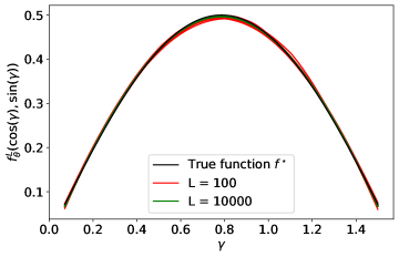
(a) True function and trained MLP after 2000 iterations.

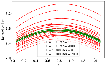
(b) Scaled NTK values

Figure 3: Depth $L$ MLPs learning a toy function with 2D inputs as described in Section 5.1, (Left) Trained deep MLP approximates the true function well, i.e., training succeeds. (Right) Kernel values evaluated at initialization and after training with 10 independent initialization-training trials each for $L=100$ and $L=10000$. As $L$ grows, initialization becomes less random, as Theorem 1 predicts, and the kernel changes less throughout training, as Theorem 2 predicts.

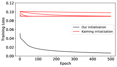
(a) Depth 1000 MLP

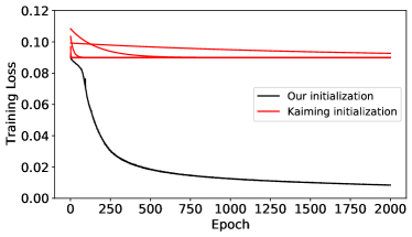
(b) Depth 1000 CNN

Figure 4: Depth 1000 MLPs and CNNs with MNIST are trainable with our proposed initialization but not with the standard Kaiming He initialization. For Kaiming initialization, we show trials with learning rates $1\times 10^{-5}$, $1\times 10^{-4}$, $1\times 10^{-3}$, $0.01$, $0.1$, and $1$.

Task	Architecture	Depth	$C_{L}$	$\rho$	$\beta$	Learning rate	Epochs	Training loss	Test accuracy
10-class	MLP	4000	$4$	1	1	$1\times 10^{-5}$	1500	0.0055	97.48%
10-class	CNN	4000	$4$	$1/\sqrt{3}$	1	$1\times 10^{-5}$	2000	0.014578	94.02%
Binary	CNN	20000	$20$	$1/\sqrt{3}$	1	$1\times 10^{-8}$	1000	0.031257	98.87%

Table 1: Very deep MLP and CNNs trained with MNIST. As the theory predicts, the very deep networks are trainable.

4.2 Convergence in infinite-depth limit

We now analyze the convergence of the infinitely deep CNN.

Theorem 4 (Scaled NTK at initialization).

Suppose $f^{L+1}_{\theta}$ is initialized as in Section 4.1. For any $x,x^{\prime}\in\mathbb{R}_{+}^{d\times d}$,

$$S\left({\tilde{\Theta}^{L}_{0}(x,x^{\prime})}\right)\stackrel{{\scriptstyle p}}{{\rightarrow}}\tilde{\Theta}^{\infty}(x,x^{\prime})$$

as $L\rightarrow\infty$, where

$$\tilde{\Theta}^{\infty}(x,x^{\prime})=\frac{1}{d^{2}}\sum_{s=1}^{3}\sum_{u=1}^{3}\bigg{(}p_{d}(s,u)+d^{2}S(x_{\psi_{s,u}})S(x^{\prime}_{\psi_{s,u}})$$

$$\qquad+\sum_{i,j\in\psi_{s,u}}\sum_{i^{\prime},j^{\prime}\in\psi_{s,u}}\mathbb{E}[\sigma(g(\phi_{i,j}(x)))\sigma(g(\phi_{i^{\prime},j^{\prime}}(x^{\prime})))]\bigg{)},$$

$g\sim\mathcal{GP}(0,\rho^{2}\left\langle x,x^{\prime}\right\rangle+\beta^{2})$, $\psi_{s,u}$ is the set of coordinate which satisfy $x_{\psi_{s,u}}=[x]_{s-1:d+s-2,u-1:d+u-2}$ and $x_{pq}=0,\phi_{mn}(x)=0$ if the index is out of bounds, and

$$p_{d}(s,u)=\left\{\begin{array}[]{ll}d^{4}&(s,u)=(2,2),\\ d^{2}(d-1)^{2}&|s-u|=1,\\ (d-1)^{4}&\text{else}.\end{array}\right.$$

Theorem 5 (Invariance of scaled NTK).

Let $T>0$. Suppose $\int_{0}^{T}\left\|{\delta|_{f_{\theta}^{L}}}\right\|_{p^{in}}\!\!\!\!dt$ is stochastically bounded as $L\rightarrow\infty$. Then, for any $x,x^{\prime}\in\mathbb{R}^{d\times d}_{+}$,

$$S\left({\tilde{\Theta}^{L}_{t}(x,x^{\prime})}\right)\stackrel{{\scriptstyle p}}{{\rightarrow}}\tilde{\Theta}^{\infty}(x,x^{\prime})$$

uniformly for $t\in[0,T]$ as $L\rightarrow\infty$.

Again, define the kernel regression predictor as

$$f_{\mathrm{ntk}}(x)=\left({\tilde{\Theta}^{\infty}(x,x_{1}),\dots,\tilde{\Theta}^{\infty}(x,x_{N})}\right)K^{-1}f^{\star}(X),$$

where $K_{i,j}=\tilde{\Theta}^{\infty}(x_{i},x_{j})$ and $[f^{\star}(X)]_{i}=f^{\star}(x_{i})$ for $i,j\in\{1,\dots,N\}$.

Theorem 6 (Equivalence between deep CNN and kernel regression).

Let $\mathcal{L}(f)=\frac{1}{2}\left\|{f-f^{\star}}\right\|_{p^{in}}^{2}$. Let $\tilde{\Theta}^{\infty}$ be positive definite. If $f_{t}$ follows the kernel gradient flow with respect to $\tilde{\Theta}^{\infty}$, then for any $x\in\mathbb{R}^{d\times d}_{+}$,

$$\lim_{t\rightarrow\infty}f_{t}(x)=f_{\mathrm{ntk}}(x).$$

Generalizations.

At the expense of slight notational complications, we can generalize our results as follows. We assumed the convolutional filter size is $3\times 3$, but we can use larger filters by assigning a symbol for the filter size and managing the summation indices with care. We assumed the number of input channels and output scalar dimension are $1$, but we can have $c$ input channels and $k$ outputs, i.e., $f^{L+1}_{\theta}\colon\mathbb{R}^{c\times d\times d}_{+}\rightarrow\mathbb{R}^{k}$, by letting the intermediate layers have $c+1+k$ channels. In fact, Section 5.2 presents a 10-class classification of MNIST with a deep CNN using $1+1+10=12$ channels in intermediate layers.

5 Experiments

In this section, we experimentally demonstrate the invariance of the scaled NTK and the trainability of deep neural networks. The code is available at https://github.com/lthilnklover/deep-narrow-NTK

5.1 Convergence of the scaled NTK

Our first experiment, inspired by Jacot et al. (2018), trains $L$-layer MLPs on 2-dimensional inputs and shows that the network and its scaled NTK converges as the depth $L$ increases. For $L=100$ and $L=10000$, we initialize 10 independent MLP instances and train them to approximate $f^{\star}(x_{1},x_{2})=x_{1}x_{2}$ using the quadratic loss. To verify that the networks are indeed successfully trained, we compare the trained MLP against the true function $f^{\star}$ in Figure 3(a). We then plot the scaled NTK $\tilde{\Theta}^{L}(x_{0},x)$ for fixed $x_{0}=\big{(}\frac{1}{\sqrt{2}},\frac{1}{\sqrt{2}}\big{)}$ and $x=(\cos(\gamma),\sin(\gamma))$ for $0<\gamma<\pi/2$ in Figure 3(b). The kernels are plotted at initialization ($t=0$), and after 2000 iterations of gradient descent.

5.2 Trainability of the deep narrow neural network

Next, we demonstrate the empirical trainability of the deep narrow networks on the MNIST dataset.

Very deep MLP.

We train $L$-layer MLPs with $d_{\mathrm{in}}=784$ and $d_{\mathrm{out}}=10$ using the quadratic loss with one-hot vectors as targets. To establish a point of comparison, we attempt to train a 1000-layer MLP with the typical Kaiming He uniform initialization (He et al., 2015). We tuned the learning rate via a grid search from $0.00001$ to $1.0$, but the network was untrainable, as one would expect based on the prior findings of (He & Sun, 2015; Srivastava et al., 2015; Huang et al., 2020). In contrast, when we use the initialization defined in Section 3.1, the deep MLP was trainable. Figure 4(a) reports these results. To push the depth, we also trained a 4000-layer MLP and report the results in Table 1. To the best of our knowledge, this 4000-layer MLP holds the record for the deepest trained MLP.

Very deep CNN.

We train $L$-layer CNNs using the quadratic loss with one-hot probability vectors as targets. To reduce the computational cost, we insert a $4\times 4$ average pool before the first layer to reduce the MNIST input size to $7\times 7$. As in the MLP experiment, we attempt to train a 1000-layer CNN with the typical Kaiming He uniform initialization, but the network was untrainable. In contrast, when we use the initialization defined in Section 4.1, the deep CNN was trainable. Figure 4(b) reports these results. To push the depth, we also trained a 4000-layer CNN and report the results in Table 1. To further push the depth, we simplify the problem to binary classification between digits 0 and 1 and use values $0$ and $1$ as targets. We then trained a 20000-layer CNN and report the results in Table 1. This CNN surpasses the 10000-depth CNN of (Xiao et al., 2018) and, to the best of our knowledge, holds the record of the deepest trained CNN.

5.3 Accumulation of the layer-wise effect

To observe the accumulation of the output value throughout the depth, we plot the intermediate activation values of the rightmost neurons of each layer from the $10000$-layer MLP trained in Section 5.1. Precisely, we plot $(\sigma(f^{(l)}(x)))_{d_{\mathrm{in}}+d_{\mathrm{out}}+1}-C_{L}$ for $1\leq l\leq L-1$ and $(f^{(L)}(x))_{d_{\mathrm{in}}+d_{\mathrm{out}}+1}$. Figure 5 shows that the target output value is achieved through the accumulation of the effect of $10000$-layers.

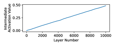
Figure 5: Intermediate activation values of the rightmost neurons of each layer after training. (The effect of the bias $C_{L}$ is compensated for to help visualize the change.)

6 Conclusion

This work presents an NTK analysis of a deep narrow MLP and CNN in the infinite-depth limit and establishes the first trainability guarantee on deep narrow neural networks. Our results serve as a demonstration that infinitely deep neural networks can be made provably trainable using the right initialization, just as the infinitely wide counterparts are. However, our results do have the following limitations. First, while our proposed initialization is straightforwardly implementable, it is far from the initializations used in practice. Second, our results do not indicate any benefit of using deep neural networks compared to wide neural networks. Further investigating the trainability of overparameterized deep neural networks to address these questions would be an interesting direction of future work.

Appendix A Preliminaries

A.1 Grönwall’s lemma

The following is a generalized version of Grönwall’s lemma, which is essential to prove the invariance of kernel.

Lemma 7 (Dragomir 2003).

Let the $x,a,b$ and $k$ be continuous and nonnegative functions on $J=[\alpha,\beta]$. Let $n\geq 2$ be a positive integer $\frac{a}{b}$ be a nondecreasing function. If

$$z(t)\leq a(t)+b(t)\int_{\alpha}^{t}k(s)z^{n}(s)\,ds,\,\,t\in J$$

then

$$z(t)\leq a(t)\left\{1-(n-1)\int_{\alpha}^{t}k(s)b(s)a^{n-1}(s)\,ds\right\}^{\frac{1}{1-n}},$$

where $\alpha\leq t\leq\beta_{n}$, for $\beta_{n}$ defined by

$$\beta_{n}=\mathrm{sup}\left\{t\in J:(n-1)\int_{\alpha}^{t}kba^{n-1}\,ds<1\right\}.$$

Appendix B Proof of Theorems of NTK for MLP

B.1 Proof of Theorem 1

The following lemma shows the recursive relation of the neural tangent kernel (without the scaling factor).

Lemma 8.

For $t\geq 0$, $l\geq 2$ and $x,x^{\prime}\in\mathbb{R}_{+}^{d_{in}}$,

$$\Theta^{l}_{t}(x,x^{\prime}) =W^{l}(t)\mbox{diag}(\dot{\sigma}(f^{l-1}_{\theta^{(l-1)}}(x)))\Theta^{l-1}_{t}(x,x^{\prime})\mbox{diag}(\dot{\sigma}(f^{l-1}_{\theta^{(l-1)}(t)}(x^{\prime})))(W^{l}(t))^{\intercal}$$

$$\quad+(\sigma(f^{l-1}_{\theta^{(l-1)}(t)}(x^{\prime}))^{\intercal}\sigma(f^{l-1}_{\theta^{(l-1)}(t)}(x))+1)I_{d_{\mathrm{in}}+d_{\mathrm{out}}+1},$$

where $\Theta^{1}_{t}(x,x^{\prime})=(x^{\intercal}x^{\prime}+1)I_{d_{\mathrm{in}}+d_{\mathrm{out}}+1}$ if $l=1$.

Proof of Lemma 8.

$$\Theta^{l}_{t}(x,x^{\prime}) =\partial_{\theta^{(l)}}f^{l}_{\theta^{(l)}(t)}(x)\left({\partial_{\theta^{(l)}}f^{l}_{\theta^{(l)}(t)}(x^{\prime})}\right)^{\intercal}$$

$$=\sum_{\theta_{i}\in\theta^{(l)}}\partial_{\theta_{i}}f^{l}_{\theta^{(l)}(t)}(x)\left({\partial_{\theta_{i}}f^{l}_{\theta^{(l)}(t)}(x^{\prime})}\right)^{\intercal}$$

$$=\sum_{\theta_{i}\in\theta^{(l-1)}}\partial_{\theta_{i}}f^{l}_{\theta^{(l)}(t)}(x)\left({\partial_{\theta_{i}}f^{l}_{\theta^{(l)}(t)}(x^{\prime})}\right)^{\intercal}$$

$$\quad+\sum_{W^{l}_{ij}}\partial_{W^{l}_{ij}}f^{l}_{\theta^{(l)}(t)}(x)\left({\partial_{W^{l}_{ij}}f^{l}_{\theta^{(l)}(t)}(x^{\prime})}\right)^{\intercal}+\sum_{b^{l}_{i}}\partial_{b^{l}_{i}}f^{l}_{\theta^{(l)}(t)}(x)\left({\partial_{b^{l}_{i}}f^{l}_{\theta^{(l)}(t)}(x^{\prime})}\right)^{\intercal}.$$

The last two terms of RHS is

$$\sum_{W^{l}_{ij}}\left({\partial_{W^{l}_{ij}}f^{l}_{\theta^{(l)}(t)}(x)}\right)_{k}\left({\partial_{W^{l}_{ij}}f^{l}_{\theta^{(l)}(t)}(x^{\prime})}\right)_{k^{\prime}}+\sum_{b^{l}_{i}}\left({\partial_{b^{l}_{i}}f^{l}_{\theta^{(l)}(t)}(x)}\right)_{k}\left({\partial_{b^{l}_{i}}f^{l}_{\theta^{(l)}(t)}(x^{\prime})}\right)_{k^{\prime}}$$

$$=(\sigma(f^{l-1}_{\theta^{(l-1)}(t)}(x))^{\intercal}\sigma(f^{l-1}_{\theta^{(l-1)}(t)}(x^{\prime}))+1)\delta_{k,k^{\prime}},$$

where $(\cdot)_{k}$ denote the $k$-th component of the vector, and $\delta_{k,k^{\prime}}=1$ if $k=k^{\prime}$ and $0$ otherwise. Also, since

$$\partial_{\theta^{(l-1)}}f^{l}_{\theta^{(l)}(t)}(x)=W^{l}(t)\mbox{diag}(\dot{\sigma}(f^{l-1}_{\theta^{(l-1)}(t)}(x)))\partial_{\theta^{(l-1)}}f^{l-1}_{\theta^{(l-1)}(t)}(x),$$

the first term of RHS is

$$\sum_{\theta_{i}\in\theta^{(l-1)}}\partial_{\theta_{i}}f^{l}_{\theta^{(l)}(t)}(x)\left({\partial_{\theta_{i}}f^{l}_{\theta^{(l)}(t)}(x^{\prime})}\right)^{\intercal}= \partial_{\theta^{(l-1)}}f^{l}_{\theta^{(l)}(t)}(x)\left({\partial_{\theta^{(l-1)}}f^{l}_{\theta^{(l)}(t)}(x^{\prime})}\right)^{\intercal}$$

$$= W^{l}(t)\mbox{diag}(\dot{\sigma}(f^{l-1}_{\theta^{(l-1)}(t)}(x)))\Theta^{l-1}_{t}(x,x^{\prime})\mbox{diag}(\dot{\sigma}(f^{l-1}_{\theta^{(l-1)}(t)}(x^{\prime})))(W^{l}(t))^{\intercal}.$$

Thus, we have a recursive relation for kernel

$$\Theta^{l}_{t}(x,x^{\prime}) =W^{l}(t)\mbox{diag}(\dot{\sigma}(f^{l-1}_{\theta^{(l-1)}}(x)))\Theta^{l-1}_{t}(x,x^{\prime})\mbox{diag}(\dot{\sigma}(f^{l-1}_{\theta^{(l-1)}(t)}(x^{\prime})))(W^{l}(t))^{\intercal}$$

$$\quad+(\sigma(f^{l-1}_{\theta^{(l-1)}(t)}(x))^{\intercal}\sigma(f^{l-1}_{\theta^{(l-1)}(t)}(x^{\prime}))+1)I_{d_{\mathrm{in}}+d_{\mathrm{out}}+1}.$$

for $l\geq 2$, where $\Theta^{1}_{t}(x,x^{\prime})=(x^{\intercal}x^{\prime}+1)I_{d_{\mathrm{in}}+d_{\mathrm{out}}+1}$ if $l=1$. ∎

For notational simplicity, we let

$$\mathfrak{W}^{k}_{j}(x,t)=W^{j}(t)\mbox{diag}\left(\dot{\sigma}\left(f^{j-1}_{\theta^{(j-1)}(t)}(x)\right)\right)W^{j-1}(t)\mbox{diag}\left(\dot{\sigma}\left(f^{j-2}_{\theta^{(j-2)}(t)}(x)\right)\right)\cdots W^{k}(t)\mbox{diag}\left(\dot{\sigma}\left(f^{k-1}_{\theta^{(k-1)}(t)}(x)\right)\right)$$

for $2\leq k,j\leq L$, where $\mathfrak{W}^{k}_{j}(x,t)=1$ if $k>j$. By applying the above recursive relation inductively, we get the following corollary.

Corollary 9.

For any $x,x^{\prime}\in\mathbb{R}_{+}^{d_{in}}$, and $t\geq 0$,

$$\tilde{\Theta}^{L}_{t}(x,x^{\prime}) =\frac{1}{L}\sum_{l=0}^{L-1}\left[\left(\frac{1}{C_{L}}\sigma\left(f^{l}_{\theta^{(l)}(t)}(x)\right)^{\intercal}\frac{1}{C_{L}}\sigma\left(f^{l}_{\theta^{(l)}(t)}(x^{\prime})\right)\right)\mathfrak{W}_{L}^{l+2}(x,t)\mathfrak{W}_{L}^{l+2}(x^{\prime},t)^{\intercal}\right]$$

$$\quad+\frac{1}{LC_{L}^{2}}\sum_{l=0}^{L-1}\left[\mathfrak{W}_{L}^{l+2}(x,t)\mathfrak{W}_{L}^{l+2}(x^{\prime},t)^{\intercal}\right],$$

where we define $\sigma(f^{0}(x))=x$ for convenience.

Now, we are ready to prove the Theorem 1.

Proof of Theorem 1.

At initialization, we can simplify the kernel further. Since we assumed positive input, we have

$$W^{l}(0)\mbox{diag}(\dot{\sigma}(f^{l-1}_{\theta^{(l-1)}(0)}(x)))= \begin{bmatrix}I_{d_{\mathrm{in}}}&0_{d_{\mathrm{in}}\times 1}&0_{d_{\mathrm{in}}\times d_{\mathrm{out}}}\\ u^{l}&0_{1\times 1}&0_{1\times d_{\mathrm{out}}}\\ 0_{d_{\mathrm{out}}\times d_{\mathrm{in}}}&0_{d_{\mathrm{out}}\times 1}&I_{d_{\mathrm{out}}}\end{bmatrix}\quad\mbox{for $1\leq l\leq L-1$,}$$

$$W^{L}(0)\mbox{diag}(\dot{\sigma}(f^{L-1}_{\theta^{(L-1)}(0)}(x)))= \begin{bmatrix}0_{d_{\mathrm{out}}\times d_{\mathrm{in}}}&0_{d_{\mathrm{out}}\times 1}&I_{d_{\mathrm{out}}}\end{bmatrix}.$$

This implies

$$\mathfrak{W}^{k}_{l}(x,0)=W^{l}(0)\mbox{diag}(\dot{\sigma}(f^{l-1}_{\theta^{(l-1)}(0)}))=W^{l}(0)$$ (1)

for $l\geq k$. Also, our initialization implies

$$f^{1}_{\theta^{(1)}(0)}(x)=\begin{bmatrix}C_{L}x\\ (u^{1})^{\intercal}x+v^{1}\\ C_{L}\mathbbm{1}_{d_{\mathrm{out}}}\end{bmatrix},\,\,f^{l}_{\theta^{(l)}(0)}(x)=\begin{bmatrix}C_{L}x\\ C_{L}(u^{l})^{\intercal}x+v^{l}\\ C_{L}\mathbbm{1}_{d_{\mathrm{out}}}\end{bmatrix},\,\,f^{L}_{\theta^{(L)}(0)}=0_{d_{\mathrm{in}}\times 1}$$ (2)

for $2\leq l\leq L-1$. Thus, the scaled NTK is given by

$$\tilde{\Theta}^{L}_{0}(x,x^{\prime})=\frac{1}{LC_{L}^{2}}\left({x^{\intercal}x^{\prime}+1+\sum_{j=0}^{L-1}(C_{L}^{2}x^{\intercal}x^{\prime}+\sigma(C_{L}(u^{j})^{\intercal}x+v^{j})\sigma(C_{L}(u^{j})^{\intercal}x^{\prime}+v^{j})+C_{L}^{2}+1)}\right)I_{d_{\mathrm{out}}}.$$

Let $g^{j}(x)=u^{j}x+v^{j}/C_{L}$, then $\{g^{j}(x)\}_{j=0}^{L-1}$ are i.i.d. Gaussian process, where $g^{j}\sim\mathcal{GP}(0,\frac{\rho^{2}}{d_{in}}x^{\intercal}x^{\prime}+\beta^{2})$. This is because

$$\mathbb{E}_{u^{j},v^{j}}[g^{j}]=0$$

and

$$\mathbb{E}_{u^{j},v^{j}}[g^{j}(x)g^{j}(x^{\prime})] =\mathbb{E}_{u^{j},v^{j}}\left[\left((u^{j})^{\intercal}x+v^{j}/C_{L}\right)\left((u^{j})^{\intercal}x^{\prime}+v^{j}/C_{L}\right)\right]$$

$$=\mathbb{E}_{u^{j}}\left[\left((u^{j})^{\intercal}x\right)\left((u^{j})^{\intercal}x^{\prime}\right)\right]+\beta^{2}$$

$$=\frac{\rho^{2}}{d}x^{\intercal}x^{\prime}+\beta^{2}.$$

Hence, we have

$$\tilde{\Theta}^{L}_{0}(x,x^{\prime})\stackrel{{\scriptstyle p}}{{\rightarrow}}\left({x^{\intercal}x^{\prime}+1+\mathbb{E}_{g\sim\mathcal{GP}(0,\frac{\rho^{2}}{d_{\mathrm{in}}}x^{\intercal}x^{\prime}+\beta^{2})}[\sigma(g(x))\sigma(g(x^{\prime}))]}\right)I_{d_{\mathrm{out}}}$$

as $L\rightarrow\infty$ by the law of large number, which concludes the proof. ∎

B.2 Proof of Theorem 2

For proving our scaled NTK stays constant during training, we need to show that intermediate weight and pre-activation values are effectively unchanged. In this paper, we also consider Lyapunov functions similar to (Jacot et al., 2018); however, we need more delicate Lyapunov function to handle infinite depth network.

For the sake of simplicity, we set the scaling factor of gradient flow by $\frac{1}{(L-1)C_{L}^{2}}$ throughout the proof. Also, without loss of generality, we assume the norms of data points $\left\|{x_{i}}\right\|$ are bounded by 1 for all $1\leq i\leq N$, and we further assume that all other inputs $x\notin\{x_{1},\dots,x_{N}\}$ also have bounded norm, i.e., $\left\|{x}\right\|\leq 1$.

We define Lyapunov functions to track intermediate weights and pre-activation values of the network. For $1\leq j\leq 8$ and $C_{L}>0$ satisfying $L^{2}/C_{L}\rightarrow 0$,

$$\Phi_{L,j}(t) =\frac{1}{(L-1)C_{L}^{j}}\sum^{L-1}_{l=1}\left(\left\|{f^{l}_{\theta^{(l)}(0)}(x)}\right\|_{p^{in}}+\left\|{f^{l}_{\theta^{(l)}(t)}(x)-f^{l}_{\theta^{(l)}(0)}(x)}\right\|_{p^{in}}\right)^{j}$$

$$\Psi_{L,2}(t) =\frac{1}{(L-1)^{2}}\sum^{L}_{l=2}\frac{L-1}{l-1}\sum_{i=2}^{l}\left(\left\|{\mathfrak{W}_{l}^{i}(x,0)}\right\|_{p^{in}}+\left\|{\mathfrak{W}_{l}^{i}(x,t)-\mathfrak{W}_{l}^{i}(x,0)}\right\|_{p^{in}}\right)^{2}$$

$$\Psi_{L,8}(t) =\frac{1}{L-1}\sum_{l=2}^{L}\left(\left\|{\mathfrak{W}_{L}^{l}(x,0)}\right\|_{p^{in}}+\left\|{\mathfrak{W}_{L}^{l}(x,t)-\mathfrak{W}_{L}^{l}(x,0)}\right\|_{p^{in}}\right)^{8},$$

where $\Phi_{L,0}=1$.

At initialization ($t=0$), we have

$$\Phi_{L,j}(0) =\frac{1}{(L-1)C_{L}^{j}}\sum^{L-1}_{l=1}\left(\left\|{f^{l}_{\theta^{(l)}(0)}(x)}\right\|_{p^{in}}\right)^{j}$$

$$\Psi_{L,2}(0) =\frac{1}{(L-1)^{2}}\sum^{L}_{l=2}\frac{L-1}{l-1}\sum_{i=2}^{l}\left(\left\|{\mathfrak{W}_{l}^{i}(x,0)}\right\|_{p^{in}}\right)^{2}$$

$$\Psi_{L,8}(0) =\frac{1}{L-1}\sum_{l=2}^{L}\left(\left\|{\mathfrak{W}_{L}^{l}(x,0)}\right\|_{p^{in}}\right)^{8}.$$

From (1) and (2), imply that $\Phi_{L,j}(0)$ and $\Psi_{L,2}(0)$ converges (in probability) to constant values $\Phi_{\infty,j}(0)$ and $\Psi_{\infty,2}(0)$ by the law of large number, respectively. Furthermore, $\Psi_{L,8}(0)$ also converges (in probability) to constant value $\Psi_{\infty,8}(0)$ since $\mathfrak{W}_{L}^{l}(x,0)=W^{L}(0)$. Then, the following proposition implies Lyapunov function remains constant during training.

Proposition 1.

For $1\leq j\leq 8$,

$$\Phi_{L,j}(t)\stackrel{{\scriptstyle p}}{{\rightarrow}}\Phi_{\infty,j}(0),\quad\Psi_{L,2}(t)\stackrel{{\scriptstyle p}}{{\rightarrow}}\Psi_{\infty,2}(0),\quad\Psi_{L,8}(t)\stackrel{{\scriptstyle p}}{{\rightarrow}}\Psi_{\infty,8}(0)$$

uniformly for $t\in[0,T]$ as $L\rightarrow\infty$.

The following lemma is a key step to prove the proposition which allows us to apply Grönwall’s Lemma. For the sake of simplicity, we let $\delta_{t}^{L}=\partial_{f}C=\delta|_{f_{\theta}^{L}}$.

Lemma 10.

For $t\geq 0$, if $f^{l}_{\theta^{(l)}(t)}(x)$ is element-wise nonzero for $1\leq l\leq L-1$ and $x\in\{x_{1},\dots,x_{N}\}$, then

$$\partial_{t}\Phi_{L,j}(t) \leq\frac{2jN^{3/2}(L-1)}{C_{L}}\Phi_{L,j-1}(t)\Phi_{L,8}(t)\Psi_{L,2}(t)\Psi_{L,8}(t)\left\|{\delta^{L}_{t}}\right\|_{p^{in}}$$

$$\partial_{t}\Psi_{L,2}(t) \leq\frac{2N(L-1)}{C_{L}}\Phi_{L,4}(t)\left({\Psi_{L,2}(t)}\right)^{2}(t)\Psi_{L,8}(t)\left\|{\delta^{L}_{t}}\right\|_{p^{in}}$$

$$\partial_{t}\Psi_{L,8}(t) \leq\frac{8N(L-1)}{C_{L}}\Phi_{L,4}(t)\Psi_{L,2}(t)\left(\Psi_{L,8}(t)\right)^{2}\left\|{\delta^{L}_{t}}\right\|_{p^{in}},$$

for $1\leq j\leq 8$.

The proof of Lemma 10 is given in Section F.

Proof of Proposition 1.

In order to apply Lemma 10 for all $t\in[0,T]$, we need to show that $f^{l}_{\theta^{(l)}(t)}(x)$ is element-wise nonzero for all $t\in[0,T]$, $1\leq l\leq L-1$, and $x\in\{x_{1},\dots,x_{N}\}$. This is indeed true when $L$ is large enough, which we proved in Section C. From Lemma 10, we get

$$\partial_{t}\left(\sum_{j=1}^{8}\Phi_{L,j}(t)+\Psi_{L,2}(t)+\Psi_{L,8}(t)\right) \leq\frac{16N^{3/2}(L-1)}{C_{L}}\left(\sum_{j=1}^{8}\Phi_{L,j}(t)+\Psi_{L,2}(t)+\Psi_{L,8}(t)\right)^{4}\left\|{\delta^{L}_{t}}\right\|_{p^{in}},$$

which implies

$$\Gamma_{L}(t) \leq\Gamma_{L}(0)+\frac{16N^{3/2}(L-1)}{C_{L}}\int_{0}^{t}\Gamma_{L}(s)^{4}\left\|{\delta_{s}^{L}}\right\|_{p^{in}}\,ds,$$

where $\Gamma_{L}(t)=\sum_{j=1}^{8}\Phi_{L,j}(t)+\Psi_{L,2}(t)+\Psi_{L,8}(t)$. By Grönwall’s lemma with $z(t)=\Gamma_{L}(t),\,a(t)=\Gamma_{L}(0),\,b(t)=\frac{16N^{3/2}(L-1)}{C_{L}},\,k(s)=\left\|{\delta^{L}_{s}}\right\|_{p^{in}}$,

$$\Gamma_{L}(t)\leq\Gamma_{L}(0)\left\{1-\frac{48N^{3/2}(L-1)}{C_{L}}\Gamma_{L}(0)^{3}\int_{0}^{t}\left\|{\delta^{L}_{s}}\right\|_{p^{in}}\,ds\right\}^{-\frac{1}{3}}$$

for $0\leq t\leq\beta_{L}$. Recall that $\int_{0}^{T}\left\|{\delta_{s}^{L}}\right\|_{p^{in}}\,ds$ is stochastically bounded and $\Gamma_{L}(0)$ converges to a constant. Thus, for $L^{2}/C_{L}\rightarrow 0$, we get $\frac{48N^{3/2}(L-1)}{C_{L}}\Gamma_{L}(0)^{3}\int_{0}^{t}\left\|{\delta^{L}_{s}}\right\|_{p^{in}}\,ds\stackrel{{\scriptstyle p}}{{\rightarrow}}0$. This implies the upper bound of $\Gamma_{\infty}(t)$ converges to $\Gamma_{\infty}(0)$ in probability. On the other hand, $\Gamma_{L}(t)\geq\Gamma_{L}(0)$ by construction and $\beta_{L}\rightarrow\infty$ as $L\rightarrow\infty$. Thus, $\Gamma_{L}(t)\stackrel{{\scriptstyle p}}{{\rightarrow}}\Gamma_{\infty}(0)$ uniformly for $t\in[0,T]$. This concludes the proof. ∎

Next, we consider similar Lyapunov functions but under $\ell_{2}$ norm. This is because scaled NTK is not restricted to the dataset. For $1\leq j\leq 8$,

$$\tilde{\Phi}_{L,j}(x,t) =\frac{1}{(L-1)C_{L}^{j}}\sum^{L-1}_{l=1}\left(\left\|{f^{l}_{\theta^{(l)}(0)}(x)}\right\|+\left\|{f^{l}_{\theta^{(l)}(t)}(x)-f^{l}_{\theta^{(l)}(0)}(x)}\right\|\right)^{j}$$

$$\tilde{\Psi}_{L,2}(x,t) =\frac{1}{(L-1)^{2}}\sum^{L}_{l=2}\frac{L-1}{l-1}\sum_{i=2}^{l}\left(\left\|{\mathfrak{W}_{l}^{i}(x,0)}\right\|+\left\|{\mathfrak{W}_{l}^{i}(x,t)-\mathfrak{W}_{l}^{i}(x,0)}\right\|\right)^{2}$$

$$\tilde{\Psi}_{L,8}(x,t) =\frac{1}{L-1}\sum_{l=2}^{L}\left(\left\|{\mathfrak{W}_{L}^{l}(x,0)}\right\|+\left\|{\mathfrak{W}_{L}^{l}(x,t)-\mathfrak{W}_{L}^{l}(x,0)}\right\|\right)^{8},$$

where $\tilde{\Phi}_{L,0}=1$.

Note that Lyapunov functions under $\ell_{2}$-norm are functions of $(x,t)$. Similar to Lyapunov functions under $p^{in}$-norm, at initialization ($t=0$), we have $\tilde{\Phi}_{L,j}(x,0)\stackrel{{\scriptstyle p}}{{\rightarrow}}\tilde{\Phi}_{\infty,j}(x,0),\,\tilde{\Psi}_{L,2}(x,0)\stackrel{{\scriptstyle p}}{{\rightarrow}}\tilde{\Psi}_{\infty,2}(x,0),\,\tilde{\Psi}_{L,8}(x,0)\stackrel{{\scriptstyle p}}{{\rightarrow}}\tilde{\Psi}_{\infty,8}(x,0)$, where $\tilde{\Phi}_{L,\infty}(x,0),\tilde{\Psi}_{\infty,2}(x,0),\tilde{\Psi}_{\infty,8}(x,0)$ are constant by the law of large number. The similar proposition holds, which implies the intermediate weights and pre-activation values are invariant during training in $\ell_{2}$-norm sense.

Proposition 2.

For $1\leq j\leq 8$ and any $T>0$,

$$\tilde{\Phi}_{L,j}(x,t)\stackrel{{\scriptstyle p}}{{\rightarrow}}\tilde{\Phi}_{\infty,j}(x,0),\quad\tilde{\Psi}_{L,2}(x,t)\stackrel{{\scriptstyle p}}{{\rightarrow}}\tilde{\Psi}_{\infty,2}(x,0),\quad\tilde{\Psi}_{L,8}(x,t)\stackrel{{\scriptstyle p}}{{\rightarrow}}\tilde{\Psi}_{\infty,8}(x,0)$$

uniformly for $t\in[0,T]$ as $L\rightarrow\infty$.

The following lemma, which corresponds to Lemma 10, allows us to apply Grönwall’s lemma.

Lemma 11.

For $t\geq 0$ and $x\in\mathbb{R}_{+}^{d_{in}}$, if $f^{l}_{\theta^{(l)}(t)}(x)$ is element-wise nonzero for $1\leq l\leq L-1$, then

$$\partial_{t}\tilde{\Psi}_{L,2}(x,t) \leq\frac{2(L-1)}{C_{L}}\left({\tilde{\Psi}_{L,2}(x,t)}\right)^{2}\Phi_{L,4}(t)\Psi_{L,8}(t)\left\|{\delta^{L}_{t}}\right\|_{p^{in}}$$

$$\partial_{t}\tilde{\Phi}_{L,j}(x,t) \leq\frac{2jN^{1/2}(L-1)}{C_{L}}\tilde{\Phi}_{L,j-1}(t)\tilde{\Phi}_{L,8}(x,t)\tilde{\Psi}_{L,2}(x,t)\Phi_{L,8}(t)\Psi_{L,8}(t)\left\|{\delta^{L}_{t}}\right\|_{p^{in}}$$

$$\partial_{t}\tilde{\Psi}_{L,8}(x,t) \leq\frac{8(L-1)}{C_{L}}\tilde{\Phi}_{L,4}(x,t)\tilde{\Psi}_{L,2}(x,t)\left({\tilde{\Psi}_{L,8}(x,t)}\right)^{2}\Psi_{L,8}(t)\left\|{\delta^{L}_{t}}\right\|_{p^{in}},$$

for $1\leq j\leq 8$.

The proof of Lemma 11 is given in Section G.

Proof of Proposition 2.

Similar to the proof of Proposition 1, we need to show that $f^{l}_{\theta^{(l)}(t)}(x)$ is element-wise nonzero for all $t\in[0,T]$, $1\leq l\leq L-1$, and $x\in\mathbb{R}_{+}^{d_{in}}$. Again, the element-wise nonzero assumption also holds if $L$ is large enough, and the proof is given in Section C. From Lemma 11,

$$\tilde{\Psi}_{L,2}(x,t)\leq\tilde{\Psi}_{L,2}(x,0)+\frac{2(L-1)}{C_{L}}\int^{t}_{0}{\left({\tilde{\Psi}_{L,2}(x,s)}\right)^{2}\Phi_{L,4}(s)\Psi_{L,8}(s)\left\|{\delta^{L}_{s}}\right\|_{p^{in}}\,ds.}$$

Then using Grönwall’s lemma where $z(t)=\tilde{\Psi}_{L,2}(x,t),\,a(t)=\tilde{\Psi}_{L,2}(x,0),\,b(t)=\frac{2(L-1)}{C_{L}},\,k(s)=\Phi_{L,4}(s)\Psi_{L,8}(s)\left\|{\delta^{L}_{s}}\right\|_{p^{in}}$, we get

$$\tilde{\Psi}_{L,2}(x,t)\leq\tilde{\Psi}_{L,2}(x,0)\left\{1-\frac{2(L-1)}{C_{L}}\tilde{\Psi}_{L,2}(x,0)\int^{t}_{0}\Phi_{L,4}(s)\Psi_{L,8}(s)\left\|{\delta^{L}_{s}}\right\|_{p^{in}}\,ds\right\}^{-1}$$

for all $0\leq t\leq\beta_{L}$. Similar to the proof of Proposition 1, if $L^{2}/C_{L}\rightarrow 0$, then we get $\tilde{\Psi}_{L,2}(t)\stackrel{{\scriptstyle p}}{{\rightarrow}}\tilde{\Psi}_{\infty,2}(0)$ uniformly for $t\in[0,T]$.

On the other hand, Lemma 11 also implies

$$\sum^{8}_{j=1}\tilde{\Phi}_{L,j}(x,t) \leq\sum^{8}_{j=1}\tilde{\Phi}_{L,j}(x,0)+\int^{t}_{0}{\frac{16N^{1/2}(L-1)}{C_{L}}\left({\sum^{8}_{j=1}\tilde{\Phi}_{L,j-1}(x,s)}\right)\tilde{\Phi}_{L,8}(x,s)\tilde{\Psi}_{L,2}(x,s)\Phi_{L,8}(s)\Psi_{L,8}(s)\left\|{\delta^{L}_{s}}\right\|_{p^{in}}\,ds}$$

$$\leq\sum^{8}_{j=1}\tilde{\Phi}_{L,j}(x,0)+\int^{t}_{0}{\frac{16N^{1/2}(L-1)}{C_{L}}\left({\sum^{8}_{j=1}\tilde{\Phi}_{L,j}(x,s)}\right)^{2}\tilde{\Psi}_{L,2}(x,s)\Phi_{L,8}(s)\Psi_{L,8}(s)\left\|{\delta^{L}_{s}}\right\|_{p^{in}}\,ds}$$

$$\tilde{\Psi}_{L,8}(x,t) \leq\tilde{\Psi}_{L,8}(x,0)+\int^{t}_{0}{\frac{8(L-1)}{C_{L}}\left({\tilde{\Psi}_{L,8}(x,s)}\right)^{2}\tilde{\Phi}_{L,4}(x,s)\tilde{\Psi}_{L,2}(x,s)\Psi_{L,8}(s)\left\|{\delta^{L}_{s}}\right\|_{p^{in}}\,ds}.$$

We can similarly apply Grönwall’s lemma to show that $\sum_{j=1}^{8}\tilde{\Phi}_{L,j}(x,t)$ and $\tilde{\Psi}_{L,8}(x,t)$ converge to constant values. ∎

Now, we consider our last and core Lyapunov function which contains intermediate weight and pre-activation values from a single layer. Define

$$\tilde{\Psi}_{L}^{k}(x,t) =\left\|{\mathfrak{W}_{L}^{k}(x,0)}\right\|+\left\|{\mathfrak{W}_{L}^{k}(x,t)-\mathfrak{W}_{L}^{k}(x,0)}\right\|$$

$$\tilde{\Phi}_{L}^{l}(x,t) =\frac{1}{C_{L}}\left({\left\|{f^{l}_{\theta^{(l)}(0)}(x)}\right\|+\left\|{f^{l}_{\theta^{(l)}(t)}(x)-f^{l}_{\theta^{(l)}(0)}(x)}\right\|}\right)$$

for $1\leq l\leq L$ and $2\leq k\leq L$.

At initialization, $\tilde{\Psi}^{k}_{L}(x,0)$ and $\tilde{\Phi}_{L}^{l}(x,0)$ are stochastically bounded. Then the following proposition implies the invariance of Lyapunov functions during training.

Proposition 3.

For $1\leq l\leq L$, $2\leq k\leq L$ and any $T>0$,

$$\tilde{\Psi}^{k}_{L}(x,t)\stackrel{{\scriptstyle p}}{{\rightarrow}}\tilde{\Psi}^{k}_{\infty}(x,0)\quad\tilde{\Phi}^{l}_{L}(x,t)\stackrel{{\scriptstyle p}}{{\rightarrow}}\tilde{\Phi}^{l}_{\infty}(x,0).$$

uniformly for $t\in[0,T]$ as $L\rightarrow\infty$.

This implies individual intermediate weights and pre-activation values are effectively unchanged at each layer. Recall that this layer-wise invariance is straightforward in an infinite width network with finite depth. However, in our setting, an infinitely deep network has composition of infinitely many weights, which requires much careful analysis including the following lemma as well as previous propositions.

Lemma 12.

For $t\geq 0$ and $x\in\mathbb{R}_{+}^{d_{in}}$, if $f^{l}_{\theta^{(l)}(t)}(x)$ is element-wise nonzero for $1\leq l\leq L-1$, then

$$\partial_{t}\tilde{\Psi}^{k}_{L}(x,t) \leq\frac{L-1}{C_{L}}\Psi_{L,8}(t)\tilde{\Phi}_{L,4}(x,t)\tilde{\Psi}_{L,2}(x,t)\tilde{\Psi}_{L,8}(x,t)\left\|{\delta^{L}_{t}}\right\|_{p^{in}}$$

$$\partial_{t}\tilde{\Phi}^{l}_{L}(x,t) \leq\frac{2N^{1/2}(L-1)}{C_{L}}\Phi_{L,8}(t)\Psi_{L,8}(t)\tilde{\Phi}_{L,8}(x,t)\tilde{\Psi}_{L,2}(x,t)\left\|{\delta^{L}_{t}}\right\|_{p^{in}},$$

for $1\leq l\leq L$ and $2\leq k\leq L$.

The proof of Lemma 12 is given in Section H.

Proof of Proposition 3.

As we discussed in the proof of Proposition 2, if $L$ is large enough, $f^{l}_{\theta^{(l)}(t)}(x)$ is element-wise nonzero for all $t\in[0,T]$, $1\leq l\leq L-1$, and $x\in\mathbb{R}_{+}^{d_{in}}$. Lemma 12 implies

$$\tilde{\Psi}^{k}_{L}(x,t) \leq\tilde{\Psi}^{k}_{L}(x,0)+\int^{t}_{0}{\frac{L-1}{C_{L}}\Psi_{L,8}(t)\tilde{\Phi}_{L,4}(x,t)\tilde{\Psi}_{L,2}(x,t)\tilde{\Psi}_{L,8}(x,t)\left\|{\delta^{L}_{t}}\right\|_{p^{in}}\,ds}$$

$$\tilde{\Phi}^{l}_{L}(x,t) \leq\tilde{\Phi}^{l}_{L}(x,0)+\int_{0}^{t}\frac{2N^{1/2}(L-1)}{C_{L}}\Phi_{L,8}(t)\Psi_{L,8}(t)\tilde{\Phi}_{L,8}(x,t)\tilde{\Psi}_{L,2}(x,t)\left\|{\delta^{L}_{t}}\right\|_{p^{in}}\,ds.$$

Unlike previous proofs, we do not need Grönwall’s Lemma. From Proposition 1 and Proposition 2, all terms in RHS (such as $\Psi_{L,8}(t),\tilde{\Phi}_{L,4}(t),\tilde{\Psi}_{L,2}(t)$, etc.) converge to constants in probability. Since $L^{2}/C_{L}\rightarrow 0$, integral terms converge to zero as $L\rightarrow\infty$. On the other hand, it is clear that $\tilde{\Psi}_{L}^{k}(x,t)\geq\tilde{\Psi}_{L}^{k}(x,0)$ and $\tilde{\Phi}_{L}^{l}(x,t)\geq\tilde{\Phi}_{L}^{l}(x,0)$ by construction. Thus, $\tilde{\Psi}_{L}^{k}(x,t)$ and $\tilde{\Phi}_{L}^{l}(x,t)$ converges to $\tilde{\Psi}_{L}^{k}(x,0)$ and $\tilde{\Phi}_{L}^{l}(x,0)$ in probability, respectively. Since the integral terms are independent from the choice of $k$ and $l$, we get uniform convergence. ∎

Proposition 3 implies the following desired result which implies that the variation of intermediate pre-activation values and weights must be negligible.

Corollary 13.

For any $x$, as $L\rightarrow\infty$ , we have

$$\sup_{1\leq l\leq L,t\in[0,T]}\frac{1}{C_{L}}\left\|{f^{l}_{\theta^{(l)}(t)}(x)-f^{l}_{\theta^{(l)}(0)}(x)}\right\|\stackrel{{\scriptstyle p}}{{\rightarrow}} 0$$

$$\sup_{2\leq k\leq L,t\in[0,T]}\left\|{\mathfrak{W}_{L}^{k}(x,t)-\mathfrak{W}_{L}^{k}(x,0)}\right\|\stackrel{{\scriptstyle p}}{{\rightarrow}} 0.$$

With this corollary, we are now ready to prove our main theorem, the invariance of scaled NTK.

Theorem 2 (Invariance of scaled NTK).

Let $T>0$. Suppose $\int_{0}^{T}\left\|{\delta|_{f_{\theta}^{L}}}\right\|_{p^{in}}\,dt$ is stochastically bounded as $L\rightarrow\infty$. Then, for any $x,x^{\prime}\in\mathbb{R}_{+}^{d}$,

$$\tilde{\Theta}^{L}_{t}(x,x^{\prime})\stackrel{{\scriptstyle p}}{{\rightarrow}}\tilde{\Theta}^{\infty}(x,x^{\prime})$$

uniformly for $t\in[0,T]$ as $L\rightarrow\infty$.

Proof of Theorem 2.

By definition,

$$\tilde{\Theta}^{L}_{t}(x,x^{\prime}) =\frac{1}{L}\sum_{l=0}^{L-1}\left[\left(\frac{1}{C_{L}}\sigma\left(f^{l}_{\theta^{(l)}(t)}(x)\right)^{\intercal}\frac{1}{C_{L}}\sigma\left(f^{l}_{\theta^{(l)}(t)}(x^{\prime})\right)\right)\mathfrak{W}_{L}^{l+2}(x,t)\mathfrak{W}_{L}^{l+2}(x^{\prime},t)^{\intercal}\right]$$

$$\quad+\frac{1}{LC_{L}^{2}}\sum_{l=0}^{L-1}\left[\mathfrak{W}_{L}^{l+2}(x,t)\mathfrak{W}_{L}^{l+2}(x^{\prime},t)^{\intercal}\right].$$

Informally, Proposition 3 implies that $f^{l}_{\theta^{(l)}(t)}(x)$ and $\mathfrak{W}^{l+2}_{L}(x,t)$ are effectively invariant, and therefore the kernel $\tilde{\Theta}_{t}^{L}(x,x^{\prime})$ is invariant. An additional effort is required to handle the summation of $L$ terms since $L$ also increases. More formal proof is given in the following.

Since ReLU is 1-Lipshitz, Corollary 13 implies

$$\sup_{1\leq l\leq L,t\in[0,T]}\left\|{\frac{1}{C_{L}}\sigma\left({f^{l}_{\theta^{(l)}(t)}(x)}\right)^{\intercal}\frac{1}{C_{L}}\sigma\left({f^{l}_{\theta^{(l)}(t)}(x^{\prime})}\right)-\frac{1}{C_{L}}\sigma\left({f^{l}_{\theta^{(l)}(0)}(x)}\right)^{\intercal}\frac{1}{C_{L}}\sigma\left({f^{l}_{\theta^{(l)}(0)}(x^{\prime})}\right)}\right\|\stackrel{{\scriptstyle p}}{{\rightarrow}} 0$$

$$\sup_{2\leq k\leq L,t\in[0,T]}\left\|{\mathfrak{W}_{L}^{k}(t,x)\mathfrak{W}_{L}^{k}(t,x^{\prime})-\mathfrak{W}_{L}^{k}(0,x)\mathfrak{W}_{L}^{k}(0,x^{\prime})}\right\|\stackrel{{\scriptstyle p}}{{\rightarrow}} 0$$

as $L\rightarrow\infty$ for all $x$ and $x^{\prime}$. On the other hand, the norm of the difference between kernels is bounded by

$$\left\|{\tilde{\Theta}^{L}_{t}(x,x^{\prime})-\tilde{\Theta}^{L}_{0}(x,x^{\prime})}\right\| \leq\frac{1}{L}\sum_{l=0}^{L}\Bigg{\|}\left(\frac{1}{C_{L}}\sigma\left(f^{l}_{\theta^{(l)}(t)}(x)\right)^{\intercal}\frac{1}{C_{L}}\sigma\left(f^{l}_{\theta^{(l)}(t)}(x^{\prime})\right)\right)\mathfrak{W}_{L}^{l+2}(x,t)\mathfrak{W}_{L}^{l+2}(x^{\prime},t)^{\intercal}$$

$$\quad\quad-\left(\frac{1}{C_{L}}\sigma\left(f^{l}_{\theta^{(l)}(0)}(x)\right)^{\intercal}\frac{1}{C_{L}}\sigma\left(f^{l}_{\theta^{(l)}(0)}(x^{\prime})\right)\right)\mathfrak{W}_{L}^{l+2}(x,0)\mathfrak{W}_{L}^{l+2}(x^{\prime},0)^{\intercal}\Bigg{\|}$$

$$\quad+\frac{1}{LC_{L}^{2}}\sum_{l=0}^{L-1}\left\|{\left[\mathfrak{W}_{L}^{l+2}(x,t)\mathfrak{W}_{L}^{l+2}(x^{\prime},t)^{\intercal}\right]-\left[\mathfrak{W}_{L}^{l+2}(x,0)\mathfrak{W}_{L}^{l+2}(x^{\prime},0)^{\intercal}\right]}\right\|$$

$$\leq\max_{l}\Bigg{\|}\left(\frac{1}{C_{L}}\sigma\left(f^{l}_{\theta^{(l)}(t)}(x)\right)^{\intercal}\frac{1}{C_{L}}\sigma\left(f^{l}_{\theta^{(l)}(t)}(x^{\prime})\right)\right)\mathfrak{W}_{L}^{l+2}(x,t)\mathfrak{W}_{L}^{l+2}(x^{\prime},t)^{\intercal}$$

$$\quad\quad-\left(\frac{1}{C_{L}}\sigma\left(f^{l}_{\theta^{(l)}(0)}(x)\right)^{\intercal}\frac{1}{C_{L}}\sigma\left(f^{l}_{\theta^{(l)}(0)}(x^{\prime})\right)\right)\mathfrak{W}_{L}^{l+2}(x,0)\mathfrak{W}_{L}^{l+2}(x^{\prime},0)^{\intercal}\Bigg{\|}$$

$$\quad+\frac{1}{C_{L}^{2}}\max_{l}\left\|{\left[\mathfrak{W}_{L}^{l+2}(x,t)\mathfrak{W}_{L}^{l+2}(x^{\prime},t)^{\intercal}\right]-\left[\mathfrak{W}_{L}^{l+2}(x,0)\mathfrak{W}_{L}^{l+2}(x^{\prime},0)^{\intercal}\right]}\right\|.$$

Thus, as $L\rightarrow\infty$, we have

$$\sup_{t\in[0,T]}\left\|{\tilde{\Theta}^{L}_{t}(x,x^{\prime})-\tilde{\Theta}^{L}_{0}(x,x^{\prime})}\right\|\stackrel{{\scriptstyle p}}{{\rightarrow}}0.$$

Finally, Theorem 1 implies $\tilde{\Theta}^{L}_{0}$ converges to $\tilde{\Theta}^{\infty}$ in probability, and therefore $\tilde{\Theta}_{t}^{L}$ converges to $\tilde{\Theta}^{\infty}$ in probability. ∎

B.3 Proof of Theorem 3

Theorem 3 implies that the solution, a fully-trained inifinite MLP, matches the kernel regression predictor $f_{\mathrm{ntk}}$.

Theorem 3 (Equivalence between deep MLP and kernel regression).

Let $\mathcal{L}(f)=\frac{1}{2}\left\|{f-f^{\star}}\right\|_{p^{in}}^{2}$. Let $\tilde{\Theta}^{\infty}$ be positive definite. If $f_{t}$ follows the kernel gradient flow with respect to $\tilde{\Theta}^{\infty}$, then for any $x\in\mathbb{R}^{d_{in}}_{+}$,

$$\lim_{t\rightarrow\infty}f_{t}(x)=f_{\mathrm{ntk}}(x).$$

Proof of Theorem 3.

Throughout the proof, we implicitly assume $d_{out}=1$ for the sake of simplicity. Our proof conveys all important idea of the general proof, and the extension to general $d_{out}$ is straightforward.

The gradient flow is

$$\partial_{t}f_{t}(x^{\prime}) =-\mathbb{E}_{x\sim p^{in}}\left[{\tilde{\Theta}^{\infty}(x^{\prime},x)\left({f_{t}(x)-f^{\star}(x)}\right)}\right].$$

Define an linear operator $D:{\cal F}\rightarrow{\cal F}$ such that $D(g)(x^{\prime})=\mathbb{E}_{x\sim p^{in}}\left[{\tilde{\Theta}^{\infty}(x^{\prime},x)g(x)}\right]$. Then, we have

$$\partial_{t}f_{t}(x^{\prime})=-D\left({f_{t}(x)-f^{\star}(x)}\right)$$

which has an explicit solution:

$$f_{t}(x^{\prime})=f^{\star}(x^{\prime})+e^{-tD}(f_{0}(x)-f^{\star}(x)),$$

where $e^{-tD}=\sum_{k=0}^{\infty}\frac{(-t)^{k}}{k!}D^{k}$. Then following lemma holds.

Lemma 14.

Any function $f:\mathbb{R}_{+}^{d}\rightarrow\mathbb{R}$ is a linear combination of eigenfunctions of $D$. More precisely, if we let $f(X)=(f(x_{1}),\dots,f(x_{N}))\in\mathbb{R}^{N}$, then $f$ can be expressed as

$$f(x)=(\tilde{\Theta}^{\infty}(x,x_{1}),\cdots,\tilde{\Theta}^{\infty}(x,x_{N}))K^{-1}f(X)+h(x),$$

where $(\tilde{\Theta}_{0}^{\infty}(x,x_{1}),\cdots,\tilde{\Theta}^{\infty}(x,x_{N}))K^{-1}f(X)$ is a linear combination of eigenfunctions of $D$ for nonzero eigenvalues, and $h(x)$ is an eigenfunction for zero eigenvalue.

Proof.

Let $K$ be an $N$ by $N$ matrix, where $K_{i,j}=\tilde{\Theta}^{\infty}(x_{i},x_{j})$. Then, $K$ is positive definite, and $K$ has $N$ eigenvectors with nonzero eigenvalues. Suppose $a=(a_{1},\dots,a_{N})\in\mathbb{R}^{N}$ be an eigenvector of $K$ for eigenvalue $\lambda>0$, then

$$D\left(\sum_{i=1}^{N}a_{i}\tilde{\Theta}^{\infty}(\cdot,x_{i})\right)(x^{\prime})= \frac{1}{N}\sum_{j=1}^{N}\left(\tilde{\Theta}^{\infty}(x^{\prime},x_{j})\sum_{i=1}^{N}\tilde{\Theta}^{\infty}(x_{j},x_{i})a_{i}\right)$$

$$= \frac{1}{N}\sum_{j=1}^{N}\left(\tilde{\Theta}^{\infty}(x^{\prime},x_{j})\lambda a_{j}\right)$$

$$= \frac{\lambda}{N}\sum_{i=1}^{N}a_{i}\tilde{\Theta}^{\infty}(x^{\prime},x_{i}).$$

In other words, $\sum_{i=1}^{N}a_{i}\tilde{\Theta}^{\infty}(\cdot,x_{i})$ is an eigenvector of $D$. Since $K$ is positive definite, any linear combination of $\{\tilde{\Theta}^{\infty}(\cdot,x_{i})\}_{i=1}^{N}$ is a linear combination of eigenfunctions of $D$ for nonzero eigenvalues, including $(\tilde{\Theta}^{\infty}(x,x_{1}),\cdots,\tilde{\Theta}^{\infty}(x,x_{N}))K^{-1}f(X)$ for any $f:\mathbb{R}^{d}_{+}\rightarrow\mathbb{R}$.

On the other hand, for a given function $f$, let $h(x)=f(x)-(\tilde{\Theta}^{\infty}(x,x_{1}),\cdots,\tilde{\Theta}^{\infty}(x,x_{N}))K^{-1}f(X)$. Since $h(x_{i})=0$ for all $i$,

$$D(h)(x^{\prime})=\frac{1}{N}\sum_{i=1}^{N}\tilde{\Theta}^{\infty}(x^{\prime},x_{i})h(x_{i})=0,$$

and therefore $h$ is an eigenfunction of $D$ for zero eigenvalue. Thus, we have

$$f(x)=(\tilde{\Theta}^{\infty}(x^{\prime},x_{1}),\cdots,\tilde{\Theta}^{\infty}(x^{\prime},x_{N}))K^{-1}f(X)+h(x),$$

which is a linear combination of eigenfunctions of $D$. ∎

From Lemma 14, we have

$$f_{0}(x^{\prime})-f^{\star}(x^{\prime})= \sum a_{i}g_{i}(x^{\prime})+h(x^{\prime}),$$

where $g_{i}$ are eigenfunctions of $D$ for nonzero eigenvalues and $h$ is an eigenfunction for zero eigenvalue. Then,

$$f_{t}(x^{\prime})=f^{\star}(x^{\prime})+h(x^{\prime})+\sum_{i}e^{-t\lambda_{i}}a_{i}g_{i}(x^{\prime}).$$

At initialization $t=0$,

$$f_{0}(x^{\prime})=f^{\star}(x^{\prime})+h(x^{\prime})+\sum_{i}a_{i}g_{i}(x^{\prime}).$$

On the other hand, as $t\rightarrow\infty$, we have

$$\lim_{t\rightarrow\infty}f_{t}(x^{\prime})=f^{\star}(x^{\prime})+h(x^{\prime}).$$

By combining two equations, we have

$$\lim_{t\rightarrow\infty}f_{t}(x^{\prime})=f_{0}(x^{\prime})-\sum_{i}a_{i}g_{i}(x^{\prime}).$$

Finally, we have

$$\lim_{t\rightarrow\infty}f_{t}(x^{\prime})= f_{0}(x^{\prime})-(\tilde{\Theta}^{\infty}(x^{\prime},x_{1}),\cdots,\tilde{\Theta}^{\infty}(x^{\prime},x_{N}))K^{-1}(f_{0}(X)-f^{\star}(X))$$

$$= (\tilde{\Theta}^{\infty}(x^{\prime},x_{1}),\cdots,\tilde{\Theta}^{\infty}(x^{\prime},x_{N}))K^{-1}f^{\star}(X),$$

where the last equality is from $f_{0}(x^{\prime})=0$ by initialization. This concludes the proof. ∎

Appendix C Zero-crossing does not happen during training MLP

While proving key statements in the proof of Theorem 2 (Proposition 1, Proposition 2, and Proposition 3), we assumed that all elements of $f^{l}_{\theta^{(l)}(t)}(x)$ are nonzero for $1\leq l\leq L-1$, $x\in\{x_{1},\dots,x_{N}\}$, and any input $x\in\mathbb{R}_{+}^{d_{in}}$ while training. In this section, for any $x^{\prime},x^{\prime\prime}\in\mathbb{R}_{+}^{d_{in}}$, we show that all entries of $\{f^{l}_{\theta^{(l)}(t)}(x_{1}),\dots f^{l}_{\theta^{(l)}(t)}(x_{N}),f^{l}_{\theta^{(l)}(t)}(x^{\prime}),f^{l}_{\theta^{(l)}(t)}(x^{\prime\prime})\}$ are nonzero with high probability while training. For the sake of notational simplicity, we set $x_{N+1}=x^{\prime}$ and $x_{N+2}=x^{\prime\prime}$ in the following lemma.

Lemma 15.

Suppose $\int_{0}^{T}\left\|{\delta|_{f_{\theta}^{L}}}\right\|_{p^{in}}\,dt$ is stochastically bounded as $L\rightarrow\infty$. For any $T>0$, let

$$T_{L}=\bigwedge^{N+2}_{i=1}\inf_{t}\left\{\left({f^{l}_{\theta^{(l)}(t)}(x_{i})}\right)_{r}=0\mbox{ for some $1\leq l\leq L-1$ and $r$}\right\}\bigwedge T,$$

where $x_{N+1},x_{N+2}\in\mathbb{R}^{d_{in}}_{+}$ are arbitrary inputs. Then, for any $\epsilon>0$, there exists $L_{\max}$ such that ${\mbox{{Pr}}\left[T_{L}=T\right]}\geq 1-\epsilon$ for all $L>L_{\max}$.

Proof of Lemma 15.

For $\epsilon^{\prime}>0$, let $M=1+\epsilon^{\prime}$. Since $\int_{0}^{T}\left\|{\delta|_{f_{\theta}^{L}}}\right\|_{p^{in}}\,dt$ is stochastically bounded as $L\rightarrow\infty$, there exists $K_{0}>0$ and large enough $L_{0}>0$ such that

$$\mbox{$\mbox{{Pr}}\left[\int_{0}^{T}\left\|{\delta|_{f_{\theta}^{L}}}\right\|_{p^{in}}\,dt>K_{0}\right]$}<\frac{\epsilon}{3}$$

for all $L\geq L_{0}$. We define a complement of such event by

$$E_{0}=\left\{\int_{0}^{T}\left\|{\delta|_{f_{\theta}^{L}}}\right\|_{p^{in}}\,dt\leq K_{0}\right\},$$

where ${\mbox{{Pr}}\left[E_{0}\right]}\geq 1-\frac{\epsilon}{3}$.

On the other hand, recall that $\tilde{\Psi}_{\infty,2}(x_{i},0),\tilde{\Psi}_{\infty,8}(x,0),\tilde{\Phi}_{\infty,j}(x_{i},0),\Gamma_{\infty}(0)$ are all (non-random) constants for all $1\leq j\leq 8$ and $1\leq i\leq N+2$. Since $L^{2}/C_{L}\rightarrow 0$ as $L\rightarrow\infty$, we have

$$\frac{48N^{3/2}M^{3}(L-1)}{C_{L}}\Gamma_{\infty}(0)^{3}K_{0}\rightarrow 0,$$

$$\frac{2M^{5}(L-1)}{C_{L}}\tilde{\Psi}_{\infty,2}(x_{i},0)\Gamma^{2}_{\infty}(0)K_{0}\rightarrow 0,$$

$$\frac{M^{7}16N^{1/2}(L-1)}{C_{L}}\left({\sum^{8}_{j=1}\tilde{\Phi}_{\infty,j}(x_{i},0)}\right)\tilde{\Psi}_{\infty,2}(0)\Gamma^{2}_{\infty}(0)K_{0}\rightarrow 0,$$

$$\frac{M^{7}8(L-1)}{C_{L}}\tilde{\Psi}_{\infty,8}(x_{i},0)\left({\sum^{8}_{j=1}\tilde{\Phi}_{\infty,j}(x_{i},0)}\right)\tilde{\Psi}_{\infty,2}(x_{i},0)\Gamma_{\infty}(0)K_{0}\rightarrow 0,$$

as $L\rightarrow\infty$. Thus, there exists $L_{1}$ such that

$$\frac{48N^{3/2}M^{3}(L-1)}{C_{L}}\Gamma_{\infty}(0)^{3}K_{0}< 1-M^{-3},$$

$$\frac{2M^{5}(L-1)}{C_{L}}\tilde{\Psi}_{\infty,2}(x_{i},0)\Gamma^{2}_{\infty}(0)K_{0}< 1-M^{-1},$$

$$\frac{M^{7}16N^{1/2}(L-1)}{C_{L}}\left({\sum^{8}_{j=1}\tilde{\Phi}_{\infty,j}(x_{i},0)}\right)\tilde{\Psi}_{\infty,2}(0)\Gamma^{2}_{\infty}(0)K_{0}< 1-M^{-1},$$

$$\frac{M^{7}8(L-1)}{C_{L}}\tilde{\Psi}_{\infty,8}(x_{i},0)\left({\sum^{8}_{j=1}\tilde{\Phi}_{\infty,j}(x_{i},0)}\right)\tilde{\Psi}_{\infty,2}(x_{i},0)\Gamma_{\infty}(0)K_{0}< 1-M^{-1},$$

for all $L\geq L_{1}$.

Now, we define following events which indicate Lyapunov functions converge to constant values by the law of large numbers.

$$E^{(L)}_{1}= \left\{\Gamma_{L}(0)\leq M\Gamma_{\infty}(0)\right\}$$

$$E^{(L)}_{2}= \bigcup^{N+2}_{i=1}\left\{\tilde{\Psi}_{L,8}(x_{i},0)\leq M\tilde{\Psi}_{\infty,8}(x_{i},0)\right\}$$

$$E^{(L)}_{3}= \bigcup^{N+2}_{i=1}\left\{\tilde{\Psi}_{L,2}(x_{i},0)\leq M\tilde{\Psi}_{\infty,2}(x_{i},0)\right\}$$

$$E^{(L)}_{4}= \bigcup^{N+2}_{i=1}\left\{\sum^{8}_{j=1}\tilde{\Phi}_{L,j}(x_{i},0)\leq M\sum^{8}_{j=1}\tilde{\Phi}_{\infty,j}(x_{i},0)\right\}.$$

By the law of large numbers, all events $E^{(L)}_{1},E^{(L)}_{2},E^{(L)}_{3},E^{(L)}_{4}$ have probabilities converge to 1 as $L\rightarrow\infty$. Thus, there exists $L_{2}$ such that

$$\mbox{$\mbox{{Pr}}\left[E^{(L)}_{1}\cap E^{(L)}_{2}\cap E^{(L)}_{3}\cap E^{(L)}_{4}\right]$}\geq 1-\frac{\epsilon}{3}$$

for all $L\geq L_{2}$.

Finally, we are interested in the event

$$E_{5}=\bigcup^{N+2}_{i=1}\left\{\left|\left({f_{\theta(0)}^{l}(x_{i})}\right)_{r}\right|\geq\frac{L}{C_{L}}(K_{1}+1)\mbox{ for all $1\leq l\leq L-1$ and $r$}\right\},$$

where we specify $K_{1}>0$ later. Consider a random element of intermediate pre-activation values

$$g^{1}(x)= \left(f^{1}_{\theta(0)}(x)\right)_{d_{in}+1}=\frac{1}{C_{L}}(u^{1})^{\intercal}x+\frac{1}{C_{L}}v^{1}$$

$$g^{l}(x)= \left(f^{l}_{\theta^{(l)}(0)}(x)\right)_{d_{in}+1}=(u^{l})^{\intercal}x+\frac{1}{C_{L}}v^{l}\mbox{ for $2\leq l\leq L-1$}.$$

Then, $g^{1}\sim\mathcal{N}(0,\sigma_{1}^{2})$ and $g^{l}\sim\mathcal{N}(0,\sigma_{g}^{2})$ for $2\leq l\leq L-1$ are independent Gaussian random variables with finite variances. Since

$$\mbox{{Pr}}\left[|g^{l}|<\frac{L}{C_{L}}(K+1)\mbox{ for some $1\leq l\leq L-1$}\right] \leq 2(K+1)\frac{L(L-2)}{C_{L}}\frac{1}{\sqrt{2\pi\sigma_{g}^{2}}}+2(K+1)\frac{L}{C_{L}}\frac{1}{\sqrt{2\pi\sigma_{1}^{2}}}$$

by union bound, the probability converges to 0 as $L\rightarrow\infty$. Thus, there exists $L_{3}$ such that ${\mbox{{Pr}}\left[E_{5}\right]}\geq 1-\frac{\epsilon}{3}$ holds for all $L\geq L_{3}$.

Then, we would like to show the following claim.

Claim 1.

If $L\geq L_{1}$, and all events $E_{0},E^{(L)}_{1},E^{(L)}_{2},E^{(L)}_{3},E^{(L)}_{4},E_{5}$ are given, then all elements of intermediate pre-activation values never cross zeros while training for $t\in[0,T]$.

If the claim holds, then for $L\geq L_{\max}=\max\{L_{0},L_{1},L_{2},L_{3}\}$,

$$\mbox{$\mbox{{Pr}}\left[E_{0}\cap E^{(L)}_{1}\cap E^{(L)}_{2}\cap E^{(L)}_{3}\cap E^{(L)}_{4}\cap E_{5}\right]$}\geq 1-\epsilon,$$

which concludes the proof of Lemma 15. In the rest of the proof, we will prove the above claim. Suppose $L\geq L_{1}$ and all events $E_{0},E^{(L)}_{1},E^{(L)}_{2},E^{(L)}_{3},E^{(L)}_{4},E_{5}$ are given. Since all intermediate pre-activation values at initialization

$$f^{1}_{\theta^{(1)}(0)}(x_{i})=\begin{bmatrix}C_{L}x_{i}\\ (u^{1})^{\intercal}x_{i}+v^{1}\\ C_{L}\mathbbm{1}_{d_{\mathrm{out}}}\end{bmatrix},\quad f^{l}_{\theta^{(l)}(0)}(x_{i})=\begin{bmatrix}C_{L}x_{i}\\ C_{L}(u^{l})^{\intercal}x_{i}+v^{l}\\ C_{L}\mathbbm{1}_{d_{\mathrm{out}}}\end{bmatrix}$$

are nonzero for $2\leq l\leq L-1$ and $1\leq i\leq N+2$ with probability 1. Then, for all $t\in[0,T_{L}]$, Lemma 10 holds which is essential in the proof of Proposition 1. In the proof, using Grönwall’s lemma, we showed

$$\Gamma_{L}(t)\leq\Gamma_{L}(0)\left\{1-\frac{48N^{3/2}(L-1)}{C_{L}}\Gamma_{L}(0)^{3}\int_{0}^{\beta_{L}}\left\|{\delta^{L}_{s}}\right\|_{p^{in}}\,ds\right\}^{-\frac{1}{3}}$$

for $t\in\left[0,\beta^{(1)}_{L}\right]$, where

$$\beta^{(1)}_{L}=\mathrm{sup}\left\{t:\frac{48N^{3/2}(L-1)}{C_{L}}\Gamma_{L}(0)^{3}\int_{0}^{t}\left\|{\delta^{L}_{s}}\right\|_{p^{in}}\,ds<1\right\}.$$

Since $E^{(L)}_{1}$ is given, $\Gamma_{L}(0)\leq M\Gamma_{\infty}(0)$. Then, since $E_{0}$ is given,

$$\frac{48N^{3/2}(L-1)}{C_{L}}\Gamma_{L}(0)^{3}\int_{0}^{t}\left\|{\delta^{L}_{s}}\right\|_{p^{in}}\,ds\leq \frac{48M^{3}N^{3/2}(L-1)}{C_{L}}\Gamma_{\infty}(0)^{3}K_{0}$$

$$< 1-M^{-3}$$

by definition of $L_{1}$. This implies that $\beta_{L}^{(1)}=T_{L}$ and $\Gamma_{L}(t)\leq M^{2}\Gamma_{\infty}(0)$ if $E_{0}$ and $E^{(L)}_{1}$ are given and $L\geq L_{1}$. Recall that $\Gamma_{L}(t)=\sum_{j=1}^{8}\Phi_{L,j}(t)+\Psi_{L,2}(t)+\Psi_{L,8}(t)$, and therefore $\Gamma_{L}(t)\leq M^{2}\Gamma_{\infty}(0)$ also implies $\Psi_{L,8}(t)\leq M^{2}\Gamma_{\infty}(0)$, $\Psi_{L,2}(t)\leq M^{2}\Gamma_{\infty}(0)$, and $\Phi_{L,j}(t)\leq M^{2}\Gamma_{\infty}(0)$ for all $1\leq j\leq 8$.

Similarly, in the proof of Proposition 2, we proved

$$\tilde{\Psi}_{L,2}(x_{i},t)\leq\tilde{\Psi}_{L,2}(x_{i},0)\left\{1-\frac{2(L-1)}{C_{L}}\tilde{\Psi}_{L,2}(x_{i},0)\int^{t}_{0}\Phi_{L,4}(s)\Psi_{L,4}(s)\left\|{\delta^{L}_{s}}\right\|_{p^{in}}\,ds\right\}^{-1}$$

for all $t\in\left[0,\beta^{(2)}_{L}\right]$, where

$$\beta^{(2)}_{L}=\mathrm{sup}\left\{t:\frac{2(L-1)}{C_{L}}\tilde{\Psi}_{L,2}(x_{i},0)\int^{t}_{0}\Phi_{L,4}(s)\Psi_{L,8}(s)\left\|{\delta^{L}_{s}}\right\|_{p^{in}}\,ds<1\right\}.$$

We have $\tilde{\Psi}_{L,8}(x_{i},0)<M\tilde{\Psi}_{\infty,2}(x_{i},0)$ if $E^{(L)}_{3}$ is given. In this case, with a definition of $L_{1}$,

$$\frac{2(L-1)}{C_{L}}\tilde{\Psi}_{L,2}(x_{i},0)\int^{t}_{0}\Phi_{L,4}(s)\Psi_{L,8}(s)\left\|{\delta^{L}_{s}}\right\|_{p^{in}}\,ds \leq\frac{2M^{5}(L-1)}{C_{L}}\tilde{\Psi}_{\infty,2}(x_{i},0)\Gamma^{2}_{\infty}(0)K_{0}$$

$$<1-M^{-1}$$

if $E_{0}$ is also given. This implies that $\beta^{(2)}_{L}=T_{L}$ and $\tilde{\Psi}_{L,2}(x_{i},t)\leq M^{2}\tilde{\Psi}_{\infty,2}(x_{i},0)$, if $E^{(L)}_{3}$ and $E_{0}$ are given and $L\geq L_{1}$.

In similar way, we obtain $\sum^{8}_{j=1}\tilde{\Phi}_{\infty,j}(x_{i},t)\leq M^{2}\sum^{8}_{j=1}\tilde{\Phi}_{\infty,j}(x_{i},0)$ for $t\in[0,T_{L}]$ if $E^{(L)}_{4}$ and $E_{0}$ are given and $L\geq L_{1}$. Also, we have $\tilde{\Psi}_{L,8}(x_{i},t)\leq M^{2}\tilde{\Psi}_{\infty,8}(x_{i},0)$ for $t\in[0,T_{L}]$ if $E^{(L)}_{2}$ and $E_{0}$ are given and $L\geq L_{1}$.

Finally, in the proof of Proposition 3, we proved

$$\tilde{\Phi}^{l}_{L}(x,t) \leq\tilde{\Phi}^{l}_{L}(x,0)+\int_{0}^{t}\frac{2N^{1/2}(L-1)}{C_{L}}\Phi_{L,8}(t)\Psi_{L,8}(t)\tilde{\Phi}_{L,8}(x,t)\tilde{\Psi}_{L,2}(x,t)\left\|{\delta^{L}_{t}}\right\|_{p^{in}}\,ds.$$

Then, if $E_{0},E^{(L)}_{1},E^{(L)}_{2},E^{(L)}_{3},E^{(L)}_{4}$ are given and $L\geq L_{1}$,

$$\int^{T_{L}}_{0}{\frac{2N^{1/2}(L-1)}{C_{L}}\Phi_{L,8}(t)\Psi_{L,8}(t)\tilde{\Phi}_{L,8}(x,t)\tilde{\Psi}_{L,2}(x,t)\left\|{\delta^{L}_{t}}\right\|_{p^{in}}\,ds}$$

$$\quad\leq\frac{2N^{1/2}M^{8}(L-1)}{C_{L}}\Gamma^{2}_{\infty}(0)\left(\sum_{j=1}^{8}\tilde{\Phi}_{\infty,j}(x_{i},0)\right)\tilde{\Psi}_{\infty,2}(x_{i},0)K_{0}.$$

If we let $K_{1}=\sup_{1\leq i\leq N+2}2N^{1/2}M^{8}\Gamma^{2}_{\infty}(0)\left(\sum_{j=1}^{8}\tilde{\Phi}_{\infty,j}(x_{i},0)\right)\tilde{\Psi}_{\infty,2}(x_{i},0)K_{0}$, then this inequality implies

$$\sup_{1\leq l\leq{L-1},t\in[0,T_{L}]}\frac{1}{C_{L}}\left\|{f^{l}_{\theta^{(l)}(t)}(x_{i})-f^{l}_{\theta^{(l)}(0)}(x_{i})}\right\|<\frac{L}{C_{L}}K_{1}$$

for all $i$. On the other hand, if $E_{5}$ is given,

$$\frac{1}{C_{L}}\left|\left({f_{\theta(0)}^{l}(x_{i})}\right)_{r}\right|>\frac{L}{C_{L}}(K_{1}+1)$$

for all $i,l$ and $r$, and therefore

$$\inf_{1\leq l\leq L-1,t\in[0,T_{L}]}\left|\left({f^{l}_{\theta^{(l)}(t)}(x_{i})}\right)_{r}\right|>L$$

for all $i$ and $r$. This implies $T_{L}=T$, which concludes the proof of Claim 1. ∎

Equipped with Lemma 15, we provide a brief outline of the rigorous proof of Theorem 2. For any $T>0$, let

$$T_{L}=\bigwedge^{N+2}_{i=1}\inf_{t}\left\{\left({f^{l}_{\theta^{(l)}(t)}(x_{i})}\right)_{r}=0\mbox{ for some $1\leq l\leq L-1$ and $r$}\right\}\bigwedge T,$$

where $x_{N+1},x_{N+2}\in\mathbb{R}^{d_{in}}_{+}$ are arbitrary inputs. Also, for $\epsilon,\epsilon^{\prime}>0$, where $M=1+\epsilon^{\prime}$, we can define events $E_{0},E^{(L)}_{1},E^{(L)}_{2},E^{(L)}_{3},E^{(L)}_{4},E_{5}$ and constants $K_{0},L_{0},L_{1},L_{2},L_{3}$ as defined in the proof of Lemma 15. We further let

$$K_{2}=\max\left\{K_{1},\sup_{1\leq i\leq N+2}M^{8}\Gamma_{\infty}(0)\left({\sum^{8}_{j=1}\tilde{\Phi}_{\infty,j}(x_{i},0)}\right)\tilde{\Psi}_{\infty,2}(x_{i},0)\tilde{\Psi}_{\infty,8}(x_{i},0)K_{0}\right\}.$$

and

$$E_{6}= \Bigg{\{}\frac{1}{L}\sum_{l}\left(1+\frac{L}{C_{L}}K_{2}+\Bigg{\|}\frac{1}{C_{L}}\sigma\left(f^{l}_{\theta^{(l)}(0)}(x)\right)\Bigg{\|}\right)\left(1+\frac{L}{C_{L}}K_{2}+\Bigg{\|}\frac{1}{C_{L}}\sigma\left(f^{l}_{\theta^{(l)}(0)}(x^{\prime})\right)\Bigg{\|}\right)$$

$$\quad\quad\times\left(1+\frac{L}{C_{L}}K_{2}+\Bigg{\|}\mathfrak{W}_{L}^{l+2}(x,0)\Bigg{\|}\right)\left(1+\frac{L}{C_{L}}K_{2}+\Bigg{\|}\mathfrak{W}_{L}^{l+2}(x^{\prime},0)\Bigg{\|}\right)\times\frac{L}{C_{L}}K_{2}$$

$$\quad+\frac{1}{LC_{L}^{2}}\sum_{l}\left(1+\frac{L}{C_{L}}K_{2}+\left\|{\mathfrak{W}_{L}^{l+2}(x,0)}\right\|\right)\left(1+\frac{L}{C_{L}}K_{2}+\left\|{\mathfrak{W}_{L}^{l+2}(x^{\prime},0)}\right\|\right)\times\frac{L}{C_{L}}K_{2}<\epsilon^{\prime\prime}\Bigg{\}}$$

for $\epsilon^{\prime\prime}>0$. Since $L^{2}/C_{L}\rightarrow 0$ as $L\rightarrow\infty$, the probability of $E^{(L)}_{6}$ converges to $1$ by the law of large numbers, and there exists $L_{4}$ such that

$$\mbox{$\mbox{{Pr}}\left[E^{(L)}_{6}\right]$}>1-\epsilon$$

for all $L\geq L_{4}$. Suppose all events $E_{0},E^{(L)}_{1},E^{(L)}_{2},E^{(L)}_{3},E^{(L)}_{4},E_{5},E^{(L)}_{6}$ are given, and $L\geq L_{\max}=\max\{L_{0},L_{1},L_{2},L_{3},L_{4}\}$. Then, instead of Proposition 1, the following inequalities hold without having $L\rightarrow\infty$:

$$\Phi_{L,j}(t) \leq M^{2}\Gamma_{\infty}(0)$$

$$\Psi_{L,2}(t) \leq M^{2}\Gamma_{\infty}(0)$$

$$\Psi_{L,8}(t) \leq M^{2}\Gamma_{\infty}(0)$$

for all $1\leq j\leq 8$ and $t\in[0,T_{L}]$ since $\beta_{L}^{(1)}=T_{L}$. Similarly, we can rewrite Proposition 2 without having $L\rightarrow\infty$:

$$\sum_{j=1}^{8}\tilde{\Phi}_{\infty,j}(x_{i},0)\leq \sum_{j=1}^{8}\tilde{\Phi}_{L,j}(x_{i},t)\leq M^{2}\sum_{j=1}^{8}\tilde{\Phi}_{\infty,j}(x_{i},0)$$

$$\tilde{\Psi}_{\infty,2}(x_{i},0)\leq \tilde{\Psi}_{L,2}(x_{i},t)\leq M^{2}\tilde{\Psi}_{\infty,2}(x_{i},0)$$

$$\tilde{\Psi}_{\infty,8}(x_{i},0)\leq \tilde{\Psi}_{L,8}(x_{i},t)\leq M^{2}\tilde{\Psi}_{\infty,8}(x_{i},0)$$

for all $1\leq i\leq N+2$ and $t\in[0,T_{L}]$. Finally, Corollary 13 can be replaced by

$$\sup_{1\leq l\leq L-1,t\in[0,T_{L}]}\frac{1}{C_{L}}\left\|{f^{l}_{\theta^{(l)}(t)}(x_{i})-f^{l}_{\theta^{(l)}(0)}(x_{i})}\right\|<\frac{L}{C_{L}}K_{1}$$

for all $i$, where $K_{1}$ is as defined in the proof of Lemma 15. This already implies $T_{L}=T$.

In addition, by Lemma 12,

$$\sup_{1\leq l\leq L-1,t\in[0,T]}\left\|{\mathfrak{W}^{k}_{L}(x_{i},t)-\mathfrak{W}^{k}_{L}(x_{i},0)}\right\|<\frac{L}{C_{L}}K_{2}.$$

Thus, for $x,x^{\prime}\in\{x_{1},\dots,x_{N+2}\}$, we can bound the deviation of $\tilde{\Theta}^{L}_{t}(x,x^{\prime})$ by

$$\left\|{\tilde{\Theta}^{L}_{t}(x,x^{\prime})-\tilde{\Theta}^{L}_{0}(x,x^{\prime})}\right\| \leq\frac{1}{L}\sum_{l}\Bigg{\|}\left(\frac{1}{C_{L}}\sigma\left(f^{l}_{\theta^{(l)}(t)}(x)\right)^{\intercal}\frac{1}{C_{L}}\sigma\left(f^{l}_{\theta^{(l)}(t)}(x^{\prime})\right)\right)\mathfrak{W}_{L}^{l+2}(x,t)\mathfrak{W}_{L}^{l+2}(x^{\prime},t)^{\intercal}$$

$$\quad\quad-\left(\frac{1}{C_{L}}\sigma\left(f^{l}_{\theta^{(l)}(0)}(x)\right)^{\intercal}\frac{1}{C_{L}}\sigma\left(f^{l}_{\theta^{(l)}(0)}(x^{\prime})\right)\right)\mathfrak{W}_{L}^{l+2}(x,0)\mathfrak{W}_{L}^{l+2}(x^{\prime},0)^{\intercal}\Bigg{\|}$$

$$\quad+\frac{1}{LC_{L}^{2}}\sum_{l}\left\|{\left[\mathfrak{W}_{L}^{l+2}(x,t)\mathfrak{W}_{L}^{l+2}(x^{\prime},t)^{\intercal}\right]-\left[\mathfrak{W}_{L}^{l+2}(x,0)\mathfrak{W}_{L}^{l+2}(x^{\prime},0)^{\intercal}\right]}\right\|$$

$$\leq\frac{1}{L}\sum_{l}\Bigg{[}\left(\frac{L}{C_{L}}K_{2}+\Bigg{\|}\frac{1}{C_{L}}\sigma\left(f^{l}_{\theta^{(l)}(0)}(x)\right)\Bigg{\|}\right)\left(\frac{L}{C_{L}}K_{2}+\Bigg{\|}\frac{1}{C_{L}}\sigma\left(f^{l}_{\theta^{(l)}(0)}(x^{\prime})\right)\Bigg{\|}\right)$$

$$\quad\quad\quad\times\left(\frac{L}{C_{L}}K_{2}+\Bigg{\|}\mathfrak{W}_{L}^{l+2}(x,0)\Bigg{\|}\right)\left(\frac{L}{C_{L}}K_{2}+\Bigg{\|}\mathfrak{W}_{L}^{l+2}(x^{\prime},0)\Bigg{\|}\right)$$

$$\quad\quad\quad-\left\|{\frac{1}{C_{L}}\sigma\left(f^{l}_{\theta^{(l)}(0)}(x)\right)}\right\|\left\|{\frac{1}{C_{L}}\sigma\left(f^{l}_{\theta^{(l)}(0)}(x^{\prime})\right)}\right\|\left\|{\mathfrak{W}_{L}^{l+2}(x,0)}\right\|\left\|{\mathfrak{W}_{L}^{l+2}(x^{\prime},0)}\right\|\Bigg{]}$$

$$\quad+\frac{1}{LC_{L}^{2}}\sum_{l}\Bigg{[}\left(\frac{L}{C_{L}}K_{2}+\left\|{\mathfrak{W}_{L}^{l+2}(x,0)}\right\|\right)\left(\frac{L}{C_{L}}K_{2}+\left\|{\mathfrak{W}_{L}^{l+2}(x^{\prime},0)}\right\|\right)$$

$$\quad\quad\quad\quad-\left\|{\mathfrak{W}_{L}^{l+2}(x,0)}\right\|\left\|{\mathfrak{W}_{L}^{l+2}(x^{\prime},0)}\right\|\Bigg{]}$$

$$\leq\frac{1}{L}\sum_{l}\Bigg{[}\left(1+\frac{L}{C_{L}}K_{2}+\Bigg{\|}\frac{1}{C_{L}}\sigma\left(f^{l}_{\theta^{(l)}(0)}(x)\right)\Bigg{\|}\right)\left(1+\frac{L}{C_{L}}K_{2}+\Bigg{\|}\frac{1}{C_{L}}\sigma\left(f^{l}_{\theta^{(l)}(0)}(x^{\prime})\right)\Bigg{\|}\right)$$

$$\quad\quad\quad\times\left(1+\frac{L}{C_{L}}K_{2}+\Bigg{\|}\mathfrak{W}_{L}^{l+2}(x,0)\Bigg{\|}\right)\left(1+\frac{L}{C_{L}}K_{2}+\Bigg{\|}\mathfrak{W}_{L}^{l+2}(x^{\prime},0)\Bigg{\|}\right)\Bigg{]}\times\frac{L}{C_{L}}K_{2}$$

$$\quad+\frac{1}{LC_{L}^{2}}\sum_{l}\left(1+\frac{L}{C_{L}}K_{2}+\left\|{\mathfrak{W}_{L}^{l+2}(x,0)}\right\|\right)\left(1+\frac{L}{C_{L}}K_{2}+\left\|{\mathfrak{W}_{L}^{l+2}(x^{\prime},0)}\right\|\right)\times\frac{L}{C_{L}}K_{2}$$

$$\leq\epsilon^{\prime\prime}$$

Finally,

$$\mbox{$\mbox{{Pr}}\left[\left\|{\tilde{\Theta}^{L}_{t}(x,x^{\prime})-\tilde{\Theta}^{L}_{0}(x,x^{\prime})}\right\|<\epsilon^{\prime\prime}\right]$}\geq 1-2\epsilon$$

for all $L\geq L_{\max}^{\prime}$. Since $\epsilon,\epsilon^{\prime}$, and $\epsilon^{\prime\prime}$ are arbitrary, we can conclude $\tilde{\Theta}_{t}^{L}(x,x^{\prime})\stackrel{{\scriptstyle p}}{{\rightarrow}}\tilde{\Theta}^{\infty}(x,x^{\prime})$.

Appendix D Stochastically bounded assumption of Theorem 2

Since the scaled NTK stays constant during training by Theorem 2, we can find an explicit solution to the differential equation when the loss function is quadratic loss. However, Theorem 2 requires stochastically bounded assumption of $\int_{0}^{T}\left\|{\delta_{t}^{L}}\right\|_{p^{in}}\,dt$, which is provided by the following lemma.

Lemma 16.

If $\mathcal{L}(f)=\left\|{f-f^{\star}}\right\|_{p^{in}}^{2}$, then $\int_{0}^{T}\left\|{\delta^{L}_{t}}\right\|_{p^{in}}\,dt$ is stochastically bounded for all $T>0$.

Proof of Lemma 16.

Since $\Theta^{L}(x,x^{\prime})$ is semidefinite by definition,

$$\partial_{t}\mathcal{L}|_{f_{t}} =-\mathbb{E}_{x\sim p^{in}}\left[{\delta|_{f_{t}}(x)\partial_{t}f_{t}(x)}\right]$$

$$=-\mathbb{E}_{x,x^{\prime}\sim p^{in}}\left[\delta|_{f_{t}}(x)^{\intercal}\Theta^{L}(x,x^{\prime})\delta|_{f_{t}}(x^{\prime})\right]\leq 0.$$

This implies $\left\|{f-f^{\star}}\right\|_{p^{in}}^{2}$ is non increasing during training. Then $\left\|{\delta^{L}_{t}}\right\|_{p^{in}}=\left\|{f-f^{\star}}\right\|_{p^{in}}$ is also non increasing, and therefore $\int_{0}^{T}\left\|{\delta^{L}_{t}}\right\|_{p^{in}}\,dt$ is stochastically bounded for all $T>0$. ∎

Appendix E Equalites and inequalities of sub layers for MLP

In this section, we introduce some useful equalities and inequalities in our problem setting.

First, we prove some property of $\left\|{\cdot}\right\|_{p^{in}}$.

Lemma 17.

$\left\|{\cdot}\right\|_{p^{in}}$ is seminorm for both matrix and vector.

Proof.

Since it is clear that $\left\|{\cdot}\right\|_{p^{in}}$ satisfies absolute homogeneity and nonnegativity, it is enough to show the triangle inequality (which suffices to prove for matrix only).

$$\left\|{A(x)+B(x)}\right\|_{p^{in}} =\sqrt{\frac{1}{N}\sum_{i}\|A(x_{i})+B(x_{i})\|^{2}}$$

$$\leq\sqrt{\frac{1}{N}\sum_{i}(\|A(x_{i})\|+\|B(x_{i})\|)^{2}}$$

$$\leq\sqrt{\frac{1}{N}\sum_{i}\|A(x_{i})\|^{2}}+\sqrt{\frac{1}{N}\sum_{i}\|B(x_{i})\|^{2}}$$

$$=\left\|{A(x)}\right\|_{p^{in}}+\left\|{B(x)}\right\|_{p^{in}}$$

by Cauchy inequality. ∎

Lemma 18.

$$\left\|{A(x)B(x)}\right\|_{p^{in}}\leq\sqrt{N}\left\|{A(x)}\right\|_{p^{in}}\left\|{B(x)}\right\|_{p^{in}}$$

Proof.

$$\left\|{A(x)B(x)}\right\|_{p^{in}} =\sqrt{\frac{1}{N}\sum_{i}\|A(x_{i})B(x_{i})\|^{2}}$$

$$\leq\sqrt{\frac{1}{N}\sum_{i}\|A(x_{i})\|^{2}\max_{i}\|B(x_{i})\|^{2}}$$

$$\leq\sqrt{N}\sqrt{\frac{1}{N}\sum_{i}\|A(x_{i})\|^{2}}\sqrt{\frac{1}{N}\sum_{i}\|B(x_{i})\|^{2}}$$

$$=\sqrt{N}\left\|{A(x)}\right\|_{p^{in}}\left\|{B(x)}\right\|_{p^{in}}$$

by the property of $\ell_{2}$ norm. ∎

Note that if $W$ does not depend on $x$, then $\left\|{W}\right\|_{p^{in}}=\|W\|$.

For simplicity, we use $f^{l}\equiv f^{l}_{\theta^{(l)}}$ if it is clear from the context. As previously mentioned, we set the scaling factor of gradient flow by $\frac{1}{(L-1)C_{L}^{2}}$ throughout the proof. Hence the gradient flow is given by

$$\partial_{t}\theta^{l} =-\frac{1}{(L-1)C_{L}^{2}}\mathbb{E}_{x\sim p^{in}}[(\partial_{\theta^{l}}f^{l}_{\theta^{(l)}(t)}(x))^{\intercal}\delta^{l}_{t}],$$

where $\delta^{l}_{t}=\left({\mathfrak{W}^{l+1}_{L}(x,t)}\right)^{\intercal}\delta^{L}_{t}$. This is because

$$\partial_{\theta^{l}}f^{L}=\left({\prod_{j=L}^{l+1}W^{j}\mbox{diag}(\dot{\sigma}(f^{j-1}))}\right)\partial_{\theta^{l}}f^{l}\quad\text{for}\,L\geq l.$$

We use inverted indexing for $\prod$ to emphasize the order of product, i.e.,

$$\prod_{j=L}^{l+1}W^{j}\mbox{diag}(\dot{\sigma}(f^{j-1}))=W^{L}\mbox{diag}(\dot{\sigma}(f^{L-1}))\cdots W^{l+1}\mbox{diag}(\dot{\sigma}(f^{l}))$$

Then, by the chain rule, we obtain the following lemma.

Lemma 19.

For $t\geq 0$ and $1\leq l\leq L$,

$$\partial_{t}W^{l}=-\frac{1}{(L-1)C_{L}^{2}}\mathbb{E}_{x\sim p^{in}}\left[{\delta_{t}^{l}\left({\sigma(f_{\theta^{(l-1)}}^{l-1}(x))^{\intercal}}\right)}\right],\quad\partial_{t}b^{l}=-\frac{1}{(L-1)C_{L}^{2}}\mathbb{E}_{x\sim p^{in}}\left[{\delta_{t}^{l}}\right].$$

Then, the following lemma provides a bound of derivatives.

Lemma 20.

For any $t\geq 0$ and $1\leq l\leq L$,

$$\left\|{\partial_{t}W^{l}}\right\|_{p^{in}}\leq\frac{1}{(L-1)C_{L}^{2}}\left\|{\delta^{l}_{t}}\right\|_{p^{in}}\left\|{f^{l-1}}\right\|_{p^{in}},\quad\left\|{\partial_{t}b^{l}}\right\|_{p^{in}}\leq\frac{1}{(L-1)C_{L}^{2}}\left\|{\delta^{l}_{t}}\right\|_{p^{in}}.$$

Proof of Lemma 20.

From Lemma 19,

$$\left\|{\partial_{t}W^{l}}\right\|_{p^{in}} =\|\partial_{t}W^{l}\|$$

$$=\left\|{\frac{1}{(L-1)C_{L}^{2}}\mathbb{E}_{x\sim p^{in}}\left[{\delta^{l}_{t}\sigma(f^{l-1})^{\intercal}}\right]}\right\|$$

$$\leq\frac{1}{(L-1)C_{L}^{2}}\mathbb{E}_{x\sim p^{in}}\left[{\|(\delta^{l}_{t}\sigma(f^{l-1})^{\intercal}\|}\right]$$

$$\leq\frac{1}{(L-1)C_{L}^{2}}\mathbb{E}_{x\sim p^{in}}\left[{\|\delta^{l}_{t}\|\|\sigma(f^{l-1})\|}\right]$$

$$\leq\frac{1}{(L-1)C_{L}^{2}}\sqrt{\mathbb{E}_{x\sim p^{in}}\left[{\|\delta^{l}_{t}\|^{2}}\right]}\sqrt{\mathbb{E}_{x\sim p^{in}}\left[{\|\sigma(f^{l-1})\|^{2}}\right]}$$

$$=\frac{1}{(L-1)C_{L}^{2}}\left\|{\delta^{l}_{t}}\right\|_{p^{in}}\left\|{\sigma(f^{l-1})}\right\|_{p^{in}}$$

$$\leq\frac{1}{(L-1)C_{L}^{2}}\left\|{\delta^{l}_{t}}\right\|_{p^{in}}\left\|{f^{l-1}}\right\|_{p^{in}},$$

where the first inequality is from Jensen’s inequality and third inequality comes from Cauchy’s inequality. Finally, we can bound $\left\|{\partial_{t}b^{l}}\right\|_{p^{in}}$ similarly. ∎

The gradient flow also implies

$$\partial_{t}f^{l}_{\theta^{(l)}(t)}(x^{\prime}) =-\frac{1}{(L-1)C_{L}^{2}}\mathbb{E}_{x\sim p^{in}}[\partial_{\theta^{l}}f^{l}_{\theta^{(l)}(t)}(x^{\prime})(\partial_{\theta^{l}}f^{l}_{\theta^{(l)}(t)}(x))^{\intercal}\delta^{l}_{t}(x)],$$

where the following lemma provides a bound of the norm.

Lemma 21.

For $1\leq l\leq L$ and $t\geq 0$,

$$\left\|{\partial_{t}f^{l}(x^{\prime})}\right\|_{p^{in}}\leq\frac{N}{(L-1)C_{L}^{2}}\mathbb{E}_{x,x^{\prime}\sim p^{in}}\left[{\left\|\partial_{\theta}f_{\theta}^{l}(x^{\prime})\left({\partial_{\theta}f^{l}_{\theta}(x)}\right)^{\intercal}\delta^{l}_{t}(x)\right\|}\right].$$

Proof of Lemma 21.

From previous gradient flow,

$$\left\|{\partial_{t}f^{l}(x^{\prime})}\right\|_{p^{in}} =\sqrt{\mathbb{E}_{x^{\prime}\sim p^{in}}\left[{\|\partial_{{\theta^{l}}}f_{\theta^{l}}^{l}(x^{\prime})\frac{1}{(L-1)C_{L}^{2}}\mathbb{E}_{x\sim p^{in}}\left[{(\partial_{\theta^{l}}f_{\theta^{l}}^{l}(x))^{\intercal}\delta^{l}_{t}(x)}\right]\|^{2}}\right]}$$

$$=\frac{1}{(L-1)C_{L}^{2}}\sqrt{\mathbb{E}_{x^{\prime}\sim p^{in}}\left[{\left\|\mathbb{E}_{x\sim p^{in}}\left[{\partial_{\theta^{l}}f_{\theta^{l}}^{l}(x^{\prime})(\partial_{\theta^{l}}f_{\theta^{l}}^{l}(x))^{\intercal}\delta^{l}_{t}(x)}\right]\right\|^{2}}\right]}$$

$$\leq\frac{1}{(L-1)C_{L}^{2}}\sqrt{\frac{1}{N}\mathbb{E}_{x^{\prime}\sim p^{in}}\left[{\sum_{i}\left\|\partial f^{l}_{\theta^{l}}(x^{\prime})(\partial_{\theta^{l}}f^{l}(x_{i}))^{\intercal}\delta^{l}_{t}(x)\right\|^{2}}\right]}$$

$$\leq\frac{1}{(L-1)C_{L}^{2}}\sqrt{\frac{1}{N^{2}}\sum_{j}\sum_{i}\left\|\partial f^{l}_{\theta^{l}}(x_{j}^{\prime})(\partial_{\theta^{l}}f^{l}(x_{i}))^{\intercal}\delta^{l}_{t}(x_{i})\right\|^{2}}$$

$$\leq\frac{1}{(L-1)C_{L}^{2}}\frac{1}{N}\sum_{j}\sum_{i}\left\|\partial f^{l}_{\theta^{l}}(x_{j}^{\prime})(\partial_{\theta^{l}}f^{l}(x_{i}))^{\intercal}\delta^{l}_{t}(x_{i})\right\|$$

$$\leq\frac{N}{(L-1)C_{L}^{2}}\mathbb{E}_{x,x^{\prime}\sim p^{in}}\left[{\left\|\partial_{\theta^{l}}f^{l}(x^{\prime})(\partial_{\theta^{l}}f^{l}(x))^{\intercal}\delta^{l}_{t}(x)\right\|}\right].$$

∎

The following is the key lemma to prove invariances of Lyapunov functions.

Lemma 22.

Suppose $f^{i}_{\theta^{(i)}(t)}(x^{\prime})$ is element-wise nonzero for $1\leq i\leq L-1$ and $x^{\prime}$ in dataset. Then, for $t\in[0,T]$, $1\leq k\leq j\leq L$, and $1\leq i\leq L$,

$$\partial_{t}\left\|{\mathfrak{W}^{k}_{j}(x,t)}\right\|_{p^{in}} \leq\frac{N}{(L-1)C_{L}^{2}}\sum^{j}_{i=k}\left\|{\mathfrak{W}^{i+1}_{j}(x,t)}\right\|_{p^{in}}\left\|{\mathfrak{W}^{k}_{i-1}(x,t)}\right\|_{p^{in}}\left\|{\delta^{i}_{t}}\right\|_{p^{in}}\left\|{\sigma\left({f^{i-1}_{\theta^{(i-1)}(t)}(x)}\right)}\right\|_{p^{in}}$$

$$\partial_{t}\left\|{f^{i}_{\theta^{(i)}(t)}(x^{\prime})}\right\|_{p^{in}} \leq\frac{N^{3/2}}{(L-1)C_{L}^{2}}\sum_{l=0}^{i-1}\left\|{f^{l}_{\theta^{(l)}(t)}(x)}\right\|_{p^{in}}\left\|{f^{l}_{\theta^{(l)}(t)}(x^{\prime})}\right\|_{p^{in}}\left\|{\mathfrak{W}_{i}^{l+2}}\right\|_{p^{in}}\left\|{(\mathfrak{W}_{L}^{l+2})^{\intercal}}\right\|_{p^{in}}\left\|{\delta^{L}_{t}}\right\|_{p^{in}}$$

$$\quad+\frac{N}{(L-1)C_{L}^{2}}\sum_{l=0}^{i-1}\left\|{\mathfrak{W}_{i}^{l+2}}\right\|_{p^{in}}\left\|{(\mathfrak{W}_{L}^{l+2})^{\intercal}}\right\|_{p^{in}}\left\|{\delta^{L}_{t}}\right\|_{p^{in}}.$$

Proof of Lemma 22.

By the chain rule,

$$\partial_{t}\left\|{\mathfrak{W}^{k}_{j}(x,t)}\right\|_{p^{in}} \leq\left\|{\partial_{t}\prod_{l=j}^{k}W^{l}(t)\mbox{diag}\left(\dot{\sigma}\left(f^{l-1}_{\theta^{(l-1)}(t)}(x)\right)\right)}\right\|_{p^{in}}$$

$$\leq\sum^{j}_{i=k}\left\|{\mathfrak{W}^{i+1}_{j}\partial_{t}W^{i}(t)\mbox{diag}(\dot{\sigma}(f^{i-1}_{\theta^{(i-1)}(t)}(x)))\mathfrak{W}_{i-1}^{k}}\right\|_{p^{in}},$$

where $\mathfrak{W}^{i+1}_{j}$ denotes $\mathfrak{W}^{i+1}_{j}(x,t)$ if it is clear from the context. Then,

$$\partial_{t}\left\|{\mathfrak{W}^{k}_{j}(x,t)}\right\|_{p^{in}} \leq\sum^{j}_{i=k}\left\|{\mathfrak{W}_{j}^{i+1}\frac{1}{(L-1)C_{L}^{2}}\mathbb{E}_{x\sim p^{in}}\left[{\delta^{i}_{t}\sigma(f^{i-1}_{\theta^{(i-1)}(t)}(x))^{\intercal}}\right]\mbox{diag}(\dot{\sigma}(f^{i-1}_{\theta^{(i-1)}(t)}(x)))\mathfrak{W}_{i-1}^{k}}\right\|_{p^{in}}$$

$$\leq\frac{N}{(L-1)C_{L}^{2}}\sum^{j}_{i=k}\left\|{\mathfrak{W}_{j}^{i+1}}\right\|_{p^{in}}\left\|{\mathbb{E}_{x\sim p^{in}}\left[{\delta^{i}_{t}\sigma(f^{i-1}_{\theta^{(i-1)}(t)}(x))^{\intercal}}\right]}\right\|\left\|{\mbox{diag}(\dot{\sigma}(f^{i-1}_{\theta^{(i-1)}(t)}(x)))}\right\|_{p^{in}}\left\|{\mathfrak{W}_{i-1}^{k}}\right\|_{p^{in}}$$

$$\leq\frac{N}{(L-1)C_{L}^{2}}\sum^{j}_{i=k}\left\|{\mathfrak{W}^{i+1}_{j}(x,t)}\right\|_{p^{in}}\left\|{\mathfrak{W}^{k}_{i-1}(x,t)}\right\|_{p^{in}}\left\|{\delta^{i}_{t}}\right\|_{p^{in}}\left\|{\sigma(f^{i-1}_{\theta^{(i-1)}(t)}(x)}\right\|_{p^{in}},$$

where first inequality comes from Lemma 20.

On the other hand, from Lemma 21 and Corollary 9,

$$\left\|{\partial_{t}f^{l}_{\theta^{(l)}(t)}(x)}\right\|_{p^{in}}$$

$$\leq\frac{N}{(L-1)C_{L}^{2}}\mathbb{E}_{x,x^{\prime}\sim p^{in}}\left[\left\|\partial_{\theta^{l}}f^{l}_{\theta^{(l)}(t)}(x^{\prime})\left({\partial_{\theta^{l}}f^{l}_{\theta^{(l)}(t)}(x)}\right)^{\intercal}\left(\mathfrak{W}_{L}^{l+1}(x)\right)^{\intercal}\delta^{L}_{t}(x)\right\|\right]$$

$$\leq\frac{N}{(L-1)C_{L}^{2}}\mathbb{E}_{x,x^{\prime}\sim p^{in}}\bigg{[}\sum_{i=0}^{l-1}\bigg{\|}(\sigma(f^{i}_{\theta^{(i)}(t)}(x^{\prime}))^{\intercal}\sigma(f^{i}_{\theta^{(i)}(t)}(x))+1)\mathfrak{W}_{l}^{i+2}(x^{\prime})(\mathfrak{W}_{l}^{i+2}(x))^{\intercal}(\mathfrak{W}_{L}^{l+1}(x))^{\intercal}\delta^{L}_{t}(x)\bigg{\|}\bigg{]}$$

$$\leq\frac{N}{(L-1)C_{L}^{2}}\sum_{i=0}^{l-1}\mathbb{E}_{x,x^{\prime}\sim p^{in}}\bigg{\|}\sigma(f^{i}(x^{\prime}))^{\intercal}\sigma(f^{i}(x))\mathfrak{W}_{l}^{i+2}(x^{\prime})(\mathfrak{W}_{L}^{i+2}(x))^{\intercal}\delta^{L}_{t}(x)\bigg{\|}$$

$$\quad+\frac{N}{(L-1)C_{L}^{2}}\sum_{i=0}^{l-1}\mathbb{E}_{x,x^{\prime}\sim p^{in}}\left[{\left\|\mathfrak{W}_{l}^{i+2}(x^{\prime})(\mathfrak{W}_{L}^{i+2}(x))^{\intercal}\delta^{L}_{t}(x)\right\|}\right]$$

$$\leq\frac{N}{(L-1)C_{L}^{2}}\sum_{i=0}^{l-1}\mathbb{E}_{x,x^{\prime}\sim p^{in}}\big{[}\|(\sigma(f^{i}(x))\|\|\sigma(f^{i}(x^{\prime}))\|\|\mathfrak{W}_{l}^{i+2}(x^{\prime})\|\|(\mathfrak{W}_{L}^{i+2}(x))^{\intercal}\|\|\delta^{L}_{t}(x)\|\big{]}$$

$$\quad+\frac{N}{(L-1)C_{L}^{2}}\sum_{i=0}^{l-1}\mathbb{E}_{x,x^{\prime}\sim p^{in}}\left[{\left\|\mathfrak{W}_{l}^{i+2}(x^{\prime})\|\|(\mathfrak{W}_{L}^{i+2}(x))^{\intercal}\|\|\delta^{L}_{t}(x)\right\|}\right]$$

$$\leq\frac{N^{3/2}}{(L-1)C_{L}^{2}}\sum_{i=0}^{l-1}\left\|{\sigma(f^{i}(x))}\right\|_{p^{in}}\left\|{\sigma(f^{i}(x^{\prime}))}\right\|_{p^{in}}\left\|{\mathfrak{W}_{l}^{i+2}}\right\|_{p^{in}}\left\|{(\mathfrak{W}_{L}^{i+2})^{\intercal}}\right\|_{p^{in}}\left\|{\delta^{L}_{t}(x)}\right\|_{p^{in}}$$

$$\quad+\frac{N}{(L-1)C_{L}^{2}}\sum_{i=0}^{l-1}\left\|{\mathfrak{W}_{l}^{i+2}}\right\|_{p^{in}}\left\|{(\mathfrak{W}_{L}^{i+2})^{\intercal}}\right\|_{p^{in}}\left\|{\delta^{L}_{t}(x)}\right\|_{p^{in}},$$

where the last inequality holds due to the property of $p^{in}$-norm

$$\mathbb{E}_{x\sim p^{in}}\left[{\|(\sigma(f^{i}(x))\|\|(\mathfrak{W}_{L}^{i+2})^{\intercal}\|\|\delta^{L}_{t}(x)\|}\right]\leq\sqrt{N}\left\|{(\sigma(f^{i}(x))}\right\|_{p^{in}}\left\|{(\mathfrak{W}_{L}^{i+2}(x))^{\intercal}}\right\|_{p^{in}}\left\|{\delta^{L}_{t}(x)}\right\|_{p^{in}}.$$

∎

We have a similar bounds for derivatives of $\ell_{2}$-norms.

Lemma 23.

For $x^{\prime}\in\mathbb{R}_{+}^{d_{in}}$, if all elements of $f^{i}_{\theta^{(i)}(t)}(x^{\prime})$ are nonzero for $1\leq i\leq L-1$, then, for $t\in[0,T]$, $1\leq l\leq j\leq L$, and $1\leq i\leq L$

$$\partial_{t}\left\|{\mathfrak{W}^{k}_{l}(x^{\prime},t)}\right\| \leq\frac{1}{(L-1)C_{L}^{2}}\sum_{l\geq i\geq k}\left\|{\mathfrak{W}^{i+1}_{l}(x^{\prime})}\right\|\left\|{\mathfrak{W}^{k}_{i-1}(x^{\prime})}\right\|\left\|{\delta^{i}_{t}}\right\|_{p^{in}}\left\|{\sigma(f^{i-1})^{\intercal}}\right\|_{p^{in}}$$

$$\partial_{t}\left\|{f^{i}_{\theta^{(l)}(t)}(x^{\prime})}\right\| \leq\frac{N^{1/2}}{(L-1)C_{L}^{2}}\sum_{i=0}^{l-1}\left\|{\sigma(f^{i}(x))}\right\|_{p^{in}}\left\|{\sigma(f^{i}(x^{\prime}))}\right\|\left\|{\mathfrak{W}_{l}^{i+2}(x^{\prime})}\right\|\left\|{(\mathfrak{W}_{L}^{i+2})^{\intercal}}\right\|_{p^{in}}\left\|{\delta_{t}^{L}(x)}\right\|_{p^{in}}$$

$$\quad+\frac{1}{(L-1)C_{L}^{2}}\sum_{i=0}^{l-1}\left\|{\mathfrak{W}_{l}^{i+2}(x^{\prime})}\right\|\left\|{(\mathfrak{W}_{L}^{i+2})^{\intercal}}\right\|_{p^{in}}\left\|{\delta_{t}^{L}(x)}\right\|_{p^{in}}.$$

Proof of Lemma 23.

The proof is similar to that of Lemma 22.

$$\partial_{t}\left\|{\mathfrak{W}^{k}_{l}}\right\| \leq\left\|{\partial_{t}\mathfrak{W}_{l}^{k}}\right\|$$

$$\leq\sum_{l\geq i\geq k}\left\|{\mathfrak{W}_{l}^{i+1}\frac{1}{(L-1)C_{L}^{2}}\mathbb{E}_{x\sim p^{in}}\left[{\delta^{i}_{t}\sigma(f^{i-1})^{\intercal}}\right]\mbox{diag}(\dot{\sigma}(f^{i-1}(t)))\mathfrak{W}_{i-1}^{k}}\right\|$$

$$\leq\frac{1}{(L-1)C_{L}^{2}}\sum_{l\geq i\geq k}\left\|{\mathfrak{W}_{l}^{i+1}}\right\|\left\|{\mathbb{E}_{x\sim p^{in}}\left[{\delta^{i}_{t}\sigma(f^{i-1})^{\intercal}}\right]}\right\|\left\|{\mbox{diag}(\dot{\sigma}(f^{i-1}(t)))}\right\|\left\|{\mathfrak{W}^{k}_{i-1}}\right\|$$

$$\leq\frac{1}{(L-1)C_{L}^{2}}\sum_{l\geq i\geq k}\left\|{\mathfrak{W}^{i+1}_{l}}\right\|\left\|{\mathfrak{W}^{k}_{i-1}}\right\|\left\|{\left({\delta^{i}_{t}}\right)}\right\|_{p^{in}}\left\|{\sigma(f^{i-1})^{\intercal}}\right\|_{p^{in}}.$$

On the other hand,

$$\left\|{\partial_{t}f^{l}(t)}\right\| \leq\frac{1}{(L-1)C_{L}^{2}}\left[\left\|\partial_{\theta^{l}}f^{l}(x^{\prime})\mathbb{E}_{x\sim p^{in}}\left[{\left({\partial f^{l}_{\theta^{l}}(x)}\right)^{\intercal}\left(\mathfrak{W}_{L}^{l+1}(x)\right)^{\intercal}\delta_{t}^{L}(x)}\right]\right\|\right]$$

$$\leq\frac{1}{(L-1)C_{L}^{2}}\mathbb{E}_{x\sim p^{in}}\bigg{[}\sum_{i=0}^{l-1}\left\|(\left({\sigma(f^{i}(x^{\prime}))}\right)^{\intercal}\sigma(f^{i}(x))+1)\mathfrak{W}_{l}^{i+2}(x^{\prime})(\mathfrak{W}_{L}^{i+2}(x))^{\intercal}\delta_{t}^{L}(x)\right\|\bigg{]}$$

$$\leq\frac{1}{(L-1)C_{L}^{2}}\sum_{i=0}^{l-1}\mathbb{E}_{x\sim p^{in}}\left\|\sigma(f^{i}(x^{\prime}))^{\intercal}\|\|\sigma(f^{i}(x))\|\|\mathfrak{W}_{l}^{i+2}(x^{\prime})\|\|(\mathfrak{W}_{L}^{i+2}(x))^{\intercal}\|\|\delta_{t}^{L}(x)\right\|$$

$$\quad+\frac{1}{(L-1)C_{L}^{2}}\sum_{i=0}^{l-1}\mathbb{E}_{x\sim p^{in}}\left[{\left\|\mathfrak{W}_{l}^{i+2}(x^{\prime})\|\|(\mathfrak{W}_{L}^{i+2}(x))^{\intercal}\|\|\delta_{t}^{L}(x)\right\|}\right]$$

$$\leq\frac{N^{1/2}}{(L-1)C_{L}^{2}}\sum_{i=0}^{l-1}\left\|{\sigma(f^{i}(x)}\right\|_{p^{in}}\left\|{\sigma(f^{i}(x^{\prime})}\right\|\left\|{\mathfrak{W}_{l}^{i+2}(x^{\prime})}\right\|\left\|{(\mathfrak{W}_{L}^{i+2}(x))^{\intercal}}\right\|_{p^{in}}\left\|{\delta_{t}^{L}(x)}\right\|_{p^{in}}$$

$$\quad+\frac{1}{(L-1)C_{L}^{2}}\sum_{i=0}^{l-1}\left\|{\mathfrak{W}_{l}^{i+2}(x^{\prime})}\right\|\left\|{(\mathfrak{W}_{L}^{i+2})^{\intercal}}\right\|_{p^{in}}\left\|{\delta_{t}^{L}(x)}\right\|_{p^{in}}.$$

∎

Appendix F Proof of Lemma 10 for Proposition 1

Lemma 10.

For $t\geq 0$, if $f^{l}_{\theta^{(l)}(t)}(x)$ is element-wise nonzero for $1\leq l\leq L-1$ and $x\in\{x_{1},\dots,x_{N}\}$, then

$$\partial_{t}\Phi_{L,j}(t) \leq\frac{2jN^{3/2}(L-1)}{C_{L}}\Phi_{L,j-1}(t)\Phi_{L,8}(t)\Psi_{L,2}(t)\Psi_{L,8}(t)\left\|{\delta^{L}_{t}}\right\|_{p^{in}}$$

$$\partial_{t}\Psi_{L,2}(t) \leq\frac{2N(L-1)}{C_{L}}\Phi_{L,4}(t)\left({\Psi_{L,2}(t)}\right)^{2}(t)\Psi_{L,8}(t)\left\|{\delta^{L}_{t}}\right\|_{p^{in}}$$

$$\partial_{t}\Psi_{L,8}(t) \leq\frac{8N(L-1)}{C_{L}}\Phi_{L,4}(t)\Psi_{L,2}(t)\left(\Psi_{L,8}(t)\right)^{2}\left\|{\delta^{L}_{t}}\right\|_{p^{in}},$$

for $1\leq j\leq 8$.

Proof of Lemma 10.

Consider the derivative of $\Psi_{L,8}$. In Section C, we show that the intermediate pre-activation values never reach zero while training, and therefore we can apply Lemma 22.

$$\partial_{t}\Psi_{L,8}(t)$$

$$\leq\frac{8N}{(L-1)^{2}C_{L}^{2}}\sum_{l=2}^{L}\sum_{l=i}^{L}\left\|{\mathfrak{W}^{l+1}_{L}(t)}\right\|_{p^{in}}^{2}\left\|{\mathfrak{W}^{i}_{l-1}(t)}\right\|_{p^{in}}\left(\left\|{\mathfrak{W}_{L}^{i}(0)}\right\|_{p^{in}}+\left\|{\mathfrak{W}_{L}^{i}(t)-\mathfrak{W}_{L}^{i}(0)}\right\|_{p^{in}}\right)^{7}$$

$$\quad\times\left\|{f^{l-1}_{\theta^{(l-1)}(t)}(x)}\right\|_{p^{in}}\left\|{\delta^{L}_{t}}\right\|_{p^{in}}.$$

First, the following rough bound holds.

$$\sum_{l=2}^{L}\sum_{l=i}^{L}\left\|{\mathfrak{W}^{l+1}_{L}(t)}\right\|_{p^{in}}^{2}\left\|{\mathfrak{W}^{i}_{l-1}(t)}\right\|_{p^{in}}\left(\left\|{\mathfrak{W}_{L}^{i}(0)}\right\|_{p^{in}}+\left\|{\mathfrak{W}_{L}^{i}(t)-\mathfrak{W}_{L}^{i}(0)}\right\|_{p^{in}}\right)^{7}\left\|{f^{l-1}_{\theta^{(l-1)}(t)}(x)}\right\|_{p^{in}}$$

$$\leq\Bigg{(}\sum_{i=2}^{L}\sum_{l=i}^{L}\left\|{\mathfrak{W}^{i}_{l-1}(t)}\right\|_{p^{in}}\left(\left\|{f^{l-1}_{\theta^{(l-1)}(0)}}\right\|_{p^{in}}+\left\|{f^{l-1}_{\theta^{(l-1)}(t)}-f^{l-1}_{\theta^{(l-1)}(0)}}\right\|_{p^{in}}\right)$$

$$\quad\times\left(\left\|{\mathfrak{W}_{L}^{l+1}(0)}\right\|_{p^{in}}+\left\|{\mathfrak{W}_{L}^{l+1}(t)-\mathfrak{W}_{L}^{l+1}(0)}\right\|_{p^{in}}\right)^{2}\Bigg{)}\sum_{i=2}^{L}\left(\left\|{\mathfrak{W}_{L}^{i}(0)}\right\|_{p^{in}}+\left\|{\mathfrak{W}_{L}^{i}(t)-\mathfrak{W}_{L}^{i}(0)}\right\|_{p^{in}}\right)^{8}$$

$$\leq(L-1)\Psi_{L,8}(L-1)^{2}C_{L}\left({\Psi_{L,2}}\right)^{(1/2)}\left({\Phi_{L,4}}\right)^{(1/4)}\left({\Psi_{L,8}}\right)^{(1/4)},$$

where the last inequality is from

$$\left({\sum_{i=2}^{L}\sum_{l=i}^{L}\left\|{\mathfrak{W}^{i}_{l-1}}\right\|_{p^{in}}\left({\left\|{f^{l-1}_{\theta^{(l-1)}(0)}}\right\|_{p^{in}}+\left\|{f^{l-1}_{\theta^{(l-1)}(t)}-f^{l-1}_{\theta^{(l-1)}(0)}}\right\|_{p^{in}}}\right)\left(\left\|{\mathfrak{W}_{L}^{l+1}(0)}\right\|_{p^{in}}+\left\|{\mathfrak{W}_{L}^{l+1}(t)-\mathfrak{W}_{L}^{l+1}(0)}\right\|_{p^{in}}\right)^{2}}\right)^{2}$$

$$\leq\left(\sum_{i=2}^{L}\sum_{l=i}^{L}\frac{L-1}{l-1}\left\|{\mathfrak{W}^{i}_{l}}\right\|_{p^{in}}^{2}\right)$$

$$\quad\times\left((L-1)\sum^{L}_{l=2}\left(\left\|{f^{l-1}_{\theta^{(l-1)}(0)}}\right\|_{p^{in}}+\left\|{f^{l-1}_{\theta^{(l-1)}(t)}-f^{l-1}_{\theta^{(l-1)}(0)}}\right\|_{p^{in}}\right)^{2}\left(\left\|{\mathfrak{W}_{L}^{l+1}(0)}\right\|_{p^{in}}+\left\|{\mathfrak{W}_{L}^{l+1}(t)-\mathfrak{W}_{L}^{l+1}(0)}\right\|_{p^{in}}\right)^{4}\right)$$

$$\leq(L-1)^{2}\Psi_{L,2}(L-1)$$

$$\quad\times\sqrt{\Bigg{(}\sum^{L-1}_{l=1}\left(\left\|{f^{l}_{\theta^{(l)}(0)}}\right\|_{p^{in}}+\left\|{f^{l}_{\theta^{(l)}(t)}-f^{l}_{\theta^{(l)}(0)}}\right\|_{p^{in}}\right)^{4}\Bigg{)}\Bigg{(}\sum^{L}_{l=2}\left(\left\|{\mathfrak{W}_{L}^{l}(0)}\right\|_{p^{in}}+\left\|{\mathfrak{W}_{L}^{l}(t)-\mathfrak{W}_{L}^{l}(0)}\right\|_{p^{in}}\right)^{8}\Bigg{)}}$$

$$\leq(L-1)^{2}\Psi_{L,2}(L-1)\sqrt{(L-1)^{2}C_{L}^{4}\Phi_{L,4}\Psi_{L,8}}.$$

Thus,

$$\partial_{t}\Psi_{L,8}(t)$$

$$\leq\frac{8N}{(L-1)^{2}C_{L}^{2}}\sum_{l=2}^{L}\sum_{l=i}^{L}\left\|{\mathfrak{W}^{l+1}_{L}(t)}\right\|_{p^{in}}^{2}\left\|{\mathfrak{W}^{i}_{l-1}(t)}\right\|_{p^{in}}\left(\left\|{\mathfrak{W}_{L}^{i}(0)}\right\|_{p^{in}}+\left\|{\mathfrak{W}_{L}^{i}(t)-\mathfrak{W}_{L}^{i}(0)}\right\|_{p^{in}}\right)^{7}$$

$$\quad\times\left\|{f^{l-1}_{\theta^{(l-1)}(t)}(x)}\right\|_{p^{in}}\left\|{\delta^{L}_{t}}\right\|_{p^{in}}$$

$$\leq\frac{8N(L-1)}{C_{L}}\left(\Psi_{L,2}\right)^{1/2}\left(\Phi_{L,4}\right)^{1/4}\left(\Psi_{L,8}\right)^{5/4}\left\|{\delta^{L}_{t}}\right\|_{p^{in}}$$

$$\leq\frac{8N(L-1)}{C_{L}}\Psi_{L,2}\Phi_{L,4}\left(\Psi_{L,8}\right)^{2}\left\|{\delta^{L}_{t}}\right\|_{p^{in}}.$$

Then, let consider the derivative of $\Psi_{L,2}$. From Lemma 22,

$$\partial_{t}\Psi_{L,2}(t)$$

$$\leq\frac{2N}{(L-1)^{3}C_{L}^{2}}\sum^{L}_{i=2}\sum_{k=2}^{i}\sum^{i}_{l=k}\frac{L-1}{i-1}\left\|{\mathfrak{W}^{l+1}_{L}}\right\|_{p^{in}}\left\|{\mathfrak{W}^{l+1}_{i}}\right\|_{p^{in}}\left\|{\mathfrak{W}^{k}_{l-1}}\right\|_{p^{in}}\left(\left\|{\mathfrak{W}_{i}^{k}(0)}\right\|_{p^{in}}+\left\|{\mathfrak{W}_{i}^{k}(t)-\mathfrak{W}_{i}^{k}(0)}\right\|_{p^{in}}\right)$$

$$\quad\times\left\|{f^{l-1}_{\theta^{(l-1)}(t)}}\right\|_{p^{in}}\left\|{\delta^{L}_{t}}\right\|_{p^{in}}$$

$$\leq\frac{N}{(L-1)^{3}C_{L}^{2}}\sum^{L}_{i=2}\sum_{k=2}^{i}\sum^{i}_{l=k}\frac{L-1}{i-1}\left\|{\mathfrak{W}^{l+1}_{L}}\right\|_{p^{in}}\left\|{\mathfrak{W}^{k}_{l-1}}\right\|_{p^{in}}\left({\left\|{\mathfrak{W}^{l+1}_{i}}\right\|_{p^{in}}^{2}+\left(\left\|{\mathfrak{W}_{i}^{k}(0)}\right\|_{p^{in}}+\left\|{\mathfrak{W}_{i}^{k}(t)-\mathfrak{W}_{i}^{k}(0)}\right\|_{p^{in}}\right)^{2}}\right)$$

$$\quad\times\left\|{f^{l-1}_{\theta^{(l-1)}(t)}}\right\|_{p^{in}}\left\|{\delta^{L}_{t}}\right\|_{p^{in}}$$

$$=\frac{N}{(L-1)^{3}C_{L}^{2}}\sum^{L}_{i=2}\sum_{k=2}^{i}\sum^{i}_{l=k}\frac{L-1}{i-1}\left\|{\mathfrak{W}^{l+1}_{L}}\right\|_{p^{in}}\left\|{\mathfrak{W}^{k}_{l-1}}\right\|_{p^{in}}\left\|{\mathfrak{W}^{l+1}_{i}}\right\|_{p^{in}}^{2}\left\|{f^{l-1}_{\theta^{(l-1)}(t)}}\right\|_{p^{in}}\left\|{\delta^{L}_{t}}\right\|_{p^{in}}$$

$$\quad+\frac{N}{(L-1)^{3}C_{L}^{2}}\sum^{L}_{i=2}\sum_{k=2}^{i}\sum^{i}_{l=k}\frac{L-1}{i-1}\left\|{\mathfrak{W}^{l+1}_{L}}\right\|_{p^{in}}\left\|{\mathfrak{W}^{k}_{l-1}}\right\|_{p^{in}}\left(\left\|{\mathfrak{W}_{i}^{k}(0)}\right\|_{p^{in}}+\left\|{\mathfrak{W}_{i}^{k}(t)-\mathfrak{W}_{i}^{k}(0)}\right\|_{p^{in}}\right)^{2}$$

$$\quad\times\left\|{f^{l-1}_{\theta^{(l-1)}(t)}}\right\|_{p^{in}}\left\|{\delta^{L}_{t}}\right\|_{p^{in}}.$$

From Cauchy-Schwartz inequality,

$$\left({\sum_{k=2}^{L}\sum_{l=k}^{L}\left\|{\mathfrak{W}^{k}_{l-1}}\right\|_{p^{in}}\left({\left\|{f^{l-1}_{\theta^{(l-1)}(0)}}\right\|_{p^{in}}+\left\|{f^{l-1}_{\theta^{(l-1)}(t)}-f^{l-1}_{\theta^{(l-1)}(0)}}\right\|_{p^{in}}}\right)\left(\left\|{\mathfrak{W}_{L}^{l+1}(0)}\right\|_{p^{in}}+\left\|{\mathfrak{W}_{L}^{l+1}(t)-\mathfrak{W}_{L}^{l+1}(0)}\right\|_{p^{in}}\right)}\right)^{2}$$

$$\leq\left(\sum_{k=2}^{L}\sum_{l=k}^{L}\frac{L-1}{l-1}\left\|{\mathfrak{W}^{k}_{l}}\right\|_{p^{in}}^{2}\right)$$

$$\quad\times\left((L-1)\sum^{L}_{l=2}\left(\left\|{f^{l-1}_{\theta^{(l-1)}(0)}}\right\|_{p^{in}}+\left\|{f^{l-1}_{\theta^{(l-1)}(t)}-f^{l-1}_{\theta^{(l-1)}(0)}}\right\|_{p^{in}}\right)^{2}\left(\left\|{\mathfrak{W}_{L}^{l+1}(0)}\right\|_{p^{in}}+\left\|{\mathfrak{W}_{L}^{l+1}(t)-\mathfrak{W}_{L}^{l+1}(0)}\right\|_{p^{in}}\right)^{2}\right)$$

$$\leq(L-1)^{2}\Psi_{L,2}(L-1)$$

$$\quad\times\sqrt{\Bigg{(}\sum^{L-1}_{l=1}\left(\left\|{f^{l}_{\theta^{(l)}(0)}}\right\|_{p^{in}}+\left\|{f^{l}_{\theta^{(l)}(t)}-f^{l}_{\theta^{(l)}(0)}}\right\|_{p^{in}}\right)^{4}\Bigg{)}\Bigg{(}\sum^{L}_{l=2}\left(\left\|{\mathfrak{W}_{L}^{l}(0)}\right\|_{p^{in}}+\left\|{\mathfrak{W}_{L}^{l}(t)-\mathfrak{W}_{L}^{l}(0)}\right\|_{p^{in}}\right)^{4}\Bigg{)}}$$

$$\leq(L-1)^{2}\Psi_{L,2}(L-1)$$

$$\quad\times\sqrt{\Bigg{(}\sum^{L-1}_{l=1}\left(\left\|{f^{l}_{\theta^{(l)}(0)}}\right\|_{p^{in}}+\left\|{f^{l}_{\theta^{(l)}(t)}-f^{l}_{\theta^{(l)}(0)}}\right\|_{p^{in}}\right)^{4}\Bigg{)}\Bigg{(}\sum^{L}_{l=2}\left(\left\|{\mathfrak{W}_{L}^{l}(0)}\right\|_{p^{in}}+\left\|{\mathfrak{W}_{L}^{l}(t)-\mathfrak{W}_{L}^{l}(0)}\right\|_{p^{in}}\right)^{8}\Bigg{)}}$$

$$\leq(L-1)^{2}\Psi_{L,2}(L-1)\sqrt{(L-1)^{2}C_{L}^{4}\Phi_{L,4}\Psi_{L,8}}$$

$$=(L-1)^{4}C_{L}^{2}\Psi_{L,2}\left(\Phi_{L,4}\right)^{(1/2)}\left({\Psi_{L,8}}\right)^{(1/2)}.$$

Using the above inequality, we have the following upper bounds:

$$\sum^{L}_{i=2}\sum_{k=2}^{i}\sum^{i}_{l=k}\frac{L-1}{i-1}\left\|{\mathfrak{W}^{l+1}_{L}}\right\|_{p^{in}}\left\|{\mathfrak{W}^{k}_{l-1}}\right\|_{p^{in}}\left\|{\mathfrak{W}^{l+1}_{i}}\right\|_{p^{in}}^{2}\left\|{f^{l-1}_{\theta^{(l-1)}(t)}}\right\|_{p^{in}}$$

$$\leq\Bigg{(}\sum_{k=2}^{L}\sum_{l=k}^{L}\left\|{\mathfrak{W}^{k}_{l-1}}\right\|_{p^{in}}\left({\left\|{f^{l-1}_{\theta^{(l-1)}(0)}}\right\|_{p^{in}}+\left\|{f^{l-1}_{\theta^{(l-1)}(t)}-f^{l-1}_{\theta^{(l-1)}(0)}}\right\|_{p^{in}}}\right)$$

$$\quad\times\left(\left\|{\mathfrak{W}_{L}^{l+1}(0)}\right\|_{p^{in}}+\left\|{\mathfrak{W}_{L}^{l+1}(t)-\mathfrak{W}_{L}^{l+1}(0)}\right\|_{p^{in}}\right)\Bigg{)}\left(\sum_{i=2}^{L}\sum^{i}_{l=2}\frac{L-1}{i-1}\left\|{\mathfrak{W}_{i}^{l+1}}\right\|_{p^{in}}^{2}\right)$$

$$\leq(L-1)^{2}\Psi_{L,2}(L-1)^{2}C_{L}\left({\Psi_{L,2}}\right)^{(1/2)}\left({\Phi_{L,4}}\right)^{(1/4)}\left({\Psi_{L,8}}\right)^{(1/4)}$$

$$=(L-1)^{4}C_{L}\left({\Psi_{L,2}}\right)^{(3/2)}\left({\Phi_{L,4}}\right)^{(1/4)}\left({\Psi_{L,8}}\right)^{(1/4)}.$$

and

$$\sum^{L}_{i=2}\sum_{k=2}^{i}\sum^{i}_{l=k}\frac{L-1}{i-1}\left\|{\mathfrak{W}^{l+1}_{L}}\right\|_{p^{in}}\left\|{\mathfrak{W}^{k}_{l-1}}\right\|_{p^{in}}\left(\left\|{\mathfrak{W}_{i}^{k}(0)}\right\|_{p^{in}}+\left\|{\mathfrak{W}_{i}^{k}(t)-\mathfrak{W}_{i}^{k}(0)}\right\|_{p^{in}}\right)^{2}\left\|{f^{l-1}_{\theta^{(l-1)}(t)}}\right\|_{p^{in}}$$

$$\leq\Bigg{(}\sum_{k=2}^{L}\sum_{l=k}^{L}\left\|{\mathfrak{W}^{k}_{l-1}}\right\|_{p^{in}}\left({\left\|{f^{l-1}_{\theta^{(l-1)}(0)}}\right\|_{p^{in}}+\left\|{f^{l-1}_{\theta^{(l-1)}(t)}-f^{l-1}_{\theta^{(l-1)}(0)}}\right\|_{p^{in}}}\right)$$

$$\quad\times\left(\left\|{\mathfrak{W}_{L}^{l+1}(0)}\right\|_{p^{in}}+\left\|{\mathfrak{W}_{L}^{l+1}(t)-\mathfrak{W}_{L}^{l+1}(0)}\right\|_{p^{in}}\right)\Bigg{)}\left(\sum_{i=2}^{L}\sum^{i}_{k=2}\frac{L-1}{i-1}\left(\left\|{\mathfrak{W}_{i}^{k}(0)}\right\|_{p^{in}}+\left\|{\mathfrak{W}_{i}^{k}(t)-\mathfrak{W}_{i}^{k}(0)}\right\|_{p^{in}}\right)^{2}\right)$$

$$\leq(L-1)^{2}\Psi_{L,2}(L-1)^{2}C_{L}\left({\Psi_{L,2}}\right)^{(1/2)}\left({\Phi_{L,4}}\right)^{(1/4)}\left({\Psi_{L,8}}\right)^{(1/4)}$$

$$=(L-1)^{4}C_{L}\left({\Psi_{L,2}}\right)^{(3/2)}\left({\Phi_{L,4}}\right)^{(1/4)}\left({\Psi_{L,8}}\right)^{(1/4)}.$$

Thus, we have

$$\partial_{t}\Psi^{(2)}_{L}(t)$$

$$\leq\frac{N}{(L-1)^{3}C_{L}^{2}}\sum^{L}_{i=2}\sum_{k=2}^{i}\sum^{i}_{l=k}\frac{L-1}{i-1}\left\|{\mathfrak{W}^{l+1}_{L}}\right\|_{p^{in}}\left\|{\mathfrak{W}^{k}_{l-1}}\right\|_{p^{in}}\left({\left\|{\mathfrak{W}^{l+1}_{i}}\right\|_{p^{in}}^{2}+\left(\left\|{\mathfrak{W}_{i}^{k}(0)}\right\|_{p^{in}}+\left\|{\mathfrak{W}_{i}^{k}(t)-\mathfrak{W}_{i}^{k}(0)}\right\|_{p^{in}}\right)^{2}}\right)$$

$$\quad\times\left\|{f^{l-1}_{\theta^{(l-1)}(t)}}\right\|_{p^{in}}\left\|{\delta^{L}_{t}}\right\|_{p^{in}}$$

$$\leq\frac{N2(L-1)}{C_{L}}\left({\Psi_{L,2}}\right)^{(3/2)}\left({\Phi_{L,4}}\right)^{(1/4)}\left({\Psi_{L,8}}\right)^{(1/4)}\left\|{\delta^{L}_{t}}\right\|_{p^{in}}$$

$$\leq\frac{N2(L-1)}{C_{L}}\left({\Psi_{L,2}}\right)^{2}\Phi_{L,4}\Psi_{L,8}\left\|{\delta^{L}_{t}}\right\|_{p^{in}}.$$

Finally, let consider the derivatives of $\Phi_{L,j}$ for $1\leq j\leq 8$. From Lemma 22,

$$\partial_{t}\Phi_{L,j}(t) \leq\frac{jN^{2}}{(L-1)^{2}C_{L}^{2+j}}\sum_{i=1}^{L-1}\sum_{l=0}^{i-1}\left(\left\|{f^{i}_{\theta^{(i)}(0)}}\right\|_{p^{in}}+\left\|{f^{i}_{\theta^{(i)}(t)}-f^{i}_{\theta^{(i)}(0)}}\right\|_{p^{in}}\right)^{j-1}\left\|{f^{l}_{\theta^{(l)}(t)}(x)}\right\|_{p^{in}}\left\|{f^{l}_{\theta^{(l)}(t)}(x^{\prime})}\right\|_{p^{in}}$$

$$\quad\quad\times\left\|{\mathfrak{W}_{i}^{l+2}}\right\|_{p^{in}}\left\|{(\mathfrak{W}_{L}^{l+2})^{\intercal}}\right\|_{p^{in}}\left\|{\delta^{L}_{t}}\right\|_{p^{in}}$$

$$\quad+\frac{jN^{2}}{(L-1)^{2}C_{L}^{2+j}}\sum_{i=1}^{L-1}\sum_{l=0}^{i-1}\left(\left\|{f^{i}_{\theta^{(i)}(0)}}\right\|_{p^{in}}+\left\|{f^{i}_{\theta^{(i)}(t)}-f^{i}_{\theta^{(i)}(0)}}\right\|_{p^{in}}\right)^{j-1}\left\|{\mathfrak{W}_{i}^{l+2}}\right\|_{p^{in}}\left\|{(\mathfrak{W}_{L}^{l+2})^{\intercal}}\right\|_{p^{in}}\left\|{\delta^{L}_{t}}\right\|_{p^{in}}.$$

Similar to the previous inequalities, we have

$$\bigg{(}\sum^{L-1}_{i=1}\sum^{i-1}_{l=0}\left\|{\mathfrak{W}_{i}^{l+2}}\right\|_{p^{in}}\left(\left\|{f^{l}_{\theta^{(l)}(0)}}\right\|_{p^{in}}+\left\|{f^{l}_{\theta^{(l)}(t)}-f^{l}_{\theta^{(l)}(0)}}\right\|_{p^{in}}\right)^{2}\left(\left\|{\mathfrak{W}_{L}^{l+2}(0)}\right\|_{p^{in}}+\left\|{\mathfrak{W}_{L}^{l+2}(t)-\mathfrak{W}_{L}^{l+2}(0)}\right\|_{p^{in}}\right)\bigg{)}^{2}$$

$$\leq\left({\sum^{L-1}_{i=1}\sum^{i-1}_{l=0}\frac{L-1}{i-1}\left\|{\mathfrak{W}_{i}^{l+2}}\right\|_{p^{in}}^{2}}\right)$$

$$\quad\times\Bigg{(}(L-1)\sum^{L-2}_{l=0}\left(\left\|{f^{l}_{\theta^{(l)}(0)}}\right\|_{p^{in}}+\left\|{f^{l}_{\theta^{(l)}(t)}-f^{l}_{\theta^{(l)}(0)}}\right\|_{p^{in}}\right)^{4}\left(\left\|{\mathfrak{W}_{L}^{l+2}(0)}\right\|_{p^{in}}+\left\|{\mathfrak{W}_{L}^{l+2}(t)-\mathfrak{W}_{L}^{l+2}(0)}\right\|_{p^{in}}\right)^{2}\Bigg{)}$$

$$\leq(L-1)^{2}\Psi_{L,2}(t)(L-1)$$

$$\quad\times\sqrt{\Bigg{(}\sum^{L-2}_{l=0}\left(\left\|{f^{l}_{\theta^{(l)}(0)}}\right\|_{p^{in}}+\left\|{f^{l}_{\theta^{(l)}(t)}-f^{l}_{\theta^{(l)}(0)}}\right\|_{p^{in}}\right)^{8}\Bigg{)}\Bigg{(}\sum^{L}_{l=2}\left(\left\|{\mathfrak{W}_{L}^{l}(0)}\right\|_{p^{in}}+\left\|{\mathfrak{W}_{L}^{l}(t)-\mathfrak{W}_{L}^{l}(0)}\right\|_{p^{in}}\right)^{4}\Bigg{)}}$$

$$\leq(L-1)^{2}\Psi_{L,2}(t)(L-1)$$

$$\quad\times\sqrt{\Bigg{(}\sum^{L-2}_{l=0}\left(\left\|{f^{l}_{\theta^{(l)}(0)}}\right\|_{p^{in}}+\left\|{f^{l}_{\theta^{(l)}(t)}-f^{l}_{\theta^{(l)}(0)}}\right\|_{p^{in}}\right)^{8}\Bigg{)}\Bigg{(}\sum^{L}_{l=2}\left(\left\|{\mathfrak{W}_{L}^{l}(0)}\right\|_{p^{in}}+\left\|{\mathfrak{W}_{L}^{l}(t)-\mathfrak{W}_{L}^{l}(0)}\right\|_{p^{in}}\right)^{8}\Bigg{)}}$$

$$\leq(L-1)^{2}\Psi_{L,2}(t)(L-1)\times(L-1)C_{L}^{4}\left({\Phi_{L,8}(t)}\right)^{(1/2)}\left({\Psi_{L,8}(t)}\right)^{(1/2)}$$

$$=(L-1)^{4}C_{L}^{4}\Psi_{L,2}(t)\left({\Phi_{L,8}(t)}\right)^{(1/2)}\left({\Psi_{L,8}(t)}\right)^{(1/2)}.$$

Thus, we have

$$\sum_{i=1}^{L-1}\sum_{l=0}^{i-1}\left(\left\|{f^{i}_{\theta^{(i)}(0)}}\right\|_{p^{in}}+\left\|{f^{i}_{\theta^{(i)}(t)}-f^{i}_{\theta^{(i)}(0)}}\right\|_{p^{in}}\right)^{j-1}\left\|{f^{l}_{\theta^{(l)}(t)}(x)}\right\|_{p^{in}}\left\|{f^{l}_{\theta^{(l)}(t)}(x^{\prime})}\right\|_{p^{in}}\left\|{\mathfrak{W}_{i}^{l+2}}\right\|_{p^{in}}\left\|{(\mathfrak{W}_{L}^{l+2})^{\intercal}}\right\|_{p^{in}}$$

$$\leq\sum^{L-1}_{i=1}\sum^{i-1}_{l=0}\left\|{\mathfrak{W}_{i}^{l+2}}\right\|_{p^{in}}\left(\left\|{f^{l}_{\theta^{(l)}(0)}}\right\|_{p^{in}}+\left\|{f^{l}_{\theta^{(l)}(t)}-f^{l}_{\theta^{(l)}(0)}}\right\|_{p^{in}}\right)^{2}\left(\left\|{\mathfrak{W}_{L}^{l+2}(0)}\right\|_{p^{in}}+\left\|{\mathfrak{W}_{L}^{l+2}(t)-\mathfrak{W}_{L}^{l+2}(0)}\right\|_{p^{in}}\right)$$

$$\quad\times\sum^{L-1}_{i=1}\left(\left\|{f^{i}_{\theta^{(i)}(0)}}\right\|_{p^{in}}+\left\|{f^{i}_{\theta^{(i)}(t)}-f^{i}_{\theta^{(i)}(0)}}\right\|_{p^{in}}\right)^{j-1}$$

$$\leq(L-1)C_{L}^{j-1}\Phi_{L,j-1}(t)(L-1)^{2}C_{L}^{2}\left({\Psi_{L,2}(t)}\right)^{1/2}\left({\Phi_{L,8}(t)}\right)^{(1/4)}\left({\Psi_{L,8}(t)}\right)^{(1/4)}$$

$$=(L-1)^{3}C_{L}^{j+1}\Phi_{L,j-1}(t)\left({\Psi_{L,2}(t)}\right)^{1/2}\left({\Phi_{L,8}(t)}\right)^{(1/4)}\left({\Psi_{L,8}(t)}\right)^{(1/4)}$$

and

$$\frac{jN^{3/2}}{(L-1)^{2}C_{L}^{2+j}}\sum_{i=1}^{L-1}\sum_{l=0}^{i-1}\left(\left\|{f^{i}_{\theta^{(i)}(0)}}\right\|_{p^{in}}+\left\|{f^{i}_{\theta^{(i)}(t)}-f^{i}_{\theta^{(i)}(0)}}\right\|_{p^{in}}\right)^{j-1}\left\|{\mathfrak{W}_{i}^{l+2}}\right\|_{p^{in}}\left\|{(\mathfrak{W}_{L}^{l+2})^{\intercal}}\right\|_{p^{in}}$$

$$\leq\frac{jN^{3/2}}{(L-1)^{2}C_{L}^{2+j}}\sum_{i=1}^{L-1}\sum_{l=0}^{i-1}\left(\left\|{f^{i}_{\theta^{(i)}(0)}}\right\|_{p^{in}}+\left\|{f^{i}_{\theta^{(i)}(t)}-f^{i}_{\theta^{(i)}(0)}}\right\|_{p^{in}}\right)^{j-1}\left\|{f^{l}_{\theta^{(l)}(t)}(x)}\right\|_{p^{in}}\left\|{f^{l}_{\theta^{(l)}(t)}(x^{\prime})}\right\|_{p^{in}}$$

$$\quad\times\left\|{\mathfrak{W}_{i}^{l+2}}\right\|_{p^{in}}\left\|{(\mathfrak{W}_{L}^{l+2})^{\intercal}}\right\|_{p^{in}}.$$

By combining the above inequalities, we have

$$\partial_{t}\Phi_{L,j}(t) \leq\frac{jN^{3/2}}{(L-1)^{2}C_{L}^{2+j}}\sum_{i=1}^{L-1}\sum_{l=0}^{i-1}\left(\left\|{f^{i}_{\theta^{(i)}(0)}}\right\|_{p^{in}}+\left\|{f^{i}_{\theta^{(i)}(t)}-f^{i}_{\theta^{(i)}(0)}}\right\|_{p^{in}}\right)^{j-1}\left\|{f^{l}_{\theta^{(l)}(t)}(x)}\right\|_{p^{in}}\left\|{f^{l}_{\theta^{(l)}(t)}(x^{\prime})}\right\|_{p^{in}}$$

$$\quad\quad\times\left\|{\mathfrak{W}_{i}^{l+2}}\right\|_{p^{in}}\left\|{(\mathfrak{W}_{L}^{l+2})^{\intercal}}\right\|_{p^{in}}\left\|{\delta^{L}_{t}}\right\|_{p^{in}}$$

$$\quad+\frac{jN^{3/2}}{(L-1)^{2}C_{L}^{2+j}}\sum_{i=1}^{L-1}\sum_{l=0}^{i-1}\left(\left\|{f^{i}_{\theta^{(i)}(0)}}\right\|_{p^{in}}+\left\|{f^{i}_{\theta^{(i)}(t)}-f^{i}_{\theta^{(i)}(0)}}\right\|_{p^{in}}\right)^{j-1}\left\|{\mathfrak{W}_{i}^{l+2}}\right\|_{p^{in}}\left\|{(\mathfrak{W}_{L}^{l+2})^{\intercal}}\right\|_{p^{in}}\left\|{\delta^{L}_{t}}\right\|_{p^{in}}$$

$$\leq\frac{2jN^{3/2}(L-1)}{C_{L}}\Phi_{L,j-1}(t)(\Psi_{L,2}(t))^{1/2}(\Phi_{L,8}(t))^{(1/4)}(\Psi_{L,8}(t))^{(1/4)}\left\|{\delta^{L}_{t}}\right\|_{p^{in}}$$

$$\leq\frac{2jN^{3/2}(L-1)}{C_{L}}\Phi_{L,j-1}(t)\Psi_{L,2}(t)\Phi_{L,8}(t)\Psi_{L,8}(t)\left\|{\delta^{L}_{t}}\right\|_{p^{in}}.$$

∎

Appendix G Proof of Lemma 11 for Proposition 2

Lemma 11.

For $t\geq 0$ and $x\in\mathbb{R}_{+}^{d_{in}}$, if $f^{l}_{\theta^{(l)}(t)}(x)$ is element-wise nonzero for $1\leq l\leq L-1$, then

$$\partial_{t}\tilde{\Psi}_{L,2}(x,t) \leq\frac{2(L-1)}{C_{L}}\left({\tilde{\Psi}_{L,2}(x,t)}\right)^{2}\Phi_{L,4}(t)\Psi_{L,8}(t)\left\|{\delta^{L}_{t}}\right\|_{p^{in}}$$

$$\partial_{t}\tilde{\Phi}_{L,j}(x,t) \leq\frac{2jN^{1/2}(L-1)}{C_{L}}\tilde{\Phi}_{L,j-1}(t)\tilde{\Phi}_{L,8}(x,t)\tilde{\Psi}_{L,2}(x,t)\Phi_{L,8}(t)\Psi_{L,8}(t)\left\|{\delta^{L}_{t}}\right\|_{p^{in}}$$

$$\partial_{t}\tilde{\Psi}_{L,8}(x,t) \leq\frac{8(L-1)}{C_{L}}\tilde{\Phi}_{L,4}(x,t)\tilde{\Psi}_{L,2}(x,t)\left({\tilde{\Psi}_{L,8}(x,t)}\right)^{2}\Psi_{L,8}(t)\left\|{\delta^{L}_{t}}\right\|_{p^{in}},$$

for $1\leq j\leq 8$.

Proof of Lemma 11.

Consider the derivative of $\tilde{\Psi}_{L,8}$ first. In Section C, we show that the intermediate pre-activation values never reach zero while training, and therefore we can apply Lemma 23.

$$\partial_{t}\tilde{\Psi}_{L,8}(t)$$

$$\leq\frac{8}{(L-1)^{2}C_{L}^{2}}\sum_{l=2}^{L}\sum_{i=l}^{L}\left\|{\mathfrak{W}^{l+1}_{L}(t)}\right\|_{p^{in}}\left\|{\mathfrak{W}^{l+1}_{L}(t)}\right\|\left\|{\mathfrak{W}^{i}_{l-1}(t)}\right\|\left(\left\|{\mathfrak{W}_{L}^{i}(0)}\right\|+\left\|{\mathfrak{W}_{L}^{i}(t)-\mathfrak{W}_{L}^{i}(0)}\right\|\right)^{7}$$

$$\quad\times\left\|{f^{l-1}_{\theta^{(l-1)}(t)}(x)}\right\|_{p^{in}}\left\|{\delta^{L}_{t}}\right\|_{p^{in}}.$$

Then,

$$\sum_{l=2}^{L}\sum_{i=l}^{L}\left\|{\mathfrak{W}^{l+1}_{L}(t)}\right\|_{p^{in}}\left\|{\mathfrak{W}^{l+1}_{L}(t)}\right\|\left\|{\mathfrak{W}^{i}_{l-1}(t)}\right\|\left(\left\|{\mathfrak{W}_{L}^{i}(0)}\right\|+\left\|{\mathfrak{W}_{L}^{i}(t)-\mathfrak{W}_{L}^{i}(0)}\right\|\right)^{7}\left\|{f^{l-1}_{\theta^{(l-1)}(t)}(x)}\right\|_{p^{in}}$$

$$\leq\Bigg{(}\sum_{i=2}^{L}\sum_{i=l}^{L}\left\|{\mathfrak{W}^{i}_{l-1}}\right\|\left(\left\|{f^{l-1}_{\theta^{(l-1)}(0)}}\right\|_{p^{in}}+\left\|{f^{l-1}_{\theta^{(l-1)}(t)}-f^{l-1}_{\theta^{(l-1)}(0)}}\right\|_{p^{in}}\right)\left(\left\|{\mathfrak{W}_{L}^{l+1}(0)}\right\|+\left\|{\mathfrak{W}_{L}^{l+1}(t)-\mathfrak{W}_{L}^{l+1}(0)}\right\|\right)$$

$$\quad\times\left(\left\|{\mathfrak{W}_{L}^{l+1}(0)}\right\|_{p^{in}}+\left\|{\mathfrak{W}_{L}^{l+1}(t)-\mathfrak{W}_{L}^{l+1}(0)}\right\|_{p^{in}}\right)\Bigg{)}\Bigg{(}\sum_{i=2}^{L}\left(\left\|{\mathfrak{W}_{L}^{i}(0)}\right\|_{p^{in}}+\left\|{\mathfrak{W}_{L}^{i}(t)-\mathfrak{W}_{L}^{i}(0)}\right\|_{p^{in}}\right)^{8}\Bigg{)}$$

$$\leq\left(\sum_{l=2}^{L}\sum_{i=2}^{l}\frac{L-1}{l-1}\left\|{\mathfrak{W}^{i}_{l}}\right\|^{2}\right)^{1/2}\Bigg{(}(L-1)\sum^{L}_{l=2}\left(\left\|{f^{l-1}_{\theta^{(l-1)}(0)}}\right\|_{p^{in}}+\left\|{f^{l-1}_{\theta^{(l-1)}(t)}-f^{l-1}_{\theta^{(l-1)}(0)}}\right\|_{p^{in}}\right)^{2}$$

$$\quad\times\left(\left\|{\mathfrak{W}_{L}^{l+1}(0)}\right\|+\left\|{\mathfrak{W}_{L}^{l+1}(t)-\mathfrak{W}_{L}^{l+1}(0)}\right\|\right)^{2}\left(\left\|{\mathfrak{W}_{L}^{l+1}(0)}\right\|_{p^{in}}+\left\|{\mathfrak{W}_{L}^{l+1}(t)-\mathfrak{W}_{L}^{l+1}(0)}\right\|_{p^{in}}\right)^{2}\Bigg{)}^{1/2}(L-1)\tilde{\Psi}_{L,8}$$

$$\leq\left((L-1)^{2}\tilde{\Psi}_{L,2}\right)^{1/2}\sqrt{L-1}\Bigg{(}\sum^{L}_{l=2}\left(\left\|{f^{l-1}_{\theta^{(l-1)}(0)}}\right\|_{p^{in}}+\left\|{f^{l-1}_{\theta^{(l-1)}(t)}-f^{l-1}_{\theta^{(l-1)}(0)}}\right\|_{p^{in}}\right)^{4}\Bigg{)}^{1/4}$$

$$\quad\times\Bigg{(}\sum_{l=2}^{L}\left(\left\|{\mathfrak{W}_{L}^{l+1}(0)}\right\|+\left\|{\mathfrak{W}_{L}^{l+1}(t)-\mathfrak{W}_{L}^{l+1}(0)}\right\|\right)^{4}\left(\left\|{\mathfrak{W}_{L}^{l+1}(0)}\right\|_{p^{in}}+\left\|{\mathfrak{W}_{L}^{l+1}(t)-\mathfrak{W}_{L}^{l+1}(0)}\right\|_{p^{in}}\right)^{4}\Bigg{)}^{1/4}(L-1)\tilde{\Psi}_{L,8}$$

$$\leq\left((L-1)^{2}\tilde{\Psi}_{L,2}\right)^{1/2}\sqrt{L-1}(LC_{L}^{4})^{1/4}(\Phi_{L,4})^{1/4}(L-1)\tilde{\Psi}_{L,8}$$

$$\quad\times\Bigg{(}\sum_{l=2}^{L}\left(\left\|{\mathfrak{W}_{L}^{l+1}(0)}\right\|+\left\|{\mathfrak{W}_{L}^{l+1}(t)-\mathfrak{W}_{L}^{l+1}(0)}\right\|\right)^{8}\Bigg{)}^{1/8}\Bigg{(}\sum_{l=2}^{L}\left(\left\|{\mathfrak{W}_{L}^{l+1}(0)}\right\|_{p^{in}}+\left\|{\mathfrak{W}_{L}^{l+1}(t)-\mathfrak{W}_{L}^{l+1}(0)}\right\|_{p^{in}}\right)^{8}\Bigg{)}^{1/8}$$

$$=(L-1)\tilde{\Psi}_{L,8}(L-1)^{2}C_{L}\left({\tilde{\Psi}_{{L},2}}\right)^{1/2}\left({\tilde{\Phi}_{L,4}}\right)^{(1/4)}\left({\Psi_{L,8}}\right)^{(1/8)}\left({\tilde{\Psi}_{L,8}}\right)^{(1/8)}$$

Thus, we have

$$\partial_{t}\tilde{\Psi}_{L,8}(t)$$

$$\leq\frac{8}{(L-1)^{2}C_{L}^{2}}\sum_{l=2}^{L}\sum_{i=l}^{L}\left\|{\mathfrak{W}^{l+1}_{L}(t)}\right\|_{p^{in}}\left\|{\mathfrak{W}^{l+1}_{L}(t)}\right\|\left\|{\mathfrak{W}^{i}_{l-1}(t)}\right\|\left(\left\|{\mathfrak{W}_{L}^{i}(0)}\right\|+\left\|{\mathfrak{W}_{L}^{i}(t)-\mathfrak{W}_{L}^{i}(0)}\right\|\right)^{7}$$

$$\quad\times\left\|{f^{l-1}_{\theta^{(l-1)}(t)}(x)}\right\|_{p^{in}}\left\|{\delta^{L}_{t}}\right\|_{p^{in}}$$

$$\leq\frac{8(L-1)}{C_{L}}\left({\tilde{\Psi}_{{L},2}}\right)^{1/2}\left({\tilde{\Phi}_{L,4}}\right)^{1/4}\left({\Psi_{L,8}}\right)^{1/8}\left({\tilde{\Psi}_{L,8}}\right)^{9/8}\left\|{\delta^{L}_{t}}\right\|_{p^{in}}$$

$$\leq\frac{8(L-1)}{C_{L}}\tilde{\Psi}_{{L},2}\tilde{\Phi}_{L,4}\Psi_{L,8}\left({\tilde{\Psi}_{L,8}}\right)^{2}\left\|{\delta^{L}_{t}}\right\|_{p^{in}}.$$

Now, let consider the derivative of $\tilde{\Psi}_{L,2}$. From Lemma 23,

$$\partial_{t}\tilde{\Psi}_{L,2}(t)$$

$$\leq\frac{2}{(L-1)^{3}C_{L}^{2}}\sum^{L}_{i=2}\sum_{k=2}^{i}\sum^{i}_{l=k}\frac{L-1}{i-1}\left\|{\mathfrak{W}^{l+1}_{L}}\right\|_{p^{in}}\left\|{\mathfrak{W}^{l+1}_{i}}\right\|\left\|{\mathfrak{W}^{k}_{l-1}}\right\|\left(\left\|{\mathfrak{W}_{i}^{k}(0)}\right\|+\left\|{\mathfrak{W}_{i}^{k}(t)-\mathfrak{W}_{i}^{k}(0)}\right\|\right)$$

$$\quad\times\left\|{f^{l-1}_{\theta^{(l-1)}(t)}}\right\|_{p^{in}}\left\|{\delta^{L}_{t}}\right\|_{p^{in}}$$

$$\leq\frac{1}{(L-1)^{3}C_{L}^{2}}\sum^{L}_{i=2}\sum_{k=2}^{i}\sum^{i}_{l=k}\frac{L-1}{i-1}\left\|{\mathfrak{W}^{l+1}_{L}}\right\|_{p^{in}}\left\|{\mathfrak{W}^{k}_{l-1}}\right\|\left({\left\|{\mathfrak{W}^{l+1}_{i}}\right\|^{2}+\left(\left\|{\mathfrak{W}_{i}^{k}(0)}\right\|+\left\|{\mathfrak{W}_{i}^{k}(t)-\mathfrak{W}_{i}^{k}(0)}\right\|\right)^{2}}\right)$$

$$\quad\times\left\|{f^{l-1}_{\theta^{(l-1)}(t)}}\right\|_{p^{in}}\left\|{\delta^{L}_{t}}\right\|_{p^{in}}$$

$$=\frac{1}{(L-1)^{3}C_{L}^{2}}\sum^{L}_{i=2}\sum_{k=2}^{i}\sum^{i}_{l=k}\frac{L-1}{i-1}\left\|{\mathfrak{W}^{l+1}_{L}}\right\|_{p^{in}}\left\|{\mathfrak{W}^{k}_{l-1}}\right\|\left\|{\mathfrak{W}^{l+1}_{i}}\right\|^{2}\left\|{f^{l-1}_{\theta^{(l-1)}(t)}}\right\|_{p^{in}}\left\|{\delta^{L}_{t}}\right\|_{p^{in}}$$

$$\quad+\frac{1}{(L-1)^{3}C_{L}^{2}}\sum^{L}_{i=2}\sum_{k=2}^{i}\sum^{i}_{l=k}\frac{L-1}{i-1}\left\|{\mathfrak{W}^{l+1}_{L}}\right\|_{p^{in}}\left\|{\mathfrak{W}^{k}_{l-1}}\right\|\left(\left\|{\mathfrak{W}_{i}^{k}(0)}\right\|+\left\|{\mathfrak{W}_{i}^{k}(t)-\mathfrak{W}_{i}^{k}(0)}\right\|\right)^{2}\left\|{f^{l-1}_{\theta^{(l-1)}(t)}}\right\|_{p^{in}}\left\|{\delta^{L}_{t}}\right\|_{p^{in}}.$$

By Cauchy-Schwartz inequality,

$$\left({\sum_{k=2}^{L}\sum_{l=k}^{L}\left\|{\mathfrak{W}^{k}_{l-1}}\right\|\left({\left\|{f^{l-1}_{\theta^{(l-1)}(0)}}\right\|_{p^{in}}+\left\|{f^{l-1}_{\theta^{(l-1)}(t)}-f^{l-1}_{\theta^{(l-1)}(0)}}\right\|_{p^{in}}}\right)\left(\left\|{\mathfrak{W}_{L}^{l+1}(0)}\right\|_{p^{in}}+\left\|{\mathfrak{W}_{L}^{l+1}(t)-\mathfrak{W}_{L}^{l+1}(0)}\right\|_{p^{in}}\right)}\right)^{2}$$

$$\leq\left(\sum_{k=2}^{L}\sum_{l=k}^{L}\frac{L-1}{l-1}\left\|{\mathfrak{W}^{k}_{l}}\right\|^{2}\right)$$

$$\quad\times\left((L-1)\sum^{L}_{l=2}\left(\left\|{f^{l-1}_{\theta^{(l-1)}(0)}}\right\|_{p^{in}}+\left\|{f^{l-1}_{\theta^{(l-1)}(t)}-f^{l-1}_{\theta^{(l-1)}(0)}}\right\|_{p^{in}}\right)^{2}\left(\left\|{\mathfrak{W}_{L}^{l+1}(0)}\right\|_{p^{in}}+\left\|{\mathfrak{W}_{L}^{l+1}(t)-\mathfrak{W}_{L}^{l+1}(0)}\right\|_{p^{in}}\right)^{2}\right)$$

$$\leq(L-1)^{2}\tilde{\Psi}_{L,2}(L-1)\sqrt{(L-1)C_{L}^{4}\Phi_{L,4}L\Psi_{L,8}}$$

$$\leq(L-1)^{4}C_{L}^{2}\tilde{\Psi}_{L,2}\left(\Phi_{L,4}\right)^{(1/2)}\left({\Psi_{L,8}}\right)^{(1/2)}.$$

Then, we have

$$\sum^{L}_{i=2}\sum_{k=2}^{i}\sum^{i}_{l=k}\frac{L-1}{i-1}\left\|{\mathfrak{W}^{l+1}_{L}}\right\|_{p^{in}}\left\|{\mathfrak{W}^{k}_{l-1}}\right\|\left\|{\mathfrak{W}^{l+1}_{i}}\right\|^{2}\left\|{f^{l-1}_{\theta^{(l-1)}(t)}}\right\|_{p^{in}}$$

$$\leq\Bigg{(}\sum_{k=2}^{L}\sum_{l=k}^{L}\left\|{\mathfrak{W}^{k}_{l-1}}\right\|\left({\left\|{f^{l-1}_{\theta^{(l-1)}(0)}}\right\|_{p^{in}}+\left\|{f^{l-1}_{\theta^{(l-1)}(t)}-f^{l-1}_{\theta^{(l-1)}(0)}}\right\|_{p^{in}}}\right)\left(\left\|{\mathfrak{W}_{L}^{l+1}(0)}\right\|_{p^{in}}+\left\|{\mathfrak{W}_{L}^{l+1}(t)-\mathfrak{W}_{L}^{l+1}(0)}\right\|_{p^{in}}\right)\Bigg{)}$$

$$\quad\times\left(\sum_{i=2}^{L}\sum^{i}_{l=2}\frac{L-1}{i-1}\left\|{\mathfrak{W}_{i}^{l+1}}\right\|^{2}\right)$$

$$\leq(L-1)^{2}\tilde{\Psi}_{L,2}(L-1)^{2}C_{L}\left({\tilde{\Psi}_{L,2}}\right)^{(1/2)}\left({\Phi_{L,2}}\right)^{(1/4)}\left({\Psi_{L,8}}\right)^{(1/4)}$$

$$=(L-1)^{4}C_{L}\left({\tilde{\Psi}_{L,2}}\right)^{(3/2)}\left({\Phi_{L,4}}\right)^{(1/2)}\left({\Psi_{L,8}}\right)^{(1/4)}$$

and

$$\sum^{L}_{i=2}\sum_{k=2}^{i}\sum^{i}_{l=k}\frac{L-1}{i-1}\left\|{\mathfrak{W}^{l+1}_{L}}\right\|_{p^{in}}\left\|{\mathfrak{W}^{k}_{l-1}}\right\|\left(\left\|{\mathfrak{W}_{i}^{k}(0)}\right\|+\left\|{\mathfrak{W}_{i}^{k}(t)-\mathfrak{W}_{i}^{k}(0)}\right\|\right)^{2}\left\|{f^{l-1}_{\theta^{(l-1)}(t)}}\right\|_{p^{in}}$$

$$\leq\Bigg{(}\sum_{k=2}^{L}\sum_{l=k}^{L}\left\|{\mathfrak{W}^{k}_{l-1}}\right\|\left({\left\|{f^{l-1}_{\theta^{(l-1)}(0)}}\right\|_{p^{in}}+\left\|{f^{l-1}_{\theta^{(l-1)}(t)}-f^{l-1}_{\theta^{(l-1)}(0)}}\right\|_{p^{in}}}\right)\left(\left\|{\mathfrak{W}_{L}^{l+1}(0)}\right\|_{p^{in}}+\left\|{\mathfrak{W}_{L}^{l+1}(t)-\mathfrak{W}_{L}^{l+1}(0)}\right\|_{p^{in}}\right)\Bigg{)}$$

$$\quad\times\left(\sum_{i=2}^{L}\sum^{i}_{k=2}\frac{L-1}{i-1}\left(\left\|{\mathfrak{W}_{i}^{k}(0)}\right\|+\left\|{\mathfrak{W}_{i}^{k}(t)-\mathfrak{W}_{i}^{k}(0)}\right\|\right)^{2}\right)$$

$$\leq(L-1)^{2}\tilde{\Psi}_{L,2}(L-1)^{2}C_{L}\left({\tilde{\Psi}_{L,2}}\right)^{(1/2)}\left({\Phi_{L,4}}\right)^{(1/4)}\left({\Psi_{L,8}}\right)^{(1/4)}$$

$$=(L-1)^{4}C_{L}\left({\tilde{\Psi}_{L,2}}\right)^{(3/2)}\left({\Phi_{L,4}}\right)^{(1/4)}\left({\Psi_{L,8}}\right)^{(1/4)}.$$

Thus, by combining the above two inequalities,

$$\partial_{t}\tilde{\Psi}_{L,2}(t)$$

$$\leq\frac{1}{(L-1)^{3}C_{L}^{2}}\sum^{L}_{i=2}\sum_{k=2}^{i}\sum^{i}_{l=k}\frac{L-1}{i-1}\left\|{\mathfrak{W}^{l+1}_{L}}\right\|_{p^{in}}\left\|{\mathfrak{W}^{k}_{l-1}}\right\|\left({\left\|{\mathfrak{W}^{l+1}_{i}}\right\|^{2}+\left(\left\|{\mathfrak{W}_{i}^{k}(0)}\right\|+\left\|{\mathfrak{W}_{i}^{k}(t)-\mathfrak{W}_{i}^{k}(0)}\right\|\right)^{2}}\right)$$

$$\quad\times\left\|{f^{l-1}_{\theta^{(l-1)}(t)}}\right\|_{p^{in}}\left\|{\delta^{L}_{t}}\right\|_{p^{in}}$$

$$\leq\frac{2(L-1)}{C_{L}}\left({\tilde{\Psi}_{L,2}}\right)^{3/2}\left({\Phi_{L,4}}\right)^{1/4}\left({\Psi_{L,8}}\right)^{1/4}\left\|{\delta^{L}_{t}}\right\|_{p^{in}}$$

$$\leq\frac{2(L-1)}{C_{L}}\left({\tilde{\Psi}_{L,2}}\right)^{2}\Phi_{L,4}\Psi_{L,8}\left\|{\delta^{L}_{t}}\right\|_{p^{in}}$$

Finally, let consider the derivatives of $\tilde{\Phi}_{L,j}$ for $1\leq j\leq 8$. From Lemma 23,

$$\partial_{t}\tilde{\Phi}_{L,j}(t)$$

$$\leq\frac{jN^{1/2}}{(L-1)^{2}C_{L}^{2+j}}\sum_{i=1}^{L-1}\sum_{l=0}^{i-1}\left(\left\|{f^{i}_{\theta^{(i)}(0)}}\right\|+\left\|{f^{i}_{\theta^{(i)}(t)}-f^{i}_{\theta^{(i)}(0)}}\right\|\right)^{j-1}\left\|{f^{l}_{\theta^{(l)}(t)}(x)}\right\|_{p^{in}}\left\|{f^{l}_{\theta^{(l)}(t)}(x^{\prime})}\right\|$$

$$\quad\times\left\|{\mathfrak{W}_{i}^{l+2}}\right\|\left\|{(\mathfrak{W}_{L}^{l+2})^{\intercal}}\right\|_{p^{in}}\left\|{\delta^{L}_{t}}\right\|_{p^{in}}$$

$$\quad+\frac{j}{(L-1)^{2}C_{L}^{2+j}}\sum_{i=1}^{L-1}\sum_{l=0}^{i-1}\left(\left\|{f^{i}_{\theta^{(i)}(0)}}\right\|+\left\|{f^{i}_{\theta^{(i)}(t)}-f^{i}_{\theta^{(i)}(0)}}\right\|\right)^{j-1}\left\|{\mathfrak{W}_{i}^{l+2}}\right\|\left\|{(\mathfrak{W}_{L}^{l+2})^{\intercal}}\right\|_{p^{in}}\left\|{\delta^{L}_{t}}\right\|_{p^{in}}$$

$$\leq\frac{2jN^{1/2}}{(L-1)^{2}C_{L}^{2+j}}\sum_{i=1}^{L-1}\sum_{l=0}^{i-1}\left(\left\|{f^{i}_{\theta^{(i)}(0)}}\right\|+\left\|{f^{i}_{\theta^{(i)}(t)}-f^{i}_{\theta^{(i)}(0)}}\right\|\right)^{j-1}\left\|{f^{l}_{\theta^{(l)}(t)}(x)}\right\|_{p^{in}}\left\|{f^{l}_{\theta^{(l)}(t)}(x^{\prime})}\right\|$$

$$\quad\times\left\|{\mathfrak{W}_{i}^{l+2}}\right\|\left\|{(\mathfrak{W}_{L}^{l+2})^{\intercal}}\right\|_{p^{in}}\left\|{\delta^{L}_{t}}\right\|_{p^{in}}$$

since $\left\|{f^{l}_{\theta^{(l)}(t)}(x)}\right\|\geq 1$.

By Cauchy-Schwartz inequality,

$$\quad\Bigg{(}\sum^{L-2}_{l=0}\left(\left\|{f^{l}_{\theta^{(l)}(0)}}\right\|_{p^{in}}+\left\|{f^{l}_{\theta^{(l)}(t)}-f^{l}_{\theta^{(l)}(0)}}\right\|_{p^{in}}\right)^{2}\left(\left\|{f^{l}_{\theta^{(l)}(0)}}\right\|+\left\|{f^{l}_{\theta^{(l)}(t)}-f^{l}_{\theta^{(l)}(0)}}\right\|\right)^{2}$$

$$\quad\times\left(\left\|{\mathfrak{W}_{L}^{l+2}(0)}\right\|_{p^{in}}+\left\|{\mathfrak{W}_{L}^{l+2}(t)-\mathfrak{W}_{L}^{l+2}(0)}\right\|_{p^{in}}\right)^{2}\Bigg{)}^{2}$$

$$\quad\leq\Bigg{(}\sum^{L-2}_{l=0}\left(\left\|{f^{l}_{\theta^{(l)}(0)}}\right\|_{p^{in}}+\left\|{f^{l}_{\theta^{(l)}(t)}-f^{l}_{\theta^{(l)}(0)}}\right\|_{p^{in}}\right)^{4}\left(\left\|{f^{l}_{\theta^{(l)}(0)}}\right\|+\left\|{f^{l}_{\theta^{(l)}(t)}-f^{l}_{\theta^{(l)}(0)}}\right\|\right)^{4}\Bigg{)}$$

$$\quad\leq\Bigg{(}\sum^{L-2}_{l=0}\left(\left\|{f^{l}_{\theta^{(l)}(0)}}\right\|_{p^{in}}+\left\|{f^{l}_{\theta^{(l)}(t)}-f^{l}_{\theta^{(l)}(0)}}\right\|_{p^{in}}\right)^{4}\left(\left\|{f^{l}_{\theta^{(l)}(0)}}\right\|+\left\|{f^{l}_{\theta^{(l)}(t)}-f^{l}_{\theta^{(l)}(0)}}\right\|\right)^{4}\Bigg{)}$$

$$\quad\times\Bigg{(}\sum^{L}_{l=2}\left(\left\|{\mathfrak{W}_{L}^{l}(0)}\right\|_{p^{in}}+\left\|{\mathfrak{W}_{L}^{l}(t)-\mathfrak{W}_{L}^{l}(0)}\right\|_{p^{in}}\right)^{4}\Bigg{)}$$

$$\quad\leq\Bigg{(}\sum^{L-2}_{l=0}\left(\left\|{f^{l}_{\theta^{(l)}(0)}}\right\|_{p^{in}}+\left\|{f^{l}_{\theta^{(l)}(t)}-f^{l}_{\theta^{(l)}(0)}}\right\|_{p^{in}}\right)^{8}\Bigg{)}^{1/2}\Bigg{(}\left(\left\|{f^{l}_{\theta^{(l)}(0)}}\right\|+\left\|{f^{l}_{\theta^{(l)}(t)}-f^{l}_{\theta^{(l)}(0)}}\right\|\right)^{8}\Bigg{)}^{1/2}$$

$$\quad\times\Bigg{(}\sum^{L}_{l=2}\left(\left\|{\mathfrak{W}_{L}^{l}(0)}\right\|_{p^{in}}+\left\|{\mathfrak{W}_{L}^{l}(t)-\mathfrak{W}_{L}^{l}(0)}\right\|_{p^{in}}\right)^{8}\Bigg{)}$$

$$\quad\leq(L-1)\Psi_{L,8}(L-1)C_{L}^{8}\left({\Phi_{L,8}}\right)^{1/2}\left({\tilde{\Phi}_{L,8}}\right)^{1/2}.$$

Then, we have

$$\sum_{i=1}^{L-1}\sum_{l=0}^{i-1}\left(\left\|{f^{i}_{\theta^{(i)}(0)}}\right\|+\left\|{f^{i}_{\theta^{(i)}(t)}-f^{i}_{\theta^{(i)}(0)}}\right\|\right)^{j-1}\left\|{f^{l}_{\theta^{(l)}(t)}(x)}\right\|_{p^{in}}\left\|{f^{l}_{\theta^{(l)}(t)}(x^{\prime})}\right\|\left\|{\mathfrak{W}_{i}^{l+2}}\right\|\left\|{(\mathfrak{W}_{L}^{l+2})^{\intercal}}\right\|_{p^{in}}$$

$$\leq\left({\sum_{i=1}^{L-1}\left(\left\|{f^{i}_{\theta^{(i)}(0)}}\right\|+\left\|{f^{i}_{\theta^{(i)}(t)}-f^{i}_{\theta^{(i)}(0)}}\right\|\right)^{j-1}}\right)\Bigg{(}\sum^{L-1}_{i=1}\sum^{i-1}_{l=0}\frac{L-1}{i-1}\left\|{\mathfrak{W}_{i}^{l+2}}\right\|\left(\left\|{f^{l}_{\theta^{(l)}(0)}}\right\|_{p^{in}}+\left\|{f^{l}_{\theta^{(l)}(t)}-f^{l}_{\theta^{(l)}(0)}}\right\|_{p^{in}}\right)$$

$$\quad\times\left(\left\|{f^{l}_{\theta^{(l)}(0)}}\right\|+\left\|{f^{l}_{\theta^{(l)}(t)}-f^{l}_{\theta^{(l)}(0)}}\right\|\right)\left(\left\|{\mathfrak{W}_{L}^{l+2}(0)}\right\|_{p^{in}}+\left\|{\mathfrak{W}_{L}^{l+2}(t)-\mathfrak{W}_{L}^{l+2}(0)}\right\|_{p^{in}}\right)\Bigg{)}$$

$$\leq(L-1)C_{L}^{j-1}\tilde{\Phi}_{L,j-1}\Bigg{(}\sum^{L-1}_{i=1}\sum^{i-1}_{l=0}\frac{L-1}{i-1}\left\|{\mathfrak{W}_{i}^{l+2}}\right\|\left(\left\|{f^{l}_{\theta^{(l)}(0)}}\right\|_{p^{in}}+\left\|{f^{l}_{\theta^{(l)}(t)}-f^{l}_{\theta^{(l)}(0)}}\right\|_{p^{in}}\right)$$

$$\quad\times\left(\left\|{f^{l}_{\theta^{(l)}(0)}}\right\|+\left\|{f^{l}_{\theta^{(l)}(t)}-f^{l}_{\theta^{(l)}(0)}}\right\|\right)\left(\left\|{\mathfrak{W}_{L}^{l+2}(0)}\right\|_{p^{in}}+\left\|{\mathfrak{W}_{L}^{l+2}(t)-\mathfrak{W}_{L}^{l+2}(0)}\right\|_{p^{in}}\right)\Bigg{)}$$

$$\leq(L-1)C_{L}^{j-1}\tilde{\Phi}_{L,j-1}\left({\sum^{L-1}_{i=1}\sum^{i-1}_{l=0}\frac{L-1}{i-1}\left\|{\mathfrak{W}_{i}^{l+2}}\right\|^{2}}\right)^{1/2}\Bigg{(}(L-1)\sum^{L-2}_{l=0}\left(\left\|{f^{l}_{\theta^{(l)}(0)}}\right\|_{p^{in}}+\left\|{f^{l}_{\theta^{(l)}(t)}-f^{l}_{\theta^{(l)}(0)}}\right\|_{p^{in}}\right)^{2}$$

$$\quad\left(\left\|{f^{l}_{\theta^{(l)}(0)}}\right\|+\left\|{f^{l}_{\theta^{(l)}(t)}-f^{l}_{\theta^{(l)}(0)}}\right\|\right)^{2}\times\left(\left\|{\mathfrak{W}_{L}^{l+2}(0)}\right\|_{p^{in}}+\left\|{\mathfrak{W}_{L}^{l+2}(t)-\mathfrak{W}_{L}^{l+2}(0)}\right\|_{p^{in}}\right)^{2}\Bigg{)}^{1/2}$$

$$\leq(L-1)C_{L}^{j-1}\tilde{\Phi}_{L,j-1}\left((L-1)^{2}\tilde{\Psi}_{L,2}\right)^{1/2}\left((L-1)^{2}C_{L}^{4}\left({\Phi_{L,8}}\right)^{1/4}\left({\Psi_{L,8}}\right)^{1/2}\left({\tilde{\Phi}_{L,8}}\right)^{1/4}\right)^{1/2}$$

$$=(L-1)^{3}C_{L}^{j+1}\tilde{\Phi}_{{L},j-1}\left({\tilde{\Psi}_{L,2}}\right)^{1/2}\left({\Phi_{L,8}}\right)^{1/8}\left({\Psi_{L,8}}\right)^{1/4}\left({\tilde{\Phi}_{L,8}}\right)^{1/8}$$

Thus, by combining the above inqualities,

$$\partial_{t}\tilde{\Phi}_{L,j}(t)$$

$$\leq 2\frac{jN^{1/2}}{(L-1)^{2}C_{L}^{2+j}}\sum_{i=1}^{L-1}\sum_{l=0}^{i-1}\left(\left\|{f^{i}_{\theta^{(i)}(0)}}\right\|+\left\|{f^{i}_{\theta^{(i)}(t)}-f^{i}_{\theta^{(i)}(0)}}\right\|\right)^{j-1}\left\|{f^{l}_{\theta^{(l)}(t)}(x)}\right\|_{p^{in}}\left\|{f^{l}_{\theta^{(l)}(t)}(x^{\prime})}\right\|$$

$$\quad\times\left\|{\mathfrak{W}_{i}^{l+2}}\right\|\left\|{(\mathfrak{W}_{L}^{l+2})^{\intercal}}\right\|_{p^{in}}\left\|{\delta^{L}_{t}}\right\|_{p^{in}}$$

$$\leq\frac{2jN^{1/2}(L-1)}{C_{L}}\tilde{\Phi}_{{L},j-1}\left({\tilde{\Psi}_{L,2}}\right)^{1/2}\left({\Phi_{L,8}}\right)^{1/8}\left({\Psi_{L,8}}\right)^{1/4}\left({\tilde{\Phi}_{L,8}}\right)^{1/8}\left\|{\delta^{L}_{t}}\right\|_{p^{in}}$$

$$\leq\frac{2jN^{1/2}(L-1)}{C_{L}}\tilde{\Phi}_{{L},j-1}\tilde{\Psi}_{L,2}\Phi_{L,8}\Psi_{L,8}\tilde{\Phi}_{L,8}\left\|{\delta^{L}_{t}}\right\|_{p^{in}}.$$

∎

Appendix H Proof of Lemma 12 for Proposition 3

Lemma 12.

For $t\geq 0$ and $x\in\mathbb{R}_{+}^{d_{in}}$, if $f^{l}_{\theta^{(l)}(t)}(x)$ is element-wise nonzero for $1\leq l\leq L-1$, then

$$\partial_{t}\tilde{\Psi}^{k}_{L}(x,t) \leq\frac{L-1}{C_{L}}\Psi_{L,8}(t)\tilde{\Phi}_{L,4}(x,t)\tilde{\Psi}_{L,2}(x,t)\tilde{\Psi}_{L,8}(x,t)\left\|{\delta^{L}_{t}}\right\|_{p^{in}}$$

$$\partial_{t}\tilde{\Phi}^{l}_{L}(x,t) \leq\frac{2N^{1/2}(L-1)}{C_{L}}\Phi_{L,8}(t)\Psi_{L,8}(t)\tilde{\Phi}_{L,8}(x,t)\tilde{\Psi}_{L,2}(x,t)\left\|{\delta^{L}_{t}}\right\|_{p^{in}},$$

for $1\leq l\leq L$ and $2\leq k\leq L$.

Proof of Lemma 12.

Consider the derivative of $\tilde{\Psi}_{L}^{k}$ first. In the proof of Lemma 11, we showed

$$\Bigg{(}\sum_{i=2}^{L}\sum_{l=i}^{L}\left\|{\mathfrak{W}^{i}_{l-1}}\right\|\left(\left\|{f^{l-1}_{\theta^{(l-1)}(0)}}\right\|_{p^{in}}+\left\|{f^{l-1}_{\theta^{(l-1)}(t)}-f^{l-1}_{\theta^{(l-1)}(0)}}\right\|_{p^{in}}\right)\left(\left\|{\mathfrak{W}_{L}^{l+1}(0)}\right\|+\left\|{\mathfrak{W}_{L}^{l+1}(t)-\mathfrak{W}_{L}^{l+1}(0)}\right\|\right)$$

$$\quad\times\left(\left\|{\mathfrak{W}_{L}^{l+1}(0)}\right\|_{p^{in}}+\left\|{\mathfrak{W}_{L}^{l+1}(t)-\mathfrak{W}_{L}^{l+1}(0)}\right\|_{p^{in}}\right)\Bigg{)}^{2}$$

$$\leq(L-1)^{2}\tilde{\Psi}_{L,2}(L-1)\times(L-1)C_{L}^{2}\left({\Phi_{L,4}}\right)^{1/2}\left({\Psi_{L,8}(t)}\right)^{1/4}\left({\tilde{\Psi}_{L,8}(t)}\right)^{1/4}.$$

Thus, from Lemma 23,

$$\partial_{t}\tilde{\Psi}^{k}_{L}(t) \leq\frac{1}{(L-1)C_{L}^{2}}\sum_{l=k}^{L}\left\|{\mathfrak{W}^{l+1}_{L}(t)}\right\|_{p^{in}}\left\|{\mathfrak{W}^{l+1}_{L}(t)}\right\|\left\|{\mathfrak{W}^{k}_{l-1}(t)}\right\|\left\|{f^{l-1}_{\theta^{(l-1)}(t)}(x)}\right\|_{p^{in}}\left\|{\delta^{L}_{t}}\right\|_{p^{in}}$$

$$\leq\frac{L-1}{C_{L}}\left({\tilde{\Psi}_{{L},2}}\right)^{1/2}\left({\tilde{\Phi}_{L,4}}\right)^{(1/4)}\left({\Psi_{L,8}}\right)^{(1/8)}\left({\tilde{\Psi}_{L,8}}\right)^{(1/8)}\left\|{\delta^{L}_{t}}\right\|_{p^{in}}$$

$$\leq\frac{L-1}{C_{L}}\tilde{\Psi}_{L,2}\tilde{\Phi}_{L,4}\Psi_{L,8}\tilde{\Psi}_{L,8}\left\|{\delta^{L}_{t}}\right\|_{p^{in}}.$$

On the other hand, let consider the derivative of $\tilde{\Phi}^{l}_{L}(t)$. We also showed the following inequality from the proof of Lemma 11.

$$\sum^{L-1}_{i=1}\sum^{i-1}_{l=0}\frac{L-1}{i-1}\left\|{\mathfrak{W}_{i}^{l+2}}\right\|\left(\left\|{f^{l}_{\theta^{(l)}(0)}}\right\|_{p^{in}}+\left\|{f^{l}_{\theta^{(l)}(t)}-f^{l}_{\theta^{(l)}(0)}}\right\|_{p^{in}}\right)\left(\left\|{f^{l}_{\theta^{(l)}(0)}}\right\|+\left\|{f^{l}_{\theta^{(l)}(t)}-f^{l}_{\theta^{(l)}(0)}}\right\|\right)$$

$$\quad\times\left(\left\|{\mathfrak{W}_{L}^{l+2}(0)}\right\|_{p^{in}}+\left\|{\mathfrak{W}_{L}^{l+2}(t)-\mathfrak{W}_{L}^{l+2}(0)}\right\|_{p^{in}}\right)$$

$$\leq(L-1)^{2}C_{L}^{2}\left({\tilde{\Psi}_{L,2}}\right)^{1/2}\left({\Phi_{L,8}}\right)^{1/8}\left({\Psi_{L,8}}\right)^{1/4}\left({\tilde{\Phi}_{L,8}}\right)^{1/8}.$$

Thus, from Lemma 23,

$$\partial_{t}\tilde{\Phi}^{l}_{L}(t) \leq\frac{N^{1/2}}{(L-1)C_{L}^{3}}\sum_{i=0}^{l-1}\left\|{f^{i}_{\theta^{(i)}(t)}(x)}\right\|_{p^{in}}\left\|{f^{i}_{\theta^{(i)}(t)}(x^{\prime})}\right\|\left\|{\mathfrak{W}_{l}^{i+2}}\right\|\left\|{(\mathfrak{W}_{L}^{i+2})^{\intercal}}\right\|_{p^{in}}\left\|{\delta^{L}_{t}}\right\|_{p^{in}}$$

$$\quad+\frac{N^{1/2}}{(L-1)C_{L}^{3}}\sum_{i=0}^{l-1}\left\|{\mathfrak{W}_{l}^{i+2}}\right\|\left\|{(\mathfrak{W}_{L}^{i+2})^{\intercal}}\right\|_{p^{in}}\left\|{\delta^{L}_{t}}\right\|_{p^{in}}$$

$$\leq\frac{2N^{1/2}(L-1)}{C_{L}}\left({\tilde{\Psi}_{L,2}}\right)^{1/2}\left({\Phi_{L,8}}\right)^{1/8}\left({\Psi_{L,8}}\right)^{1/4}\left({\tilde{\Phi}_{L,8}}\right)^{1/8}\left\|{\delta^{L}_{t}}\right\|_{p^{in}}$$

$$\leq\frac{2N^{1/2}(L-1)}{C_{L}}\tilde{\Psi}_{L,2}\Phi_{L,8}\Psi_{L,8}\tilde{\Phi}_{L,8}\left\|{\delta^{L}_{t}}\right\|_{p^{in}}.$$

∎

Appendix I Proof of Theorems of NTK for CNN

I.1 Preliminaries

We define the Jacobian of tensors through appropriate vectorization: if $u\in\mathbb{R}^{P\times Q\times R}$ and $w\in\mathbb{R}^{P\times Q\times R\times S}$, then

$$\partial_{w}u=\partial_{\mathrm{vec}\left({w}\right)}\mathrm{vec}\left({u}\right),$$

where $\mathrm{vec}\left({\cdot}\right)$ that maps a tensor to a vector element-wise. In the following, we use this vectorization and the Jacobian defined through vectorization implicitly.

To index 3D and 4D tensors, we use notation inspired by the slice notation of PyTorch. However, our notation differs in that indices starts from $1$ and our slice includes the last element (i.e., $w_{p,q,r_{1}:r_{2},s_{1}:s_{2}}$ contains $w_{p,q,r_{2},s_{2}}$). For a 4D tensor $w\in\mathbb{R}^{P\times Q\times R\times S}$, we define a slice $w_{p,q,r_{1}:r_{2},s_{1}:s_{2}}\in\mathbb{R}^{\left({r_{2}-r_{1}+1}\right)\times\left({s_{2}-s_{1}+1}\right)}$, where $\left({w_{p,q,r_{1}:r_{2},s_{1}:s_{2}}}\right)_{i,j}=w_{p,q,r_{1}-1+i,s_{2}-1+j}$. Also define $w_{p,:,:,:}=w_{p,1:Q,1:R,1:S}$. Slicing for 3D tensors is defined analogously. For a function $f$, where the output is a 3D tensor (i.e., $f(x)\in\mathbb{R}^{P\times Q\times R}$ for an input $x$), we define a slice of function $f$ similarly, i.e., $f_{p,q_{1}:q_{2},r_{1}:r_{2}}(x)=\left({f(x)}\right)_{p,q_{1}:q_{2},r_{1}:r_{2}}\in\mathbb{R}^{(q_{2}-q_{1}+1)\times(r_{2}-r_{1}+1)}$ and $f_{p,:,:}(x)=f_{p,1:Q,1:R}(x)$. For the sake of notational simplicity, we often omit commas (i.e., $w_{p,q,r,s}=w_{pqrs}$), and colons (i.e., $f_{p,:,:}(x)=f_{p}(x)$).

I.2 Proof of Theorem 4

For simplicity, we use $f^{l}\equiv f^{l}_{\theta^{(l)}}$ if it is clear from the context.

Proof of Theorem 4.

For notational simpicity, we let

$$\mathfrak{W}^{k}_{l}(x,t)=\partial_{f^{l-1}}f^{l}(x)\cdots\partial_{f^{k-1}}f^{k}(x).$$

for $2\leq k,l\leq L$, where $\mathfrak{W}^{k}_{l}(x,t)=1$ if $k>l$. Similar to MLP, we have a recursive relation for kernel

$$\tilde{\Theta}^{L}_{t}(x,x^{\prime})= \frac{1}{LC_{L}^{2}}\sum^{L-1}_{l=0}\Bigg{[}\mathfrak{W}_{L}^{l+2}(x,t)\Bigg{(}\sum_{c^{\prime},c,s,u}\partial_{w^{l+1}_{c^{\prime}csu}}f^{l+1}_{\theta^{(l+1)}(t)}(x)\left({\partial_{w^{l+1}_{c^{\prime}csu}}f^{l+1}_{\theta^{(l+1)}(t)}(x^{\prime})}\right)^{\intercal}$$

$$+\sum_{i}\partial_{b_{i}^{l+1}}f^{l+1}_{\theta^{(l+1)}(t)}(x)\left({\partial_{b_{i}^{l+1}}f^{l+1}_{\theta^{(l+1)}(t)}(x^{\prime})}\right)^{\intercal}\Bigg{)}\mathfrak{W}_{L}^{l+2}(x^{\prime},t)^{\intercal}.\Bigg{]}$$

By calculation, the following holds:

$$\partial_{w^{l}_{c^{\prime}csu}}f^{l}_{r,i,j} =\partial_{w^{l}_{c^{\prime}csu}}\sum_{s=1}^{n_{l-1}}\left({w^{l}_{r,s}*\sigma(f^{l-1}_{s})+\mathbbm{1}_{h\times h}b^{l}_{r}}\right)_{i,j}$$

$$=\partial_{w^{l}_{c^{\prime},c,s,u}}\sum_{s=1}^{n_{l-1}}\sum_{q=-1}^{1}\sum_{p=-1}^{1}w_{c^{\prime},s,p+2,q+2}\sigma(f^{l-1}_{s,p+i,q+j})\mathbf{1}_{\{r=c^{\prime}\}}$$

$$=\partial_{w^{l}_{c^{\prime},c,s,u}}\sum_{q=-1}^{1}\sum_{p=-1}^{1}w_{c^{\prime},c,p+2,q+2}\sigma(f^{l-1}_{c,p+i,q+j})\mathbf{1}_{\{r=c^{\prime}\}}$$

$$=\sigma(f^{l-1}_{c,s+i-2,u+j-2})\mathbf{1}_{\{r=c^{\prime}\}}.$$

for $1\leq l\leq L$, where $f_{pqr}=0$ if the index is out of bounds. This implies

$$\partial_{w^{l}_{c^{\prime}csu}}f^{l}_{r}=\sigma(f^{l-1}_{c}(x))_{\psi_{su}}\mathbf{1}_{\{r=c^{\prime}\}},\quad\partial_{w^{l}_{c^{\prime}csu}}f^{l}=P_{c^{\prime}}\left({\sigma(f_{c}^{l-1}(x))_{\psi_{su}}}\right),$$

where $P_{c^{\prime}}(\cdot):\mathbb{R}^{d\times d}\rightarrow\mathbb{R}^{n_{l}\times d\times d}$ is operation such that $\left({P_{c^{\prime}}(f^{l-1}_{c})}\right)_{q}=f^{l-1}_{c}(x)\mathbf{1}_{\{c^{\prime}=q\}}$. (As mentioned in I.1 Preliminaries, we denote $P_{c^{\prime}}(M)=\mathrm{vec}\left({P_{c^{\prime}}(M)}\right)$.) Also

$$\partial_{b^{l}_{k}}f^{l}_{r,i,j} =\partial_{b^{l}_{k}}\sum_{s=1}^{n_{l-1}}\left({w^{l}_{r,s}*\sigma(f^{l-1}_{s})+\mathbbm{1}_{d\times d}b^{l}_{r}}\right)_{i,j}$$

$$=\mathbf{1}_{\{r=k\}}$$

for $1\leq l\leq L$. Then if we let

$$B^{l}=\sum_{i}\partial_{b_{i}^{l+1}}f^{l+1}(x)\left({\partial_{b_{i}^{l+1}}f^{l+1}(x^{\prime})}\right)^{\intercal}=\begin{bmatrix}\mathbbm{1}_{d^{2}\times d^{2}}&\textbf{0}&\textbf{0}\\ \textbf{0}&\mathbbm{1}_{d^{2}\times d^{2}}&\textbf{0}\\ \textbf{0}&\textbf{0}&\mathbbm{1}_{d^{2}\times d^{2}}\end{bmatrix},\quad B^{L-1}=\mathbbm{1}_{d^{2}\times d^{2}}$$

for $0\leq l\leq L-2$, we have following lemma.

Lemma 24.

For any $x,x^{\prime}$, and $t\geq 0$,

$$\tilde{\Theta}^{L}_{t}(x,x^{\prime}) =\frac{1}{LC_{L}^{2}}\sum^{L-1}_{l=0}\sum_{c^{\prime}csu}\mathfrak{W}_{L}^{l+2}(x,t)P_{c^{\prime}}\left({\sigma\left({\left({f_{\theta(t)}^{l-1}(x)}\right)_{c}}\right)_{\psi_{su}}}\right)\left({\frac{1}{C_{L}}P_{c^{\prime}}\left({\sigma\left({\left({f_{\theta(t)}^{l-1}(x^{\prime})}\right)_{c}}\right)_{\psi_{su}}}\right)}\right)^{\intercal}\mathfrak{W}_{L}^{l+2}(x^{\prime},t)^{\intercal}$$

$$+\frac{1}{LC_{L}^{2}}\sum^{L-1}_{l=0}\mathfrak{W}_{L}^{l+2}(x,t)B^{l}\mathfrak{W}_{L}^{l+2}(x^{\prime},t)^{\intercal},$$

where we define $\sigma(f^{0}(x))=x$ for convenience.

Also our initialization ($t=0$) implies

$$f^{1}_{1} =C_{L}x,\quad f^{1}_{2}=w^{1}_{2,1}*x+\mathbbm{1}_{d\times d}v^{1},\quad f^{1}_{3}=C_{L}\mathbbm{1}_{d\times d}$$

$$f^{l}_{1} =C_{L}x,\quad f^{l}_{2}=w^{l}_{2,1}*C_{L}x+\mathbbm{1}_{d\times d}v^{l},\quad f^{l}_{3}=C_{L}\mathbbm{1}_{d\times d}$$ (3)

$$f^{L}_{1} =0_{d\times d}$$

for $2\leq l\leq L-1$. Note that $\mathbbm{1}_{d\times d}\in\mathbb{R}^{d\times d}$ is a matrix whose entries are all 1.

Since, for $1\leq l\leq L$,

$$\partial_{f^{l-1}_{c,i,j}}f^{l}_{c^{\prime},s,u} =\partial_{f^{l-1}_{c,i,j}}\sum_{c=1}^{n_{l-1}}\sum_{q=-1}^{1}\sum_{p=-1}^{1}w^{l}_{c^{\prime},c,p+2,q+2}\sigma(f^{l-1}_{c,p+s,q+u}(x))+b^{l}_{c^{\prime}}$$

$$=w^{l}_{c^{\prime},c,i-s+2,j-u+2}\dot{\sigma}(f^{l-1}_{c,i,j})\mathbf{1}_{\{s-1\leq i\leq s+1\}}\mathbf{1}_{\{u-1\leq j\leq u+1\}}$$

is nonzero for $(c^{\prime},c)=(1,1),(2,1),(3,3)$ at initialization, we have

$$\partial_{f^{L-1}_{\theta^{L-1}(0)}}f^{L}_{\theta^{L}(0)}(x)=\begin{bmatrix}0_{d^{2}\times d^{2}}\quad 0_{d^{2}\times d^{2}}\quad I_{d^{2}}\end{bmatrix},\quad\partial_{f^{l-1}_{\theta^{l-1}(0)}}f^{l}_{\theta^{l}(0)}(x)=\begin{bmatrix}I_{d^{2}}&0_{d^{2}\times d^{2}}&0_{d^{2}\times d^{2}}\\ D^{l}&0_{d^{2}\times d^{2}}&0_{d^{2}\times d^{2}}\\ 0_{d^{2}\times d^{2}}&0_{d^{2}\times d^{2}}&I_{d^{2}}\end{bmatrix}$$

for $2\leq l\leq L-1$ and some $D^{l}\in\mathbb{R}^{d^{2}\times d^{2}}$. This implies

$$\mathfrak{W}^{k}_{l}(0,x)=\partial_{f^{l-1}_{\theta^{l-1}(0)}}f^{l}_{\theta^{l}(0)}(x)$$ (4)

for $2\leq l\leq L$. Thus, the scaled NTK is given by

$$\tilde{\Theta}^{L}_{0}=\frac{1}{LC_{L}^{2}}\sum_{l=0}^{L-1}\left({\mathbbm{1}_{d^{2}\times d^{2}}+\sum_{c,s,u}\sigma(f^{l}_{c}(x))_{\psi_{su}}\sigma(f^{l}_{c}(x^{\prime}))_{\psi_{su}}^{\intercal}}\right),$$

where $\psi_{su}$ is set of coordinate which satisfy $x_{\psi_{su}}=[x]_{s-1:d+s-2,u-1:d+u-2}$ and $x_{pq}=0$ if the index is out of bounds and we define $\sigma(f^{0}(x))=x$ for convenience. Since we apply global averaging, we have to cosider $S\left({\tilde{\Theta}^{L}}\right)$.

$$S\left({\tilde{\Theta}^{L}}\right)=\frac{1}{LC_{L}^{2}}\sum_{l=1}^{L-1} \Bigg{(}d^{2}+C_{L}^{2}\sum_{s,u}S\left({(\mathbbm{1}_{d\times d})_{\psi_{su}}}\right)^{2}+C_{L}^{2}\sum_{s,u}S\left({x_{\psi_{su}}}\right)S\left({x^{\prime}_{\psi_{su}}}\right)$$

$$+\sum_{t,u}S\left({\sigma\left({w^{l}_{2,1}*C_{L}x+v^{l}\mathbbm{1}_{d\times d}}\right)_{\psi_{su}}}\right)S\left({\sigma\left({w^{l}_{2,1}*C_{L}x^{\prime}+v^{l}\mathbbm{1}_{d\times d}}\right)_{\psi_{su}}}\right)\Bigg{)}$$

$$+\frac{1}{LC_{L}^{2}}\left({d^{2}+\sum_{s,u}S\left({x_{\psi_{su}}}\right)S\left({x^{\prime}_{\psi_{su}}}\right)}\right)$$

Let $g^{l}(x)=\left\langle w^{l}_{2,1},x\right\rangle+v^{l}/C_{L}$, where $x\in\mathbb{R}^{3\times 3}$. Then $\{g^{l}(x)\}_{l=0}^{L-1}$ are i.i.d. Gaussian process, where $g^{l}_{i,j}\sim\mathcal{GP}(0,\rho^{2}\left\langle x,x^{\prime}\right\rangle+\beta^{2})$. Thus, as $L\rightarrow\infty$, by the law of large number, we have

$$S\left({\tilde{\Theta}^{L}(x,x^{\prime})}\right)\rightarrow\frac{1}{d^{2}}\sum_{s=1}^{3}\sum_{u=1}^{3}\bigg{(}P_{d}(s,u)+d^{2}S(x_{\psi_{su}})S(x^{\prime}_{\psi_{su}})+\sum_{ij\in\psi_{su}}\sum_{i^{\prime}j^{\prime}\in\psi_{su}}\mathbb{E}[\sigma(g(\phi_{ij}(x))\sigma(g(\phi_{i^{\prime}j^{\prime}}(x^{\prime}))]\bigg{)},$$

$g\sim\mathcal{GP}(0,\rho^{2}\left\langle x,x^{\prime}\right\rangle+\beta^{2}))$, $\phi_{mn}(x)=0$ if the index is out of bounds and

$$p_{d}(s,u)=\left\{\begin{array}[]{cl}&d^{4},\,\,\,(s,u)=(2,2),\\ &d^{2}(d-1)^{2},\,\,\,|s-u|=1,\\ &(d-1)^{4},\,\,\,\text{else}.\end{array}\right.$$

This concludes the proof.

∎

I.3 Proof of Theorem 5

Similar to MLP, we define Lyapunov functions to track intermediate weights and pre-activation values of the network. Again, for the sake of simplicity, we set the scaling factor of gradient flow by $\frac{1}{(L-1)C_{L}^{2}}$ throughout the proof. Also, without loss of generality, we assume the norms of vectorized data points $\left\|{\mathrm{vec}\left({x_{i}}\right)}\right\|$ are bounded by 1 for all $1\leq i\leq N$, and we further assume that all other vectorized inputs $x\notin\{x_{1},\dots,x_{N}\}$ also have bounded norm, i.e., $\left\|{\mathrm{vec}\left({x}\right)}\right\|\leq 1$.

For $1\leq j\leq 8$ and $C_{L}>0$ satisfying $L^{2}/C_{L}\rightarrow 0$,

$$\Phi_{L,j}(t) =\frac{1}{(L-1)C_{L}^{j}}\sum^{L-1}_{l=1}\left(\left\|{f^{l}_{\theta^{(l)}(0)}(x)}\right\|_{p^{in}}+\left\|{f^{l}_{\theta^{(l)}(t)}(x)-f^{l}_{\theta^{(l)}(0)}(x)}\right\|_{p^{in}}\right)^{j}$$

$$\Psi_{L,2}(t) =\frac{1}{(L-1)^{2}}\sum^{L}_{l=2}\frac{L-1}{l-1}\sum_{i=2}^{l}\left(\left\|{\mathfrak{W}_{l}^{i}(x,0)}\right\|_{p^{in}}+\left\|{\mathfrak{W}_{l}^{i}(x,t)-\mathfrak{W}_{l}^{i}(x,0)}\right\|_{p^{in}}\right)^{2}$$

$$\Psi_{L,8}(t) =\frac{1}{(L-1)}\sum_{l=2}^{L}\left(\left\|{\mathfrak{W}_{L}^{l}(x,0)}\right\|_{p^{in}}+\left\|{\mathfrak{W}_{L}^{l}(x,t)-\mathfrak{W}_{L}^{l}(x,0)}\right\|_{p^{in}}\right)^{8},$$

where $\Phi_{L,0}=1$ and we define

$$\left(\left\|{f^{l}_{\theta^{(l)}(0)}(x)}\right\|_{p^{in}}+\left\|{f^{l}_{\theta^{(l)}(t)}(x)-f^{l}_{\theta^{(l)}(0)}(x)}\right\|_{p^{in}}\right)^{j}$$

$$=\left(\left\|{\mathrm{vec}\left({f^{l}_{\theta^{(l)}(0)}(x)}\right)}\right\|_{p^{in}}+\left\|{\mathrm{vec}\left({f^{l}_{\theta^{(l)}(t)}(x)}\right)-\mathrm{vec}\left({f^{l}_{\theta^{(l)}(0)}(x)}\right)}\right\|_{p^{in}}\right)^{j}.$$

for all $j$ and $l$ in $\Phi_{L,j}(t)$. At initialization ($t=0$), we have

$$\Phi_{L,j}(0) =\frac{1}{(L-1)C_{L}^{j}}\sum^{L-1}_{l=1}\left(\left\|{f^{l}(x)}\right\|_{p^{in}}\right)^{j}$$

$$\Psi_{L,2}(0) =\frac{1}{(L-1)^{2}}\sum^{L}_{l=2}\frac{L-1}{l-1}\sum_{i=2}^{l}\left(\left\|{\mathfrak{W}_{l}^{i}(x,0)}\right\|_{p^{in}}\right)^{2}$$

$$\Psi_{L,8}(0) =\frac{1}{L-1}\sum_{l=2}^{L}\left(\left\|{\mathfrak{W}_{L}^{l}(x,0)}\right\|_{p^{in}}\right)^{8}.$$

From (4) and (3) and imply that $\Phi_{L,j}(0)$ and $\Psi_{L,2}(0)$ converges (in probability) to constant values $\Phi_{\infty,j}(0)$ and $\Psi_{\infty,2}(0)$ by the law of large number, respectively. Furthermore, $\Psi_{L,8}(0)$ also converges (in probability) to constant value $\Psi_{\infty,8}(0)$ since $\mathfrak{W}_{L}^{l}(x,0)=\mathfrak{W}_{L}^{L}(x,0)$. Now, we are going to prove following proposition which implies Lyapunov function remains constant during training.

Proposition 4.

For $1\leq j\leq 8$ and any $T>0$,

$$\Phi_{L,j}(t)\stackrel{{\scriptstyle p}}{{\rightarrow}}\Phi_{\infty,j}(0),\quad\Psi_{L,2}(t)\stackrel{{\scriptstyle p}}{{\rightarrow}}\Psi_{\infty,2}(0),\quad\Psi_{L,8}(t)\stackrel{{\scriptstyle p}}{{\rightarrow}}\Psi_{\infty,8}(0)$$

uniformly for $t\in[0,T]$ as $L\rightarrow\infty$.

The following lemma is a key step to prove the proposition which allows us to apply Grönwall’s Lemma.

Lemma 25.

For $t\geq 0$, if $f^{l}_{\theta^{(l)}(t)}(x)$ is element-wise nonzero for $1\leq l\leq L-1$ and $x\in\{x_{1},\dots,x_{N}\}$, then

$$\partial_{t}\Phi_{L,j}(t) \leq\frac{162\max_{l}\{n_{l}^{4}\}d^{4}jN^{3/2}(L-1)}{C_{L}}\Phi_{L,j-1}(t)\Phi_{L,8}(t)\Psi_{L,2}(t)\Psi_{L,8}(t)\left\|{\delta^{L}_{t}}\right\|_{p^{in}}$$

$$\partial_{t}\Psi_{L,2}(t) \leq\frac{18d^{4}N(L-1)}{C_{L}}\Phi_{L,4}(t)\left({\Psi_{L,2}(t)}\right)^{2}(t)\Psi_{L,8}(t)\left\|{\delta^{L}_{t}}\right\|_{p^{in}}$$

$$\partial_{t}\Psi_{L,8}(t) \leq\frac{72Nd^{4}(L-1)}{C_{L}}\Phi_{L,4}(t)\Psi_{L,2}(t)\left(\Psi_{L,8}(t)\right)^{2}\left\|{\delta^{L}_{t}}\right\|_{p^{in}}$$

for $1\leq j\leq 8$.

The proof of Lemma 25 is given in Section L.

Proof of Proposition 4.

Like proof of Theorem 2, we need to show that $f^{l}_{\theta^{(l)}(t)}(x)$ is element-wise nonzero for large enough $L$ for all $t\in[0,T]$, $1\leq l\leq L-1$, and $x\in\{x_{1},\dots,x_{N}\}$. This element-wise nonzero assumption also holds if $L$ is large enough, and the proof is given in Section J. From Lemma L, we get

$$\partial_{t}\left(\sum_{j=1}^{8}\Phi_{L,j}(t)+\Psi_{L,2}(t)+\Psi_{L,8}(t)\right) \leq\frac{1296\max_{l}\{n_{l}^{4}\}d^{4}N^{3/2}(L-1)}{C_{L}}\left(\sum_{j=1}^{8}\Phi_{L,j}(t)+\Psi_{L,2}(t)+\Psi_{L,8}(t)\right)^{4}\left\|{\delta^{L}_{t}}\right\|_{p^{in}},$$

which implies

$$\Gamma_{L}(t) \leq\Gamma_{L}(0)+\frac{1296\max_{l}\{n_{l}^{4}\}d^{4}jN^{3/2}(L-1)}{C_{L}}\int_{0}^{t}\Gamma_{L}(s)^{4}\left\|{\delta_{s}^{L}}\right\|_{p^{in}}\,ds,$$

where $\Gamma_{L}(t)=\sum_{j=1}^{8}\Phi_{L,j}(t)+\Psi_{L,2}(t)+\Psi_{L,8}(t)$. By Grönwall’s lemma with $z(t)=\Gamma_{L}(t),\,a(t)=\Gamma_{L}(0),\,b(t)=\frac{1296\max_{l}\{n_{l}^{4}\}d^{4}N^{3/2}(L-1)}{C_{L}},\,k(s)=\left\|{\delta^{L}_{s}}\right\|_{p^{in}}$,

$$\Gamma_{L}(t)\leq\Gamma_{L}(0)\left\{1-\frac{3888\max_{l}\{n_{l}^{4}\}d^{4}N^{3/2}(L-1)}{C_{L}}\Gamma_{L}(0)^{3}\int_{0}^{t}\left\|{\delta^{L}_{s}}\right\|_{p^{in}}\,ds\right\}^{-\frac{1}{3}}$$

for $0\leq t\leq\beta_{L}$. Recall that $\Gamma_{L}(0)$ converge to constant and we assumed stochastically boundness of $\int_{0}^{T}\left\|{\delta_{s}^{L}}\right\|_{p^{in}}\,ds$. Thus, if $L^{2}/C_{L}\rightarrow 0$, then $\frac{3888\max_{l}\{n_{l}^{4}\}d^{4}N^{3/2}(L-1)}{C_{L}}\Gamma_{L}(0)^{3}\int_{0}^{t}\left\|{\delta^{L}_{s}}\right\|_{p^{in}}\,ds$ converge to $0$ in probability, which implies $\Gamma_{\infty}(t)\leq\Gamma_{\infty}(0)$. On the other hand, $\Gamma_{L}(t)\geq\Gamma_{L}(0)$ by construction and $\beta_{L}\rightarrow\infty$ as $L\rightarrow\infty$. Thus, $\Gamma_{L}(t)$ converges to $\Gamma_{\infty}(0)$ uniformly in probability for $t\in[0,T]$. This concludes the proof. ∎

Next, we consider similar Lyapunov functions but under $\ell_{2}$ norm. This is because scaled NTK is not restricted to the dataset. For $1\leq j\leq 8$,

$$\tilde{\Phi}_{L,j}(x,t) =\frac{1}{(L-1)C_{L}^{j}}\sum^{L-1}_{l=1}\left(\left\|{f^{l}_{\theta^{(l)}(0)}(x)}\right\|+\left\|{f^{l}_{\theta^{(l)}(t)}(x)f^{l}_{\theta^{(l)}(0)}(x)}\right\|\right)^{j}$$

$$\tilde{\Psi}_{L,2}(x,t) =\frac{1}{(L-1)^{2}}\sum^{L}_{l=2}\frac{L-1}{l-1}\sum_{i=2}^{l}\left(\left\|{\mathfrak{W}_{l}^{i}(x,0)}\right\|+\left\|{\mathfrak{W}_{l}^{i}(x,t)-\mathfrak{W}_{l}^{i}(x,0)}\right\|\right)^{2}$$

$$\tilde{\Psi}_{L,8}(x,t) =\frac{1}{L-1}\sum_{l=2}^{L}\left(\left\|{\mathfrak{W}_{L}^{l}(x,0)}\right\|+\left\|{\mathfrak{W}_{L}^{l}(x,t)-\mathfrak{W}_{L}^{l}(x,0)}\right\|\right)^{8},$$

where $\tilde{\Phi}_{L,0}=1$ and we define

$$\left(\left\|{f^{l}_{\theta^{(l)}(0)}(x)}\right\|+\left\|{f^{l}_{\theta^{(l)}(t)}(x)-f^{l}_{\theta^{(l)}(0)}(x)}\right\|\right)^{j}=\left(\left\|{\mathrm{vec}\left({f^{l}_{\theta^{(l)}(0)}(x)}\right)}\right\|+\left\|{\mathrm{vec}\left({f^{l}_{\theta^{(l)}(t)}(x)}\right)-\mathrm{vec}\left({f^{l}_{\theta^{(l)}(0)}(x)}\right)}\right\|\right)^{j}.$$

for all $j$ and $l$ in $\tilde{\Phi}_{L,j}(t)$.

Note that Lyapunov functions under $\ell_{2}$-norm are functions of $(x,t)$. Similar to Lyapunov functions under $p^{in}$-norm, at initialization ($t=0$), we have $\tilde{\Phi}_{L,j}(x,0)\stackrel{{\scriptstyle p}}{{\rightarrow}}\tilde{\Phi}_{\infty,j}(x,0),\,\tilde{\Psi}_{L,2}(x,0)\stackrel{{\scriptstyle p}}{{\rightarrow}}\tilde{\Psi}_{\infty,2}(x,0),\,\tilde{\Psi}_{L,8}(x,0)\stackrel{{\scriptstyle p}}{{\rightarrow}}\tilde{\Psi}_{\infty,8}(x,0)$, where $\tilde{\Phi}_{L,\infty}(x,0),\tilde{\Psi}_{\infty,2}(x,0),\tilde{\Psi}_{\infty,8}(x,0)$ are constant by the law of large number. The similar proposition holds, which implies the intermediate weights and pre-activation values are invariant during training in $\ell_{2}$-norm sense.

Proposition 5.

For $1\leq j\leq 8$ and any $T>0$,

$$\tilde{\Phi}_{L,j}(x,t)\stackrel{{\scriptstyle p}}{{\rightarrow}}\tilde{\Phi}_{\infty,j}(x,0),\quad\tilde{\Psi}_{L,2}(x,t)\stackrel{{\scriptstyle p}}{{\rightarrow}}\tilde{\Psi}_{\infty,2}(x,0),\quad\tilde{\Psi}_{L,8}(x,t)\stackrel{{\scriptstyle p}}{{\rightarrow}}\tilde{\Psi}_{\infty,8}(x,0)$$

uniformly for $t\in[0,T]$ as $L\rightarrow\infty$.

The following lemma, which corresponds to Lemma 25 , allows us to apply Grönwall’s lemma.

Lemma 26.

For $t\geq 0$ and $1\leq j\leq 8$, and $x\in\mathbb{R}_{+}^{d\times d}$, if $f^{l}_{\theta^{(l)}(t)}(x)$ is element-wise nonzero for all $1\leq l\leq L-1$, then

$$\partial_{t}\tilde{\Psi}_{L,2}(x,t) \leq\frac{18d^{4}(L-1)}{C_{L}}\left({\tilde{\Psi}_{L,2}(x,t)}\right)^{2}\Phi_{L,4}(t)\Psi_{L,8}(t)\left\|{\delta^{L}_{t}}\right\|_{p^{in}}$$

$$\partial_{t}\tilde{\Phi}_{L,j}(x,t) \leq\frac{j162d^{4}\max_{l}\{n_{l}^{4}\}N^{1/2}(L-1)}{C_{L}}\tilde{\Phi}_{L,j-1}(t)\tilde{\Phi}_{L,8}(x,t)\tilde{\Psi}_{L,2}(x,t)\Phi_{L,8}(t)\Psi_{L,8}(t)\left\|{\delta^{L}_{t}}\right\|_{p^{in}}$$

$$\partial_{t}\tilde{\Psi}_{L,8}(x,t) \leq\frac{72d^{4}(L-1)}{C_{L}}\tilde{\Phi}_{L,4}(x,t)\tilde{\Psi}_{L,2}(x,t)\left({\tilde{\Psi}_{L,8}(x,t)}\right)^{2}\Psi_{L,8}(t)\left\|{\delta^{L}_{t}}\right\|_{p^{in}}.$$

The proof of Lemma 26 is given in Section M.

Proof of Proposition 5.

As we discussed in the proof of Proposition 4, $f^{l}_{\theta^{(l)}(t)}(x)$ is element-wise nonzero for large enough $L$ for all $t\in[0,T]$, $1\leq l\leq L-1$, and $x\in\mathbb{R}_{+}^{d\times d}$. From Lemma 26,

$$\tilde{\Psi}_{L,2}(x,t)\leq\tilde{\Psi}_{L,2}(x,0)+\frac{18d^{4}(L-1)}{C_{L}}\int^{t}_{0}{\left({\tilde{\Psi}_{L,2}(x,s)}\right)^{2}\Phi_{L,4}(s)\Psi_{L,8}(s)\left\|{\delta^{L}_{s}}\right\|_{p^{in}}\,ds.}$$

Then using Grönwall’s lemma where $z(t)=\tilde{\Psi}_{L,2}(x,t),\,a(t)=\tilde{\Psi}_{L,2}(x,0),\,b(t)=\frac{18d^{4}(L-1)}{C_{L}},\,k(s)=\Phi_{L,4}(s)\Psi_{L,8}(s)\left\|{\delta^{L}_{s}}\right\|_{p^{in}}$, we get

$$\tilde{\Psi}_{L,2}(x,t)\leq\tilde{\Psi}_{L,2}(x,0)\left\{1-\frac{18d^{4}(L-1)}{C_{L}}\tilde{\Psi}_{L,2}(x,0)\int^{t}_{0}\Phi_{L,4}(s)\Psi_{L,4}(s)\left\|{\delta^{L}_{s}}\right\|_{p^{in}}\,ds\right\}^{-1}$$

for all $0\leq t\leq\beta_{L}$. Similar to the proof of Proposition  4 , if $L^{2}/C_{L}\rightarrow 0$, then we get $\tilde{\Psi}_{L,2}(t)\stackrel{{\scriptstyle p}}{{\rightarrow}}\tilde{\Psi}_{\infty,2}(0)$ uniformly for $t\in[0,T]$.

On the other hand, Lemma 26 also implies

$$\sum^{8}_{j=1}\tilde{\Phi}_{L,j}(x,t)$$

$$\quad\leq\sum^{8}_{j=1}\tilde{\Phi}_{L,j}(x,0)+\int^{t}_{0}{\frac{1296d^{4}\max_{l}\{n_{l}^{4}\}N^{1/2}(L-1)}{C_{L}}\left({\sum^{8}_{j=1}\tilde{\Phi}_{L,j-1}(x,s)}\right)\tilde{\Phi}_{L,8}(x,s)\tilde{\Psi}_{L,2}(x,s)\Phi_{L,8}(s)\Psi_{L,8}(s)\left\|{\delta^{L}_{s}}\right\|_{p^{in}}\,ds}$$

$$\quad\leq\sum^{8}_{j=1}\tilde{\Phi}_{L,j}(x,0)+\int^{t}_{0}{\frac{1296d^{4}2\max_{l}\{n_{l}^{4}\}N^{1/2}(L-1)}{C_{L}}\left({\sum^{8}_{j=1}\tilde{\Phi}_{L,j}(x,s)}\right)^{2}\tilde{\Psi}_{L,2}(x,s)\Phi_{L,8}(s)\Psi_{L,8}(s)\left\|{\delta^{L}_{s}}\right\|_{p^{in}}\,ds}$$

$$\tilde{\Psi}_{L,8}(x,t)\leq\tilde{\Psi}_{L,8}(x,0)+\int^{t}_{0}{\frac{72d^{4}(L-1)}{C_{L}}\left({\tilde{\Psi}_{L,8}(x,s)}\right)^{2}\tilde{\Phi}_{L,4}(x,s)\tilde{\Psi}_{L,2}(x,s)\Psi_{L,8}(s)\left\|{\delta^{L}_{s}}\right\|_{p^{in}}\,ds}.$$

We can similarly apply Grönwall’s lemma to show that $\sum_{j=1}^{8}\tilde{\Phi}_{L,j}(x,t)$ and $\tilde{\Psi}_{L,8}(x,t)$ converge to constant values. ∎

Now, we consider our last and core Lyapunov function which contains intermediate weight and pre-activation values from a single layer. Define

$$\tilde{\Psi}_{L}^{k}(x,t) =\left\|{\mathfrak{W}_{L}^{k}(x,0)}\right\|+\left\|{\mathfrak{W}_{L}^{k}(x,t)-\mathfrak{W}_{L}^{k}(x,0)}\right\|$$

$$\tilde{\Phi}_{L}^{l}(x,t) =\frac{1}{C_{L}}\left({\left\|{f^{l}_{\theta^{(l)}(0)}(x)}\right\|+\left\|{f^{l}_{\theta^{(l)}(t)}(x)-f^{l}_{\theta^{(l)}(0)}(x)}\right\|}\right)$$

for $1\leq l\leq L$ and $2\leq k\leq L$ and we define

$$\left\|{f^{l}_{\theta^{(l)}(0)}(x)}\right\|+\left\|{f^{l}_{\theta^{(l)}(t)}(x)-f^{l}_{\theta^{(l)}(0)}(x)}\right\|=\left\|{\mathrm{vec}\left({f^{l}_{\theta^{(l)}(0)}(x)}\right)}\right\|+\left\|{\mathrm{vec}\left({f^{l}_{\theta^{(l)}(t)}(x)}\right)-\mathrm{vec}\left({f^{l}_{\theta^{(l)}(0)}(x)}\right)}\right\|_{p^{in}}.$$

for all $l$ in $\tilde{\Phi}^{l}_{L}(x,t)$.

At initialization, $\tilde{\Psi}^{k}_{L}(x,0)$ and $\tilde{\Phi}_{L}^{l}(x,0)$ are stochastically bounded. Then the following proposition implies the invariance of Lyapunov functions during training.

Proposition 6.

For $1\leq l\leq L$, $2\leq k\leq L$ and any $T>0$,

$$\tilde{\Psi}^{k}_{L}(x,t)\stackrel{{\scriptstyle p}}{{\rightarrow}}\tilde{\Psi}^{k}_{\infty}(x,0)\quad\tilde{\Phi}^{l}_{L}(x,t)\rightarrow\tilde{\Phi}^{l}_{\infty}(x,0).$$

uniformly for $t\in[0,T]$ as $L\rightarrow\infty$.

Lemma 27.

For $t\geq 0$ and $x\in\mathbb{R}_{+}^{d\times d}$, if $f^{l}_{\theta^{(l)}(t)}(x)$ is element-wise nonzero for all $1\leq l\leq L-1$, then

$$\partial_{t}\tilde{\Psi}^{k}_{L}(x,t) \leq\frac{9d^{4}(L-1)}{C_{L}}\Psi_{L,8}(t)\tilde{\Phi}_{L,4}(x,t)\tilde{\Psi}_{L,2}(x,t)\tilde{\Psi}_{L,8}(x,t)\left\|{\delta^{L}_{t}}\right\|_{p^{in}}$$

$$\partial_{t}\tilde{\Phi}^{l}_{L}(x,t) \leq\frac{81d^{4}\max_{l}\{n_{l}^{4}\}N^{1/2}(L-1)}{C_{L}}\Phi_{L,8}(t)\Psi_{L,8}(t)\tilde{\Phi}_{L,8}(x,t)\tilde{\Psi}_{L,2}(x,t)\left\|{\delta^{L}_{t}}\right\|_{p^{in}}.$$

for $1\leq l\leq L$ and $2\leq k\leq L$.

The proof of Lemma 27 is given in Section N.

Proof of Proposition 6.

Again, we can assume that $f^{l}_{\theta^{(l)}(t)}(x)$ is element-wise nonzero for large enough $L$ for all $t\in[0,T]$, $1\leq l\leq L-1$, and $x\in\mathbb{R}_{+}^{d\times d}$. Lemma 27 implies

$$\tilde{\Psi}^{k}_{L}(x,t) \leq\tilde{\Psi}^{k}_{L}(x,0)+\int^{t}_{0}{\frac{9d^{4}(L-1)}{C_{L}}\Psi_{L,8}(t)\tilde{\Phi}_{L,4}(x,t)\tilde{\Psi}_{L,2}(x,t)\tilde{\Psi}_{L,8}(x,t)\left\|{\delta^{L}_{t}}\right\|_{p^{in}}\,ds}$$

$$\tilde{\Phi}^{l}_{L}(x,t) \leq\tilde{\Phi}^{l}_{L}(x,0)+\int_{0}^{t}\frac{81d^{4}\max_{l}\{n_{l}^{4}\}N^{1/2}(L-1)}{C_{L}}\Phi_{L,8}(t)\Psi_{L,8}(t)\tilde{\Phi}_{L,8}(x,t)\tilde{\Psi}_{L,2}(x,t)\left\|{\delta^{L}_{t}}\right\|_{p^{in}}\,ds.$$

Unike previous proofs, we do not need Grönwall’s Lemma. From Proposition 4 and Proposition 5 , all terms in RHS (such as $\Psi_{L,8}(t),\tilde{\Phi}_{L,4}(t),\tilde{\Psi}_{L,2}(t)$, etc.) converge to constants in probability. Since $L^{2}/C_{L}\rightarrow 0$, integral terms converge to zero as $L\rightarrow\infty$. On the other hand, it is clear that $\tilde{\Psi}_{L}^{k}(x,t)\geq\tilde{\Psi}_{L}^{k}(x,0)$ and $\tilde{\Phi}_{L}^{l}(x,t)\geq\tilde{\Phi}_{L}^{l}(x,0)$ by construction. Thus, $\tilde{\Psi}_{L}^{k}(x,t)$ and $\tilde{\Phi}_{L}^{l}(x,t)$ converges to $\tilde{\Psi}_{L}^{k}(x,0)$ and $\tilde{\Phi}_{L}^{l}(x,0)$ in probability, respectively. Since the integral terms are independent from the choice of $k$ and $l$, we get uniform convergence.

∎

Proposition 6 implies the following desired result which implies that the variation of intermediate pre-activation values and weights must be negligible.

Corollary 28.

For any $x$, as $L\rightarrow\infty$ , we have

$$\sup_{1\leq l\leq L,t\in[0,T]}\frac{1}{C_{L}}\left\|{\mathrm{vec}\left({f^{l}_{\theta^{(l)}(t)}(x)}\right)-\mathrm{vec}\left({f^{l}_{\theta^{(l)}(0)}(x)}\right)}\right\|\stackrel{{\scriptstyle p}}{{\rightarrow}} 0$$

$$\sup_{2\leq k\leq L,t\in[0,T]}\left\|{\mathfrak{W}_{L}^{k}(x,t)-\mathfrak{W}_{L}^{k}(x,0)}\right\|\stackrel{{\scriptstyle p}}{{\rightarrow}} 0.$$

With this corollary, we are now ready to prove our main theorem, the invariance of scaled NTK.

Theorem 5 (Invariance of scaled NTK).

Let $T>0$. Suppose $\int_{0}^{T}\left\|{\delta|_{f_{\theta}^{L}}}\right\|_{p^{in}}\,dt$ is stochastically bounded as $L\rightarrow\infty$. Then, for any $x,x^{\prime}\in\mathbb{R}^{d\times d}$,

$$S\left({\tilde{\Theta}^{L}_{t}(x,x^{\prime})}\right)\stackrel{{\scriptstyle p}}{{\rightarrow}}\tilde{\Theta}^{\infty}(x,x^{\prime})$$

uniformly for $t\in[0,T]$ as $L\rightarrow\infty$.

Proof.

By definition,

$$\tilde{\Theta}^{L}_{t}(x,x^{\prime}) =\frac{1}{LC_{L}^{2}}\sum^{L-1}_{l=0}\sum_{c^{\prime}csu}\mathfrak{W}_{L}^{l+2}(x,t)P_{c^{\prime}}\left({\sigma\left({\left({f_{\theta(t)}^{l-1}(x)}\right)_{c}}\right)_{\psi_{su}}}\right)\left({\frac{1}{C_{L}}P_{c^{\prime}}\left({\sigma\left({\left({f_{\theta(t)}^{l-1}(x^{\prime})}\right)_{c}}\right)_{\psi_{su}}}\right)}\right)^{\intercal}\mathfrak{W}_{L}^{l+2}(x^{\prime},t)^{\intercal}$$

$$+\frac{1}{LC_{L}^{2}}\sum^{L-1}_{l=0}\mathfrak{W}_{L}^{l+2}(x,t)B^{l}\mathfrak{W}_{L}^{l+2}(x^{\prime},t)^{\intercal}$$

Informally, Proposition implies that $f^{l}_{\theta^{(l)}(t)}(x)$ and $\mathfrak{W}^{l+2}_{L}(x,t)$ are effectively invariant, and therefore the kernel $\tilde{\Theta}_{t}^{L}(x,x^{\prime})$ is invariant. An additional effort is required to handle the summation of $L$ terms since $L$ also increases. More formal proof is given in the following.

Since ReLU is 1-Lipshitz, Corollary 28 implies

$$\sup_{1\leq l\leq L,1\leq c\leq n_{l},t\in[0,T]} \Bigg{\|}\frac{1}{C_{L}}P_{c^{\prime}}\left({\sigma\left({\left({f_{\theta(t)}^{l-1}(x)}\right)_{c}}\right)_{\psi_{su}}}\right)\left({\frac{1}{C_{L}}P_{c^{\prime}}\left({\sigma\left({\left({f_{\theta(t)}^{l-1}(x^{\prime})}\right)_{c}}\right)_{\psi_{su}}}\right)}\right)^{\intercal}-$$

$$\frac{1}{C_{L}}P_{c^{\prime}}\left({\sigma\left({\left({f_{\theta(0)}^{l-1}(x)}\right)_{c}}\right)_{\psi_{su}}}\right)\left({\frac{1}{C_{L}}P_{c^{\prime}}\left({\sigma\left({\left({f_{\theta(0)}^{l-1}(x^{\prime})}\right)_{c}}\right)_{\psi_{su}}}\right)}\right)^{\intercal}\Bigg{\|}\stackrel{{\scriptstyle p}}{{\rightarrow}}0$$

as $L\rightarrow\infty$ for all $u$,$s$,$x$ and $x^{\prime}$. On the other hand, the norm of the difference between kernels is bounded by

$$\left\|{\tilde{\Theta}^{L}_{t}(x,x^{\prime})-\tilde{\Theta}^{L}_{0}(x,x^{\prime})}\right\|$$

$$\leq\frac{1}{L}\sum_{l=0}^{L}\sum_{c^{\prime}csu}\Bigg{\|}\mathfrak{W}_{L}^{l+2}(x,t)\left(\frac{1}{C_{L}}P_{c^{\prime}}\left({\sigma\left({\left({f_{\theta(t)}^{l-1}(x)}\right)_{c}}\right)_{\psi_{su}}}\right)\left({\frac{1}{C_{L}}P_{c^{\prime}}\left({\sigma\left({\left({f_{\theta(t)}^{l-1}(x^{\prime})}\right)_{c}}\right)_{\psi_{su}}}\right)}\right)^{\intercal}\right)\mathfrak{W}_{L}^{l+2}(x^{\prime},t)^{\intercal}$$

$$\quad\quad-\mathfrak{W}_{L}^{l+2}(x,0)\left(\frac{1}{C_{L}}P_{c^{\prime}}\left({\sigma\left({\left({f_{\theta(0)}^{l-1}(x)}\right)_{c}}\right)_{\psi_{su}}}\right)\left({\frac{1}{C_{L}}P_{c^{\prime}}\left({\sigma\left({\left({f_{\theta(0)}^{l-1}(x^{\prime})}\right)_{c}}\right)_{\psi_{su}}}\right)}\right)^{\intercal}\right)\mathfrak{W}_{L}^{l+2}(x^{\prime},0)^{\intercal}\Bigg{\|}$$

$$\quad+\frac{1}{LC_{L}^{2}}\sum_{l=0}^{L-1}\left\|{\left[\mathfrak{W}_{L}^{l+2}(x,t)B^{l}\mathfrak{W}_{L}^{l+2}(x^{\prime},t)^{\intercal}\right]-\left[\mathfrak{W}_{L}^{l+2}(x,0)B^{l}\mathfrak{W}_{L}^{l+2}(x^{\prime},0)^{\intercal}\right]}\right\|$$

$$\leq 27\max_{l,c}\Bigg{\|}\mathfrak{W}_{L}^{l+2}(x,t)\left(\frac{1}{C_{L}}P_{c^{\prime}}\left({\sigma\left({\left({f_{\theta(t)}^{l-1}(x)}\right)_{c}}\right)_{\psi_{su}}}\right)\left({\frac{1}{C_{L}}P_{c^{\prime}}\left({\sigma\left({\left({f_{\theta(t)}^{l-1}(x^{\prime})}\right)_{c}}\right)_{\psi_{su}}}\right)}\right)^{\intercal}\right)\mathfrak{W}_{L}^{l+2}(x^{\prime},t)^{\intercal}$$

$$\quad\quad-\mathfrak{W}_{L}^{l+2}(x,0)\left(\frac{1}{C_{L}}P_{c^{\prime}}\left({\sigma\left({\left({f_{\theta(0)}^{l-1}(x)}\right)_{c}}\right)_{\psi_{su}}}\right)\left({\frac{1}{C_{L}}P_{c^{\prime}}\left({\sigma\left({\left({f_{\theta(0)}^{l-1}(x^{\prime})}\right)_{c}}\right)_{\psi_{su}}}\right)}\right)^{\intercal}\right)\mathfrak{W}_{L}^{l+2}(x^{\prime},0)^{\intercal}\Bigg{\|}$$

$$\quad+\frac{1}{C_{L}^{2}}\max_{l}\left\|{\left[\mathfrak{W}_{L}^{l+2}(x,t)B^{l}\mathfrak{W}_{L}^{l+2}(x^{\prime},t)^{\intercal}\right]-\left[\mathfrak{W}_{L}^{l+2}(x,0)B^{l}\mathfrak{W}_{L}^{l+2}(x^{\prime},0)^{\intercal}\right]}\right\|.$$

Thus, as $L\rightarrow\infty$, we have

$$\sup_{t\in[0,T]}\left\|{\tilde{\Theta}^{L}_{t}(x,x^{\prime})-\tilde{\Theta}^{L}_{0}(x,x^{\prime})}\right\|\stackrel{{\scriptstyle p}}{{\rightarrow}}0.$$

Finally, Theorem 5 implies $\tilde{\Theta}^{L}_{0}$ converges to $\tilde{\Theta}^{\infty}_{0}$ in probability, and therefore $\tilde{\Theta}_{t}^{L}$ converges to $\tilde{\Theta}^{\infty}_{0}$ in probability. This also implies

$$\sup_{t\in[0,T]}\left\|{S\left({\tilde{\Theta}^{L}_{t}(x,x^{\prime})}\right)-\left({\tilde{\Theta}^{L}_{0}(x,x^{\prime})}\right)}\right\|\stackrel{{\scriptstyle p}}{{\rightarrow}}0.$$

∎

I.4 Proof of Theorem 6

When the loss function is quadratic loss, stochasically bounded assumption of Theorem 5 also can be proved by Lemma 16.

Theorem 6 (Equivalence between deep CNN and kernel regression).

Let $\mathcal{L}(f)=\frac{1}{2}\left\|{f-f^{\star}}\right\|_{p^{in}}^{2}$. Let $\tilde{\Theta}^{\infty}$ be positive definite. If $f_{t}$ follows the kernel gradient flow with respect to $\tilde{\Theta}^{\infty}$, then for any $x\in\mathbb{R}^{d\times d}_{+}$,

$$\lim_{t\rightarrow\infty}f_{t}(x)=f_{\mathrm{ntk}}(x).$$

Proof of Theorem  6.

This can be proved using the exact same argument in the proof of Theorem 3. The only difference is the definition of $\tilde{\Theta}^{\infty}$, which does not affect the proof. ∎

Appendix J Zero-crossing does not happen during training CNN

Similar to Section C, we now show that all entries of $\{f^{l}_{\theta^{(l)}(t)}(x_{1}),\dots f^{l}_{\theta^{(l)}(t)}(x_{N}),f^{l}_{\theta^{(l)}(t)}(x^{\prime}),f^{l}_{\theta^{(l)}(t)}(x^{\prime\prime})\}$ are nonzero with high probability for any $x^{\prime},x^{\prime\prime}\in\mathbb{R}_{+}^{d\times d}$ and $T>0$. For the sake of notational simplicity, we set $x_{N+1}=x^{\prime}$ and $x_{N+2}=x^{\prime\prime}$ in the following lemma.

Lemma 29.

Suppose $\int_{0}^{T}\left\|{\delta|_{f_{\theta}^{L}}}\right\|_{p^{in}}\,dt$ is stochastically bounded as $L\rightarrow\infty$. For any $T>0$, let

$$T_{L}=\bigwedge^{N+2}_{i=1}\inf_{t}\left\{\left({f^{l}_{\theta^{(l)}(t)}(x_{i})}\right)_{rpq}=0\mbox{ for some $1\leq l\leq L-1$, $r$, $p$, and $q$}\right\}\bigwedge T,$$

where $x_{N+1},x_{N+2}\in\mathbb{R}_{+}^{d\times d}$ are arbitrary inputs. Then, for any $\epsilon>0$, there exists $L_{\max}$ such that ${\mbox{{Pr}}\left[T_{L}=T\right]}\geq 1-\epsilon$ for all $L>L_{\max}$.

Proof of Lemma 15.

For $\epsilon^{\prime}>0$, let $M=1+\epsilon^{\prime}$. Since $\int_{0}^{T}\left\|{\delta|_{f_{\theta}^{L}}}\right\|_{p^{in}}\,dt$ is stochastically bounded as $L\rightarrow\infty$, there exists $K_{0}>0$ and large enough $L_{0}>0$ such that

$$\mbox{$\mbox{{Pr}}\left[\int_{0}^{T}\left\|{\delta|_{f_{\theta}^{L}}}\right\|_{p^{in}}\,dt>K_{0}\right]$}<\frac{\epsilon}{3}$$

for all $L\geq L_{0}$. We define a complement of such event by

$$E_{0}=\left\{\int_{0}^{T}\left\|{\delta|_{f_{\theta}^{L}}}\right\|_{p^{in}}\,dt\leq K_{0}\right\},$$

where ${\mbox{{Pr}}\left[E_{0}\right]}\geq 1-\frac{\epsilon}{3}$.

On the other hand, recall that $\tilde{\Psi}_{\infty,2}(x_{i},0),\tilde{\Psi}_{\infty,8}(x,0),\tilde{\Phi}_{\infty,j}(x_{i},0),\Gamma_{\infty}(0)$ are all (non-random) constants for all $1\leq j\leq 8$ and $1\leq i\leq N+2$. Since $L^{2}/C_{L}\rightarrow 0$ as $L\rightarrow\infty$, we have

$$\frac{3888\max_{l}\{n_{l}^{4}\}d^{4}N^{3/2}M^{3}(L-1)}{C_{L}}\Gamma_{\infty}(0)^{3}K_{0}\rightarrow 0,$$

$$\frac{18d^{4}M^{5}(L-1)}{C_{L}}\tilde{\Psi}_{\infty,2}(x_{i},0)\Gamma^{2}_{\infty}(0)K_{0}\rightarrow 0,$$

$$\frac{M^{7}1296d^{4}2\max_{l}\{n_{l}^{4}\}N^{1/2}(L-1)}{C_{L}}\left({\sum^{8}_{j=1}\tilde{\Phi}_{\infty,j}(x_{i},0)}\right)\tilde{\Psi}_{\infty,2}(0)\Gamma^{2}_{\infty}(0)K_{0}\rightarrow 0,$$

$$\frac{M^{7}72d^{4}(L-1)}{C_{L}}\tilde{\Psi}_{\infty,8}(x_{i},0)\left({\sum^{8}_{j=1}\tilde{\Phi}_{\infty,j}(x_{i},0)}\right)\tilde{\Psi}_{\infty,2}(x_{i},0)\Gamma_{\infty}(0)K_{0}\rightarrow 0,$$

as $L\rightarrow\infty$. Thus, there exists $L_{1}$ such that

$$\frac{3888\max_{l}\{n_{l}^{4}\}d^{4}N^{3/2}M^{3}(L-1)}{C_{L}}\Gamma_{\infty}(0)^{3}K_{0}< 1-M^{-3},$$

$$\frac{18d^{4}M^{5}(L-1)}{C_{L}}\tilde{\Psi}_{\infty,2}(x_{i},0)\Gamma^{2}_{\infty}(0)K_{0}< 1-M^{-1},$$

$$\frac{M^{7}1296d^{4}2\max_{l}\{n_{l}^{4}\}N^{1/2}(L-1)}{C_{L}}\left({\sum^{8}_{j=1}\tilde{\Phi}_{\infty,j}(x_{i},0)}\right)\tilde{\Psi}_{\infty,2}(0)\Gamma^{2}_{\infty}(0)K_{0}< 1-M^{-1},$$

$$\frac{M^{7}72d^{4}(L-1)}{C_{L}}\tilde{\Psi}_{\infty,8}(x_{i},0)\left({\sum^{8}_{j=1}\tilde{\Phi}_{\infty,j}(x_{i},0)}\right)\tilde{\Psi}_{\infty,2}(x_{i},0)\Gamma_{\infty}(0)K_{0}< 1-M^{-1},$$

for all $L\geq L_{1}$.

Now, we define following events which indicate Lyapunov functions converge to constant values by the law of large numbers.

$$E^{(L)}_{1}= \left\{\Gamma_{L}(0)\leq M\Gamma_{\infty}(0)\right\}$$

$$E^{(L)}_{2}= \bigcup^{N+2}_{i=1}\left\{\tilde{\Psi}_{L,8}(x_{i},0)\leq M\tilde{\Psi}_{\infty,8}(x_{i},0)\right\}$$

$$E^{(L)}_{3}= \bigcup^{N+2}_{i=1}\left\{\tilde{\Psi}_{L,2}(x_{i},0)\leq M\tilde{\Psi}_{\infty,2}(x_{i},0)\right\}$$

$$E^{(L)}_{4}= \bigcup^{N+2}_{i=1}\left\{\sum^{8}_{j=1}\tilde{\Phi}_{L,j}(x_{i},0)\leq M\sum^{8}_{j=1}\tilde{\Phi}_{\infty,j}(x_{i},0)\right\}.$$

By the law of large numbers, all events $E^{(L)}_{1},E^{(L)}_{2},E^{(L)}_{3},E^{(L)}_{4}$ have probabilities converge to 1 as $L\rightarrow\infty$. Thus, there exists $L_{2}$ such that

$$\mbox{$\mbox{{Pr}}\left[E^{(L)}_{1}\cap E^{(L)}_{2}\cap E^{(L)}_{3}\cap E^{(L)}_{4}\right]$}\geq 1-\frac{\epsilon}{3}$$

for all $L\geq L_{2}$.

Finally, we are interested in the event

$$E_{5}=\bigcup^{N+2}_{i=1}\left\{\left|\left({f_{\theta(0)}^{l}(x_{i})}\right)_{rpq}\right|\geq\frac{L}{C_{L}}(K_{1}+1)\mbox{ for all $1\leq l\leq L-1$, $r$, $p$, and $q$}\right\},$$

where we specify $K_{1}>0$ later. Consider a random element of intermediate pre-activation values

$$g^{1}_{pq}(x)= \left(f^{1}_{\theta(0)}(x)\right)_{2pq}=\frac{1}{C_{L}}\left\langle w^{1}_{2,1},\phi_{pq}(x)\right\rangle+\frac{1}{C_{L}}v^{1}$$

$$g^{l}_{pq}(x)= \left(f^{l}_{\theta^{(l)}(0)}(x)\right)_{2pq}=\left\langle w^{l}_{2,1},\phi_{pq}(x)\right\rangle+\frac{1}{C_{L}}v^{l}\mbox{ for $2\leq l\leq L-1$}.$$

Then, $g^{1}_{pq}\sim\mathcal{N}(0,\sigma_{1pq}^{2})$ and $g^{l}_{pq}\sim\mathcal{N}(0,\sigma_{gpq}^{2})$ for $2\leq l\leq L-1$, $p$, and $q$ are independent Gaussian random variables with finite variances. Since

$$\mbox{{Pr}}\left[|g^{l}_{pq}|<\frac{L}{C_{L}}(K+1)\mbox{ for some $1\leq l\leq L-1$}\right] \leq 2d^{2}(K+1)\frac{L(L-2)}{C_{L}}\frac{1}{\sqrt{2\pi\sigma_{g}^{2}}}+2d^{2}(K+1)\frac{L}{C_{L}}\frac{1}{\sqrt{2\pi\sigma_{1}^{2}}}$$

by union bound, the probability converges to 0 as $L\rightarrow\infty$. Thus, there exists $L_{3}$ such that ${\mbox{{Pr}}\left[E_{5}\right]}\geq 1-\frac{\epsilon}{3}$ holds for all $L\geq L_{3}$.

Then, we would like to show the following claim.

Claim 2.

If $L\geq L_{1}$, and all events $E_{0},E^{(L)}_{1},E^{(L)}_{2},E^{(L)}_{3},E^{(L)}_{4},E_{5}$ are given, then all elements of intermediate pre-activation values never cross zeros while training for $t\in[0,T]$.

If the claim holds, then for $L\geq L_{\max}=\max\{L_{0},L_{1},L_{2},L_{3}\}$,

$$\mbox{$\mbox{{Pr}}\left[E_{0}\cap E^{(L)}_{1}\cap E^{(L)}_{2}\cap E^{(L)}_{3}\cap E^{(L)}_{4}\cap E_{5}\right]$}\geq 1-\epsilon,$$

which concludes the proof of Lemma 15. In the rest of the proof, we will prove the above claim. Suppose $L\geq L_{1}$ and all events $E_{0},E^{(L)}_{1},E^{(L)}_{2},E^{(L)}_{3},E^{(L)}_{4},E_{5}$ are given. Since all intermediate pre-activation values at initialization

$$f^{1}_{1} =C_{L}x,\quad f^{1}_{2}=w^{1}_{2,1}*x+\mathbbm{1}_{d\times d}v^{1},\quad f^{1}_{3}=C_{L}\mathbbm{1}_{d\times d}$$

$$f^{l}_{1} =C_{L}x,\quad f^{l}_{2}=w^{l}_{2,1}*C_{L}x+\mathbbm{1}_{d\times d}v^{l},\quad f^{l}_{3}=C_{L}\mathbbm{1}_{d\times d}$$

are nonzero for $2\leq l\leq L-1$ and $1\leq i\leq N+2$ with probability 1. Then, for all $t\in[0,T_{L}]$, Lemma 10 holds which is essential in the proof of Proposition 1. In the proof, using Grönwall’s lemma, we showed

$$\Gamma_{L}(t)\leq\Gamma_{L}(0)\left\{1-\frac{3888\max_{l}\{n_{l}^{4}\}d^{4}N^{3/2}(L-1)}{C_{L}}\Gamma_{L}(0)^{3}\Gamma_{L}(0)^{3}\int_{0}^{\beta_{L}}\left\|{\delta^{L}_{s}}\right\|_{p^{in}}\,ds\right\}^{-\frac{1}{3}}$$

for $t\in\left[0,\beta^{(1)}_{L}\right]$, where

$$\beta^{(1)}_{L}=\mathrm{sup}\left\{t:\frac{3888\max_{l}\{n_{l}^{4}\}d^{4}N^{3/2}(L-1)}{C_{L}}\Gamma_{L}(0)^{3}\int_{0}^{t}\left\|{\delta^{L}_{s}}\right\|_{p^{in}}\,ds<1\right\}.$$

Since $E^{(L)}_{1}$ is given, $\Gamma_{L}(0)\leq M\Gamma_{\infty}(0)$. Then, since $E_{0}$ is given,

$$\frac{3888\max_{l}\{n_{l}^{4}\}d^{4}N^{3/2}(L-1)}{C_{L}}\Gamma_{L}(0)^{3}\int_{0}^{t}\left\|{\delta^{L}_{s}}\right\|_{p^{in}}\,ds\leq \frac{3888M^{3}\max_{l}\{n_{l}^{4}\}d^{4}N^{3/2}(L-1)}{C_{L}}\Gamma_{\infty}(0)^{3}K_{0}$$

$$< 1-M^{-3}$$

by definition of $L_{1}$. This implies that $\beta_{L}^{(1)}=T_{L}$ and $\Gamma_{L}(t)\leq M^{2}\Gamma_{\infty}(0)$ if $E_{0}$ and $E^{(L)}_{1}$ are given and $L\geq L_{1}$. Recall that $\Gamma_{L}(t)=\sum_{j=1}^{8}\Phi_{L,j}(t)+\Psi_{L,2}(t)+\Psi_{L,8}(t)$, and therefore $\Gamma_{L}(t)\leq M^{2}\Gamma_{\infty}(0)$ also implies $\Psi_{L,8}(t)\leq M^{2}\Gamma_{\infty}(0)$, $\Psi_{L,2}(t)\leq M^{2}\Gamma_{\infty}(0)$, and $\Phi_{L,j}(t)\leq M^{2}\Gamma_{\infty}(0)$ for all $1\leq j\leq 8$.

Similarly, in the proof of Proposition 2, we proved

$$\tilde{\Psi}_{L,2}(x_{i},t)\leq\tilde{\Psi}_{L,2}(x_{i},0)\left\{1-\frac{18d^{4}(L-1)}{C_{L}}\tilde{\Psi}_{L,2}(x_{i},0)\int^{t}_{0}\Phi_{L,4}(s)\Psi_{L,4}(s)\left\|{\delta^{L}_{s}}\right\|_{p^{in}}\,ds\right\}^{-1}$$

for all $t\in\left[0,\beta^{(2)}_{L}\right]$, where

$$\beta^{(2)}_{L}=\mathrm{sup}\left\{t:\frac{18d^{4}(L-1)}{C_{L}}\tilde{\Psi}_{L,2}(x_{i},0)\int^{t}_{0}\Phi_{L,4}(s)\Psi_{L,8}(s)\left\|{\delta^{L}_{s}}\right\|_{p^{in}}\,ds<1\right\}.$$

We have $\tilde{\Psi}_{L,8}(x_{i},0)<M\tilde{\Psi}_{\infty,2}(x_{i},0)$ if $E^{(L)}_{3}$ is given. In this case, with a definition of $L_{1}$,

$$\frac{18d^{4}(L-1)}{C_{L}}\tilde{\Psi}_{L,2}(x_{i},0)\int^{t}_{0}\Phi_{L,4}(s)\Psi_{L,8}(s)\left\|{\delta^{L}_{s}}\right\|_{p^{in}}\,ds \leq\frac{18M^{5}d^{4}(L-1)}{C_{L}}\tilde{\Psi}_{\infty,2}(x_{i},0)\Gamma^{2}_{\infty}(0)K_{0}$$

$$<1-M^{-1}$$

if $E_{0}$ is also given. This implies that $\beta^{(2)}_{L}=T_{L}$ and $\tilde{\Psi}_{L,2}(x_{i},t)\leq M^{2}\tilde{\Psi}_{\infty,2}(x_{i},0)$, if $E^{(L)}_{3}$ and $E_{0}$ are given and $L\geq L_{1}$.

In similar way, we obtain $\sum^{8}_{j=1}\tilde{\Phi}_{\infty,j}(x_{i},t)\leq M^{2}\sum^{8}_{j=1}\tilde{\Phi}_{\infty,j}(x_{i},0)$ for $t\in[0,T_{L}]$ if $E^{(L)}_{4}$ and $E_{0}$ are given and $L\geq L_{1}$. Also, we have $\tilde{\Psi}_{L,8}(x_{i},t)\leq M^{2}\tilde{\Psi}_{\infty,8}(x_{i},0)$ for $t\in[0,T_{L}]$ if $E^{(L)}_{2}$ and $E_{0}$ are given and $L\geq L_{1}$.

Finally, in the proof of Proposition 3, we proved

$$\tilde{\Phi}^{l}_{L}(x,t) \leq\tilde{\Phi}^{l}_{L}(x,0)+\int_{0}^{t}\frac{81d^{4}\max_{l}\{n_{l}^{4}\}N^{1/2}(L-1)}{C_{L}}\Phi_{L,8}(t)\Psi_{L,8}(t)\tilde{\Phi}_{L,8}(x,t)\tilde{\Psi}_{L,2}(x,t)\left\|{\delta^{L}_{t}}\right\|_{p^{in}}\,ds.$$

Then, if $E_{0},E^{(L)}_{1},E^{(L)}_{2},E^{(L)}_{3},E^{(L)}_{4}$ are given and $L\geq L_{1}$,

$$\int^{T_{L}}_{0}{\frac{81d^{4}\max_{l}\{n_{l}^{4}\}N^{1/2}(L-1)}{C_{L}}\Phi_{L,8}(t)\Psi_{L,8}(t)\tilde{\Phi}_{L,8}(x,t)\tilde{\Psi}_{L,2}(x,t)\left\|{\delta^{L}_{t}}\right\|_{p^{in}}\,ds.}$$

$$\quad\leq\frac{81M^{8}d^{4}\max_{l}\{n_{l}^{4}\}N^{1/2}(L-1)}{C_{L}}\Gamma^{2}_{\infty}(0)\left(\sum_{j=1}^{8}\tilde{\Phi}_{\infty,j}(x_{i},0)\right)\tilde{\Psi}_{\infty,2}(x_{i},0)K_{0}.$$

If we let $K_{1}=\sup_{1\leq i\leq N+2}81M^{8}d^{4}\max_{l}\{n_{l}^{4}\}N^{1/2}\Gamma^{2}_{\infty}(0)\left(\sum_{j=1}^{8}\tilde{\Phi}_{\infty,j}(x_{i},0)\right)\tilde{\Psi}_{\infty,2}(x_{i},0)K_{0}$, then this inequality implies

$$\sup_{1\leq l\leq{L-1},t\in[0,T_{L}]}\frac{1}{C_{L}}\left\|{\mathrm{vec}\left({f^{l}_{\theta^{(l)}(t)}(x_{i})}\right)-\mathrm{vec}\left({f^{l}_{\theta^{(l)}(0)}(x_{i})}\right)}\right\|<\frac{L}{C_{L}}K_{1}$$

for all $i$. On the other hand, if $E_{5}$ is given,

$$\frac{1}{C_{L}}\left|\left({f_{\theta(0)}^{l}(x_{i})}\right)_{rpq}\right|>\frac{L}{C_{L}}(K_{1}+1)$$

for all $i,l,r,p$, and $q$, and therefore

$$\inf_{1\leq l\leq L-1,t\in[0,T_{L}]}\left|\left({f^{l}_{\theta^{(l)}(t)}(x_{i})}\right)_{rpq}\right|>L$$

for all $i,r,p,$ and $q$. This implies $T_{L}=T$, which concludes the proof of Claim 2. ∎

Equipped with Lemma 29, we provide a brief outline of the rigorous proof of Theorem 5. For any $T>0$, let

$$T_{L}=\bigwedge^{N+2}_{i=1}\inf_{t}\left\{\left({f^{l}_{\theta^{(l)}(t)}(x_{i})}\right)_{r}=0\mbox{ for some $1\leq l\leq L-1$ and $r$}\right\}\bigwedge T,$$

where $x_{N+1},x_{N+2}\in\mathbb{R}^{d_{in}}_{+}$ are arbitrary inputs. Also, for $\epsilon,\epsilon^{\prime}>0$, where $M=1+\epsilon^{\prime}$, we can define events $E_{0},E^{(L)}_{1},E^{(L)}_{2},E^{(L)}_{3},E^{(L)}_{4},E_{5}$ and constants $K_{0},L_{0},L_{1},L_{2},L_{3}$ as defined in the proof of Lemma 29. We further let

$$K_{2}=\max\left\{K_{1},\sup_{1\leq i\leq N+2}M^{8}9d^{4}\Gamma_{\infty}(0)\left({\sum^{8}_{j=1}\tilde{\Phi}_{\infty,j}(x_{i},0)}\right)\tilde{\Psi}_{\infty,2}(x_{i},0)\tilde{\Psi}_{\infty,8}(x_{i},0)K_{0}\right\}.$$

and

$$E_{6}= \Bigg{\{}\frac{1}{L}\sum_{l}\Bigg{[}\left(1+\frac{L}{C_{L}}K_{2}+\Bigg{\|}\frac{1}{C_{L}}P_{c^{\prime}}\left({\sigma\left({\left({f_{\theta(0)}^{l-1}(x)}\right)_{c}}\right)_{\psi_{su}}}\right)\Bigg{\|}\right)\left(1+\frac{L}{C_{L}}K_{2}+\Bigg{\|}\frac{1}{C_{L}}P_{c^{\prime}}\left({\sigma\left({\left({f_{\theta(0)}^{l-1}(x^{\prime})}\right)_{c}}\right)_{\psi_{su}}}\right)\Bigg{\|}\right)$$

$$\quad\quad\quad\times\left(1+\frac{L}{C_{L}}K_{2}+\Bigg{\|}\mathfrak{W}_{L}^{l+2}(x,0)\Bigg{\|}\right)\left(1+\frac{L}{C_{L}}K_{2}+\Bigg{\|}\mathfrak{W}_{L}^{l+2}(x^{\prime},0)\Bigg{\|}\right)\Bigg{]}\times\frac{L}{C_{L}}K_{2}$$

$$\quad+\frac{1}{LC_{L}^{2}}\sum_{l}\left(1+\frac{L}{C_{L}}K_{2}+\left\|{\mathfrak{W}_{L}^{l+2}(x,0)}\right\|\right)\left(1+\frac{L}{C_{L}}K_{2}+\left\|{\mathfrak{W}_{L}^{l+2}(x^{\prime},0)}\right\|\right)\times\frac{L}{C_{L}}K_{2}<\epsilon^{\prime\prime}\Bigg{\}}$$

for $\epsilon^{\prime\prime}>0$. Since $L^{2}/C_{L}\rightarrow 0$ as $L\rightarrow\infty$, the probability of $E^{(L)}_{6}$ converges to $1$ by the law of large numbers, and there exists $L_{4}$ such that

$$\mbox{$\mbox{{Pr}}\left[E^{(L)}_{6}\right]$}>1-\epsilon$$

for all $L\geq L_{4}$. Suppose all events $E_{0},E^{(L)}_{1},E^{(L)}_{2},E^{(L)}_{3},E^{(L)}_{4},E_{5},E^{(L)}_{6}$ are given, and $L\geq L_{\max}=\max\{L_{0},L_{1},L_{2},L_{3},L_{4}\}$. Then, instead of Proposition 4, the following inequalities hold without having $L\rightarrow\infty$:

$$\Phi_{L,j}(t) \leq M^{2}\Gamma_{\infty}(0)$$

$$\Psi_{L,2}(t) \leq M^{2}\Gamma_{\infty}(0)$$

$$\Psi_{L,8}(t) \leq M^{2}\Gamma_{\infty}(0)$$

for all $1\leq j\leq 8$ and $t\in[0,T_{L}]$ since $\beta_{L}^{(1)}=T_{L}$. Similarly, we can rewrite Proposition 5 without having $L\rightarrow\infty$:

$$\sum_{j=1}^{8}\tilde{\Phi}_{\infty,j}(x_{i},0)\leq \sum_{j=1}^{8}\tilde{\Phi}_{L,j}(x_{i},t)\leq M^{2}\sum_{j=1}^{8}\tilde{\Phi}_{\infty,j}(x_{i},0)$$

$$\tilde{\Psi}_{\infty,2}(x_{i},0)\leq \tilde{\Psi}_{L,2}(x_{i},t)\leq M^{2}\tilde{\Psi}_{\infty,2}(x_{i},0)$$

$$\tilde{\Psi}_{\infty,8}(x_{i},0)\leq \tilde{\Psi}_{L,8}(x_{i},t)\leq M^{2}\tilde{\Psi}_{\infty,8}(x_{i},0)$$

for all $1\leq i\leq N+2$ and $t\in[0,T_{L}]$. Finally, Corollary 28 can be replaced by

$$\sup_{1\leq l\leq L-1,t\in[0,T_{L}]}\left\|{P_{c^{\prime}}\left({\sigma\left({\left({f_{\theta(t)}^{l-1}(x)}\right)_{c}}\right)_{\psi_{su}}}\right)-P_{c^{\prime}}\left({\sigma\left({\left({f_{\theta(0)}^{l-1}(x)}\right)_{c}}\right)_{\psi_{su}}}\right)}\right\|<\frac{L}{C_{L}}K_{1}$$

for all $i,c,c^{\prime},s,u$, where $K_{1}$ is as defined in the proof of Lemma 29. This already implies $T_{L}=T$.

In addition, by Lemma 27,

$$\sup_{1\leq l\leq L-1,t\in[0,T]}\left\|{\mathfrak{W}^{k}_{L}(x_{i},t)-\mathfrak{W}^{k}_{L}(x_{i},0)}\right\|<\frac{L}{C_{L}}K_{2}.$$

Thus, for $x,x^{\prime}\in\{x_{1},\dots,x_{N+2}\}$, we can bound the deviation of $\tilde{\Theta}^{L}_{t}(x,x^{\prime})$ by

$$\left\|{\tilde{\Theta}^{L}_{t}(x,x^{\prime})-\tilde{\Theta}^{L}_{0}(x,x^{\prime})}\right\|$$

$$\leq\frac{1}{L}\sum_{l=0}^{L}\sum_{c^{\prime}csu}\Bigg{\|}\mathfrak{W}_{L}^{l+2}(x,t)\left(\frac{1}{C_{L}}P_{c^{\prime}}\left({\sigma\left({\left({f_{\theta(t)}^{l-1}(x)}\right)_{c}}\right)_{\psi_{su}}}\right)\left({\frac{1}{C_{L}}P_{c^{\prime}}\left({\sigma\left({\left({f_{\theta(t)}^{l-1}(x^{\prime})}\right)_{c}}\right)_{\psi_{su}}}\right)}\right)^{\intercal}\right)\mathfrak{W}_{L}^{l+2}(x^{\prime},t)^{\intercal}$$

$$\quad\quad-\mathfrak{W}_{L}^{l+2}(x,0)\left(\frac{1}{C_{L}}P_{c^{\prime}}\left({\sigma\left({\left({f_{\theta(0)}^{l-1}(x)}\right)_{c}}\right)_{\psi_{su}}}\right)\left({\frac{1}{C_{L}}P_{c^{\prime}}\left({\sigma\left({\left({f_{\theta(0)}^{l-1}(x^{\prime})}\right)_{c}}\right)_{\psi_{su}}}\right)}\right)^{\intercal}\right)\mathfrak{W}_{L}^{l+2}(x^{\prime},0)^{\intercal}\Bigg{\|}$$

$$\quad+\frac{1}{LC_{L}^{2}}\sum_{l=0}^{L-1}\left\|{\left[\mathfrak{W}_{L}^{l+2}(x,t)B^{l}\mathfrak{W}_{L}^{l+2}(x^{\prime},t)^{\intercal}\right]-\left[\mathfrak{W}_{L}^{l+2}(x,0)B^{l}\mathfrak{W}_{L}^{l+2}(x^{\prime},0)^{\intercal}\right]}\right\|$$

$$\leq\frac{1}{L}\sum_{l}\Bigg{[}\left(\frac{L}{C_{L}}K_{2}+\Bigg{\|}\frac{1}{C_{L}}P_{c^{\prime}}\left({\sigma\left({\left({f_{\theta(t)}^{l-1}(x)}\right)_{c}}\right)_{\psi_{su}}}\right)\Bigg{\|}\right)\left(\frac{L}{C_{L}}K_{2}+\Bigg{\|}\frac{1}{C_{L}}P_{c^{\prime}}\left({\sigma\left({\left({f_{\theta(t)}^{l-1}(x^{\prime})}\right)_{c}}\right)_{\psi_{su}}}\right)\Bigg{\|}\right)$$

$$\quad\quad\quad\times\left(\frac{L}{C_{L}}K_{2}+\Bigg{\|}\mathfrak{W}_{L}^{l+2}(x,0)\Bigg{\|}\right)\left(\frac{L}{C_{L}}K_{2}+\Bigg{\|}\mathfrak{W}_{L}^{l+2}(x^{\prime},0)\Bigg{\|}\right)$$

$$\quad\quad\quad-\left\|{\frac{1}{C_{L}}P_{c^{\prime}}\left({\sigma\left({\left({f_{\theta(0)}^{l-1}(x)}\right)_{c}}\right)_{\psi_{su}}}\right)}\right\|\left\|{\frac{1}{C_{L}}P_{c^{\prime}}\left({\sigma\left({\left({f_{\theta(0)}^{l-1}(x)}\right)_{c}}\right)_{\psi_{su}}}\right)}\right\|\left\|{\mathfrak{W}_{L}^{l+2}(x,0)}\right\|\left\|{\mathfrak{W}_{L}^{l+2}(x^{\prime},0)}\right\|\Bigg{]}$$

$$\quad+\frac{1}{LC_{L}^{2}}\sum_{l}\Bigg{[}\left(\frac{L}{C_{L}}K_{2}+\left\|{\mathfrak{W}_{L}^{l+2}(x,0)}\right\|\right)\left(\frac{L}{C_{L}}K_{2}+\left\|{\mathfrak{W}_{L}^{l+2}(x^{\prime},0)}\right\|\right)$$

$$\quad\quad\quad\quad-\left\|{\mathfrak{W}_{L}^{l+2}(x,0)}\right\|\left\|{\mathfrak{W}_{L}^{l+2}(x^{\prime},0)}\right\|\Bigg{]}$$

$$\leq\frac{1}{L}\sum_{l}\Bigg{[}\left(1+\frac{L}{C_{L}}K_{2}+\Bigg{\|}\frac{1}{C_{L}}P_{c^{\prime}}\left({\sigma\left({\left({f_{\theta(0)}^{l-1}(x)}\right)_{c}}\right)_{\psi_{su}}}\right)\Bigg{\|}\right)\left(1+\frac{L}{C_{L}}K_{2}+\Bigg{\|}\frac{1}{C_{L}}P_{c^{\prime}}\left({\sigma\left({\left({f_{\theta(0)}^{l-1}(x^{\prime})}\right)_{c}}\right)_{\psi_{su}}}\right)\Bigg{\|}\right)$$

$$\quad\quad\quad\times\left(1+\frac{L}{C_{L}}K_{2}+\Bigg{\|}\mathfrak{W}_{L}^{l+2}(x,0)\Bigg{\|}\right)\left(1+\frac{L}{C_{L}}K_{2}+\Bigg{\|}\mathfrak{W}_{L}^{l+2}(x^{\prime},0)\Bigg{\|}\right)\Bigg{]}\times\frac{L}{C_{L}}K_{2}$$

$$\quad+\frac{1}{LC_{L}^{2}}\sum_{l}\left(1+\frac{L}{C_{L}}K_{2}+\left\|{\mathfrak{W}_{L}^{l+2}(x,0)}\right\|\right)\left(1+\frac{L}{C_{L}}K_{2}+\left\|{\mathfrak{W}_{L}^{l+2}(x^{\prime},0)}\right\|\right)\times\frac{L}{C_{L}}K_{2}$$

$$\leq\epsilon^{\prime\prime}$$

Finally,

$$\mbox{$\mbox{{Pr}}\left[\left\|{\tilde{\Theta}^{L}_{t}(x,x^{\prime})-\tilde{\Theta}^{L}_{0}(x,x^{\prime})}\right\|<\epsilon^{\prime\prime}\right]$}\geq 1-2\epsilon$$

for all $L\geq L_{\max}^{\prime}$. Since $\epsilon,\epsilon^{\prime}$, and $\epsilon^{\prime\prime}$ are arbitrary, we can conclude $S\left({\tilde{\Theta}_{t}^{L}(x,x^{\prime})}\right)\stackrel{{\scriptstyle p}}{{\rightarrow}}S\left({\tilde{\Theta}^{\infty}(x,x^{\prime})}\right)$.

Appendix K Equalities and inequalities of sub layers for CNN

In this section, we introduce some useful equalities and inequalities in our problem setting. Like Section E, we use $f^{l}\equiv f^{l}_{\theta^{(l)}}$ if it is clear from the context.

First, following lemma provides bound of Jacobian.

Lemma 30.

For $1\leq l\leq L$,

$$\max\left\{\left\|{\partial_{w^{l}}f^{l}}\right\|_{p^{in}},\left\|{\partial_{w^{l}}f^{l}}\right\|\right\}\leq 9n_{l}n_{l-1}\left\|{\left({\sigma(f^{l-1}(x))}\right))}\right\|_{p^{in}}$$

Proof of Lemma 30.

$$\left\|{\partial_{w^{l}}f^{l}}\right\|_{p^{in}} \leq\sum_{c^{\prime}csu}\left\|{\partial_{w_{c^{\prime}csu}}f^{l}}\right\|_{p^{in}}$$

$$\leq\sum_{c^{\prime}csu}\left\|{P_{c^{\prime}}\left({\sigma(f_{c}^{l-1}(x))_{\psi_{su}}}\right)}\right\|_{p^{in}}$$

$$\leq 9n_{l}n_{l-1}\left\|{{\sigma(f^{l-1}(x)))}}\right\|_{p^{in}}$$

We can bound $\left\|{\partial_{w^{l}}f^{l}}\right\|$ similarly. ∎

Lemma 31.

For $1\leq l\leq L$,

$$\max\left\{\left\|{\partial_{b^{l}}f^{l}}\right\|_{p^{in}},\left\|{\partial_{b^{l}}f^{l}}\right\|\right\}\leq d^{2}.$$

As previously mentioned, we set the scaling factor of gradient flow by $\frac{1}{(L-1)C_{L}^{2}}$ throughout the proof. The gradient flow is given by

$$\partial_{t}\theta^{l} =-\frac{1}{(L-1)C_{L}^{2}}\mathbb{E}_{x\sim p^{in}}[(\partial_{\theta^{l}}f^{l}(x))^{\intercal}\delta^{l}_{t}]$$

$$\partial_{t}f^{l}(x^{\prime}) =-\frac{1}{(L-1)C_{L}^{2}}\mathbb{E}_{x\sim p^{in}}[\partial_{\theta^{l}}f^{l}(x^{\prime})(\partial_{\theta^{l}}f^{l}(x))^{\intercal}\delta^{l}_{t}],$$

where $\delta^{j}_{t}=\left({\mathfrak{W}^{j+1}_{L}(x,t)}\right)^{\intercal}\delta^{L}_{t}$ since

$$\partial_{\theta^{l}}f^{L}=\mathfrak{W}^{l+1}_{L}(x,t)\partial_{\theta^{l}}f^{l}\quad\text{for}\,L\geq l.$$

Then, by the chain rule, we obtain the following lemma.

Lemma 32.

For $t\leq 0$ and $1\leq l\leq L$,

$$\left\|{\partial_{t}w^{l}}\right\|_{p^{in}}\leq\frac{9n_{l}n_{l-1}}{(L-1)C_{L}^{2}}\left\|{\delta^{l}_{t}}\right\|_{p^{in}}\left\|{\sigma(f^{l-1})}\right\|_{p^{in}},\quad\left\|{\partial_{t}b^{l}}\right\|_{p^{in}}\leq\frac{d^{2}}{(L-1)C_{L}^{2}}\left\|{\delta^{l}_{t}}\right\|_{p^{in}}$$

Proof of Lemma 32.

$$\left\|{\partial_{t}w^{l}}\right\|_{p^{in}} =\left\|{\frac{1}{(L-1)C_{L}^{2}}\mathbb{E}_{x\sim p^{in}}[(\partial_{w^{l}}f^{l}(x))^{\intercal}\delta^{l}_{t}]}\right\|$$

$$\leq\frac{1}{(L-1)C_{L}^{2}}\mathbb{E}_{x\sim p^{in}}\left[{\|(\partial_{w^{l}}f^{l}(x))^{\intercal}\delta^{l}_{t}\|}\right]$$

$$\leq\frac{1}{(L-1)C_{L}^{2}}\mathbb{E}_{x\sim p^{in}}\left[{\|\partial_{w^{l}}f^{l}(x)\|\|\delta^{l}_{t}\|}\right]$$

$$\leq\frac{1}{(L-1)C_{L}^{2}}\sqrt{\mathbb{E}_{x\sim p^{in}}\left[{\|\partial_{w^{l}}f^{l}(x)\|^{2}}\right]}\sqrt{\mathbb{E}_{x\sim p^{in}}\left[{\|\delta^{l}_{t}\|^{2}}\right]}$$

$$=\frac{1}{(L-1)C_{L}^{2}}\left\|{\partial_{w^{l}}f^{l}(x)}\right\|_{p^{in}}\left\|{\delta^{l}_{t}}\right\|_{p^{in}}$$

$$\leq\frac{9n_{l}n_{l-1}}{(L-1)C_{L}^{2}}\left\|{\sigma(f^{l-1})}\right\|_{p^{in}}\left\|{\delta^{l}_{t}}\right\|_{p^{in}},$$

where the first inequality is from Jensen’s inequality, third inequality comes from Cauchy’s inequality and last inequality follows from Lemma 30. Finally, we can bound $\left\|{\partial_{t}b^{l}}\right\|_{p^{in}}$ similarly. ∎

Also we can induce following lemma.

Lemma 33.

Suppose all elements of $f^{i}_{\theta^{(i)}(t)}(x^{\prime})$ are nonzero for all $1\leq l\leq L-1$ and $x^{\prime}$ in dataset. Then, for $2\leq l\leq L$,

$$\max\left\{\left\|{\partial_{t}\mathfrak{W}^{l}_{l}}\right\|_{p^{in}},\left\|{\partial_{t}\mathfrak{W}^{l}_{l}}\right\|\right\}\leq\frac{9d^{4}}{(L-1)C_{L}^{2}}\left\|{\sigma(f^{l-1}(x))}\right\|_{p^{in}}\left\|{\delta^{l}_{t}}\right\|_{p^{in}}.$$

Proof of Lemma 33.

By the chain rule, we have

$$\left\|{\partial_{t}\left({\partial_{f^{l-1}_{c,i,j}}f^{l}_{c^{\prime},s,u}(x)}\right)}\right\|_{p^{in}}$$

$$=\left\|{\partial_{t}\left({w^{l}_{c^{\prime},c,i-s+2,j-u+2}\dot{\sigma}(f^{l-1}_{c,i,j})\mathbf{1}_{\{s-1\leq i\leq s+1\}}\mathbf{1}_{\{u-1\leq j\leq u+1\}}}\right)}\right\|_{p^{in}}$$

$$=\frac{1}{(L-1)C_{L}^{2}}\left\|{\mathbb{E}_{x\sim p^{in}}\left[{(\partial_{w^{l}_{c^{\prime},c,i-s+2,j-u+2}}f^{l}(x))^{\intercal}\delta^{l}_{t}}\right]}\right\|\left\|{\dot{\sigma}(f^{l-1}_{c,i,j}(x))}\right\|_{p^{in}}\mathbf{1}_{\{s-1\leq i\leq s+1\}}\mathbf{1}_{\{u-1\leq j\leq u+1\}}$$

$$\leq\frac{1}{(L-1)C_{L}^{2}}\left\|{\sigma(f^{l-1}_{c}(x))_{\psi_{i-s+2,j-u+2}}}\right\|_{p^{in}}\left\|{\delta^{l}_{t}}\right\|_{p^{in}}\mathbf{1}_{\{s-1\leq i\leq s+1\}}\mathbf{1}_{\{u-1\leq j\leq u+1\}}.$$

Hence

$$\left\|{\partial_{t}\mathfrak{W}^{l}_{l}}\right\|_{p^{in}}\leq\frac{9d^{4}}{(L-1)C_{L}^{2}}\left\|{\sigma(f^{l-1}(x))}\right\|_{p^{in}}\left\|{\delta^{l}_{t}}\right\|_{p^{in}}$$

and we can bound $\left\|{\partial_{t}\mathfrak{W}^{l}_{l}}\right\|_{p^{in}}$ similarly. ∎

From gradient flow, we get following lemma provides a bound of the norm.

Lemma 34.

For $1\leq l\leq L$ and $t\leq 0$,

$$\left\|{\partial_{t}f^{l}(x^{\prime})}\right\|_{p^{in}}\leq\frac{N}{(L-1)C_{L}^{2}}\mathbb{E}_{x,x^{\prime}\sim p^{in}}\left[{\left\|(\partial_{\theta^{l}}f^{l}(x^{\prime}))(\partial f^{l}_{\theta^{l}}(x))^{\intercal}\delta^{L}_{t}(x)\right\|}\right]$$

Following lemma is the key lemma to prove invariances of Lyapunov functions and it’s only factor different compared to MLP setting.

Lemma 35.

Suppose all elements of $f^{i}_{\theta^{(i)}(t)}(x^{\prime})$ are nonzero for all $1\leq i\leq L-1$ and $x^{\prime}$ in dataset. Then, for $t\in[0,T]$, $1\leq k\leq j\leq L$, and $1\leq i\leq L$,

$$\partial_{t}\left\|{\mathfrak{W}^{k}_{j}(x,t)}\right\|_{p^{in}} \leq\frac{9d^{4}N}{(L-1)C_{L}^{2}}\sum^{j}_{i=k}\left\|{\mathfrak{W}^{i+1}_{j}(x,t)}\right\|_{p^{in}}\left\|{\mathfrak{W}^{k}_{i-1}(x,t)}\right\|_{p^{in}}\left\|{\delta^{i}_{t}}\right\|_{p^{in}}\left\|{\sigma\left({f^{i-1}_{\theta^{(i-1)}(t)}(x)}\right)}\right\|_{p^{in}}$$

$$\partial_{t}\left\|{f^{i}_{\theta^{(i)}(t)}(x^{\prime})}\right\|_{p^{in}} \leq\frac{81n_{i}^{2}n_{i-1}^{2}N^{3/2}}{(L-1)C_{L}^{2}}\sum_{l=0}^{i-1}\left\|{f^{l}_{\theta^{(l)}(t)}(x)}\right\|_{p^{in}}\left\|{f^{l}_{\theta^{(l)}(t)}(x^{\prime})}\right\|_{p^{in}}\left\|{\mathfrak{W}_{i}^{l+2}}\right\|_{p^{in}}\left\|{(\mathfrak{W}_{L}^{l+2})^{\intercal}}\right\|_{p^{in}}\left\|{\delta^{L}_{t}}\right\|_{p^{in}}$$

$$\quad+\frac{d^{4}N}{(L-1)C_{L}^{2}}\sum_{l=0}^{i-1}\left\|{\mathfrak{W}_{i}^{l+2}}\right\|_{p^{in}}\left\|{(\mathfrak{W}_{L}^{l+2})^{\intercal}}\right\|_{p^{in}}\left\|{\delta^{L}_{t}}\right\|_{p^{in}}.$$

Proof of Lemma 22 .

By the chain rule,

$$\partial_{t}\left\|{\mathfrak{W}^{k}_{j}(x,t)}\right\|_{p^{in}} \leq\sum^{j}_{i=k}\left\|{\mathfrak{W}^{i+1}_{j}\partial_{t}\mathfrak{W}^{i}_{i}\mathfrak{W}_{i-1}^{k}}\right\|_{p^{in}}$$

$$\leq N\sum^{j}_{i=k}\left\|{\mathfrak{W}^{i+1}_{j}}\right\|_{p^{in}}\left\|{\partial_{t}\mathfrak{W}^{i}_{i}}\right\|_{p^{in}}\left\|{\mathfrak{W}_{i-1}^{k}}\right\|_{p^{in}},$$

where $\mathfrak{W}^{i+1}_{j}$ denotes $\mathfrak{W}^{i+1}_{j}(x,t)$ if it is clear from the context. Then, by previous Lemma 33,

$$\partial_{t}\left\|{\mathfrak{W}^{k}_{j}(x,t)}\right\|_{p^{in}} \leq\frac{9d^{4}N}{(L-1)C_{L}^{2}}\sum^{j}_{i=k}\left\|{\mathfrak{W}^{i+1}_{j}(x,t)}\right\|_{p^{in}}\left\|{\mathfrak{W}^{k}_{i-1}(x,t)}\right\|_{p^{in}}\left\|{\delta^{i}_{t}}\right\|_{p^{in}}\left\|{\sigma(f^{i-1}_{\theta^{(i-1)}(t)}(x)}\right\|_{p^{in}}.$$

On the other hand, from Lemma 34 and 24,

$$\left\|{\partial_{t}f^{l}_{\theta^{(l)}(t)}(x)}\right\|_{p^{in}} \leq\frac{N}{(L-1)C_{L}^{2}}\mathbb{E}_{x,x^{\prime}\sim p^{in}}\left[\left\|\partial_{\theta^{l}}f^{l}_{\theta^{(l)}(t)}(x^{\prime})\left({\partial_{\theta^{l}}f^{l}_{\theta^{(l)}(t)}(x)}\right)^{\intercal}\left(\mathfrak{W}_{L}^{l+1}(x)\right)^{\intercal}\delta^{L}_{t}(x)\right\|\right]$$

$$\leq\frac{N}{(L-1)C_{L}^{2}}\mathbb{E}_{x,x^{\prime}\sim p^{in}}\bigg{[}\sum_{i=0}^{l-1}\bigg{\|}\sum_{c^{\prime}csu}\mathfrak{W}_{L}^{l+2}(x,t)P_{c^{\prime}}\left({\sigma(f_{c}^{l}(x))_{\psi_{su}}}\right)\left({P_{c^{\prime}}\left({\sigma(f_{c}^{l}(x^{\prime}))_{\psi_{su}}}\right)}\right)^{\intercal}\mathfrak{W}_{L}^{l+2}(x^{\prime},t)^{\intercal}+$$

$$\mathfrak{W}_{L}^{l+2}(x,t)B^{l}\mathfrak{W}_{L}^{l+2}(x^{\prime},t)^{\intercal}\delta^{L}_{t}(x)\bigg{\|}\bigg{]}$$

$$\leq\frac{81\max_{l}\{n_{l}^{4}\}N}{(L-1)C_{L}^{2}}\sum_{i=0}^{l-1}\mathbb{E}_{x,x^{\prime}\sim p^{in}}\big{[}\|(\sigma(f^{i}(x))\|\|\sigma(f^{i}(x^{\prime}))\|\|\mathfrak{W}_{l}^{i+2}(x^{\prime})\|\|(\mathfrak{W}_{L}^{i+2}(x))^{\intercal}\|\|\delta^{L}_{t}(x)\|\big{]}$$

$$\quad+\frac{d^{4}N}{(L-1)C_{L}^{2}}\sum_{i=0}^{l-1}\mathbb{E}_{x,x^{\prime}\sim p^{in}}\left[{\left\|\mathfrak{W}_{l}^{i+2}(x^{\prime})\|\|(\mathfrak{W}_{L}^{i+2}(x))^{\intercal}\|\|\delta^{L}_{t}(x)\right\|}\right]$$

$$\leq\frac{81\max_{l}\{n_{l}^{4}\}N^{3/2}}{(L-1)C_{L}^{2}}\sum_{i=0}^{l-1}\left\|{\sigma(f^{i}(x))}\right\|_{p^{in}}\left\|{\sigma(f^{i}(x^{\prime}))}\right\|_{p^{in}}\left\|{\mathfrak{W}_{l}^{i+2}}\right\|_{p^{in}}\left\|{(\mathfrak{W}_{L}^{i+2})^{\intercal}}\right\|_{p^{in}}\left\|{\delta^{L}_{t}(x)}\right\|_{p^{in}}$$

$$\quad+\frac{d^{4}N}{(L-1)C_{L}^{2}}\sum_{i=0}^{l-1}\left\|{\mathfrak{W}_{l}^{i+2}}\right\|_{p^{in}}\left\|{(\mathfrak{W}_{L}^{i+2})^{\intercal}}\right\|_{p^{in}}\left\|{\delta^{L}_{t}(x)}\right\|_{p^{in}},$$

where third inequality comes from Lemma 30 and  31 and the last inequality holds due to the property of $p^{in}$-norm

$$\mathbb{E}_{x\sim p^{in}}\left[{\|(\sigma(f^{i}(x))\|\|(\mathfrak{W}_{L}^{i+2})^{\intercal}\|\|\delta^{L}_{t}(x)\|}\right]\leq\sqrt{N}\left\|{(\sigma(f^{i}(x))}\right\|_{p^{in}}\left\|{(\mathfrak{W}_{L}^{i+2})^{\intercal}}\right\|_{p^{in}}\left\|{\delta^{L}_{t}(x)}\right\|_{p^{in}}.$$

∎

We have a similar bounds for derivatives of $\ell_{2}$-norms.

Lemma 36.

For $x^{\prime}\in\mathbb{R}_{+}^{d\times d}$, if all elements of $f^{i}_{\theta^{(i)}(t)}(x^{\prime})$ are nonzero for all $1\leq i\leq L-1$, then, for $t\in[0,T]$, $1\leq l\leq j\leq L$, and $1\leq i\leq L$

$$\partial_{t}\left\|{\mathfrak{W}^{k}_{j}(x^{\prime},t)}\right\| \leq\frac{9d^{4}}{(L-1)C_{L}^{2}}\sum_{l\geq i\geq k}\left\|{\mathfrak{W}^{i+1}_{l}(x^{\prime})}\right\|\left\|{\mathfrak{W}^{k}_{i-1}(x^{\prime})}\right\|\left\|{\delta^{i}_{t}}\right\|_{p^{in}}\left\|{\sigma(f^{i-1})^{\intercal}}\right\|_{p^{in}}$$

$$\partial_{t}\left\|{f^{i}_{\theta^{(i)}(t)}(x^{\prime})}\right\| \leq\frac{81n_{i}^{2}n_{i-1}^{2}N^{1/2}}{(L-1)C_{L}^{2}}\sum_{i=0}^{l-1}\left\|{\sigma(f^{i}(x)}\right\|_{p^{in}}\left\|{\sigma(f^{i}(x^{\prime})}\right\|\left\|{\mathfrak{W}_{l}^{i+2}(x^{\prime})}\right\|\left\|{(\mathfrak{W}_{L}^{i+2})^{\intercal}}\right\|_{p^{in}}\left\|{\delta_{t}^{L}(x)}\right\|_{p^{in}}$$

$$\quad+\frac{d^{4}}{(L-1)C_{L}^{2}}\sum_{i=0}^{l-1}\left\|{\mathfrak{W}_{l}^{i+2}(x^{\prime})}\right\|\left\|{(\mathfrak{W}_{L}^{i+2})^{\intercal}}\right\|_{p^{in}}\left\|{\delta_{t}^{L}(x)}\right\|_{p^{in}}.$$

Proof of Lemma 36.

The proof is similar to that of Lemma 35.

$$\partial_{t}\left\|{\mathfrak{W}^{k}_{l}(x)}\right\| \leq\left\|{\partial_{t}\mathfrak{W}_{l}^{k}(x)}\right\|$$

$$\leq\sum^{j}_{i=k}\left\|{\mathfrak{W}^{i+1}_{j}(x)}\right\|\left\|{\partial_{t}\mathfrak{W}^{i}_{i}(x)}\right\|_{p^{in}}\left\|{\mathfrak{W}_{i-1}^{k}(x)}\right\|$$

$$\leq\frac{9d^{4}}{(L-1)C_{L}^{2}}\sum^{j}_{i=k}\left\|{\mathfrak{W}^{i+1}_{j}(x,t)}\right\|_{p^{in}}\left\|{\mathfrak{W}^{k}_{i-1}(x,t)}\right\|_{p^{in}}\left\|{\delta^{i}_{t}}\right\|_{p^{in}}\left\|{\sigma(f^{i-1}_{\theta^{(i-1)}(t)}(x)}\right\|_{p^{in}}$$

On the other hand,

$$\left\|{\partial_{t}f^{l}(t)}\right\| \leq\frac{1}{(L-1)C_{L}^{2}}\left[\left\|\partial_{\theta^{l}}f^{l}(x^{\prime})\mathbb{E}_{x\sim p^{in}}\left[{\left({\partial f^{l}_{\theta^{l}}(x)}\right)^{\intercal}\left(\mathfrak{W}_{L}^{l+1}(x)\right)^{\intercal}\delta_{t}^{L}(x)}\right]\right\|\right]$$

$$\leq\frac{1}{(L-1)C_{L}^{2}}\mathbb{E}_{x\sim p^{in}}\bigg{[}\sum_{i=0}^{l-1}\bigg{\|}\sum_{c^{\prime}csu}\mathfrak{W}_{L}^{l+2}(x,t)P_{c^{\prime}}\left({\sigma(f_{c}^{l}(x))_{\psi_{su}}}\right)\left({P_{c^{\prime}}\left({\sigma(f_{c}^{l}(x^{\prime}))_{\psi_{su}}}\right)}\right)^{\intercal}\mathfrak{W}_{L}^{l+2}(x^{\prime},t)^{\intercal}+$$

$$\mathfrak{W}_{L}^{l+2}(x,t)B^{l}\mathfrak{W}_{L}^{l+2}(x^{\prime},t)^{\intercal}\delta^{L}_{t}(x)\bigg{\|}\bigg{]}$$

$$\leq\frac{81\max_{l}\{n_{l}^{4}\}}{(L-1)C_{L}^{2}}\sum_{i=0}^{l-1}\mathbb{E}_{x\sim p^{in}}\big{[}\|(\sigma(f^{i}(x))\|\|\sigma(f^{i}(x^{\prime})\|\|\mathfrak{W}_{l}^{i+2}(x^{\prime})\|\|(\mathfrak{W}_{L}^{i+2}(x))^{\intercal}\|\|\delta^{L}_{t}(x)\|\big{]}$$

$$\quad+\frac{d^{4}}{(L-1)C_{L}^{2}}\sum_{i=0}^{l-1}\mathbb{E}_{x\sim p^{in}}\left[{\left\|\mathfrak{W}_{l}^{i+2}(x^{\prime})\|\|(\mathfrak{W}_{L}^{i+2}(x))^{\intercal}\|\|\delta^{L}_{t}(x)\right\|}\right]$$

$$\leq\frac{81\max_{l}\{n_{l}^{4}\}N^{1/2}}{(L-1)C_{L}^{2}}\sum_{i=0}^{l-1}\left\|{\sigma(f^{i}(x)}\right\|_{p^{in}}\left\|{\sigma(f^{i}(x^{\prime})}\right\|_{p^{in}}\left\|{\mathfrak{W}_{l}^{i+2}}\right\|_{p^{in}}\left\|{(\mathfrak{W}_{L}^{i+2})^{\intercal}}\right\|_{p^{in}}\left\|{\delta^{L}_{t}(x)}\right\|_{p^{in}}$$

$$\quad+\frac{d^{4}}{(L-1)C_{L}^{2}}\sum_{i=0}^{l-1}\left\|{\mathfrak{W}_{l}^{i+2}}\right\|_{p^{in}}\left\|{(\mathfrak{W}_{L}^{i+2})^{\intercal}}\right\|_{p^{in}}\left\|{\delta^{L}_{t}(x)}\right\|_{p^{in}}.$$

∎

Appendix L Proof of Lemma 25 for Proposition 4

Lemma 25.

For $t\geq 0$, if $f^{l}_{\theta^{(l)}(t)}(x)$ is element-wise nonzero for all $1\leq l\leq L-1$ and $x\in\{x_{1},\dots,x_{N}\}$, then

$$\partial_{t}\Phi_{L,j}(t) \leq\frac{162\max_{l}\{n_{l}^{4}\}d^{4}jN^{3/2}(L-1)}{C_{L}}\Phi_{L,j-1}(t)\Phi_{L,8}(t)\Psi_{L,2}(t)\Psi_{L,8}(t)\left\|{\delta^{L}_{t}}\right\|_{p^{in}}$$

$$\partial_{t}\Psi_{L,2}(t) \leq\frac{18d^{4}N(L-1)}{C_{L}}\Phi_{L,4}(t)\left({\Psi_{L,2}(t)}\right)^{2}(t)\Psi_{L,8}(t)\left\|{\delta^{L}_{t}}\right\|_{p^{in}}$$

$$\partial_{t}\Psi_{L,8}(t) \leq\frac{72d^{4}N(L-1)}{C_{L}}\Phi_{L,4}(t)\Psi_{L,2}(t)\left(\Psi_{L,8}(t)\right)^{2}\left\|{\delta^{L}_{t}}\right\|_{p^{in}}$$

$1\leq j\leq 8$.

Proof of Lemma 25.

Consider the derivative of $\Psi_{L,8}$. Like Section C, we show that the intermediate pre-activation values never reach zero while training, and therefore we can apply Lemma 35.

$$\partial_{t}\Psi_{L,8}(t)$$

$$\leq\frac{72Nd^{4}}{(L-1)^{2}C_{L}^{2}}\sum_{l=2}^{L}\sum_{l=i}^{L}\left\|{\mathfrak{W}^{l+1}_{L}(t)}\right\|_{p^{in}}^{2}\left\|{\mathfrak{W}^{i}_{l-1}(t)}\right\|_{p^{in}}\left(\left\|{\mathfrak{W}_{L}^{i}(0)}\right\|_{p^{in}}+\left\|{\mathfrak{W}_{L}^{i}(t)-\mathfrak{W}_{L}^{i}(0)}\right\|_{p^{in}}\right)^{7}$$

$$\quad\times\left\|{f^{l-1}_{\theta^{(l-1)}(t)}(x)}\right\|_{p^{in}}\left\|{\delta^{L}_{t}}\right\|_{p^{in}}.$$

First, the following rough bound holds.

$$\sum_{l=2}^{L}\sum_{l=i}^{L}\left\|{\mathfrak{W}^{l+1}_{L}(t)}\right\|_{p^{in}}^{2}\left\|{\mathfrak{W}^{i}_{l-1}(t)}\right\|_{p^{in}}\left(\left\|{\mathfrak{W}_{L}^{i}(0)}\right\|_{p^{in}}+\left\|{\mathfrak{W}_{L}^{i}(t)-\mathfrak{W}_{L}^{i}(0)}\right\|_{p^{in}}\right)^{7}\left\|{f^{l-1}_{\theta^{(l-1)}(t)}(x)}\right\|_{p^{in}}$$

$$\leq\Bigg{(}\sum_{i=2}^{L}\sum_{l=i}^{L}\left\|{\mathfrak{W}^{i}_{l-1}(t)}\right\|_{p^{in}}\left(\left\|{f^{l-1}_{\theta^{(l-1)}(0)}}\right\|_{p^{in}}+\left\|{f^{l-1}_{\theta^{(l-1)}(t)}-f^{l-1}_{\theta^{(l-1)}(0)}}\right\|_{p^{in}}\right)$$

$$\quad\times\left(\left\|{\mathfrak{W}_{L}^{l+1}(0)}\right\|_{p^{in}}+\left\|{\mathfrak{W}_{L}^{l+1}(t)-\mathfrak{W}_{L}^{l+1}(0)}\right\|_{p^{in}}\right)^{2}\Bigg{)}\sum_{i=2}^{L}\left(\left\|{\mathfrak{W}_{L}^{i}(0)}\right\|_{p^{in}}+\left\|{\mathfrak{W}_{L}^{i}(t)-\mathfrak{W}_{L}^{i}(0)}\right\|_{p^{in}}\right)^{8}$$

$$\leq(L-1)\Psi_{L,8}(L-1)^{2}C_{L}\left({\Psi_{L,2}}\right)^{(1/2)}\left({\Phi_{L,4}}\right)^{(1/4)}\left({\Psi_{L,8}}\right)^{(1/4)},$$

where the last inequality is from

$$\left({\sum_{i=2}^{L}\sum_{l=i}^{L}\left\|{\mathfrak{W}^{i}_{l-1}}\right\|_{p^{in}}\left({\left\|{f^{l-1}_{\theta^{(l-1)}(0)}}\right\|_{p^{in}}+\left\|{f^{l-1}_{\theta^{(l-1)}(t)}-f^{l-1}_{\theta^{(l-1)}(0)}}\right\|_{p^{in}}}\right)\left(\left\|{\mathfrak{W}_{L}^{l+1}(0)}\right\|_{p^{in}}+\left\|{\mathfrak{W}_{L}^{l+1}(t)-\mathfrak{W}_{L}^{l+1}(0)}\right\|_{p^{in}}\right)^{2}}\right)^{2}$$

$$\leq\left(\sum_{i=2}^{L}\sum_{l=i}^{L}\frac{L-1}{l-1}\left\|{\mathfrak{W}^{i}_{l}}\right\|_{p^{in}}^{2}\right)$$

$$\quad\times\left((L-1)\sum^{L}_{l=2}\left(\left\|{f^{l-1}_{\theta^{(l-1)}(0)}}\right\|_{p^{in}}+\left\|{f^{l-1}_{\theta^{(l-1)}(t)}-f^{l-1}_{\theta^{(l-1)}(0)}}\right\|_{p^{in}}\right)^{2}\left(\left\|{\mathfrak{W}_{L}^{l+1}(0)}\right\|_{p^{in}}+\left\|{\mathfrak{W}_{L}^{l+1}(t)-\mathfrak{W}_{L}^{l+1}(0)}\right\|_{p^{in}}\right)^{4}\right)$$

$$\leq(L-1)^{2}\Psi_{L,2}(L-1)$$

$$\quad\times\sqrt{\Bigg{(}\sum^{L-1}_{l=1}\left(\left\|{f^{l}_{\theta^{(l)}(0)}}\right\|_{p^{in}}+\left\|{f^{l}_{\theta^{(l)}(t)}-f^{l}_{\theta^{(l)}(0)}}\right\|_{p^{in}}\right)^{4}\Bigg{)}\Bigg{(}\sum^{L}_{l=2}\left(\left\|{\mathfrak{W}_{L}^{l}(0)}\right\|_{p^{in}}+\left\|{\mathfrak{W}_{L}^{l}(t)-\mathfrak{W}_{L}^{l}(0)}\right\|_{p^{in}}\right)^{8}\Bigg{)}}$$

$$\leq(L-1)^{2}\Psi_{L,2}(L-1)\sqrt{(L-1)^{2}C_{L}^{4}\Phi_{L,4}\Psi_{L,8}}.$$

Thus,

$$\partial_{t}\Psi_{L,8}(t)$$

$$\leq\frac{72Nd^{4}}{(L-1)^{2}C_{L}^{2}}\sum_{l=2}^{L}\sum_{l=i}^{L}\left\|{\mathfrak{W}^{l+1}_{L}(t)}\right\|_{p^{in}}^{2}\left\|{\mathfrak{W}^{i}_{l-1}(t)}\right\|_{p^{in}}\left(\left\|{\mathfrak{W}_{L}^{i}(0)}\right\|_{p^{in}}+\left\|{\mathfrak{W}_{L}^{i}(t)-\mathfrak{W}_{L}^{i}(0)}\right\|_{p^{in}}\right)^{7}$$

$$\quad\times\left\|{f^{l-1}_{\theta^{(l-1)}(t)}(x)}\right\|_{p^{in}}\left\|{\delta^{L}_{t}}\right\|_{p^{in}}$$

$$\leq\frac{72Nd^{4}(L-1)}{C_{L}}\left(\Psi_{L,2}\right)^{1/2}\left(\Phi_{L,4}\right)^{1/4}\left(\Psi_{L,8}\right)^{5/4}\left\|{\delta^{L}_{t}}\right\|_{p^{in}}$$

$$\leq\frac{72Nd^{4}(L-1)}{C_{L}}\Psi_{L,2}\Phi_{L,4}\left(\Psi_{L,8}\right)^{2}\left\|{\delta^{L}_{t}}\right\|_{p^{in}}.$$

Then, let consider the derivative of $\Psi_{L,2}$. From Lemma 35,

$$\partial_{t}\Psi_{L,2}(t)$$

$$\leq\frac{18d^{4}N}{(L-1)^{3}C_{L}^{2}}\sum^{L}_{i=2}\sum_{k=2}^{i}\sum^{i}_{l=k}\frac{L-1}{i-1}\left\|{\mathfrak{W}^{l+1}_{L}}\right\|_{p^{in}}\left\|{\mathfrak{W}^{l+1}_{i}}\right\|_{p^{in}}\left\|{\mathfrak{W}^{k}_{l-1}}\right\|_{p^{in}}\left(\left\|{\mathfrak{W}_{i}^{k}(0)}\right\|_{p^{in}}+\left\|{\mathfrak{W}_{i}^{k}(t)-\mathfrak{W}_{i}^{k}(0)}\right\|_{p^{in}}\right)$$

$$\quad\times\left\|{f^{l-1}_{\theta^{(l-1)}(t)}}\right\|_{p^{in}}\left\|{\delta^{L}_{t}}\right\|_{p^{in}}$$

$$\leq\frac{9d^{4}N}{(L-1)^{3}C_{L}^{2}}\sum^{L}_{i=2}\sum_{k=2}^{i}\sum^{i}_{l=k}\frac{L-1}{i-1}\left\|{\mathfrak{W}^{l+1}_{L}}\right\|_{p^{in}}\left\|{\mathfrak{W}^{k}_{l-1}}\right\|_{p^{in}}\left({\left\|{\mathfrak{W}^{l+1}_{i}}\right\|_{p^{in}}^{2}+\left(\left\|{\mathfrak{W}_{i}^{k}(0)}\right\|_{p^{in}}+\left\|{\mathfrak{W}_{i}^{k}(t)-\mathfrak{W}_{i}^{k}(0)}\right\|_{p^{in}}\right)^{2}}\right)$$

$$\quad\times\left\|{f^{l-1}_{\theta^{(l-1)}(t)}}\right\|_{p^{in}}\left\|{\delta^{L}_{t}}\right\|_{p^{in}}$$

$$=\frac{9d^{4}N}{(L-1)^{3}C_{L}^{2}}\sum^{L}_{i=2}\sum_{k=2}^{i}\sum^{i}_{l=k}\frac{L-1}{i-1}\left\|{\mathfrak{W}^{l+1}_{L}}\right\|_{p^{in}}\left\|{\mathfrak{W}^{k}_{l-1}}\right\|_{p^{in}}\left\|{\mathfrak{W}^{l+1}_{i}}\right\|_{p^{in}}^{2}\left\|{f^{l-1}_{\theta^{(l-1)}(t)}}\right\|_{p^{in}}\left\|{\delta^{L}_{t}}\right\|_{p^{in}}$$

$$\quad+\frac{9d^{4}N}{(L-1)^{3}C_{L}^{2}}\sum^{L}_{i=2}\sum_{k=2}^{i}\sum^{i}_{l=k}\frac{L-1}{i-1}\left\|{\mathfrak{W}^{l+1}_{L}}\right\|_{p^{in}}\left\|{\mathfrak{W}^{k}_{l-1}}\right\|_{p^{in}}\left(\left\|{\mathfrak{W}_{i}^{k}(0)}\right\|_{p^{in}}+\left\|{\mathfrak{W}_{i}^{k}(t)-\mathfrak{W}_{i}^{k}(0)}\right\|_{p^{in}}\right)^{2}$$

$$\quad\times\left\|{f^{l-1}_{\theta^{(l-1)}(t)}}\right\|_{p^{in}}\left\|{\delta^{L}_{t}}\right\|_{p^{in}}.$$

From Cauchy-Schwartz inequality,

$$\left({\sum_{k=2}^{L}\sum_{l=k}^{L}\left\|{\mathfrak{W}^{k}_{l-1}}\right\|_{p^{in}}\left({\left\|{f^{l-1}_{\theta^{(l-1)}(0)}}\right\|_{p^{in}}+\left\|{f^{l-1}_{\theta^{(l-1)}(t)}-f^{l-1}_{\theta^{(l-1)}(0)}}\right\|_{p^{in}}}\right)\left(\left\|{\mathfrak{W}_{L}^{l+1}(0)}\right\|_{p^{in}}+\left\|{\mathfrak{W}_{L}^{l+1}(t)-\mathfrak{W}_{L}^{l+1}(0)}\right\|_{p^{in}}\right)}\right)^{2}$$

$$\leq\left(\sum_{k=2}^{L}\sum_{l=k}^{L}\frac{L-1}{l-1}\left\|{\mathfrak{W}^{k}_{l}}\right\|_{p^{in}}^{2}\right)$$

$$\quad\times\left((L-1)\sum^{L}_{l=2}\left(\left\|{f^{l-1}_{\theta^{(l-1)}(0)}}\right\|_{p^{in}}+\left\|{f^{l-1}_{\theta^{(l-1)}(t)}-f^{l-1}_{\theta^{(l-1)}(0)}}\right\|_{p^{in}}\right)^{2}\left(\left\|{\mathfrak{W}_{L}^{l+1}(0)}\right\|_{p^{in}}+\left\|{\mathfrak{W}_{L}^{l+1}(t)-\mathfrak{W}_{L}^{l+1}(0)}\right\|_{p^{in}}\right)^{2}\right)$$

$$\leq(L-1)^{2}\Psi_{L,2}(L-1)$$

$$\quad\times\sqrt{\Bigg{(}\sum^{L-1}_{l=1}\left(\left\|{f^{l}_{\theta^{(l)}(0)}}\right\|_{p^{in}}+\left\|{f^{l}_{\theta^{(l)}(t)}-f^{l}_{\theta^{(l)}(0)}}\right\|_{p^{in}}\right)^{4}\Bigg{)}\Bigg{(}\sum^{L}_{l=2}\left(\left\|{\mathfrak{W}_{L}^{l}(0)}\right\|_{p^{in}}+\left\|{\mathfrak{W}_{L}^{l}(t)-\mathfrak{W}_{L}^{l}(0)}\right\|_{p^{in}}\right)^{4}\Bigg{)}}$$

$$\leq(L-1)^{2}\Psi_{L,2}(L-1)$$

$$\quad\times\sqrt{\Bigg{(}\sum^{L-1}_{l=1}\left(\left\|{f^{l}_{\theta^{(l)}(0)}}\right\|_{p^{in}}+\left\|{f^{l}_{\theta^{(l)}(t)}-f^{l}_{\theta^{(l)}(0)}}\right\|_{p^{in}}\right)^{4}\Bigg{)}\Bigg{(}\sum^{L}_{l=2}\left(\left\|{\mathfrak{W}_{L}^{l}(0)}\right\|_{p^{in}}+\left\|{\mathfrak{W}_{L}^{l}(t)-\mathfrak{W}_{L}^{l}(0)}\right\|_{p^{in}}\right)^{8}\Bigg{)}}$$

$$\leq(L-1)^{2}\Psi_{L,2}(L-1)\sqrt{(L-1)^{2}C_{L}^{4}\Phi_{L,4}\Psi_{L,8}}$$

$$=(L-1)^{4}C_{L}^{2}\Psi_{L,2}\left(\Phi_{L,4}\right)^{(1/2)}\left({\Psi_{L,8}}\right)^{(1/2)}.$$

Using the above inequality, we have the following upper bounds:

$$\sum^{L}_{i=2}\sum_{k=2}^{i}\sum^{i}_{l=k}\frac{L-1}{i-1}\left\|{\mathfrak{W}^{l+1}_{L}}\right\|_{p^{in}}\left\|{\mathfrak{W}^{k}_{l-1}}\right\|_{p^{in}}\left\|{\mathfrak{W}^{l+1}_{i}}\right\|_{p^{in}}^{2}\left\|{f^{l-1}_{\theta^{(l-1)}(t)}}\right\|_{p^{in}}$$

$$\leq\Bigg{(}\sum_{k=2}^{L}\sum_{l=k}^{L}\left\|{\mathfrak{W}^{k}_{l-1}}\right\|_{p^{in}}\left({\left\|{f^{l-1}_{\theta^{(l-1)}(0)}}\right\|_{p^{in}}+\left\|{f^{l-1}_{\theta^{(l-1)}(t)}-f^{l-1}_{\theta^{(l-1)}(0)}}\right\|_{p^{in}}}\right)$$

$$\quad\times\left(\left\|{\mathfrak{W}_{L}^{l+1}(0)}\right\|_{p^{in}}+\left\|{\mathfrak{W}_{L}^{l+1}(t)-\mathfrak{W}_{L}^{l+1}(0)}\right\|_{p^{in}}\right)\Bigg{)}\left(\sum_{i=2}^{L}\sum^{i}_{l=2}\frac{L-1}{i-1}\left\|{\mathfrak{W}_{i}^{l+1}}\right\|_{p^{in}}^{2}\right)$$

$$\leq(L-1)^{2}\Psi_{L,2}(L-1)^{2}C_{L}\left({\Psi_{L,2}}\right)^{(1/2)}\left({\Phi_{L,4}}\right)^{(1/4)}\left({\Psi_{L,8}}\right)^{(1/4)}$$

$$=(L-1)^{4}C_{L}\left({\Psi_{L,2}}\right)^{(3/2)}\left({\Phi_{L,4}}\right)^{(1/4)}\left({\Psi_{L,8}}\right)^{(1/4)}.$$

and

$$\sum^{L}_{i=2}\sum_{k=2}^{i}\sum^{i}_{l=k}\frac{L-1}{i-1}\left\|{\mathfrak{W}^{l+1}_{L}}\right\|_{p^{in}}\left\|{\mathfrak{W}^{k}_{l-1}}\right\|_{p^{in}}\left(\left\|{\mathfrak{W}_{i}^{k}(0)}\right\|_{p^{in}}+\left\|{\mathfrak{W}_{i}^{k}(t)-\mathfrak{W}_{i}^{k}(0)}\right\|_{p^{in}}\right)^{2}\left\|{f^{l-1}_{\theta^{(l-1)}(t)}}\right\|_{p^{in}}$$

$$\leq\Bigg{(}\sum_{k=2}^{L}\sum_{l=k}^{L}\left\|{\mathfrak{W}^{k}_{l-1}}\right\|_{p^{in}}\left({\left\|{f^{l-1}_{\theta^{(l-1)}(0)}}\right\|_{p^{in}}+\left\|{f^{l-1}_{\theta^{(l-1)}(t)}-f^{l-1}_{\theta^{(l-1)}(0)}}\right\|_{p^{in}}}\right)$$

$$\quad\times\left(\left\|{\mathfrak{W}_{L}^{l+1}(0)}\right\|_{p^{in}}+\left\|{\mathfrak{W}_{L}^{l+1}(t)-\mathfrak{W}_{L}^{l+1}(0)}\right\|_{p^{in}}\right)\Bigg{)}\left(\sum_{i=2}^{L}\sum^{i}_{k=2}\frac{L-1}{i-1}\left(\left\|{\mathfrak{W}_{i}^{k}(0)}\right\|_{p^{in}}+\left\|{\mathfrak{W}_{i}^{k}(t)-\mathfrak{W}_{i}^{k}(0)}\right\|_{p^{in}}\right)^{2}\right)$$

$$\leq(L-1)^{2}\Psi_{L,2}(L-1)^{2}C_{L}\left({\Psi_{L,2}}\right)^{(1/2)}\left({\Phi_{L,4}}\right)^{(1/4)}\left({\Psi_{L,8}}\right)^{(1/4)}$$

$$=(L-1)^{4}C_{L}\left({\Psi_{L,2}}\right)^{(3/2)}\left({\Phi_{L,4}}\right)^{(1/4)}\left({\Psi_{L,8}}\right)^{(1/4)}.$$

Thus, we have

$$\partial_{t}\Psi^{(2)}_{L}(t) \leq\frac{9d^{4}N}{(L-1)^{3}C_{L}^{2}}\sum^{L}_{i=2}\sum_{k=2}^{i}\sum^{i}_{l=k}\frac{L-1}{i-1}\left\|{\mathfrak{W}^{l+1}_{L}}\right\|_{p^{in}}\left\|{\mathfrak{W}^{k}_{l-1}}\right\|_{p^{in}}$$

$$\quad\times\left({\left\|{\mathfrak{W}^{l+1}_{i}}\right\|_{p^{in}}^{2}+\left(\left\|{\mathfrak{W}_{i}^{k}(0)}\right\|_{p^{in}}+\left\|{\mathfrak{W}_{i}^{k}(t)-\mathfrak{W}_{i}^{k}(0)}\right\|_{p^{in}}\right)^{2}}\right)\left\|{f^{l-1}_{\theta^{(l-1)}(t)}}\right\|_{p^{in}}\left\|{\delta^{L}_{t}}\right\|_{p^{in}}$$

$$\leq\frac{18d^{4}N(L-1)}{C_{L}}\left({\Psi_{L,2}}\right)^{(3/2)}\left({\Phi_{L,4}}\right)^{(1/4)}\left({\Psi_{L,8}}\right)^{(1/4)}\left\|{\delta^{L}_{t}}\right\|_{p^{in}}$$

$$\leq\frac{18d^{4}N(L-1)}{C_{L}}\left({\Psi_{L,2}}\right)^{2}\Phi_{L,4}\Psi_{L,8}\left\|{\delta^{L}_{t}}\right\|_{p^{in}}.$$

Finally, let consider the derivatives of $\Phi_{L,j}$ for $1\leq j\leq 8$. From Lemma 35,

$$\partial_{t}\Phi_{L,j}(t) \leq\frac{81\max_{l}\{n_{l}^{4}\}jN^{3/2}}{(L-1)^{2}C_{L}^{2+j}}\sum_{i=1}^{L-1}\sum_{l=0}^{i-1}\left(\left\|{f^{i}_{\theta^{(i)}(0)}}\right\|_{p^{in}}+\left\|{f^{i}_{\theta^{(i)}(t)}-f^{i}_{\theta^{(i)}(0)}}\right\|_{p^{in}}\right)^{j-1}\left\|{f^{l}_{\theta^{(l)}(t)}(x)}\right\|_{p^{in}}\left\|{f^{l}_{\theta^{(l)}(t)}(x^{\prime})}\right\|_{p^{in}}$$

$$\quad\quad\times\left\|{\mathfrak{W}_{i}^{l+2}}\right\|_{p^{in}}\left\|{(\mathfrak{W}_{L}^{l+2})^{\intercal}}\right\|_{p^{in}}\left\|{\delta^{L}_{t}}\right\|_{p^{in}}$$

$$\quad+\frac{d^{4}jN}{(L-1)^{2}C_{L}^{2+j}}\sum_{i=1}^{L-1}\sum_{l=0}^{i-1}\left(\left\|{f^{i}_{\theta^{(i)}(0)}}\right\|_{p^{in}}+\left\|{f^{i}_{\theta^{(i)}(t)}-f^{i}_{\theta^{(i)}(0)}}\right\|_{p^{in}}\right)^{j-1}\left\|{\mathfrak{W}_{i}^{l+2}}\right\|_{p^{in}}\left\|{(\mathfrak{W}_{L}^{l+2})^{\intercal}}\right\|_{p^{in}}\left\|{\delta^{L}_{t}}\right\|_{p^{in}}.$$

Similar to the previous inequalities, we have

$$\bigg{(}\sum^{L-1}_{i=1}\sum^{i-1}_{l=0}\left\|{\mathfrak{W}_{i}^{l+2}}\right\|_{p^{in}}\left(\left\|{f^{l}_{\theta^{(l)}(0)}}\right\|_{p^{in}}+\left\|{f^{l}_{\theta^{(l)}(t)}-f^{l}_{\theta^{(l)}(0)}}\right\|_{p^{in}}\right)^{2}\left(\left\|{\mathfrak{W}_{L}^{l+2}(0)}\right\|_{p^{in}}+\left\|{\mathfrak{W}_{L}^{l+2}(t)-\mathfrak{W}_{L}^{l+2}(0)}\right\|_{p^{in}}\right)\bigg{)}^{2}$$

$$\leq\left({\sum^{L-1}_{i=1}\sum^{i-1}_{l=0}\frac{L-1}{i-1}\left\|{\mathfrak{W}_{i}^{l+2}}\right\|_{p^{in}}^{2}}\right)$$

$$\quad\times\Bigg{(}(L-1)\sum^{L-2}_{l=0}\left(\left\|{f^{l}_{\theta^{(l)}(0)}}\right\|_{p^{in}}+\left\|{f^{l}_{\theta^{(l)}(t)}-f^{l}_{\theta^{(l)}(0)}}\right\|_{p^{in}}\right)^{4}\left(\left\|{\mathfrak{W}_{L}^{l+2}(0)}\right\|_{p^{in}}+\left\|{\mathfrak{W}_{L}^{l+2}(t)-\mathfrak{W}_{L}^{l+2}(0)}\right\|_{p^{in}}\right)^{2}\Bigg{)}$$

$$\leq(L-1)^{2}\Psi_{L,2}(t)(L-1)$$

$$\quad\times\sqrt{\Bigg{(}\sum^{L-2}_{l=0}\left(\left\|{f^{l}_{\theta^{(l)}(0)}}\right\|_{p^{in}}+\left\|{f^{l}_{\theta^{(l)}(t)}-f^{l}_{\theta^{(l)}(0)}}\right\|_{p^{in}}\right)^{8}\Bigg{)}\Bigg{(}\sum^{L}_{l=2}\left(\left\|{\mathfrak{W}_{L}^{l}(0)}\right\|_{p^{in}}+\left\|{\mathfrak{W}_{L}^{l}(t)-\mathfrak{W}_{L}^{l}(0)}\right\|_{p^{in}}\right)^{4}\Bigg{)}}$$

$$\leq(L-1)^{2}\Psi_{L,2}(t)(L-1)$$

$$\quad\times\sqrt{\Bigg{(}\sum^{L-2}_{l=0}\left(\left\|{f^{l}_{\theta^{(l)}(0)}}\right\|_{p^{in}}+\left\|{f^{l}_{\theta^{(l)}(t)}-f^{l}_{\theta^{(l)}(0)}}\right\|_{p^{in}}\right)^{8}\Bigg{)}\Bigg{(}\sum^{L}_{l=2}\left(\left\|{\mathfrak{W}_{L}^{l}(0)}\right\|_{p^{in}}+\left\|{\mathfrak{W}_{L}^{l}(t)-\mathfrak{W}_{L}^{l}(0)}\right\|_{p^{in}}\right)^{8}\Bigg{)}}$$

$$\leq(L-1)^{2}\Psi_{L,2}(t)(L-1)\times(L-1)C_{L}^{4}\left({\Phi_{L,8}(t)}\right)^{(1/2)}\left({\Psi_{L,8}(t)}\right)^{(1/2)}$$

$$=(L-1)^{4}C_{L}^{4}\Psi_{L,2}(t)\left({\Phi_{L,8}(t)}\right)^{(1/2)}\left({\Psi_{L,8}(t)}\right)^{(1/2)}.$$

Thus, we have

$$\sum_{i=1}^{L-1}\sum_{l=0}^{i-1}\left(\left\|{f^{i}_{\theta^{(i)}(0)}}\right\|_{p^{in}}+\left\|{f^{i}_{\theta^{(i)}(t)}-f^{i}_{\theta^{(i)}(0)}}\right\|_{p^{in}}\right)^{j-1}\left\|{f^{l}_{\theta^{(l)}(t)}(x)}\right\|_{p^{in}}\left\|{f^{l}_{\theta^{(l)}(t)}(x^{\prime})}\right\|_{p^{in}}\left\|{\mathfrak{W}_{i}^{l+2}}\right\|_{p^{in}}\left\|{(\mathfrak{W}_{L}^{l+2})^{\intercal}}\right\|_{p^{in}}$$

$$\leq\sum^{L-1}_{i=1}\sum^{i-1}_{l=0}\left\|{\mathfrak{W}_{i}^{l+2}}\right\|_{p^{in}}\left(\left\|{f^{l}_{\theta^{(l)}(0)}}\right\|_{p^{in}}+\left\|{f^{l}_{\theta^{(l)}(t)}-f^{l}_{\theta^{(l)}(0)}}\right\|_{p^{in}}\right)^{2}\left(\left\|{\mathfrak{W}_{L}^{l+2}(0)}\right\|_{p^{in}}+\left\|{\mathfrak{W}_{L}^{l+2}(t)-\mathfrak{W}_{L}^{l+2}(0)}\right\|_{p^{in}}\right)$$

$$\quad\times\sum^{L-1}_{i=1}\left(\left\|{f^{i}_{\theta^{(i)}(0)}}\right\|_{p^{in}}+\left\|{f^{i}_{\theta^{(i)}(t)}-f^{i}_{\theta^{(i)}(0)}}\right\|_{p^{in}}\right)^{j-1}$$

$$\leq(L-1)C_{L}^{j-1}\Phi_{L,j-1}(t)(L-1)^{2}C_{L}^{2}\left({\Psi_{L,2}(t)}\right)^{1/2}\left({\Phi_{L,8}(t)}\right)^{(1/4)}\left({\Psi_{L,8}(t)}\right)^{(1/4)}$$

$$=(L-1)^{3}C_{L}^{j+1}\Phi_{L,j-1}(t)\left({\Psi_{L,2}(t)}\right)^{1/2}\left({\Phi_{L,8}(t)}\right)^{(1/4)}\left({\Psi_{L,8}(t)}\right)^{(1/4)}$$

and

$$\frac{d^{4}jN}{(L-1)^{2}C_{L}^{2+j}}\sum_{i=1}^{L-1}\sum_{l=0}^{i-1}\left(\left\|{f^{i}_{\theta^{(i)}(0)}}\right\|_{p^{in}}+\left\|{f^{i}_{\theta^{(i)}(t)}-f^{i}_{\theta^{(i)}(0)}}\right\|_{p^{in}}\right)^{j-1}\left\|{\mathfrak{W}_{i}^{l+2}}\right\|_{p^{in}}\left\|{(\mathfrak{W}_{L}^{l+2})^{\intercal}}\right\|_{p^{in}}$$

$$\leq\frac{81\max_{l}\{n_{l}^{4}\}d^{4}jN^{3/2}}{(L-1)^{2}C_{L}^{2+j}}\sum_{i=1}^{L-1}$$

$$\quad\times\sum_{l=0}^{i-1}\left(\left\|{f^{i}_{\theta^{(i)}(0)}}\right\|_{p^{in}}+\left\|{f^{i}_{\theta^{(i)}(t)}-f^{i}_{\theta^{(i)}(0)}}\right\|_{p^{in}}\right)^{j-1}\left\|{f^{l}_{\theta^{(l)}(t)}(x)}\right\|_{p^{in}}\left\|{f^{l}_{\theta^{(l)}(t)}(x^{\prime})}\right\|_{p^{in}}\left\|{\mathfrak{W}_{i}^{l+2}}\right\|_{p^{in}}\left\|{(\mathfrak{W}_{L}^{l+2})^{\intercal}}\right\|_{p^{in}}.$$

By combining the above inequalities, we have

$$\partial_{t}\Phi_{L,j}(t) \leq\frac{81\max_{l}\{n_{l}^{4}\}jN^{3/2}}{(L-1)^{2}C_{L}^{2+j}}\sum_{i=1}^{L-1}\sum_{l=0}^{i-1}\left(\left\|{f^{i}_{\theta^{(i)}(0)}}\right\|_{p^{in}}+\left\|{f^{i}_{\theta^{(i)}(t)}-f^{i}_{\theta^{(i)}(0)}}\right\|_{p^{in}}\right)^{j-1}\left\|{f^{l}_{\theta^{(l)}(t)}(x)}\right\|_{p^{in}}\left\|{f^{l}_{\theta^{(l)}(t)}(x^{\prime})}\right\|_{p^{in}}$$

$$\quad\quad\times\left\|{\mathfrak{W}_{i}^{l+2}}\right\|_{p^{in}}\left\|{(\mathfrak{W}_{L}^{l+2})^{\intercal}}\right\|_{p^{in}}\left\|{\delta^{L}_{t}}\right\|_{p^{in}}$$

$$\quad+\frac{d^{4}jN}{(L-1)^{2}C_{L}^{2+j}}\sum_{i=1}^{L-1}\sum_{l=0}^{i-1}\left(\left\|{f^{i}_{\theta^{(i)}(0)}}\right\|_{p^{in}}+\left\|{f^{i}_{\theta^{(i)}(t)}-f^{i}_{\theta^{(i)}(0)}}\right\|_{p^{in}}\right)^{j-1}\left\|{\mathfrak{W}_{i}^{l+2}}\right\|_{p^{in}}\left\|{(\mathfrak{W}_{L}^{l+2})^{\intercal}}\right\|_{p^{in}}\left\|{\delta^{L}_{t}}\right\|_{p^{in}}$$

$$\leq\frac{162\max_{l}\{n_{l}^{4}\}d^{4}jN^{3/2}(L-1)}{C_{L}}\Phi_{L,j-1}(t)(\Psi_{L,2}(t))^{1/2}(\Phi_{L,8}(t))^{(1/4)}(\Psi_{L,8}(t))^{(1/4)}\left\|{\delta^{L}_{t}}\right\|_{p^{in}}$$

$$\leq\frac{162\max_{l}\{n_{l}^{4}\}d^{4}jN^{3/2}(L-1)}{C_{L}}\Phi_{L,j-1}(t)\Psi_{L,2}(t)\Phi_{L,8}(t)\Psi_{L,8}(t)\left\|{\delta^{L}_{t}}\right\|_{p^{in}}.$$

∎

Appendix M Proof of Lemma 26 for Proposition 5

Lemma 26.

For $t\geq 0$ and $x\in\mathbb{R}_{+}^{d\times d}$, if $f^{l}_{\theta^{(l)}(t)}(x)$ is element-wise nonzero for all $1\leq l\leq L-1$, then

$$\partial_{t}\tilde{\Psi}_{L,2}(x,t) \leq\frac{j162d^{4}\max_{l}\{n_{l}^{4}\}N^{1/2}(L-1)}{C_{L}}\left({\tilde{\Psi}_{L,2}(x,t)}\right)^{2}\Phi_{L,4}(t)\Psi_{L,8}(t)\left\|{\delta^{L}_{t}}\right\|_{p^{in}}$$

$$\partial_{t}\tilde{\Phi}_{L,j}(x,t) \leq\frac{18d^{4}(L-1)}{C_{L}}\tilde{\Phi}_{L,j-1}(t)\tilde{\Phi}_{L,8}(x,t)\tilde{\Psi}_{L,2}(x,t)\Phi_{L,8}(t)\Psi_{L,8}(t)\left\|{\delta^{L}_{t}}\right\|_{p^{in}}$$

$$\partial_{t}\tilde{\Psi}_{L,8}(x,t) \leq\frac{72d^{4}(L-1)}{C_{L}}\tilde{\Phi}_{L,4}(x,t)\tilde{\Psi}_{L,2}(x,t)\left({\tilde{\Psi}_{L,8}(x,t)}\right)^{2}\Psi_{L,8}(t)\left\|{\delta^{L}_{t}}\right\|_{p^{in}}.$$

for $1\leq j\leq 8$.

Proof of Lemma 26.

Consider the derivative of $\tilde{\Psi}_{L,8}$ first. Like Section C, we show that the intermediate pre-activation values never reach zero while training, and therefore we can apply Lemma 36.

$$\partial_{t}\tilde{\Psi}_{L,8}(t)$$

$$\leq\frac{72d^{4}}{(L-1)^{2}C_{L}^{2}}\sum_{l=2}^{L}\sum_{i=l}^{L}\left\|{\mathfrak{W}^{l+1}_{L}(t)}\right\|_{p^{in}}\left\|{\mathfrak{W}^{l+1}_{L}(t)}\right\|\left\|{\mathfrak{W}^{i}_{l-1}(t)}\right\|\left(\left\|{\mathfrak{W}_{L}^{i}(0)}\right\|+\left\|{\mathfrak{W}_{L}^{i}(t)-\mathfrak{W}_{L}^{i}(0)}\right\|\right)^{7}$$

$$\quad\times\left\|{f^{l-1}_{\theta^{(l-1)}(t)}(x)}\right\|_{p^{in}}\left\|{\delta^{L}_{t}}\right\|_{p^{in}}.$$

Then,

$$\sum_{l=2}^{L}\sum_{i=l}^{L}\left\|{\mathfrak{W}^{l+1}_{L}(t)}\right\|_{p^{in}}\left\|{\mathfrak{W}^{l+1}_{L}(t)}\right\|\left\|{\mathfrak{W}^{i}_{l-1}(t)}\right\|\left(\left\|{\mathfrak{W}_{L}^{i}(0)}\right\|+\left\|{\mathfrak{W}_{L}^{i}(t)-\mathfrak{W}_{L}^{i}(0)}\right\|\right)^{7}\left\|{f^{l-1}_{\theta^{(l-1)}(t)}(x)}\right\|_{p^{in}}$$

$$\leq\Bigg{(}\sum_{i=2}^{L}\sum_{i=l}^{L}\left\|{\mathfrak{W}^{i}_{l-1}}\right\|\left(\left\|{f^{l-1}_{\theta^{(l-1)}(0)}}\right\|_{p^{in}}+\left\|{f^{l-1}_{\theta^{(l-1)}(t)}-f^{l-1}_{\theta^{(l-1)}(0)}}\right\|_{p^{in}}\right)\left(\left\|{\mathfrak{W}_{L}^{l+1}(0)}\right\|+\left\|{\mathfrak{W}_{L}^{l+1}(t)-\mathfrak{W}_{L}^{l+1}(0)}\right\|\right)$$

$$\quad\times\left(\left\|{\mathfrak{W}_{L}^{l+1}(0)}\right\|_{p^{in}}+\left\|{\mathfrak{W}_{L}^{l+1}(t)-\mathfrak{W}_{L}^{l+1}(0)}\right\|_{p^{in}}\right)\Bigg{)}\Bigg{(}\sum_{i=2}^{L}\left(\left\|{\mathfrak{W}_{L}^{i}(0)}\right\|_{p^{in}}+\left\|{\mathfrak{W}_{L}^{i}(t)-\mathfrak{W}_{L}^{i}(0)}\right\|_{p^{in}}\right)^{8}\Bigg{)}$$

$$\leq\left(\sum_{l=2}^{L}\sum_{i=2}^{l}\frac{L-1}{l-1}\left\|{\mathfrak{W}^{i}_{l}}\right\|^{2}\right)^{1/2}\Bigg{(}(L-1)\sum^{L}_{l=2}\left(\left\|{f^{l-1}_{\theta^{(l-1)}(0)}}\right\|_{p^{in}}+\left\|{f^{l-1}_{\theta^{(l-1)}(t)}-f^{l-1}_{\theta^{(l-1)}(0)}}\right\|_{p^{in}}\right)^{2}$$

$$\quad\times\left(\left\|{\mathfrak{W}_{L}^{l+1}(0)}\right\|+\left\|{\mathfrak{W}_{L}^{l+1}(t)-\mathfrak{W}_{L}^{l+1}(0)}\right\|\right)^{2}\left(\left\|{\mathfrak{W}_{L}^{l+1}(0)}\right\|_{p^{in}}+\left\|{\mathfrak{W}_{L}^{l+1}(t)-\mathfrak{W}_{L}^{l+1}(0)}\right\|_{p^{in}}\right)^{2}\Bigg{)}^{1/2}(L-1)\tilde{\Psi}_{L,8}$$

$$\leq\left((L-1)^{2}\tilde{\Psi}_{L,2}\right)^{1/2}\sqrt{L-1}\Bigg{(}\sum^{L}_{l=2}\left(\left\|{f^{l-1}_{\theta^{(l-1)}(0)}}\right\|_{p^{in}}+\left\|{f^{l-1}_{\theta^{(l-1)}(t)}-f^{l-1}_{\theta^{(l-1)}(0)}}\right\|_{p^{in}}\right)^{4}\Bigg{)}^{1/4}$$

$$\quad\times\Bigg{(}\sum_{l=2}^{L}\left(\left\|{\mathfrak{W}_{L}^{l+1}(0)}\right\|+\left\|{\mathfrak{W}_{L}^{l+1}(t)-\mathfrak{W}_{L}^{l+1}(0)}\right\|\right)^{4}\left(\left\|{\mathfrak{W}_{L}^{l+1}(0)}\right\|_{p^{in}}+\left\|{\mathfrak{W}_{L}^{l+1}(t)-\mathfrak{W}_{L}^{l+1}(0)}\right\|_{p^{in}}\right)^{4}\Bigg{)}^{1/4}(L-1)\tilde{\Psi}_{L,8}$$

$$\leq\left((L-1)^{2}\tilde{\Psi}_{L,2}\right)^{1/2}\sqrt{L-1}(LC_{L}^{4})^{1/4}(\Phi_{L,4})^{1/4}(L-1)\tilde{\Psi}_{L,8}$$

$$\quad\times\Bigg{(}\sum_{l=2}^{L}\left(\left\|{\mathfrak{W}_{L}^{l+1}(0)}\right\|+\left\|{\mathfrak{W}_{L}^{l+1}(t)-\mathfrak{W}_{L}^{l+1}(0)}\right\|\right)^{8}\Bigg{)}^{1/8}\Bigg{(}\sum_{l=2}^{L}\left(\left\|{\mathfrak{W}_{L}^{l+1}(0)}\right\|_{p^{in}}+\left\|{\mathfrak{W}_{L}^{l+1}(t)-\mathfrak{W}_{L}^{l+1}(0)}\right\|_{p^{in}}\right)^{8}\Bigg{)}^{1/8}$$

$$=(L-1)\tilde{\Psi}_{L,8}(L-1)^{2}C_{L}\left({\tilde{\Psi}_{{L},2}}\right)^{1/2}\left({\tilde{\Phi}_{L,4}}\right)^{(1/4)}\left({\Psi_{L,8}}\right)^{(1/8)}\left({\tilde{\Psi}_{L,8}}\right)^{(1/8)}$$

Thus, we have

$$\partial_{t}\tilde{\Psi}_{L,8}(t)$$

$$\leq\frac{72d^{4}}{(L-1)^{2}C_{L}^{2}}\sum_{l=2}^{L}\sum_{i=l}^{L}\left\|{\mathfrak{W}^{l+1}_{L}(t)}\right\|_{p^{in}}\left\|{\mathfrak{W}^{l+1}_{L}(t)}\right\|\left\|{\mathfrak{W}^{i}_{l-1}(t)}\right\|\left(\left\|{\mathfrak{W}_{L}^{i}(0)}\right\|+\left\|{\mathfrak{W}_{L}^{i}(t)-\mathfrak{W}_{L}^{i}(0)}\right\|\right)^{7}\left\|{f^{l-1}_{\theta^{(l-1)}(t)}(x)}\right\|_{p^{in}}\left\|{\delta^{L}_{t}}\right\|_{p^{in}}$$

$$\leq\frac{72d^{4}(L-1)}{C_{L}}\left({\tilde{\Psi}_{{L},2}}\right)^{1/2}\left({\tilde{\Phi}_{L,4}}\right)^{1/4}\left({\Psi_{L,8}}\right)^{1/8}\left({\tilde{\Psi}_{L,8}}\right)^{9/8}\left\|{\delta^{L}_{t}}\right\|_{p^{in}}$$

$$\leq\frac{72d^{4}L}{C_{L}}\tilde{\Psi}_{{L},2}\tilde{\Phi}_{L,4}\Psi_{L,8}\left({\tilde{\Psi}_{L,8}}\right)^{2}\left\|{\delta^{L}_{t}}\right\|_{p^{in}}.$$

Now, let consider the derivative of $\tilde{\Psi}_{L,2}$. From Lemma 36,

$$\partial_{t}\tilde{\Psi}_{L,2}(t)$$

$$\leq\frac{18d^{4}}{(L-1)^{3}C_{L}^{2}}\sum^{L}_{i=2}\sum_{k=2}^{i}\sum^{i}_{l=k}\frac{L-1}{i-1}\left\|{\mathfrak{W}^{l+1}_{L}}\right\|_{p^{in}}\left\|{\mathfrak{W}^{l+1}_{i}}\right\|\left\|{\mathfrak{W}^{k}_{l-1}}\right\|\left(\left\|{\mathfrak{W}_{i}^{k}(0)}\right\|+\left\|{\mathfrak{W}_{i}^{k}(t)-\mathfrak{W}_{i}^{k}(0)}\right\|\right)$$

$$\quad\times\left\|{f^{l-1}_{\theta^{(l-1)}(t)}}\right\|_{p^{in}}\left\|{\delta^{L}_{t}}\right\|_{p^{in}}$$

$$\leq\frac{9d^{4}}{(L-1)^{3}C_{L}^{2}}\sum^{L}_{i=2}\sum_{k=2}^{i}\sum^{i}_{l=k}\frac{L-1}{i-1}\left\|{\mathfrak{W}^{l+1}_{L}}\right\|_{p^{in}}\left\|{\mathfrak{W}^{k}_{l-1}}\right\|\left({\left\|{\mathfrak{W}^{l+1}_{i}}\right\|^{2}+\left(\left\|{\mathfrak{W}_{i}^{k}(0)}\right\|+\left\|{\mathfrak{W}_{i}^{k}(t)-\mathfrak{W}_{i}^{k}(0)}\right\|\right)^{2}}\right)$$

$$\quad\times\left\|{f^{l-1}_{\theta^{(l-1)}(t)}}\right\|_{p^{in}}\left\|{\delta^{L}_{t}}\right\|_{p^{in}}$$

$$=\frac{9d^{4}}{(L-1)^{3}C_{L}^{2}}\sum^{L}_{i=2}\sum_{k=2}^{i}\sum^{i}_{l=k}\frac{L-1}{i-1}\left\|{\mathfrak{W}^{l+1}_{L}}\right\|_{p^{in}}\left\|{\mathfrak{W}^{k}_{l-1}}\right\|\left\|{\mathfrak{W}^{l+1}_{i}}\right\|^{2}\left\|{f^{l-1}_{\theta^{(l-1)}(t)}}\right\|_{p^{in}}\left\|{\delta^{L}_{t}}\right\|_{p^{in}}$$

$$\quad+\frac{9d^{4}}{(L-1)^{3}C_{L}^{2}}\sum^{L}_{i=2}\sum_{k=2}^{i}\sum^{i}_{l=k}\frac{L-1}{i-1}\left\|{\mathfrak{W}^{l+1}_{L}}\right\|_{p^{in}}\left\|{\mathfrak{W}^{k}_{l-1}}\right\|\left(\left\|{\mathfrak{W}_{i}^{k}(0)}\right\|+\left\|{\mathfrak{W}_{i}^{k}(t)-\mathfrak{W}_{i}^{k}(0)}\right\|\right)^{2}\left\|{f^{l-1}_{\theta^{(l-1)}(t)}}\right\|_{p^{in}}\left\|{\delta^{L}_{t}}\right\|_{p^{in}}.$$

By Cauchy-Schwartz inequality,

$$\left({\sum_{k=2}^{L}\sum_{l=k}^{L}\left\|{\mathfrak{W}^{k}_{l-1}}\right\|\left({\left\|{f^{l-1}_{\theta^{(l-1)}(0)}}\right\|_{p^{in}}+\left\|{f^{l-1}_{\theta^{(l-1)}(t)}-f^{l-1}_{\theta^{(l-1)}(0)}}\right\|_{p^{in}}}\right)\left(\left\|{\mathfrak{W}_{L}^{l+1}(0)}\right\|_{p^{in}}+\left\|{\mathfrak{W}_{L}^{l+1}(t)-\mathfrak{W}_{L}^{l+1}(0)}\right\|_{p^{in}}\right)}\right)^{2}$$

$$\leq\left(\sum_{k=2}^{L}\sum_{l=k}^{L}\frac{L-1}{l-1}\left\|{\mathfrak{W}^{k}_{l}}\right\|^{2}\right)$$

$$\quad\times\left((L-1)\sum^{L}_{l=2}\left(\left\|{f^{l-1}_{\theta^{(l-1)}(0)}}\right\|_{p^{in}}+\left\|{f^{l-1}_{\theta^{(l-1)}(t)}-f^{l-1}_{\theta^{(l-1)}(0)}}\right\|_{p^{in}}\right)^{2}\left(\left\|{\mathfrak{W}_{L}^{l+1}(0)}\right\|_{p^{in}}+\left\|{\mathfrak{W}_{L}^{l+1}(t)-\mathfrak{W}_{L}^{l+1}(0)}\right\|_{p^{in}}\right)^{2}\right)$$

$$\leq(L-1)^{2}\tilde{\Psi}_{L,2}(L-1)\sqrt{(L-1)C_{L}^{4}\Phi_{L,4}L\Psi_{L,8}}$$

$$\leq(L-1)^{4}C_{L}^{2}\tilde{\Psi}_{L,2}\left(\Phi_{L,4}\right)^{(1/2)}\left({\Psi_{L,8}}\right)^{(1/2)}.$$

Then, we have

$$\sum^{L}_{i=2}\sum_{k=2}^{i}\sum^{i}_{l=k}\frac{L-1}{i-1}\left\|{\mathfrak{W}^{l+1}_{L}}\right\|_{p^{in}}\left\|{\mathfrak{W}^{k}_{l-1}}\right\|\left\|{\mathfrak{W}^{l+1}_{i}}\right\|^{2}\left\|{f^{l-1}_{\theta^{(l-1)}(t)}}\right\|_{p^{in}}$$

$$\leq\Bigg{(}\sum_{k=2}^{L}\sum_{l=k}^{L}\left\|{\mathfrak{W}^{k}_{l-1}}\right\|\left({\left\|{f^{l-1}_{\theta^{(l-1)}(0)}}\right\|_{p^{in}}+\left\|{f^{l-1}_{\theta^{(l-1)}(t)}-f^{l-1}_{\theta^{(l-1)}(0)}}\right\|_{p^{in}}}\right)\left(\left\|{\mathfrak{W}_{L}^{l+1}(0)}\right\|_{p^{in}}+\left\|{\mathfrak{W}_{L}^{l+1}(t)-\mathfrak{W}_{L}^{l+1}(0)}\right\|_{p^{in}}\right)\Bigg{)}$$

$$\quad\times\left(\sum_{i=2}^{L}\sum^{i}_{l=2}\frac{L-1}{i-1}\left\|{\mathfrak{W}_{i}^{l+1}}\right\|^{2}\right)$$

$$\leq(L-1)^{2}\tilde{\Psi}_{L,2}(L-1)^{2}C_{L}\left({\tilde{\Psi}_{L,2}}\right)^{(1/2)}\left({\Phi_{L,2}}\right)^{(1/4)}\left({\Psi_{L,8}}\right)^{(1/4)}$$

$$=(L-1)^{4}C_{L}\left({\tilde{\Psi}_{L,2}}\right)^{(3/2)}\left({\Phi_{L,4}}\right)^{(1/2)}\left({\Psi_{L,8}}\right)^{(1/4)}$$

and

$$\sum^{L}_{i=2}\sum_{k=2}^{i}\sum^{i}_{l=k}\frac{L-1}{i-1}\left\|{\mathfrak{W}^{l+1}_{L}}\right\|_{p^{in}}\left\|{\mathfrak{W}^{k}_{l-1}}\right\|\left(\left\|{\mathfrak{W}_{i}^{k}(0)}\right\|+\left\|{\mathfrak{W}_{i}^{k}(t)-\mathfrak{W}_{i}^{k}(0)}\right\|\right)^{2}\left\|{f^{l-1}_{\theta^{(l-1)}(t)}}\right\|_{p^{in}}$$

$$\leq\Bigg{(}\sum_{k=2}^{L}\sum_{l=k}^{L}\left\|{\mathfrak{W}^{k}_{l-1}}\right\|\left({\left\|{f^{l-1}_{\theta^{(l-1)}(0)}}\right\|_{p^{in}}+\left\|{f^{l-1}_{\theta^{(l-1)}(t)}-f^{l-1}_{\theta^{(l-1)}(0)}}\right\|_{p^{in}}}\right)\left(\left\|{\mathfrak{W}_{L}^{l+1}(0)}\right\|_{p^{in}}+\left\|{\mathfrak{W}_{L}^{l+1}(t)-\mathfrak{W}_{L}^{l+1}(0)}\right\|_{p^{in}}\right)\Bigg{)}$$

$$\quad\times\left(\sum_{i=2}^{L}\sum^{i}_{k=2}\frac{L-1}{i-1}\left(\left\|{\mathfrak{W}_{i}^{k}(0)}\right\|+\left\|{\mathfrak{W}_{i}^{k}(t)-\mathfrak{W}_{i}^{k}(0)}\right\|\right)^{2}\right)$$

$$\leq(L-1)^{2}\tilde{\Psi}_{L,2}(L-1)^{2}C_{L}\left({\tilde{\Psi}_{L,2}}\right)^{(1/2)}\left({\Phi_{L,4}}\right)^{(1/4)}\left({\Psi_{L,8}}\right)^{(1/4)}$$

$$=(L-1)^{4}C_{L}\left({\tilde{\Psi}_{L,2}}\right)^{(3/2)}\left({\Phi_{L,4}}\right)^{(1/4)}\left({\Psi_{L,8}}\right)^{(1/4)}.$$

Thus, by combining the above two inequalities,

$$\partial_{t}\tilde{\Psi}_{L,2}(t)$$

$$\leq\frac{9d^{4}}{(L-1)^{3}C_{L}^{2}}\sum^{L}_{i=2}\sum_{k=2}^{i}\sum^{i}_{l=k}\frac{L-1}{i-1}\left\|{\mathfrak{W}^{l+1}_{L}}\right\|_{p^{in}}\left\|{\mathfrak{W}^{k}_{l-1}}\right\|\left({\left\|{\mathfrak{W}^{l+1}_{i}}\right\|^{2}+\left(\left\|{\mathfrak{W}_{i}^{k}(0)}\right\|+\left\|{\mathfrak{W}_{i}^{k}(t)-\mathfrak{W}_{i}^{k}(0)}\right\|\right)^{2}}\right)$$

$$\quad\times\left\|{f^{l-1}_{\theta^{(l-1)}(t)}}\right\|_{p^{in}}\left\|{\delta^{L}_{t}}\right\|_{p^{in}}$$

$$\leq\frac{18d^{4}(L-1)}{C_{L}}\left({\tilde{\Psi}_{L,2}}\right)^{3/2}\left({\Phi_{L,4}}\right)^{1/4}\left({\Psi_{L,8}}\right)^{1/4}\left\|{\delta^{L}_{t}}\right\|_{p^{in}}$$

$$\leq\frac{18d^{4}(L-1)}{C_{L}}\left({\tilde{\Psi}_{L,2}}\right)^{2}\Phi_{L,4}\Psi_{L,8}\left\|{\delta^{L}_{t}}\right\|_{p^{in}}$$

Finally, let consider the derivatives of $\tilde{\Phi}_{L,j}$ for $1\leq j\leq 8$. From Lemma 36,

$$\partial_{t}\tilde{\Phi}_{L,j}(t)$$

$$\leq\frac{j81\max_{l}\{n_{l}^{4}\}N^{1/2}}{(L-1)^{2}C_{L}^{2+j}}\sum_{i=1}^{L-1}\sum_{l=0}^{i-1}\left(\left\|{f^{i}_{\theta^{(i)}(0)}}\right\|+\left\|{f^{i}_{\theta^{(i)}(t)}-f^{i}_{\theta^{(i)}(0)}}\right\|\right)^{j-1}\left\|{f^{l}_{\theta^{(l)}(t)}(x)}\right\|_{p^{in}}\left\|{f^{l}_{\theta^{(l)}(t)}(x^{\prime})}\right\|$$

$$\quad\times\left\|{\mathfrak{W}_{i}^{l+2}}\right\|\left\|{(\mathfrak{W}_{L}^{l+2})^{\intercal}}\right\|_{p^{in}}\left\|{\delta^{L}_{t}}\right\|_{p^{in}}$$

$$\quad+\frac{jd^{4}}{(L-1)^{2}C_{L}^{2+j}}\sum_{i=1}^{L-1}\sum_{l=0}^{i-1}\left(\left\|{f^{i}_{\theta^{(i)}(0)}}\right\|+\left\|{f^{i}_{\theta^{(i)}(t)}-f^{i}_{\theta^{(i)}(0)}}\right\|\right)^{j-1}\left\|{\mathfrak{W}_{i}^{l+2}}\right\|\left\|{(\mathfrak{W}_{L}^{l+2})^{\intercal}}\right\|_{p^{in}}\left\|{\delta^{L}_{t}}\right\|_{p^{in}}$$

$$\leq\frac{j162d^{4}\max_{l}\{n_{l}^{4}\}N^{1/2}}{(L-1)^{2}C_{L}^{2+j}}\sum_{i=1}^{L-1}\sum_{l=0}^{i-1}\left(\left\|{f^{i}_{\theta^{(i)}(0)}}\right\|+\left\|{f^{i}_{\theta^{(i)}(t)}-f^{i}_{\theta^{(i)}(0)}}\right\|\right)^{j-1}\left\|{f^{l}_{\theta^{(l)}(t)}(x)}\right\|_{p^{in}}\left\|{f^{l}_{\theta^{(l)}(t)}(x^{\prime})}\right\|$$

$$\quad\times\left\|{\mathfrak{W}_{i}^{l+2}}\right\|\left\|{(\mathfrak{W}_{L}^{l+2})^{\intercal}}\right\|_{p^{in}}\left\|{\delta^{L}_{t}}\right\|_{p^{in}}$$

since $\left\|{f^{l}_{\theta^{(l)}(t)}(x)}\right\|\geq 1$.

By Cauchy-Schwartz inequality,

$$\Bigg{(}\sum^{L-2}_{l=0}\left(\left\|{f^{l}_{\theta^{(l)}(0)}}\right\|_{p^{in}}+\left\|{f^{l}_{\theta^{(l)}(t)}-f^{l}_{\theta^{(l)}(0)}}\right\|_{p^{in}}\right)^{2}\left(\left\|{f^{l}_{\theta^{(l)}(0)}}\right\|+\left\|{f^{l}_{\theta^{(l)}(t)}-f^{l}_{\theta^{(l)}(0)}}\right\|\right)^{2}$$

$$\quad\times\left(\left\|{\mathfrak{W}_{L}^{l+2}(0)}\right\|_{p^{in}}+\left\|{\mathfrak{W}_{L}^{l+2}(t)-\mathfrak{W}_{L}^{l+2}(0)}\right\|_{p^{in}}\right)^{2}\Bigg{)}^{2}$$

$$\leq\Bigg{(}\sum^{L-2}_{l=0}\left(\left\|{f^{l}_{\theta^{(l)}(0)}}\right\|_{p^{in}}+\left\|{f^{l}_{\theta^{(l)}(t)}-f^{l}_{\theta^{(l)}(0)}}\right\|_{p^{in}}\right)^{4}\left(\left\|{f^{l}_{\theta^{(l)}(0)}}\right\|+\left\|{f^{l}_{\theta^{(l)}(t)}-f^{l}_{\theta^{(l)}(0)}}\right\|\right)^{4}\Bigg{)}$$

$$\leq\Bigg{(}\sum^{L-2}_{l=0}\left(\left\|{f^{l}_{\theta^{(l)}(0)}}\right\|_{p^{in}}+\left\|{f^{l}_{\theta^{(l)}(t)}-f^{l}_{\theta^{(l)}(0)}}\right\|_{p^{in}}\right)^{4}\left(\left\|{f^{l}_{\theta^{(l)}(0)}}\right\|+\left\|{f^{l}_{\theta^{(l)}(t)}-f^{l}_{\theta^{(l)}(0)}}\right\|\right)^{4}\Bigg{)}$$

$$\quad\times\Bigg{(}\sum^{L}_{l=2}\left(\left\|{\mathfrak{W}_{L}^{l}(0)}\right\|_{p^{in}}+\left\|{\mathfrak{W}_{L}^{l}(t)-\mathfrak{W}_{L}^{l}(0)}\right\|_{p^{in}}\right)^{4}\Bigg{)}$$

$$\leq\Bigg{(}\sum^{L-2}_{l=0}\left(\left\|{f^{l}_{\theta^{(l)}(0)}}\right\|_{p^{in}}+\left\|{f^{l}_{\theta^{(l)}(t)}-f^{l}_{\theta^{(l)}(0)}}\right\|_{p^{in}}\right)^{8}\Bigg{)}^{1/2}\Bigg{(}\left(\left\|{f^{l}_{\theta^{(l)}(0)}}\right\|+\left\|{f^{l}_{\theta^{(l)}(t)}-f^{l}_{\theta^{(l)}(0)}}\right\|\right)^{8}\Bigg{)}^{1/2}$$

$$\quad\times\Bigg{(}\sum^{L}_{l=2}\left(\left\|{\mathfrak{W}_{L}^{l}(0)}\right\|_{p^{in}}+\left\|{\mathfrak{W}_{L}^{l}(t)-\mathfrak{W}_{L}^{l}(0)}\right\|_{p^{in}}\right)^{8}\Bigg{)}$$

$$\leq(L-1)\Psi_{L,8}(L-1)C_{L}^{8}\left({\Phi_{L,8}}\right)^{1/2}\left({\tilde{\Phi}_{L,8}}\right)^{1/2}.$$

Then, we have

$$\sum_{i=1}^{L-1}\sum_{l=0}^{i-1}\left(\left\|{f^{i}_{\theta^{(i)}(0)}}\right\|+\left\|{f^{i}_{\theta^{(i)}(t)}-f^{i}_{\theta^{(i)}(0)}}\right\|\right)^{j-1}\left\|{f^{l}_{\theta^{(l)}(t)}(x)}\right\|_{p^{in}}\left\|{f^{l}_{\theta^{(l)}(t)}(x^{\prime})}\right\|\left\|{\mathfrak{W}_{i}^{l+2}}\right\|\left\|{(\mathfrak{W}_{L}^{l+2})^{\intercal}}\right\|_{p^{in}}$$

$$\leq\left({\sum_{i=1}^{L-1}\left(\left\|{f^{i}_{\theta^{(i)}(0)}}\right\|+\left\|{f^{i}_{\theta^{(i)}(t)}-f^{i}_{\theta^{(i)}(0)}}\right\|\right)^{j-1}}\right)\Bigg{(}\sum^{L-1}_{i=1}\sum^{i-1}_{l=0}\frac{L-1}{i-1}\left\|{\mathfrak{W}_{i}^{l+2}}\right\|\left(\left\|{f^{l}_{\theta^{(l)}(0)}}\right\|_{p^{in}}+\left\|{f^{l}_{\theta^{(l)}(t)}-f^{l}_{\theta^{(l)}(0)}}\right\|_{p^{in}}\right)$$

$$\quad\times\left(\left\|{f^{l}_{\theta^{(l)}(0)}}\right\|+\left\|{f^{l}_{\theta^{(l)}(t)}-f^{l}_{\theta^{(l)}(0)}}\right\|\right)\left(\left\|{\mathfrak{W}_{L}^{l+2}(0)}\right\|_{p^{in}}+\left\|{\mathfrak{W}_{L}^{l+2}(t)-\mathfrak{W}_{L}^{l+2}(0)}\right\|_{p^{in}}\right)\Bigg{)}$$

$$\leq(L-1)C_{L}^{j-1}\tilde{\Phi}_{L,j-1}\Bigg{(}\sum^{L-1}_{i=1}\sum^{i-1}_{l=0}\frac{L-1}{i-1}\left\|{\mathfrak{W}_{i}^{l+2}}\right\|\left(\left\|{f^{l}_{\theta^{(l)}(0)}}\right\|_{p^{in}}+\left\|{f^{l}_{\theta^{(l)}(t)}-f^{l}_{\theta^{(l)}(0)}}\right\|_{p^{in}}\right)$$

$$\quad\times\left(\left\|{f^{l}_{\theta^{(l)}(0)}}\right\|+\left\|{f^{l}_{\theta^{(l)}(t)}-f^{l}_{\theta^{(l)}(0)}}\right\|\right)\left(\left\|{\mathfrak{W}_{L}^{l+2}(0)}\right\|_{p^{in}}+\left\|{\mathfrak{W}_{L}^{l+2}(t)-\mathfrak{W}_{L}^{l+2}(0)}\right\|_{p^{in}}\right)\Bigg{)}$$

$$\leq(L-1)C_{L}^{j-1}\tilde{\Phi}_{L,j-1}\left({\sum^{L-1}_{i=1}\sum^{i-1}_{l=0}\frac{L-1}{i-1}\left\|{\mathfrak{W}_{i}^{l+2}}\right\|^{2}}\right)^{1/2}\Bigg{(}(L-1)\sum^{L-2}_{l=0}\left(\left\|{f^{l}_{\theta^{(l)}(0)}}\right\|_{p^{in}}+\left\|{f^{l}_{\theta^{(l)}(t)}-f^{l}_{\theta^{(l)}(0)}}\right\|_{p^{in}}\right)^{2}$$

$$\quad\left(\left\|{f^{l}_{\theta^{(l)}(0)}}\right\|+\left\|{f^{l}_{\theta^{(l)}(t)}-f^{l}_{\theta^{(l)}(0)}}\right\|\right)^{2}\times\left(\left\|{\mathfrak{W}_{L}^{l+2}(0)}\right\|_{p^{in}}+\left\|{\mathfrak{W}_{L}^{l+2}(t)-\mathfrak{W}_{L}^{l+2}(0)}\right\|_{p^{in}}\right)^{2}\Bigg{)}^{1/2}$$

$$\leq(L-1)C_{L}^{j-1}\tilde{\Phi}_{L,j-1}\left((L-1)^{2}\tilde{\Psi}_{L,2}\right)^{1/2}\left((L-1)^{2}C_{L}^{4}\left({\Phi_{L,8}}\right)^{1/4}\left({\Psi_{L,8}}\right)^{1/2}\left({\tilde{\Phi}_{L,8}}\right)^{1/4}\right)^{1/2}$$

$$=(L-1)^{3}C_{L}^{j+1}\tilde{\Phi}_{{L},j-1}\left({\tilde{\Psi}_{L,2}}\right)^{1/2}\left({\Phi_{L,8}}\right)^{1/8}\left({\Psi_{L,8}}\right)^{1/4}\left({\tilde{\Phi}_{L,8}}\right)^{1/8}$$

Thus, by combining the above inqualities,

$$\partial_{t}\tilde{\Phi}_{L,j}(t)$$

$$\leq\frac{j162d^{2}\max_{l}\{n_{l}^{4}\}N^{1/2}}{(L-1)^{2}C_{L}^{2+j}}\sum_{i=1}^{L-1}\sum_{l=0}^{i-1}\left(\left\|{f^{i}_{\theta^{(i)}(0)}}\right\|+\left\|{f^{i}_{\theta^{(i)}(t)}-f^{i}_{\theta^{(i)}(0)}}\right\|\right)^{j-1}\left\|{f^{l}_{\theta^{(l)}(t)}(x)}\right\|_{p^{in}}\left\|{f^{l}_{\theta^{(l)}(t)}(x^{\prime})}\right\|$$

$$\quad\times\left\|{\mathfrak{W}_{i}^{l+2}}\right\|\left\|{(\mathfrak{W}_{L}^{l+2})^{\intercal}}\right\|_{p^{in}}\left\|{\delta^{L}_{t}}\right\|_{p^{in}}$$

$$\leq\frac{j162d^{2}\max_{l}\{n_{l}^{4}\}N^{1/2}(L-1)}{C_{L}}\tilde{\Phi}_{{L},j-1}\left({\tilde{\Psi}_{L,2}}\right)^{1/2}\left({\Phi_{L,8}}\right)^{1/8}\left({\Psi_{L,8}}\right)^{1/4}\left({\tilde{\Phi}_{L,8}}\right)^{1/8}\left\|{\delta^{L}_{t}}\right\|_{p^{in}}$$

$$\leq\frac{j162d^{2}\max_{l}\{n_{l}^{4}\}N^{1/2}(L-1)}{C_{L}}\tilde{\Phi}_{{L},j-1}\tilde{\Psi}_{L,2}\Phi_{L,8}\Psi_{L,8}\tilde{\Phi}_{L,8}\left\|{\delta^{L}_{t}}\right\|_{p^{in}}.$$

∎

Appendix N Proof of Lemma 27 for Proposition 6

Lemma 27.

For $t\geq 0$ and $x\in\mathbb{R}_{+}^{d\times d}$, if $f^{l}_{\theta^{(l)}(t)}(x)$ is element-wise nonzero for all $1\leq l\leq L-1$, then

$$\partial_{t}\tilde{\Psi}^{k}_{L}(x,t) \leq\frac{9d^{4}(L-1)}{C_{L}}\Psi_{L,8}(t)\tilde{\Phi}_{L,4}(x,t)\tilde{\Psi}_{L,2}(x,t)\tilde{\Psi}_{L,8}(x,t)\left\|{\delta^{L}_{t}}\right\|_{p^{in}}$$

$$\partial_{t}\tilde{\Phi}^{l}_{L}(x,t) \leq\frac{81d^{4}\max_{l}\{n_{l}^{4}\}N^{1/2}(L-1)}{C_{L}}\Phi_{L,8}(t)\Psi_{L,8}(t)\tilde{\Phi}_{L,8}(x,t)\tilde{\Psi}_{L,2}(x,t)\left\|{\delta^{L}_{t}}\right\|_{p^{in}}.$$

for $1\leq l\leq L$ and $2\leq k\leq L$.

Proof of Lemma 27.

Consider the derivative of $\tilde{\Psi}_{L}^{k}$ first. In the proof of Lemma 26, we showed

$$\Bigg{(}\sum_{i=2}^{L}\sum_{l=i}^{L}\left\|{\mathfrak{W}^{i}_{l-1}}\right\|\left(\left\|{f^{l-1}_{\theta^{(l-1)}(0)}}\right\|_{p^{in}}+\left\|{f^{l-1}_{\theta^{(l-1)}(t)}-f^{l-1}_{\theta^{(l-1)}(0)}}\right\|_{p^{in}}\right)\left(\left\|{\mathfrak{W}_{L}^{l+1}(0)}\right\|+\left\|{\mathfrak{W}_{L}^{l+1}(t)-\mathfrak{W}_{L}^{l+1}(0)}\right\|\right)$$

$$\quad\times\left(\left\|{\mathfrak{W}_{L}^{l+1}(0)}\right\|_{p^{in}}+\left\|{\mathfrak{W}_{L}^{l+1}(t)-\mathfrak{W}_{L}^{l+1}(0)}\right\|_{p^{in}}\right)\Bigg{)}^{2}$$

$$\leq(L-1)^{2}\tilde{\Psi}_{L,2}(L-1)\times(L-1)C_{L}^{2}\left({\Phi_{L,4}}\right)^{1/2}\left({\Psi_{L,8}(t)}\right)^{1/4}\left({\tilde{\Psi}_{L,8}(t)}\right)^{1/4}.$$

Thus, from Lemma 36,

$$\partial_{t}\tilde{\Psi}^{k}_{L}(t) \leq\frac{9d^{4}}{(L-1)C_{L}^{2}}\sum_{l=k}^{L}\left\|{\mathfrak{W}^{l+1}_{L}(t)}\right\|_{p^{in}}\left\|{\mathfrak{W}^{l+1}_{L}(t)}\right\|\left\|{\mathfrak{W}^{k}_{l-1}(t)}\right\|\left\|{f^{l-1}_{\theta^{(l-1)}(t)}(x)}\right\|_{p^{in}}\left\|{\delta^{L}_{t}}\right\|_{p^{in}}$$

$$\leq\frac{9d^{4}(L-1)}{C_{L}}\left({\tilde{\Psi}_{{L},2}}\right)^{1/2}\left({\tilde{\Phi}_{L,4}}\right)^{(1/4)}\left({\Psi_{L,8}}\right)^{(1/8)}\left({\tilde{\Psi}_{L,8}}\right)^{(1/8)}\left\|{\delta^{L}_{t}}\right\|_{p^{in}}$$

$$\leq\frac{9d^{4}(L-1)}{C_{L}}\tilde{\Psi}_{L,2}\tilde{\Phi}_{L,4}\Psi_{L,8}\tilde{\Psi}_{L,8}\left\|{\delta^{L}_{t}}\right\|_{p^{in}}.$$

On the other hand, let consider the derivative of $\tilde{\Phi}^{l}_{L}(t)$. We also showed the following inequality from the proof of Lemma 26.

$$\sum^{L-1}_{i=1}\sum^{i-1}_{l=0}\frac{L-1}{i-1}\left\|{\mathfrak{W}_{i}^{l+2}}\right\|\left(\left\|{f^{l}_{\theta^{(l)}(0)}}\right\|_{p^{in}}+\left\|{f^{l}_{\theta^{(l)}(t)}-f^{l}_{\theta^{(l)}(0)}}\right\|_{p^{in}}\right)\left(\left\|{f^{l}_{\theta^{(l)}(0)}}\right\|+\left\|{f^{l}_{\theta^{(l)}(t)}-f^{l}_{\theta^{(l)}(0)}}\right\|\right)$$

$$\quad\times\left(\left\|{\mathfrak{W}_{L}^{l+2}(0)}\right\|_{p^{in}}+\left\|{\mathfrak{W}_{L}^{l+2}(t)-\mathfrak{W}_{L}^{l+2}(0)}\right\|_{p^{in}}\right)$$

$$\leq(L-1)^{2}C_{L}^{2}\left({\tilde{\Psi}_{L,2}}\right)^{1/2}\left({\Phi_{L,8}}\right)^{1/8}\left({\Psi_{L,8}}\right)^{1/4}\left({\tilde{\Phi}_{L,8}}\right)^{1/8}.$$

Thus, from Lemma 36,

$$\partial_{t}\tilde{\Phi}^{l}_{L}(t) \leq\frac{81n_{i}^{2}n_{i-1}^{2}N^{1/2}}{(L-1)C_{L}^{3}}\sum_{i=0}^{l-1}\left\|{f^{i}_{\theta^{(i)}(t)}(x)}\right\|_{p^{in}}\left\|{f^{i}_{\theta^{(i)}(t)}(x^{\prime})}\right\|\left\|{\mathfrak{W}_{l}^{i+2}}\right\|\left\|{(\mathfrak{W}_{L}^{i+2})^{\intercal}}\right\|_{p^{in}}\left\|{\delta^{L}_{t}}\right\|_{p^{in}}$$

$$\quad+\frac{d^{4}}{(L-1)C_{L}^{3}}\sum_{i=0}^{l-1}\left\|{\mathfrak{W}_{l}^{i+2}}\right\|\left\|{(\mathfrak{W}_{L}^{i+2})^{\intercal}}\right\|_{p^{in}}\left\|{\delta^{L}_{t}}\right\|_{p^{in}}$$

$$\leq\frac{81d^{4}\max_{l}\{n_{l}^{4}\}N^{1/2}(L-1)}{C_{L}}\left({\tilde{\Psi}_{L,2}}\right)^{1/2}\left({\Phi_{L,8}}\right)^{1/8}\left({\Psi_{L,8}}\right)^{1/4}\left({\tilde{\Phi}_{L,8}}\right)^{1/8}\left\|{\delta^{L}_{t}}\right\|_{p^{in}}$$

$$\leq\frac{81d^{4}\max_{l}\{n_{l}^{4}\}N^{1/2}(L-1)}{C_{L}}\tilde{\Psi}_{L,2}\Phi_{L,8}\Psi_{L,8}\tilde{\Phi}_{L,8}\left\|{\delta^{L}_{t}}\right\|_{p^{in}}.$$

∎

References

- Adlam et al. (2021) Adlam, B., Lee, J., Xiao, L., Pennington, J., and Snoek, J. Exploring the uncertainty properties of neural networks’ implicit priors in the infinite-width limit. International Conference on Learning Representations, 2021.
- Allen-Zhu et al. (2019) Allen-Zhu, Z., Li, Y., and Song, Z. A convergence theory for deep learning via over-parameterization. International Conference on Machine Learning, 2019.
- Arora et al. (2019a) Arora, S., Cohen, N., Golowich, N., and Hu, W. A convergence analysis of gradient descent for deep linear neural networks. International Conference on Learning Representations, 2019a.
- Arora et al. (2019b) Arora, S., Du, S. S., Hu, W., Li, Z., Salakhutdinov, R. R., and Wang, R. On exact computation with an infinitely wide neural net. Neural Information Processing Systems, 2019b.
- Barron (1993) Barron, A. Universal approximation bounds for superpositions of a sigmoidal function. IEEE Transactions on Information Theory, 39(3):930–945, 1993.
- Bietti & Mairal (2019) Bietti, A. and Mairal, J. On the inductive bias of neural tangent kernels. Neural Information Processing Systems, 2019.
- Chen et al. (2018) Chen, R. T. Q., Rubanova, Y., Bettencourt, J., and Duvenaud, D. K. Neural ordinary differential equations. Neural Information Processing Systems, 2018.
- Chen et al. (2020) Chen, Z., Cao, Y., Gu, Q., and Zhang, T. A generalized neural tangent kernel analysis for two-layer neural networks. Neural Information Processing Systems, 2020.
- Chizat & Bach (2018) Chizat, L. and Bach, F. On the global convergence of gradient descent for over-parameterized models using optimal transport. Neural Information Processing Systems, 2018.
- Chizat et al. (2019) Chizat, L., Oyallon, E., and Bach, F. R. On lazy training in differentiable programming. Neural Information Processing Systems, 2019.
- Cho & Saul (2009) Cho, Y. and Saul, L. Kernel methods for deep learning. Neural Information Processing Systems, 2009.
- Cybenko (1989) Cybenko, G. Approximation by superpositions of a sigmoidal function. Mathematics of Control, Signals and Systems, 2(4):303–314, 1989.
- Ding et al. (2021) Ding, Z., Chen, S., Li, Q., and Wright, S. On the global convergence of gradient descent for multi-layer ResNets in the mean-field regime. arXiv:2110.02926, 2021.
- Ding et al. (2022) Ding, Z., Chen, S., Li, Q., and Wright, S. J. Overparameterization of deep resnet: Zero loss and mean-field analysis. Journal of Machine Learning Research, 23(48):1–65, 2022.
- Dragomir (2003) Dragomir, S. Some Gronwall Type Inequalities and Applications. Nova Science Publishers, 2003.
- Du et al. (2019a) Du, S. S., Lee, J., Li, H., Wang, L., and Zhai, X. Gradient descent finds global minima of deep neural networks. International Conference on Machine Learning, 2019a.
- Du et al. (2019b) Du, S. S., Zhai, X., Póczos, B., and Singh, A. Gradient descent provably optimizes over-parameterized neural networks. International Conference on Learning Representations, 2019b.
- Funahashi (1989) Funahashi, K.-I. On the approximate realization of continuous mappings by neural networks. Neural Networks, 2(3):183–192, 1989.
- Geiger et al. (2020) Geiger, M., Spigler, S., Jacot, A., and Wyart, M. Disentangling feature and lazy training in deep neural networks. Journal of Statistical Mechanics: Theory and Experiment, 2020(11):113301, 2020.
- Hanin (2018) Hanin, B. Which neural net architectures give rise to exploding and vanishing gradients? Neural Information Processing Systems, 2018.
- Hanin (2019) Hanin, B. Universal function approximation by deep neural nets with bounded width and ReLU activations. Mathematics, 7(10):992, 2019.
- Hanin & Nica (2020) Hanin, B. and Nica, M. Finite depth and width corrections to the neural tangent kernel. International Conference on Learning Representations, 2020.
- Hanin & Sellke (2017) Hanin, B. and Sellke, M. Approximating continuous functions by ReLU nets of minimal width. arXiv:1710.11278v2, 2017.
- He & Sun (2015) He, K. and Sun, J. Convolutional neural networks at constrained time cost. Computer Vision and Pattern Recognition, 2015.
- He et al. (2015) He, K., Zhang, X., Ren, S., and Sun, J. Delving deep into rectifiers: Surpassing human-level performance on ImageNet classification. International Conference on Computer Vision, 2015.
- Hornik (1991) Hornik, K. Approximation capabilities of multilayer feedforward networks. Neural Networks, 4(2):251–257, 1991.
- Huang et al. (2020) Huang, K., Wang, Y., Tao, M., and Zhao, T. Why do deep residual networks generalize better than deep feedforward networks? — A neural tangent kernel perspective. Neural Information Processing Systems, 2020.
- Jacot et al. (2018) Jacot, A., Gabriel, F., and Hongler, C. Neural tangent kernel: Convergence and generalization in neural networks. Neural Information Processing Systems, 2018.
- Ji et al. (2020) Ji, Z., Telgarsky, M., and Xian, R. Neural tangent kernels, transportation mappings, and universal approximation. International Conference on Learning Representations, 2020.
- Johnson (2019) Johnson, J. Deep, skinny neural networks are not universal approximators. International Conference on Learning Representations, 2019.
- Jones (1992) Jones, L. K. A simple lemma on greedy approximation in hilbert space and convergence rates for projection pursuit regression and neural network training. The Annals of Statistics, 20(1):608–613, 1992.
- Kidger & Lyons (2020) Kidger, P. and Lyons, T. Universal approximation with deep narrow networks. Conference on Learning Theory, 2020.
- Lee et al. (2018) Lee, J., Bahri, Y., Novak, R., Schoenholz, S. S., Pennington, J., and Sohl-Dickstein, J. Deep neural networks as gaussian processes. International Conference on Learning Representations, 2018.
- Lee et al. (2019) Lee, J., Xiao, L., Schoenholz, S., Bahri, Y., Novak, R., Sohl-Dickstein, J., and Pennington, J. Wide neural networks of any depth evolve as linear models under gradient descent. Neural Information Processing Systems, 2019.
- Lee et al. (2020) Lee, J., Schoenholz, S., Pennington, J., Adlam, B., Xiao, L., Novak, R., and Sohl-Dickstein, J. Finite versus infinite neural networks: An empirical study. Neural Information Processing Systems, 2020.
- Leshno et al. (1993) Leshno, M., Lin, V. Y., Pinkus, A., and Schocken, S. Multilayer feedforward networks with a nonpolynomial activation function can approximate any function. Neural Networks, 6(6):861–867, 1993.
- Li & Liang (2018) Li, Y. and Liang, Y. Learning overparameterized neural networks via stochastic gradient descent on structured data. Neural Information Processing Systems, 2018.
- Lin & Jegelka (2018) Lin, H. and Jegelka, S. ResNet with one-neuron hidden layers is a universal approximator. Neural Information Processing Systems, 2018.
- Lu et al. (2021) Lu, J., Shen, Z., Yang, H., and Zhang, S. Deep network approximation for smooth functions. SIAM Journal on Mathematical Analysis, 53(5):5465–5506, 2021.
- Lu et al. (2020) Lu, Y., Ma, C., Lu, Y., Lu, J., and Ying, L. A mean field analysis of deep resnet and beyond: Towards provably optimization via overparameterization from depth. International Conference on Machine Learning, 2020.
- Lu et al. (2017) Lu, Z., Pu, H., Wang, F., Hu, Z., and Wang, L. The expressive power of neural networks: A view from the width. Neural Information Processing Systems, 2017.
- Matthews et al. (2018) Matthews, A. G. d. G., Hron, J., Rowland, M., Turner, R. E., and Ghahramani, Z. Gaussian process behaviour in wide deep neural networks. International Conference on Learning Representations, 2018.
- Mei et al. (2018) Mei, S., Montanari, A., and Nguyen, P.-M. A mean field view of the landscape of two-layer neural networks. Proceedings of the National Academy of Sciences, 115(33):E7665–E7671, 2018.
- Neal (1994) Neal, R. M. Priors for infinite networks. Technical Report crg-tr-94-1, University of Toronto, 1994.
- Neal (1996) Neal, R. M. Bayesian Learning for Neural Networks. University of Toronto, 1996.
- Nguyen & Pham (2021) Nguyen, P.-M. and Pham, H. T. A rigorous framework for the mean field limit of multilayer neural networks. arXiv:2001.11443, 2021.
- Nguyen et al. (2021) Nguyen, T., Novak, R., Xiao, L., and Lee, J. Dataset distillation with infinitely wide convolutional networks. Neural Information Processing Systems, 2021.
- Novak et al. (2019) Novak, R., Xiao, L., Bahri, Y., Lee, J., Yang, G., Hron, J., Abolafia, D. A., Pennington, J., and Sohl-dickstein, J. Bayesian deep convolutional networks with many channels are gaussian processes. International Conference on Learning Representations, 2019.
- Novak et al. (2020) Novak, R., Xiao, L., Hron, J., Lee, J., Alemi, A. A., Sohl-Dickstein, J., and Schoenholz, S. S. Neural tangents: Fast and easy infinite neural networks in python. International Conference on Learning Representations, 2020.
- Park et al. (2021) Park, S., Yun, C., Lee, J., and Shin, J. Minimum width for universal approximation. International Conference on Learning Representations, 2021.
- Peluchetti & Favaro (2020) Peluchetti, S. and Favaro, S. Infinitely deep neural networks as diffusion processes. International Conference on Artificial Intelligence and Statistics, 2020.
- Peluchetti & Favaro (2021) Peluchetti, S. and Favaro, S. Doubly infinite residual neural networks: a diffusion process approach. Journal of Machine Learning Research, 2021.
- Pennington et al. (2017) Pennington, J., Schoenholz, S., and Ganguli, S. Resurrecting the sigmoid in deep learning through dynamical isometry: Theory and practice. Neural Information Processing Systems, 2017.
- Pham & Nguyen (2021) Pham, H. T. and Nguyen, P.-M. Global convergence of three-layer neural networks in the nean field regime. International Conference on Learning Representations, 2021.
- Pinkus (1999) Pinkus, A. Approximation theory of the MLP model in neural networks. Acta Numerica, 8:143–195, 1999.
- Rahimi & Recht (2007) Rahimi, A. and Recht, B. Random features for large-scale kernel machines. Neural Information Processing Systems, 2007.
- Rahimi & Recht (2008a) Rahimi, A. and Recht, B. Uniform approximation of functions with random bases. Allerton Conference on Communication, Control, and Computing, 2008a.
- Rahimi & Recht (2008b) Rahimi, A. and Recht, B. Weighted sums of random kitchen sinks: Replacing minimization with randomization in learning. Neural Information Processing Systems, 2008b.
- Rasmussen (2004) Rasmussen, C. E. Gaussian Processes in Machine Learning. In Bousquet, O., von Luxburg, U., and Rätsch, G. (eds.), Advanced Lectures on Machine Learning, pp. 63–71. Springer, 2004.
- Rasmussen & Williams (2005) Rasmussen, C. E. and Williams, C. K. I. Gaussian Processes for Machine Learning. The MIT Press, 2005.
- Rotskoff & Vanden-Eijnden (2018) Rotskoff, G. and Vanden-Eijnden, E. Parameters as interacting particles: Long time convergence and asymptotic error scaling of neural networks. Neural Information Processing Systems, 2018.
- Rotskoff et al. (2019) Rotskoff, G., Jelassi, S., Bruna, J., and Vanden-Eijnden, E. Neuron birth-death dynamics accelerates gradient descent and converges asymptotically. International Conference on Machine Learning, 2019.
- Shamir (2019) Shamir, O. Exponential convergence time of gradient descent for one-dimensional deep linear neural networks. Conference on Learning Theory, 2019.
- Sirignano & Spiliopoulos (2020a) Sirignano, J. and Spiliopoulos, K. Mean field analysis of neural networks: A law of large numbers. SIAM Journal on Applied Mathematics, 80(2):725–752, 2020a.
- Sirignano & Spiliopoulos (2020b) Sirignano, J. and Spiliopoulos, K. Mean field analysis of neural networks: A central limit theorem. Stochastic Processes and their Applications, 130(3):1820–1852, 2020b.
- Sohl-Dickstein et al. (2020) Sohl-Dickstein, J., Novak, R., Schoenholz, S. S., and Lee, J. On the infinite width limit of neural networks with a standard parameterization. arXiv:2001.07301, 2020.
- Soltanolkotabi et al. (2019) Soltanolkotabi, M., Javanmard, A., and Lee, J. D. Theoretical insights into the optimization landscape of over-parameterized shallow neural networks. IEEE Transactions on Information Theory, 65(2):742–769, 2019.
- Srivastava et al. (2015) Srivastava, R. K., Greff, K., and Schmidhuber, J. Highway networks. arXiv:1505.00387, 2015.
- Tabuada & Gharesifard (2021) Tabuada, P. and Gharesifard, B. Universal approximation power of deep residual neural networks via nonlinear control theory. International Conference on Learning Representations, 2021.
- Telgarsky (2016) Telgarsky, M. Benefits of depth in neural networks. Conference on Learning Theory, 2016.
- Williams (1997) Williams, C. Computing with infinite networks. Neural Information Processing Systems, 1997.
- Woodworth et al. (2020) Woodworth, B., Gunasekar, S., Lee, J. D., Moroshko, E., Savarese, P., Golan, I., Soudry, D., and Srebro, N. Kernel and rich regimes in overparametrized models. Conference on Learning Theory, 2020.
- Xiao et al. (2018) Xiao, L., Bahri, Y., Sohl-Dickstein, J., Schoenholz, S., and Pennington, J. Dynamical isometry and a mean field theory of CNNs: How to train 10,000-layer vanilla convolutional neural networks. International Conference on Machine Learning, 2018.
- Yang (2019) Yang, G. Scaling limits of wide neural networks with weight sharing: Gaussian process behavior, gradient independence, and neural tangent kernel derivation. arXiv:1902.04760v3, 2019.
- Zhang et al. (2017) Zhang, C., Bengio, S., Hardt, M., Recht, B., and Vinyals, O. Understanding deep learning requires rethinking generalization. International Conference on Learning Representations, 2017.
- Zou et al. (2020) Zou, D., Cao, Y., Zhou, D., and Gu, Q. Gradient descent optimizes over-parameterized deep ReLU networks. Machine Learning, 109(3):467–492, 2020.